Embed Size (px)
Citation preview
“Statistically optimal perception and learning: from behavior to neural representations.”
Fiser, Berkes, Orban & Lengyel Trends in Cognitive Sciences (2010)
“Spontaneous Cortical Activity Reveals Hallmarks of an Optimal Internal Model of the
Environment.” Berkes, Orban, Lengyel, Fiser. Science (2011)
Jonathan PillowComputational & Theoretical Neuroscience Journal Club
June 22, 2011
General Question: How does the brain represent probability distributions?
Background
(also: why would it want to?)
Two basic schemes:1) Probabilistic Population Coding (PPC) (last week)
2) “Sampling Hypothesis” (today, building on 2 weeks ago)
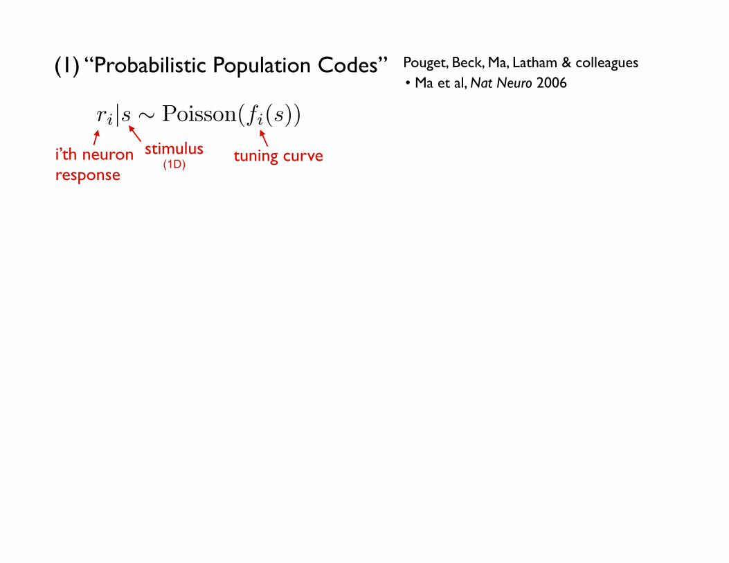
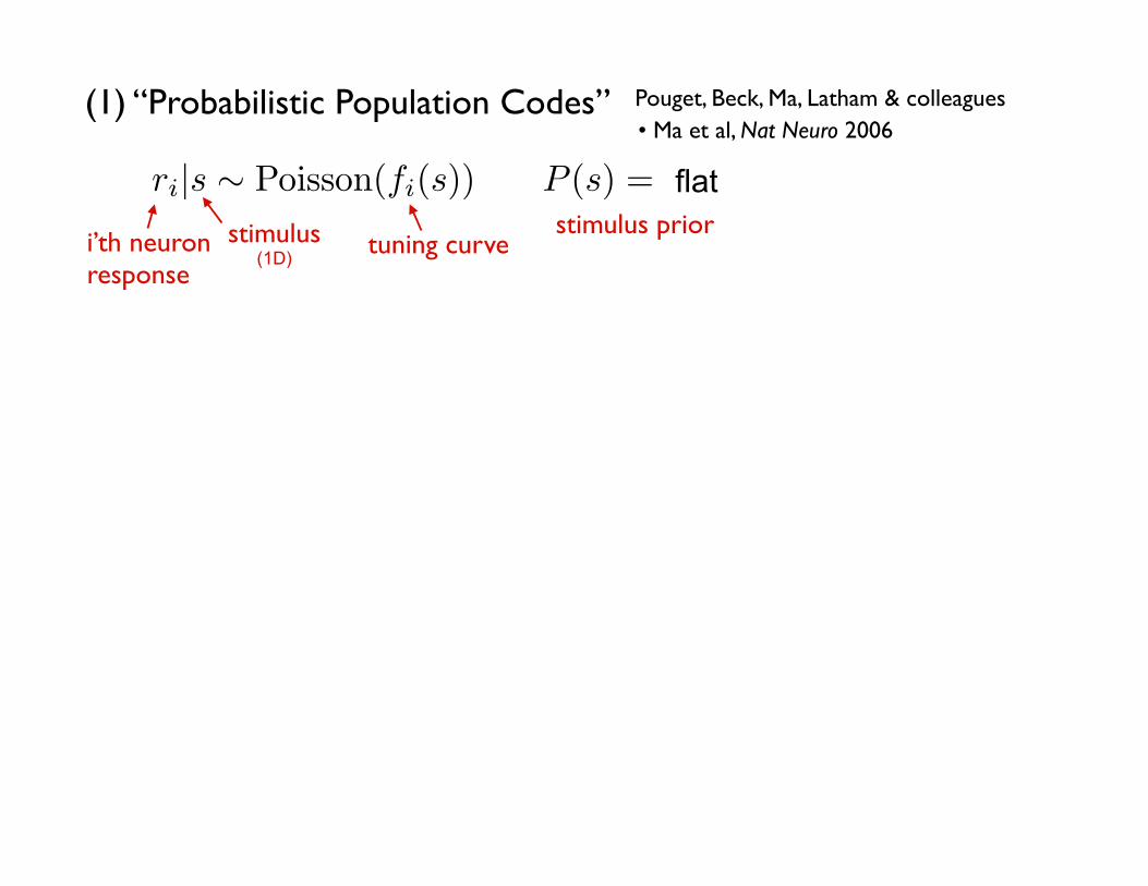
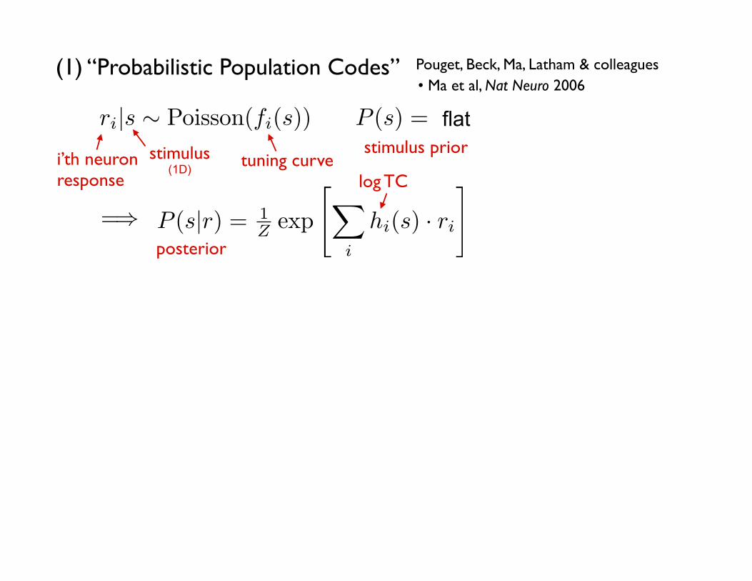
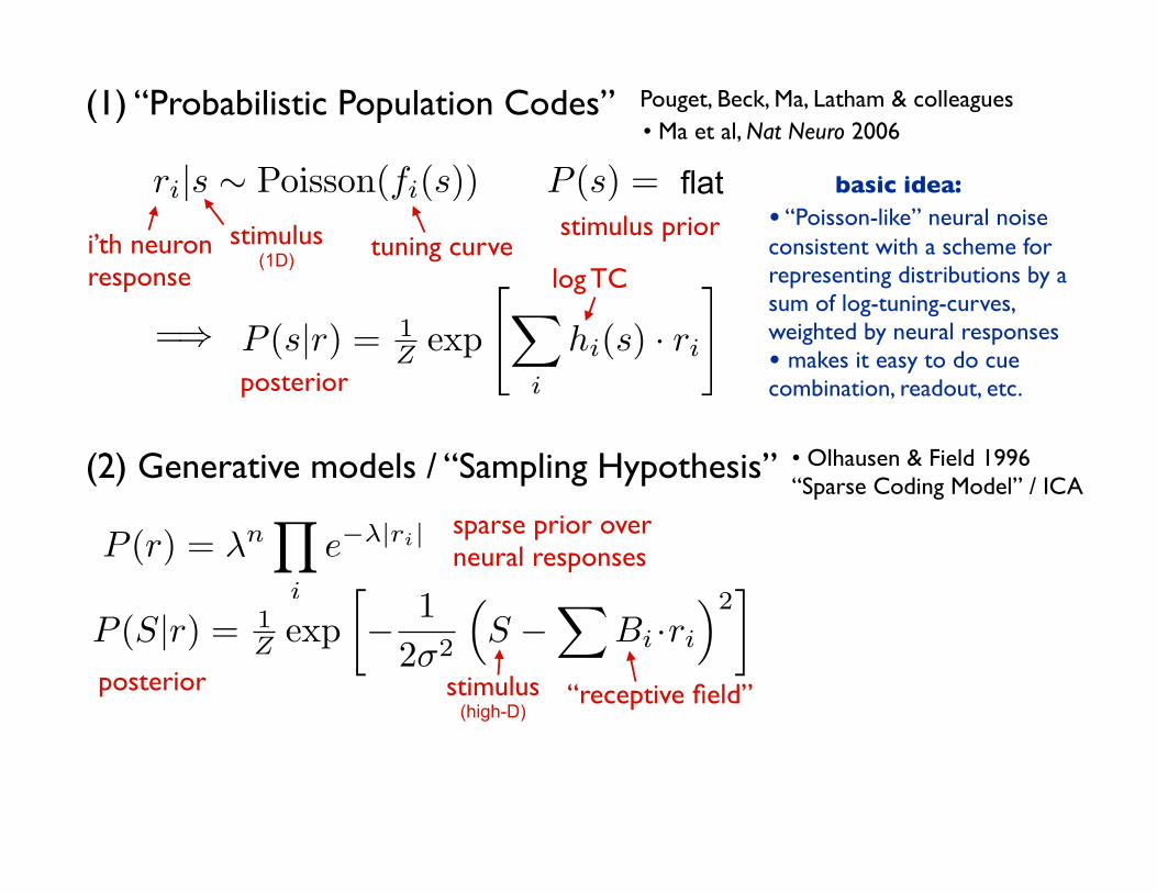
(1) “Probabilistic Population Codes”
tuning curvestimulus(1D)
i’th neuronresponse
Pouget, Beck, Ma, Latham & colleagues• Ma et al, Nat Neuro 2006
(1) “Probabilistic Population Codes”
tuning curvestimulus(1D)
i’th neuronresponse
flatstimulus prior
Pouget, Beck, Ma, Latham & colleagues• Ma et al, Nat Neuro 2006
(1) “Probabilistic Population Codes”
tuning curvestimulus(1D)
i’th neuronresponse
flatstimulus prior
posterior
Pouget, Beck, Ma, Latham & colleagues• Ma et al, Nat Neuro 2006
log TC
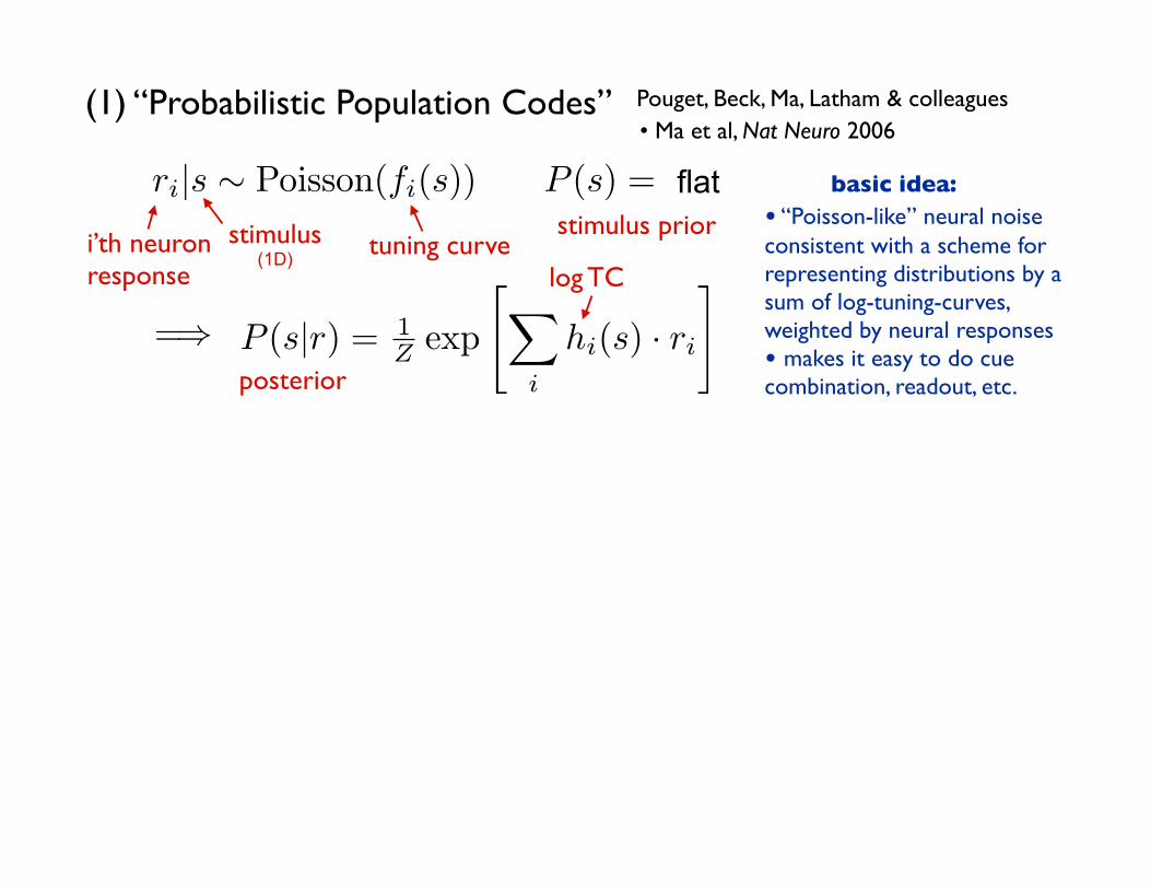
(1) “Probabilistic Population Codes”
tuning curvestimulus(1D)
i’th neuronresponse
flatstimulus prior
posterior
Pouget, Beck, Ma, Latham & colleagues• Ma et al, Nat Neuro 2006
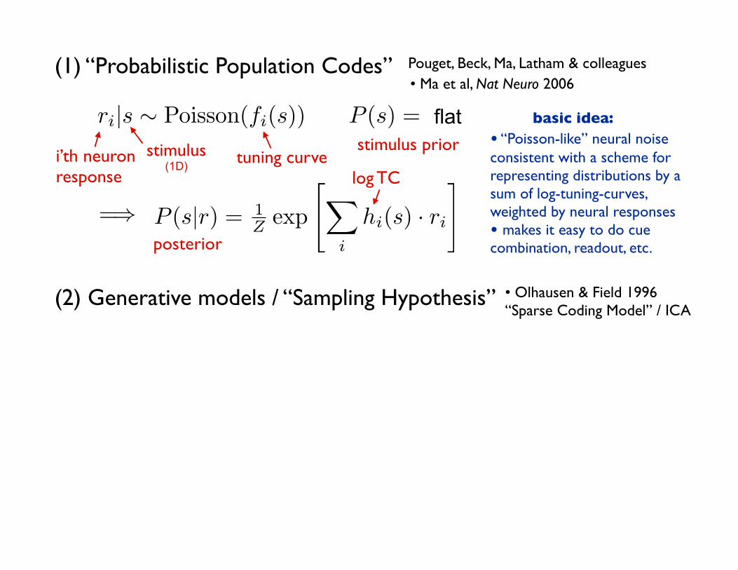
• “Poisson-like” neural noise consistent with a scheme for representing distributions by a sum of log-tuning-curves, weighted by neural responses• makes it easy to do cue combination, readout, etc.
basic idea:
log TC
(1) “Probabilistic Population Codes”
tuning curvestimulus(1D)
i’th neuronresponse
flatstimulus prior
posterior
Pouget, Beck, Ma, Latham & colleagues• Ma et al, Nat Neuro 2006
• “Poisson-like” neural noise consistent with a scheme for representing distributions by a sum of log-tuning-curves, weighted by neural responses• makes it easy to do cue combination, readout, etc.
basic idea:
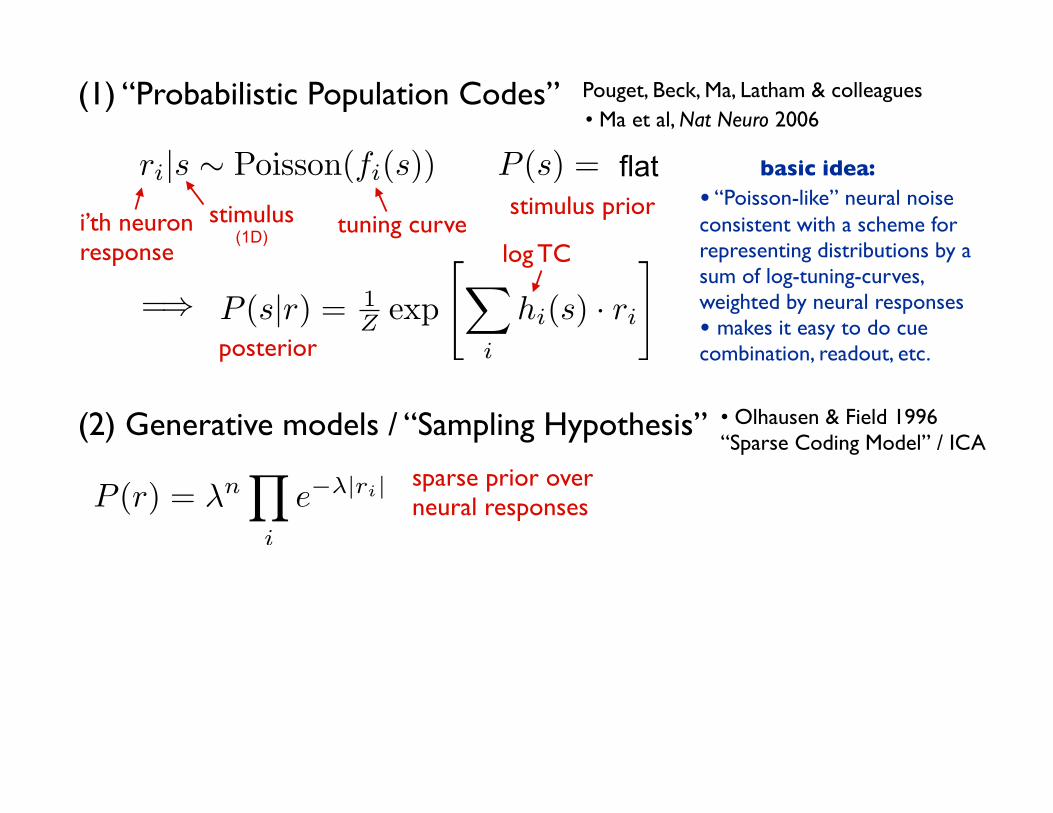
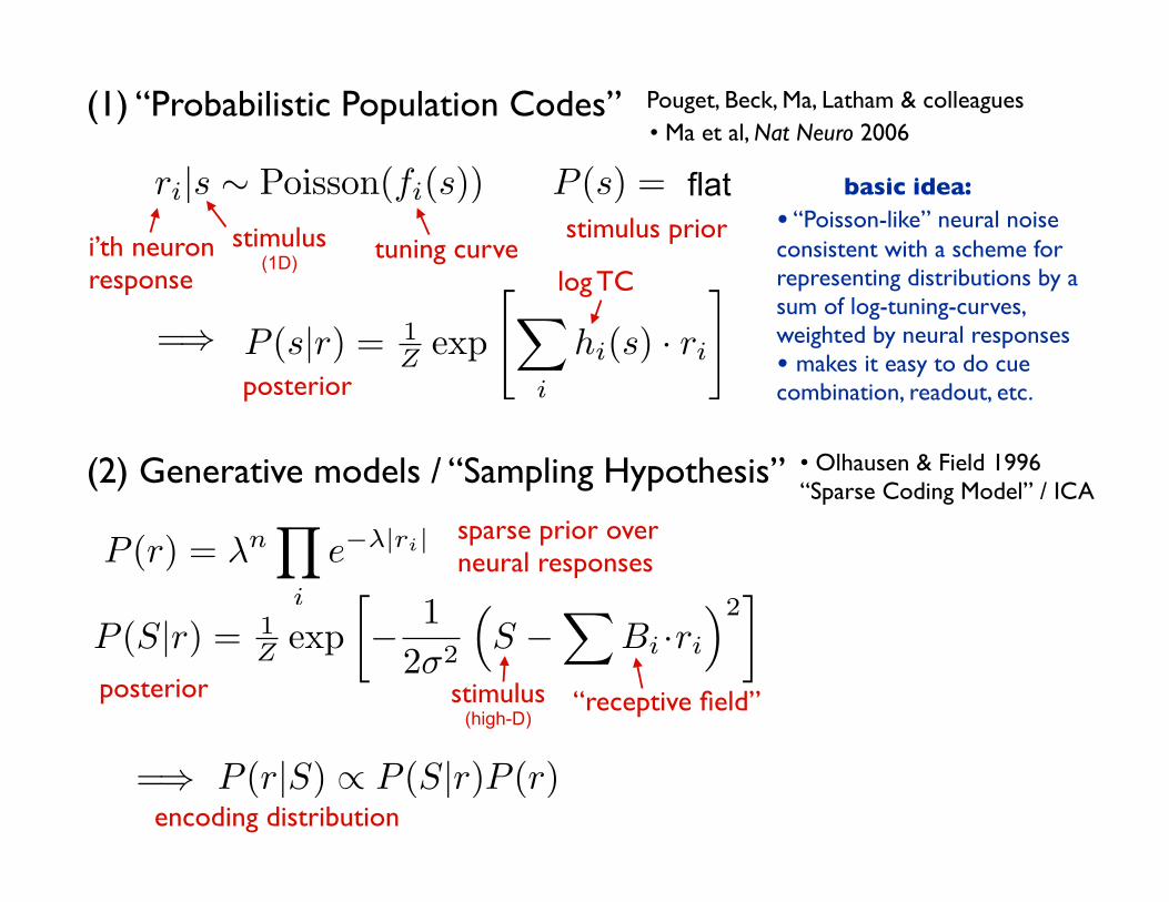
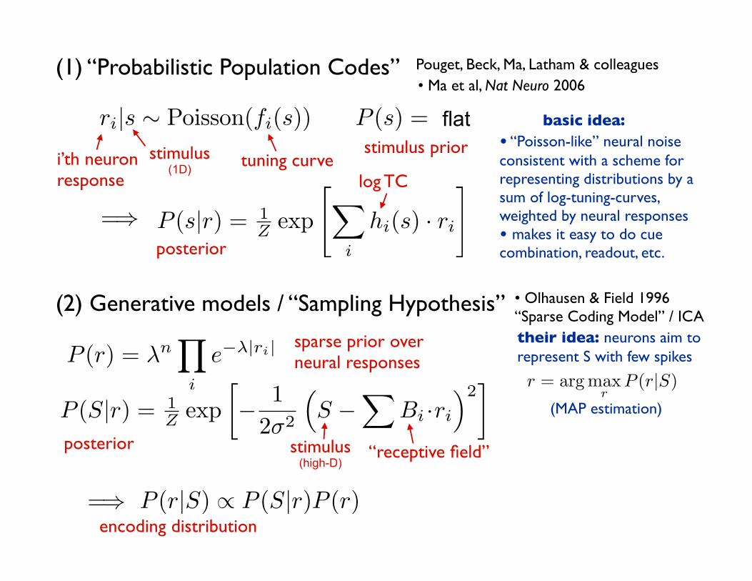
(2) Generative models / “Sampling Hypothesis” • Olhausen & Field 1996“Sparse Coding Model” / ICA
log TC
(1) “Probabilistic Population Codes”
tuning curvestimulus(1D)
i’th neuronresponse
flatstimulus prior
posterior
Pouget, Beck, Ma, Latham & colleagues• Ma et al, Nat Neuro 2006
sparse prior over neural responses
• “Poisson-like” neural noise consistent with a scheme for representing distributions by a sum of log-tuning-curves, weighted by neural responses• makes it easy to do cue combination, readout, etc.
basic idea:
(2) Generative models / “Sampling Hypothesis” • Olhausen & Field 1996“Sparse Coding Model” / ICA
posterior “receptive field”stimulus(high-D)
log TC
(1) “Probabilistic Population Codes”
tuning curvestimulus(1D)
i’th neuronresponse
flatstimulus prior
posterior
Pouget, Beck, Ma, Latham & colleagues• Ma et al, Nat Neuro 2006
sparse prior over neural responses
• “Poisson-like” neural noise consistent with a scheme for representing distributions by a sum of log-tuning-curves, weighted by neural responses• makes it easy to do cue combination, readout, etc.
basic idea:
(2) Generative models / “Sampling Hypothesis” • Olhausen & Field 1996“Sparse Coding Model” / ICA
encoding distribution
posterior “receptive field”stimulus(high-D)
their idea: neurons aim to represent S with few spikes
(MAP estimation)
log TC

(1) “Probabilistic Population Codes”
tuning curvestimulus(1D)
i’th neuronresponse
flatstimulus prior
posterior
Pouget, Beck, Ma, Latham & colleagues• Ma et al, Nat Neuro 2006
sparse prior over neural responses
• “Poisson-like” neural noise consistent with a scheme for representing distributions by a sum of log-tuning-curves, weighted by neural responses• makes it easy to do cue combination, readout, etc.
basic idea:
(2) Generative models / “Sampling Hypothesis” • Olhausen & Field 1996“Sparse Coding Model” / ICA
encoding distribution
posterior “receptive field”stimulus(high-D)
their idea: neurons aim to represent S with few spikes
(MAP estimation)• achieves sparsity• doesn’t represent probability
• Berkes, Orban, Lengyel,Fiser (today):neurons represent P(S|r) with samples
log TC
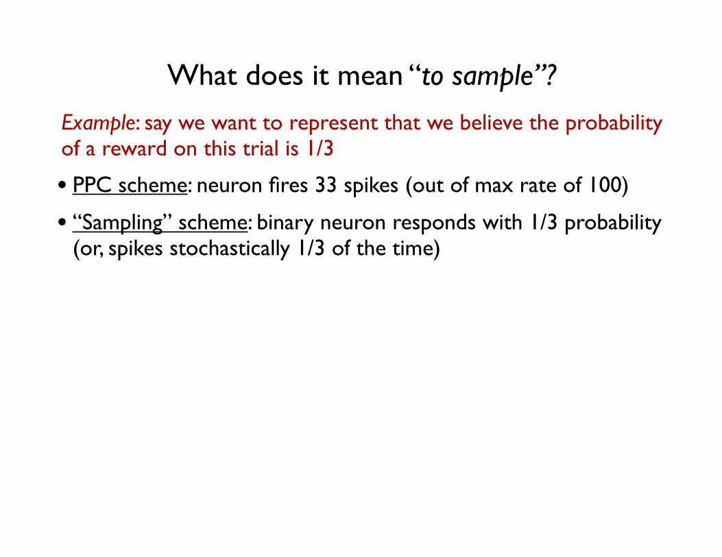
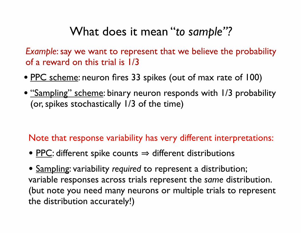
What does it mean “to sample”?
• PPC scheme: neuron fires 33 spikes (out of max rate of 100)
Example: say we want to represent that we believe the probability of a reward on this trial is 1/3
• “Sampling” scheme: binary neuron responds with 1/3 probability (or, spikes stochastically 1/3 of the time)
Note that response variability has very different interpretations:
• PPC: different spike counts ⇒ different distributions
• Sampling: variability required to represent a distribution; variable responses across trials represent the same distribution.(but note you need many neurons or multiple trials to represent the distribution accurately!)

Other differences
• PPC: has nonlinear “tuning curves” (extra layer of abstraction)• Sparse Coding Model (SCM): projective fields are linearly
related to image being represented
• PPC: low-dimensional stimulus (e.g., orientation of a bar)• SCM: high-dimensional stimulus (e.g., image patch)
• PPC: responses are parameters of the distribution represented• Sampling: responses are random variables drawn from a
distribution that is to be represented
Propose different semantics of neural responses:• PPC: a neuron represents “bump” in the posterior distribution• Sampling: neuron represents presence of a given feature in image
Fiser et al, TICS 2010
Stated goal: • why use probabilistic representations• unify “inference” and “learning”
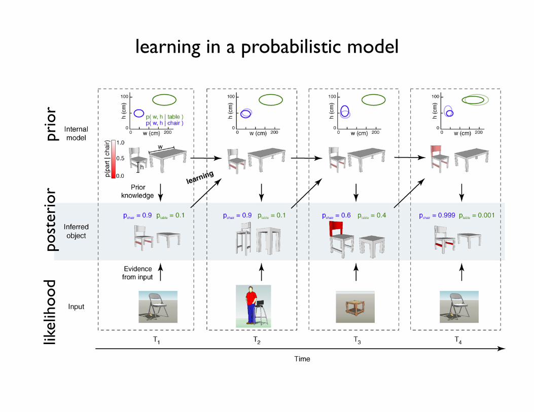
Importantly, just as perception can be formalized as infer-ring hidden states, variables, of the environment from thelimited information provided by sensory input (e.g. infer-ring the true three-dimensional shape and size of the seatof a chair from its two-dimensional projection on ourretinae), learning can be formalized as inferring somemorepersistent hidden characteristics, parameters, of theenvironment based on limited experience. These infer-ences could target concrete physical parameters of objects,such as the typical height or width of a chair, or moreabstract descriptors, such as the possible categories towhich objects can belong (e.g. chairs and tables) (Figure 2).
There are two different ways in which representinguncertainty is important for learning. First, learning aboutour environment modifies the perceptual inferences wedraw from a sensory stimulus. That is, the same stimulusgives rise to different uncertainties after learning. Forexample, having learned about the geometrical propertiesof chairs and tables allows us to increase our confidencethat an unusually looking stool is really more of a chairthan a table (Figure 2). At the neural level, this constrainslearning mechanisms to change neural activity patternssuch that they correctly encode the ensuing changes inperceptual uncertainty, thus keeping the neural repres-entation of uncertainty self-consistent before and afterlearning. Second, representing uncertainty does not justconstrain but also benefits learning. For example, if thereis uncertainty as to whether an object is a chair or a table,our models for both of these categories should be updated,
rather than only updating the model of the most probablecategory (Figure 2). Crucially, the optimal magnitude ofthese updates depends directly (and inversely) on theuncertainty about the object belonging to each category:the model of the more probable category should be updatedto a larger degree [18].
Thus, probabilistic perception implies that learningmust also be probabilistic in nature. Therefore, we nowexamine behavioral and neural evidence for probabilisticlearning.
Probabilistic learning: behavioral levelEvidence for humans and animals being sensitive to theprobabilistic structure of the environment ranges fromlow-level perceptual mechanisms, such as visual groupingmechanisms conforming with the co-occurrence statisticsof line edges in natural scenes [19], to high-level cognitivedecisions such as humans’ remarkably precise predictionsabout the expected life time of processes as diverse as cakebaking or marriages [20]. A recent survey demonstratedhow research in widely different areas ranging from clas-sical forms of animal learning to human learning of sen-sorimotor tasks found evidence of probabilistic learning[21]. It has been found that configural learning in animals[22], causal learning in rats [23] as well as in humaninfants [24] and a vast array of inductive learning phenom-ena fit comfortably with a hierarchical probabilistic frame-work, in which probabilistic learning is performed atincreasingly higher levels of abstraction [25].
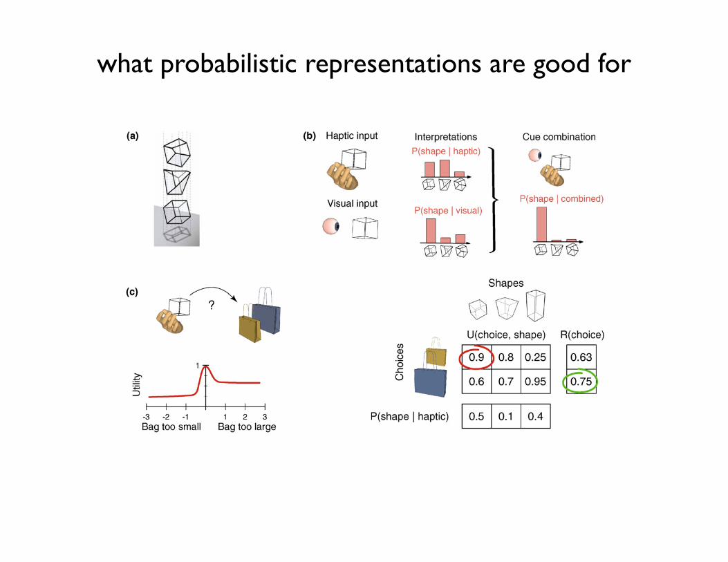
Figure 1. Representation of uncertainty and its benefits. (a) Sensory information is inherently ambiguous. Given a two-dimensional projection on a surface (e.g. a retina), itis impossible to determine which of the three different three-dimensional wire frame objects above cast the image (adapted with permission from [96]). (b) Cue integration.Independent visual and haptic measurements (left) support to different degrees the three possible interpretations of object identity (middle). Integrating these sources ofinformation according to their respective uncertainties provides an optimal probabilistic estimate of the correct object (right). (c) Decision-making. When the task is tochoose the bag with the right size for storing an object, uncertain haptic information needs to be utilized probabilistically for optimal choice (top left). In the example shown,the utility function expresses the degree to which a combination of object and bag size is preferable: for example, if the bag is too small, the object will not fit in, if it is toolarge, we are wasting valuable bag space (bottom left, top right). In this case, rather than inferring the most probable object based on haptic cues and then choosing the bagoptimal for that object (in the example, the small bag for the cube), the probability of each possible object needs to be weighted by its utility and the combination with thehighest expected utility (R) has to be selected (in the example, the large bag has the highest expected utility). Evidence shows that human performance in cue combinationand decision-making tasks is close to optimal [10,97].
Review Trends in Cognitive Sciences Vol.14 No.3
121
what probabilistic representations are good for
Aparticularly direct line of evidence for humans learningcomplex, high-dimensional distributions of many variablesby performing higher-order probabilistic learning, not justnaı̈ve frequency-based learning, comes from the domain ofvisual statistical learning (Box 1). An analysis of a series ofvisual statistical learning experiments showed that beyondthe simplest results, recursive pairwise associative learningis inadequate for replicating human performance, whereasBayesian probabilistic learning not only accurately repli-cates these results but it makes correct predictions abouthuman performance in new experiments [26].
These examples suggest a common core representationaland learning strategy for animals and humans that showsremarkable statistical efficiency. However, such behavioralstudies provide no insights as to how these strategies mightbe implemented in the neural circuitry of the cortex.
Probabilistic learning in the cortex: neural levelAlthough psychophysical evidence has been steadily grow-ing, there is little direct electrophysiological evidenceshowing that learning and development in neural systemsis optimal in a statistical sense even though the effect of
learning on cortical representations has been investigatedextensively [27,28]. One of the main reasons for this is thatthere have been very few plausible computational modelsproposed for a neural implementation of probabilisticlearning that would provide easily testable predictions(but see Refs [29,30]). Here, we give a brief overview ofthe computational approaches developed to capture prob-abilistic learning in neural systems and discuss why theyare unsuitable in their current form for being tested inelectrophysiological experiments.
Classical work on connectionist models aimed at devis-ing neural networks with simplified neural-like units thatcould learn about the regularities hidden in a stimulusensemble [31]. This line of research has been developedfurther substantially and demonstrated explicitly howdynamical interactions between neurons in these networkscorrespond to computing probabilistic inferences, and howthe tuning of synaptic weights corresponds to learning theparameters of a probabilistic model of input stimuli [32–34]. A key common feature in these statistical neural net-works is that inference and learning are inseparable:inference relies on the synaptic weights encoding a useful
Figure 2. The link between probabilistic inference and learning. (Top row) Developing internal models of chairs and tables. The plot shows the distribution of parameters (two-dimensional Gaussians, represented by ellipses) and object shapes for the two categories. (Middle row) Inferences about the currently viewed object based on the input and theinternal model. (Bottom row) Actual sensory input. Red color code represents the probability of a particular object part being present (see color scale on top left). T1–T4, foursuccessive illustrative iterations of the inference–learning cycle. (T1) The interpretation of a natural scene requires combining information from the sensory input (bottom) andthe internal model (top). Based on the internal models of chairs and tables, the input is interpreted with high probability (p = 0.9) as a chair with a typical size but missingcrossbars (middle). (T2) The internalmodel of theworld is updated based on the cumulative experience of previous inferences (top). The chair in T1, being a typical example of achair, requiresminimal adjustments to the internalmodel. Experience withmore unusual instances, as for example the high chair in T2, provokesmore substantial changes (T3,top). (T3) The representation of uncertainty allows to update the internalmodel taking into account all possible interpretations of the input. In T3, the stimulus is ambiguous as itcould be interpreted as a stool, or a square table. The internalmodel needs to be updated by taking into account the relative probability of the two interpretations: that there existtables with a more square shape or that some chairs miss the upper part. Since both probabilities are relatively high, both internal models will bemodified substantially duringlearning (see the change of both ellipses). (T4) After learning, the same input as in T1 elicits different responses owing to changes in the internal model. In T4, the input isinterpreted as a chair with significantly higher confidence, as experience has shown that chairs often lack the bottom crossbars.
Review Trends in Cognitive Sciences Vol.14 No.3
122
learning in a probabilistic modelpr
ior
likel
ihoo
dpo
ster
ior
statistical learning in humans
probabilistic model of the environment, whereas learningproceeds by using the inferences produced by the network(Figure 3a).
Although statistical neural networks have considerablygrown in sophistication and algorithmic efficiency in recentyears [35], providing cutting-edge performance in somechallenging real-world machine learning tasks, much less
attention has been devoted to specifying their biologicalsubstrates. At the level of general insights, these modelssuggestedways in which internally generated spontaneousactivity patterns (‘‘fantasies’’) that are representative ofthe probabilistic model encoded by the neural network canhave important roles in the fine tuning of synapses duringoff-line periods of functioning. They also clarified that
Box 1. Visual statistical learning in humans
In experimental psychology, the term ‘‘statistical learning’’ refers to aparticular type of implicit learning that emerged from investigatingartificial grammar learning. It is fundamentally different from traditionalperceptual learning andwas first used in the domain of infant languageacquisition [72]. The paradigm has been adapted from auditory to othersensory modalities such as touch and vision, to different species andvarious aspects of statistical learning have been explored such asmultimodal interactions [73], effects of attention, interaction withabstract rule learning [74], together with its neural substrates [75].The emerging consensus based on these studies is that statisticallearning is a domain-general, fundamental learning ability of humansand animals that is probably a major component of the process bywhich internal representations of the environment are developed.
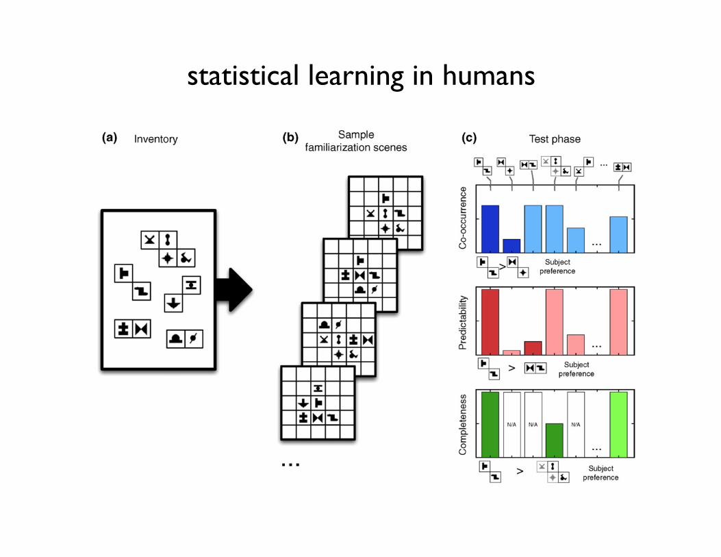
The basic idea of the statistical learning paradigm is to create anartificial mini-world by using a set of building blocks to generateseveral composite inputs that represent possible instances in thisworld. In the case of visual statistical learning (VSL), artificial visualscenes are composed from abstract shape elements where thebuilding blocks are two or more such shapes always appearing inthe same relative configuration (Figure I). An implicit learningparadigm is used to test how internal visual representations emergethrough passively observing a large number of such composite
scenes without any instruction as to what to pay attention to. Afterbeing exposed to the scenes, when subjects have to choose betweentwo fragments of shape combinations based on familiarity, theyreliably more often choose fragments that were true building blocksof the scenes compared to random combinations of shapes [76].Similar results were found in 8-month-old infants [77,78] suggestingthat humans from an early age can automatically extract theunderlying structure of an unknown sensory data set based purelyon statistical characteristics of the input.Investigations of VSL provided evidence of increasingly sophisti-
cated aspects of this learning, setting it apart from simple frequency-based naı̈ve learning methods. Subjects not only automaticallybecome sensitive to pairs of shapes that appear more frequentlytogether, but also to pairs with elements that are more predictive ofeach other even when the co-occurrence of those elements is notparticularly high [76]. Moreover, this learning highly depends onwhether or not a pair of elements is a part of a larger buildingstructure, such as a quadruple [79]. Thus, it appears that humanstatistical learning is a sophisticated mechanism that is not onlysuperior to pairwise associative learning but also potentially capableto link appearance-based simple learning and higher-level ‘‘rule-learning’’ [26].
Figure I. Visual statistical learning. (a) An inventory of visual chunks is defined as a set of two or more spatially adjacent shapes always co-occurring in scenes. (b) Sampleartificial scenes composed ofmultiple chunks that are used in the familiarization phase. Note that there are noobvious low-level segmentation cues giving away the identity ofthe underlying chunks. (c) During the test phase, subjects are shown pairs of segments that are either parts of chunks or random combinations (segments on the top). Thethree histograms show different statistical conditions. (Top) There is a difference in co-occurrence frequency of elements between the two choices; (middle) co-occurrence isequated, but there is difference in predictability (the probability of one symbol given that the other is present) between the choices; (bottom) both co-occurrence andpredictability are equated between the two choices, but the completeness statistics (what percentage of a chunk in the inventory is covered by the choice fragment) is different– one pair is a standalone chunk, the other is a part of a larger chunk. Subjects were able to use cues in any of these conditions, as indicated by the subject preferences beloweach panel. These observations can be accounted for by optimal probabilistic learning, but not by simpler alternatives such as pairwise associative learning (see text).
Review Trends in Cognitive Sciences Vol.14 No.3
123
probabilistic inference and learning with neurons
useful learning rules for such tuning always include Heb-bian as well as anti-Hebbian terms [32,33]. In addition,several insightful ideas about the roles of bottom-up,recurrent, and top-down connections for efficient inferenceand learning have also been put forward [36–38], but theywere not specified at a level that would allow direct exper-imental tests.
Learning internal models of natural images hastraditionally been one area where the biological relevanceof statistical neural networks was investigated. As thesestudies aimed at explaining the properties of early sensoryareas, the ‘‘objects’’ they learned to infer were simplelocalized and oriented filters assumed to interact mostlyadditively in creating images (Figure 3b). Although theserepresentations are at a lower level than the ‘‘true’’ objectsconstituting our environment (such as chairs and tables)that typically interact in highly non-linear ways as theyform images (owing to e.g. occlusion [39]), the same prin-ciples of probabilistic inference and learning also apply tothis level. Indeed, several studies showed how probabilisticlearning of natural scene statistics leads to representa-tions that are similar to those found in simple and complexcells of the visual cortex [40–44]. Although some earlystudies were not formulated originally in a statisticalframework [40,41,43], later theoretical developmentsshowed that their learning algorithms were in fact specialcases of probabilistic learning [45,46].
The general method of validation in these learningstudies almost exclusively concentrated on comparingthe ‘‘receptive field’’ properties of model units with thoseof sensory cortical neurons and showing a good matchbetween the two. However, as the emphasis in many ofthese models is on learning, the details of the mapping of
neural dynamics to inference were left implicit (with somenotable exceptions [44,47]). In cases where inference hasbeen defined explicitly, neurons were usually assumed torepresent single deterministic (so-called ‘‘maximum a pos-teriori’’) estimates (Figure 3b). This failure to representuncertainty is not only computationally harmful for infer-ence, decision-making and learning (Figures 1–2) but it isalso at odds with behavioral data showing that humansand animals are influenced by perceptual uncertainty.Moreover, this approach constrains predictions to be madeonly about receptive fields which often says little abouttrial-by-trial, on-line neural responses [48].
In summary, presently a main challenge in probabilisticneural computation is to pinpoint representationalschemes that enable neural networks to represent uncer-tainty in a physiologically testable manner. Specifically,learning with such representations on naturalistic inputshould provide verifiable predictions about the corticalimplementation of these schemes beyond receptive fields.
Probabilistic representations in the cortex for inferenceand learningThe conclusion of this review so far is that identifying theneural representation of uncertainty is key for understand-ing how the brain implements probabilistic inference andlearning. Crucially, because inference and learning areinseparable, a viable candidate representational schemeshould be suitable for both. In line with this, evidence isgrowing that perception and memory-based familiarityprocesses once thought to be linked to anatomically clearlysegregated cortical modules along the ventral pathway ofthe visual cortex could rely on integrated multipurposerepresentations within all areas [49]. In this section, we
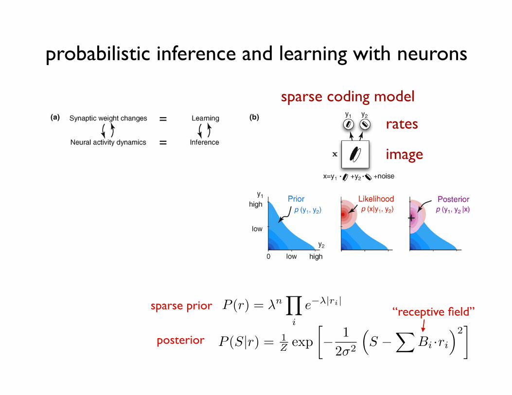
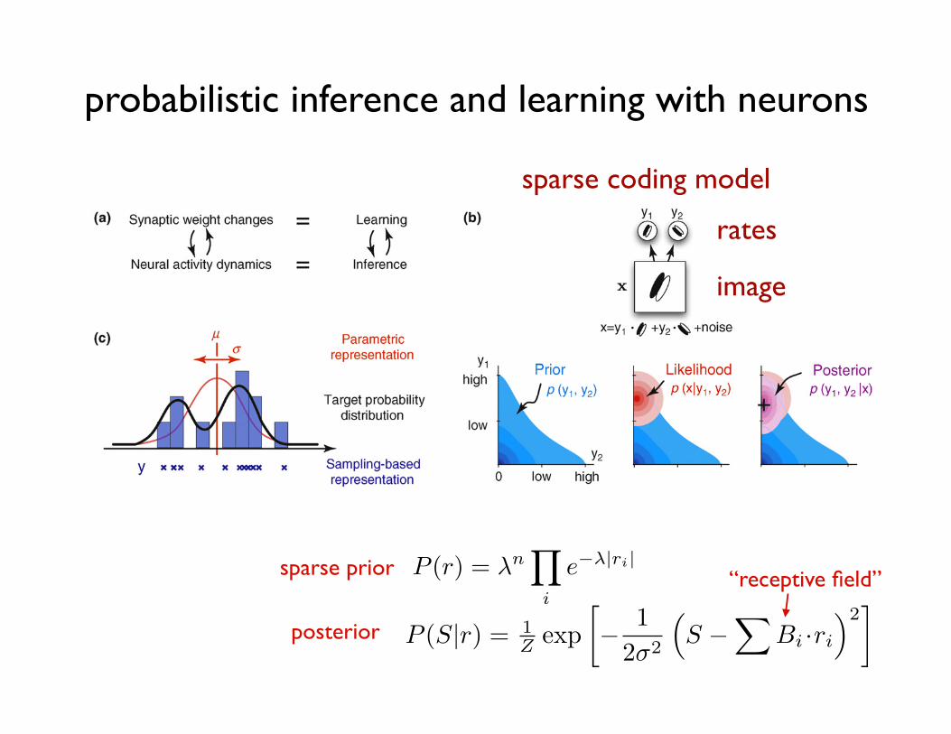
Figure 3. Neural substrates of probabilistic inference and learning. (a) Functional mapping of learning and inference onto neural substrates in the cortex. (b) Probabilisticinference for natural images. (Top) A toy model of the early visual system (based on Ref. [43]). The internal model of the environment assumes that visual stimuli, x, aregenerated by the noisy linear superposition of two oriented features with activation levels, y1 and y2. The task of the visual system is to infer the activation levels, y1 and y2,of these features from seeing only their superposition, x. (Bottom left) The prior distribution over the activation of these features, y1 and y2, captures prior knowledge abouthow much they are typically (co-)activated in images experienced before. In this example, y1 and y2 are expected to be independent and sparse, which means that eachfeature appears rarely in visual scenes and independently of the other feature. (Bottom middle) The likelihood function represents the way the visual features are assumedto combine to form the visual input under our model of the environment. It is higher for feature combinations that are more likely to underlie the image we are seeingaccording to the equation on the top. (Bottom right) The goal of the visual system is to infer the posterior distribution over y1 and y2. By Bayes’ theorem, the posterioroptimally combines the expectations from the prior with the evidence from the likelihood. Maximum a posteriori (MAP) estimate, used by some models [40,43,47], denotedby a + in the figure neglects uncertainty by using only the maximum value instead of the full distribution. (c) Simple demonstration of two probabilistic representationalschemes. (Black curve) The probability distribution of variable y to be represented. (Red curve) Assumed distribution by the parametric representation. Only the twoparameters of the distribution, the mean m and variance s are represented. (Blue ‘‘x’’-s and bars) Samples and the histogram implied by the sampling-based representation.
Review Trends in Cognitive Sciences Vol.14 No.3
124
sparse coding model
rates
image
sparse prior
posterior
“receptive field”
probabilistic inference and learning with neurons
useful learning rules for such tuning always include Heb-bian as well as anti-Hebbian terms [32,33]. In addition,several insightful ideas about the roles of bottom-up,recurrent, and top-down connections for efficient inferenceand learning have also been put forward [36–38], but theywere not specified at a level that would allow direct exper-imental tests.
Learning internal models of natural images hastraditionally been one area where the biological relevanceof statistical neural networks was investigated. As thesestudies aimed at explaining the properties of early sensoryareas, the ‘‘objects’’ they learned to infer were simplelocalized and oriented filters assumed to interact mostlyadditively in creating images (Figure 3b). Although theserepresentations are at a lower level than the ‘‘true’’ objectsconstituting our environment (such as chairs and tables)that typically interact in highly non-linear ways as theyform images (owing to e.g. occlusion [39]), the same prin-ciples of probabilistic inference and learning also apply tothis level. Indeed, several studies showed how probabilisticlearning of natural scene statistics leads to representa-tions that are similar to those found in simple and complexcells of the visual cortex [40–44]. Although some earlystudies were not formulated originally in a statisticalframework [40,41,43], later theoretical developmentsshowed that their learning algorithms were in fact specialcases of probabilistic learning [45,46].
The general method of validation in these learningstudies almost exclusively concentrated on comparingthe ‘‘receptive field’’ properties of model units with thoseof sensory cortical neurons and showing a good matchbetween the two. However, as the emphasis in many ofthese models is on learning, the details of the mapping of
neural dynamics to inference were left implicit (with somenotable exceptions [44,47]). In cases where inference hasbeen defined explicitly, neurons were usually assumed torepresent single deterministic (so-called ‘‘maximum a pos-teriori’’) estimates (Figure 3b). This failure to representuncertainty is not only computationally harmful for infer-ence, decision-making and learning (Figures 1–2) but it isalso at odds with behavioral data showing that humansand animals are influenced by perceptual uncertainty.Moreover, this approach constrains predictions to be madeonly about receptive fields which often says little abouttrial-by-trial, on-line neural responses [48].
In summary, presently a main challenge in probabilisticneural computation is to pinpoint representationalschemes that enable neural networks to represent uncer-tainty in a physiologically testable manner. Specifically,learning with such representations on naturalistic inputshould provide verifiable predictions about the corticalimplementation of these schemes beyond receptive fields.
Probabilistic representations in the cortex for inferenceand learningThe conclusion of this review so far is that identifying theneural representation of uncertainty is key for understand-ing how the brain implements probabilistic inference andlearning. Crucially, because inference and learning areinseparable, a viable candidate representational schemeshould be suitable for both. In line with this, evidence isgrowing that perception and memory-based familiarityprocesses once thought to be linked to anatomically clearlysegregated cortical modules along the ventral pathway ofthe visual cortex could rely on integrated multipurposerepresentations within all areas [49]. In this section, we
Figure 3. Neural substrates of probabilistic inference and learning. (a) Functional mapping of learning and inference onto neural substrates in the cortex. (b) Probabilisticinference for natural images. (Top) A toy model of the early visual system (based on Ref. [43]). The internal model of the environment assumes that visual stimuli, x, aregenerated by the noisy linear superposition of two oriented features with activation levels, y1 and y2. The task of the visual system is to infer the activation levels, y1 and y2,of these features from seeing only their superposition, x. (Bottom left) The prior distribution over the activation of these features, y1 and y2, captures prior knowledge abouthow much they are typically (co-)activated in images experienced before. In this example, y1 and y2 are expected to be independent and sparse, which means that eachfeature appears rarely in visual scenes and independently of the other feature. (Bottom middle) The likelihood function represents the way the visual features are assumedto combine to form the visual input under our model of the environment. It is higher for feature combinations that are more likely to underlie the image we are seeingaccording to the equation on the top. (Bottom right) The goal of the visual system is to infer the posterior distribution over y1 and y2. By Bayes’ theorem, the posterioroptimally combines the expectations from the prior with the evidence from the likelihood. Maximum a posteriori (MAP) estimate, used by some models [40,43,47], denotedby a + in the figure neglects uncertainty by using only the maximum value instead of the full distribution. (c) Simple demonstration of two probabilistic representationalschemes. (Black curve) The probability distribution of variable y to be represented. (Red curve) Assumed distribution by the parametric representation. Only the twoparameters of the distribution, the mean m and variance s are represented. (Blue ‘‘x’’-s and bars) Samples and the histogram implied by the sampling-based representation.
Review Trends in Cognitive Sciences Vol.14 No.3
124
sparse coding model
rates
image
sparse prior
posterior
“receptive field”
How to represent a 2D distribution
Box 2. Probabilistic representational schemes for inference and learning
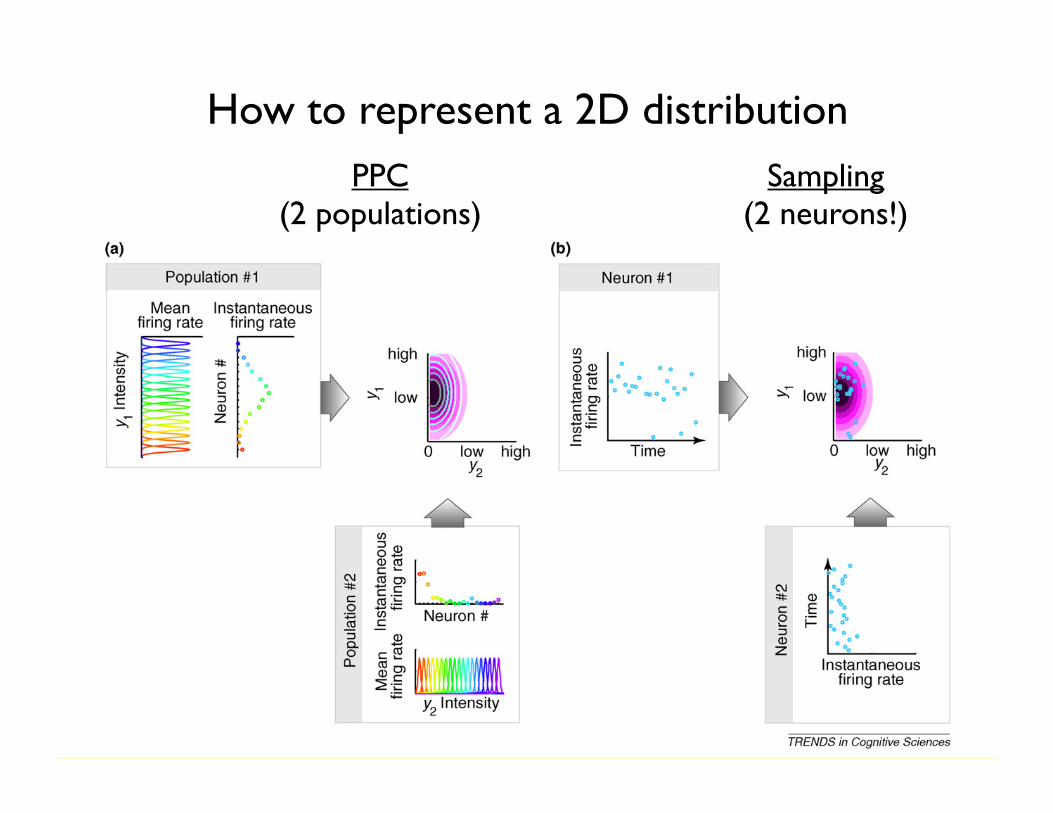
Representing uncertainty associated with sensory stimuli requiresneurons to represent the probability distribution of the environmentalvariables that are being inferred. One class of schemes calledprobabilistic population codes (PPCs) assumes that neurons corre-spond to parameters of this distribution (Figure Ia). A simple buthighly unfeasible version of this scheme would be if different neuronsencoded the elements of the mean vector and covariance matrix of amultivariate Gaussian distribution. At any given time, the activities ofneurons in PPCs provide a complete description of the distribution bydetermining its parameters, making PPCs and other parametricrepresentational schemes particularly suitable for real-time inference[80–82]. Given that, in general, the number of parameters required tospecify a multivariate distribution scales exponentially with thenumber of its variables, a drawback of such schemes is that thenumber of neurons needed in an exact PPC representation would beexponentially large and with fewer neurons the representationbecomes approximate. Characteristics of the family of representableprobability distributions by this scheme are determined by thecharacteristics of neural tuning curves and noisiness [16] (Table I).
An alternative scheme to represent probability distributions inneural activities is based on each neuron corresponding to one of theinferred variables. For example, each neuron can encode the value ofone of the variables of a multivariate Gaussian distribution. Inparticular, the activity of a neuron at any time can represent a samplefrom the distribution of that variable and a ‘‘snapshot’’ of the activitiesof many neurons therefore can represent a sample from a high-dimensional distribution (Figure Ib). Such a representation requirestime to take multiple samples (i.e. a sequence of firing ratemeasurements) for building up an increasingly reliable estimate ofthe represented distribution which might be prohibitive for on-lineinference, but it does not require exponentially many neurons and —given enough time — it can represent any distribution (Table I). Afurther advantage of collecting samples is that marginalization, animportant case of computing integrals that infamously plaguepractical Bayesian inference, learning and decision-making, becomesa straightforward neural operation. Finally, although it is unclear howprobabilistic learning can be implemented with PPCs, sampling basedrepresentations seem particularly suitable for it (see main text).
Figure I. Two approaches to neural representations of uncertainty in the cortex. (a) Probabilistic population codes rely on a population of neurons that are tuned to thesame environmental variables with different tuning curves (populations 1 and 2, colored curves). At any moment in time, the instantaneous firing rates of these neurons(populations 1 and 2, colored circles) determine a probability distribution over the represented variables (top right panel, contour lines), which is an approximation ofthe true distribution that needs to be represented (purple colormap). In this example, y1 and y2, are independent, but in principle, there could be a single population withneurons tuned to both y1 and y2. However, such multivariate representations require exponentially more neurons (see text and Table I). (b) In a sampling basedrepresentation, single neurons, rather than populations of neurons, correspond to each variable. Variability of the activity of neurons 1 and 2 through time representsuncertainty in environmental variables. Correlations between the variables can be naturally represented by co-variability of neural activities, thus allowing therepresentation of arbitrarily shaped distributions.
Table I. Comparing characteristics of the two main modeling approaches to probabilistic neural representationsPPCs Sampling-based
Neurons correspond to Parameters VariablesNetwork dynamics required (beyond the first layer) Deterministic Stochastic (self-consistent)Representable distributions Must correspond to a particular
parametric formCan be arbitrary
Critical factor in accuracy of encoding a distribution Number of neurons Time allowed for samplingInstantaneous representation of uncertainty Complete, the whole distribution is
represented at any timePartial, a sequence of samplesis required
Number of neurons needed for representingmultimodal distributions
Scales exponentially with thenumber of dimensions
Scales linearly with the number ofdimensions
Implementation of learning Unknown Well-suited
Review Trends in Cognitive Sciences Vol.14 No.3
126
PPC(2 populations)
Sampling(2 neurons!)
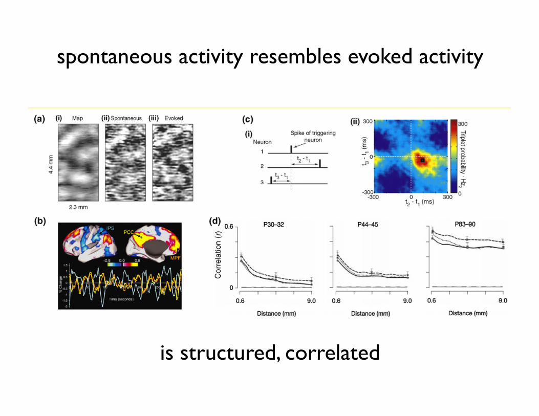
spontaneous activity resembles evoked activity
The posterior distribution is inferred by combining infor-mation from two sources: the sensory input, and the priordistribution describing a priori beliefs about the sensoryenvironment (Figure 3b). Intuitively, in the absence ofsensory stimulation, this distribution will collapse to theprior distribution, and spontaneous activity will representthis prior (Figure 4).
This proposal linking spontaneous activity to the priordistribution has implications that can address many of theissues developed in this review. It provides an account ofspontaneous activity that is consistent with one of its mainfeatures: its remarkable similarity to evoked activity[64,66,67]. A general feature of statistical models thatare appropriately describing their inputs is that the priordistribution and the average posterior distribution closelymatch each other [68]. Thus, if evoked and spontaneous
activities represent samples from the posterior and priordistributions, respectively, under an appropriate model ofthe environment, they are expected to be similar [53]. Inaddition, spontaneous activity itself, as prior expectation,should be sufficient to evoke firing in some cells withoutsensory input, as was observed experimentally [67].
Statistical neural networks also suggest that samplingfrom the prior can be more than just a byproduct ofprobabilistic inference: it can be computationally advan-tageous for the functioning of the network. In the absenceof stimulation, during awake spontaneous activity,sampling from the prior can help with driving the networkclose to states that are probable to be valid inferences onceinput arrives, thus potentially shortening the reaction timeof the system [69]. This ‘‘priming’’ effect could present analternative account of why human subjects are able to sort
Box 3. Spontaneous activity in the cortex
Spontaneous activity in the cortex is defined as ongoing neural activityin the absence of sensory stimulation [83]. This definition is the clearestin the case of primary sensory cortices where neural activity hastraditionally been linked very closely to sensory input. Despite someearly observations that it can influence behavior, cortical spontaneousactivity has been considered stochastic noise [84]. The discovery ofretinal and later cortical waves [85] of neural activity in the maturingnervous system has changed this view in developmental neuroscience,igniting an ongoing debate about the possible functional role of suchspontaneous activity during development [86].
Several recent results based on the activities of neural populationsinitiated a similar shift in view about the role of spontaneous activityin the cortex during real-time perceptual processes [65]. Imaging andmulti-electrode studies showed that spontaneous activity has largescale spatiotemporal structure over millimeters of the cortical surface,that the mean amplitude of this activity is comparable to that ofevoked activity and it links distant cortical areas together [64,87,88](Figure I). Given the high energy cost of cortical spike activity [89],these findings argue against the idea of spontaneous activity beingmere noise. Further investigations found that spontaneous activityshows repetitive patterns [90,91], it reflects the structure of the
underlying neural circuitry [67], which might represent visualattributes [66], that the second order correlational structure ofspontaneous and evoked activity is very similar and it changessystematically with age [64]. Thus, cell responses even in primarysensory cortices are determined by the combination of spontaneousand bottom-up, external stimulus-driven activity.The link between spontaneous and evoked activity is further
promoted by findings that after repetitive presentation of a sensorystimulus, spontaneous activity exhibits patterns of activity reminis-cent to those seen during evoked activity [92]. This suggests thatspontaneous activity might be altered on various time scales leadingto perceptual adaptation and learning. These results led to anincreasing consensus that spontaneous activity might have a func-tional role in perceptual processes that is related to internal states ofcell assemblies in the brain, expressed via top-down effects thatembody expectations, predictions and attentional processes [93] andmanifested in modulating functional connectivity of the network [94].Although there have been theoretical proposals of how bottom-upand top-down signals could jointly define perceptual processes[55,95], the rigorous functional integration of spontaneous activityin such a framework has emerged only recently [53].
Figure I. Characteristics of cortical spontaneous activity. (a) There is a significant correlation between the orientation map of the primary visual cortex of anesthetizedcat (left panel), optical image patterns of spontaneous (middle panel) and visually evoked activities (right panel) (adapted with permission from [66]). (b) Correlationalanalysis of BOLD signals during resting state reveals networks of distant areas in the human cortex with coherent spontaneous fluctuations. There are large scalepositive intrinsic correlations between the seed region PCC (yellow) and MPF (orange) and negative correlations between PCC and IPS (blue) (adapted with permissionfrom [98]). (c) Reliably repeating spike triplets can be detected in the spontaneous firing of the rat somatosensory cortex by multielectrode recording (adapted withpermission from [91]). (d) Spatial correlations in the developing awake ferret visual cortex of multielectrode recordings show a systematic pattern of emerging strongcorrelations across several millimeters of the cortical surface and very similar correlational patterns for dark spontaneous (solid line) and visually driven conditions(dotted and dashed lines for random noise patterns and natural movies, respectively) (adapted with permission from [64]).
Review Trends in Cognitive Sciences Vol.14 No.3
127
is structured, correlated
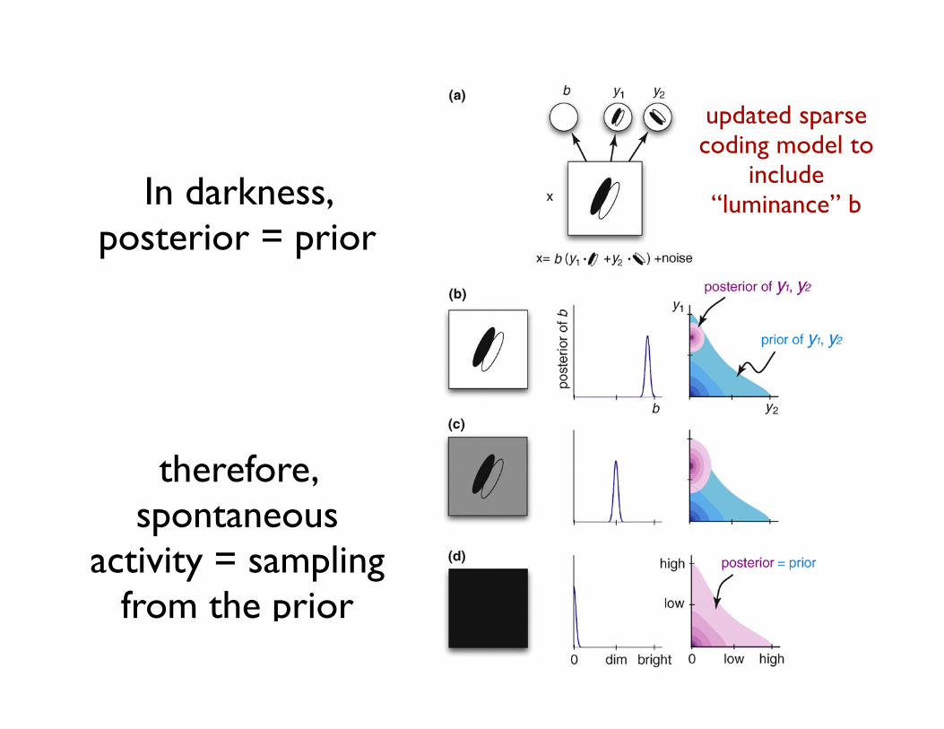
In darkness, posterior = prior
images into natural/non-natural categories in a matter of!150 ms [70], which is traditionally taken as evidence forthe dominance of feed-forward processing in the visualsystem [71]. Finally, during off-line periods, such as sleep-ing, sampling from the prior could have a role in tuningsynaptic weights thus contributing to the refinement of theinternal model of the sensory environment as suggested bystatistical neural network models [32,33].
Importantly, the proposal that spontaneous activityrepresents samples from the prior also provides a way totest a direct link between statistically optimal inferenceand learning. A match between the prior and the averageposterior distribution in a statistical model is expected todevelop gradually as learning proceeds [68], and this gra-dual match could be tracked experimentally by comparing
spontaneous and evoked population activities at successivedevelopmental stages. Such testable predictions canconfirm if sampling-based representations are present inthe cortex and verify the proposed link between spon-taneous activity and sampling-based coding.
Concluding remarks and future challengesIn this review, we have argued that in order to develop aunified framework that can link behavior to neural pro-cesses of both inference and learning, a key issue to resolveis the nature of neural representations of uncertainty inthe cortex. We compared potential candidate neural codesthat could link behavior to neural implementations in aprobabilistic way by implementing computations with andlearning of probability distributions of environmental fea-tures. Although explored to different extents, these codingframeworks are all promising candidates, yet each of themhas shortcomings that need to be addressed in futureresearch (Box 4). Research on PPCs needs to make viableproposals on how learning could be implemented with suchrepresentations, whereas themain challenge for sampling-based methods is to demonstrate that this scheme couldwork for non-trivial, dynamical cases in real time.
Most importantly, a tighter connection betweenabstract computational models and neurophysiologicalrecordings in behaving animals is needed. For PPCs, suchinteractions between theoretical and empirical investi-gations have just begun [50]; for sampling-based methodsit is still almost non-existent beyond the description ofreceptive fields. Present day data collection methods, such
Figure 4. Relating spontaneous activity in darkness to sampling from the prior,based on the encoding of brightness in the primary visual cortex. (a) A statisticallymore efficient toy model of the early visual system [47,99] (Figure 3b). Anadditional feature variable, b, has a multiplicative effect on other features,effectively corresponding to the overall luminance. Explaining away thisinformation removes redundant correlations thus improving statistical efficiency.(b–c) Probabilistic inference in such a model results in a luminance-invariantbehavior of the other features, as observed neurally [100] as well as perceptually[101]: when the same image is presented at different global luminance levels (left),this difference is captured by the posterior distribution of the ‘‘brightness’’variable, b (center), whereas the posterior for other features, such as y1 and y2,remains relatively unaffected (right). (d) In the limit of total darkness (left), thesame luminance-invariant mechanism results in the posterior over y1 and y2collapsing to the prior (right). In this case, the inferred brightness, b, is zero (center)and as b explains all of the image content, there is no constraint left for the otherfeature variables, y1 and y2 (the identity in a becomes 0 = 0 (y1"w1 + y2"w2), which isfulfilled for every value of y1 and y2).
Box 4. Questions for future research
# Exact probabilistic computation in the brain is not feasible. Whatare the approximations that are implemented in the brain and towhat extent can an approximate computation scheme still claimthat it is probabilistic and optimal?
# Probabilistic learning is presently described at the neural level asa simple form of parameter learning (so-called maximum like-lihood learning) at best. However, there is ample behavioralevidence for more sophisticated forms of probabilistic learning,such as model selection. These forms of learning require arepresentation of uncertainty about parameters, or models, notjust about hidden variables. How do neural circuits representparameter uncertainty and implement model selection?
# Highly structured neural activity in the absence of externalstimulation has been observed both in the neocortex and in thehippocampus, under the headings ‘‘spontaneous activity’’ and‘‘replay’’, respectively. Despite the many similarities theseprocesses show there has been little attempt to study them in aunified framework. Are the two phenomena related, is there acommon function they serve?
# Can a convergence between spontaneous and evoked activities bepredicted from premises that are incompatible with spontaneousactivity representing samples from the prior, for example withsimple correlational learning schemes?
# Can some recursive implementation of probabilistic learning linklearning of low-level attributes, such as orientations, with high-level concept learning, that is, can it bridge the subsymbolic andsymbolic levels of computation?
# What is the internal model according to which the brain isadapting its representation? All the probabilistic approaches havepreset prior constraints that determine how inference andlearning will work. Where do these constraints come from? Canthey be mapped to biological quantities?
Review Trends in Cognitive Sciences Vol.14 No.3
128
therefore, spontaneous
activity = sampling from the prior
updated sparse coding model to
include “luminance” b
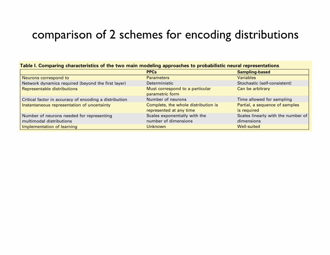
comparison of 2 schemes for encoding distributions
Box 2. Probabilistic representational schemes for inference and learning
Representing uncertainty associated with sensory stimuli requiresneurons to represent the probability distribution of the environmentalvariables that are being inferred. One class of schemes calledprobabilistic population codes (PPCs) assumes that neurons corre-spond to parameters of this distribution (Figure Ia). A simple buthighly unfeasible version of this scheme would be if different neuronsencoded the elements of the mean vector and covariance matrix of amultivariate Gaussian distribution. At any given time, the activities ofneurons in PPCs provide a complete description of the distribution bydetermining its parameters, making PPCs and other parametricrepresentational schemes particularly suitable for real-time inference[80–82]. Given that, in general, the number of parameters required tospecify a multivariate distribution scales exponentially with thenumber of its variables, a drawback of such schemes is that thenumber of neurons needed in an exact PPC representation would beexponentially large and with fewer neurons the representationbecomes approximate. Characteristics of the family of representableprobability distributions by this scheme are determined by thecharacteristics of neural tuning curves and noisiness [16] (Table I).
An alternative scheme to represent probability distributions inneural activities is based on each neuron corresponding to one of theinferred variables. For example, each neuron can encode the value ofone of the variables of a multivariate Gaussian distribution. Inparticular, the activity of a neuron at any time can represent a samplefrom the distribution of that variable and a ‘‘snapshot’’ of the activitiesof many neurons therefore can represent a sample from a high-dimensional distribution (Figure Ib). Such a representation requirestime to take multiple samples (i.e. a sequence of firing ratemeasurements) for building up an increasingly reliable estimate ofthe represented distribution which might be prohibitive for on-lineinference, but it does not require exponentially many neurons and —given enough time — it can represent any distribution (Table I). Afurther advantage of collecting samples is that marginalization, animportant case of computing integrals that infamously plaguepractical Bayesian inference, learning and decision-making, becomesa straightforward neural operation. Finally, although it is unclear howprobabilistic learning can be implemented with PPCs, sampling basedrepresentations seem particularly suitable for it (see main text).
Figure I. Two approaches to neural representations of uncertainty in the cortex. (a) Probabilistic population codes rely on a population of neurons that are tuned to thesame environmental variables with different tuning curves (populations 1 and 2, colored curves). At any moment in time, the instantaneous firing rates of these neurons(populations 1 and 2, colored circles) determine a probability distribution over the represented variables (top right panel, contour lines), which is an approximation ofthe true distribution that needs to be represented (purple colormap). In this example, y1 and y2, are independent, but in principle, there could be a single population withneurons tuned to both y1 and y2. However, such multivariate representations require exponentially more neurons (see text and Table I). (b) In a sampling basedrepresentation, single neurons, rather than populations of neurons, correspond to each variable. Variability of the activity of neurons 1 and 2 through time representsuncertainty in environmental variables. Correlations between the variables can be naturally represented by co-variability of neural activities, thus allowing therepresentation of arbitrarily shaped distributions.
Table I. Comparing characteristics of the two main modeling approaches to probabilistic neural representationsPPCs Sampling-based
Neurons correspond to Parameters VariablesNetwork dynamics required (beyond the first layer) Deterministic Stochastic (self-consistent)Representable distributions Must correspond to a particular
parametric formCan be arbitrary
Critical factor in accuracy of encoding a distribution Number of neurons Time allowed for samplingInstantaneous representation of uncertainty Complete, the whole distribution is
represented at any timePartial, a sequence of samplesis required
Number of neurons needed for representingmultimodal distributions
Scales exponentially with thenumber of dimensions
Scales linearly with the number ofdimensions
Implementation of learning Unknown Well-suited
Review Trends in Cognitive Sciences Vol.14 No.3
126
Berkes et al, Science 2011
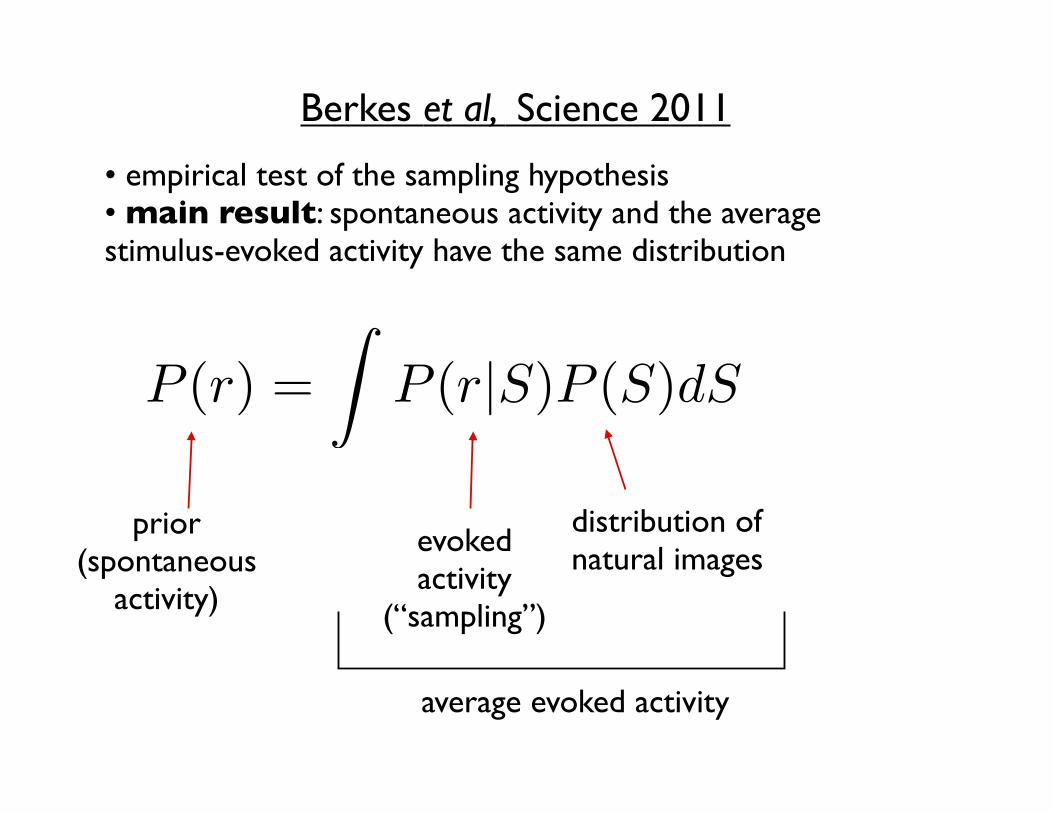
• empirical test of the sampling hypothesis• main result: spontaneous activity and the average stimulus-evoked activity have the same distribution
Berkes et al, Science 2011
• empirical test of the sampling hypothesis• main result: spontaneous activity and the average stimulus-evoked activity have the same distribution
prior(spontaneous
activity)
distribution of natural imagesevoked
activity(“sampling”)
average evoked activity
Berkes et al, Science 2011
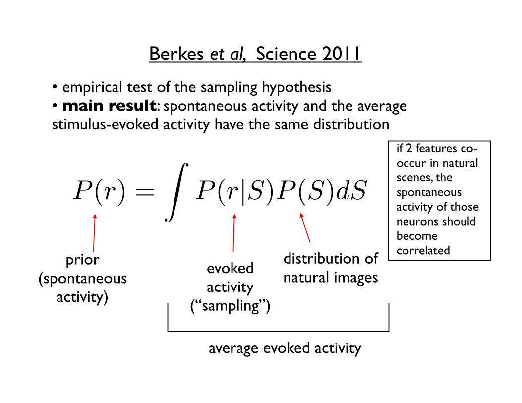
• empirical test of the sampling hypothesis• main result: spontaneous activity and the average stimulus-evoked activity have the same distribution
prior(spontaneous
activity)
distribution of natural imagesevoked
activity(“sampling”)
average evoked activity
if 2 features co-occur in natural scenes, the spontaneous activity of those neurons should become correlated
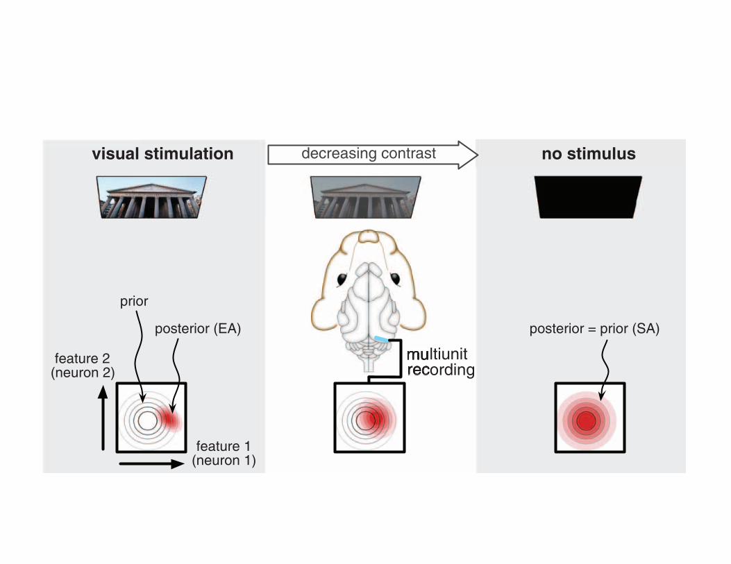
Fig. 1. Assessing the statistical optimality of theinternal model in the visual cortex. (A) The pos-terior distribution represented by EA (bottom, red-filled contours show pairwise activity distributions)in response to a visual stimulus (top) is increasinglydominated by the prior distribution (bottom, graycontours) as brightness or contrast is decreasedfrom maximum (left) to lower levels (center). In theabsence of stimulation (right), the posterior con-verges to the prior, and thus, SA recorded in dark-ness represents this prior. (B) Multiunit activityrecorded in V1 of awake, freely viewing ferretseither receiving no stimulus (middle) or viewingnatural (top) or artificial stimuli (bottom) is used toconstruct neural activity distributions in young andadult animals. Under natural and artificial stimuliconditions, EA distributions represent distributionsof visual features (red and green panels) inferredfrom particular stimuli. Average EA distributions(aEA) evoked by different stimuli ensembles arecompared with the distribution of SA recorded indarkness (black panels), representing the prior ex-pectations about visual features. Quantifying thedissimilarity between the SA distribution and theaEA distribution reveals the level of statistical ad-aptation of the internal model to the stimulus en-semble. The internal model of young animals (left)is expected to show little adaptation to the naturalenvironment and thus aEA for natural (and also forartificial) scenes should be different from SA. Adultanimals (right) are expected to be adapted to naturalscenes and thus to exhibit a high degree of similaritybetween SA and natural stimuli–aEA, but notbetween SA and artificial stimuli–aEA.
YOUNG ADULT
SIMILAR
prior (SA) prior (SA)no stimulus
average posterior (aEA)average posterior (aEA)
average posterior (aEA) average posterior (aEA)
natural stimuli
artificial stimuli
DIFFERENT
DIFFERENT DIFFERENT
visual stimulation no stimulusdecreasing contrastA
B
multiunit feature 2recording(neuron 2)
feature 1(neuron 1)
feature 2(neuron 2)
feature 1(neuron 1)
prior
posterior = prior (SA)posterior (EA)
development
7 JANUARY 2011 VOL 331 SCIENCE www.sciencemag.org84
REPORTS
on
Mar
ch 8
, 201
1w
ww
.sci
ence
mag
.org
Dow
nloa
ded
from
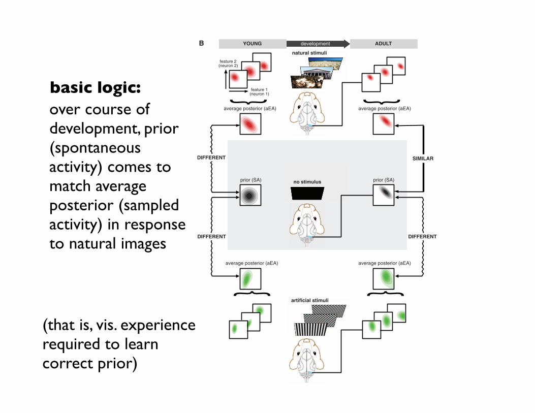
basic logic:over course of development, prior (spontaneous activity) comes to match average posterior (sampled activity) in response to natural images
(that is, vis. experience required to learn correct prior)
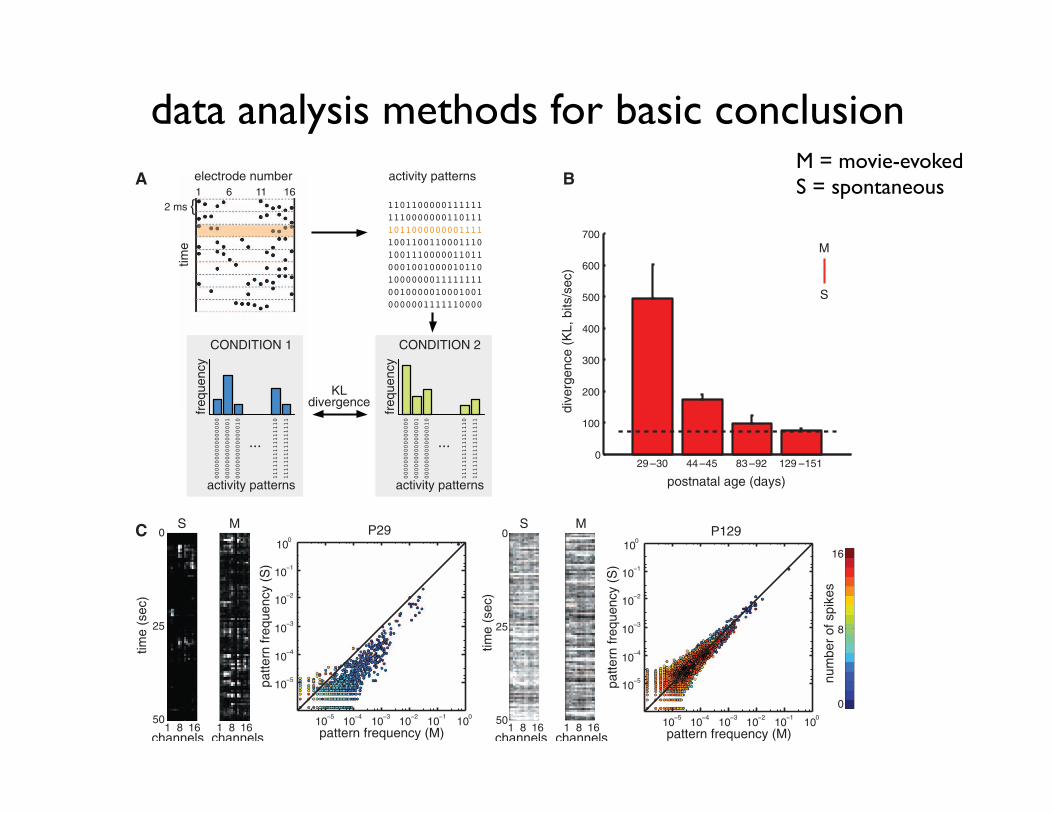
data analysis methods for basic conclusion
models. Yet identifying the neural correlates of op-timal internal models has remained a challenge(see supporting online text).
We addressed this problem by relating evokedand spontaneous neural activity (EA and SA, re-spectively) (9) to two key aspects of Bayesiancomputations performed with the internal model(Fig. 1A). The first key aspect is that a statisticallyoptimal internal model needs to represent its in-ferences as a probability distribution, the Bayesianposterior P(features|input, model) (2, 10) describ-ing the inferred probability that a particular com-bination of features may underlie the input. Thus,under the general assumption that the visual corteximplements such an optimal internal model, EAshould represent the posterior probability distri-bution for a given input image (2, 11, 12), and SAshould represent the posterior distribution elicitedby a blank stimulus. The second key aspect of astatistically optimal internal model, under onlymild assumptions about its structure, is that theposterior represented by SA converges to the priordistribution, which describes prior expectationsabout the frequency with which any given com-bination of features may occur in the environ-ment, P(features|model). This is because as thebrightness or contrast of the visual stimulus isdecreased, inferences about the features present
in the input will be increasingly dominated bythese prior expectations (for a formal derivation,see supporting online text). This effect has beendemonstrated in behavioral studies (3, 13), and itis also consistent with data on neural responses inthe primary visual cortex (V1) (14). Relating EAand SA to the posterior and prior distributionsprovides a complete, data-driven characterizationof the internal model without making strongtheoretical assumptions about its precise nature.
Crucially, this interpretation of the EA and SAdistributions allowed us to assess statistical opti-mality of the internal model with respect to an en-semble of visual inputs, P(input), using a standardbenchmark of the optimality of statistical models(Fig. 1B) (15). A statistical model of visual inputsthat is optimally adapted to a stimulus ensemblemust have prior expectations that match the actualfrequency with which it encounters different visualfeatures in that ensemble (16). The degree of mis-match can be quantified as the divergence betweenthe average posterior and the prior:
Div½⟨Pðfeaturesjiput,modelÞ⟩PðinputÞ∥ PðfeaturesjmodelÞ$ ð1Þ
where the angular brackets indicate averagingover the stimulus ensemble. A well-calibrated
model will predict correctly the frequency of fea-ture combinations in actual visual scenes, leadingto a divergence close to zero. However, if themodel is not adapted, or it is adapted to a differentstimulus ensemble from the actual test ensemble,then a large divergence is expected. As we iden-tified EA and SA with the posterior and priordistributions of the internal model, the statisticaloptimality of neural responses with respect to astimulus ensemble can be quantified by applyingEq. 1 to neural data, i.e., by computing the di-vergence between the average distribution of multi-neural EA (aEA), collected in response to stimulisampled from the stimulus ensemble, and the dis-tribution of SA (17) (Fig. 2A).
Because the internal model of the visual cortexneeds to be adapted to the statistical properties ofnatural scenes, Eq. 1 should yield a low diver-gence between aEA for natural scenes and SA inthe mature visual system. We therefore measuredthe population activity within the visual cortex ofawake, freely viewing ferrets in response to natural-scene movies (aEA) and in darkness (SA) at fourdifferent developmental stages: after eye opening atpostnatal day 29 (P29) to P30, after thematurationof orientation tuning and long-range horizontalconnections at P44 to P45 (18), and in two groupsof mature animals at P83 to P90 and P129 to P151
Fig. 2. Improving matchbetween aEA and SA overdevelopment. (A) Spikeswere recorded on 16 elec-trodes, divided intodiscrete2-ms bins, and convertedto binary strings, so thateach string described theactivity pattern of cells at agiven time point (top). Foreach condition, the histo-gram of activity patternswas constructed, and dif-ferent histograms werecompared by measuringtheir divergence (bottom).(B) Divergence betweenthe distributions of activitypatterns in movie-aEA (M)and SA (S), as a function ofage (red bars). As a ref-erence, the dashed lineshows the average of thewithin-condition baselinescomputed with within-condition data split intotwo halves (fig. S1). (C)Frequency of occurrenceof activity patterns underSA (S, y axis) versusmovie-aEA (M, x axis) in a young(left) and adult (right)animal. Each dot repre-sents one of the 216 =65,536 possible binaryactivity patterns; color code indicates number of spikes. Black line shows equality. The panels at the left of the plots show examples of neural activity on the 16electrodes in representative SA and movie-aEA trials for the same animals. Error bars on all figures represent SEM.
freq
uenc
y
29 30 44 45 83 92 129 1510
100
200
300
400
500
600
700
postnatal age (days)
dive
rgen
ce (
KL,
bits
/sec
)
M
S
electrode numbertim
e
{2 ms
activity patterns1 6 11 16
CONDITION 1
C
A B
activity patterns
KL
10 5 10 4 10 3 10 2 10 1 100
pattern frequency (M)
10 5
10 4
10 3
10 2
10 1
100
patte
rn fr
eque
ncy
(S)
P129
time
(sec
)
0
8
16
num
ber
of s
pike
s
10 5 10 4 10 3 10 2 10 1 100
pattern frequency (M)
10 5
10 4
10 3
10 2
10 1
100
patte
rn fr
eque
ncy
(S)
P29S
channels
M
channels channels
time
(sec
)
S
channels
M0
25
501 8 16 1 8 16
0
25
501 8 16 1 8 16
www.sciencemag.org SCIENCE VOL 331 7 JANUARY 2011 85
REPORTS
on
Mar
ch 8
, 201
1w
ww
.sci
ence
mag
.org
Dow
nloa
ded
from
M = movie-evokedS = spontaneous

contributions of spatial and temporal correlations
(n = 16 animals in total, table S1). The divergencebetween aEA and SA decreased with age (Fig. 2,B and C, Spearman’s r = –0.70, P < 0.004), andthe two distributionswere not significantly differentin mature animals (fig. S1, P83 to P90:m = 5.74,P = 0.11; P129 to P151: m = 2.03, P = 0.25).
What aspects of aEA and SA are responsiblefor their improvingmatch with age? Redundancyreduction, one prominent assumption regardingneural coding (19), would predict that neurons
behave as sparse (20, 21) and uncorrelated in-formation channels (22). To assess the importanceof correlations between the activities of differentneurons, we constructed surrogate distributions foraEA and SA that preserved single-neuron firingrates but otherwise assumed that neurons firedindependently (17). Thus, any divergence betweena real and a surrogate distribution must be due tocorrelated neural activities of second (23) or higherorder. By computing this divergence, we found
that the activity of neurons in both aEA and SAbecame increasingly correlated (Fig. 3A, Spearman’sr = 0.73, P < 0.002 for both curves) and in-creasingly nonsparse with age (fig. S2), which ar-gues against redundancy reduction.Moreover, theseincreasing correlations were important for thematchbetween aEA and SA because the surrogate SA didnot converge to the true aEA (Fig. 3B, Spearman’sr = 0.34, P = 0.22), excluding the possibility thatthe decreasing divergence between aEA and SA
Fig. 3. Contribution of spatial and temporal cor-relations to the match between aEA and SA. (A andB) The role of spatial correlations was quantified bythe divergence between the measured distributionsof neural activity patterns, movie-aEA (M) and SA(S), and the surrogate versions of the same distribu-tions (M̃ and S̃), in which correlations between chan-nels were removed, while the firing rates were keptintact (17). (A) The divergence between the measuredand surrogate distributions increased significantlyover age for both movie-aEA (orange) and SA (gray).(B) Enhanced match between movie-aEA and SA overdevelopment (red, compare Fig. 2B) disappearedwhen spatial correlations were removed from SA (pink).(C and D) Divergence of transition probability distribu-tions between measured neural activity patterns andtheir surrogate versions, in which temporal correlationswere removed, while firing rates and spatial correla-tions were kept intact (17). (C) Temporal correlations inadult animals (P129 to P151) as a function of the timeinterval, t. Within-condition divergences (top) showthat temporal correlations decreased with time lag inboth movie-aEA (orange) and SA (gray). Across-condition comparison (bottom) of the divergence ofaEA from themeasured SA (red) and from the surrogateSA (pink) shows that temporal correlations in the twoconditions were matched up to time intervals whenthey decayed to zero. (D) Temporal correlations at theshortest time interval (t = 2 ms) as a function of age.The match of transition probabilities between movie-aEA and SA improved (red). Removing temporalcorrelations from SA eliminated this match (pink). Inall figures, *P < 0.05, **P < 0.01, ***P < 0.001, m test (17).
0
200
400
2 4 6 10 20 40 100 10000
200
400
(msec) postnatal age (days)
postnatal age (days) postnatal age (days)
dive
rgen
ce (
KL,
bits
/sec
)
dive
rgen
ce (
KL,
bits
/sec
)di
verg
ence
(K
L, b
its/s
ec)
dive
rgen
ce (
KL,
bits
/sec
)
**
**
**
** ***
***
M
S
S~
M~
C D
A BM
S
S~
M~
M
S
S~
M
S
S~500
400
300
200
100
029-30 44-45 83-92 129-151
29-30 44-45 83-92 129-15129-30 44-45 83-92 129-151
1400
1200
1000
800
600
400
200
0
1200
1000
800
600
400
200
0
Fig. 4. Similarity be-tween aEA and SA isspecific to natural scenes.(A) Divergence betweenneural activity patternsevoked by different stimu-lus ensembles (movie-aEA:red, M; noise-aEA: blue,N; gratings-aEA: green,G) and those observed inSA. In adult animals, SAwas significantly moresimilar tomovie-aEA thannoise-aEA or gratings-aEA.(B) Two-dimensional projection of all neural activity distributions. Each dotrepresents one activity distribution in a different animal, colors indicate stim-ulus ensembles (movie-aEA: red, M; noise-aEA: blue, N; gratings-aEA: green,G; SA: black, S), intensity indicates age group (in order of increasing intensity:P29 to P30, P44 to P45, P83 to P92, and P129 to P151), ellipses delineatedistributions belonging to the same age group. Positions of dots werecomputed by multidimensional scaling (MDS) to be maximally consistent withpairwise divergences between distributions. Movie-aEAs were defined to be at
the origin. For young animals (faintest colors), SA was significantly dissimilarfrom all aEA distributions. In the course of development, SA moved closer toall aEAs; but by P129 to P151, SA was significantly more similar to movie-aEAthan artificial stimuli–aEAs, as quantified in (A). (C) Divergences measureddirectly between different aEA distributions (noise-aEA and movie-aEA: ma-genta, gratings-aEA and movie-aEA: yellow, gratings-aEA and noise-aEA:cyan) showed no decrease in the specificity of the responses to differentstimulus ensembles.
+
*
**
M
S
GN
A B C
M
N G
postnatal age (days) postnatal age (days)MDS dim 1 (a.u.)
MD
S d
im 2
(a.
u.)
div
erge
nce
(KL,
bits
/sec
)
div
erge
nce
(KL,
bits
/sec
)
500
400
300
200
100
0
500
600
700
400
300
200
100
029-30 44-45 83-92 129-15129-30 44-45 83-92 129-151
MNGS
-0.5 -0.4 -0.3 -0.2 -0.1 0 0.1
0.2
0.1
0
-0.1
-0.2
-0.3
-0.4
7 JANUARY 2011 VOL 331 SCIENCE www.sciencemag.org86
REPORTS
on
Mar
ch 8
, 201
1w
ww
.sci
ence
mag
.org
Dow
nloa
ded
from
M = movie-evokedS = spontaneous~ = shuffled
more spatial structurewith age
diff grows for shuffled data
temporal corrs
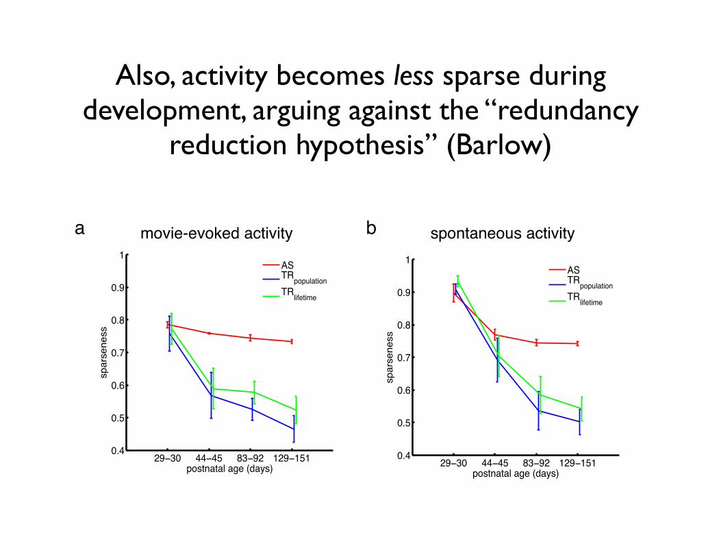
Also, activity becomes less sparse during development, arguing against the “redundancy
reduction hypothesis” (Barlow)
!"!#$ %%!%& '#!"! (!"!(&($)%
$)&
$)*
$)+
$)'
$)"
(
,-./01/12314536718.9
.,1:.505..
3
3
;<=>
,-,?21/@-0
=>2@A5/@B5
a b
!"!#$ %%!%& '#!"! (!"!(&($)%
$)&
$)*
$)+
$)'
$)"
(
,-./01/12314536718.9
.,1:.505..
3
3
;<=>
,-,?21/@-0
=>2@A5/@B5
movie-evoked activity spontaneous activity
Fig. S2: Sparseness of neural representations over development. Changes over developmentof three measures of sparseness: activity sparseness (AS, red), population sparseness(TRpopulation, blue), and lifetime sparseness (TRlifetime, green), as defined in Methods. All threemeasures decreased significantly over development, both for movie-evoked activity (activitysparseness: Spearman’s ρ = −0.79, P = 0.0004; population sparseness: ρ = −0.75, P = 0.001;lifetime sparseness: ρ = −0.65, P = 0.009), and spontaneous activity (activity sparseness:Spearman’s ρ = −0.61, P = 0.01; population sparseness:ρ = −0.78, P = 0.0006; lifetimesparseness: ρ = −0.75, P = 0.001). Thus, neural activity distributions became less sparse as theinternal model adapted to natural image statistics (Fig. 2B in main text), in contrast to the trendpredicted by sparse coding models (S10). See Methods for details.
16
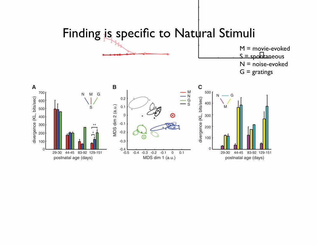
Finding is specific to Natural Stimuli
(n = 16 animals in total, table S1). The divergencebetween aEA and SA decreased with age (Fig. 2,B and C, Spearman’s r = –0.70, P < 0.004), andthe two distributionswere not significantly differentin mature animals (fig. S1, P83 to P90:m = 5.74,P = 0.11; P129 to P151: m = 2.03, P = 0.25).
What aspects of aEA and SA are responsiblefor their improvingmatch with age? Redundancyreduction, one prominent assumption regardingneural coding (19), would predict that neurons
behave as sparse (20, 21) and uncorrelated in-formation channels (22). To assess the importanceof correlations between the activities of differentneurons, we constructed surrogate distributions foraEA and SA that preserved single-neuron firingrates but otherwise assumed that neurons firedindependently (17). Thus, any divergence betweena real and a surrogate distribution must be due tocorrelated neural activities of second (23) or higherorder. By computing this divergence, we found
that the activity of neurons in both aEA and SAbecame increasingly correlated (Fig. 3A, Spearman’sr = 0.73, P < 0.002 for both curves) and in-creasingly nonsparse with age (fig. S2), which ar-gues against redundancy reduction.Moreover, theseincreasing correlations were important for thematchbetween aEA and SA because the surrogate SA didnot converge to the true aEA (Fig. 3B, Spearman’sr = 0.34, P = 0.22), excluding the possibility thatthe decreasing divergence between aEA and SA
Fig. 3. Contribution of spatial and temporal cor-relations to the match between aEA and SA. (A andB) The role of spatial correlations was quantified bythe divergence between the measured distributionsof neural activity patterns, movie-aEA (M) and SA(S), and the surrogate versions of the same distribu-tions (M̃ and S̃), in which correlations between chan-nels were removed, while the firing rates were keptintact (17). (A) The divergence between the measuredand surrogate distributions increased significantlyover age for both movie-aEA (orange) and SA (gray).(B) Enhanced match between movie-aEA and SA overdevelopment (red, compare Fig. 2B) disappearedwhen spatial correlations were removed from SA (pink).(C and D) Divergence of transition probability distribu-tions between measured neural activity patterns andtheir surrogate versions, in which temporal correlationswere removed, while firing rates and spatial correla-tions were kept intact (17). (C) Temporal correlations inadult animals (P129 to P151) as a function of the timeinterval, t. Within-condition divergences (top) showthat temporal correlations decreased with time lag inboth movie-aEA (orange) and SA (gray). Across-condition comparison (bottom) of the divergence ofaEA from themeasured SA (red) and from the surrogateSA (pink) shows that temporal correlations in the twoconditions were matched up to time intervals whenthey decayed to zero. (D) Temporal correlations at theshortest time interval (t = 2 ms) as a function of age.The match of transition probabilities between movie-aEA and SA improved (red). Removing temporalcorrelations from SA eliminated this match (pink). Inall figures, *P < 0.05, **P < 0.01, ***P < 0.001, m test (17).
0
200
400
2 4 6 10 20 40 100 10000
200
400
(msec) postnatal age (days)
postnatal age (days) postnatal age (days)
dive
rgen
ce (
KL,
bits
/sec
)
dive
rgen
ce (
KL,
bits
/sec
)di
verg
ence
(K
L, b
its/s
ec)
dive
rgen
ce (
KL,
bits
/sec
)
**
**
**
** ***
***
M
S
S~
M~
C D
A BM
S
S~
M~
M
S
S~
M
S
S~500
400
300
200
100
029-30 44-45 83-92 129-151
29-30 44-45 83-92 129-15129-30 44-45 83-92 129-151
1400
1200
1000
800
600
400
200
0
1200
1000
800
600
400
200
0
Fig. 4. Similarity be-tween aEA and SA isspecific to natural scenes.(A) Divergence betweenneural activity patternsevoked by different stimu-lus ensembles (movie-aEA:red, M; noise-aEA: blue,N; gratings-aEA: green,G) and those observed inSA. In adult animals, SAwas significantly moresimilar tomovie-aEA thannoise-aEA or gratings-aEA.(B) Two-dimensional projection of all neural activity distributions. Each dotrepresents one activity distribution in a different animal, colors indicate stim-ulus ensembles (movie-aEA: red, M; noise-aEA: blue, N; gratings-aEA: green,G; SA: black, S), intensity indicates age group (in order of increasing intensity:P29 to P30, P44 to P45, P83 to P92, and P129 to P151), ellipses delineatedistributions belonging to the same age group. Positions of dots werecomputed by multidimensional scaling (MDS) to be maximally consistent withpairwise divergences between distributions. Movie-aEAs were defined to be at
the origin. For young animals (faintest colors), SA was significantly dissimilarfrom all aEA distributions. In the course of development, SA moved closer toall aEAs; but by P129 to P151, SA was significantly more similar to movie-aEAthan artificial stimuli–aEAs, as quantified in (A). (C) Divergences measureddirectly between different aEA distributions (noise-aEA and movie-aEA: ma-genta, gratings-aEA and movie-aEA: yellow, gratings-aEA and noise-aEA:cyan) showed no decrease in the specificity of the responses to differentstimulus ensembles.
+
*
**
M
S
GN
A B C
M
N G
postnatal age (days) postnatal age (days)MDS dim 1 (a.u.)
MD
S d
im 2
(a.
u.)
div
erge
nce
(KL,
bits
/sec
)
div
erge
nce
(KL,
bits
/sec
)
500
400
300
200
100
0
500
600
700
400
300
200
100
029-30 44-45 83-92 129-15129-30 44-45 83-92 129-151
MNGS
-0.5 -0.4 -0.3 -0.2 -0.1 0 0.1
0.2
0.1
0
-0.1
-0.2
-0.3
-0.4
7 JANUARY 2011 VOL 331 SCIENCE www.sciencemag.org86
REPORTS
on
Mar
ch 8
, 201
1w
ww
.sci
ence
mag
.org
Dow
nloa
ded
from
M = movie-evokedS = spontaneousN = noise-evokedG = gratings

Conclusions
evoked activity
stimulus-dependentP (r|y)
stimulus-averaged�P (r|y)P ∗(y) dy
spon
tane
ous
activ
ity
ignored“classical” neural coding(e.g., Rieke et al., 1997 )information transmission
Schneidman et al., 2006error correction
analyzedP (r)
Luczak et al., 2009coding robustness
this paperprobabilistic inference
Table S2: Approaches to neural activity analysis. Our approach assesses the statistical
optimality of an internal model for probabilistic inference and therefore it is conceptually
different from standard approaches in neural coding that focus on the optimality of information
transmission in a neural circuit by quantifying how easily a stimulus, y can be recovered from the
evoked neural responses, r (S33, S34). To provide a statistical description of the mapping between
stimuli and EA responses, standard neural coding analyses focus on responses to individual
stimuli (left column). These approaches either compute the average stimulus eliciting a particular
EA pattern for constructing receptive fields by reverse correlation methods (S35), or characterize
the distribution of EA patterns in response to each individual stimuli, e.g. by computing its
average for constructing tuning curves (S36) or by computing higher order moments for
characterizing the roles of “noise” correlations in multi-neural responses (S37). In contrast, for
assessing the statistical optimality of an internal model, the average distribution of EA patterns
needs to be computed, where the average is taken over many individual stimuli sampled from a
particular stimulus ensemble, P ∗(y) (Fig. 1 in the main text). In addition, this distribution then
needs to be compared to the distribution of SA patterns (lower right). While averaged EA
distributions have been recently analysed to study the error correcting properties of EA patterns
(S38, upper right), SA has typically been excluded from such analyses. Recent analyses of SA
have been limited to comparing patterns of neural activity recorded during spontaneous activity
with those evoked by particular stimuli, finding similar structure and repeating motives (S39, S40,
lower left), but see also (S1).
20
• sampling is great
• interesting, surprising account of “what spontaneous activity means”
• key prediction: spontaneous activity matches average evoked activity
• match gets better during development (learning story: “prior is being tuned to average posterior”)
Conclusions
• sampling is great
• interesting, surprising account of “what spontaneous activity means”
• key prediction: spontaneous activity matches average evoked activity
• match gets better during development (learning story: “prior is being tuned to average posterior”)
open question• are there other stories consistent with the fact that the
average evoked activity has the same distribution as spontaneous activity?
Conclusions