Embed Size (px)
Citation preview
STATISTICALLY MONITORING INVENTORY ACCURACY IN
LARGE WAREHOUSE AND RETAIL ENVIROMENTS
by
ANDREW HUSCHKA
A THESIS
Submitted in partial fulfillment of the requirements for the degree
MASTER OF SCIENCE
Department of Industrial and Manufacturing Systems Engineering
College of Engineering
KANSAS STATE UNIVERSITY Manhattan, Kansas
2011
Approved By: Major Professor
John English

Abstract
This research builds upon previous efforts to explore the use of Statistical Process Control (SPC)
in lieu of cycle counting. Specifically a three pronged effort is developed. First, in the work of Huschka
(2009) and Miller (2008), a mixture distribution is proposed to model the complexities of multiple Stock
Keeping Units (SKU) within an operating department. We have gained access to data set from a large
retailer and have analyzed the data in an effort to validate the core models. Secondly, we develop a
recursive relationship that enables large samples of SKUs to be evaluated with appropriately with the
SPC approach. Finally, we present a comprehensive set of type I and type II error rates for the SPC
approach to inventory accuracy monitoring.

iii
Table of Contents
List of Figures ................................................................................................................................................ v
List of Tables ................................................................................................................................................ vi
Acknowledgements .................................................................................................................................... vii
Chapter 1 – Introduction and Objective ...................................................................................................... 1
1.1 Background ......................................................................................................................................... 1
1.2 Objectives ............................................................................................................................................ 3
1.3 Task ..................................................................................................................................................... 4
Chapter 2 – Literature Review ..................................................................................................................... 5
2.1 Inventory Control Systems .................................................................................................................. 5
2.1.1 Cycle Counting ........................................................................................................................ 8
2.1.1.1 Random Sample Cycle Counting ............................................................................. 7
2.1.1.2 Geographic Cycle Counting ..................................................................................... 7
2.1.1.3 Process Control Cycle Counting .............................................................................. 8
2.1.1.4 ABC Method ............................................................................................................ 8
2.2 Statistical Process Control ................................................................................................................. 10
2.2.1 Control Charts ....................................................................................................................... 11
2.2.2 Type I and Type II Error Rates for Control Charts ................................................................. 12
2.2.3 Average Run Length (ARL) .................................................................................................... 12
2.2.4 Variable Control Charts ......................................................................................................... 14
2.2.4.1 Control Chart .................................................................................................... 14
2.2.4.2 R Control Chart ..................................................................................................... 16
2.2.5 Attribute Control Charts ....................................................................................................... 18
2.2.5.1 P Control Chart ..................................................................................................... 19
2.2.5.2 C Control Chart ..................................................................................................... 22
2.3 Background of SPC Approach for Inventory Control ......................................................................... 23
2.3.1 Application and Notation ...................................................................................................... 24
2.3.2 SPC Approach to Inventory Accuracy Monitoring ................................................................ 26
2.3.3 Constructing an Example ...................................................................................................... 27
Chapter 3 – Defining Sub-populations of SKUs ......................................................................................... 29
3.1 Defining Sub-Populations .................................................................................................................. 29
iv
3.2 Experimentwise Error Rate ............................................................................................................... 33
Chapter 4 – Computer Program ................................................................................................................. 34
4.1 Defining Recursive Relationship ........................................................................................................ 34
4.3 Computer Program Setup ................................................................................................................. 35
Chapter 5 – Type I Error Rates ................................................................................................................... 37
5.1 Defining and Values ................................................................................................................... 37
5.2 Type I Error Rate Results .................................................................................................................. 39
5.3 Type I Error Rate Conclusions ........................................................................................................... 41
Chapter 6 – Type II Error Rates .................................................................................................................. 43
6.1 Type II Error Rates Shift .................................................................................................... 43
6.2 Type II Error Rates Shift .................................................................................................... 45
6.3 Type II Error Rates Shift .................................................................................................... 47
6.4 Type II Error Rate Conclusion ............................................................................................................ 50
Chapter 7 – Conclusions and Future Work ................................................................................................ 52
7.1 Conclusions ....................................................................................................................................... 52
7.2 Future Work ..................................................................................................................................... 53
References ................................................................................................................................................. 55
Appendix A – Computer Program .............................................................................................................. 58
Appendix B – , , and m Values for Tables ............................................................................................ 63
Appendix C – All Type I Error Rate Tables ................................................................................................. 65
Appendix D – All Type II Error Rate Tables ................................................................................................ 68

v
List of Figures
Figure 1: Pareto Principle Example ............................................................................................................... 9
Figure 2: Discount Department Store ......................................................................................................... 24
Figure 3: Discount Department Stores ( and ) ..................................................................................... 25
Figure 4: Home Electronics t-test Matrix ................................................................................................... 30
Figure 5: Computer Program Output ......................................................................................................... 36

vi
List of Tables
Table 1: Complete Enumeration Example ................................................................................................. 28
Table 2: Game Sub-Population .................................................................................................................. 31
Table 3: Home Electronics Sub-Population ................................................................................................ 31
Table 4: Accessories Sub-Population .......................................................................................................... 31
Table 5: Ink Sub-Population ........................................................................................................................ 32
Table 6: Computer Sub-Population ............................................................................................................ 32
Table 7: Ink Sub-Population ........................................................................................................................ 32
Table 8: Complete Enumeration vs. Computer Program............................................................................ 36
Table 9: Flat Min/Max Type I Error Rates ................................................................................................... 39
Table 10: Linear/Weighted Type I Error Rates ........................................................................................... 40
Table 11: Flat Min/Max, Type II Error Rates ............................................................................ 43
Table 12: Linear/ Weighted, Type II Error Rates ...................................................................... 44
Table 13: Flat Min/Max, Type II Error Rates ............................................................................ 45
Table 14: Linear/ Weighted, Type II Error Rates ...................................................................... 46
Table 15: Flat Min/Max, Type II Error Rates ............................................................................ 48
Table 16: Linear/ Weighted, Type II Error Rates ...................................................................... 48
Table 17: Flat Min CL vs. Shift CL ................................................................................................................ 50
Table 18: Flat Max CL vs. Shift CL................................................................................................................ 50

vii
Acknowledgements
The research completed for this thesis could not have been successful without the help of
numerous individuals. I want to start by thanking Dean John English who has served as my advisor
throughout the past two years of work on this thesis. Dean English provided support and always made
time in his busy schedule to assist in any way that he could. I have learned a great deal from Dean
English technically, academically, and general life lessons. I was fortunate to have the opportunity to
work so closely with Dean English and I know the knowledge and experience gained throughout this
time will stick with me perpetually.
Next, I want to thank Dr. Todd Easton for his work on the computer programming and recursive
function break through. Dr. Easton’s wide breadth of knowledge allowed him to easily understand the
problem. Dr. Easton was then able to apply his intelligence in computer programming to advise and
direct me in the creation of the computer program. During our time working together Dr. Easton was
again able to use his knowledge base to develop the breakthrough recursive function that is utilized in
the research. Dr. Easton has played an integral in this thesis and on my college career. I know that as I
move on many of his teachings will come into use.
Finally, I want to thank Dr. John Boyer and Kyle Huschka for the support they have provided. Dr.
Boyer serves on my defense committee and has provided help with his expertise in statistics. Dr. Boyer
has been willing to meet and help out in any way that I have needed. This thesis was an extension of
research completed by Kyle. During my time working on the thesis Kyle assisted in understanding his
work and also provided ideas to improve my work. All of these contributions have been invaluable to
the completion and success of this thesis.

1
Chapter 1: Introduction and Objectives
1.1 Background
Inventory record accuracy is vital to companies with high numbers of products. For a company to
have accurate records, actual on hand inventory should equal their recorded inventory. As retail stores
become larger and distribution centers service larger regions, assurance of accurate inventory records
becomes much more significant and a more challenging task. Retail environments (e.g. large retail
stores, distribution centers, etc.) often have thousands of different stock keeping units (SKU’s) in their
inventory. Brooks and Wilson (2005) state that failure to keep accurate inventory records can result in
loss of product, time wasted correcting records, product not in stock for consumers, and overstock of
items.
Cycle counting is currently the most common and established method used by companies to keep
inventory record accuracy as described in Dehoratius and Raman (2008). Cycle counting has generally
replaced periodic physical inventory checks. Cycle counting is accepted as a better method as it doesn’t
require the entire store or warehouse to shut down to count SKU’s. Physical inventory checks are not
only tedious and stressful, but they usually result in errors due to the time constraints on the availability
of the facility. With cycle counting, subsets of the SKU’s within inventory are examined to see if the
actual on hand inventory equals the recorded inventory. If there are differences between the two,
errors are corrected. Cycle counting is found to be less disruptive to daily operations, provides an
ongoing measure of inventory accuracy, and can be adapted to focus on items with higher value.
Brooks and Wilson (2005) explain that with the correct execution of cycle counting, a company can
have “95% or better accuracy.” The dilemma for a large company is that it takes a large amount of
resources, labor hours, and money to ensure that cycle counting is implemented correctly.

2
Consequently, for large retail environments, there is a need for a method to keep high levels of
inventory accuracy without the large amount of time and resources that cycle counting requires.
Furthermore, a more feasible approach would be one that is simply a monitoring approach and can be
added to the periodic activities of operational personnel. As companies strive to be more efficient, the
cost competitive pressures mount on the effective use of resources.
Statistical Process Control (SPC) is a proven statistical method used to monitor processes and
improve quality using variance reduction. SPC utilizes random samples to monitor and control a process
to ensure it is operating correctly and producing parts in accordance to its stochastic nature. In the
inventory accuracy domain there is an opportunity to utilize random samples rather than the prescribed
selection of SKU’s as implemented in varied approaches of cycle counting so that Type I and Type II
errors are controlled. As such, statistical process control is an ideal application for monitoring inventory
accuracy as the total sampled number of SKU’s can be dramatically reduced. There are two SPC tools
that could be used to monitor inventory record accuracy.
The first method is a P-chart. A P-chart can be used to monitor the percent of SKU’s in a sample for
which the observed inventory level that matches the recorded inventory level. This means a random
sample of n SKU’s is selected and each SKU is checked to see if the actual on hand inventory exactly
equals the recorded inventory. The number of SKU’s for which the observed quantity matches the
recorded inventory is divided by the total sample size. That provides a point estimate of the inventory
accuracy, or P. Over time, P, is plotted on a P chart as seen in Cozzucoli (2009). The second method is a
C-chart. C-charts can be used to monitor the collective number of item adjustments for a set of
randomly observed SKU’s where the on hand inventory failed to match the recorded inventory. That is,
when a given SKU is sampled and the on-hand inventory does not match the recorded inventory level,
the on-hand inventory or the recorded inventory will be adjusted in order to match the two. This means
that either items will be ordered or the on-hand inventory will be adjusted. For the C-chart application

3
to inventory accuracy an inspection unit of size n is sampled and the observed number of inventory
adjustments is plotted in relationship to time as seen in Huschka (2009).
Huschka (2009) presents an analytical approach for small sample sizes and a simulation to
provide suitable estimates of Type I and Type II errors for larger sample sizes as suggested in Yu (2007).
In this research, we establish an efficient approach so that Huschka’s (2009) analytical approach can be
extended to a wide set of real world scenarios. A program is created that allows for the examination of
type I and type II error rates of the C-chart with such populations. Conditions considered are typical of
populations found in the industry.
1.2 Objective
Recent advances in Huschka (2009) provide much of the motivation for this research. Huschka
(2009) presents an analytical approach to determining the Type I and Type II error rates for C-charts
used to detect shifts in the number of inventory adjustments. In this thesis, the objective is to
comprehensively explore the use of a C-chart to manage inventory adjustments that are required when
the recorded inventory fails to match the number of inventory on the shelf. The first part of our research
will verify the analytical model created by Huschka (2009) with real world data provided by a large
international retailer. As the work of Huschka (2009) is limited to small samples, we extend that work to
examine the impact of the C-chart approach in a real world setting.

4
1.3 Tasks
The following tasks are a summary of the goals of this research:
1. Verify Analytical Model
1.1. Work with a national leader in the retail environment to secure data that supports or refutes
the modeling concepts in Huschka (2009)
1.2. Analyze the data to determine “reasonable” modeling parameter values
1.3. Report findings of 1.1 and 1.2 in a report to document the usefulness of assuming the
environmental conditions as prescribed in Huschka (2009)
2. Create a program able to calculate any sample size
2.1. Define an equation able to calculate any sample size
2.2. Create program that allows for the evaluation of type I and type II error rates for different
values of the c chart as defined below. is the proportion of the population represented by
the PDF, is the Poisson arrival rate of the population, is number of SKU’s sampled, and is
the number of sub-populations
2.2.1.
2.2.2.
2.2.3.
2.2.4.
2.3. Using the large retail environment data to present observations and conclusions

5
Chapter 2: Literature Review
To understand this research, there are two fields of work that are important: statistical quality
control and inventory control. Specifically, we pay particular attention to the advances in the use and
development of statistical process control (SPC) and cycle counting. We provide basic descriptions of the
two areas and some of the more recent advances. It will be our observation that SPC can be used to
efficiently monitor inventory accuracy.
2.1 Inventory Control Systems
Inventory record accuracy is vital to any company with high levels of inventory. For a company to
keep accurate records, on hand inventory should equal recorded inventory. This has become a
challenging task for some environments (e.g. large retail stores, distribution centers, etc.) because they
often have thousands of different stock keeping units (SKU’s) in their inventory. Piasecki (2003) indicates
that there are several causes of discrepancies between actual on hand inventory and recorded
inventory: stock loss or shrinkage, transaction errors, and product misplacement. Kok and Shang (2007)
report that there are two problems that occur when inventory accuracy is poor. The first happens when
an out of stock item is reported as in stock. This prevents the replenishment system from ordering more
of the product. This results in higher backorder penalties and lost sales. The second happens when the
recorded inventory shows fewer items than are in the physical inventory. This causes more products to
be ordered and leads to higher inventory costs. To find and fix these discrepancies, there needs to be a
system to monitor and make the required changes to inventory records.

6
2.1.1 Cycle Counting
Dehoratius and Raman (2008) examine 370,000 inventory records from 37 different stores and
found that 65% of their inventory was inaccurate. This is not uncommon, and it is the reason that many
companies have implemented strategies to keep track of the inventory records. Cycle counting is
currently the most common and established method used by companies to keep inventory record
accuracy. Cycle counting generally replaces annual physical inventory checks. Cycle counting is accepted
as a better method, because it doesn’t require the entire store to shut down to count SKUs as often
required with physical inventory checks. Physical inventory checks are tedious and usually result in
errors due to the time constraints on counting the SKUs. With cycle counting, subsets of inventory are
counted to check that the actual on hand inventory equals the recorded inventory. If there are
differences between the two, errors are corrected. When compared to inventory checking where a
facility is closed and all SKUs are checked for accuracy, cycle counting is less disruptive to daily
operations, provides ongoing measure of inventory accuracy, and can be enhanced to focus on items
with higher monetary value.
Brooks and Wilson (2005) stated that “through the proper use of cycle counting, inventory
record accuracy above 95% can be consistently maintained.” As suggested, the dilemma for a large
company is that it takes a large amount of resources, labor hours, and money to ensure that cycle
counting is implemented correctly. For large environments, there is a need for a method to keep high
levels of inventory accuracy that does not require the large amount of time, structure of operation, and
large resources required by cycle counting. We further assume that basic concepts of statistical
inference can be accepted as basic knowledge of the work force. As companies strive to be more
efficient, cost competitive pressures mount on the effective use of resources. The next section provides
an overview of some of the more common ways that cycle counting is being performed. Most of the
concepts presented are found in Brooks and Wilson (2005).

7
2.1.1.1 Random Sample Cycle Counting
Random sample cycle counting is one of the more basic forms of cycle counting. SKU’s are
randomly selected for a given inventory such that each SKU of the population has an equal opportunity
of being selected. There are two ways that random cycle counting can be carried out. They are called
constant population counting and diminishing population counting.
Constant population technique implements sampling such that any SKU can be selected for any
sampling period. In essence, this is sampling with replacement and is similar to the concept of sampling
for SPC. This means, that if a SKU is picked for one sampling interval, it could be picked at the exact
same likelihood the next period. It is also called “sampling with replacement.” Diminishing population
implements sampling such that after a SKU is picked it isn’t returned to the population until all the other
SKU’s have been chosen. In essence this is “sampling without replacement.” Probabilistically, this is the
sampling approach connected to distributions such as the hypergeometric distribution.
2.1.1.2 Geographic Cycle Counting
Schreibfeder (2005) describes geographic cycle counting as starting at one end of the warehouse
and counting a certain number of products each day until you reach the other end of the building. This
method is considered the simplest form of cycle counting. This method allows a methodical approach to
counting all materials in a warehouse, and it is not confusing to implement. Schreibfeder (2005)
recommends that all items be counted at least once every 3 months.

8
2.1.1.3 Process Control Cycle Counting
Brooks and Wilson (2005) first introduced process control cycle counting. It is built upon the
examination of SKUs that are convenient to count. This method is considered controversial in theory but
effective in practice. To perform this method, the inventory records must have counts for each SKU at
each location where the SKU is stored. The employee is then sent to a specific location to perform the
cycle counting. They check the parts in every location, but they only spend time counting parts that will
be easy to count. They then make adjustments necessary as overages or shortages are discovered.
If the parts are not easy to count, the counter checks the part identification, location, and order
size. The employee then “eye balls” or estimates the number in a given the bin to see if it looks similar
to the number of parts recorded in the system. If there is a large discrepancy between the numbers of
parts in the bin compared to what the recorded inventory shows then a precise count is attained and an
adjustment is made. For example, if the bin has about 10 parts in it and the system records an inventory
of 100, the employee denotes the discrepancy, makes the exact count and the necessary adjustment.
Brooks and Wilson (2005) state that the advantage of this method is that you can count 10-20 times the
part numbers in a given time period with no extra cost. The disadvantage is having the employees
determine what is “easy to count”.
2.1.1.4 ABC Method
The ABC method, also known as the Ranking Method, is based on the Pareto Principle and is a
common way to perform cycle counting. The Pareto Principle has its root in economics where it is
known that a majority of the wealth is held by a few number of people. For application inventory
9
accuracy, it is assumed that only a few number of SKUs drive the bulk of inventory inaccuracy. An
example of the Pareto Principle can be seen below in Figure 1.
Figure 1: Pareto Principle Example (Reproduced from Inventory and Demand Analysis. <http://www.resourcesystemsconsulting.com/blog/archives/37>)
In Figure 1., inventory items are divided into three different categories: A items, B items, and C
items. The ABC method places emphasis on parts that have a history of poor accuracy levels. Figure 1
shows that although A items are only 20% of the total inventory, they result in 75% of the errors. It can
also be seen that B items are 30% of the total inventory and result in 15% of the total errors. Finally, C
items are 50% of the total inventory but result in only 10% of the total errors.
Rossetti et al. (2001) states that the ranking method can be tailored to the specific priorities of
the organization (e.g., accuracy levels, inventory cost, etc.). The company must establish the ranking of
each SKU and design sampling accordingly. Rossetti et al. (2001) warns that the ABC method has a
disadvantage in that the category classifications are primarily based on financial considerations. When
considering delaying production or shipments, inexpensive items are as important as expensive items.

10
For example in an automobile assembly plant, the engine is much more expensive than the motor
mounts, but absence of either stops production. Thus, it is important to consider lead-time, amount of
usage, and bill of material (BOM) level when employing ABC cycle counting.
2.2 Statistical Process Control (SPC)
Montgomery (2009) states that “a company must continuously seek to improve process
performance and reduce variability in key parameters.” He goes further to state “Statistical Process
Control (SPC) is a primary tool for achieving this objective.” SPC is a powerful collection of problem
solving tools useful in achieving process stability and improving capability through the reduction of
variability. SPC has become such a powerful tool because it is easy to use, it has a significant impact, and
can be applied to virtually any process. The tools of SPC are often called the “the magnificent seven”,
they are:
1. Histogram 2. Check Sheet 3. Pareto Chart 4. Cause and Effect Diagram 5. Defect Concentration Diagram 6. Scatter Diagram 7. Control Chart
For this research, we use control charts as a method to monitor inventory accuracy. Control
Charts utilize random samples to monitor a process to ensure it is operating in accordance to its natural
stochastic behavior. In inventory accuracy domain, there is opportunity to utilize random samples
rather than the various approaches of cycle counting. As eluded before, the random sample approach of
cycle counting hints at the procedures used in control charts. However, there is no statistical approach
to draw inference on the entire inventory. Control charts are statistically valid approaches that control
11
underlying type I and type II errors. Statistical process control is an ideal application for monitoring
inventory accuracy.
2.2.1 Control Charts
Control charts were first proposed in Shewart (1926, 1927), and they are considered one of the
primary techniques of SPC. A control chart essentially plots measurements of a quality characteristic
versus time. The chart consists of a centerline (CL) upper control limit (UCL) and lower control limit
(LCL). The centerline is used to describe the central tendency or estimate average of the sampled
statistic. The UCL and LCL denote the upper and lower bounds where the sampled statistic should fall
given the process is operating in its normal stationary way (also called “in-control”). The UCL and LCL
are estimated differently depending on the sampled statistic, but they all follow a similar formula which
can be seen below in equation (1) and (2):
(1)
(2)
In this case, w is the sampled statistic that measures a given quality characteristic. The mean of
w is , and the variance of w is . L is the distance of the control limits from the center line in
multiples of the standard deviation of w and is often assumed to be 3. From these equations it is noted
that the mean and variance are never known in practice and can only be estimated.

12
2.2.2 Type I and Type II Error Rates for Control Charts
Control limits are generally set at three (3) standard deviations away from the mean of the
population. When a data point falls out of these limits, it indicates that the process is not stationary or
out of control. There are two types of errors that are associated with control charts. They are type I and
type II errors. When predicting type I and type II errors, there is a null hypothesis ( ) and an alternative
hypothesis ( ). In our retail and warehouse domain the null hypothesis will be the mixture distribution
is representative of the population. The alternative hypothesis will be that the mixture distribution is not
representative of the population.
The type I ( ) errors are known as the false alarm rate and occurs when the null hypothesis is
rejected, but it is actually true. In application, this would happen if the operator concludes that the
process is out of control when it is in fact in control. Type II ( errors happen when we fail to reject the
null hypothesis but the alternative is actually true. This means that the operator concludes the process is
in control when it is in fact out of control. The common probabilistic statements defining and are
shown below in equation (3) and (4):
(3)
(4)
2.2.3 Average Run Length (ARL)
The average run length (ARL) is the average number of points that must be plotted before a
point indicates an out of control condition. For Shewart control chart, the ARL can be calculated from
the equation (5):

13
(5)
The probability that any point exceeds the upper control limit or falls below the lower control
limit is P. The in control ARL is the inverse of the probability of a type I error, . The out of control ARL is
the inverse of (1-P( )). The out of control ARL is the average number of points needed to detect a
process shift when one has occurred. The formulas to find type I and type II error rates are below in
equation (6) and (7):
(6)
(7)
In equation (6) and (7) W is the sampled statistic. The ARL is used in many research advances to
evaluate the performance of control charts. Crowder (1987) shows a numerical procedure using integral
equations for the tabulation of moments of run lengths of exponentially weighted moving averages
(EWMA). Gan (1993) presents a computer program for computing the probability of a function and
percentiles of run length for a CUSUM control chart. Calzada and Scariano (2003) study the integral
equation and Markov chain approaches for computing average run lengths for two-sided EWMA control
charts.
Crowder (1987) tabulates ’s for the EWMA control chart. Champ and Woodall (1987) use
Markov chains to compute the ARL’s for the chart while embedding various run rules. Marcellus
(2008) compares Bayesian analogue of Shewhart chart to cumulative sum charts. He found that
Bayesian offered better results, but it required more information which may be difficult to obtain.

14
Burroughs et al. (2003) studied the effect of using run rules on charts and determined that they
improve the sensitivity of the charts. There are hundreds of such advances in the literature, and they
point to the conclusion that controls charts, if designed correctly, can be useful in monitoring
performance. The ultimate goal of a control chart is to have a large in control ARL and small out of
control ARL’s.
2.2.4 Variable Control charts
Variable control charts are used when quality characteristics are expressed in terms of
numerical measurements. This can include any single measurable quality characteristic such as length,
weight, diameter, or volume. The three common control charts that are used for variable data are the ,
R, and S control Charts. The control chart is used to monitor the process average or mean quality level
and is also known as the control chart for means. The R control chart is used to monitor the range, while
the S control chart is used to monitor the standard deviation. The range is the difference between the
max and minimum values found in a given sample of n observations. Either the R or S control chart can
be used to monitor the process variability.
2.2.4.1 Control Chart
For a process, sampled observations, , can be collected. The observations are assumed to
follow a normal distribution with mean µ and variance . The sample average, called , (an unbiased
estimator of µ) is calculated as:
(8)
15
It is well known that the resulting population of s follows the normal distribution with mean µ
and variance (
). The control chart is used to monitor the ’s and gain inference on the stability
of the central tendency of the process. Using equations (1) and (2) as a basis, the theoretical control
limits for the chart are as follows:
(9)
(10)
(11)
Clearly, µ and are never known with certainty, so in practice they must be estimated with
unbiased estimators as shown below:
(12)
(13)
In equation (12) m = number of subgroups observed. d2 is one of many control chart constants
and are tabled for various subgroup sizes in all basic texts in quality control (e.g., Montgomery
(2009)). for each subgroup i, also called the range. The
resulting control limits used in practice are as follows:
(14)

16
(15)
(16)
Making the substitution,
, (also a standard tabled value for control charts), the
resulting control chart limits are classically estimated as:
(17)
(18)
(19)
2.2.4.2 R Control Chart
R and S charts are used to monitor process variability. The R chart does this by plotting the range
while the S chart uses the sample standard deviation. For this research, we are going to concentrate on
the R chart as a method to monitor process variability. As described earlier is simply the difference
between the largest and smallest observation and can be easily collected. The center line of an R chart is
the average range which can be calculated below:
(20)

17
The R chart follows the basic 3-sigma control limit approach, where and are the mean
and variance of the range statistic R as described in Montgomery (2009). Again using the theoretical
control limits from equation (1) and (2) the control limits are defined as:
(21)
(22)
(23)
Because, µ and are never known with certainty, so in practice they must be estimated with
unbiased estimators as shown below:
(24)
(25)
is another control chart constant and can be found in all basic texts in quality control (e.g.,
Montgomery (2009)). Substituting these unbiased estimators the resulting control limits used in practice
are as follows:
(26)
(27)
(28)
18
and are control chart constants whose values depend on the sample size. To ease the
computations equation (29) and (30) can be defined:
(29)
(30)
Substituting in these equations the resulting control chart limits are classically estimated as:
(31)
(32)
(33)
The R chart has been a very commonly used method for monitoring process variability. Wang
(2009) identifies the R chart as a hybrid approach that allows you to control chart concurrent patterns at
once. Castagliola (2005) found that the R chart can be used in tandem with a EWMA control chart to
better monitor the process range. Costa and Magalhaes (2007) shows how joint X and R charts with
varying sample sizes and variable intervals improves the control chart performance in terms of the
speed with which shifts can be detected.
2.2.5 Attribute Control Charts
19
Attribute control charts are the second way that data can be monitored by control charts. Unlike
variable control charts that are used to measure numerical data, attribute control charts are used to
measure values that are determined by a discrete response. Some examples of attribute control charts
would be conforming/nonconforming, pass/fail, go/no go, and good/bad. There are four different types
of attribute control charts that are commonly used and they are P, NP, C and U control charts. Each of
these charts will be explained in more detail in the following sections.
There are numerous other control charts that have been developed. Burke (1992) examines the
use of a G chart and H chart to monitor the total number of defects and average number of defects
based on the geometric distribution. Taleb (2009) looks at attribute control charts based on average run
length with a pre defined process shift. Rudisill et al. (2004) uses a method of modifying U charts to
monitor Poisson attribute processes. Ou et al. (2009) looks at using CUSUM as a method of control chart
for attribute controls. Woodall (1997) gives a good summary of substitutes that have been tried for P,
NP, C, and U charts. He goes further to explain why P, NP, C, and U are the widely accepted choice for
attribute charts. In this research we will concentrate on P and C control charts.
2.2.5.1 P Control Chart
The P chart is commonly called the fraction nonconforming control chart. A part is considered
nonconforming when it doesn’t “conform” to the standard or requirement of one or more
characteristics. Let us assume that the probability a unit will not conform to specifications is . The
likelihood of producing a defect is descriptive of a Bernoulli random variable. If one desires to describe
the, , number of independent defective units in a sample of size n, the resulting number of successes
describes the binomial distribution shown in equation (34):
20
(34)
In equation (34) and
. The number of units that are nonconforming is
D and n is the total sample size. D follows a binomial distribution with parameters n and p. The sample
fraction nonconforming, , is defined as the ratio of the number of nonconforming units in the sample D
to the sample size n. From a sampling perspective, the underlying Bernoulli parameter, p, can be
estimated for sample i in equation (35):
(35)
The P chart essentially plots sample estimates of p for successive samples and plots them on a
control chart as seen in equations (36) – (38):
(36)
(37)
(38)
Obviously the population parameter, p, is never known with certainty. Therefore the Bernoulli
parameter, p, is estimated for m samples as:
(39)

21
Equation (39) produces an unbiased estimate of p. To calculate the control limits, the average,
, and variance, , are estimated as follows:
(40)
(41)
Using equations (36), (37), and (38) we are then able to make simple substitutions to estimate
the control limits for the P chart:
(42)
(43)
(44)
The NP chart is very similar to the P chart in the fact that it is used to monitor nonconforming
parts. The difference between the two charts is that NP monitors the number of nonconforming parts
instead of the fraction of nonconforming parts. The NP chart is used when it is easier to interpret
process performance as the actual number of defective units plotted. There are many advances in P
charts over the years. More recently, Spliid (2010) looked at EWMA control chart for Bernoulli data.
Cozzucoli (2009) used a P chart to monitor multivariate processes.

22
2.2.5.2 C Control Chart
When looking at parts or items there can be many nonconformities on a given unit (e.g.
scratches, dents, etc.). If the total number of nonconformities becomes excessive, then given units can
be judged defective or nonconforming. The C chart is used to measure the number of nonconformities
per inspection unit. Unlike the P chart the C chart uses the Poisson distribution to describe it, which can
be seen in equation (45):
(45)
Using the theoretical control limits from equations (1) and (2) the control limits for a c chart are
defined:
(46)
(47)
(48)
The next step is to define the mean and variance for a c chart which is shown in the equations
below:
(49)

23
(50)
Then by combining these equations the commonly used control limits can be defined:
(51)
(52)
(53)
A commonly used attribute chart, the C chart, has had many advances over the years so I have
included a few more recent advances. Lapinski and Dessouky (1994) look at methods to improve the C
chart to optimize the control limits. Specifically they look at ways to choose the locations to sample, the
size of the sample, and frequency of sampling. Through this work the authors found that C charts can be
slow in detecting small shifts. Khoo (2004) identified an efficient alternative that constructs a Poisson
moving average chart for the number of nonconformities.
2.3 Background of SPC Approach for Inventory Control
Since our research deals with SPC as an approach to monitor inventory accuracy, it is important to
look at previous work. Huschka (2009) developed an analytical model to monitor inventory adjustments
with an SPC approach. This model is a logical extension of Miller (2008). Huschka integrates SPC as a
means to improve inventory control and management. In his work, he shows that the C-chart is a
reasonable approach to monitor inventory adjustments for sample sizes, and it is likely effective in real

24
world applications. The effort uses complete enumeration to develop a baseline for model validation
and concludes with some preliminary simulation findings.
2.3.1 Application and Notation
Setting up a background of SPC and inventory control methods is important to understand how
these two methods can be used together to improve current industry standards. Up to this point our
research has been based on a theoretical problem and has not been defined in practical terms. This
section will look to show how these methods could be used in a real large retail environment. The first
step to make this happen is to define a retail environment to apply these methods too. This research
examines discount department stores which include stores like Costco, K-Mart, Meijer, Target, and Wal-
Mart. Below, in Figure 2, we have set up a discount department store that is broken up into
departments that are commonly found in real world discount department stores.
Figure 2: Discount Department Store
25
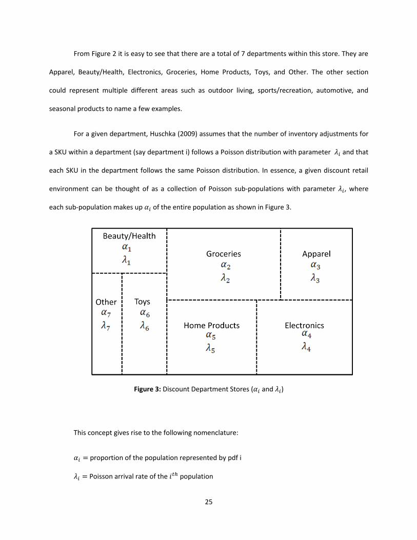
From Figure 2 it is easy to see that there are a total of 7 departments within this store. They are
Apparel, Beauty/Health, Electronics, Groceries, Home Products, Toys, and Other. The other section
could represent multiple different areas such as outdoor living, sports/recreation, automotive, and
seasonal products to name a few examples.
For a given department, Huschka (2009) assumes that the number of inventory adjustments for
a SKU within a department (say department i) follows a Poisson distribution with parameter and that
each SKU in the department follows the same Poisson distribution. In essence, a given discount retail
environment can be thought of as a collection of Poisson sub-populations with parameter , where
each sub-population makes up of the entire population as shown in Figure 3.
Figure 3: Discount Department Stores ( and )
This concept gives rise to the following nomenclature:
proportion of the population represented by pdf i
Poisson arrival rate of the population
26
number of SKU’s sampled to assess inventory adjustments for the population
number of sub-populations
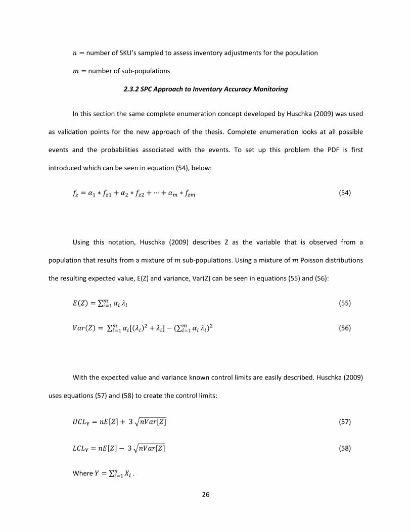
2.3.2 SPC Approach to Inventory Accuracy Monitoring
In this section the same complete enumeration concept developed by Huschka (2009) was used
as validation points for the new approach of the thesis. Complete enumeration looks at all possible
events and the probabilities associated with the events. To set up this problem the PDF is first
introduced which can be seen in equation (54), below:
(54)
Using this notation, Huschka (2009) describes Z as the variable that is observed from a
population that results from a mixture of sub-populations. Using a mixture of Poisson distributions
the resulting expected value, E(Z) and variance, Var(Z) can be seen in equations (55) and (56):
(55)
(56)
With the expected value and variance known control limits are easily described. Huschka (2009)
uses equations (57) and (58) to create the control limits:
(57)
(58)
Where .
27
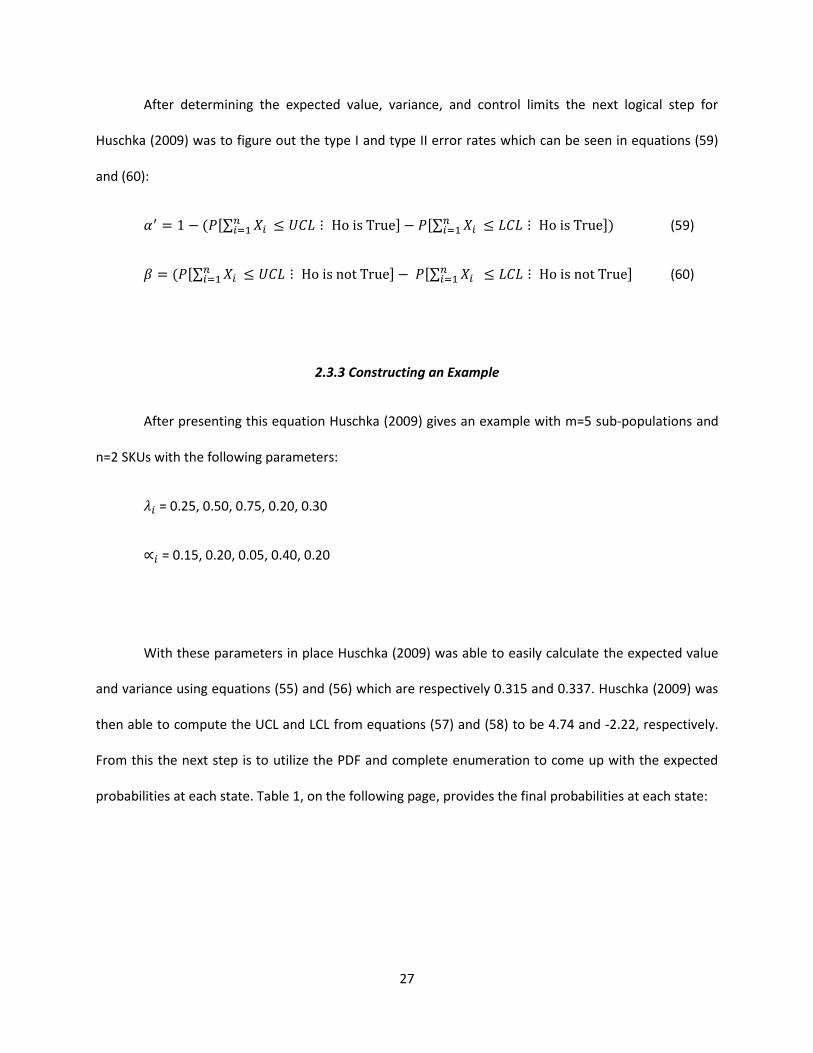
After determining the expected value, variance, and control limits the next logical step for
Huschka (2009) was to figure out the type I and type II error rates which can be seen in equations (59)
and (60):
(59)
(60)
2.3.3 Constructing an Example
After presenting this equation Huschka (2009) gives an example with m=5 sub-populations and
n=2 SKUs with the following parameters:
= 0.25, 0.50, 0.75, 0.20, 0.30
= 0.15, 0.20, 0.05, 0.40, 0.20
With these parameters in place Huschka (2009) was able to easily calculate the expected value
and variance using equations (55) and (56) which are respectively 0.315 and 0.337. Huschka (2009) was
then able to compute the UCL and LCL from equations (57) and (58) to be 4.74 and -2.22, respectively.
From this the next step is to utilize the PDF and complete enumeration to come up with the expected
probabilities at each state. Table 1, on the following page, provides the final probabilities at each state:

28
Table 1: Complete Enumeration Example
Y= X1 + X2 Prob(Y)
0 0.54375953
1 0.32079783
2 0.104350788
3 0.025076815
4 0.004989009
5 0.000867797
6 0.000135831
7 1.94586E-05
8 2.58001E-06
9 3.19167E-07
10 3.7063E-08
11 4.0588E-09
Sum 0.999999999
From Table 1, it is seen that once at 11 errors the sum of the probabilities is close enough to 1 to
stop calculating past this point. With the cumulative probabilities in place the next step is to calculate
the type I error rate by utilizing the calculated UCL, LCL, and equation (59), which turns out to be
.001026.
29
Chapter 3: Defining Sub-populations of SKUs
This chapter provides analysis of data from a national leader in retail. Due to time constraints
and the large amount of data that were received, only the electronics department was used for analysis.
All of the work that is done with the electronics department could easily be reapplied to the other
departments within this retail environment.
3.1 Defining Sub-Populations
Before analysis on the data could be performed there needed to be defined sub-populations
with SKU’s in each sub-population that were a good fit. To do this, SKUs were broken into logical
categories that were believed to follow similar distributions. For example a 46” TV is assumed to follow
a similar pattern as a 32” TV, therefore, these two would be grouped together. Once logical groups were
assigned, Minitab software was utilized to complete the statistical analysis to see if every combination
of SKUs within the sub-population followed a similar distribution. To do this, a two sample t-test was run
for each SKU within the population against every other SKU within the population. A 95% confidence
interval was examined for the difference between these SKUs. The equations that were used to perform
the two sample t-test can be seen below in formulas (61), (62), and (63):
(61)
(62)
(63)
30
In these equations, Y represents the number of errors found within the SKU while n represents
the total number of observations for each SKU. If “0” was found to be within the confidence interval
then it was determined for the purposes of this research that these two SKU’s were similar enough to be
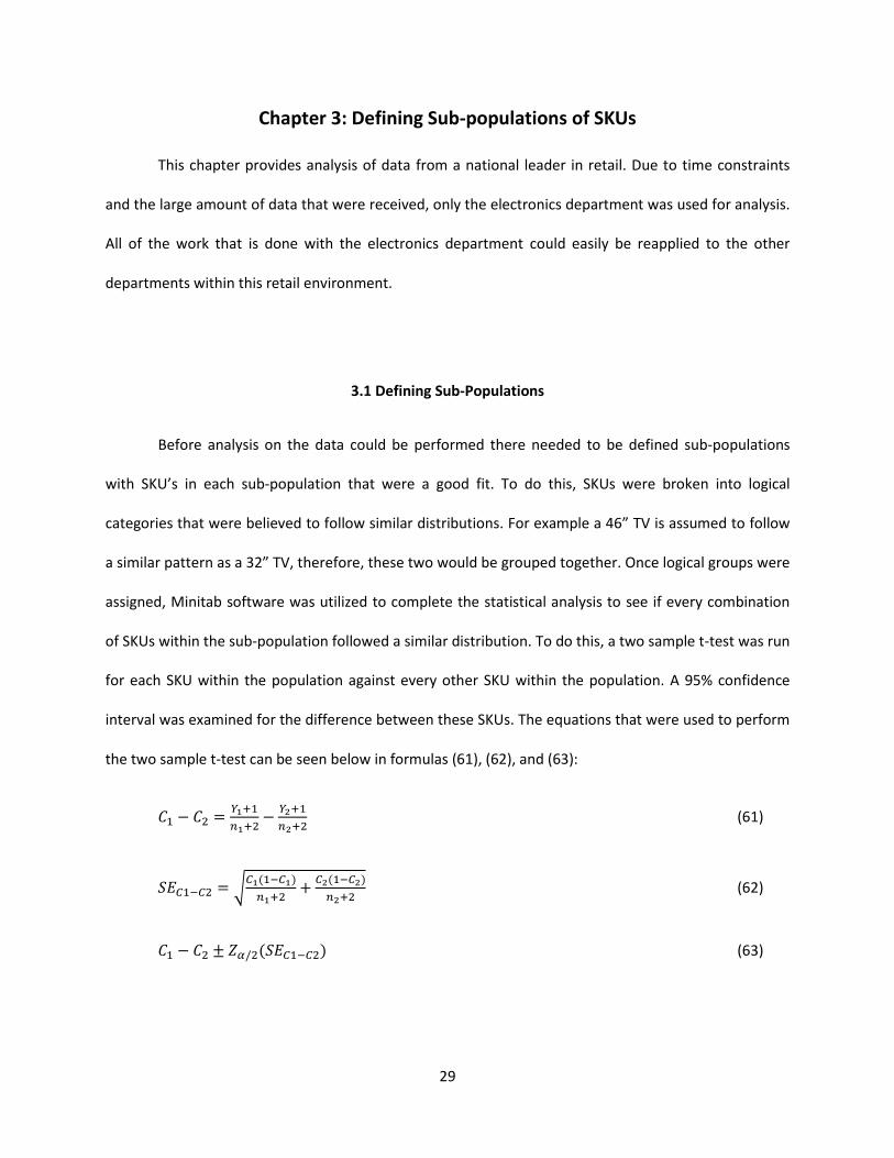
in the same sub-population. For each sub-population that was looked at, a data matrix was completed
to show the confidence interval of each SKU with every other SKU within the sub-population. An
example of one of these matrixes can be seen below in Figure 4.
Figure 4: Home Electronics t-test Matrix
Figure 4 shows that every SKU within this sub-population has a similar mean. Five additional
sub-populations were similarly considered. In each case, games, home electronics, accessories,
computer, ink, and TV/DVD, similar mean characteristics were found for those sub-populations;
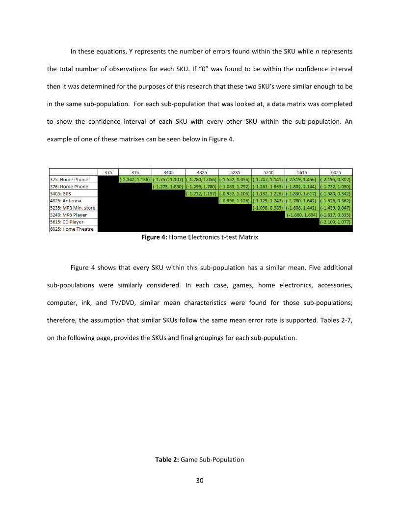
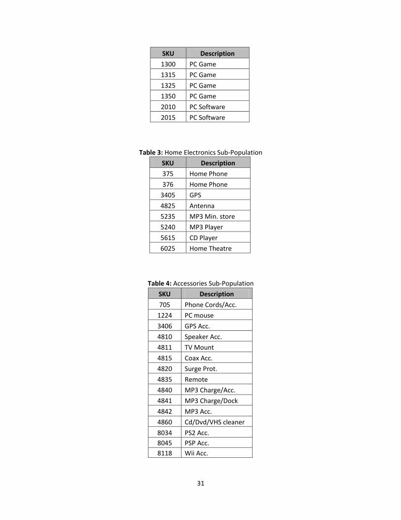
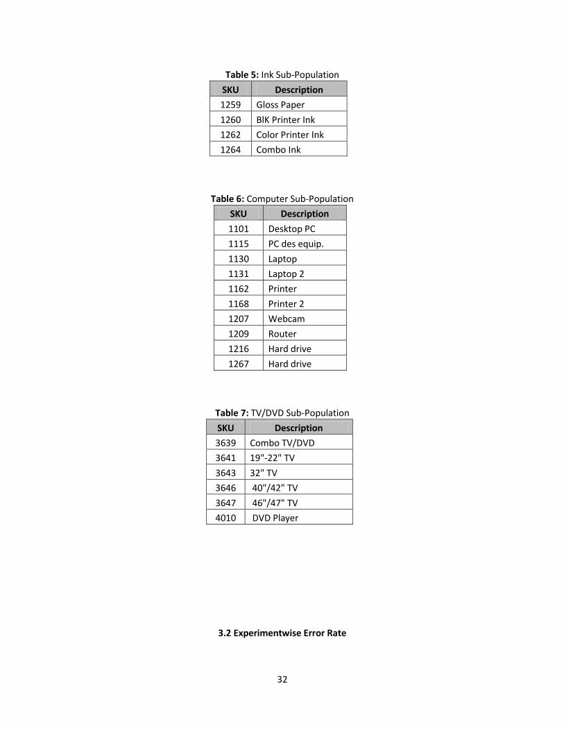
therefore, the assumption that similar SKUs follow the same mean error rate is supported. Tables 2-7,
on the following page, provides the SKUs and final groupings for each sub-population.
Table 2: Game Sub-Population
31
SKU Description
1300 PC Game
1315 PC Game
1325 PC Game
1350 PC Game
2010 PC Software
2015 PC Software
Table 3: Home Electronics Sub-Population
SKU Description
375 Home Phone
376 Home Phone
3405 GPS
4825 Antenna
5235 MP3 Min. store
5240 MP3 Player
5615 CD Player
6025 Home Theatre
Table 4: Accessories Sub-Population
SKU Description
705 Phone Cords/Acc.
1224 PC mouse
3406 GPS Acc.
4810 Speaker Acc.
4811 TV Mount
4815 Coax Acc.
4820 Surge Prot.
4835 Remote
4840 MP3 Charge/Acc.
4841 MP3 Charge/Dock
4842 MP3 Acc.
4860 Cd/Dvd/VHS cleaner
8034 PS2 Acc.
8045 PSP Acc.
8118 Wii Acc.
32
Table 5: Ink Sub-Population
SKU Description
1259 Gloss Paper
1260 BlK Printer Ink
1262 Color Printer Ink
1264 Combo Ink
Table 6: Computer Sub-Population
SKU Description
1101 Desktop PC
1115 PC des equip.
1130 Laptop
1131 Laptop 2
1162 Printer
1168 Printer 2
1207 Webcam
1209 Router
1216 Hard drive
1267 Hard drive
Table 7: TV/DVD Sub-Population
SKU Description
3639 Combo TV/DVD
3641 19"-22" TV
3643 32" TV
3646 40"/42" TV
3647 46"/47" TV
4010 DVD Player
3.2 Experimentwise Error Rate
33
It is important to note that the experimentwise error rate is likely very large for our pragmatic
approach within this chapter. The values for all the experiments considered is greater than the
individual experiment. Steel and Torrie (1980) state that a true experimentwise error rate must clearly
allow any and all possible hypotheses to be tested and that it is desired that each treatment has a
meaningful set of contrasts. The experimentwise error rate approximation can be seen in equation (64),
below:
(64)
is the experimentwise error rate, is the per comparison error rate, and C is the number
of comparisons. In the case of the home electronics scenario the per comparison error rate was set at
.05 and there were a total of 28 comparisons made. In this case the experimentwise error rate would be
.7622. This is high and it is likely that there is at least one type I error, but we believe there is
overwhelming evidence of similar mean characteristics. With our research it is understood that there is
a good chance of inflated type I errors due to the procedures we used to make sub-populations. It is
important to be conscious of this as results are examined later in the research.

34
Chapter 4: Computer Program
Small values of n have been examined for the SPC approach to cycle counting in Huschka (2009)
using complete enumeration. In this chapter, we present a recursive approach to consider larger sample
sizes. This approach is embedded in a computer program so that larger sample sizes can be considered.
The data that was provided by the large retail environment was utilized to compare the results of the
program with the results of complete enumeration. We will show that this program can achieve the
same type I error rates as complete enumeration for n=1, n=2, and n=3. After n=3 complete
enumeration becomes quite computationally burdensome.
4.1 Defining the Recursive Relationship
As stated previously, complete enumeration becomes computationally burdensome and is not
effective to utilize as n grows larger. Miller (2008) develops an approach called conditional probabilities
that is further used by Huschka (2009). Although this method is somewhat effective for estimating type I
error rates, it is not effective for large sample sizes. With a recursive relationship, loops can easily be set
to calculate n for much larger sizes, to provide precise estimates of type I error rates. Equations (65),
(66), and (67) show the relationship that was developed:
(65)
(66)
(67)

35
From equation (65), (66), and (67) the nomenclature follows as n is the total number of SKUs, i is
the total number of errors, and j is the current iteration of the errors. Equation (65) initializes the
recursive function. Q gives the final probability at n=1 for each error, j. Using this initialization it is
possible to utilize this equation to solve for any value of n as seen in equation (66). The final equation
(67) determines the final type I error. With this recursive equation in place it is easy to examine larger
sizes of n. The next step was developing a program that could read data and take the necessary steps to
find error rates for the data.
4.2 Computer Program
A computer program was created to calculate larger values of n and can be found in Appendix A.
There are two main parts to the program. The first part begins reading the number of product types in
each sub-population and the corresponding and values. Once these values are calculated, the
program utilizes equations (54) and (55) to find the expected value and variance for the sub-population.
With the expected value and variance the LCL and UCL can be calculated with equations (56) and (57).
The second part of the program applies the recursive relationship to calculate each of the probabilities
and ultimately find the type I error rate. The final program takes the and values that are specified by
the user and give a print out from n=1 to n=150. This can be edited to be larger or smaller depending on
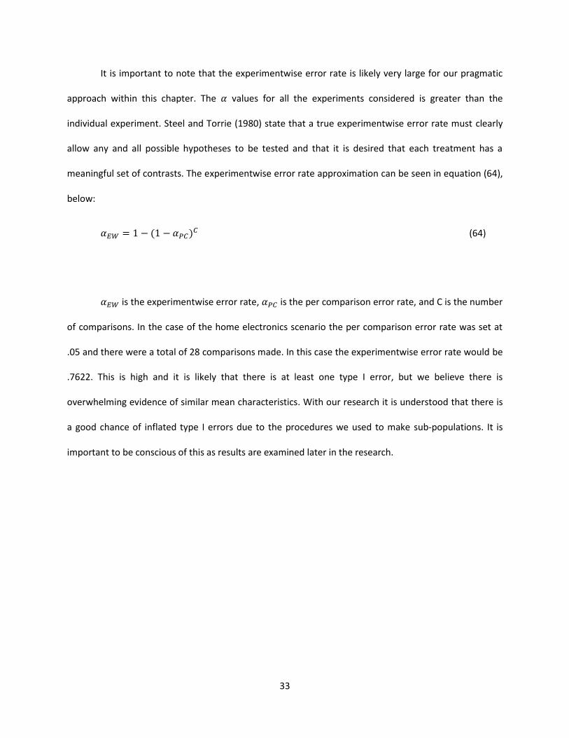
preference of the user. Figure 5, below, is an example of the output screen from the program.
36
Figure 5: Computer Program Output
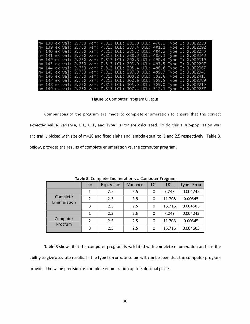
Comparisons of the program are made to complete enumeration to ensure that the correct
expected value, variance, LCL, UCL, and Type I error are calculated. To do this a sub-population was
arbitrarily picked with size of m=10 and fixed alpha and lambda equal to .1 and 2.5 respectively. Table 8,
below, provides the results of complete enumeration vs. the computer program.
Table 8: Complete Enumeration vs. Computer Program
n= Exp. Value Variance LCL UCL Type I Error
Complete Enumeration
1 2.5 2.5 0 7.243 0.004245
2 2.5 2.5 0 11.708 0.00545
3 2.5 2.5 0 15.716 0.004603
Computer Program
1 2.5 2.5 0 7.243 0.004245
2 2.5 2.5 0 11.708 0.00545
3 2.5 2.5 0 15.716 0.004603
Table 8 shows that the computer program is validated with complete enumeration and has the
ability to give accurate results. In the type I error rate column, it can be seen that the computer program
provides the same precision as complete enumeration up to 6 decimal places.

37
Chapter 5: Type I Error Rates
Based upon observations made analyzing real world data, an experiment of numerous different
type I error rates are constructed to evaluate the type I error rate in a balanced fashion. There are
numerous different type I error rates that could be examined, but ultimately the real world retail
environment data is used to derive the type I error rates examined. In this section larger values of n and
differing sub-populations are examined. Specifically, n=5, n=75, and n=150 are explored. Additionally
m=5, m=10, and m=15 are examined. Defining the and values that are utilized is a little more
complex and will be explained in the following section.
5.1 Defining and Values
In this section we will explore and values when m=5, but any of the scenarios can be
replicated for differing values of m. Five different methods are used for which are fixed, delta
increase, delta decrease, skewed top, and skewed bottom. When observing values it is important to
keep in mind that each value is a proportion of the population and thus the sum of all the ’s within a
sub-population must add up to 1. When the values are fixed the total proportion of the sub-
population, 1, is divided by the size of the sub-population, m. This can be seen in equation (68):
(68)
In the fixed scenario when observing m=5, =.2 for all ’s within the sub-population. The next
scenario for is delta increase and delta decrease. These two states are calculated in the same manner
the only difference is increase starts at the minimum and goes to the maximum, while decrease starts at
the maximum and goes to the minimum. The initialization of this state can be seen, below, in equation
(69):
(69)
38
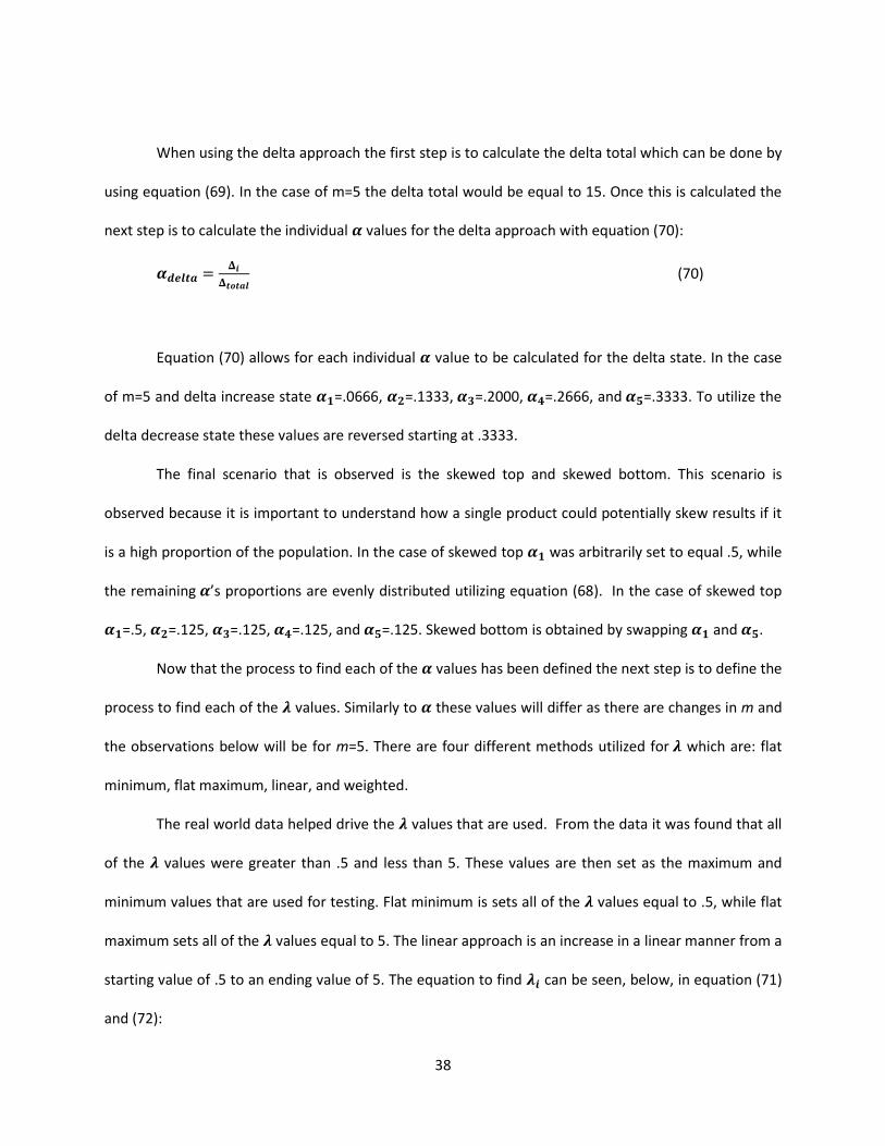
When using the delta approach the first step is to calculate the delta total which can be done by
using equation (69). In the case of m=5 the delta total would be equal to 15. Once this is calculated the
next step is to calculate the individual values for the delta approach with equation (70):
(70)
Equation (70) allows for each individual value to be calculated for the delta state. In the case
of m=5 and delta increase state =.0666, =.1333, =.2000, =.2666, and =.3333. To utilize the
delta decrease state these values are reversed starting at .3333.
The final scenario that is observed is the skewed top and skewed bottom. This scenario is
observed because it is important to understand how a single product could potentially skew results if it
is a high proportion of the population. In the case of skewed top was arbitrarily set to equal .5, while
the remaining ’s proportions are evenly distributed utilizing equation (68). In the case of skewed top
=.5, =.125, =.125, =.125, and =.125. Skewed bottom is obtained by swapping and .
Now that the process to find each of the values has been defined the next step is to define the
process to find each of the values. Similarly to these values will differ as there are changes in m and
the observations below will be for m=5. There are four different methods utilized for which are: flat
minimum, flat maximum, linear, and weighted.
The real world data helped drive the values that are used. From the data it was found that all
of the values were greater than .5 and less than 5. These values are then set as the maximum and
minimum values that are used for testing. Flat minimum is sets all of the values equal to .5, while flat
maximum sets all of the values equal to 5. The linear approach is an increase in a linear manner from a
starting value of .5 to an ending value of 5. The equation to find can be seen, below, in equation (71)
and (72):
39
(71)
(72)
In equation (71) 4.5 is used because it is the difference between 5 and .5. When looking at m=5
the values are as follows = .5, = 1.625, =2 .75, = 3.875, and = 5. The final approach for
values is the weighted scenario. This is similar to the idea of skewed ’s. All of the values are at the
minimum of .5 while the last value in the sub-population is heavily weighted with a value of 5. Each of
the approaches outlined in this section is chose to test numerous different possible scenarios that could
occur in the real world. It is not an exhaustive list of possible scenarios that can happen in the real
world. The exact values that are used in each of these different scenarios are found in Appendix B.
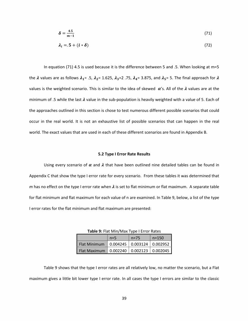
5.2 Type I Error Rate Results
Using every scenario of and that have been outlined nine detailed tables can be found in
Appendix C that show the type I error rate for every scenario. From these tables it was determined that
m has no effect on the type I error rate when is set to flat minimum or flat maximum. A separate table
for flat minimum and flat maximum for each value of n are examined. In Table 9, below, a list of the type
I error rates for the flat minimum and flat maximum are presented:
Table 9: Flat Min/Max Type I Error Rates
n=5 n=75 n=150
Flat Minimum 0.004245 0.003124 0.002952
Flat Maximum 0.002240 0.002123 0.002045
Table 9 shows that the type I error rates are all relatively low, no matter the scenario, but a Flat
maximum gives a little bit lower type I error rate. In all cases the type I errors are similar to the classic
40
chart with normality assumed, but it does appear that the SPC approach may have a bit better type I
error for larger or average inventory inaccuracy.
It is also important to note that as n increases the type I error rate continues to decrease. We
now extend our type I error rates to conditions of linear and weighted. Table 10, below, has the type I
error rates for the linear and weighted scenarios:
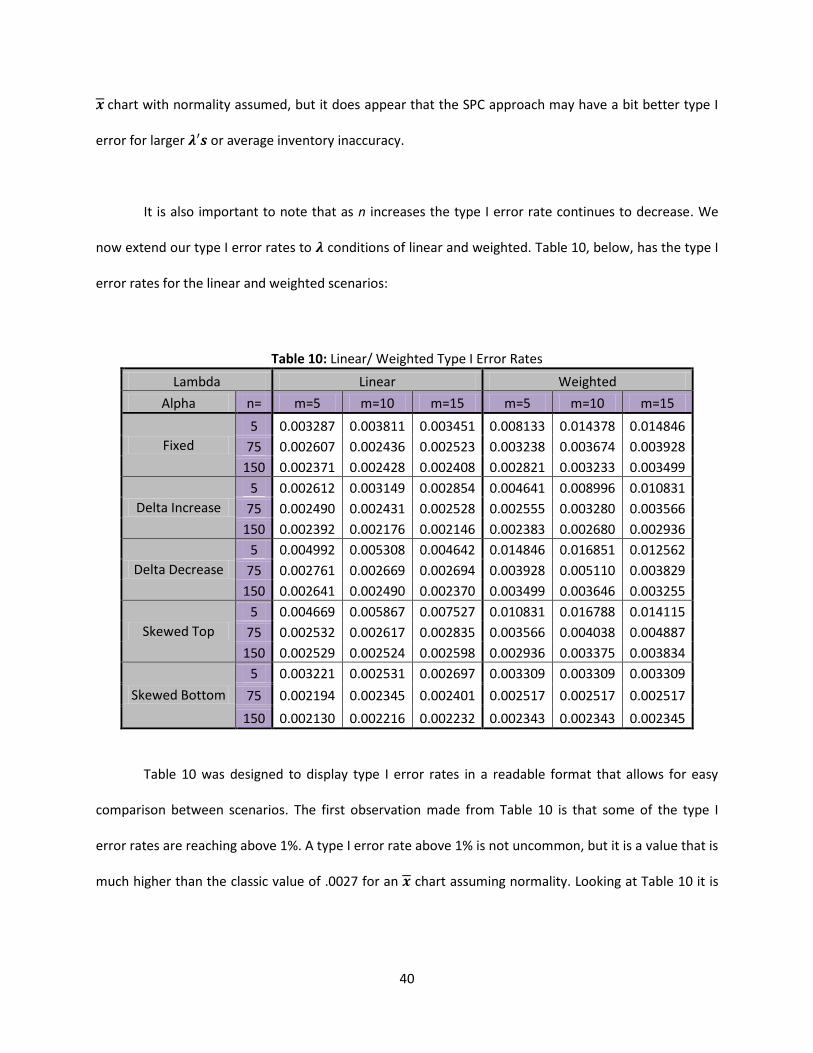
Table 10: Linear/ Weighted Type I Error Rates
Lambda Linear Weighted
Alpha n= m=5 m=10 m=15 m=5 m=10 m=15
Fixed
5 0.003287 0.003811 0.003451 0.008133 0.014378 0.014846
75 0.002607 0.002436 0.002523 0.003238 0.003674 0.003928
150 0.002371 0.002428 0.002408 0.002821 0.003233 0.003499
Delta Increase
5 0.002612 0.003149 0.002854 0.004641 0.008996 0.010831
75 0.002490 0.002431 0.002528 0.002555 0.003280 0.003566
150 0.002392 0.002176 0.002146 0.002383 0.002680 0.002936
Delta Decrease
5 0.004992 0.005308 0.004642 0.014846 0.016851 0.012562
75 0.002761 0.002669 0.002694 0.003928 0.005110 0.003829
150 0.002641 0.002490 0.002370 0.003499 0.003646 0.003255
Skewed Top
5 0.004669 0.005867 0.007527 0.010831 0.016788 0.014115
75 0.002532 0.002617 0.002835 0.003566 0.004038 0.004887
150 0.002529 0.002524 0.002598 0.002936 0.003375 0.003834
Skewed Bottom
5 0.003221 0.002531 0.002697 0.003309 0.003309 0.003309
75 0.002194 0.002345 0.002401 0.002517 0.002517 0.002517
150 0.002130 0.002216 0.002232 0.002343 0.002343 0.002345
Table 10 was designed to display type I error rates in a readable format that allows for easy
comparison between scenarios. The first observation made from Table 10 is that some of the type I
error rates are reaching above 1%. A type I error rate above 1% is not uncommon, but it is a value that is
much higher than the classic value of .0027 for an chart assuming normality. Looking at Table 10 it is

41
noted that all of the values above 1% occurred when is weighted and n=5. There is some evidence that
increasing n for the weighted conditions of may lead to excessive type I error rates.
In the weighted scenario, all of the values are set to .5 except for a single value that is set to 5.
This causes a high variance for the number of errors and pushes the control limits further out. When
looking at lower values of n, the calculation of the LCL will return a negative value that is outside the
realm of feasible errors. In the case of UCL, it does not get out far enough to make up for the large
variance in probabilities, and in turn, it causes the type I error rate to increase. From looking at Table 10
it is seen that the type I error rate is well below 1% when n=75 or n=150. This should not be a cause for
a concern.
The second finding from Table 10 is that type I error rates decrease as n increases. This is no
surprise, as such behavior is expected due to the central limit theorem. Table 10 confirms the
hypothesis and matches the findings from Table 9. When n=150 it is evident that the highest type I error
rate is .003834. As with Table 9 this is not below the .0027 that is necessary to meet the normality
assumption, but is still an acceptable type I error rate.
5.3 Type I Error Rate Conclusions
Several general observations are made from Table 9 and Table 10. The first was that no matter
what value of m, if the are equal, the type I error rate is the same for all conditions. This makes
logical sense because the expected value and variance are the same no matter how many sub-
populations exist.
The second observation made is that as n increases the type I error rate dwindles. As this is
examined further it is found that this is what should be expected. The central limit theorem states that
as sample sizes increase, with a mean and variance, the sampling distribution of the mean approaches a

42
normal distribution. In our scenarios, the sampling distribution is tending to a normal distribution as
more SKUs are pulled from the mixture Poisson process. This is the cause for slight decrease in the the
type I error rates as n increases.
The final observation made is that the majority of our type I error rates were below 1% which is
an acceptable level. However, there are a few cases in which the type I error rate is seen to inflate
higher than 1%. The only cases of this happening were when n=5 with set to weighted. It is
determined that this is due to the large variance that is caused when is weighted. From these findings
it can be determined that this would not be a serious issue for any real world environment because it is
unlikely that a real world retail environment would ever be looking at such small values of n. It is
however important to note this and keep it in mind when looking at scenarios that would come close to
fitting a weighted state.

43
Chapter 6: Type II Error Rates
In this section type II error rates are discussed. Shifts in at 10%, 25%, and 35% will be
observed. Since type I error rates are calculated for nine different tables above with three different
shifts in this would require a total of 27 tables. The same table format will be utilized as was used for
type I error rates. Appendix D presents all 27 tables and these may be referenced as necessary. Before
moving forward it is important to mention that this is not an exhaustive list of all type II error rates. In
fact there are an infinite number of scenarios for which type II error rates could be determined. This
section provides a balanced set of scenarios and examines how different shifts in affect the type II
error rates.
6.1 Type II Error Rates Shift
A smaller shift of begin the examination of type II error rates. This is determined to be
small by running numerous tests and finding that the type II error rates were unlikely to be detected in
most scenarios. In Table 11, below, the type II error rates for flat minimum and flat maximum can be
seen at different levels of n:
Table 11: Flat Min/Max, Type II Error Rates
n=5 n=75 n=150
Flat Minimum 0.999411 0.997919 0.993811
Flat Maximum 0.998703 0.908302 0.727124
When n=5, both flat minimum and flat maximum have fairly high type II error rates which means
it is unlikely that this shift would be detected. As n starts to increase it is observed that the type II error
rate decreases for both flat minimum and flat maximum. When looking at flat maximum, it is seen that it

44
decreases at a much faster rate as n increases, since the flat maximum has much higher values of than
flat minimum. If a higher is shifted by a percentage it causes the shifted ’s to increase at a faster rate.
As the values of increase, the expected value will also increase. Thus a shift with higher values will
cause its expected value to move away from the assumed expected value of the control limits at a much
faster rate. This allows for quicker detection of a type II error rate, because it more quickly moves away
from the mean as the shift increases. In Table 12, below, we present the type II errors for linear and
weighted ’s with a 10% increase:
Table 12: Linear/ Weighted, Type II Error Rates
Lambda Linear Weighted
Alpha n= m=5 m=10 m=15 m=5 m=10 m=15
Fixed
5 0.998952 0.998764 0.998900 0.995902 0.994410 0.994102
75 0.988917 0.988462 0.987505 0.998757 0.999220 0.999060
150 0.968217 0.961694 0.963686 0.996467 0.997809 0.998351
Delta Increase
5 0.999246 0.993420 0.999100 0.998124 0.996924 0.993901
75 0.977045 0.975535 0.973590 0.997302 0.998816 0.999081
150 0.931200 0.917313 0.913742 0.992634 0.996698 0.997459
Delta Decrease
5 0.997988 0.998796 0.998175 0.994102 0.988564 0.991189
75 0.994695 0.993649 0.993119 0.998757 0.998964 0.998233
150 0.983399 0.980218 0.976875 0.998351 0.997903 0.996157
Skewed Top
5 0.998079 0.997430 0.997910 0.993901 0.993295 0.998599
75 0.996231 0.996960 0.996786 0.999081 0.999104 0.990800
150 0.989766 0.990549 0.990625 0.997495 0.998354 0.990109
Skewed Bottom
5 0.999497 0.999329 0.999589 0.999365 0.999365 0.999365
75 0.981053 0.976383 0.973948 0.993985 0.993985 0.993984
150 0.942092 0.929416 0.924577 0.983733 0.983733 0.983732
Similar to Table 11, we see that in Table 12 the type II error rates are relatively high. This should
not be of any concern because it is a small shift in . Similar to the type I error rate, the type II
error rate decreases as n increases in almost every scenario examined in Table 12.
45
It should be noted there are some cases that when n increases there is not a decrease in the
type II error rate. These cases were isolated only to the scenario when is in the weighted state. These
few rare cases are examined and it is found that it only occurred when moving from n=5 to n=75. It is
observed that there are ten cases where it didn’t decrease and of these cases the largest increase was
by .010004.
This is a similar situation to the problems observed with the weighted state for type I error
rates. Due to the high variance of the values, the distribution becomes quite dispersed. In the case of
n=5, the type II error rate is lower because the LCL is truncated to zero, and the UCL is unable to detect
the dispersion. This is not a huge concern, but is important to note when looking at data similar to the
weighted state at low levels of n. There could also be some round off error due to the utilization of a
program, but the values are small enough it is not of any concern. A larger shift in is explored in the
next section.
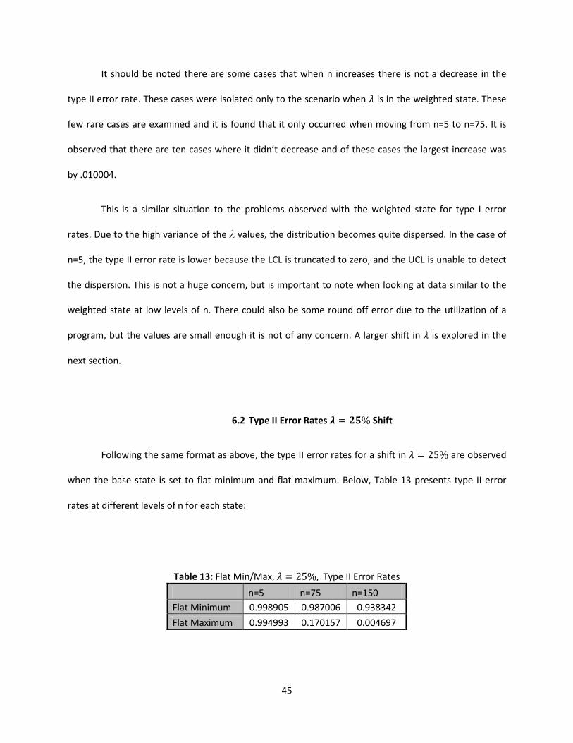
6.2 Type II Error Rates Shift
Following the same format as above, the type II error rates for a shift in are observed
when the base state is set to flat minimum and flat maximum. Below, Table 13 presents type II error
rates at different levels of n for each state:
Table 13: Flat Min/Max, Type II Error Rates
n=5 n=75 n=150
Flat Minimum 0.998905 0.987006 0.938342
Flat Maximum 0.994993 0.170157 0.004697
46
Table 13 meets all the conditions that were observed in Table 11. It can be seen that the type II
error rate decrease as n increases and that flat maximum is decreasing at a much faster rate than flat
minimum. It is somewhat alarming to see n=150 return one type II error rate equal to .938342 and
another equal to .004697. After further investigation, it can be attributed to the larger values
compared to such small values. Keep in mind that two extremes for values are used when looking at
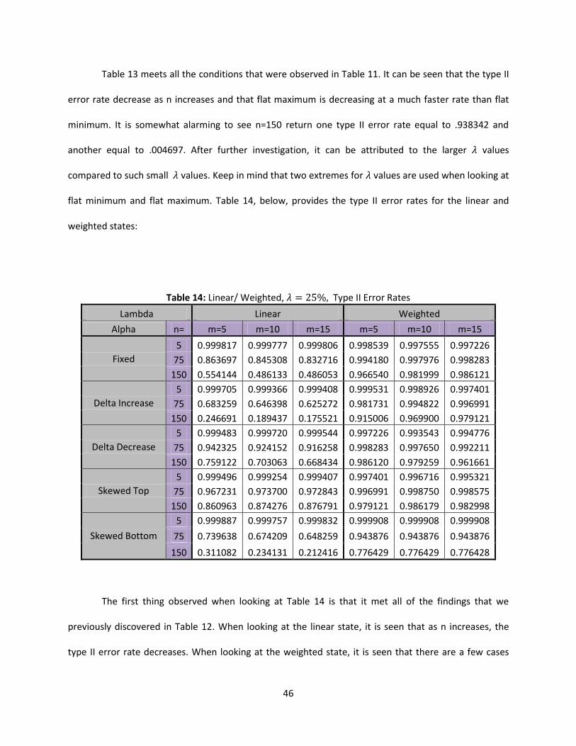
flat minimum and flat maximum. Table 14, below, provides the type II error rates for the linear and
weighted states:
Table 14: Linear/ Weighted, Type II Error Rates
Lambda Linear Weighted
Alpha n= m=5 m=10 m=15 m=5 m=10 m=15
Fixed
5 0.999817 0.999777 0.999806 0.998539 0.997555 0.997226
75 0.863697 0.845308 0.832716 0.994180 0.997976 0.998283
150 0.554144 0.486133 0.486053 0.966540 0.981999 0.986121
Delta Increase
5 0.999705 0.999366 0.999408 0.999531 0.998926 0.997401
75 0.683259 0.646398 0.625272 0.981731 0.994822 0.996991
150 0.246691 0.189437 0.175521 0.915006 0.969900 0.979121
Delta Decrease
5 0.999483 0.999720 0.999544 0.997226 0.993543 0.994776
75 0.942325 0.924152 0.916258 0.998283 0.997650 0.992211
150 0.759122 0.703063 0.668434 0.986120 0.979259 0.961661
Skewed Top
5 0.999496 0.999254 0.999407 0.997401 0.996716 0.995321
75 0.967231 0.973700 0.972843 0.996991 0.998750 0.998575
150 0.860963 0.874276 0.876791 0.979121 0.986179 0.982998
Skewed Bottom
5 0.999887 0.999757 0.999832 0.999908 0.999908 0.999908
75 0.739638 0.674209 0.648259 0.943876 0.943876 0.943876
150 0.311082 0.234131 0.212416 0.776429 0.776429 0.776428
The first thing observed when looking at Table 14 is that it met all of the findings that we
previously discovered in Table 12. When looking at the linear state, it is seen that as n increases, the
type II error rate decreases. When looking at the weighted state, it is seen that there are a few cases

47
that the type II error rates are not decreasing as n is increasing. In Table 14 there were only six cases of
the type II error rate not decreasing as n increased. Like Table 12, it only happened from n=5 to n=75. It
was also found that the largest discrepancy between the two values was an increase of .004017 which is
much better than .010004 we saw in Table 12. It is seen that potential round off errors have lessened in
table 8.
When is shifted it moves the entire distribution to the right which allows for improved
detection. This is important with a highly variable state with a low level of n because the control limits
are now detecting more probabilities within the realm of possible errors. As shifts in continue to grow
this issue will dwindle until reaching a point that the type II error rates will all decrease as any value of n
increases.
The final observation that was made from Table 14 is that Type II error rates drop in many of the
scenarios. It was observed that the cases that type II error rates reached prevalent levels were when
n=150, and it was set to a linear state. There was also somewhat of a trend when was equal to skewed
bottom and delta increase. In these cases there were larger drops in the type II error rate. These findings
will continue to be monitored as larger shifts in are explored.
6.3 Type II Error Rates Shift
The final shift in a type II Error rate that will be observed will be a shift in . Below, Table
15 shows the type II error rates with a base condition set to flat minimum and flat maximum:
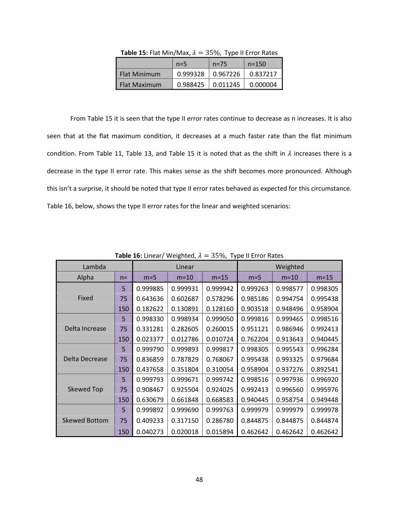
48
Table 15: Flat Min/Max, Type II Error Rates
n=5 n=75 n=150
Flat Minimum 0.999328 0.967226 0.837217
Flat Maximum 0.988425 0.011245 0.000004
From Table 15 it is seen that the type II error rates continue to decrease as n increases. It is also
seen that at the flat maximum condition, it decreases at a much faster rate than the flat minimum
condition. From Table 11, Table 13, and Table 15 it is noted that as the shift in increases there is a
decrease in the type II error rate. This makes sense as the shift becomes more pronounced. Although
this isn’t a surprise, it should be noted that type II error rates behaved as expected for this circumstance.
Table 16, below, shows the type II error rates for the linear and weighted scenarios:
Table 16: Linear/ Weighted, Type II Error Rates
Lambda Linear Weighted
Alpha n= m=5 m=10 m=15 m=5 m=10 m=15
Fixed
5 0.999885 0.999931 0.999942 0.999263 0.998577 0.998305
75 0.643636 0.602687 0.578296 0.985186 0.994754 0.995438
150 0.182622 0.130891 0.128160 0.903518 0.948496 0.958904
Delta Increase
5 0.998330 0.998934 0.999050 0.999816 0.999465 0.998516
75 0.331281 0.282605 0.260015 0.951121 0.986946 0.992413
150 0.023377 0.012786 0.010724 0.762204 0.913643 0.940445
Delta Decrease
5 0.999790 0.999893 0.999817 0.998305 0.995543 0.996284
75 0.836859 0.787829 0.768067 0.995438 0.993325 0.979684
150 0.437658 0.351804 0.310054 0.958904 0.937276 0.892541
Skewed Top
5 0.999793 0.999671 0.999742 0.998516 0.997936 0.996920
75 0.908467 0.925504 0.924025 0.992413 0.996560 0.995976
150 0.630679 0.661848 0.668583 0.940445 0.958754 0.949448
Skewed Bottom
5 0.999892 0.999690 0.999763 0.999979 0.999979 0.999978
75 0.409233 0.317150 0.286780 0.844875 0.844875 0.844874
150 0.040273 0.020018 0.015894 0.462642 0.462642 0.462642

49
When studying Table 16 the first finding noted is that there is evidence that supported a
previous theory. From Table 14 it was hypothesized that as shifts in increased there would be a point
at which all type II error rates would decrease as any value of n increases. When looking at Table 16
every case that n increases results in a decrease in .
The second observation is that there are definitive trends that are causing type II error rates to
drop. The first of these trends that is observed is that in almost every case when comparing a type II
error rate with constant , m, and n the linear state will result in a lower type II error rate than the
weighted state. The only time this did not happen was in a few cases when n=5. This is due to the high
variability with a low value of n that was previously discussed.
There are two causes for the lower type II error rates for the linear state. The first is because it
has lower variability like the weighted state. This means that the control limits are much tighter and as
shifts occur they will move out of the control limits faster and allow them to be detected more quickly.
The second reason is that the linear state has much higher values of than in the weighted state. These
values are higher ’s causing the expected value to change much quicker thus moving away from the
assumed mean quicker.
The next trend that was seen was that when was set to delta increase and skewed bottom,
detection of type II error rates happened quicker. This relates back to having ’s that are at a higher
level thus causing a higher expected value. In the case of the delta increase and skewed bottom the
highest proportioned value lines up with the highest value of . This causes the expected value to be
much higher than other scenarios and causes shifts to move away from the mean at a much quicker
rate. The conclusion section ties all of these findings together.
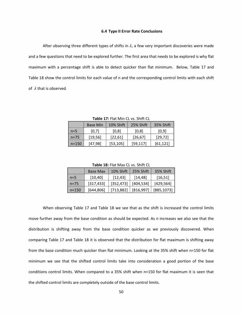
50
6.4 Type II Error Rate Conclusions
After observing three different types of shifts in , a few very important discoveries were made
and a few questions that need to be explored further. The first area that needs to be explored is why flat
maximum with a percentage shift is able to detect quicker than flat minimum. Below, Table 17 and
Table 18 show the control limits for each value of n and the corresponding control limits with each shift
of that is observed.
Table 17: Flat Min CL vs. Shift CL
Base Min 10% Shift 25% Shift 35% Shift
n=5 [0,7] [0,8] [0,8] [0,9]
n=75 [19,56] [22,61] [26,67] [29,72]
n=150 [47,98] [53,105] [59,117] [61,121]
When observing Table 17 and Table 18 we see that as the shift is increased the control limits
move further away from the base condition as should be expected. As n increases we also see that the
distribution is shifting away from the base condition quicker as we previously discovered. When
comparing Table 17 and Table 18 it is observed that the distribution for flat maximum is shifting away
from the base condition much quicker than flat minimum. Looking at the 35% shift when n=150 for flat
minimum we see that the shifted control limits take into consideration a good portion of the base
conditions control limits. When compared to a 35% shift when n=150 for flat maximum it is seen that
the shifted control limits are completely outside of the base control limits.
Table 18: Flat Max CL vs. Shift CL
Base Max 10% Shift 25% Shift 35% Shift
n=5 [10,40] [12,43] [14,48] [16,51]
n=75 [317,433] [352,473] [404,534] [429,564]
n=150 [644,806] [713,882] [816,997] [885,1073]

51
This is the reason that in this scenario we see a type II error rate of .837217 for flat minimum
while flat maximum returns a type II error rate of .000004. When observing percentage shifts the flat
maximum will move quicker out of the base conditions control limits due to a higher expected value.
This makes it much easier to detect shifts when values are higher or there is significant weight put on
an individual value.
Another important take away from the type II error rate analysis was that m has minimal effect
on the resulting type II error rate. Through all of the tables when everything else was held constant
comparing type II error rates for different values of m gave very similar results. There was only one
instance when there was a discrepancy larger than .06 in all of the tables. The majority of
inconsistencies happened when using values that had repeating decimals which caused numerical
instability.
The third finding from the type II error rate examination was that when there is a single value
that is highly weighted it causes a high variance. Due to this high variance the probabilities stretch out
and this causes an issue for small values of n. In the case of n=5 this causes the type II error rate to be
lower because the LCL pushes negative and the UCL is unable to detect the large variance of
probabilities.
The final conclusion from the type II error rate analysis is that as n increases a decrease in the
type II error rate can be expected. Although this can’t be assumed for every state it is definitely the case
in a large majority of the scenarios. The only time this conclusion was not valid was when was set to
the weighted state for the reasons listed in the previous paragraph. It is important that when
performing analysis on data to keep this in mind and understand how to find a scenario that would
resemble the weighted state.

52
Chapter 7: Conclusion and Future Work
7.1 Conclusions
The work by Huschka (2009) set the background for this thesis and brought up the need to
examine larger sample sizes. Huschka proposed simulation, but we developed a recursive approach that
eliminated the need for simulation. The development of this thesis has successfully advanced the belief
that SPC can be utilized as an efficient method to improve inventory control systems in a real world
environment as Huschka (2009) believed to be the case. Although complete enumeration was an
effective method to find type I error rates for small values of n, it was impossible to apply this to real
world environments for large sample sizes. The development of a recursive function and a program that
can calculate large values of n proved that SPC is utilized in a resourceful and practical manner. There
are a few important lessons and findings from this research that will now briefly be discussed.
As n increases a decrease in type I and type II error rates should be expected in most scenarios.
It was found that the only time this did not occur is when looking at smaller values of n and when is set
to the weighted state. To avoid these issues it would be recommended to observe your values closely
to ensure that there is not a single value that is an outlier from the rest of the sub-population. It is also
suggested that when utilizing the SPC approach to use sample sizes greater than 50.
This research was able to determine that m has minimal to no affect on type I and type II error
rates. It was found that there was some variance due to round off error and repeating decimals, but it
was negligible in most scenarios. This is an important find because it allows the practitioner to make
comparisons between sub-populations of different sizes of m.

53
The final finding from this research was the effect larger expected values have on the detection
rate of type II errors. When observing percentage shifts, the flat maximum distribution will move quicker
out of the base conditions control limits due to a higher expected value. This will assist the practitioner
when observing the expected values of differing populations and making connections to the type II error
rates. In the future work section we will look at a method that allows for equal detection of type II error
rates and other methods to advance this research.
7.1 Future Work
The research completed in this thesis takes the previous work of Huschka (2009) and proves the
usefulness of SPC in real world retail environments. With this progression, the next steps of this work
should be to look at methods to further improve upon the current model and computer program work
that was created in this thesis.
The modeling techniques used in this thesis only scratched the surface of possible situations
that could come up in the real world. Type II errors could be extended beyond just the shifts in that
are observed in this research. Model shifts in should be examined first. Additionally, since an
analytical approach is now available for large sample sizes the type I error rates should be fixed at .0027.
Then from there finding the resulting type II error rates could be analyzed. This would allow for an equal
detection process for all type II error rates.
Aside from the modeling techniques, there are also significant improvements that need to be
made to the computer program. In its current state, it is effective for finding type I and type II error
rates, but it is not efficient. For each value in the type II error rate table , m, n, and control limits
had to be adjusted manually. After entering each of these values, the program calculates the type II

54
error rate for that specific location in the table. Adding on to the program to allow it to calculate type II
error rates for different values of m and n for a certain set of and values would allow it to be much
more efficient. There are also memory allocation issues. The current program can only calculate up to
values of n=150. After that point issues start to occur and the program crashes. It would be a huge
improvement to rework resource allocations within the program to allow it to calculate up to n=200.
The final area to progress the work in this thesis is to utilize an updated and efficient computer
program to observe a retail environment over a period of time. Although real world data was used in
this thesis, it was a snapshot of data. Being able to observe data over a six month to one year period
would allow for the observation of the complexities of a real world environment over time. This could
open up new ideas on how to improve the current work and show that the current work is effective in
all situations instead of isolated scenarios.
55
References
Brooks, R., & Wilson, L. (2005). Inventory Record Accuracy - Unleashing the Power of Cycle Counting.
Atlanta: John-Wiley & Sons.
Burroughs, T.E., Rigdon, S.E., and Champ, C.W. (1993). “An Analysis of Shewhart Charts with
Run Rules When No Standards Are Given,” Proceedings of the Quality and Productivity
Section of the American Statistical Association, August 8-12, San Francisco, CA, pp. 16-
19.
Calzada, M. E., & Scariano, S. M. (2003). Reconciling the integral equation and Markov chain approaches
for computing EWMA average run lengths. Communications in Statistics Part B: Simulation and
Computation, 32(2), 591-604.
Castagliola, P. (2005). A R-EWMA control chart for monitoring the process range. International Journal of
Reliability, Quality and Safety Engineering, 12(1), 31-49.
Champ, C.W., and Woodall, W.H. (1987). “Exact Results for Shewhart Control Charts with
Supplementary Runs Rules,” Technometrics, Vol. 29, No. 4, pp. 393-399.
Costa, A. F., & Magalhaes, M. D. (2007). An adaptive chart for monitoring the process mean and
variance. Quality and Reliability Engineering International, 23(7), 821-831.
Cozzucoli, P. (2009). Process Monitoring with Multivariate p-Control Chart. International Journal of
Quality, Statistics and Reliability, 9, 11-18.
Crowder, S. (1987). A Simple Method for Studying Run-Length Distributions of Exponentially Weighted
Moving Average Charts. Technometrics, 29(4), 401-407.
Dehoratius, N., & Raman, A. (2008). Inventory record inaccuracy: An empirical analysis. Management
Science, 54(4), 627-641.
Gan, F. (1993). An Optimal Design of CUSUM Control Charts for Binomial Counts. Journal of Applied

56
Statistics, 20(4), 172-183.
Huschka, K (2009). Using Staistical Process Control to Monitor Inventory Accuracy. Proceedings of the
2010 Material Handling Colloqium, June 2010. Milwaukee, WI. CD-ROM
Khoo, M. (2004). Poisson moving average versus c chart for nonconformities. Quality Engineering, 16(4),
525-534.
Kok, G. A., & Shang, K. H. (2007). Inspection and replenishment policies for systems with inventory
record inaccuracy. Manufacturing and Service Operations Management, 9(2), 185-205.
Lapinski, K., & Dessouky, M. (1994). Optimal selection of sampling locations and c-chart parameters.
Computers and Industrial Engineering, 27(1), 297-300.
Montgomery, D. (2009). Introduction to Statistical Quality Control, 5th Ed.. New York : John-Wiley &
Sons.
Marcellus, R. (2008). Bayesian Monitoring to detect a shift in process mean. Quality and Reliability
Engineering International, 24(3), 303-313.
Ou, Y., Jiao, J., & Wu, Z. (2009). Control charts applications for multivariate attribute processes. IEEE
International Conference on Industrial Engineering and Engineering Management, 1, 408-413.
Piasecki, D. (2003). Inventory Accuracy: People, Processes, and Technology. Kenosha, WI: Ops Publishing.
Rossetti, M., Collins, T., & Kurgund, R. (2001). Inventory Cycle Counting - A Review. The proceedings of
the 2001 Industrial Engineering Research Conference, 1, 457-463.
Rudisill, F., Litteral, L., & Walter, D. (2004). Modified U charts for monitoring and controlling poisson
attribute processes. Quality Engineering, 16(4), 637-642.
Schreibfeder, J. (n.d.). Cycle Counting Can Eliminate Your Annual Physical Inventory! (Part 1). Effective
Inventory Management. Retrieved November 8, 2010, from
http://www.effectiveinventory.com/article9.html
Shewhart, W. (1926). Quality Control Charts. Bell Systems Technical Journal, 1, 593-603.

57
Shewhart, W. (1927). Quality Control Charts. Bell Systems Technical Journal, 2, 722-735.
Spliid, H. (2010). An exponentially weighted moving average control chart for Bernoulli data. Quality and
Reliability Engineering International, 26(1), 97-113.
Taleb, H. (2009). Control charts applications for multivariate attribute processes. Computers and
Industrial Engineering, , 56(1), 399-410.
Steel, R. and Torrie, J. (1980). Principles and Procedures of Statistics, Second Edition, New York: McGraw-
Hill.
Wang, C., Dong, T., & Way, K. (2009). A hybrid approach for identification of concurrent control chart
patterns. Journal of Intelligent Manufacturing, 20(4), 409-419.
Woodall, W. (1997). Control Charts Based on Attribute Data: Bibliography and Review. Journal of Quality
Technology , 29(2), 172-183.
Yu, L. (2007). A Statistical Process Control Approach to Cycle Counting for Retail Environments.

58
Appendix A – Computer Program
#include "stdafx.h" #include <stdio.h> #include <stdlib.h> #include <time.h> #include "math.h" typedef struct Data_S Data; typedef struct Families_S Families; typedef struct Product_S Product; #define MAXFAMILY 1 #define MAXITER 151 #define MAXSKUS 16 #define MAXHISTORY 0 #define MAXERRORS 822 struct Data_S { Families *family; int numfamilies; int totaldatapts; double *totalerrorprob; }; struct Families_S { Product *prod; int numprod; double ucl[MAXITER]; double lcl[MAXITER]; double expectval; double var; double prob[MAXITER][MAXERRORS]; }; struct Product_S { double alpha; double lamda; double *probabilities; int probabilitylength; int *errorhistory; int historylength; int familynum;
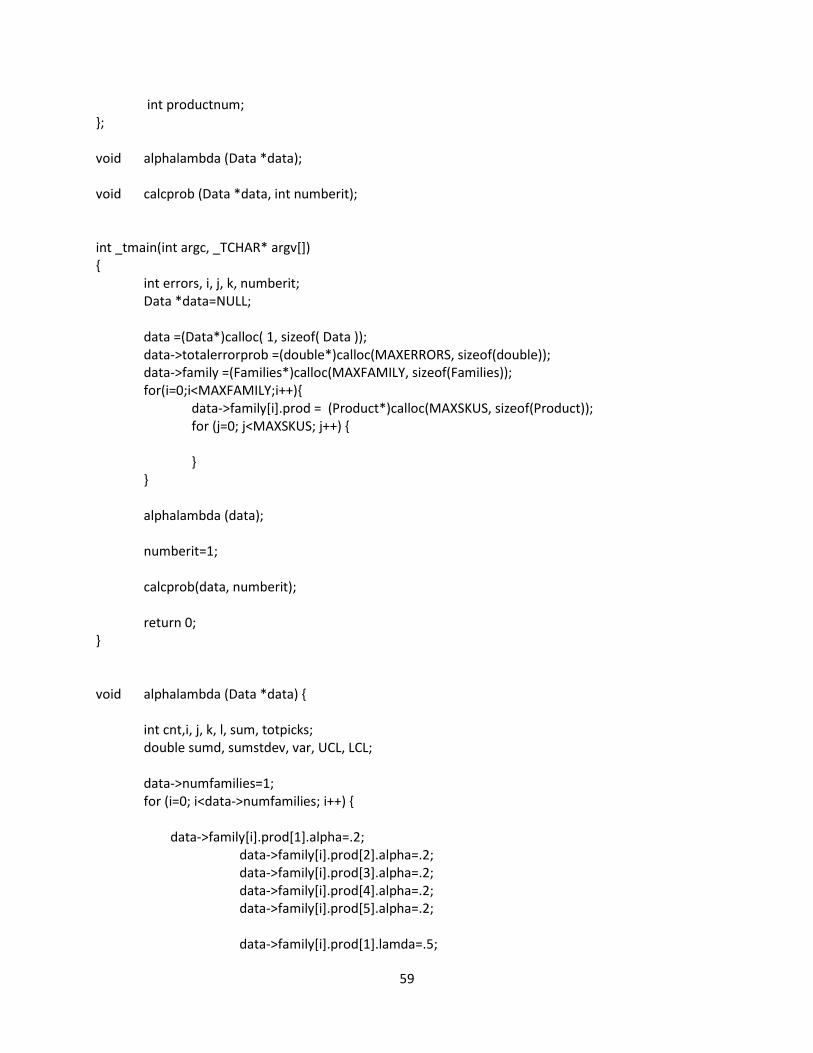
59
int productnum; }; void alphalambda (Data *data); void calcprob (Data *data, int numberit); int _tmain(int argc, _TCHAR* argv[]) { int errors, i, j, k, numberit; Data *data=NULL; data =(Data*)calloc( 1, sizeof( Data )); data->totalerrorprob =(double*)calloc(MAXERRORS, sizeof(double)); data->family =(Families*)calloc(MAXFAMILY, sizeof(Families)); for(i=0;i<MAXFAMILY;i++){ data->family[i].prod = (Product*)calloc(MAXSKUS, sizeof(Product)); for (j=0; j<MAXSKUS; j++) { } } alphalambda (data); numberit=1; calcprob(data, numberit); return 0; } void alphalambda (Data *data) { int cnt,i, j, k, l, sum, totpicks; double sumd, sumstdev, var, UCL, LCL; data->numfamilies=1; for (i=0; i<data->numfamilies; i++) { data->family[i].prod[1].alpha=.2; data->family[i].prod[2].alpha=.2; data->family[i].prod[3].alpha=.2; data->family[i].prod[4].alpha=.2; data->family[i].prod[5].alpha=.2; data->family[i].prod[1].lamda=.5;

60
data->family[i].prod[2].lamda=.5; data->family[i].prod[3].lamda=.5; data->family[i].prod[4].lamda=.5; data->family[i].prod[5].lamda=.5; data->family[i].numprod=5; } getchar(); for (i=0; i<data->numfamilies; i++) { sumd=0; for (j=1; j<=data->family[i].numprod; j++) { } } for (i=0; i<data->numfamilies; i++) { sumd=0; sumstdev=0; for (j=1; j<=data->family[i].numprod; j++) { sumd+=data->family[i].prod[j].alpha*data->family[i].prod[j].lamda; sumstdev+=data->family[i].prod[j].alpha*(((data->family[i].prod[j].lamda*data->family[i].prod[j].lamda)+data->family[i].prod[j].lamda)); var=sumstdev-(sumd*sumd); } data->family[i].var=var; data->family[i].expectval=sumd; for (j=1; j<MAXITER; j++) { data->family[i].lcl[j]=(double)j*data->family[i].expectval-3*sqrt(j*data->family[i].var); data->family[i].ucl[j]=(double)j*data->family[i].expectval+3*sqrt(j*data->family[i].var); if ( data->family[i].lcl[j]<0) data->family[i].lcl[j]=0; } } } void calcprob (Data *data, int numberit) { int cnt,i, j, k, l, m, totpicks;
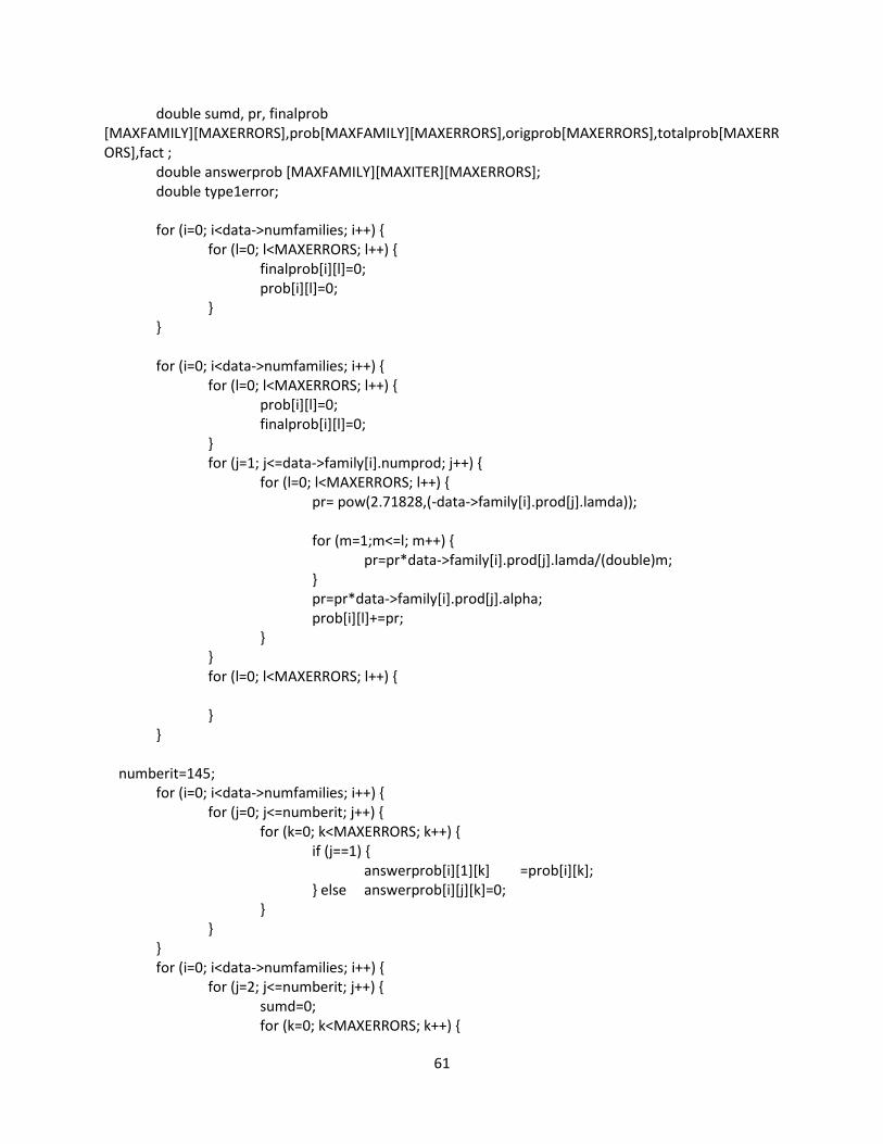
61
double sumd, pr, finalprob [MAXFAMILY][MAXERRORS],prob[MAXFAMILY][MAXERRORS],origprob[MAXERRORS],totalprob[MAXERRORS],fact ; double answerprob [MAXFAMILY][MAXITER][MAXERRORS]; double type1error; for (i=0; i<data->numfamilies; i++) { for (l=0; l<MAXERRORS; l++) { finalprob[i][l]=0; prob[i][l]=0; } } for (i=0; i<data->numfamilies; i++) { for (l=0; l<MAXERRORS; l++) { prob[i][l]=0; finalprob[i][l]=0; } for (j=1; j<=data->family[i].numprod; j++) { for (l=0; l<MAXERRORS; l++) { pr= pow(2.71828,(-data->family[i].prod[j].lamda)); for (m=1;m<=l; m++) { pr=pr*data->family[i].prod[j].lamda/(double)m; } pr=pr*data->family[i].prod[j].alpha; prob[i][l]+=pr; } } for (l=0; l<MAXERRORS; l++) { } } numberit=145; for (i=0; i<data->numfamilies; i++) { for (j=0; j<=numberit; j++) { for (k=0; k<MAXERRORS; k++) { if (j==1) { answerprob[i][1][k] =prob[i][k]; } else answerprob[i][j][k]=0; } } } for (i=0; i<data->numfamilies; i++) { for (j=2; j<=numberit; j++) { sumd=0; for (k=0; k<MAXERRORS; k++) {
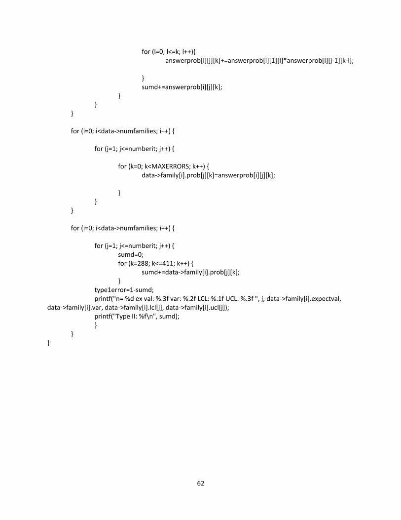
62
for (l=0; l<=k; l++){ answerprob[i][j][k]+=answerprob[i][1][l]*answerprob[i][j-1][k-l]; } sumd+=answerprob[i][j][k]; } } } for (i=0; i<data->numfamilies; i++) { for (j=1; j<=numberit; j++) { for (k=0; k<MAXERRORS; k++) { data->family[i].prob[j][k]=answerprob[i][j][k]; } } } for (i=0; i<data->numfamilies; i++) { for (j=1; j<=numberit; j++) { sumd=0; for (k=288; k<=411; k++) { sumd+=data->family[i].prob[j][k]; } type1error=1-sumd; printf("n= %d ex val: %.3f var: %.2f LCL: %.1f UCL: %.3f ", j, data->family[i].expectval, data->family[i].var, data->family[i].lcl[j], data->family[i].ucl[j]); printf("Type II: %f\n", sumd); } } }
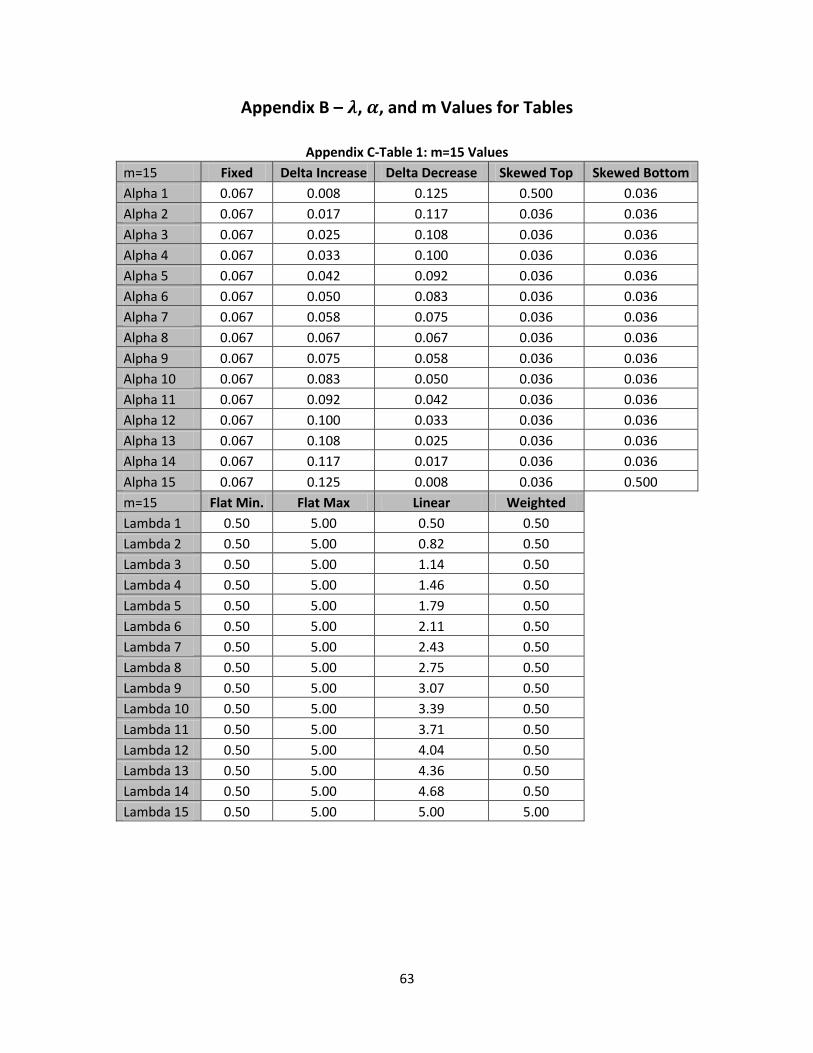
63
Appendix B – , , and m Values for Tables
Appendix C-Table 1: m=15 Values
m=15 Fixed Delta Increase Delta Decrease Skewed Top Skewed Bottom
Alpha 1 0.067 0.008 0.125 0.500 0.036
Alpha 2 0.067 0.017 0.117 0.036 0.036
Alpha 3 0.067 0.025 0.108 0.036 0.036
Alpha 4 0.067 0.033 0.100 0.036 0.036
Alpha 5 0.067 0.042 0.092 0.036 0.036
Alpha 6 0.067 0.050 0.083 0.036 0.036
Alpha 7 0.067 0.058 0.075 0.036 0.036
Alpha 8 0.067 0.067 0.067 0.036 0.036
Alpha 9 0.067 0.075 0.058 0.036 0.036
Alpha 10 0.067 0.083 0.050 0.036 0.036
Alpha 11 0.067 0.092 0.042 0.036 0.036
Alpha 12 0.067 0.100 0.033 0.036 0.036
Alpha 13 0.067 0.108 0.025 0.036 0.036
Alpha 14 0.067 0.117 0.017 0.036 0.036
Alpha 15 0.067 0.125 0.008 0.036 0.500
m=15 Flat Min. Flat Max Linear Weighted Lambda 1 0.50 5.00 0.50 0.50 Lambda 2 0.50 5.00 0.82 0.50 Lambda 3 0.50 5.00 1.14 0.50 Lambda 4 0.50 5.00 1.46 0.50 Lambda 5 0.50 5.00 1.79 0.50 Lambda 6 0.50 5.00 2.11 0.50 Lambda 7 0.50 5.00 2.43 0.50 Lambda 8 0.50 5.00 2.75 0.50 Lambda 9 0.50 5.00 3.07 0.50 Lambda 10 0.50 5.00 3.39 0.50 Lambda 11 0.50 5.00 3.71 0.50 Lambda 12 0.50 5.00 4.04 0.50 Lambda 13 0.50 5.00 4.36 0.50 Lambda 14 0.50 5.00 4.68 0.50 Lambda 15 0.50 5.00 5.00 5.00
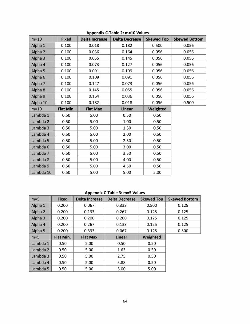
64
Appendix C-Table 2: m=10 Values
m=10 Fixed Delta Increase Delta Decrease Skewed Top Skewed Bottom
Alpha 1 0.100 0.018 0.182 0.500 0.056
Alpha 2 0.100 0.036 0.164 0.056 0.056
Alpha 3 0.100 0.055 0.145 0.056 0.056
Alpha 4 0.100 0.073 0.127 0.056 0.056
Alpha 5 0.100 0.091 0.109 0.056 0.056
Alpha 6 0.100 0.109 0.091 0.056 0.056
Alpha 7 0.100 0.127 0.073 0.056 0.056
Alpha 8 0.100 0.145 0.055 0.056 0.056
Alpha 9 0.100 0.164 0.036 0.056 0.056
Alpha 10 0.100 0.182 0.018 0.056 0.500
m=10 Flat Min. Flat Max Linear Weighted Lambda 1 0.50 5.00 0.50 0.50 Lambda 2 0.50 5.00 1.00 0.50 Lambda 3 0.50 5.00 1.50 0.50 Lambda 4 0.50 5.00 2.00 0.50 Lambda 5 0.50 5.00 2.50 0.50 Lambda 6 0.50 5.00 3.00 0.50 Lambda 7 0.50 5.00 3.50 0.50 Lambda 8 0.50 5.00 4.00 0.50 Lambda 9 0.50 5.00 4.50 0.50 Lambda 10 0.50 5.00 5.00 5.00
Appendix C-Table 3: m=5 Values
m=5 Fixed Delta Increase Delta Decrease Skewed Top Skewed Bottom
Alpha 1 0.200 0.067 0.333 0.500 0.125
Alpha 2 0.200 0.133 0.267 0.125 0.125
Alpha 3 0.200 0.200 0.200 0.125 0.125
Alpha 4 0.200 0.267 0.133 0.125 0.125
Alpha 5 0.200 0.333 0.067 0.125 0.500
m=5 Flat Min. Flat Max Linear Weighted Lambda 1 0.50 5.00 0.50 0.50 Lambda 2 0.50 5.00 1.63 0.50 Lambda 3 0.50 5.00 2.75 0.50 Lambda 4 0.50 5.00 3.88 0.50 Lambda 5 0.50 5.00 5.00 5.00
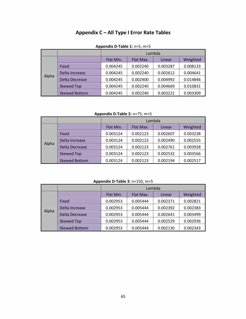
65
Appendix C – All Type I Error Rate Tables
Appendix D-Table 1: n=5, m=5
Lambda
Alpha
Flat Min. Flat Max. Linear Weighted
Fixed 0.004245 0.002240 0.003287 0.008133
Delta Increase 0.004245 0.002240 0.002612 0.004641
Delta Decrease 0.004245 0.002400 0.004992 0.014846
Skewed Top 0.004245 0.002240 0.004669 0.010831
Skewed Bottom 0.004245 0.002240 0.003221 0.003309
Appendix D-Table 2: n=75, m=5
Lambda
Alpha
Flat Min. Flat Max. Linear Weighted
Fixed 0.003124 0.002123 0.002607 0.003238
Delta Increase 0.003124 0.002123 0.002490 0.002555
Delta Decrease 0.003124 0.002123 0.002761 0.003928
Skewed Top 0.003124 0.002123 0.002532 0.003566
Skewed Bottom 0.003124 0.002123 0.002194 0.002517
Appendix D-Table 3: n=150, m=5
Lambda
Alpha
Flat Min. Flat Max. Linear Weighted
Fixed 0.002953 0.005444 0.002371 0.002821
Delta Increase 0.002953 0.005444 0.002392 0.002383
Delta Decrease 0.002953 0.005444 0.002641 0.003499
Skewed Top 0.002953 0.005444 0.002529 0.002936
Skewed Bottom 0.002953 0.005444 0.002130 0.002343
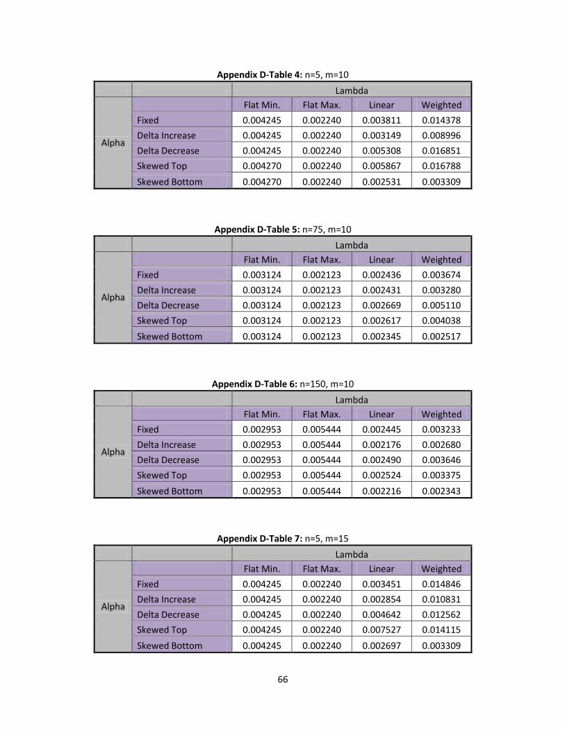
66
Appendix D-Table 4: n=5, m=10
Lambda
Alpha
Flat Min. Flat Max. Linear Weighted
Fixed 0.004245 0.002240 0.003811 0.014378
Delta Increase 0.004245 0.002240 0.003149 0.008996
Delta Decrease 0.004245 0.002240 0.005308 0.016851
Skewed Top 0.004270 0.002240 0.005867 0.016788
Skewed Bottom 0.004270 0.002240 0.002531 0.003309
Appendix D-Table 5: n=75, m=10
Lambda
Alpha
Flat Min. Flat Max. Linear Weighted
Fixed 0.003124 0.002123 0.002436 0.003674
Delta Increase 0.003124 0.002123 0.002431 0.003280
Delta Decrease 0.003124 0.002123 0.002669 0.005110
Skewed Top 0.003124 0.002123 0.002617 0.004038
Skewed Bottom 0.003124 0.002123 0.002345 0.002517
Appendix D-Table 6: n=150, m=10
Lambda
Alpha
Flat Min. Flat Max. Linear Weighted
Fixed 0.002953 0.005444 0.002445 0.003233
Delta Increase 0.002953 0.005444 0.002176 0.002680
Delta Decrease 0.002953 0.005444 0.002490 0.003646
Skewed Top 0.002953 0.005444 0.002524 0.003375
Skewed Bottom 0.002953 0.005444 0.002216 0.002343
Appendix D-Table 7: n=5, m=15
Lambda
Alpha
Flat Min. Flat Max. Linear Weighted
Fixed 0.004245 0.002240 0.003451 0.014846
Delta Increase 0.004245 0.002240 0.002854 0.010831
Delta Decrease 0.004245 0.002240 0.004642 0.012562
Skewed Top 0.004245 0.002240 0.007527 0.014115
Skewed Bottom 0.004245 0.002240 0.002697 0.003309
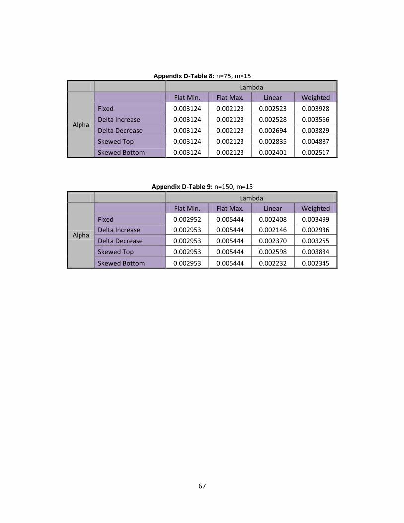
67
Appendix D-Table 8: n=75, m=15
Lambda
Alpha
Flat Min. Flat Max. Linear Weighted
Fixed 0.003124 0.002123 0.002523 0.003928
Delta Increase 0.003124 0.002123 0.002528 0.003566
Delta Decrease 0.003124 0.002123 0.002694 0.003829
Skewed Top 0.003124 0.002123 0.002835 0.004887
Skewed Bottom 0.003124 0.002123 0.002401 0.002517
Appendix D-Table 9: n=150, m=15
Lambda
Alpha
Flat Min. Flat Max. Linear Weighted
Fixed 0.002952 0.005444 0.002408 0.003499
Delta Increase 0.002953 0.005444 0.002146 0.002936
Delta Decrease 0.002953 0.005444 0.002370 0.003255
Skewed Top 0.002953 0.005444 0.002598 0.003834
Skewed Bottom 0.002953 0.005444 0.002232 0.002345
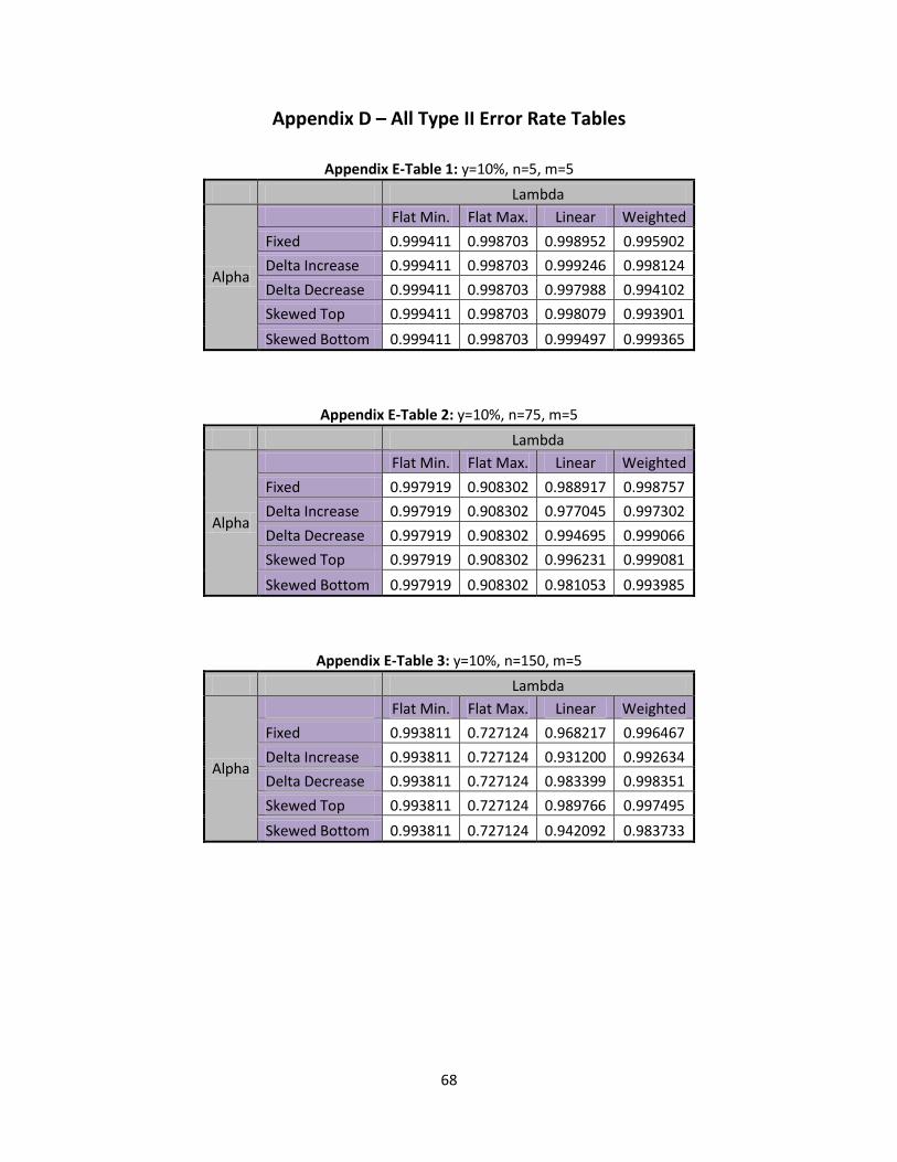
68
Appendix D – All Type II Error Rate Tables
Appendix E-Table 1: y=10%, n=5, m=5
Lambda
Alpha
Flat Min. Flat Max. Linear Weighted
Fixed 0.999411 0.998703 0.998952 0.995902
Delta Increase 0.999411 0.998703 0.999246 0.998124
Delta Decrease 0.999411 0.998703 0.997988 0.994102
Skewed Top 0.999411 0.998703 0.998079 0.993901
Skewed Bottom 0.999411 0.998703 0.999497 0.999365
Appendix E-Table 2: y=10%, n=75, m=5
Lambda
Alpha
Flat Min. Flat Max. Linear Weighted
Fixed 0.997919 0.908302 0.988917 0.998757
Delta Increase 0.997919 0.908302 0.977045 0.997302
Delta Decrease 0.997919 0.908302 0.994695 0.999066
Skewed Top 0.997919 0.908302 0.996231 0.999081
Skewed Bottom 0.997919 0.908302 0.981053 0.993985
Appendix E-Table 3: y=10%, n=150, m=5
Lambda
Alpha
Flat Min. Flat Max. Linear Weighted
Fixed 0.993811 0.727124 0.968217 0.996467
Delta Increase 0.993811 0.727124 0.931200 0.992634
Delta Decrease 0.993811 0.727124 0.983399 0.998351
Skewed Top 0.993811 0.727124 0.989766 0.997495
Skewed Bottom 0.993811 0.727124 0.942092 0.983733
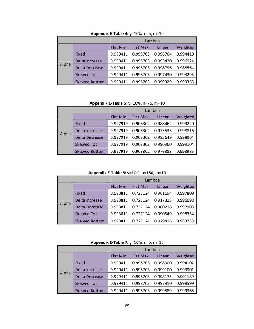
69
Appendix E-Table 4: y=10%, n=5, m=10
Lambda
Alpha
Flat Min. Flat Max. Linear Weighted
Fixed 0.999411 0.998703 0.998764 0.994410
Delta Increase 0.999411 0.998703 0.993420 0.996924
Delta Decrease 0.999411 0.998703 0.998796 0.988564
Skewed Top 0.999411 0.998703 0.997430 0.993295
Skewed Bottom 0.999411 0.998703 0.999329 0.999365
Appendix E-Table 5: y=10%, n=75, m=10
Lambda
Alpha
Flat Min. Flat Max. Linear Weighted
Fixed 0.997919 0.908302 0.988462 0.999220
Delta Increase 0.997919 0.908302 0.975535 0.998816
Delta Decrease 0.997919 0.908302 0.993649 0.998964
Skewed Top 0.997919 0.908302 0.996960 0.999104
Skewed Bottom 0.997919 0.908302 0.976383 0.993985
Appendix E-Table 6: y=10%, n=150, m=10
Lambda
Alpha
Flat Min. Flat Max. Linear Weighted
Fixed 0.993811 0.727124 0.961694 0.997809
Delta Increase 0.993811 0.727124 0.917313 0.996698
Delta Decrease 0.993811 0.727124 0.980218 0.997903
Skewed Top 0.993811 0.727124 0.990549 0.998354
Skewed Bottom 0.993811 0.727124 0.929416 0.983733
Appendix E-Table 7: y=10%, n=5, m=15
Lambda
Alpha
Flat Min. Flat Max. Linear Weighted
Fixed 0.999411 0.998703 0.998900 0.994102
Delta Increase 0.999411 0.998703 0.999100 0.993901
Delta Decrease 0.999411 0.998703 0.998175 0.991189
Skewed Top 0.999411 0.998703 0.997910 0.998599
Skewed Bottom 0.999411 0.998703 0.999589 0.999365
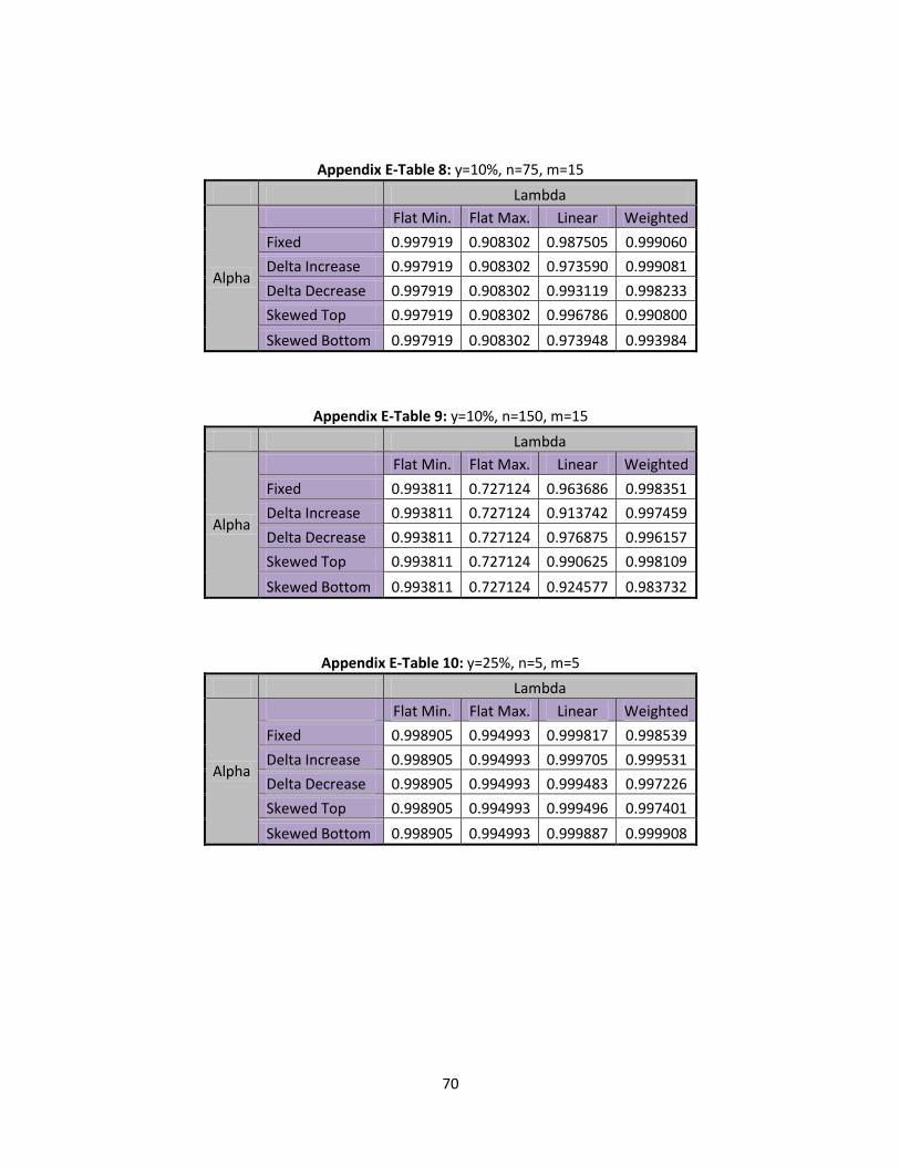
70
Appendix E-Table 8: y=10%, n=75, m=15
Lambda
Alpha
Flat Min. Flat Max. Linear Weighted
Fixed 0.997919 0.908302 0.987505 0.999060
Delta Increase 0.997919 0.908302 0.973590 0.999081
Delta Decrease 0.997919 0.908302 0.993119 0.998233
Skewed Top 0.997919 0.908302 0.996786 0.990800
Skewed Bottom 0.997919 0.908302 0.973948 0.993984
Appendix E-Table 9: y=10%, n=150, m=15
Lambda
Alpha
Flat Min. Flat Max. Linear Weighted
Fixed 0.993811 0.727124 0.963686 0.998351
Delta Increase 0.993811 0.727124 0.913742 0.997459
Delta Decrease 0.993811 0.727124 0.976875 0.996157
Skewed Top 0.993811 0.727124 0.990625 0.998109
Skewed Bottom 0.993811 0.727124 0.924577 0.983732
Appendix E-Table 10: y=25%, n=5, m=5
Lambda
Alpha
Flat Min. Flat Max. Linear Weighted
Fixed 0.998905 0.994993 0.999817 0.998539
Delta Increase 0.998905 0.994993 0.999705 0.999531
Delta Decrease 0.998905 0.994993 0.999483 0.997226
Skewed Top 0.998905 0.994993 0.999496 0.997401
Skewed Bottom 0.998905 0.994993 0.999887 0.999908
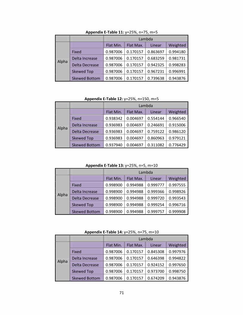
71
Appendix E-Table 11: y=25%, n=75, m=5
Lambda
Alpha
Flat Min. Flat Max. Linear Weighted
Fixed 0.987006 0.170157 0.863697 0.994180
Delta Increase 0.987006 0.170157 0.683259 0.981731
Delta Decrease 0.987006 0.170157 0.942325 0.998283
Skewed Top 0.987006 0.170157 0.967231 0.996991
Skewed Bottom 0.987006 0.170157 0.739638 0.943876
Appendix E-Table 12: y=25%, n=150, m=5
Lambda
Alpha
Flat Min. Flat Max. Linear Weighted
Fixed 0.938342 0.004697 0.554144 0.966540
Delta Increase 0.936983 0.004697 0.246691 0.915006
Delta Decrease 0.936983 0.004697 0.759122 0.986120
Skewed Top 0.936983 0.004697 0.860963 0.979121
Skewed Bottom 0.937940 0.004697 0.311082 0.776429
Appendix E-Table 13: y=25%, n=5, m=10
Lambda
Alpha
Flat Min. Flat Max. Linear Weighted
Fixed 0.998900 0.994988 0.999777 0.997555
Delta Increase 0.998900 0.994988 0.999366 0.998926
Delta Decrease 0.998900 0.994988 0.999720 0.993543
Skewed Top 0.998900 0.994988 0.999254 0.996716
Skewed Bottom 0.998900 0.994988 0.999757 0.999908
Appendix E-Table 14: y=25%, n=75, m=10
Lambda
Alpha
Flat Min. Flat Max. Linear Weighted
Fixed 0.987006 0.170157 0.845308 0.997976
Delta Increase 0.987006 0.170157 0.646398 0.994822
Delta Decrease 0.987006 0.170157 0.924152 0.997650
Skewed Top 0.987006 0.170157 0.973700 0.998750
Skewed Bottom 0.987006 0.170157 0.674209 0.943876
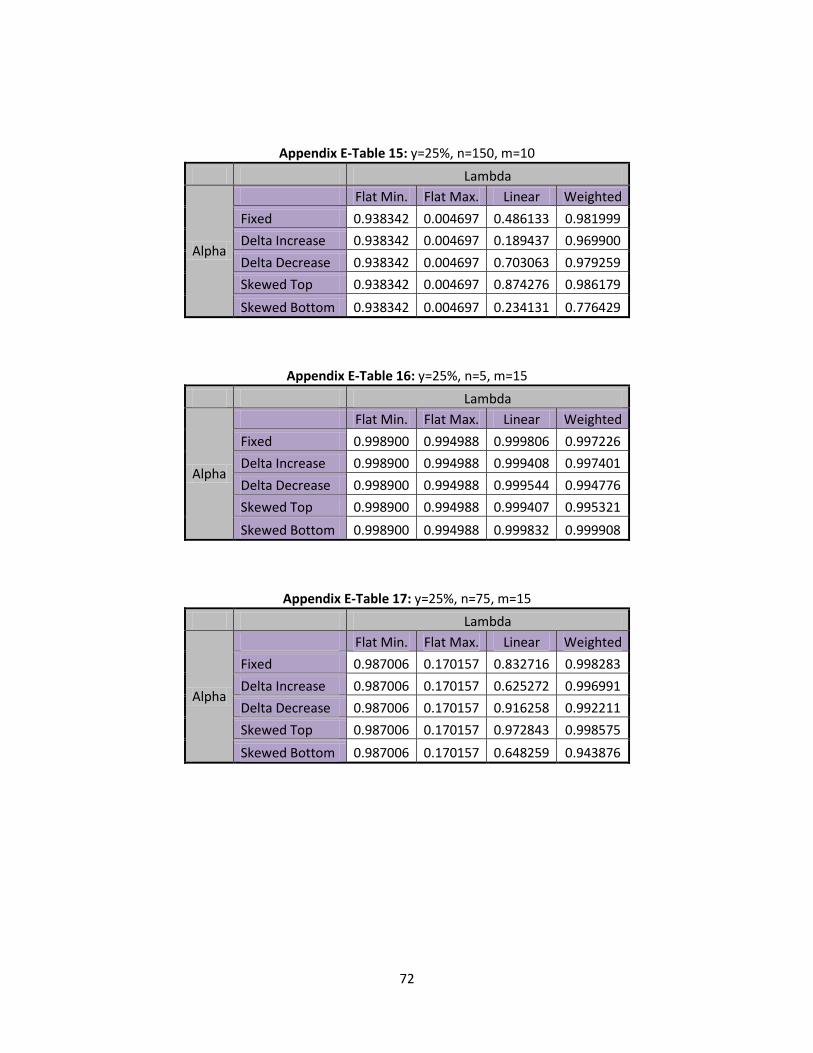
72
Appendix E-Table 15: y=25%, n=150, m=10
Lambda
Alpha
Flat Min. Flat Max. Linear Weighted
Fixed 0.938342 0.004697 0.486133 0.981999
Delta Increase 0.938342 0.004697 0.189437 0.969900
Delta Decrease 0.938342 0.004697 0.703063 0.979259
Skewed Top 0.938342 0.004697 0.874276 0.986179
Skewed Bottom 0.938342 0.004697 0.234131 0.776429
Appendix E-Table 16: y=25%, n=5, m=15
Lambda
Alpha
Flat Min. Flat Max. Linear Weighted
Fixed 0.998900 0.994988 0.999806 0.997226
Delta Increase 0.998900 0.994988 0.999408 0.997401
Delta Decrease 0.998900 0.994988 0.999544 0.994776
Skewed Top 0.998900 0.994988 0.999407 0.995321
Skewed Bottom 0.998900 0.994988 0.999832 0.999908
Appendix E-Table 17: y=25%, n=75, m=15
Lambda
Alpha
Flat Min. Flat Max. Linear Weighted
Fixed 0.987006 0.170157 0.832716 0.998283
Delta Increase 0.987006 0.170157 0.625272 0.996991
Delta Decrease 0.987006 0.170157 0.916258 0.992211
Skewed Top 0.987006 0.170157 0.972843 0.998575
Skewed Bottom 0.987006 0.170157 0.648259 0.943876
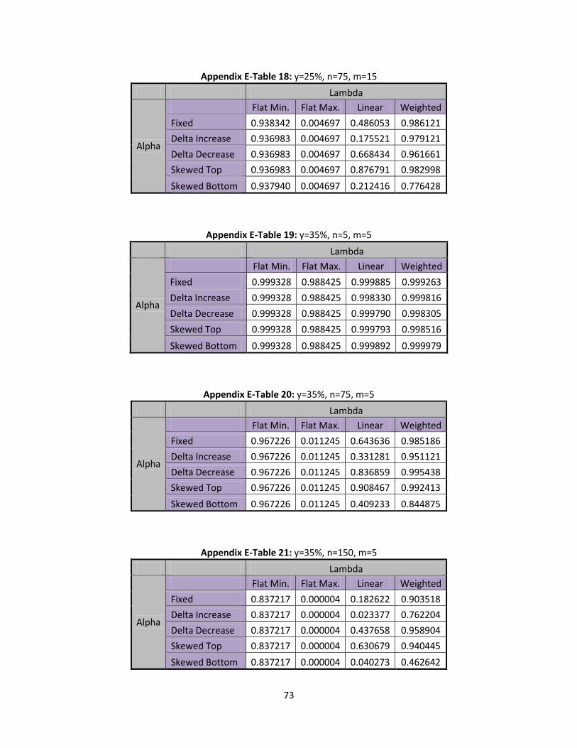
73
Appendix E-Table 18: y=25%, n=75, m=15
Lambda
Alpha
Flat Min. Flat Max. Linear Weighted
Fixed 0.938342 0.004697 0.486053 0.986121
Delta Increase 0.936983 0.004697 0.175521 0.979121
Delta Decrease 0.936983 0.004697 0.668434 0.961661
Skewed Top 0.936983 0.004697 0.876791 0.982998
Skewed Bottom 0.937940 0.004697 0.212416 0.776428
Appendix E-Table 19: y=35%, n=5, m=5
Lambda
Alpha
Flat Min. Flat Max. Linear Weighted
Fixed 0.999328 0.988425 0.999885 0.999263
Delta Increase 0.999328 0.988425 0.998330 0.999816
Delta Decrease 0.999328 0.988425 0.999790 0.998305
Skewed Top 0.999328 0.988425 0.999793 0.998516
Skewed Bottom 0.999328 0.988425 0.999892 0.999979
Appendix E-Table 20: y=35%, n=75, m=5
Lambda
Alpha
Flat Min. Flat Max. Linear Weighted
Fixed 0.967226 0.011245 0.643636 0.985186
Delta Increase 0.967226 0.011245 0.331281 0.951121
Delta Decrease 0.967226 0.011245 0.836859 0.995438
Skewed Top 0.967226 0.011245 0.908467 0.992413
Skewed Bottom 0.967226 0.011245 0.409233 0.844875
Appendix E-Table 21: y=35%, n=150, m=5
Lambda
Alpha
Flat Min. Flat Max. Linear Weighted
Fixed 0.837217 0.000004 0.182622 0.903518
Delta Increase 0.837217 0.000004 0.023377 0.762204
Delta Decrease 0.837217 0.000004 0.437658 0.958904
Skewed Top 0.837217 0.000004 0.630679 0.940445
Skewed Bottom 0.837217 0.000004 0.040273 0.462642
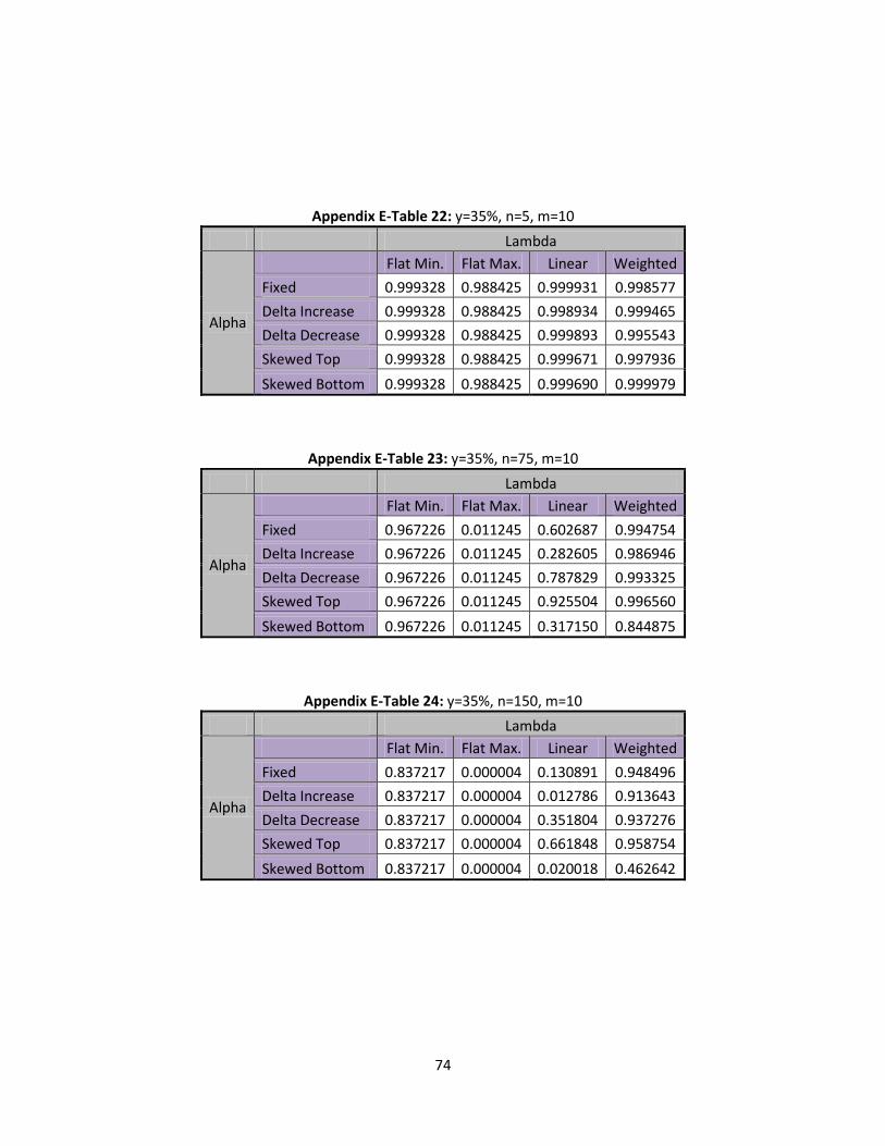
74
Appendix E-Table 22: y=35%, n=5, m=10
Lambda
Alpha
Flat Min. Flat Max. Linear Weighted
Fixed 0.999328 0.988425 0.999931 0.998577
Delta Increase 0.999328 0.988425 0.998934 0.999465
Delta Decrease 0.999328 0.988425 0.999893 0.995543
Skewed Top 0.999328 0.988425 0.999671 0.997936
Skewed Bottom 0.999328 0.988425 0.999690 0.999979
Appendix E-Table 23: y=35%, n=75, m=10
Lambda
Alpha
Flat Min. Flat Max. Linear Weighted
Fixed 0.967226 0.011245 0.602687 0.994754
Delta Increase 0.967226 0.011245 0.282605 0.986946
Delta Decrease 0.967226 0.011245 0.787829 0.993325
Skewed Top 0.967226 0.011245 0.925504 0.996560
Skewed Bottom 0.967226 0.011245 0.317150 0.844875
Appendix E-Table 24: y=35%, n=150, m=10
Lambda
Alpha
Flat Min. Flat Max. Linear Weighted
Fixed 0.837217 0.000004 0.130891 0.948496
Delta Increase 0.837217 0.000004 0.012786 0.913643
Delta Decrease 0.837217 0.000004 0.351804 0.937276
Skewed Top 0.837217 0.000004 0.661848 0.958754
Skewed Bottom 0.837217 0.000004 0.020018 0.462642
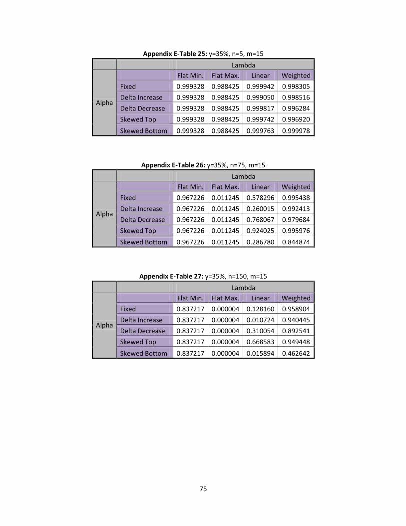
75
Appendix E-Table 25: y=35%, n=5, m=15
Lambda
Alpha
Flat Min. Flat Max. Linear Weighted
Fixed 0.999328 0.988425 0.999942 0.998305
Delta Increase 0.999328 0.988425 0.999050 0.998516
Delta Decrease 0.999328 0.988425 0.999817 0.996284
Skewed Top 0.999328 0.988425 0.999742 0.996920
Skewed Bottom 0.999328 0.988425 0.999763 0.999978
Appendix E-Table 26: y=35%, n=75, m=15
Lambda
Alpha
Flat Min. Flat Max. Linear Weighted
Fixed 0.967226 0.011245 0.578296 0.995438
Delta Increase 0.967226 0.011245 0.260015 0.992413
Delta Decrease 0.967226 0.011245 0.768067 0.979684
Skewed Top 0.967226 0.011245 0.924025 0.995976
Skewed Bottom 0.967226 0.011245 0.286780 0.844874
Appendix E-Table 27: y=35%, n=150, m=15
Lambda
Alpha
Flat Min. Flat Max. Linear Weighted
Fixed 0.837217 0.000004 0.128160 0.958904
Delta Increase 0.837217 0.000004 0.010724 0.940445
Delta Decrease 0.837217 0.000004 0.310054 0.892541
Skewed Top 0.837217 0.000004 0.668583 0.949448
Skewed Bottom 0.837217 0.000004 0.015894 0.462642