Statistical Thermodynamics: Introduction to Phase … · Statistical Thermodynamics: Introduction to Phase Space and Metastable States Phase Space and Metastable States for the Ising

Statistical Thermodynamics: Introduction to Phase Space and Metastable States

Phase Space and Metastable States for the Ising Spin Glass

with Interactive Enthalpy: A White Paper

Alianna J. Maren, Ph.D.

Themasis

February, 2014

Initiated December, 2009; modified November, 2011

THM TR2014-001(ajm)

1 Goal of This Paper

This paper overviews the phase space diagram for the simple Ising glass model with interacting

enthalpy between neighboring units. It presents the free energy diagrams for different parameter

combinations, and shows how metastable states can exist, with the potential for cascading from a

metastable state to a stable one. It very briefly identifies some realms of social phenomena where

the metastable state model may prove useful.

By understanding how enthalpy and entropy interact in a simple system, we observe the impacts

of each term, and can better understand both the usefulness and limitations of this model.

This understanding paves the way for recognizing why more complex models will be needed,

and to establish exactly what we would desire from a more complex model that is not available

in the simple Ising system.

2 Background

Statistical mechanics, particularly the simple Ising model with a stabilizing interactive energy

between like pairs, has potential to model a number of phenomena. The key to making this

model useful is to understand how the free energy changes as a function of the two key

parameters in a reduced representation; the (reduced) enthalpy per unit in the “active” state, and

the interaction enthalpy term.

2

Feb. 27, 2014 Statistical Mechanics: Phase Spaces & Metastable States THM Technical Report

A previous White Paper, Statistical Thermodynamics: Basic Theory and Equations1, presented

the equations that are briefly summarized in this work.

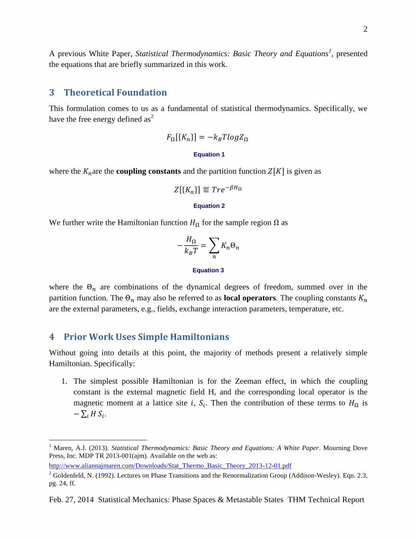
3 Theoretical Foundation

This formulation comes to us as a fundamental of statistical thermodynamics. Specifically, we

have the free energy defined as2

Equation 1

where the are the coupling constants and the partition function is given as

Equation 2

We further write the Hamiltonian function for the sample region as

Equation 3

where the are combinations of the dynamical degrees of freedom, summed over in the

partition function. The may also be referred to as local operators. The coupling constants

are the external parameters, e.g., fields, exchange interaction parameters, temperature, etc.

4 Prior Work Uses Simple Hamiltonians

Without going into details at this point, the majority of methods present a relatively simple

Hamiltonian. Specifically:

1. The simplest possible Hamiltonian is for the Zeeman effect, in which the coupling

constant is the external magnetic field H, and the corresponding local operator is the

magnetic moment at a lattice site , . Then the contribution of these terms to is

.

1 Maren, A.J. (2013). Statistical Thermodynamics: Basic Theory and Equations: A White Paper. Mourning Dove

Press, Inc. MDP TR 2013-001(ajm). Available on the web as:

http://www.aliannajmaren.com/Downloads/Stat_Thermo_Basic_Theory_2013-12-01.pdf 2 Goldenfeld, N. (1992). Lectures on Phase Transitions and the Renormalization Group (Addison-Wesley). Eqn. 2.3,

pg. 24, ff.

http://www.aliannajmaren.com/Downloads/Stat_Thermo_Basic_Theory_2013-12-01.pdf

3


2. Introducing a nearest-neighbor spin interaction energy produces the nearest-neighbor

Ising model Hamiltonian, which is:

Equation 4

where we assume a uniform magnetic field H, and the notation <ij> means that “i and j

are nearest neighbor sites”. refers to the spin on a site; in the Ising model, we allow for

two spin alternatives, resulting in two possible states, A or B. (Spin up or down, or active

/ non-active, etc.) In this model, the only interaction between spins is the nearest-

neighbor interaction, denoted by J.

In many attempts to apply statistical mechanics to neural networks and related areas, the methods

do not explicitly show the free energy contribution made by the entropy term. That is, these

methods do explicitly show the enthalpy component, but not the configurational component.

5 Introducing Configurational Free Energy: The Entropy Term

There is an astoundingly good reason why previous formulations do not include the entropy

term. When we use a simple bistate model, specifically, the simple Ising model, we do not gain

any “model advantage” to our formulation. If anything, the situation becomes much worse!

To understand this, we need to examine the behavior of a simple entropy term, and what happens

when we introduce it into the system model.

From Hill, Statistical Mechanics3, we recapitulate the basics

4:

The basic equation from simple thermodynamics for the Helmholtz Free Energy is given as:

where F is the Helmholtz free energy, U is the enthalpy, or energy associated with those units in

an “active” state, T is the temperature, and S is the entropy.

In differential form

3Hill, T.L. (1956), Statistical Mechanics (McGraw-Hill). Section 41, pgs 288 ff.

See also: http://en.wikipedia.org/wiki/Helmholtz_free_energy, http://en.wikipedia.org/wiki/Gibbs_free_energy,

http://hyperphysics.phy-astr.gsu.edu/hbase/thermo/helmholtz.html 4 The notation in this paper and in the previous work is drawn from Hill (ref. 3) and Goldenfeld (ref. 2); the previous

White Paper (ref. 1) includes a Table showing correspondences between notation in these two sources.

http://en.wikipedia.org/wiki/Helmholtz_free_energy

http://en.wikipedia.org/wiki/Gibbs_free_energy

http://hyperphysics.phy-astr.gsu.edu/hbase/thermo/helmholtz.html

4


where is an external magnetic field, or consistently maintained stimulus. (In our work, we will

take this stimulus to be a search or query imposed on a corpus containing items that potentially

respond to this stimulus by changing from an “inactive” state A into an “active” state B.

Since (the free energy) and other terms are extensive quantities, we create the term to refer

to the Helmholtz energy per unit, or to create an intensive quantity, and similarly for the other

variables. (Note that this corresponds to f of the immediately preceding Goldenfeld notation.)

is an external parameter (NOTE that this is a script , not the simple italic used for free

energy; this is infusing the Goldenfeld notation into Hill’s notation.) replaces the volume in

ordinary thermodynamics, and comparable to intensity of magnetization, or total “activated

strength” associated with the number of “active” units responding to stimulus) and is an

extensive quantity. (In our application, this can be related to corpus size.) We use to represent

the external, consistently maintained stimulus. This can be a magnetic field, when considering a

ferromagnetic system, or a sustained “search” or “query” activation, for our application. (Note

that if presenting the query does not change our analog to “system volume,” then this term

goes to zero.)

Finally, is normally the chemical potential; here we treat it as the energy that can be associated

with a unit in its activated state, and is the total number of units (A+B=N) in the system.

We note that as , or that as the external stimulus becomes very large, the total

number of units in the “activated” state A approaches the total number of units N. The reverse, as

, is also true.

6 The Impact of Introducing a Simple Entropy Formulation

A simple bistate system is most often treated as a “spin glass,” modeled by the Ising equations,

which provide a Helmholtz Free Energy5. The simple equation for this situation, again using a

bistate system wherein the fraction of units in an “activated state” is x, and the remaining

fraction, 1-x, is in an “inactive state” is given as:

Equation 5

where F is the Helmholtz free energy, U is the enthalpy, or energy associated with those units in

an “active” state, T is the temperature, and S is the entropy.

5http://en.wikipedia.org/wiki/Helmholtz_free_energy, http://en.wikipedia.org/wiki/Gibbs_free_energy,


http://en.wikipedia.org/wiki/Helmholtz_free_energy

http://en.wikipedia.org/wiki/Gibbs_free_energy


5


We first compute the entropy term and examine its influence on the free energy for a simple bi-

state system, and then examine the influence of a slightly more complex (spin-pair interaction)

enthalpy when the entropy is included.

6.1 Analytic Properties; Computing the Entropy

From the preceding differential form of the free energy equation, we can write the entropy as6

Equation 6

where

Equation 7

We consider a bi-state system, and allow the fraction of items in state A to be x, so the remaining

fraction in state B is 1-x. We divide the preceding entropy equation through by the various

entropy coefficients associated to obtain a reduced entropy expression:

.

Equation 8

We notice that , so that . Thus, the and

although becomes undefined as , . Thus

we have that S is a convex function, where when x = 0.5.

6.2 Introducing Entropy into the Free Energy Formulation

No matter how we scale the entropy term S, when we add the negative entropy to the free energy

equation, we introduce a term that pushes the free energy minimum to the case where x = 0.5.

The enthalpy components of the free energy “modulate” the minimum, pushing it to the left or

6 For derivations, see Themis White Paper Statistical Thermodynamics: Basic Theory and Equations, Themis

TR2009-001(ajm).

6


right. However, it takes a very large enthalpy component to shift the free energy minimum

significantly from x = 0.5, once the entropy has been introduced.

6.3 The Role of Temperature

When we look at the free energy equation, we see that raising the temperature T causes the

entropy term (-TS) to become a deeper concave curve. (Entropy itself is maximum when x=0.5

for the case where activation and interaction parameters, or enthalpy, are zero.)

This means that increasing temperature drives the system minimum to be more governed by

entropy.

However, we do not have an exact corollary for “temperature” when we apply this model to

document corpora. Thus, we work with the “reduced” free energy equation, in which the

temperature and other coefficients are absorbed. We can then study the phenomenology in a

clearer manner.

7 The Full Free Energy Equation

7.1 The Reduced Enthalpy Term

The first RHS term in Equation 5 is the enthalpy term, U, given as:

Equation 9

The reduced version is divided through by T, giving:

Equation 10

Before engaging in the detailed equations, we offer some notes about the key parameters, and

. The first parameter, , deals with the increase in activation energy of the “active fraction” of

nodes relative to the inactive ones.

When we create a reduced free energy equation, the early parameters for e1 and e2 are now

divided by T, resulting in the parameters and . An increase in T reduces both and .

7.2 Activation Energy Parameter

The first parameter, , deals with the increase in activation energy of the “active fraction” of

nodes relative to the inactive ones. Thus, increasing T is the same as reducing e1, or the energy

7


difference between an active node and a non-active one. Conversely, increasing is equivalent

to either reducing T or to increasing the energy difference between active and non-active nodes.

Either way, increasing shifts the free energy minimum (at least, for simple versions of the free

energy equation) to states where the equilibrium state requires fewer active nodes.

This only carries us so far. Systems with only activation energy, and no interaction energy, are

not very interesting. In the simple Ising model (with simple state distribution entropy, not

considering the effect of cluster distributions), there is just a single minimum when there is no

interaction energy. State transitions are smooth, and not particularly interesting. This is not a

useful or interesting model for our purposes of modeling information systems.

7.3 Introducing Spin-Pair Interaction Energies

Things become a bit more interesting when we introduce the pairwise interaction energy term –

both for simple and complex energy terms. We typically assign a negative value to the

interaction energy; is negative. The physical meaning of this is that an interaction between

similar terms (between, e.g., two active nodes) reduces the overall free energy of the system.

That means that the interaction between two neighboring active nodes is a stabilizing force for

equilibrium.

This further means that as we increase the (negative) value of , we get a more pronounced

difference in the effect of having nodes in the active versus nonactive states. Even for the simple-

entropy version, we get a rather complex phase diagram. For our work with the more complex

entropy, we shall simply keep in mind that increasing the (negative) interaction energy promotes

formation of clusters, because it precisely this interaction energy that causes clusters to persist.

7.4 The Full Free Energy Equation

We substitute Equation 8 and Equation 10 into Equation 5 (this includes prior division through

by T and the various entropy associated coefficients) to obtain a reduced free energy expression:

.

Equation 11

In this equation, the two epsilon terms refer to the energy associated with the active units (ε1) and

the interaction energy (where we have used ε2 /2 as the interaction energy term for simplicity,

given how the following equation resolves). The term on the far right is the (reduced) Canonical

Ensemble, which will give us a set of simpler terms in the following equation.

In nature, all systems tend towards a minimal free energy state. To compute this, we take the

derivative of Equation 11 with respect to x, the fraction of “active” units, and set it equal to zero.

8


Equation 12

8 The Phase Space Diagram for the Simple Ising Spin Glass

Figure 1 shows the phase diagram for the system described in Equation 12.7

Figure 1: Phase diagram for simple bi-state Ising model in terms of the reduced parameters, ε1 and a = ε2/ ε1.

The following Table characterizes each of these phase-space regions.

Region Number of

Minima

Description

A 1 Single minimum exists for very small values of x (x << 0.1)

B N/A Extreme behavior; unsuitable for modeling

C 1 Single broad, very shallow minimum

D 2 Two minima of various depths relative to separating central

maximum

E N/A Extreme behavior; unsuitable for modeling

F 1 Single minimum exists, when x is large (0.9 < x < 1.0)

G 1 Very similar to region F, but the values of x are so close to 1

that essentially all units are “active” or in the “on” state

Table 1: Regions in the bistate Ising Spin Glass

7 Figure based on work originally presented in A.J. Maren, Theoretical Models for Solid-State Phase Transitions,

Doctoral Dissertation, Arizona State University, 1981. Figure reproduced with assistance from Eyal Schwartz in the

summer of 1994 at Radford University. Financial support from the Jeffries Foundation is gratefully acknowledged.

9


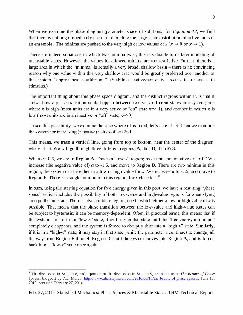
When we examine the phase diagram (parameter space of solutions) for Equation 12, we find

that there is nothing immediately useful in modeling the large-scale distribution of active units in

an ensemble. The minima are pushed to the very high or low values of x ( ).

There are indeed situations in which two minima exist; this is valuable to us later modeling of

metastable states. However, the values for allowed minima are too restrictive. Further, there is a

large area in which the “minima” is actually a very broad, shallow basin – there is no convincing

reason why one value within this very shallow area would be greatly preferred over another as

the system “approaches equilibrium.” (Stabilizes active/non-active states in response to

stimulus.)

The important thing about this phase space diagram, and the distinct regions within it, is that it

shows how a phase transition could happen between two very different states in a system; one

where x is high (most units are in a very active or “on” state x=> 1), and another in which x is

low (most units are in an inactive or “off” state, x=>0).

To see this possibility, we examine the case where ε1 is fixed; let’s take ε1=3. Then we examine

the system for increasing (negative) values of a=ε2/ε1.

This means, we trace a vertical line, going from top to bottom, near the center of the diagram,

where ε1=3. We will go through three different regions; A, then D, then F/G.

When a=-0.5, we are in Region A. This is a “low x” region; most units are inactive or “off.” We

increase (the negative value of) a to -1.5, and move to Region D. There are two minima in this

region; the system can be either in a low or high value for x. We increase a to -2.5, and move to

Region F. There is a single minimum in this region, for x close to 1.8

In sum, using the starting equation for free energy given in this post, we have a resulting “phase

space” which includes the possibility of both low-value and high-value regions for x satisfying

an equilibrium state. There is also a middle region, one in which either a low or high value of x is

possible. That means that the phase transition between the low-value and high-value states can

be subject to hysteresis; it can be memory-dependent. Often, in practical terms, this means that if

the system starts off in a “low-x” state, it will stay in that state until the “free energy minimum”

completely disappears, and the system is forced to abruptly shift into a “high-x” state. Similarly,

if it is in a “high-x” state, it may stay in that state (while the parameter a continues to change) all

the way from Region F through Region D, until the system moves into Region A, and is forced

back into a “low-x” state once again.

8 The discussion in Section 8, and a portion of the discussion in Section 9, are taken from The Beauty of Phase

Spaces, blogpost by A.J. Maren, http://www.aliannajmaren.com/2010/06/17/the-beauty-of-phase-spaces/, June 17,

2010, accessed February 27, 2014.

http://www.aliannajmaren.com/2010/06/17/the-beauty-of-phase-spaces/

10


9 Metastable States and Hysteresis in the Ising Spin Glass

To understand the free energy equilibrium points as given by Equation 12, we first examine the

actual reduced free energy, shown in Figure 2.9

Figure 2: Set of five free energy graphs; F* versus x, where F* is the “reduced” (re-parameterized) free energy, and x represents the fraction of units in the system in an “on” or “activated” state. The five different graphs are obtained for different combinations of enthalpy parameters (to be discussed in a following post). The topmost graph refers to Region A (see following Figure 2), in which only a single free energy minimum exists, and is for a low value of x. The middle three graphs are for parameter values taken from Region D of

Figure 2; these allow for double minima to appear. That means that a system can be in either a low-x or high-x state. (Relatively few activated units, or almost all units active.) The lowest graph corresponds to Region F,

for which only a single free energy minimum exists, but this time with a high value of x (most units are “active” or “on.”)

9 Figure from Alianna J. Maren, Theoretical Models for Solid-State Phase Transitions, Doctoral Dissertation,

Arizona State University, 1981.

11


9.1 Hysteresis Can Occur When Moving Through this Phase Space

Solving for the free energy equilibrium Equation 12 explains hystersis as well as phase

transitions in memory-dependent systems, such as ferromagnets. In this case, a ferromagnetic

material that is disordered (different domains are randomly aligned) will become ordered (almost

all the domains will align their magnetic fields) when put into an external magnetic field. They

will maintain their alignment for a long time. It will take a significant change in external

circumstances (e.g., raising the temperature a great deal) to destroy the alignment and bring the

ferromagnet back into a disordered state once again. Then, a lot of effort (a significant magnetic

field) would be required to re-align the domains.

Figure 3: Bistate Ising Spin Glass Phase Space (on which Figure 1 is based); actual screen shot of computed distinct free energy curve natures, see Table 1 for space labels A .. G.

Figure 3 shows a “path” going from a low-active state (1) to a high-active state (3) back to low-

active state (7) again.10

We start our walkthrough with being at Point 1 of Figure 3, in Region A. Region A is the area

where there is only one free energy minimum. That means, there is only one “stable state.” For

Region A, this minimum occurs for a relatively low value of x, as is shown in the following

Figure x.11

10

This figure was originally presented in Tracing the Financial Meltdown of 2008-9, blogpost by A.J. Maren,

http://www.aliannajmaren.com/2011/06/08/tracing-the-financial-meltdown-of-2008-9/, June 8, 2011, accessed

February 27, 2014. 11

This portion of the discussion in Section 9 is taken from "What is X?" – Modeling the Meltdown, blogpost by A.J.

Maren, http://www.aliannajmaren.com/2011/06/09/what-is-x-modeling-the-meltdown/, June 9, 2011, accessed

February 27, 2014.

http://www.aliannajmaren.com/2011/06/08/tracing-the-financial-meltdown-of-2008-9/

http://www.aliannajmaren.com/2011/06/09/what-is-x-modeling-the-meltdown/

12


Figure 4: Illustrative reduced free energy for phase space Region A: single free energy minimum (with low value for x).

12

9.2 Interpretation: What Is the Influence of the Enthalpy Parameters?

We can see that in this Figure 4 (characteristic for all of Region A), the value of x giving the free

energy minimum is about at x=0.1.

If we’re going to apply this model, we now need to identify the meaning of the two parameters

involved; ε1 and a = ε2/ ε1.

When we look at the phase space diagrams of Figure 1 and Figure 3, we see that there are two

parameters. The one across the top (ranging from 1.5 to 8.5) is ε1. ε1 represents an “activation

energy,” or the “energy cost” (enthalpy per unit) of having a unit in an active state.

Let’s have a quick review of basic thermodynamic principles. A system is “at equilibrium” when

the free energy at a minimum. (In Figure 4, this occurs when x is about 0.1.) Free energy is

enthalpy minus (a constant times) entropy. (We worked with the “reduced” free energy in all of

our discussions, where constants and other terms have been divided out, subtracted out, or

otherwise normalized; so all future references to enthalpy will really mean a “reduced” enthalpy

where various constants have been worked to give a simpler, cleaner equation.)

12

Figure from Alianna J. Maren, Theoretical Models for Solid-State Phase Transitions, Doctoral Dissertation,

Arizona State University, 1981, and presented in "What is X?" – Modeling the Meltdown, blogpost by A.J. Maren,

http://www.aliannajmaren.com/2011/06/09/what-is-x-modeling-the-meltdown/, June 9, 2011, accessed February 27,

2014.

http://www.aliannajmaren.com/2011/06/09/what-is-x-modeling-the-meltdown/

13


As per Equation 9 and Equation 10, we really have two enthalpy terms; one is an enthalpy-per-

active unit (linear in x), and the other is an interaction energy term, which is an “interaction

energy” times x-squared.

The enthalpy-per-active-unit is ε1.

If we’re going to make this model work, we need to figure out what this means.

Suppose that we took our basic free energy equation, and pretended that there was no enthalpy at

all; there was no extra “energy” put into the system when the various units were “on” or “off.”

Then the free energy would be at a minimum when the entropy was at a maximum, and this

occurs when x=0.5. (The entropy equation here is symmetric; entropy = x(ln(x)+(1-x)ln(1-x).

What happens when we introduce the enthalpy terms is that we “skew” the free energy minimum

to one side or another. Region A corresponds to the area where the interaction energy is low, so

for the moment, let’s pretend that it doesn’t exist. We’ll focus on the physical meaning of the

parameter ε1. It is to be something that will shift the free energy minimum to the left, or make the

value of x that produces a free energy minimum to be smaller. (Figure 4, the free energy is at a

minimum when x=0.1 instead of 0.5.)

The enthalpy-per-unit term, ε1, associated with Region A (and in fact all of Figure 1) is a positive

term. It means that there is an “energy cost” to having a unit in an active state.

9.3 Illustrative Application to Financial Systems (2008-2009 Crash)

An example application: In modeling financial scenarios, we could interpret this cost as risk. In

such a case, we would say that ε1 models the risk for a unit (a bank, a hedge fund, etc.) to be

involved in a very leveraged transaction. The risk can be small (ε1 =2) or large (ε1 =7). Either

way, we get a single minimum if there is no “interaction” energy; this minimum is for a low

value of x, meaning that relatively few units are “on” or are involved in risky transactions.

Now we come to the “crux of the biscuit.” What does the other parameter, a, mean? This is our

interaction-energy term; it multiplies x-squared.

We get the “interesting behavior” in Region D (the middle, pink region of the phase space

diagram of Figure 3). And in order to get the system to move from what we’d think of as a

“logical, sane” equilibrium state – one in which relatively few units are involved in risky

transactions – to the equilibrium state of Regions F or G (where most of the units are “on”) –

something has to happen. Something has to “force” more units to take on more “risk.”

This “something” has to do with how the units interact with each other.

What would this mean in Wall Street social and political dynamics? How about peer pressure?

Think about it. Interaction-energy = peer pressure. This is how banks and other institutions –

who knew that what they were doing was not only risky, but downright foolhardy – were moving

into these highly leveraged situations.

14


In terms of Figure 3, the whole system of Wall Street financial institutions were going from

Point 1 to Point 2 to Point 3. By the time the system was in Point 3 (metastable state in Region

F, one of the stable values for x approximately 0.9), almost all units were involved in risky

transactions (see the free energy diagram in Figure 2), and the “free energy minimum” was

VERY deep.

And there was no “alternative.” By the time the system was in Region F, there was only a single

free energy minimum. In other words, the whole system was trapped in a very risky situation.

9.4 The Return Loop on Hysteresis: When the Metastable State Crashes

The most important thing to note right now is that – both in the model predictions AND in the

real-world events that we’ve been observing – meltdowns happen fast. We can be in a metastable

state that lasts so long, and is so extreme, that many people believe that the situation will last

forever.13

But it doesn’t.

Consider the return loop. Start with a system at Point 3, in Region F. (See Figure 3). This is

when a system has “tipped” so that almost all units are in State B. (For purposes of our model,

we’re identifying State B as being “highly risky.”) Now, suppose that the enthalpy (the energy

put into the system) to keep these units in State B starts being withdrawn. The system can persist

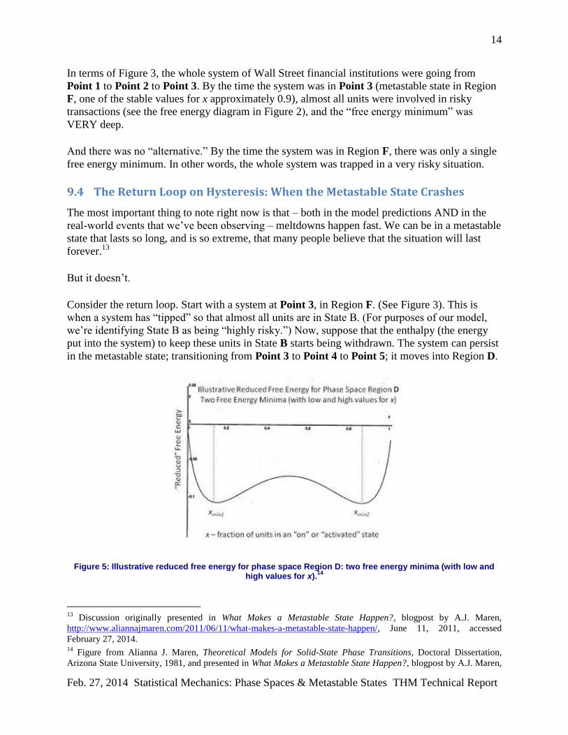
in the metastable state; transitioning from Point 3 to Point 4 to Point 5; it moves into Region D.

Figure 5: Illustrative reduced free energy for phase space Region D: two free energy minima (with low and high values for x).

14

13

Discussion originally presented in What Makes a Metastable State Happen?, blogpost by A.J. Maren,

http://www.aliannajmaren.com/2011/06/11/what-makes-a-metastable-state-happen/, June 11, 2011, accessed

February 27, 2014. 14

Figure from Alianna J. Maren, Theoretical Models for Solid-State Phase Transitions, Doctoral Dissertation,

Arizona State University, 1981, and presented in What Makes a Metastable State Happen?, blogpost by A.J. Maren,

http://www.aliannajmaren.com/2011/06/11/what-makes-a-metastable-state-happen/

15


A metastable state can collapse quickly.

Envision the case where a system moves from Point 3 to Point 4 to Point 5, shown in Figure 3.

At Point 3, the value for x is high (about 0.9). As it moves towards Point 5, it is in Region D.

Region D is the realm in which metastabilities exist. That means that there are two free energy

minima, throughout all points in Region D. (If you’ll refer to the phase diagram of Figure 3,

you’ll see that Region D is the pink area in the middle; bordered by Region A at the top and

Region G below, where both A and G are light blue.)

The system goes through the free energy states shown in Figure 2, on the right-hand side. The

most stable value for x (lowest point on the free energy curve) gradually becomes very unstable,

and a slight parameter change (moving the value of a = ε2/ ε1 closer to 0) shifts the whole system

into Region A once again – the region from which the whole cycle started.

Once again, the only stable state for the system is when x is very small (about 0.1). This shift in x

values, from large to small, can happen very fast once the metastability no longer holds.

In a previous section (Illustrative Application to Financial Systems (2008-2009 Crash)), I

characterized the interaction energy a as peer pressure – an interaction that caused active units to

“encourage” other units to be active.

The metastable state is reached when the peer pressure is reduced – public awareness grows,

many people start describing the overall system as highly risky, and the support given by one

institution (or set of highly-leveraged loans) to encourage another is greatly reduced. The

“encouragement” is strong when the parameter a takes on a large negative value (e.g., -3).

When parameter a moves back towards zero (peer pressure to stay in a high-risk situation is

relieved), the system moves back to the state in which only a few institutions offer highly-

leveraged, high-risk options. The shift can be very sudden and dramatic.

The financial meltdown of 2008-2009, beginning with the Lehman Brothers, is a case in point.

10 Summary

Statistical mechanics – even in simple form; the bistate Ising spin glass with simple entropy –

can usefully model not only physical systems but also - potentially – social ones as well. In

particular, the model discussed here could be applied to social systems that go through rapid

changes, which may be described as moving out of a metastable state.

One of the most interesting possibilities is whether or not statistical mechanics can be usefully

applied to large data corpora.

http://www.aliannajmaren.com/2011/06/11/what-makes-a-metastable-state-happen/, June 11, 2011, accessed

February 27, 2014.

http://www.aliannajmaren.com/2011/06/11/what-makes-a-metastable-state-happen/

16


In the context of the phase space analysis given here, the answer is: for most applications, not

yet. The model is still too simplistic to be useful. (This is likely why applications have not yet

been made.)

A subsequent White Paper will introduce a more advanced statistical thermodynamics model;

one which potentially can be applied to challenges such as data analytics for large data corpora.

11 Research Bibliography

Goldenfeld, N. (1992). Lectures on Phase Transitions and the Renormalization Group (Addison-

Wesley).

Hill, T.L. (1956), Statistical Mechanics (McGraw-Hill).

Maren, A.J. (2013). Statistical Thermodynamics: Basic Theory and Equations: A White Paper.

Mourning Dove Press, Inc. MDP TR 2013-001(ajm). Available on the web as:


A.J. Maren (1981). Theoretical Models for Solid-State Phase Transitions, Doctoral Dissertation,

Arizona State University.

Schwartz, E., & Maren, A.J. (1994). Domains of interacting neurons: A statistical mechanical

model, in Proc. World Congress on Neural Networks (WCNN).


Documents

Statistical Thermodynamics: Introduction to Phase … · Statistical Thermodynamics: Introduction to Phase Space and Metastable States Phase Space and Metastable States for the Ising