Embed Size (px)
Citation preview
Statistical hypothesis testing http://en.wikipedia.org/w/index.php?title=Statistical_hypothesis_testing&printable=yes
A statistical hypothesis test is a method of statistical inference using data from
a scientific study. In statistics, a result is called statistically significant if it has been
predicted as unlikely to have occurred bychance alone, according to a pre-determined
threshold probability, the significance level. The phrase "test of significance" was
coined by statistician Ronald Fisher.[1] These tests are used in determining what
outcomes of a study would lead to a rejection of the null hypothesis for a pre-specified
level of significance; this can help to decide whether results contain enough
information to cast doubt on conventional wisdom, given that conventional wisdom
has been used to establish the null hypothesis. The critical region of a hypothesis test
is the set of all outcomes which cause the null hypothesis to be rejected in favor of
the alternative hypothesis. Statistical hypothesis testing is sometimes
called confirmatory data analysis, in contrast to exploratory data analysis, which
may not have pre-specified hypotheses. In the Neyman-Pearson framework (see
below), the process of distinguishing between the null & alternative hypotheses is
aided by identifying two conceptual types of errors (type 1 & type 2), and by
specifying parametric limits on e.g. how much type 1 error will be permitted.
Contents
1 Variations and sub-classes
2 The testing process
2.1 Interpretation
2.2 Use and importance
2.3 Cautions
3 Example
3.1 Lady tasting tea
3.2 Analogy – Courtroom trial
3.3 Example 1 – Philosopher's beans
3.4 Example 2 – Clairvoyant card game
3.5 Example 3 – Radioactive suitcase
4 Definition of terms
5 Common test statistics
6 Origins and early controversy
6.1 Early choices of null hypothesis
7 Null hypothesis statistical significant testing vs hypothesis testing
8 Criticism
8.1 Alternatives to significance testing
9 Philosophy
10 Education
11 See also
12 References
13 Further reading
14 External links
Variations and sub-classes
Statistical hypothesis testing is a key technique of both Frequentist
inference and Bayesian inference although they have ×notable differences. Statistical
hypothesis tests define a procedure that controls (fixes) the probability of
incorrectly deciding that a default position (null hypothesis) is incorrect based on how
likely it would be for a set of observations to occur if the null hypothesis were true.
Note that this probability of making an incorrect decision is not the probability that
the null hypothesis is true, nor whether any specific alternative hypothesis is true. This
contrasts with other possible techniques of decision theory in which the null
and alternative hypothesis are treated on a more equal basis. One
naive Bayesian approach to hypothesis testing is to base decisions on the posterior
probability,[2][3] but this fails when comparing point and continuous hypotheses. Other
approaches to decision making, such as Bayesian decision theory, attempt to balance
the consequences of incorrect decisions across all possibilities, rather than
concentrating on a single null hypothesis. A number of other approaches to reaching a
decision based on data are available via decision theory and optimal decisions, some
of which have desirable properties, yet hypothesis testing is a dominant approach to
data analysis in many fields of science. Extensions to the theory of hypothesis testing
include the study of the power of tests, the probability of correctly rejecting the null
hypothesis given that it is false. Such considerations can be used for the purpose
of sample size determination prior to the collection of data.
The testing process
In the statistics literature, statistical hypothesis testing plays a fundamental role.[4] The
usual line of reasoning is as follows:
1. There is an initial research hypothesis of which the truth is unknown.
2. The first step is to state the relevant null and alternative hypotheses. This is
important as mis-stating the hypotheses will muddy the rest of the process.
Specifically, the null hypothesis allows to attach an attribute: it should be
chosen in such a way that it allows us to conclude whether the alternative
hypothesis can either be accepted or stays undecided as it was before the test.[5]
3. The second step is to consider the statistical assumptions being made about the
sample in doing the test; for example, assumptions about the statistical
independence or about the form of the distributions of the observations. This is
equally important as invalid assumptions will mean that the results of the test
are invalid.
4. Decide which test is appropriate, and state the relevant test statistic T.
5. Derive the distribution of the test statistic under the null hypothesis from the
assumptions. In standard cases this will be a well-known result. For example
the test statistic might follow a Student's t distribution or a normal distribution.
6. Select a significance level (α), a probability threshold below which the null
hypothesis will be rejected. Common values are 5% and 1%.
7. The distribution of the test statistic under the null hypothesis partitions the
possible values of T into those for which the null hypothesis is rejected, the so-
called critical region, and those for which it is not. The probability of the
critical region is α.
8. Compute from the observations the observed value tobs of the test statistic T.
9. Decide to either reject the null hypothesis in favor of the alternative or not
reject it. The decision rule is to reject the null hypothesis H0 if the observed
value tobs is in the critical region, and to accept or "fail to reject" the hypothesis
otherwise.
An alternative process is commonly used:
1. Compute from the observations the observed value tobs of the test statistic T.
2. Calculate the p-value. This is the probability, under the null hypothesis, of
sampling a test statistic at least as extreme as that which was observed.
3. Reject the null hypothesis, in favor of the alternative hypothesis, if and only if
the p-value is less than the significance level (the selected probability)
threshold.
The two processes are equivalent.[6] The former process was advantageous in the past
when only tables of test statistics at common probability thresholds were available. It
allowed a decision to be made without the calculation of a probability. It was adequate
for classwork and for operational use, but it was deficient for reporting results.
The latter process relied on extensive tables or on computational support not always
available. The explicit calculation of a probability is useful for reporting. The
calculations are now trivially performed with appropriate software.
The difference in the two processes applied to the Radioactive suitcase example
(below):
"The Geiger-counter reading is 10. The limit is 9. Check the suitcase."
"The Geiger-counter reading is high; 97% of safe suitcases have lower
readings. The limit is 95%. Check the suitcase."
The former report is adequate, the latter gives a more detailed explanation of the data
and the reason why the suitcase is being checked.
It is important to note the philosophical difference between accepting the null
hypothesis and simply failing to reject it. The "fail to reject" terminology highlights
the fact that the null hypothesis is assumed to be true from the start of the test; if there
is a lack of evidence against it, it simply continues to be assumed true. The phrase
"accept the null hypothesis" may suggest it has been proved simply because it has not
been disproved, a logical fallacy known as the argument from ignorance. Unless a test
with particularly high power is used, the idea of "accepting" the null hypothesis may
be dangerous. Nonetheless the terminology is prevalent throughout statistics, where its
meaning is well understood.
Alternatively, if the testing procedure forces us to reject the null hypothesis (H0), we
can accept the alternative hypothesis (H1) and we conclude that the research
hypothesis is supported by the data. This fact expresses that our procedure is based on
probabilistic considerations in the sense we accept that using another set of data could
lead us to a different conclusion.
The processes described here are perfectly adequate for computation. They seriously
neglect the design of experiments considerations.[7][8]
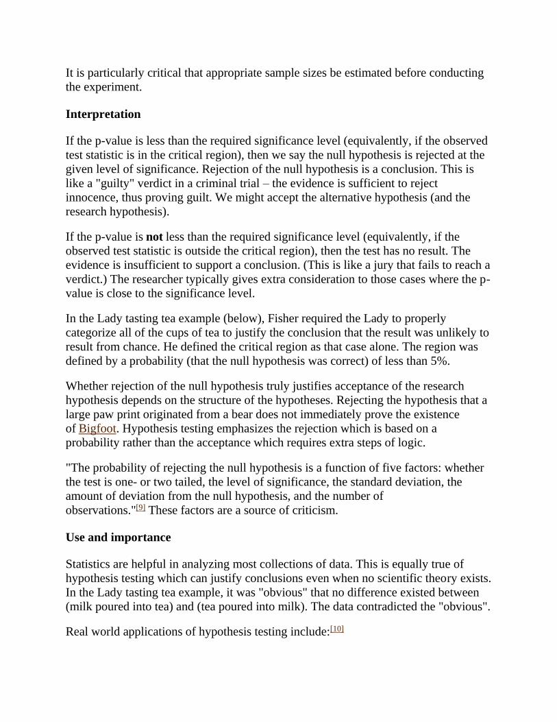
It is particularly critical that appropriate sample sizes be estimated before conducting
the experiment.
Interpretation
If the p-value is less than the required significance level (equivalently, if the observed
test statistic is in the critical region), then we say the null hypothesis is rejected at the
given level of significance. Rejection of the null hypothesis is a conclusion. This is
like a "guilty" verdict in a criminal trial – the evidence is sufficient to reject
innocence, thus proving guilt. We might accept the alternative hypothesis (and the
research hypothesis).
If the p-value is not less than the required significance level (equivalently, if the
observed test statistic is outside the critical region), then the test has no result. The
evidence is insufficient to support a conclusion. (This is like a jury that fails to reach a
verdict.) The researcher typically gives extra consideration to those cases where the p-
value is close to the significance level.
In the Lady tasting tea example (below), Fisher required the Lady to properly
categorize all of the cups of tea to justify the conclusion that the result was unlikely to
result from chance. He defined the critical region as that case alone. The region was
defined by a probability (that the null hypothesis was correct) of less than 5%.
Whether rejection of the null hypothesis truly justifies acceptance of the research
hypothesis depends on the structure of the hypotheses. Rejecting the hypothesis that a
large paw print originated from a bear does not immediately prove the existence
of Bigfoot. Hypothesis testing emphasizes the rejection which is based on a
probability rather than the acceptance which requires extra steps of logic.
"The probability of rejecting the null hypothesis is a function of five factors: whether
the test is one- or two tailed, the level of significance, the standard deviation, the
amount of deviation from the null hypothesis, and the number of
observations."[9] These factors are a source of criticism.
Use and importance
Statistics are helpful in analyzing most collections of data. This is equally true of
hypothesis testing which can justify conclusions even when no scientific theory exists.
In the Lady tasting tea example, it was "obvious" that no difference existed between
(milk poured into tea) and (tea poured into milk). The data contradicted the "obvious".
Real world applications of hypothesis testing include:[10]
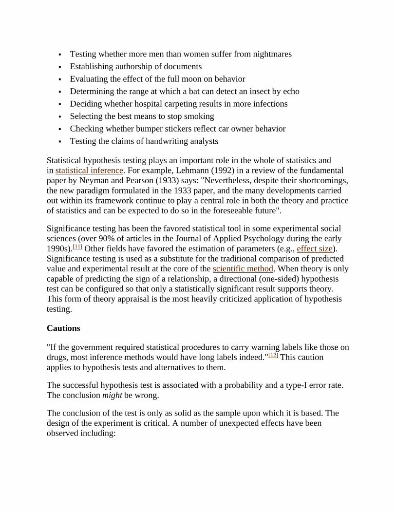
Testing whether more men than women suffer from nightmares
Establishing authorship of documents
Evaluating the effect of the full moon on behavior
Determining the range at which a bat can detect an insect by echo
Deciding whether hospital carpeting results in more infections
Selecting the best means to stop smoking
Checking whether bumper stickers reflect car owner behavior
Testing the claims of handwriting analysts
Statistical hypothesis testing plays an important role in the whole of statistics and
in statistical inference. For example, Lehmann (1992) in a review of the fundamental
paper by Neyman and Pearson (1933) says: "Nevertheless, despite their shortcomings,
the new paradigm formulated in the 1933 paper, and the many developments carried
out within its framework continue to play a central role in both the theory and practice
of statistics and can be expected to do so in the foreseeable future".
Significance testing has been the favored statistical tool in some experimental social
sciences (over 90% of articles in the Journal of Applied Psychology during the early
1990s).[11] Other fields have favored the estimation of parameters (e.g., effect size).
Significance testing is used as a substitute for the traditional comparison of predicted
value and experimental result at the core of the scientific method. When theory is only
capable of predicting the sign of a relationship, a directional (one-sided) hypothesis
test can be configured so that only a statistically significant result supports theory.
This form of theory appraisal is the most heavily criticized application of hypothesis
testing.
Cautions
"If the government required statistical procedures to carry warning labels like those on
drugs, most inference methods would have long labels indeed."[12] This caution
applies to hypothesis tests and alternatives to them.
The successful hypothesis test is associated with a probability and a type-I error rate.
The conclusion might be wrong.
The conclusion of the test is only as solid as the sample upon which it is based. The
design of the experiment is critical. A number of unexpected effects have been
observed including:
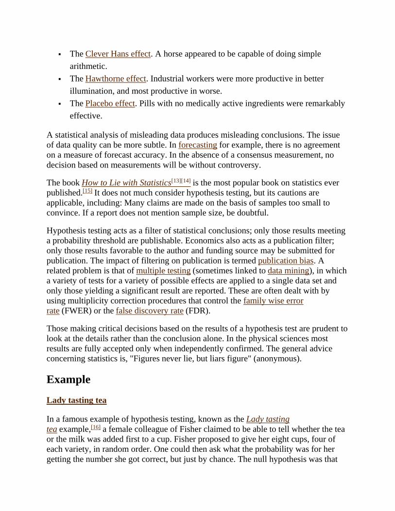
The Clever Hans effect. A horse appeared to be capable of doing simple
arithmetic.
The Hawthorne effect. Industrial workers were more productive in better
illumination, and most productive in worse.
The Placebo effect. Pills with no medically active ingredients were remarkably
effective.
A statistical analysis of misleading data produces misleading conclusions. The issue
of data quality can be more subtle. In forecasting for example, there is no agreement
on a measure of forecast accuracy. In the absence of a consensus measurement, no
decision based on measurements will be without controversy.
The book How to Lie with Statistics[13][14] is the most popular book on statistics ever
published.[15] It does not much consider hypothesis testing, but its cautions are
applicable, including: Many claims are made on the basis of samples too small to
convince. If a report does not mention sample size, be doubtful.
Hypothesis testing acts as a filter of statistical conclusions; only those results meeting
a probability threshold are publishable. Economics also acts as a publication filter;
only those results favorable to the author and funding source may be submitted for
publication. The impact of filtering on publication is termed publication bias. A
related problem is that of multiple testing (sometimes linked to data mining), in which
a variety of tests for a variety of possible effects are applied to a single data set and
only those yielding a significant result are reported. These are often dealt with by
using multiplicity correction procedures that control the family wise error
rate (FWER) or the false discovery rate (FDR).
Those making critical decisions based on the results of a hypothesis test are prudent to
look at the details rather than the conclusion alone. In the physical sciences most
results are fully accepted only when independently confirmed. The general advice
concerning statistics is, "Figures never lie, but liars figure" (anonymous).
Example
Lady tasting tea
In a famous example of hypothesis testing, known as the Lady tasting
tea example,[16] a female colleague of Fisher claimed to be able to tell whether the tea
or the milk was added first to a cup. Fisher proposed to give her eight cups, four of
each variety, in random order. One could then ask what the probability was for her
getting the number she got correct, but just by chance. The null hypothesis was that

the Lady had no such ability. The test statistic was a simple count of the number of
successes in selecting the 4 cups. The critical region was the single case of 4 successes
of 4 possible based on a conventional probability criterion (< 5%; 1 of 70 ≈ 1.4%).
Fisher asserted that no alternative hypothesis was (ever) required. The lady correctly
identified every cup,[17] which would be considered a statistically significant result.
Analogy – Courtroom trial
A statistical test procedure is comparable to a criminal trial; a defendant is considered
not guilty as long as his or her guilt is not proven. The prosecutor tries to prove the
guilt of the defendant. Only when there is enough charging evidence the defendant is
convicted.
In the start of the procedure, there are two hypotheses : "the defendant is not
guilty", and : "the defendant is guilty". The first one is called null hypothesis, and is
for the time being accepted. The second one is called alternative (hypothesis). It is the
hypothesis one hopes to support.
The hypothesis of innocence is only rejected when an error is very unlikely, because
one doesn't want to convict an innocent defendant. Such an error is called error of the
first kind (i.e., the conviction of an innocent person), and the occurrence of this error
is controlled to be rare. As a consequence of this asymmetric behaviour, the error of
the second kind (acquitting a person who committed the crime), is often rather large.
H0 is true
Truly not guilty
H1 is true
Truly guilty
Accept Null Hypothesis
Acquittal Right decision
Wrong decision
Type II Error
Reject Null Hypothesis
Conviction
Wrong decision
Type I Error Right decision
A criminal trial can be regarded as either or both of two decision processes: guilty vs
not guilty or evidence vs a threshold ("beyond a reasonable doubt"). In one view, the
defendant is judged; in the other view the performance of the prosecution (which
bears the burden of proof) is judged. A hypothesis test can be regarded as either a
judgment of a hypothesis or as a judgment of evidence.
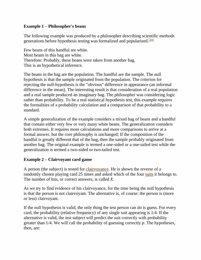
Example 1 – Philosopher's beans
The following example was produced by a philosopher describing scientific methods
generations before hypothesis testing was formalized and popularized.[18]
Few beans of this handful are white.
Most beans in this bag are white.
Therefore: Probably, these beans were taken from another bag.
This is an hypothetical inference.
The beans in the bag are the population. The handful are the sample. The null
hypothesis is that the sample originated from the population. The criterion for
rejecting the null-hypothesis is the "obvious" difference in appearance (an informal
difference in the mean). The interesting result is that consideration of a real population
and a real sample produced an imaginary bag. The philosopher was considering logic
rather than probability. To be a real statistical hypothesis test, this example requires
the formalities of a probability calculation and a comparison of that probability to a
standard.
A simple generalization of the example considers a mixed bag of beans and a handful
that contain either very few or very many white beans. The generalization considers
both extremes. It requires more calculations and more comparisons to arrive at a
formal answer, but the core philosophy is unchanged; If the composition of the
handful is greatly different that of the bag, then the sample probably originated from
another bag. The original example is termed a one-sided or a one-tailed test while the
generalization is termed a two-sided or two-tailed test.
Example 2 – Clairvoyant card game
A person (the subject) is tested for clairvoyance. He is shown the reverse of a
randomly chosen playing card 25 times and asked which of the four suits it belongs to.
The number of hits, or correct answers, is called X.
As we try to find evidence of his clairvoyance, for the time being the null hypothesis
is that the person is not clairvoyant. The alternative is, of course: the person is (more
or less) clairvoyant.
If the null hypothesis is valid, the only thing the test person can do is guess. For every
card, the probability (relative frequency) of any single suit appearing is 1/4. If the
alternative is valid, the test subject will predict the suit correctly with probability
greater than 1/4. We will call the probability of guessing correctly p. The hypotheses,
then, are:
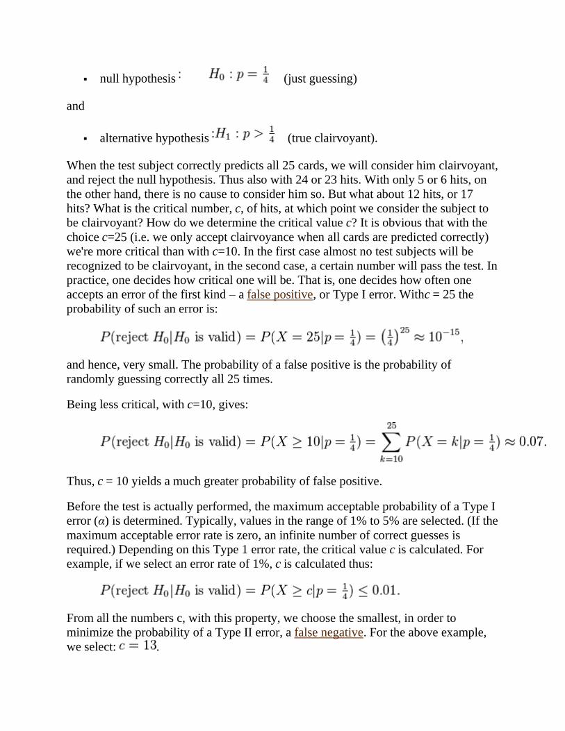
null hypothesis (just guessing)
and
alternative hypothesis (true clairvoyant).
When the test subject correctly predicts all 25 cards, we will consider him clairvoyant,
and reject the null hypothesis. Thus also with 24 or 23 hits. With only 5 or 6 hits, on
the other hand, there is no cause to consider him so. But what about 12 hits, or 17
hits? What is the critical number, c, of hits, at which point we consider the subject to
be clairvoyant? How do we determine the critical value c? It is obvious that with the
choice c=25 (i.e. we only accept clairvoyance when all cards are predicted correctly)
we're more critical than with c=10. In the first case almost no test subjects will be
recognized to be clairvoyant, in the second case, a certain number will pass the test. In
practice, one decides how critical one will be. That is, one decides how often one
accepts an error of the first kind – a false positive, or Type I error. Withc = 25 the
probability of such an error is:
and hence, very small. The probability of a false positive is the probability of
randomly guessing correctly all 25 times.
Being less critical, with c=10, gives:
Thus, c = 10 yields a much greater probability of false positive.
Before the test is actually performed, the maximum acceptable probability of a Type I
error (α) is determined. Typically, values in the range of 1% to 5% are selected. (If the
maximum acceptable error rate is zero, an infinite number of correct guesses is
required.) Depending on this Type 1 error rate, the critical value c is calculated. For
example, if we select an error rate of 1%, c is calculated thus:
From all the numbers c, with this property, we choose the smallest, in order to
minimize the probability of a Type II error, a false negative. For the above example,
we select: .
Example 3 – Radioactive suitcase
As an example, consider determining whether a suitcase contains some radioactive
material. Placed under a Geiger counter, it produces 10 counts per minute. The null
hypothesis is that no radioactive material is in the suitcase and that all measured
counts are due to ambient radioactivity typical of the surrounding air and harmless
objects. We can then calculate how likely it is that we would observe 10 counts per
minute if the null hypothesis were true. If the null hypothesis predicts (say) on
average 9 counts per minute, then according to the Poisson distribution typical
for radioactive decay there is about 41% chance of recording 10 or more counts. Thus
we can say that the suitcase is compatible with the null hypothesis (this does not
guarantee that there is no radioactive material, just that we don't have enough
evidence to suggest there is). On the other hand, if the null hypothesis predicts 3
counts per minute (for which the Poisson distribution predicts only 0.1% chance of
recording 10 or more counts) then the suitcase is not compatible with the null
hypothesis, and there are likely other factors responsible to produce the
measurements.
The test does not directly assert the presence of radioactive material. A successful test
asserts that the claim of no radioactive material present is unlikely given the reading
(and therefore ...). The double negative (disproving the null hypothesis) of the method
is confusing, but using a counter-example to disprove is standard mathematical
practice. The attraction of the method is its practicality. We know (from experience)
the expected range of counts with only ambient radioactivity present, so we can say
that a measurement is unusually large. Statistics just formalizes the intuitive by using
numbers instead of adjectives. We probably do not know the characteristics of the
radioactive suitcases; We just assume that they produce larger readings.
To slightly formalize intuition: Radioactivity is suspected if the Geiger-count with the
suitcase is among or exceeds the greatest (5% or 1%) of the Geiger-counts made with
ambient radiation alone. This makes no assumptions about the distribution of counts.
Many ambient radiation observations are required to obtain good probability estimates
for rare events.
The test described here is more fully the null-hypothesis statistical significance test.
The null hypothesis represents what we would believe by default, before seeing any
evidence. Statistical significance is a possible finding of the test, declared when the
observed sample is unlikely to have occurred by chance if the null hypothesis were
true. The name of the test describes its formulation and its possible outcome. One
characteristic of the test is its crisp decision: to reject or not reject the null hypothesis.
A calculated value is compared to a threshold, which is determined from the tolerable
risk of error.
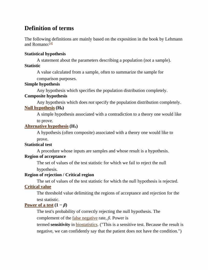
Definition of terms
The following definitions are mainly based on the exposition in the book by Lehmann
and Romano:[4]
Statistical hypothesis
A statement about the parameters describing a population (not a sample).
Statistic
A value calculated from a sample, often to summarize the sample for
comparison purposes.
Simple hypothesis
Any hypothesis which specifies the population distribution completely.
Composite hypothesis
Any hypothesis which does not specify the population distribution completely.
Null hypothesis (H0)
A simple hypothesis associated with a contradiction to a theory one would like
to prove.
Alternative hypothesis (H1)
A hypothesis (often composite) associated with a theory one would like to
prove.
Statistical test
A procedure whose inputs are samples and whose result is a hypothesis.
Region of acceptance
The set of values of the test statistic for which we fail to reject the null
hypothesis.
Region of rejection / Critical region
The set of values of the test statistic for which the null hypothesis is rejected.
Critical value
The threshold value delimiting the regions of acceptance and rejection for the
test statistic.
Power of a test (1 − β)
The test's probability of correctly rejecting the null hypothesis. The
complement of the false negative rate, β. Power is
termed sensitivity in biostatistics. ("This is a sensitive test. Because the result is
negative, we can confidently say that the patient does not have the condition.")
See sensitivity and specificity and Type I and type II errors for exhaustive
definitions.
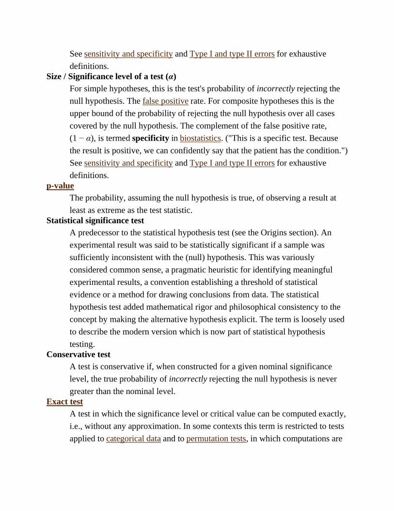
Size / Significance level of a test (α)
For simple hypotheses, this is the test's probability of incorrectly rejecting the
null hypothesis. The false positive rate. For composite hypotheses this is the
upper bound of the probability of rejecting the null hypothesis over all cases
covered by the null hypothesis. The complement of the false positive rate,
(1 − α), is termed specificity in biostatistics. ("This is a specific test. Because
the result is positive, we can confidently say that the patient has the condition.")
See sensitivity and specificity and Type I and type II errors for exhaustive
definitions.
p-value
The probability, assuming the null hypothesis is true, of observing a result at
least as extreme as the test statistic.
Statistical significance test
A predecessor to the statistical hypothesis test (see the Origins section). An
experimental result was said to be statistically significant if a sample was
sufficiently inconsistent with the (null) hypothesis. This was variously
considered common sense, a pragmatic heuristic for identifying meaningful
experimental results, a convention establishing a threshold of statistical
evidence or a method for drawing conclusions from data. The statistical
hypothesis test added mathematical rigor and philosophical consistency to the
concept by making the alternative hypothesis explicit. The term is loosely used
to describe the modern version which is now part of statistical hypothesis
testing.
Conservative test
A test is conservative if, when constructed for a given nominal significance
level, the true probability of incorrectly rejecting the null hypothesis is never
greater than the nominal level.
Exact test
A test in which the significance level or critical value can be computed exactly,
i.e., without any approximation. In some contexts this term is restricted to tests
applied to categorical data and to permutation tests, in which computations are
carried out by complete enumeration of all possible outcomes and their
probabilities.
A statistical hypothesis test compares a test statistic (z or t for examples) to a
threshold. The test statistic (the formula found in the table below) is based on
optimality. For a fixed level of Type I error rate, use of these statistics minimizes
Type II error rates (equivalent to maximizing power). The following terms describe
tests in terms of such optimality:
Most powerful test
For a given size or significance level, the test with the greatest power
(probability of rejection) for a given value of the parameter(s) being tested,
contained in the alternative hypothesis.
Uniformly most powerful test (UMP)
A test with the greatest power for all values of the parameter(s) being tested,
contained in the alternative hypothesis.
Common test statistics
Main article: Test statistic
One-sample tests are appropriate when a sample is being compared to the population
from a hypothesis. The population characteristics are known from theory or are
calculated from the population.
Two-sample tests are appropriate for comparing two samples, typically experimental
and control samples from a scientifically controlled experiment.
Paired tests are appropriate for comparing two samples where it is impossible to
control important variables. Rather than comparing two sets, members are paired
between samples so the difference between the members becomes the sample.
Typically the mean of the differences is then compared to zero.
Z-tests are appropriate for comparing means under stringent conditions regarding
normality and a known standard deviation.
T-tests are appropriate for comparing means under relaxed conditions (less is
assumed).
Tests of proportions are analogous to tests of means (the 50% proportion).
Chi-squared tests use the same calculations and the same probability distribution for
different applications:
Chi-squared tests for variance are used to determine whether a normal
population has a specified variance. The null hypothesis is that it does.
Chi-squared tests of independence are used for deciding whether two variables
are associated or are independent. The variables are categorical rather than
numeric. It can be used to decide whether left-handedness is correlated
with libertarian politics (or not). The null hypothesis is that the variables are
independent. The numbers used in the calculation are the observed and
expected frequencies of occurrence (from contingency tables).
Chi-squared goodness of fit tests are used to determine the adequacy of curves
fit to data. The null hypothesis is that the curve fit is adequate. It is common to
determine curve shapes to minimize the mean square error, so it is appropriate
that the goodness-of-fit calculation sums the squared errors.
F-tests (analysis of variance, ANOVA) are commonly used when deciding whether
groupings of data by category are meaningful. If the variance of test scores of the left-
handed in a class is much smaller than the variance of the whole class, then it may be
useful to study lefties as a group. The null hypothesis is that two variances are the
same – so the proposed grouping is not meaningful.
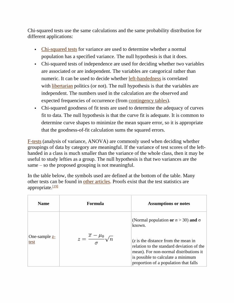
In the table below, the symbols used are defined at the bottom of the table. Many
other tests can be found in other articles. Proofs exist that the test statistics are
appropriate.[19]
Name Formula Assumptions or notes
One-sample z-
test
(Normal population or n > 30) and σ
known.
(z is the distance from the mean in
relation to the standard deviation of the
mean). For non-normal distributions it
is possible to calculate a minimum
proportion of a population that falls
within k standard deviations for
any k (see: Chebyshev's inequality).
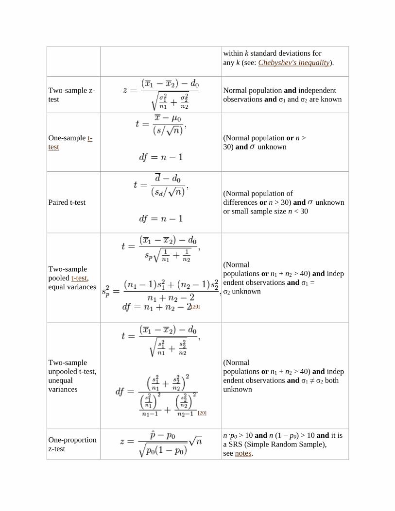
Two-sample z-
test
Normal population and independent
observations and σ1 and σ2 are known
One-sample t-
test
(Normal population or n >
30) and unknown
Paired t-test
(Normal population of
differences or n > 30) and unknown
or small sample size n < 30
Two-sample
pooled t-test,
equal variances
[20]
(Normal
populations or n1 + n2 > 40) and indep
endent observations and σ1 =
σ2 unknown
Two-sample
unpooled t-test,
unequal
variances
[20]
(Normal
populations or n1 + n2 > 40) and indep
endent observations and σ1 ≠ σ2 both
unknown
One-proportion
z-test
n .p0 > 10 and n (1 − p0) > 10 and it is
a SRS (Simple Random Sample),
see notes.
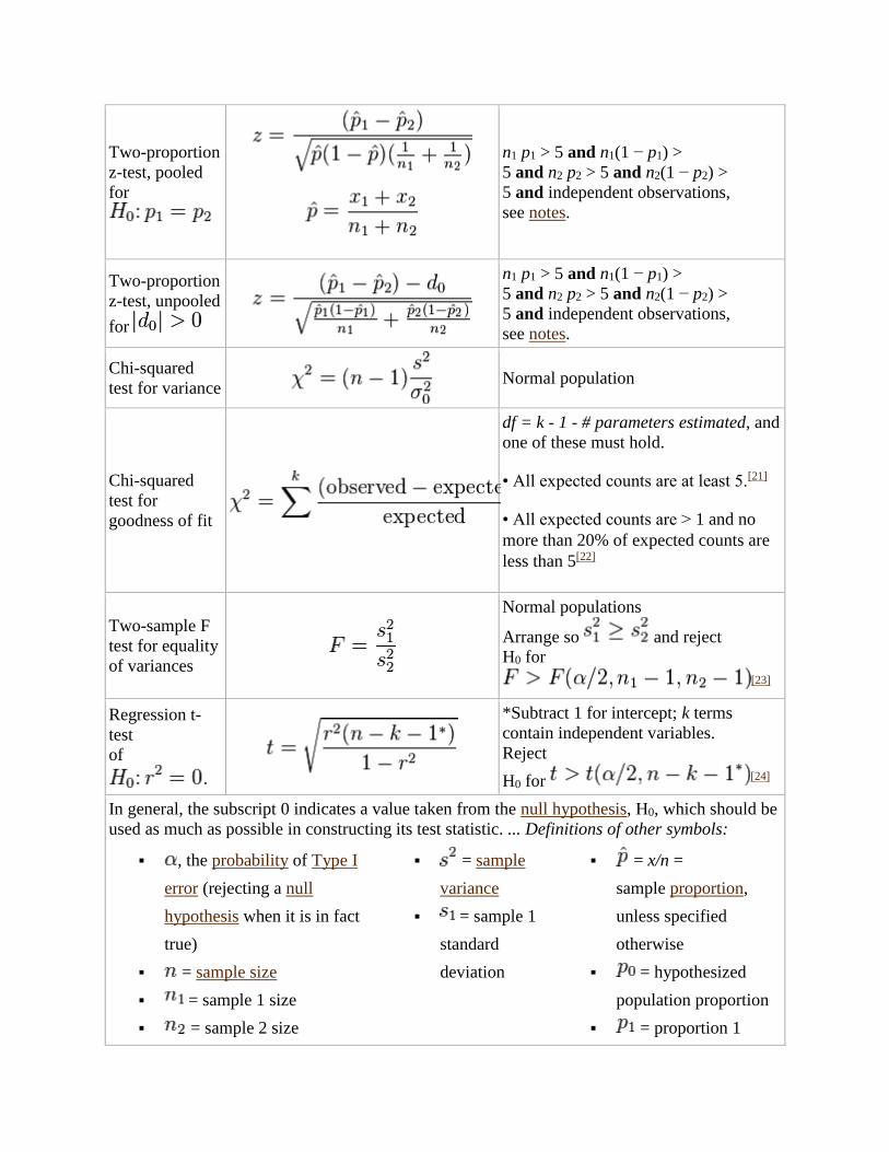
Two-proportion
z-test, pooled
for
n1 p1 > 5 and n1(1 − p1) >
5 and n2 p2 > 5 and n2(1 − p2) >
5 and independent observations,
see notes.
Two-proportion
z-test, unpooled
for
n1 p1 > 5 and n1(1 − p1) >
5 and n2 p2 > 5 and n2(1 − p2) >
5 and independent observations,
see notes.
Chi-squared
test for variance
Normal population
Chi-squared
test for
goodness of fit
df = k - 1 - # parameters estimated, and
one of these must hold.
• All expected counts are at least 5.[21]
• All expected counts are > 1 and no
more than 20% of expected counts are
less than 5[22]
Two-sample F
test for equality
of variances
Normal populations
Arrange so and reject
H0 for
[23]
Regression t-
test
of
*Subtract 1 for intercept; k terms
contain independent variables.
Reject
H0 for [24]
In general, the subscript 0 indicates a value taken from the null hypothesis, H0, which should be
used as much as possible in constructing its test statistic. ... Definitions of other symbols:
, the probability of Type I
error (rejecting a null
hypothesis when it is in fact
true)
= sample size
= sample 1 size
= sample 2 size
= sample
variance
= sample 1
standard
deviation
= x/n =
sample proportion,
unless specified
otherwise
= hypothesized
population proportion
= proportion 1
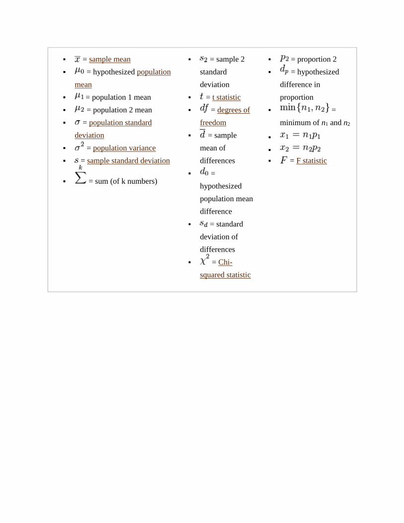
= sample mean
= hypothesized population
mean
= population 1 mean
= population 2 mean
= population standard
deviation
= population variance
= sample standard deviation
= sum (of k numbers)
= sample 2
standard
deviation
= t statistic
= degrees of
freedom
= sample
mean of
differences
=
hypothesized
population mean
difference
= standard
deviation of
differences
= Chi-
squared statistic
= proportion 2
= hypothesized
difference in
proportion
=
minimum of n1 and n2
= F statistic

Origins and early controversy
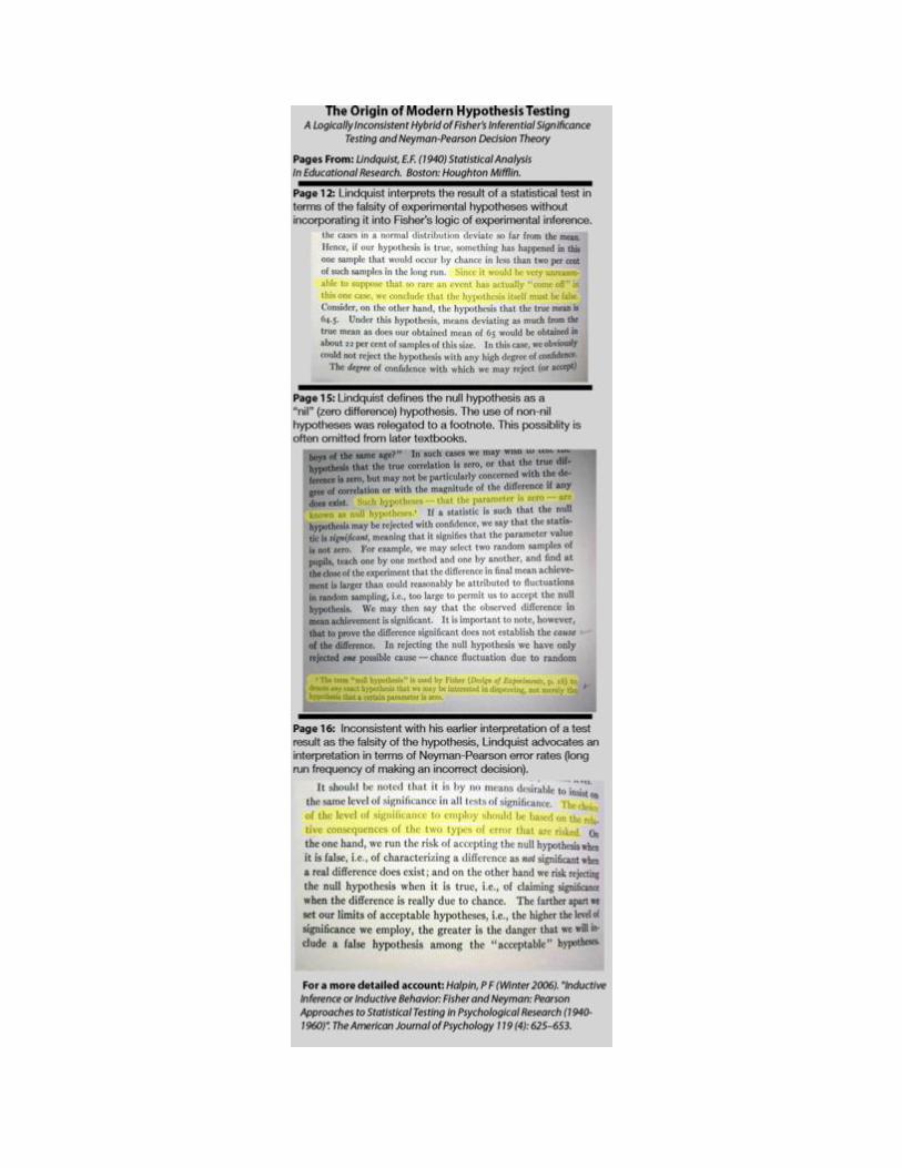
A likely originator of the "hybrid" method of hypothesis testing, as well as the use of "nil" null hypotheses,
is E.F. Lindquist in his statistics textbook: Lindquist, E.F. (1940) Statistical Analysis In Educational Research.
Boston: Houghton Mifflin.
Significance testing is largely the product of Karl Pearson (p-value, Pearson's chi-
squared test), William Sealy Gosset (Student's t-distribution), and Ronald Fisher ("null
hypothesis", analysis of variance, "significance test"), while hypothesis testing was
developed by Jerzy Neyman and Egon Pearson (son of Karl). Ronald Fisher,
mathematician and biologist described by Richard Dawkins as "the greatest biologist
since Darwin", began his life in statistics as a Bayesian (Zabell 1992), but Fisher soon
grew disenchanted with the subjectivity involved (namely use of the principle of
indifference when determining prior probabilities), and sought to provide a more
"objective" approach to inductive inference.[25]
Fisher was an agricultural statistician who emphasized rigorous experimental design
and methods to extract a result from few samples assuming Gaussian distributions.
Neyman (who teamed with the younger Pearson) emphasized mathematical rigor and
methods to obtain more results from many samples and a wider range of distributions.
Modern hypothesis testing is an inconsistent hybrid of the Fisher vs Neyman/Pearson
formulation, methods and terminology developed in the early 20th century. While
hypothesis testing was popularized early in the 20th century, evidence of its use can
be found much earlier. In the 1770s Laplace considered the statistics of almost half a
million births. The statistics showed an excess of boys compared to girls.[26] He
concluded by calculation of a p-value that the excess was a real, but unexplained,
effect.[27]
Fisher popularized the "significance test". He required a null-hypothesis
(corresponding to a population frequency distribution) and a sample. His (now
familiar) calculations determined whether to reject the null-hypothesis or not.
Significance testing did not utilize an alternative hypothesis so there was no concept
of a Type II error.
The p-value was devised as an informal, but objective, index meant to help a
researcher determine (based on other knowledge) whether to modify future
experiments or strengthen one's faith in the null hypothesis.[28] Hypothesis testing (and
Type I/II errors) was devised by Neyman and Pearson as a more objective alternative
to Fisher's p-value, also meant to determine researcher behaviour, but without
requiring any inductive inference by the researcher.[29][30]
Neyman & Pearson considered a different problem (which they called "hypothesis
testing"). They initially considered two simple hypotheses (both with frequency
distributions). They calculated two probabilities and typically selected the hypothesis
associated with the higher probability (the hypothesis more likely to have generated
the sample). Their method always selected a hypothesis. It also allowed the
calculation of both types of error probabilities.
Fisher and Neyman/Pearson clashed bitterly. Neyman/Pearson considered their
formulation to be an improved generalization of significance testing.(The defining
paper[29] was abstract. Mathematicians have generalized and refined the theory for
decades.[31]) Fisher thought that it was not applicable to scientific research because
often, during the course of the experiment, it is discovered that the initial assumptions
about the null hypothesis are questionable due to unexpected sources of error. He
believed that the use of rigid reject/accept decisions based on models formulated
before data is collected was incompatible with this common scenario faced by
scientists and attempts to apply this method to scientific research would lead to mass
confusion.[32]
The dispute between Fisher and Neyman-Pearson was waged on philosophical
grounds, characterized by a philosopher as a dispute over the proper role of models in
statistical inference.[33]
Events intervened: Neyman accepted a position in the western hemisphere, breaking
his partnership with Pearson and separating disputants (who had occupied the same
building) by much of the planetary diameter. World War II provided an intermission
in the debate. The dispute between Fisher and Neyman terminated (unresolved after
27 years) with Fisher's death in 1962. Neyman wrote a well-regarded eulogy.[34] Some
of Neyman's later publications reported p-values and significance levels.[35]
The modern version of hypothesis testing is a hybrid of the two approaches that
resulted from confusion by writers of statistical textbooks (as predicted by Fisher)
beginning in the 1940s.[36] (But signal detection, for example, still uses the
Neyman/Pearson formulation.) Great conceptual differences and many caveats in
addition to those mentioned above were ignored. Neyman and Pearson provided the
stronger terminology, the more rigorous mathematics and the more consistent
philosophy, but the subject taught today in introductory statistics has more similarities
with Fisher's method than theirs.[37] This history explains the inconsistent terminology
(example: the null hypothesis is never accepted, but there is a region of acceptance).
Sometime around 1940,[36] in an apparent effort to provide researchers with a "non-
controversial"[38] way to have their cake and eat it too, the authors of statistical text
books began anonymously combining these two strategies by using the p-value in
place of the test statistic (or data) to test against the Neyman-Pearson "significance
level".[36] Thus, researchers were encouraged to infer the strength of their data against
some null hypothesis using p-values, while also thinking they are retaining the post-
data collection objectivity provided by hypothesis testing. It then became customary
for the null hypothesis, which was originally some realistic research hypothesis, to be
used almost solely as a strawman "nil" hypothesis (one where a treatment has no
effect, regardless of the context).[39]
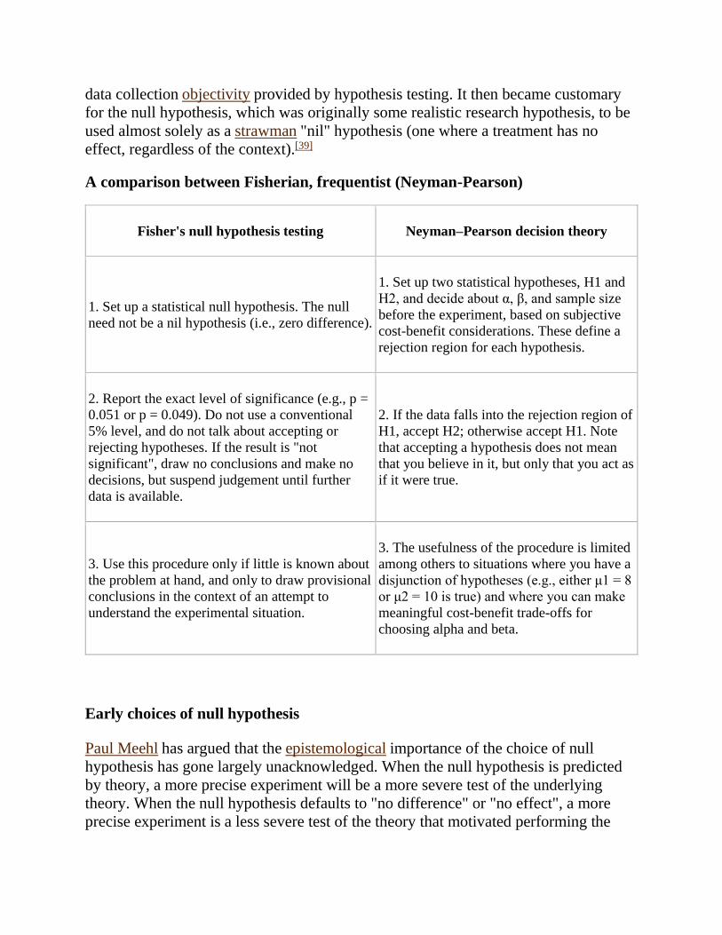
A comparison between Fisherian, frequentist (Neyman-Pearson)
Fisher's null hypothesis testing Neyman–Pearson decision theory
1. Set up a statistical null hypothesis. The null
need not be a nil hypothesis (i.e., zero difference).
1. Set up two statistical hypotheses, H1 and
H2, and decide about α, β, and sample size
before the experiment, based on subjective
cost-benefit considerations. These define a
rejection region for each hypothesis.
2. Report the exact level of significance (e.g., p =
0.051 or p = 0.049). Do not use a conventional
5% level, and do not talk about accepting or
rejecting hypotheses. If the result is "not
significant", draw no conclusions and make no
decisions, but suspend judgement until further
data is available.
2. If the data falls into the rejection region of
H1, accept H2; otherwise accept H1. Note
that accepting a hypothesis does not mean
that you believe in it, but only that you act as
if it were true.
3. Use this procedure only if little is known about
the problem at hand, and only to draw provisional
conclusions in the context of an attempt to
understand the experimental situation.
3. The usefulness of the procedure is limited
among others to situations where you have a
disjunction of hypotheses (e.g., either μ1 = 8
or μ2 = 10 is true) and where you can make
meaningful cost-benefit trade-offs for
choosing alpha and beta.
Early choices of null hypothesis
Paul Meehl has argued that the epistemological importance of the choice of null
hypothesis has gone largely unacknowledged. When the null hypothesis is predicted
by theory, a more precise experiment will be a more severe test of the underlying
theory. When the null hypothesis defaults to "no difference" or "no effect", a more
precise experiment is a less severe test of the theory that motivated performing the
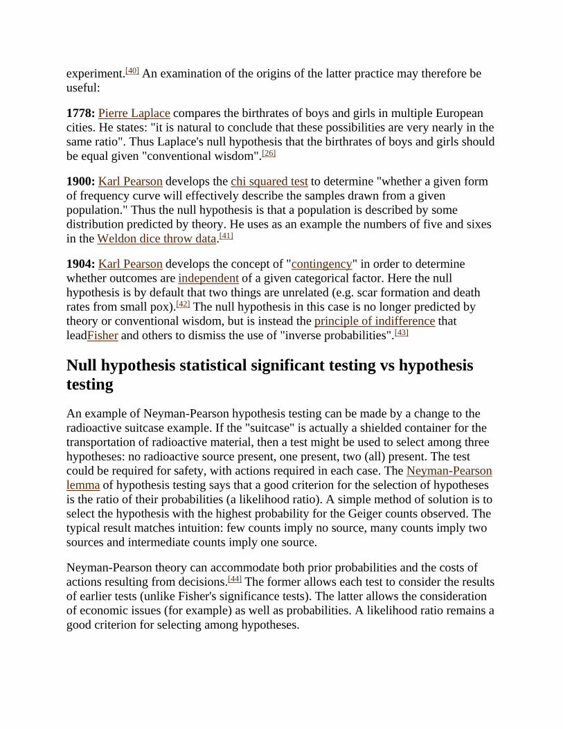
experiment.[40] An examination of the origins of the latter practice may therefore be
useful:
1778: Pierre Laplace compares the birthrates of boys and girls in multiple European
cities. He states: "it is natural to conclude that these possibilities are very nearly in the
same ratio". Thus Laplace's null hypothesis that the birthrates of boys and girls should
be equal given "conventional wisdom".[26]
1900: Karl Pearson develops the chi squared test to determine "whether a given form
of frequency curve will effectively describe the samples drawn from a given
population." Thus the null hypothesis is that a population is described by some
distribution predicted by theory. He uses as an example the numbers of five and sixes
in the Weldon dice throw data.[41]
1904: Karl Pearson develops the concept of "contingency" in order to determine
whether outcomes are independent of a given categorical factor. Here the null
hypothesis is by default that two things are unrelated (e.g. scar formation and death
rates from small pox).[42] The null hypothesis in this case is no longer predicted by
theory or conventional wisdom, but is instead the principle of indifference that
leadFisher and others to dismiss the use of "inverse probabilities".[43]
Null hypothesis statistical significant testing vs hypothesis
testing
An example of Neyman-Pearson hypothesis testing can be made by a change to the
radioactive suitcase example. If the "suitcase" is actually a shielded container for the
transportation of radioactive material, then a test might be used to select among three
hypotheses: no radioactive source present, one present, two (all) present. The test
could be required for safety, with actions required in each case. The Neyman-Pearson
lemma of hypothesis testing says that a good criterion for the selection of hypotheses
is the ratio of their probabilities (a likelihood ratio). A simple method of solution is to
select the hypothesis with the highest probability for the Geiger counts observed. The
typical result matches intuition: few counts imply no source, many counts imply two
sources and intermediate counts imply one source.
Neyman-Pearson theory can accommodate both prior probabilities and the costs of
actions resulting from decisions.[44] The former allows each test to consider the results
of earlier tests (unlike Fisher's significance tests). The latter allows the consideration
of economic issues (for example) as well as probabilities. A likelihood ratio remains a
good criterion for selecting among hypotheses.
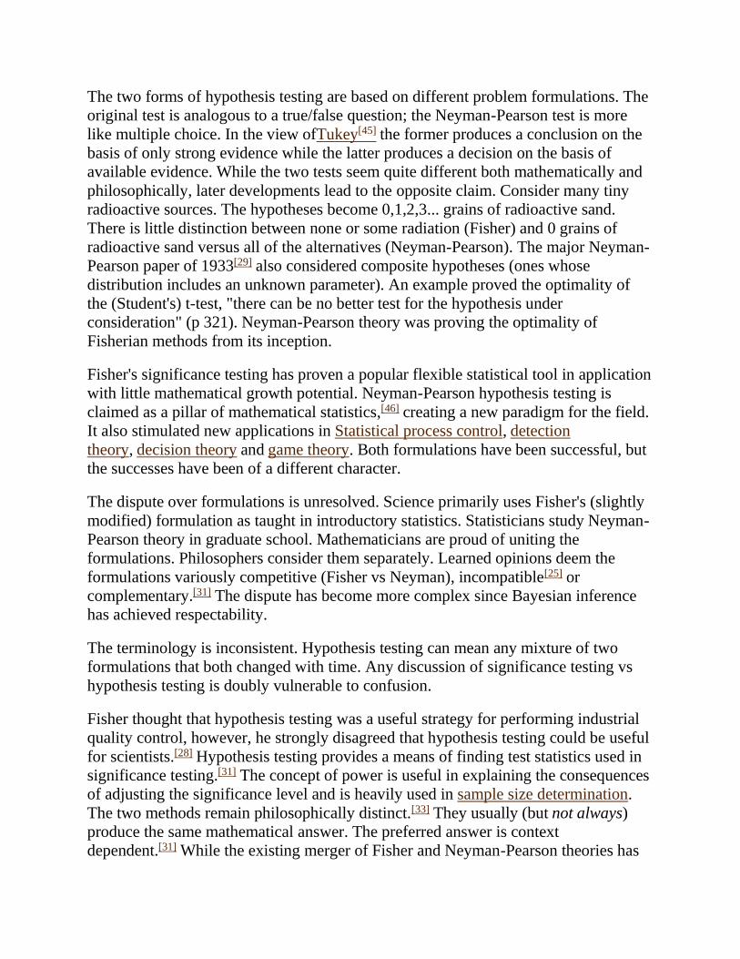
The two forms of hypothesis testing are based on different problem formulations. The
original test is analogous to a true/false question; the Neyman-Pearson test is more
like multiple choice. In the view ofTukey[45] the former produces a conclusion on the
basis of only strong evidence while the latter produces a decision on the basis of
available evidence. While the two tests seem quite different both mathematically and
philosophically, later developments lead to the opposite claim. Consider many tiny
radioactive sources. The hypotheses become 0,1,2,3... grains of radioactive sand.
There is little distinction between none or some radiation (Fisher) and 0 grains of
radioactive sand versus all of the alternatives (Neyman-Pearson). The major Neyman-
Pearson paper of 1933[29] also considered composite hypotheses (ones whose
distribution includes an unknown parameter). An example proved the optimality of
the (Student's) t-test, "there can be no better test for the hypothesis under
consideration" (p 321). Neyman-Pearson theory was proving the optimality of
Fisherian methods from its inception.
Fisher's significance testing has proven a popular flexible statistical tool in application
with little mathematical growth potential. Neyman-Pearson hypothesis testing is
claimed as a pillar of mathematical statistics,[46] creating a new paradigm for the field.
It also stimulated new applications in Statistical process control, detection
theory, decision theory and game theory. Both formulations have been successful, but
the successes have been of a different character.
The dispute over formulations is unresolved. Science primarily uses Fisher's (slightly
modified) formulation as taught in introductory statistics. Statisticians study Neyman-
Pearson theory in graduate school. Mathematicians are proud of uniting the
formulations. Philosophers consider them separately. Learned opinions deem the
formulations variously competitive (Fisher vs Neyman), incompatible[25] or
complementary.[31] The dispute has become more complex since Bayesian inference
has achieved respectability.
The terminology is inconsistent. Hypothesis testing can mean any mixture of two
formulations that both changed with time. Any discussion of significance testing vs
hypothesis testing is doubly vulnerable to confusion.
Fisher thought that hypothesis testing was a useful strategy for performing industrial
quality control, however, he strongly disagreed that hypothesis testing could be useful
for scientists.[28] Hypothesis testing provides a means of finding test statistics used in
significance testing.[31] The concept of power is useful in explaining the consequences
of adjusting the significance level and is heavily used in sample size determination.
The two methods remain philosophically distinct.[33] They usually (but not always)
produce the same mathematical answer. The preferred answer is context
dependent.[31] While the existing merger of Fisher and Neyman-Pearson theories has

been heavily criticized, modifying the merger to achieve Bayesian goals has been
considered.[47]
Criticism
Criticism of statistical hypothesis testing fills volumes[48][49][50][51][52][53] citing 300–400
primary references. Much of the criticism can be summarized by the following issues:
The interpretation of a p-value is dependent upon stopping rule and definition
of multiple comparison. The former often changes during the course of a study
and the latter is unavoidably ambiguous. (i.e. "p values depend on both the
(data) observed and on the other possible (data) that might have been observed
but weren't").[54]
Confusion resulting (in part) from combining the methods of Fisher and
Neyman-Pearson which are conceptually distinct.[45]
Emphasis on statistical significance to the exclusion of estimation and
confirmation by repeated experiments.[55]
Rigidly requiring statistical significance as a criterion for publication, resulting
in publication bias.[56] Most of the criticism is indirect. Rather than being
wrong, statistical hypothesis testing is misunderstood, overused and misused.
When used to detect whether a difference exists between groups, a paradox
arises. As improvements are made to experimental design (e.g., increased
precision of measurement and sample size), the test becomes more lenient.
Unless one accepts the absurd assumption that all sources of noise in the data
cancel out completely, the chance of finding statistical significance in either
direction approaches 100%.[57]
Layers of philosophical concerns. The probability of statistical significance is a
function of decisions made by experimenters/analysts.[9] If the decisions are
based on convention they are termed arbitrary or mindless[38] while those not so
based may be termed subjective. To minimize type II errors, large samples are
recommended. In psychology practically all null hypotheses are claimed to be
false for sufficiently large samples so "...it is usually nonsensical to perform an
experiment with the sole aim of rejecting the null hypothesis.".[58] "Statistically
significant findings are often misleading" in psychology.[59] Statistical
significance does not imply practical significance and correlation does not
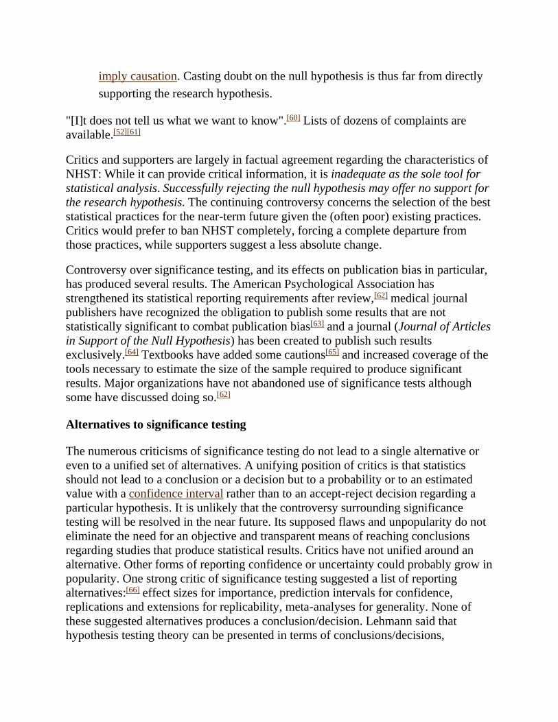
imply causation. Casting doubt on the null hypothesis is thus far from directly
supporting the research hypothesis.
"[I]t does not tell us what we want to know".[60] Lists of dozens of complaints are
available.[52][61]
Critics and supporters are largely in factual agreement regarding the characteristics of
NHST: While it can provide critical information, it is inadequate as the sole tool for
statistical analysis. Successfully rejecting the null hypothesis may offer no support for
the research hypothesis. The continuing controversy concerns the selection of the best
statistical practices for the near-term future given the (often poor) existing practices.
Critics would prefer to ban NHST completely, forcing a complete departure from
those practices, while supporters suggest a less absolute change.
Controversy over significance testing, and its effects on publication bias in particular,
has produced several results. The American Psychological Association has
strengthened its statistical reporting requirements after review,[62] medical journal
publishers have recognized the obligation to publish some results that are not
statistically significant to combat publication bias[63] and a journal (Journal of Articles
in Support of the Null Hypothesis) has been created to publish such results
exclusively.[64] Textbooks have added some cautions[65] and increased coverage of the
tools necessary to estimate the size of the sample required to produce significant
results. Major organizations have not abandoned use of significance tests although
some have discussed doing so.[62]
Alternatives to significance testing
The numerous criticisms of significance testing do not lead to a single alternative or
even to a unified set of alternatives. A unifying position of critics is that statistics
should not lead to a conclusion or a decision but to a probability or to an estimated
value with a confidence interval rather than to an accept-reject decision regarding a
particular hypothesis. It is unlikely that the controversy surrounding significance
testing will be resolved in the near future. Its supposed flaws and unpopularity do not
eliminate the need for an objective and transparent means of reaching conclusions
regarding studies that produce statistical results. Critics have not unified around an
alternative. Other forms of reporting confidence or uncertainty could probably grow in
popularity. One strong critic of significance testing suggested a list of reporting
alternatives:[66] effect sizes for importance, prediction intervals for confidence,
replications and extensions for replicability, meta-analyses for generality. None of
these suggested alternatives produces a conclusion/decision. Lehmann said that
hypothesis testing theory can be presented in terms of conclusions/decisions,
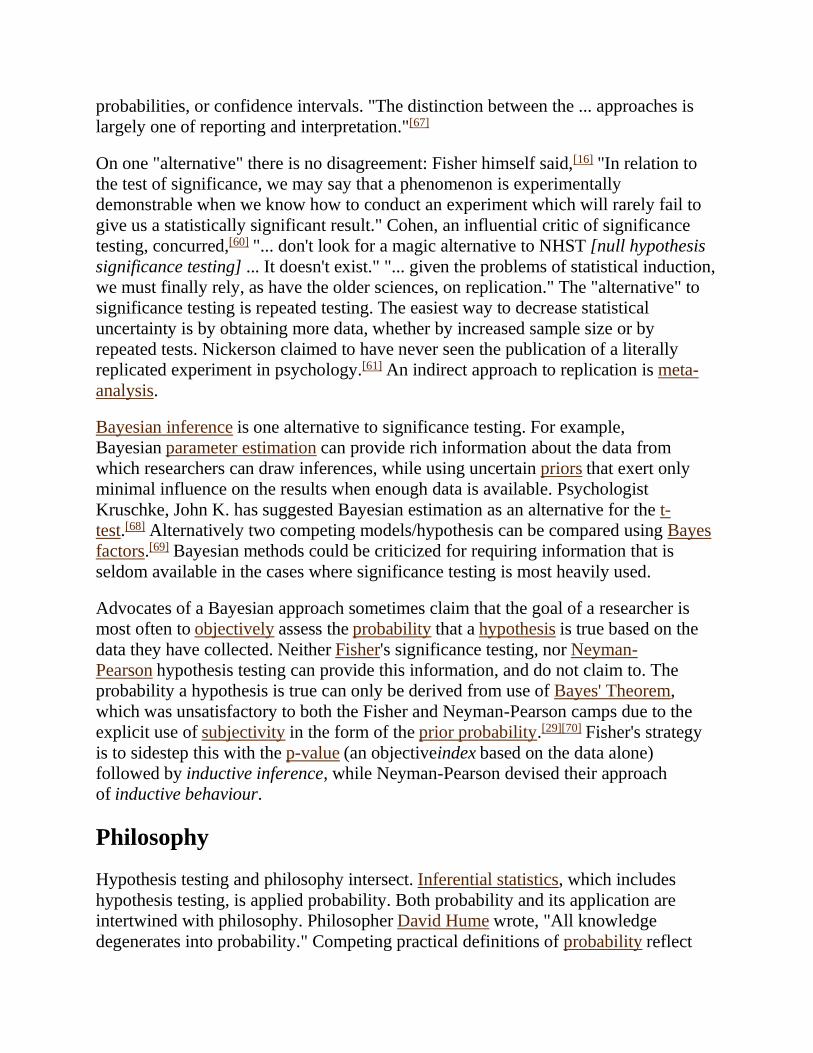
probabilities, or confidence intervals. "The distinction between the ... approaches is
largely one of reporting and interpretation."[67]
On one "alternative" there is no disagreement: Fisher himself said,[16] "In relation to
the test of significance, we may say that a phenomenon is experimentally
demonstrable when we know how to conduct an experiment which will rarely fail to
give us a statistically significant result." Cohen, an influential critic of significance
testing, concurred,[60] "... don't look for a magic alternative to NHST [null hypothesis
significance testing] ... It doesn't exist." "... given the problems of statistical induction,
we must finally rely, as have the older sciences, on replication." The "alternative" to
significance testing is repeated testing. The easiest way to decrease statistical
uncertainty is by obtaining more data, whether by increased sample size or by
repeated tests. Nickerson claimed to have never seen the publication of a literally
replicated experiment in psychology.[61] An indirect approach to replication is meta-
analysis.
Bayesian inference is one alternative to significance testing. For example,
Bayesian parameter estimation can provide rich information about the data from
which researchers can draw inferences, while using uncertain priors that exert only
minimal influence on the results when enough data is available. Psychologist
Kruschke, John K. has suggested Bayesian estimation as an alternative for the t-
test.[68] Alternatively two competing models/hypothesis can be compared using Bayes
factors.[69] Bayesian methods could be criticized for requiring information that is
seldom available in the cases where significance testing is most heavily used.
Advocates of a Bayesian approach sometimes claim that the goal of a researcher is
most often to objectively assess the probability that a hypothesis is true based on the
data they have collected. Neither Fisher's significance testing, nor Neyman-
Pearson hypothesis testing can provide this information, and do not claim to. The
probability a hypothesis is true can only be derived from use of Bayes' Theorem,
which was unsatisfactory to both the Fisher and Neyman-Pearson camps due to the
explicit use of subjectivity in the form of the prior probability.[29][70] Fisher's strategy
is to sidestep this with the p-value (an objectiveindex based on the data alone)
followed by inductive inference, while Neyman-Pearson devised their approach
of inductive behaviour.
Philosophy
Hypothesis testing and philosophy intersect. Inferential statistics, which includes
hypothesis testing, is applied probability. Both probability and its application are
intertwined with philosophy. Philosopher David Hume wrote, "All knowledge
degenerates into probability." Competing practical definitions of probability reflect
philosophical differences. The most common application of hypothesis testing is in
the scientific interpretation of experimental data, which is naturally studied by
the philosophy of science.
Fisher and Neyman opposed the subjectivity of probability. Their views contributed to
the objective definitions. The core of their historical disagreement was philosophical.
Many of the philosophical criticisms of hypothesis testing are discussed by
statisticians in other contexts, particularly correlation does not imply causation and
the design of experiments. Hypothesis testing is of continuing interest to
philosophers.[33][71]
Education
Main article: Statistics education
Statistics is increasingly being taught in schools with hypothesis testing being one of
the elements taught.[72][73] Many conclusions reported in the popular press (political
opinion polls to medical studies) are based on statistics. An informed public should
understand the limitations of statistical conclusions[74][75] and many college fields of
study require a course in statistics for the same reason.[74][75] An introductory college
statistics class places much emphasis on hypothesis testing – perhaps half of the
course. Such fields as literature and divinity now include findings based on statistical
analysis (see the Bible Analyzer). An introductory statistics class teaches hypothesis
testing as a cookbook process. Hypothesis testing is also taught at the postgraduate
level. Statisticians learn how to create good statistical test procedures (like z,
Student's t, F and chi-squared). Statistical hypothesis testing is considered a mature
area within statistics,[67] but a limited amount of development continues.
The cookbook method of teaching introductory statistics leaves no time for history,
philosophy or controversy. Hypothesis testing has been taught as received unified
method. Surveys showed that graduates of the class were filled with philosophical
misconceptions (on all aspects of statistical inference) that persisted among
instructors.[76] While the problem was addressed more than a decade ago,[77] and calls
for educational reform continue,[78] students still graduate from statistics classes
holding fundamental misconceptions about hypothesis testing.[79] Ideas for improving
the teaching of hypothesis testing include encouraging students to search for statistical
errors in published papers, teaching the history of statistics and emphasizing the
controversy in a generally dry subject.[80]