Embed Size (px)
Citation preview

Statistical Analysis of k-Nearest Neighbor
Collaborative Recommendation
Gerard BIAU a,∗, Benoıt CADRE b and Laurent ROUVIERE c
a LSTA & LPMAUniversite Pierre et Marie Curie – Paris VI
Boıte 158, 175 rue du Chevaleret75013 Paris, France
b IRMAR, ENS Cachan Bretagne, CNRS, UEBCampus de Ker Lann
Avenue Robert Schuman35170 Bruz, France
c CREST-ENSAI, IRMAR, UEBCampus de Ker Lann
Rue Blaise Pascal - BP 3720335172 Bruz Cedex, France
Abstract
Collaborative recommendation is an information-filtering techniquethat attempts to present information items that are likely of interestto an Internet user. Traditionally, collaborative systems deal withsituations with two types of variables, users and items. In its mostcommon form, the problem is framed as trying to estimate ratingsfor items that have not yet been consumed by a user. Despite wide-ranging literature, little is known about the statistical properties ofrecommendation systems. In fact, no clear probabilistic model evenexists which would allow us to precisely describe the mathematicalforces driving collaborative filtering. To provide an initial contributionto this, we propose to set out a general sequential stochastic model forcollaborative recommendation. We offer an in-depth analysis of theso-called cosine-type nearest neighbor collaborative method, which isone of the most widely used algorithms in collaborative filtering, and
∗Corresponding author.
1
analyze its asymptotic performance as the number of users grows. Weestablish consistency of the procedure under mild assumptions on themodel. Rates of convergence and examples are also provided.
Index Terms — Collaborative recommendation – cosine-type similar-ity – nearest neighbor estimate – consistency – rate of convergence.
AMS 2000 Classification: 62G05, 62G20.
1 Introduction
Collaborative recommendation is a Web information-filtering technique thattypically gathers information about your personal interests and comparesyour profile to other users with similar tastes. The goal of this system is togive personalized recommendations, whether this be movies you might enjoy,books you should read or the next restaurant you should go to.
There has been much work done in this area over the past decade since theappearance of the first papers on the subject in the mid-90’s (Resnick et al.[13], Hill et al. [11], Shardanand and Maes [16]). Stimulated by an abundanceof practical applications, most of the research activity to date has focusedon elaborating various heuristics and practical methods (Breese et al. [4],Heckerman et al. [10], Salakhutdinov et al. [14]) so as to provide personal-ized recommendations and help Web users deal with information overload.Examples of such applications include recommending books, people, restau-rants, movies, CDs and news. Websites such as amazon.com, match.com,movielens.org and allmusic.com already have recommendation systems inoperation. We refer the reader to the surveys by Adomavicius and Tuzhilin[3] and Adomavicius et al. [2] for a broader picture of the field, an overviewof results and many related references.
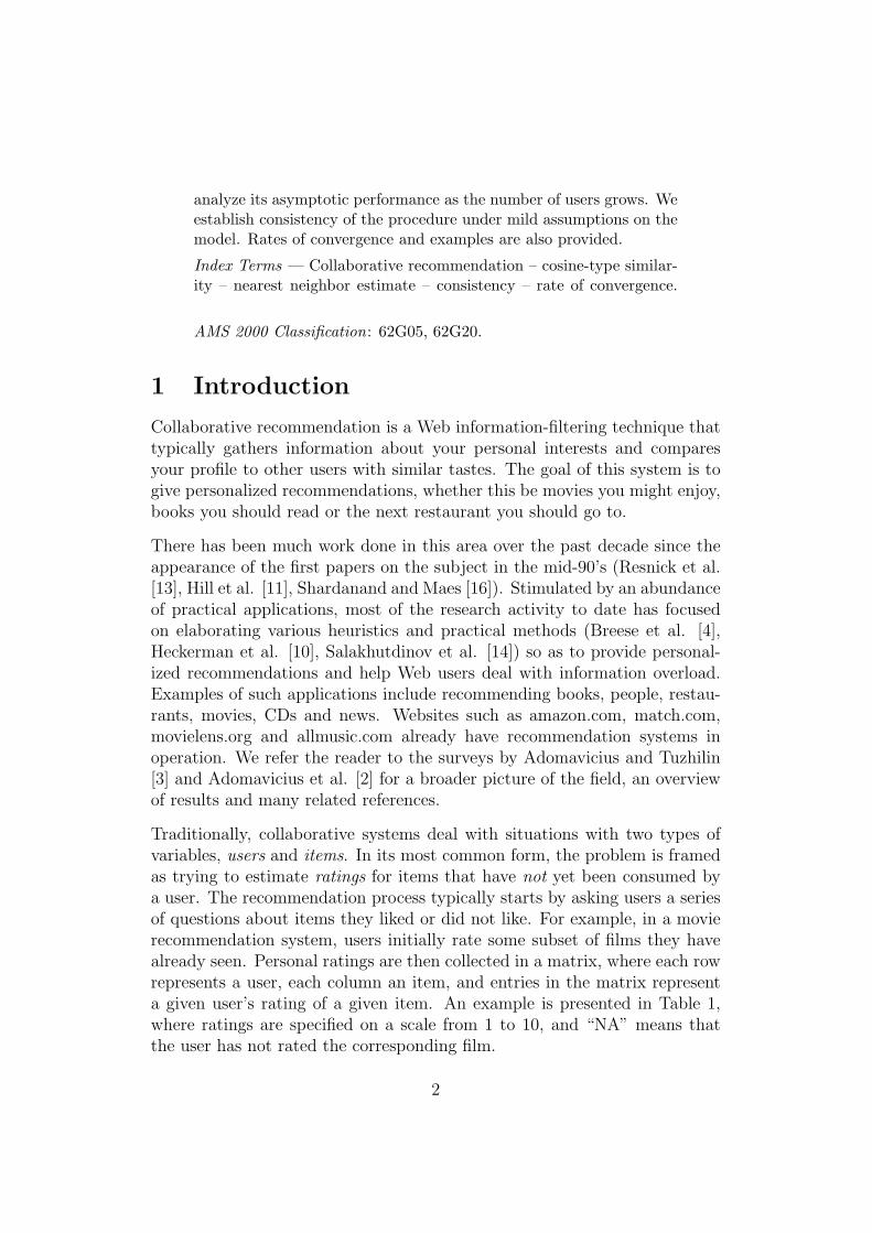
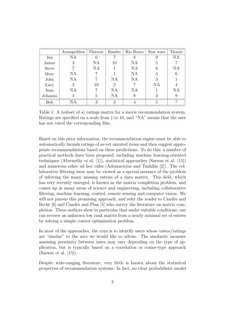
Traditionally, collaborative systems deal with situations with two types ofvariables, users and items. In its most common form, the problem is framedas trying to estimate ratings for items that have not yet been consumed bya user. The recommendation process typically starts by asking users a seriesof questions about items they liked or did not like. For example, in a movierecommendation system, users initially rate some subset of films they havealready seen. Personal ratings are then collected in a matrix, where each rowrepresents a user, each column an item, and entries in the matrix representa given user’s rating of a given item. An example is presented in Table 1,where ratings are specified on a scale from 1 to 10, and “NA” means thatthe user has not rated the corresponding film.
2
Armageddon Platoon Rambo Rio Bravo Star wars TitanicJim NA 6 7 8 9 NA
James 3 NA 10 NA 5 7Steve 7 NA 1 NA 6 NAMary NA 7 1 NA 5 6John NA 7 NA NA 3 1Lucy 3 10 2 7 NA 4Stan NA 7 NA NA 1 NA
Johanna 4 5 NA 8 3 9
Bob NA 3 3 4 5 ?
Table 1: A (subset of a) ratings matrix for a movie recommendation system.Ratings are specified on a scale from 1 to 10, and “NA” means that the userhas not rated the corresponding film.
Based on this prior information, the recommendation engine must be able toautomatically furnish ratings of as-yet unrated items and then suggest appro-priate recommendations based on these predictions. To do this, a number ofpractical methods have been proposed, including machine learning-orientedtechniques (Abernethy et al. [1]), statistical approaches (Sarwar et al. [15])and numerous other ad hoc rules (Adomavicius and Tuzhilin [2]). The col-laborative filtering issue may be viewed as a special instance of the problemof inferring the many missing entries of a data matrix. This field, whichhas very recently emerged, is known as the matrix completion problem, andcomes up in many areas of science and engineering, including collaborativefiltering, machine learning, control, remote sensing and computer vision. Wewill not pursue this promising approach, and refer the reader to Candes andRecht [6] and Candes and Plan [5] who survey the literature on matrix com-pletion. These authors show in particular that under suitable conditions, onecan recover an unknown low rank matrix from a nearly minimal set of entriesby solving a simple convex optimization problem.
In most of the approaches, the crux is to identify users whose tastes/ratingsare “similar” to the user we would like to advise. The similarity measureassessing proximity between users may vary depending on the type of ap-plication, but is typically based on a correlation or cosine-type approach(Sarwar et al. [15]).
Despite wide-ranging literature, very little is known about the statisticalproperties of recommendation systems. In fact, no clear probabilistic model
3
even exists allowing us to precisely describe the mathematical forces drivingcollaborative filtering. To provide an initial contribution to this, we proposein the present paper to set out a general stochastic model for collaborativerecommendation and analyze its asymptotic performance as the number ofusers grows.
The document is organized as follows. In section 2, we provide a sequentialstochastic model for collaborative recommendation and describe the statis-tical problem. In the model we analyze, unrated items are estimated byaveraging ratings of users who are “similar” to the user we would like to ad-vise. The similarity is assessed by a cosine-type measure, and unrated itemsare estimated using a kn-nearest neighbor-type regression estimate, whichis indeed one of the most widely used procedures in collaborative filtering.It turns out that the choice of the cosine proximity as a similarity measureimposes constraints on the model, which are discussed in section 3. Undermild assumptions, consistency of the estimation procedure is established insection 4, whereas rates of convergence are discussed in section 5. Illustrativeexamples are given throughout the document, and proofs of some technicalresults are postponed to section 6.
2 A model for collaborative recommendation
2.1 Ratings matrix and new users
Suppose that there are d + 1 (d ≥ 1) possible items, n users in the ratingsmatrix (i.e., the database) and that users’ ratings take values in the set({0} ∪ [1, s])d+1. Here, s is a real number greater than 1 corresponding tothe maximal rating and, by convention, the symbol 0 means that the userhas not rated the item (same as “NA”). Thus, the ratings matrix has n rows,d + 1 columns and entries from {0} ∪ [1, s]. For example, n = 8, d = 5 ands = 10 in Table 1, which will be our toy example throughout this section.Then, a new user Bob reveals some of his preferences for the first time, ratingsome of the first d items but not the (d + 1)th (the movie Titanic in Table1). We want to design a strategy to predict Bob’s rating of Titanic using:(i) Bob’s ratings of some (or all) of the other d movies and (ii) the ratingsmatrix. This is illustrated in Table 1, where Bob has rated 4 out of the 5movies.
The first step in our approach is to model the preferences of new user Bobby a random vector (X, Y ) of size d+1 taking values in the set [1, s]d× [1, s].Within this framework, the random variable X = (X1, . . . , Xd) represents
4
Bob’s preferences pertaining to the first d movies, whereas Y , the (unob-served) variable of interest, refers to the movie Titanic. In fact, as Bob doesnot necessarily reveals all his preferences at once, we do not observe the vari-able X, but instead some “masked” version of it denoted hereafter by X?.The random variable X? = (X?
1 , . . . , X?d) is naturally defined by
X?j =
{Xj if j ∈M0 otherwise,
where M stands for some non-empty random subset of {1, . . . , d} indexingthe movies which have been rated by Bob. Observe that the random variableX? takes values in ({0} ∪ [1, s])d and that ‖X?‖ ≥ 1, where ‖.‖ denotes theusual Euclidean norm on Rd. In the example of Table 1, M = {2, 3, 4, 5} and(the realization of) X? is (0, 3, 3, 4, 5).
We follow the same approach to model preferences of users already in thedatabase (Jim, James, Steve, Mary, etc. in Table 1), who will thereforebe represented by a sequence of independent [1, s]d × [1, s]-valued randompairs (X1, Y1), . . . , (Xn, Yn) from the distribution (X, Y ). A first idea fordealing with potential non-responses of a user i in the ratings matrix (i =1, . . . , n) is to consider in place of Xi = (Xi1, . . . , Xid) its masked version
Xi = (Xi1, . . . , Xid) defined by
Xij =
{Xij if j ∈Mi ∩M0 otherwise,
(2.1)
where each Mi is the random subset of {1, . . . , d} indexing the movies whichhave been rated by user i. In other words, we only keep in Xi items coratedby both user i and the new user — items which have not been rated by Xand Xi are declared non-informative and simply thrown away.
However, this model, which is static in nature, does not allow to take intoaccount the fact that, as time goes by, each user in the database may revealmore and more preferences. This will for instance typically be the case inthe movie recommendation system of Table 1, where regular customers willupdate their ratings each time they have seen a new movie. Consequently,model (2.1) is not fully satisfying and must therefore be slightly modified tobetter capture the sequential evolution of ratings.
2.2 A sequential model
A possible dynamical approach for collaborative recommendation is basedon the following protocol: users enter the database one after the other and
5
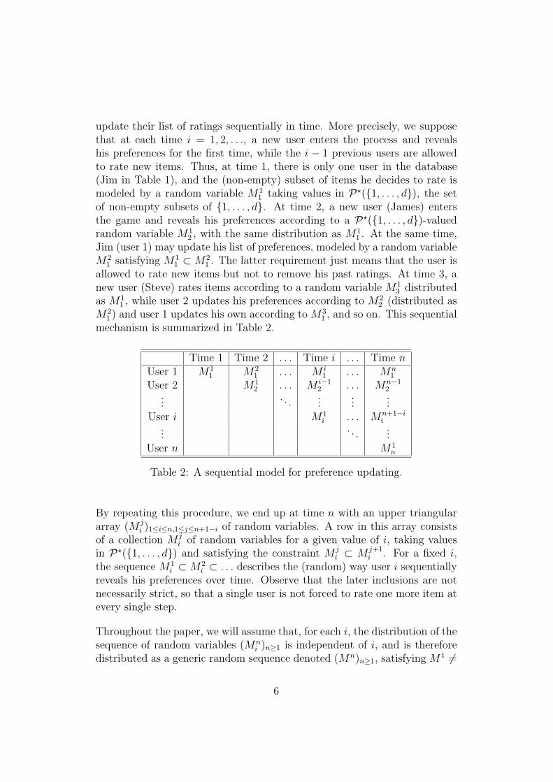
update their list of ratings sequentially in time. More precisely, we supposethat at each time i = 1, 2, . . ., a new user enters the process and revealshis preferences for the first time, while the i − 1 previous users are allowedto rate new items. Thus, at time 1, there is only one user in the database(Jim in Table 1), and the (non-empty) subset of items he decides to rate ismodeled by a random variable M1
1 taking values in P?({1, . . . , d}), the setof non-empty subsets of {1, . . . , d}. At time 2, a new user (James) entersthe game and reveals his preferences according to a P?({1, . . . , d})-valuedrandom variable M1
2 , with the same distribution as M11 . At the same time,
Jim (user 1) may update his list of preferences, modeled by a random variableM2
1 satisfying M11 ⊂M2
1 . The latter requirement just means that the user isallowed to rate new items but not to remove his past ratings. At time 3, anew user (Steve) rates items according to a random variable M1
3 distributedas M1
1 , while user 2 updates his preferences according to M22 (distributed as
M21 ) and user 1 updates his own according to M3
1 , and so on. This sequentialmechanism is summarized in Table 2.
Time 1 Time 2 . . . Time i . . . Time nUser 1 M1
1 M21 . . . M i
1 . . . Mn1
User 2 M12 . . . M i−1
2 . . . Mn−12
.... . .
......
...User i M1
i . . . Mn+1−ii
.... . .
...User n M1
n
Table 2: A sequential model for preference updating.
By repeating this procedure, we end up at time n with an upper triangulararray (M j
i )1≤i≤n,1≤j≤n+1−i of random variables. A row in this array consistsof a collection M j
i of random variables for a given value of i, taking valuesin P?({1, . . . , d}) and satisfying the constraint M j
i ⊂ M j+1i . For a fixed i,
the sequence M1i ⊂M2
i ⊂ . . . describes the (random) way user i sequentiallyreveals his preferences over time. Observe that the later inclusions are notnecessarily strict, so that a single user is not forced to rate one more item atevery single step.
Throughout the paper, we will assume that, for each i, the distribution of thesequence of random variables (Mn
i )n≥1 is independent of i, and is thereforedistributed as a generic random sequence denoted (Mn)n≥1, satisfying M1 6=
6
∅ and Mn ⊂ Mn+1 for all n ≥ 1. For the sake of coherence, we assume thatM1 and M (see (2.1)) have the same distribution, i.e., the new abstract userX? may be regarded as a user entering the database for the first time. Wewill also suppose that there exists a positive random integer n0 such thatMn0 = {1, . . . , d} and, consequently, Mn = {1, . . . , d} for all n ≥ n0. Thisrequirement means that each user rates all d items after a (random) period oftime. Last, we will assume that the pairs (Xi, Yi), i = 1, . . . , n, the sequences(Mn
1 )n≥1, (Mn2 )n≥1, . . . and the random variable M are mutually independent.
We note that this implies that the users’ ratings are independent.
With this sequential point of view, improving on (2.1), we let the masked
version X(n)i = (X
(n)i1 , . . . , X
(n)id ) of Xi be defined as
X(n)ij =
{Xij if j ∈Mn+1−i
i ∩M0 otherwise.
Again, it is worth pointing out that, in the definition of X(n)i , items which
have not been corated by both X and Xi are deleted. This implies in par-ticular that X
(n)i may be equal to 0, the d-dimensional null vector (whereas
‖X?‖ ≥ 1 by construction).
Finally, in order to deal with possible non-answers of database users regardingthe variable of interest (Titanic in our movie example), we introduce (Rn)n≥1,a sequence of random variables taking values in P?({1, . . . , n}), such thatRn is independent of M and the sequences (Mn
i )n≥1, and satisfying Rn ⊂Rn+1 for all n ≥ 1. In this formalism, Rn represents the subset, which isassumed to be non-empty, of users who have already provided informationabout Titanic at time n. For example, in Table 1, only James, Mary, John,Lucy and Johanna have rated Titanic and therefore (the realization of) Rn
is {2, 4, 5, 6, 8}.
2.3 The statistical problem
To summarize the model so far, we have at hand at time n a sample ofrandom pairs (X
(n)1 , Y1), . . . , (X
(n)n , Yn) and our mission is to predict the score
Y of a new user represented by X?. The variables X(n)1 , . . . ,X
(n)n model the
database users’ revealed preferences with respect to the first d items. Theytake values in ({0} ∪ [1, s])d, where a 0 at coordinate j of X
(n)i means that
the jth product has not been corated by both user i and the new user. Thevariable X? takes values in ({0}∪ [1, s])d and satisfies ‖X?‖ ≥ 1. The randomvariables Y1, . . . , Yn model users’ ratings of the product of interest. They take
7
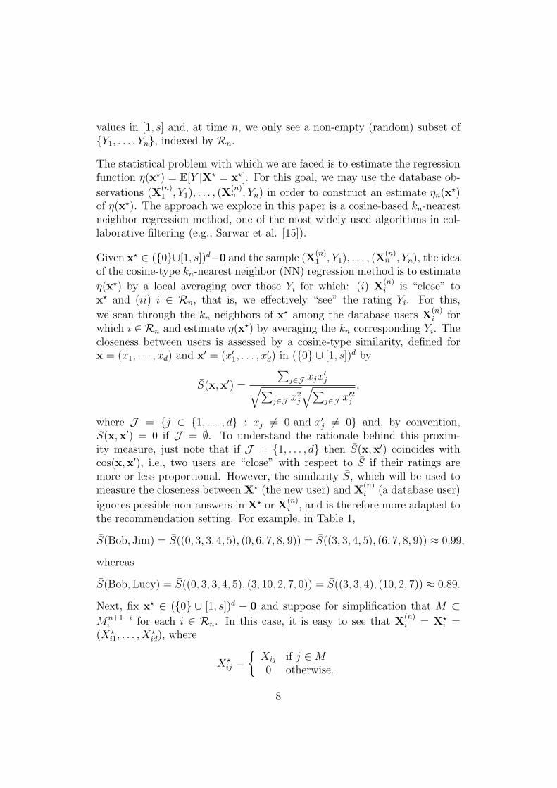
values in [1, s] and, at time n, we only see a non-empty (random) subset of{Y1, . . . , Yn}, indexed by Rn.
The statistical problem with which we are faced is to estimate the regressionfunction η(x?) = E[Y |X? = x?]. For this goal, we may use the database ob-
servations (X(n)1 , Y1), . . . , (X
(n)n , Yn) in order to construct an estimate ηn(x?)
of η(x?). The approach we explore in this paper is a cosine-based kn-nearestneighbor regression method, one of the most widely used algorithms in col-laborative filtering (e.g., Sarwar et al. [15]).
Given x? ∈ ({0}∪[1, s])d−0 and the sample (X(n)1 , Y1), . . . , (X
(n)n , Yn), the idea
of the cosine-type kn-nearest neighbor (NN) regression method is to estimate
η(x?) by a local averaging over those Yi for which: (i) X(n)i is “close” to
x? and (ii) i ∈ Rn, that is, we effectively “see” the rating Yi. For this,
we scan through the kn neighbors of x? among the database users X(n)i for
which i ∈ Rn and estimate η(x?) by averaging the kn corresponding Yi. Thecloseness between users is assessed by a cosine-type similarity, defined forx = (x1, . . . , xd) and x′ = (x′1, . . . , x
′d) in ({0} ∪ [1, s])d by
S(x,x′) =
∑j∈J xjx
′j√∑
j∈J x2j
√∑j∈J x
′2j
,
where J = {j ∈ {1, . . . , d} : xj 6= 0 and x′j 6= 0} and, by convention,S(x,x′) = 0 if J = ∅. To understand the rationale behind this proxim-ity measure, just note that if J = {1, . . . , d} then S(x,x′) coincides withcos(x,x′), i.e., two users are “close” with respect to S if their ratings aremore or less proportional. However, the similarity S, which will be used tomeasure the closeness between X? (the new user) and X
(n)i (a database user)
ignores possible non-answers in X? or X(n)i , and is therefore more adapted to
the recommendation setting. For example, in Table 1,
S(Bob, Jim) = S((0, 3, 3, 4, 5), (0, 6, 7, 8, 9)) = S((3, 3, 4, 5), (6, 7, 8, 9)) ≈ 0.99,
whereas
S(Bob,Lucy) = S((0, 3, 3, 4, 5), (3, 10, 2, 7, 0)) = S((3, 3, 4), (10, 2, 7)) ≈ 0.89.
Next, fix x? ∈ ({0} ∪ [1, s])d − 0 and suppose for simplification that M ⊂Mn+1−i
i for each i ∈ Rn. In this case, it is easy to see that X(n)i = X?
i =(X?
i1, . . . , X?id), where
X?ij =
{Xij if j ∈M0 otherwise.
8
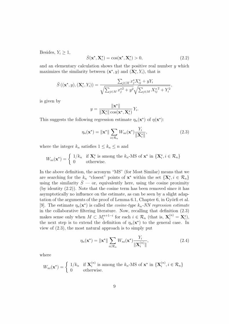
Besides, Yi ≥ 1,S(x?,X?
i ) = cos(x?,X?i ) > 0, (2.2)
and an elementary calculation shows that the positive real number y whichmaximizes the similarity between (x?, y) and (X?
i , Yi), that is
S ((x?, y), (X?i , Yi)) =
∑j∈M x?
jX?ij + yYi√∑
j∈M x?j2 + y2
√∑j∈M X?
ij2 + Y 2
i
,
is given by
y =‖x?‖
‖X?i ‖ cos(x?,X?
i )Yi.
This suggests the following regression estimate ηn(x?) of η(x?):
ηn(x?) = ‖x?‖∑i∈Rn
Wni(x?)
Yi
‖X?i ‖, (2.3)
where the integer kn satisfies 1 ≤ kn ≤ n and
Wni(x?) =
{1/kn if X?
i is among the kn-MS of x? in {X?i , i ∈ Rn}
0 otherwise.
In the above definition, the acronym “MS” (for Most Similar) means that weare searching for the kn “closest” points of x? within the set {X?
i , i ∈ Rn}using the similarity S — or, equivalently here, using the cosine proximity(by identity (2.2)). Note that the cosine term has been removed since it hasasymptotically no influence on the estimate, as can be seen by a slight adap-tation of the arguments of the proof of Lemma 6.1, Chapter 6, in Gyorfi et al.[9]. The estimate ηn(x?) is called the cosine-type kn-NN regression estimatein the collaborative filtering literature. Now, recalling that definition (2.3)
makes sense only when M ⊂ Mn+1−ii for each i ∈ Rn (that is, X
(n)i = X?
i ),the next step is to extend the definition of ηn(x?) to the general case. Inview of (2.3), the most natural approach is to simply put
ηn(x?) = ‖x?‖∑i∈Rn
Wni(x?)
Yi
‖X(n)i ‖
, (2.4)
where
Wni(x?) =
{1/kn if X
(n)i is among the kn-MS of x? in {X(n)
i , i ∈ Rn}0 otherwise.
9
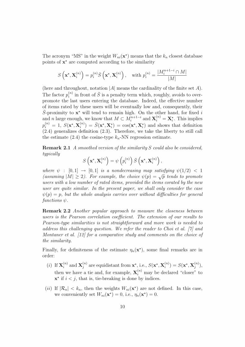
The acronym “MS” in the weight Wni(x?) means that the kn closest database
points of x? are computed according to the similarity
S(x?,X
(n)i
)= p
(n)i S
(x?,X
(n)i
), with p
(n)i =
|Mn+1−ii ∩M ||M |
(here and throughout, notation |A| means the cardinality of the finite set A).
The factor p(n)i in front of S is a penalty term which, roughly, avoids to over-
promote the last users entering the database. Indeed, the effective numberof items rated by these users will be eventually low and, consequently, theirS-proximity to x? will tend to remain high. On the other hand, for fixed iand n large enough, we know that M ⊂Mn+1−i
i and X(n)i = X?
i . This implies
p(n)i = 1, S(x?,X
(n)i ) = S(x?,X?
i ) = cos(x?,X?i ) and shows that definition
(2.4) generalizes definition (2.3). Therefore, we take the liberty to still callthe estimate (2.4) the cosine-type kn-NN regression estimate.
Remark 2.1 A smoothed version of the similarity S could also be considered,typically
S(x?,X
(n)i
)= ψ
(p
(n)i
)S(x?,X
(n)i
),
where ψ : [0, 1] → [0, 1] is a nondecreasing map satisfying ψ(1/2) < 1(assuming |M | ≥ 2). For example, the choice ψ(p) =
√p tends to promote
users with a low number of rated items, provided the items corated by the newuser are quite similar. In the present paper, we shall only consider the caseψ(p) = p, but the whole analysis carries over without difficulties for generalfunctions ψ.
Remark 2.2 Another popular approach to measure the closeness betweenusers is the Pearson correlation coefficient. The extension of our results toPearson-type similarities is not straightforward and more work is needed toaddress this challenging question. We refer the reader to Choi et al. [7] andMontaner et al. [12] for a comparative study and comments on the choice ofthe similarity.
Finally, for definiteness of the estimate ηn(x?), some final remarks are inorder:
(i) If X(n)i and X
(n)j are equidistant from x?, i.e., S(x?,X
(n)i ) = S(x?,X
(n)j ),
then we have a tie and, for example, X(n)i may be declared “closer” to
x? if i < j, that is, tie-breaking is done by indices.
(ii) If |Rn| < kn, then the weights Wni(x?) are not defined. In this case,
we conveniently set Wni(x?) = 0, i.e., ηn(x?) = 0.
10

(iii) If X(n)i = 0, then we take Wni(x
?) = 0 and we adopt the convention0×∞ = 0 for the computation of ηn(x?).
(iv) With the above conventions, the identity∑
i∈RnWni(x
?) ≤ 1 holds ineach case.
3 The regression function
Our objective in section 4 will be to establish consistency of the estimateηn(x?) defined in (2.4) towards the regression function η(x?). To reach thisgoal, we first need to analyze the properties of η(x?). Surprisingly, the specialform of ηn(x?) constrains the shape of η(x?). This is stated in Theorem 3.1below.
Theorem 3.1 Suppose that ηn(X?)→ η(X?) in probability as n→∞. Then
η(X?) = ‖X?‖E[
Y
‖X?‖
∣∣∣ X?
‖X?‖
]a.s.
Proof of Theorem 3.1. Recall that
ηn(X?) = ‖X?‖∑i∈Rn
Wni(X?)
Yi
‖X(n)i ‖
,
and let
ϕn(X?) =∑i∈Rn
Wni(X?)
Yi
‖X(n)i ‖
.
Since (ηn(X?))n is a Cauchy sequence in probability and ‖X?‖ ≥ 1, (ϕn(X?))n
is also a Cauchy sequence. Thus, there exists a measurable function ϕ on Rd
such that ϕn(X?)→ ϕ(X?) in probability. Using the fact that 0 ≤ ϕn(X?) ≤s for all n ≥ 1, we conclude that 0 ≤ ϕ(X?) ≤ s a.s. as well.
Let us extract a sequence (nk)k satisfying ϕnk(X?)→ ϕ(X?) a.s. Observing
that, for x? 6= 0,
ϕnk(x?) = ϕnk
(x?
‖x?‖
),
we may write ϕ(X?) = ϕ(X?/‖X?‖) a.s. Consequently, the limit in proba-bility of (ηn(X?))n is
‖X?‖ϕ(
X?
‖X?‖
).
11
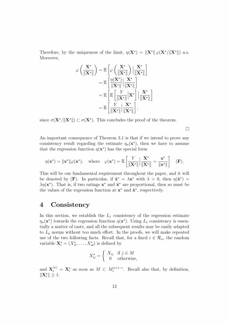
Therefore, by the uniqueness of the limit, η(X?) = ‖X?‖ϕ(X?/‖X?‖) a.s.Moreover,
ϕ
(X?
‖X?‖
)= E
[ϕ
(X?
‖X?‖
) ∣∣∣ X?
‖X?‖
]= E
[η(X?)
‖X?‖
∣∣∣ X?
‖X?‖
]= E
[E[
Y
‖X?‖
∣∣∣X?
] ∣∣∣ X?
‖X?‖
]= E
[Y
‖X?‖
∣∣∣ X?
‖X?‖
],
since σ(X?/‖X?‖) ⊂ σ(X?). This concludes the proof of the theorem.
�
An important consequence of Theorem 3.1 is that if we intend to prove anyconsistency result regarding the estimate ηn(x?), then we have to assumethat the regression function η(x?) has the special form
η(x?) = ‖x?‖ϕ(x?), where ϕ(x?) = E[
Y
‖X?‖
∣∣∣ X?
‖X?‖=
x?
‖x?‖
](F).
This will be our fundamental requirement throughout the paper, and it willbe denoted by (F). In particular, if x? = λx? with λ > 0, then η(x?) =λη(x?). That is, if two ratings x? and x? are proportional, then so must bethe values of the regression function at x? and x?, respectively.
4 Consistency
In this section, we establish the L1 consistency of the regression estimateηn(x?) towards the regression function η(x?). Using L1 consistency is essen-tially a matter of taste, and all the subsequent results may be easily adaptedto Lp norms without too much effort. In the proofs, we will make repeateduse of the two following facts. Recall that, for a fixed i ∈ Rn, the randomvariable X?
i = (X?i1, . . . , X
?id) is defined by
X?ij =
{Xij if j ∈M0 otherwise,
and X(n)i = X?
i as soon as M ⊂ Mn+1−ii . Recall also that, by definition,
‖X?i ‖ ≥ 1.
12
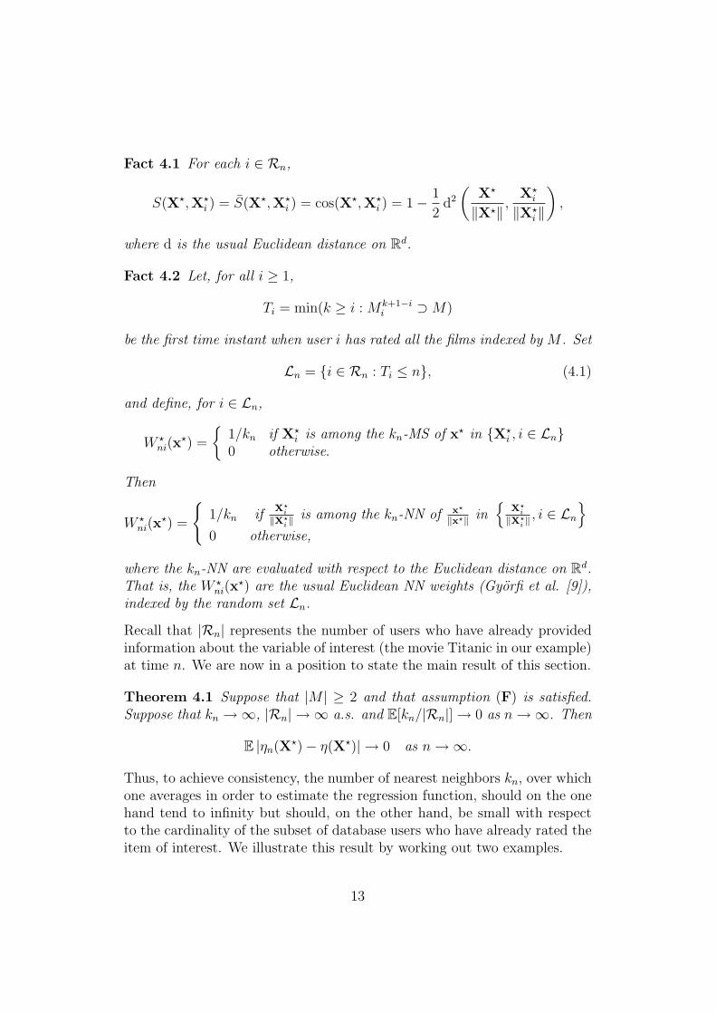
Fact 4.1 For each i ∈ Rn,
S(X?,X?i ) = S(X?,X?
i ) = cos(X?,X?i ) = 1− 1
2d2
(X?
‖X?‖,
X?i
‖X?i ‖
),
where d is the usual Euclidean distance on Rd.
Fact 4.2 Let, for all i ≥ 1,
Ti = min(k ≥ i : Mk+1−ii ⊃M)
be the first time instant when user i has rated all the films indexed by M . Set
Ln = {i ∈ Rn : Ti ≤ n}, (4.1)
and define, for i ∈ Ln,
W ?ni(x
?) =
{1/kn if X?
i is among the kn-MS of x? in {X?i , i ∈ Ln}
0 otherwise.
Then
W ?ni(x
?) =
{1/kn if
X?i
‖X?i ‖
is among the kn-NN of x?
‖x?‖ in{
X?i
‖X?i ‖, i ∈ Ln
}0 otherwise,
where the kn-NN are evaluated with respect to the Euclidean distance on Rd.That is, the W ?
ni(x?) are the usual Euclidean NN weights (Gyorfi et al. [9]),
indexed by the random set Ln.
Recall that |Rn| represents the number of users who have already providedinformation about the variable of interest (the movie Titanic in our example)at time n. We are now in a position to state the main result of this section.
Theorem 4.1 Suppose that |M | ≥ 2 and that assumption (F) is satisfied.Suppose that kn →∞, |Rn| → ∞ a.s. and E[kn/|Rn|]→ 0 as n→∞. Then
E |ηn(X?)− η(X?)| → 0 as n→∞.
Thus, to achieve consistency, the number of nearest neighbors kn, over whichone averages in order to estimate the regression function, should on the onehand tend to infinity but should, on the other hand, be small with respectto the cardinality of the subset of database users who have already rated theitem of interest. We illustrate this result by working out two examples.
13
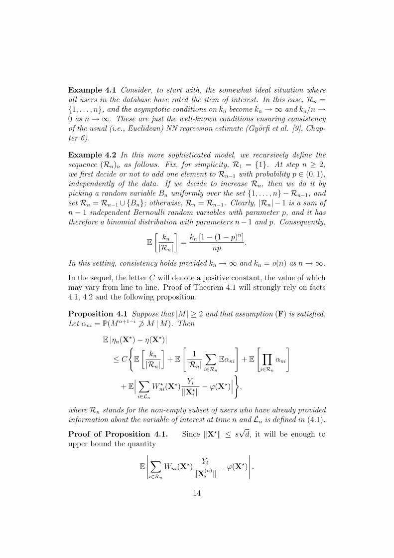
Example 4.1 Consider, to start with, the somewhat ideal situation whereall users in the database have rated the item of interest. In this case, Rn ={1, . . . , n}, and the asymptotic conditions on kn become kn →∞ and kn/n→0 as n→∞. These are just the well-known conditions ensuring consistencyof the usual (i.e., Euclidean) NN regression estimate (Gyorfi et al. [9], Chap-ter 6).
Example 4.2 In this more sophisticated model, we recursively define thesequence (Rn)n as follows. Fix, for simplicity, R1 = {1}. At step n ≥ 2,we first decide or not to add one element to Rn−1 with probability p ∈ (0, 1),independently of the data. If we decide to increase Rn, then we do it bypicking a random variable Bn uniformly over the set {1, . . . , n} −Rn−1, andset Rn = Rn−1 ∪{Bn}; otherwise, Rn = Rn−1. Clearly, |Rn| − 1 is a sum ofn − 1 independent Bernoulli random variables with parameter p, and it hastherefore a binomial distribution with parameters n− 1 and p. Consequently,
E[kn
|Rn|
]=kn [1− (1− p)n]
np.
In this setting, consistency holds provided kn →∞ and kn = o(n) as n→∞.
In the sequel, the letter C will denote a positive constant, the value of whichmay vary from line to line. Proof of Theorem 4.1 will strongly rely on facts4.1, 4.2 and the following proposition.
Proposition 4.1 Suppose that |M | ≥ 2 and that assumption (F) is satisfied.Let αni = P(Mn+1−i 6⊃M |M). Then
E |ηn(X?)− η(X?)|
≤ C
{E[kn
|Rn|
]+ E
[1
|Rn|∑i∈Rn
Eαni
]+ E
[∏i∈Rn
αni
]
+ E∣∣∣∑
i∈Ln
W ?ni(X
?)Yi
‖X?i ‖− ϕ(X?)
∣∣∣},where Rn stands for the non-empty subset of users who have already providedinformation about the variable of interest at time n and Ln is defined in (4.1).
Proof of Proposition 4.1. Since ‖X?‖ ≤ s√d, it will be enough to
upper bound the quantity
E
∣∣∣∣∣∑i∈Rn
Wni(X?)
Yi
‖X(n)i ‖− ϕ(X?)
∣∣∣∣∣ .14
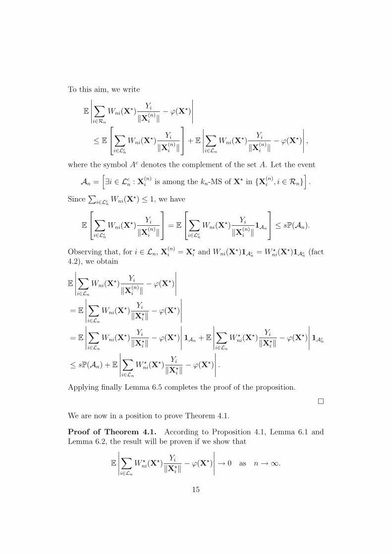
To this aim, we write
E
∣∣∣∣∣∑i∈Rn
Wni(X?)
Yi
‖X(n)i ‖− ϕ(X?)
∣∣∣∣∣≤ E
∑i∈Lc
n
Wni(X?)
Yi
‖X(n)i ‖
+ E
∣∣∣∣∣∑i∈Ln
Wni(X?)
Yi
‖X(n)i ‖− ϕ(X?)
∣∣∣∣∣ ,where the symbol Ac denotes the complement of the set A. Let the event
An =[∃i ∈ Lc
n : X(n)i is among the kn-MS of X? in {X(n)
i , i ∈ Rn}].
Since∑
i∈LcnWni(X
?) ≤ 1, we have
E
∑i∈Lc
n
Wni(X?)
Yi
‖X(n)i ‖
= E
∑i∈Lc
n
Wni(X?)
Yi
‖X(n)i ‖
1An
≤ sP(An).
Observing that, for i ∈ Ln, X(n)i = X?
i and Wni(X?)1Ac
n= W ?
ni(X?)1Ac
n(fact
4.2), we obtain
E
∣∣∣∣∣∑i∈Ln
Wni(X?)
Yi
‖X(n)i ‖− ϕ(X?)
∣∣∣∣∣= E
∣∣∣∣∣∑i∈Ln
Wni(X?)
Yi
‖X?i ‖− ϕ(X?)
∣∣∣∣∣= E
∣∣∣∣∣∑i∈Ln
Wni(X?)
Yi
‖X?i ‖− ϕ(X?)
∣∣∣∣∣1An + E
∣∣∣∣∣∑i∈Ln
W ?ni(X
?)Yi
‖X?i ‖− ϕ(X?)
∣∣∣∣∣1Acn
≤ sP(An) + E
∣∣∣∣∣∑i∈Ln
W ?ni(X
?)Yi
‖X?i ‖− ϕ(X?)
∣∣∣∣∣ .Applying finally Lemma 6.5 completes the proof of the proposition.
�
We are now in a position to prove Theorem 4.1.
Proof of Theorem 4.1. According to Proposition 4.1, Lemma 6.1 andLemma 6.2, the result will be proven if we show that
E
∣∣∣∣∣∑i∈Ln
W ?ni(X
?)Yi
‖X?i ‖− ϕ(X?)
∣∣∣∣∣→ 0 as n→∞.
15
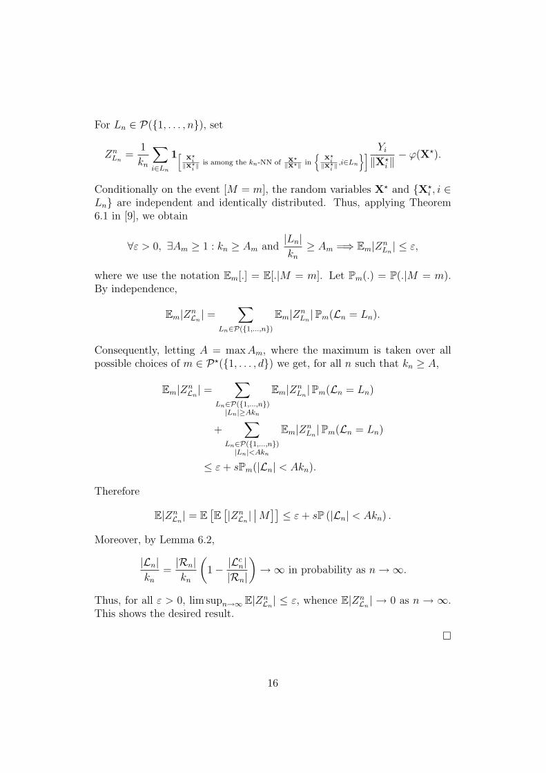
For Ln ∈ P({1, . . . , n}), set
ZnLn
=1
kn
∑i∈Ln
1»X?
i‖X?
i‖ is among the kn-NN of X?
‖X?‖ in
X?
i‖X?
i‖ ,i∈Ln
ff– Yi
‖X?i ‖− ϕ(X?).
Conditionally on the event [M = m], the random variables X? and {X?i , i ∈
Ln} are independent and identically distributed. Thus, applying Theorem6.1 in [9], we obtain
∀ε > 0, ∃Am ≥ 1 : kn ≥ Am and|Ln|kn
≥ Am =⇒ Em|ZnLn| ≤ ε,
where we use the notation Em[.] = E[.|M = m]. Let Pm(.) = P(.|M = m).By independence,
Em|ZnLn| =
∑Ln∈P({1,...,n})
Em|ZnLn|Pm(Ln = Ln).
Consequently, letting A = maxAm, where the maximum is taken over allpossible choices of m ∈ P?({1, . . . , d}) we get, for all n such that kn ≥ A,
Em|ZnLn| =
∑Ln∈P({1,...,n})|Ln|≥Akn
Em|ZnLn|Pm(Ln = Ln)
+∑
Ln∈P({1,...,n})|Ln|<Akn
Em|ZnLn|Pm(Ln = Ln)
≤ ε+ sPm(|Ln| < Akn).
Therefore
E|ZnLn| = E
[E[|ZnLn|∣∣M]] ≤ ε+ sP (|Ln| < Akn) .
Moreover, by Lemma 6.2,
|Ln|kn
=|Rn|kn
(1− |L
cn|
|Rn|
)→∞ in probability as n→∞.
Thus, for all ε > 0, lim supn→∞ E|ZnLn| ≤ ε, whence E|Zn
Ln| → 0 as n → ∞.
This shows the desired result.
�
16
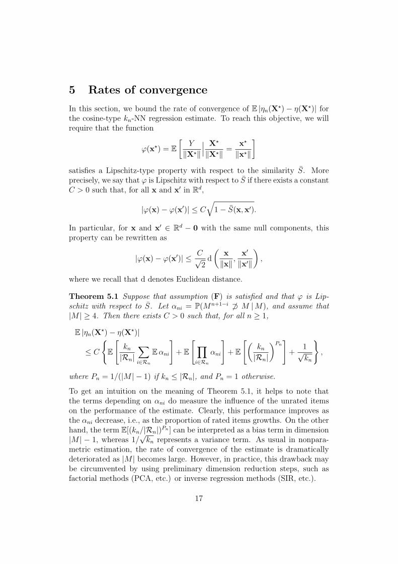
5 Rates of convergence
In this section, we bound the rate of convergence of E |ηn(X?)− η(X?)| forthe cosine-type kn-NN regression estimate. To reach this objective, we willrequire that the function
ϕ(x?) = E[
Y
‖X?‖
∣∣∣ X?
‖X?‖=
x?
‖x?‖
]satisfies a Lipschitz-type property with respect to the similarity S. Moreprecisely, we say that ϕ is Lipschitz with respect to S if there exists a constantC > 0 such that, for all x and x′ in Rd,
|ϕ(x)− ϕ(x′)| ≤ C√
1− S(x,x′).
In particular, for x and x′ ∈ Rd − 0 with the same null components, thisproperty can be rewritten as
|ϕ(x)− ϕ(x′)| ≤ C√2
d
(x
‖x‖,
x′
‖x′‖
),
where we recall that d denotes Euclidean distance.
Theorem 5.1 Suppose that assumption (F) is satisfied and that ϕ is Lip-schitz with respect to S. Let αni = P(Mn+1−i 6⊃ M |M), and assume that|M | ≥ 4. Then there exists C > 0 such that, for all n ≥ 1,
E |ηn(X?)− η(X?)|
≤ C
{E
[kn
|Rn|∑i∈Rn
Eαni
]+ E
[∏i∈Rn
αni
]+ E
[(kn
|Rn|
)Pn]
+1√kn
},
where Pn = 1/(|M | − 1) if kn ≤ |Rn|, and Pn = 1 otherwise.
To get an intuition on the meaning of Theorem 5.1, it helps to note thatthe terms depending on αni do measure the influence of the unrated itemson the performance of the estimate. Clearly, this performance improves asthe αni decrease, i.e., as the proportion of rated items growths. On the otherhand, the term E[(kn/|Rn|)Pn ] can be interpreted as a bias term in dimension|M | − 1, whereas 1/
√kn represents a variance term. As usual in nonpara-
metric estimation, the rate of convergence of the estimate is dramaticallydeteriorated as |M | becomes large. However, in practice, this drawback maybe circumvented by using preliminary dimension reduction steps, such asfactorial methods (PCA, etc.) or inverse regression methods (SIR, etc.).
17
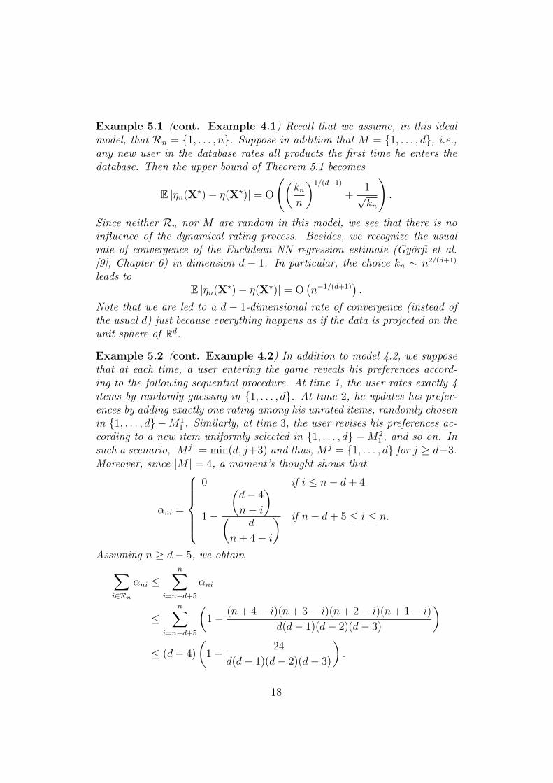
Example 5.1 (cont. Example 4.1) Recall that we assume, in this idealmodel, that Rn = {1, . . . , n}. Suppose in addition that M = {1, . . . , d}, i.e.,any new user in the database rates all products the first time he enters thedatabase. Then the upper bound of Theorem 5.1 becomes
E |ηn(X?)− η(X?)| = O
((kn
n
)1/(d−1)
+1√kn
).
Since neither Rn nor M are random in this model, we see that there is noinfluence of the dynamical rating process. Besides, we recognize the usualrate of convergence of the Euclidean NN regression estimate (Gyorfi et al.[9], Chapter 6) in dimension d − 1. In particular, the choice kn ∼ n2/(d+1)
leads toE |ηn(X?)− η(X?)| = O
(n−1/(d+1)
).
Note that we are led to a d − 1-dimensional rate of convergence (instead ofthe usual d) just because everything happens as if the data is projected on theunit sphere of Rd.
Example 5.2 (cont. Example 4.2) In addition to model 4.2, we supposethat at each time, a user entering the game reveals his preferences accord-ing to the following sequential procedure. At time 1, the user rates exactly 4items by randomly guessing in {1, . . . , d}. At time 2, he updates his prefer-ences by adding exactly one rating among his unrated items, randomly chosenin {1, . . . , d} −M1
1 . Similarly, at time 3, the user revises his preferences ac-cording to a new item uniformly selected in {1, . . . , d} −M2
1 , and so on. Insuch a scenario, |M j| = min(d, j+3) and thus, M j = {1, . . . , d} for j ≥ d−3.Moreover, since |M | = 4, a moment’s thought shows that
αni =
0 if i ≤ n− d+ 4
1−
(d− 4
n− i
)(
d
n+ 4− i
) if n− d+ 5 ≤ i ≤ n.
Assuming n ≥ d− 5, we obtain∑i∈Rn
αni ≤n∑
i=n−d+5
αni
≤n∑
i=n−d+5
(1− (n+ 4− i)(n+ 3− i)(n+ 2− i)(n+ 1− i)
d(d− 1)(d− 2)(d− 3)
)≤ (d− 4)
(1− 24
d(d− 1)(d− 2)(d− 3)
).
18
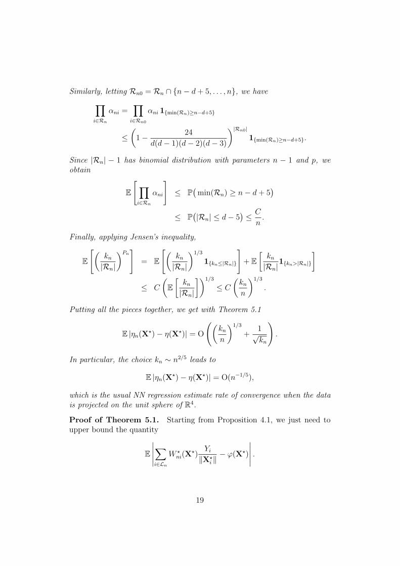
Similarly, letting Rn0 = Rn ∩ {n− d+ 5, . . . , n}, we have∏i∈Rn
αni =∏
i∈Rn0
αni 1{min(Rn)≥n−d+5}
≤(
1− 24
d(d− 1)(d− 2)(d− 3)
)|Rn0|
1{min(Rn)≥n−d+5}.
Since |Rn| − 1 has binomial distribution with parameters n − 1 and p, weobtain
E
[∏i∈Rn
αni
]≤ P
(min(Rn) ≥ n− d+ 5
)≤ P
(|Rn| ≤ d− 5
)≤ C
n.
Finally, applying Jensen’s inequality,
E
[(kn
|Rn|
)Pn]
= E
[(kn
|Rn|
)1/3
1{kn≤|Rn|}
]+ E
[kn
|Rn|1{kn>|Rn|}
]
≤ C
(E[kn
|Rn|
])1/3
≤ C
(kn
n
)1/3
.
Putting all the pieces together, we get with Theorem 5.1
E |ηn(X?)− η(X?)| = O
((kn
n
)1/3
+1√kn
).
In particular, the choice kn ∼ n2/5 leads to
E |ηn(X?)− η(X?)| = O(n−1/5),
which is the usual NN regression estimate rate of convergence when the datais projected on the unit sphere of R4.
Proof of Theorem 5.1. Starting from Proposition 4.1, we just need toupper bound the quantity
E
∣∣∣∣∣∑i∈Ln
W ?ni(X
?)Yi
‖X?i ‖− ϕ(X?)
∣∣∣∣∣ .
19
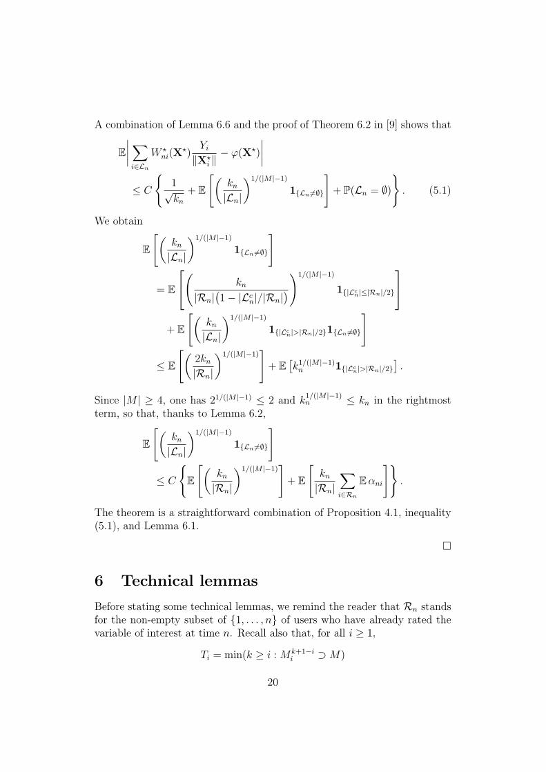
A combination of Lemma 6.6 and the proof of Theorem 6.2 in [9] shows that
E∣∣∣∣∑
i∈Ln
W ?ni(X
?)Yi
‖X?i ‖− ϕ(X?)
∣∣∣∣≤ C
{1√kn
+ E
[(kn
|Ln|
)1/(|M |−1)
1{Ln 6=∅}
]+ P(Ln = ∅)
}. (5.1)
We obtain
E
[(kn
|Ln|
)1/(|M |−1)
1{Ln 6=∅}
]
= E
( kn
|Rn|(1− |Lc
n|/|Rn|))1/(|M |−1)
1{|Lcn|≤|Rn|/2}
+ E
[(kn
|Ln|
)1/(|M |−1)
1{|Lcn|>|Rn|/2}1{Ln 6=∅}
]
≤ E
[(2kn
|Rn|
)1/(|M |−1)]
+ E[k1/(|M |−1)
n 1{|Lcn|>|Rn|/2}
].
Since |M | ≥ 4, one has 21/(|M |−1) ≤ 2 and k1/(|M |−1)n ≤ kn in the rightmost
term, so that, thanks to Lemma 6.2,
E
[(kn
|Ln|
)1/(|M |−1)
1{Ln 6=∅}
]
≤ C
{E
[(kn
|Rn|
)1/(|M |−1)]
+ E
[kn
|Rn|∑i∈Rn
Eαni
]}.
The theorem is a straightforward combination of Proposition 4.1, inequality(5.1), and Lemma 6.1.
�
6 Technical lemmas
Before stating some technical lemmas, we remind the reader that Rn standsfor the non-empty subset of {1, . . . , n} of users who have already rated thevariable of interest at time n. Recall also that, for all i ≥ 1,
Ti = min(k ≥ i : Mk+1−ii ⊃M)
20

andLn = {i ∈ Rn : Ti ≤ n}.
Lemma 6.1 We have
P(Ln = ∅) = E
[∏i∈Rn
αni
]→ 0 as n→∞.
Proof of Lemma 6.1. Conditionally on M and Rn, the random variables{Ti, i ∈ Rn} are independent. Moreover, the sequence (Mn)n≥1 is nonde-creasing. Thus, the identity [Ti > n] = [Mn+1−i
i 6⊃ M ] holds for all i ∈ Rn.Hence,
P(Ln = ∅) = P (∀i ∈ Rn : Ti > n)
= E[P(∀i ∈ Rn : Ti > n
∣∣∣Rn,M)]
= E
[∏i∈Rn
P(Ti > n
∣∣∣Rn,M)]
= E
[∏i∈Rn
P(Mn+1−i
i 6⊃M∣∣∣M)]
(by independence of (Mn+1−ii ,M) and Rn)
= E
[∏i∈Rn
αni
].
The last statement of the lemma is clear since, for all i, αni → 0 a.s. asn→∞.
�
Lemma 6.2 We have
E[|Lc
n||Rn|
]= E
[1
|Rn|∑i∈Rn
Eαni
]and
E[
1
|Ln|1{Ln 6=∅}
]≤ 2E
[1
|Rn|
]+ 2E
[1
|Rn|∑i∈Rn
Eαni
].
Moreover, if limn→∞ |Rn| =∞ a.s., then
limn→∞
E[|Lc
n||Rn|
]= 0.
21

Proof of Lemma 6.2. First, using the fact that the sequence (Mn)n≥1 isnondecreasing, we see that for all i ∈ Rn, [Ti > n] = [Mn+1−i
i 6⊃ M ]. Next,recalling that Rn is independent of Ti for fixed i, we obtain
E[|Lc
n||Rn|
∣∣∣Rn
]=
1
|Rn|E
[∑i∈Rn
1{Ti>n}
∣∣∣Rn
]=
1
|Rn|∑i∈Rn
P(Mn+1−ii 6⊃M),
and this proves the first statement of the lemma. Now define Jn = {n+ 1−i, i ∈ Rn} and observe that
E[|Lc
n||Rn|
]= E
[1
|Jn|∑j∈Jn
P(M j 6⊃M)
],
where we used |Jn| = |Rn|. Since, by assumption, |Jn| = |Rn| → ∞ a.s. asn→∞ and P(M j 6⊃M)→ 0 as j →∞, we obtain
limn→∞
1
|Jn|∑j∈Jn
P(M j 6⊃M) = 0 a.s.
The conclusion follows by applying Lebesgue’s dominated convergence The-orem. The second statement of the lemma is obtained from the followingchain of inequalities:
E[
1
|Ln|1{Ln 6=∅}
]= E
[1
|Rn|(1− |Lc
n|/|Rn|)1{Ln 6=∅}
]
= E
[1
|Rn|(1− |Lc
n|/|Rn|)1{|Lc
n|≤|Rn|/2}
]
+E[
1
|Ln|1{|Lc
n|>|Rn|/2}1{Ln 6=∅}
]≤ 2E
[1
|Rn|
]+ P
(|Lc
n| >|Rn|
2
)≤ 2E
[1
|Rn|
]+ 2E
[|Lc
n||Rn|
].
Applying the first part of the lemma completes the proof.
�
22
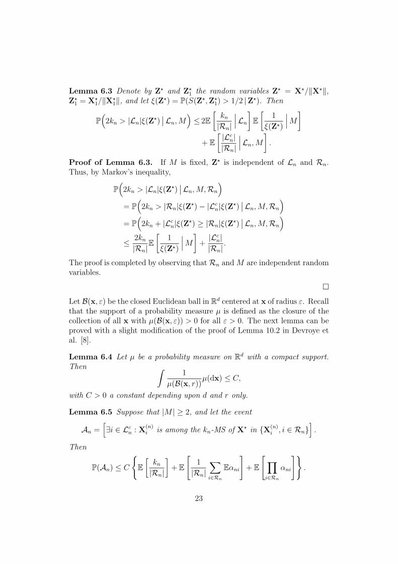
Lemma 6.3 Denote by Z? and Z?1 the random variables Z? = X?/‖X?‖,
Z?1 = X?
1/‖X?1‖, and let ξ(Z?) = P(S(Z?,Z?
1) > 1/2 |Z?). Then
P(
2kn > |Ln|ξ(Z?)∣∣Ln,M
)≤ 2E
[kn
|Rn|
∣∣∣Ln
]E[
1
ξ(Z?)
∣∣∣M]+ E
[|Lc
n||Rn|
∣∣∣Ln,M
].
Proof of Lemma 6.3. If M is fixed, Z? is independent of Ln and Rn.Thus, by Markov’s inequality,
P(
2kn > |Ln|ξ(Z?)∣∣Ln,M,Rn
)= P
(2kn > |Rn|ξ(Z?)− |Lc
n|ξ(Z?)∣∣Ln,M,Rn
)= P
(2kn + |Lc
n|ξ(Z?) ≥ |Rn|ξ(Z?)∣∣Ln,M,Rn
)≤ 2kn
|Rn|E[
1
ξ(Z?)
∣∣∣M]+|Lc
n||Rn|
.
The proof is completed by observing thatRn and M are independent randomvariables.
�
Let B(x, ε) be the closed Euclidean ball in Rd centered at x of radius ε. Recallthat the support of a probability measure µ is defined as the closure of thecollection of all x with µ(B(x, ε)) > 0 for all ε > 0. The next lemma can beproved with a slight modification of the proof of Lemma 10.2 in Devroye etal. [8].
Lemma 6.4 Let µ be a probability measure on Rd with a compact support.Then ∫
1
µ(B(x, r))µ(dx) ≤ C,
with C > 0 a constant depending upon d and r only.
Lemma 6.5 Suppose that |M | ≥ 2, and let the event
An =[∃i ∈ Lc
n : X(n)i is among the kn-MS of X? in {X(n)
i , i ∈ Rn}].
Then
P(An) ≤ C
{E[kn
|Rn|
]+ E
[1
|Rn|∑i∈Rn
Eαni
]+ E
[∏i∈Rn
αni
]}.
23
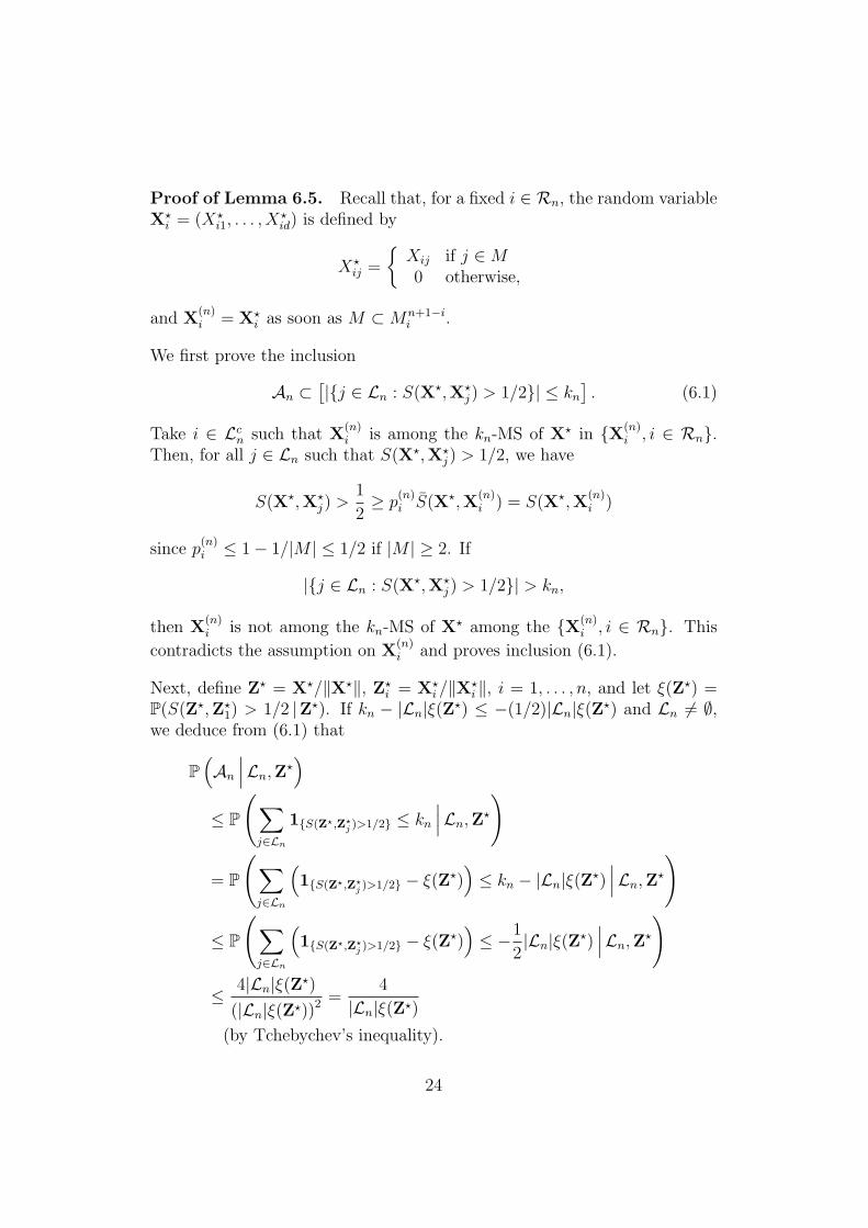
Proof of Lemma 6.5. Recall that, for a fixed i ∈ Rn, the random variableX?
i = (X?i1, . . . , X
?id) is defined by
X?ij =
{Xij if j ∈M0 otherwise,
and X(n)i = X?
i as soon as M ⊂Mn+1−ii .
We first prove the inclusion
An ⊂[|{j ∈ Ln : S(X?,X?
j) > 1/2}| ≤ kn
]. (6.1)
Take i ∈ Lcn such that X
(n)i is among the kn-MS of X? in {X(n)
i , i ∈ Rn}.Then, for all j ∈ Ln such that S(X?,X?
j) > 1/2, we have
S(X?,X?j) >
1
2≥ p
(n)i S(X?,X
(n)i ) = S(X?,X
(n)i )
since p(n)i ≤ 1− 1/|M | ≤ 1/2 if |M | ≥ 2. If
|{j ∈ Ln : S(X?,X?j) > 1/2}| > kn,
then X(n)i is not among the kn-MS of X? among the {X(n)
i , i ∈ Rn}. This
contradicts the assumption on X(n)i and proves inclusion (6.1).
Next, define Z? = X?/‖X?‖, Z?i = X?
i /‖X?i ‖, i = 1, . . . , n, and let ξ(Z?) =
P(S(Z?,Z?1) > 1/2 |Z?). If kn − |Ln|ξ(Z?) ≤ −(1/2)|Ln|ξ(Z?) and Ln 6= ∅,
we deduce from (6.1) that
P(An
∣∣∣Ln,Z?)
≤ P
(∑j∈Ln
1{S(Z?,Z?j )>1/2} ≤ kn
∣∣∣Ln,Z?
)
= P
(∑j∈Ln
(1{S(Z?,Z?
j )>1/2} − ξ(Z?))≤ kn − |Ln|ξ(Z?)
∣∣∣Ln,Z?
)
≤ P
(∑j∈Ln
(1{S(Z?,Z?
j )>1/2} − ξ(Z?))≤ −1
2|Ln|ξ(Z?)
∣∣∣Ln,Z?
)
≤ 4|Ln|ξ(Z?)
(|Ln|ξ(Z?))2 =4
|Ln|ξ(Z?)
(by Tchebychev’s inequality).
24

In the last inequality, we use the fact that, since σ(M) ⊂ σ(Z?), the randomvariables {Z?
i , i ∈ Ln} are independent conditionally on Z? and Ln. Usingagain the inclusion σ(M) ⊂ σ(Z?), we obtain, on the event [Ln 6= 0],
P(An
∣∣∣Ln,M)
= E[P(An
∣∣∣Ln,Z?) ∣∣∣Ln,M
]≤ 4
|Ln|E[
1
ξ(Z?)
∣∣∣Ln,M
]+ P
(kn − |Ln|ξ(Z?) > −1
2|Ln|ξ(Z?)
∣∣∣Ln,M
)=
4
|Ln|E[
1
ξ(Z?)
∣∣∣M]+ P(|Ln|ξ(Z?) < 2kn
∣∣∣Ln,M).
Applying Lemma 6.3, on the event [Ln 6= ∅],
P(An
∣∣∣Ln,M)
≤ 4
|Ln|E[
1
ξ(Z?)
∣∣∣M]+ 2E[kn
|Rn|
∣∣∣Ln
]E[
1
ξ(Z?)
∣∣∣M]+ E[|Lc
n||Rn|
∣∣∣Ln,M
].
Moreover, by fact 4.1,
ξ(Z?) = P(S(Z?,Z?
1) >1
2
∣∣∣Z?
)≥ P
(d2(Z?,Z?
1) ≤1
2
∣∣∣Z?
).
Thus, denoting by νM the distribution of Z? conditionally to M , we deducefrom Lemma 6.4 that
E[
1
ξ(Z?)
∣∣∣M] ≤ ∫ 1
νM(B(z, 1/√
2))νM(dz) ≤ C,
where the constant C does not depend on M . Putting all the pieces together,we obtain
P(An) ≤ C
{E[
1
|Ln|1{Ln 6=∅}
]+ E
[kn
|Rn|
]+ E
[|Lc
n||Rn|
]}+ P(Ln = ∅).
We conclude the proof with Lemma 6.1 and Lemma 6.2.
�
In the sequel, we let X?(1), . . . ,X
?(|Ln|) be the sequence {X?
i , i ∈ Ln} reordered
according to decreasing similarities S(X?,X?i ), i ∈ Ln, that is,
S(X?,X?
(1)
)≥ . . . ≥ S
(X?,X?
(|Ln|)).
Lemma 6.6 below states the rate of convergence to 1 of S(X?,X?(1)).
25
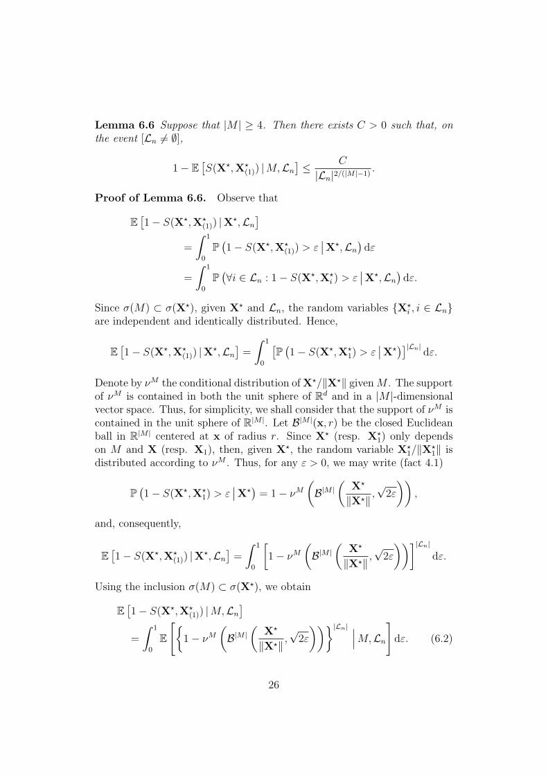
Lemma 6.6 Suppose that |M | ≥ 4. Then there exists C > 0 such that, onthe event [Ln 6= ∅],
1− E[S(X?,X?
(1)) |M,Ln
]≤ C
|Ln|2/(|M |−1).
Proof of Lemma 6.6. Observe that
E[1− S(X?,X?
(1)) |X?,Ln
]=
∫ 1
0
P(1− S(X?,X?
(1)) > ε∣∣X?,Ln
)dε
=
∫ 1
0
P(∀i ∈ Ln : 1− S(X?,X?
i ) > ε∣∣X?,Ln
)dε.
Since σ(M) ⊂ σ(X?), given X? and Ln, the random variables {X?i , i ∈ Ln}
are independent and identically distributed. Hence,
E[1− S(X?,X?
(1)) |X?,Ln
]=
∫ 1
0
[P(1− S(X?,X?
1) > ε∣∣X?
)]|Ln|dε.
Denote by νM the conditional distribution of X?/‖X?‖ given M . The supportof νM is contained in both the unit sphere of Rd and in a |M |-dimensionalvector space. Thus, for simplicity, we shall consider that the support of νM iscontained in the unit sphere of R|M |. Let B|M |(x, r) be the closed Euclideanball in R|M | centered at x of radius r. Since X? (resp. X?
1) only dependson M and X (resp. X1), then, given X?, the random variable X?
1/‖X?1‖ is
distributed according to νM . Thus, for any ε > 0, we may write (fact 4.1)
P(1− S(X?,X?
1) > ε∣∣X?
)= 1− νM
(B|M |
(X?
‖X?‖,√
2ε
)),
and, consequently,
E[1− S(X?,X?
(1)) |X?,Ln
]=
∫ 1
0
[1− νM
(B|M |
(X?
‖X?‖,√
2ε
))]|Ln|
dε.
Using the inclusion σ(M) ⊂ σ(X?), we obtain
E[1− S(X?,X?
(1)) |M,Ln
]=
∫ 1
0
E
[{1− νM
(B|M |
(X?
‖X?‖,√
2ε
))}|Ln| ∣∣∣M,Ln
]dε. (6.2)
26
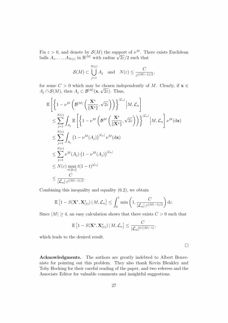
Fix ε > 0, and denote by S(M) the support of νM . There exists Euclideanballs A1, . . . , AN(ε) in R|M | with radius
√2ε/2 such that
S(M) ⊂N(ε)⋃j=1
Aj and N(ε) ≤ C
ε(|M |−1)/2,
for some C > 0 which may be chosen independently of M . Clearly, if x ∈Aj ∩ S(M), then Aj ⊂ B|M |(x,
√2ε). Thus,
E
[{1− νM
(B|M |
(X?
‖X?‖,√
2ε
))}|Ln| ∣∣∣M,Ln
]
≤N(ε)∑j=1
∫Aj
E
[{1− νM
(BM
(X?
‖X?‖,√
2ε
))}|Ln| ∣∣∣M,Ln
]νM(dx)
≤N(ε)∑j=1
∫Aj
(1− νM(Aj)
)|Ln|νM(dx)
≤N(ε)∑j=1
νM(Aj)(1− νM(Aj)
)|Ln|
≤ N(ε) maxt∈[0,1]
t(1− t)|Ln|
≤ C
|Ln| ε(|M |−1)/2.
Combining this inequality and equality (6.2), we obtain
E[1− S(X?,X?
(1)) |M,Ln
]≤∫ 1
0
min
(1,
C
|Ln| ε(|M |−1)/2
)dε.
Since |M | ≥ 4, an easy calculation shows that there exists C > 0 such that
E[1− S(X?,X?
(1)) |M,Ln
]≤ C
|Ln|2/(|M |−1),
which leads to the desired result.
�
Acknowledgments. The authors are greatly indebted to Albert Benve-niste for pointing out this problem. They also thank Kevin Bleakley andToby Hocking for their careful reading of the paper, and two referees and theAssociate Editor for valuable comments and insightful suggestions.
27
References
[1] J. Abernethy, F.R. Bach, T. Evgeniou, and J.-P. Vert. A new approachto collaborative filtering: Operator estimation with spectral regulariza-tion. J. Mach. Learn. Res., 10:803–826, 2009.
[2] G. Adomavicius, R. Sankaranarayanan, S. Sen, and A. Tuzhilin. Incor-porating contextual information in recommender systems using a mul-tidimensional approach. ACM Trans. Info. Syst., 2005.
[3] G. Adomavicius and A. Tuzhilin. Toward the next generation of rec-ommender systems: A survey of the state-of-the-art and possible exten-sions. IEEE Trans. Knowl. Data Eng., 17:734–749, 2005.
[4] J.S. Breese, D. Heckerman, and C. Kadie. Empirical analysis of predic-tive algorithms for collaborative filtering. In Proceedings of 14th Con-ference on Uncertainty in Artificial Intelligence, pages 43–52, 1998.
[5] E.J. Candes and Y. Plan. Matrix completion with noise. Preprint:http://www.acm.caltech.edu/~emmanuel/papers/NoisyCompletion.pdf.
[6] E.J. Candes and B. Recht. Exact matrix completion via convex opti-mization. Found. Comput. Math., 2009. In press.
[7] S.H. Choi, S. Kang, and Y.J. Jeon. Personalized recommendation systembased on product specification values. Expert Systems with Applications,31:607–616, 2006.
[8] L. Devroye, L. Gyorfi, and G. Lugosi. A Probabilistic Theory of PatternRecognition. Springer-Verlag, New-York, 1996.
[9] L. Gyorfi, M. Kohler, A. Krzyzak, and H. Walk. A Distribution FreeTheory of Nonparametric Regression. Springer-Verlag, 2002.
[10] D. Heckerman, D.M. Chickering, C. Meek, R. Rounthwaite, andC. Kadie. Dependency networks for density estimation, collaborativefiltering, and data visualization. J. Mach. Learn. Res., 1:49–75, 2000.
[11] W.C. Hill, L. Stead, M. Rosenstein, and G.W. Furnas. Recommendingand evaluating choices in a virtual community of use. In Proceedingsof ACM CHI’95 Conference on Human Factors in Computing Systems,pages 194–201, 1995.
[12] M. Montaner, B. Lopez, and J.L.D. Rosa. A taxonomy of recommenderagents on the Internet. Artificial Intelligence Review, 19:285–330, 2003.
28
[13] P. Resnick, N. Iakovou, M. Sushak, P. Bergstrom, and J. Riedl. Grou-plens: An open architecture for collaborative filtering of netnews. InProceedings of the 1994 Computer Supported Cooperative Work Confer-ence, pages 175–186, 1994.
[14] R. Salakhutdinov, A. Mnih, and G. Hinton. Restricted Boltzmann ma-chines for collaborative filtering. In Proceedings of the 24th InternationalConference on Machine Learning, pages 791–798, 2007.
[15] B. Sarwar, G. Karypis, J. Konstan, and J. Riedl. Item-based collabo-rative filtering recommendation algorithms. In Proceedings of the 10thInternational WWW Conference, pages 285–295, 2001.
[16] U. Shardanand and P. Maes. Social information filtering: Algorithmsfor automating “word of mouth”. In Proceedings of the Conference onHuman Factors in Computing Systems, pages 210–217, 1995.
29