Stationary Charges Electromagnetism E Magnetostatic fields ...ece.uprm.edu/~pol/pdf/MaxEq.pdf · Ø Stationary Charges ... currents l I(t) Ø Electrostatic fields\ E Magnetostatic

$Page 1: Stationary Charges Electromagnetism E Magnetostatic fields ...ece.uprm.edu/~pol/pdf/MaxEq.pdf · Ø Stationary Charges ... currents l I(t) Ø Electrostatic fields\ E Magnetostatic$
Dr. S. Cruz-Pol, INEL 4152-Electromagnetics

Electrical Engineering, UPRM 1

Electromagnetism INEL 4151

Sandra Cruz-Pol, Ph. D. ECE UPRM

Mayagüez, PR

In summary Ø Stationary Charges

l  QØ Steady currents

l  IØ Time-varying

currents l  I(t)

Ø Electrostatic fields\ E

Ø Magnetostatic fields H

Ø Electromagnetic (waves!) l  E(t) & H(t)

Cruz-Pol, Electromagnetics UPRM

Outline Ø  Faraday’s Law & Origin of emag Ø  Transformer and Motional EMF Ø  Displacement Current & Maxwell Equations Ø  Review: Phasors and Time Harmonic fields

Faraday’s Law 9.2


Electricity => Magnetism Ø  In 1820 Oersted discovered that a steady

current produces a magnetic field while teaching a physics class.

H

L∫ ⋅d

l =

J ⋅dS

s∫

This is what Oersted discovered accidentally:


Would magnetism would produce electricity?

Ø  Eleven years later, and at the same time, (Mike) Faraday in London & (Joe) Henry in New York discovered that a time-varying magnetic field would produce an electric current!

dtdNVemfΨ

−=

EL∫ ⋅dl = −N ∂

∂tB ⋅dS

s∫



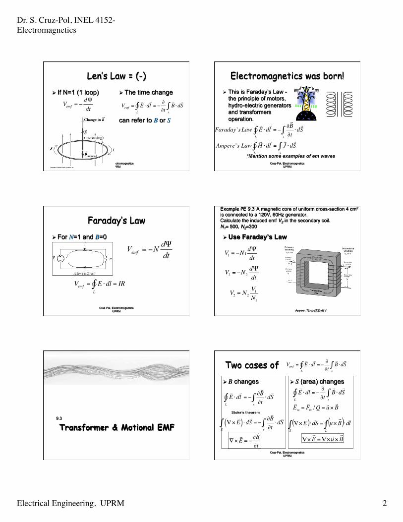
Len’s Law = (-) Ø  If N=1 (1 loop) Ø The time change

can refer to B or S


Vemf = −dΨdt Vemf =

!E

L"∫ ⋅d

!l = − ∂

∂t!B ⋅d!S

s∫


Electromagnetics was born! Ø  This is Faraday’s Law -

the principle of motors, hydro-electric generators and transformers operation.

*Mention some examples of em waves

Faraday 's Law!E

L"∫ ⋅d

!l = − ∂

!B∂t⋅d!S

s∫

Ampere 's Law!H

L"∫ ⋅d

!l =

!J ⋅d!S

s∫

Faraday’s Law Ø For N=1 and B=0


dtdNVemfΨ

−=

Vemf = EL!∫ ⋅dl = IR

Example PE 9.3 A magnetic core of uniform cross-section 4 cm2 is connected to a 120V, 60Hz generator. Calculate the induced emf V2 in the secondary coil.N1= 500, N2=300#

Ø Use Faraday’s Law

Answer; 72 cos(120πt) V

V1 = −N1dΨdt

V2 = −N2dΨdt

V2 = N2V1N1

Transformer & Motional EMF 9.3

Two cases of Ø B changes Ø S (area) changes


!E

L"∫ ⋅dl = − ∂

∂t!B ⋅d!S

s∫

!Em =

!Fm /Q =

!u ×!B

!E

L"∫ ⋅d

!l = − ∂

!B∂t⋅d!S

s∫

Vemf =!E

L"∫ ⋅d

!l = − ∂

∂t!B ⋅d!S

s∫

∇×!E( )

S∫ ⋅d

!S = − ∂

!B∂t⋅d!S

s∫

∇×!E = −∂

!B∂t

Stoke’s theorem

( ) ( ) dlBudSELS

⋅×=⋅×∇ ∫∫!

BuE!!!

××∇=×∇



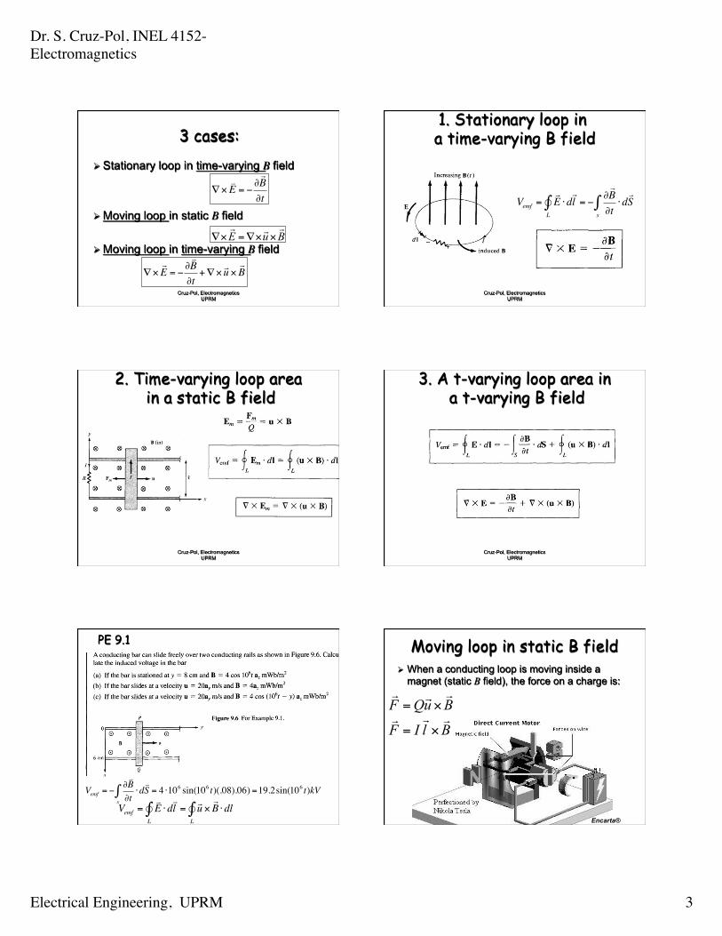
3 cases: Ø Stationary loop in time-varying B field

Ø Moving loop in static B field

Ø Moving loop in time-varying B field


∇×!E = −∂

"B∂t

BuE!!!

××∇=×∇

∇×!E = −∂

"B∂t+∇×

!u ×!B

1. Stationary loop in a time-varying B field


Vemf =!E

L"∫ ⋅d

!l = − ∂

!B∂t⋅d!S

s∫

2. Time-varying loop area in a static B field


3. A t-varying loop area in a t-varying B field


PE 9.1

Vemf = −∂!B∂t⋅d!S

s∫ = 4 ⋅106 sin(106 t)(.08).06) =19.2sin(106 t)kV

Vemf =!E

L"∫ ⋅d

!l = #u ×

#B ⋅dl

L"∫ Cruz-Pol, Electromagnetics

UPRM

Moving loop in static B field Ø  When a conducting loop is moving inside a

magnet (static B field), the force on a charge is:

BlIF

BuQF!!!

!!!

×=

×=

Encarta®



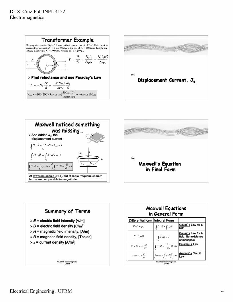
Transformer Example


Ø Find reluctance and use Faraday’s Law

Vemf = −100(200)(3ω cosωt)500µo10

−3

2π (0.10)= −6π cos100π t

Displacement Current, Jd

9.4


Maxwell noticed something was missing…

Ø  And added Jd, the displacement current

IIdSJdlH encSL

==⋅=⋅ ∫∫1

02

=⋅=⋅ ∫∫SL

dSJdlHI

S2

S1

L

IdtdQdSD

dtddSJdlH

SSd

L

==⋅=⋅=⋅ ∫∫∫22

At low frequencies J>>Jd, but at radio frequencies both terms are comparable in magnitude.

Maxwell’s Equation in Final Form

9.4


Summary of Terms Ø E = electric field intensity [V/m] Ø D = electric field density [C/m2] Ø H = magnetic field intensity, [A/m] Ø B = magnetic field density, [Teslas] Ø J = current density [A/m2]


Maxwell Equations in General Form

Differential form Integral Form Gauss’s Law for E field.

Gauss’s Law for H field. Nonexistence of monopole Faraday’s Law

Ampere’s Circuit Law

vD ρ=⋅∇

0=⋅∇ B

tBE∂

∂−=×∇

tDJH∂∂

+=×∇

∫∫ =⋅v

vs

dvdSD ρ

0=⋅∫s

dSB

∫∫ ⋅∂

∂−=⋅

sL

dSBt

dlE

∫∫ ⋅⎟⎠

⎞⎜⎝

⎛∂

∂+=⋅

sL

dStDJdlH




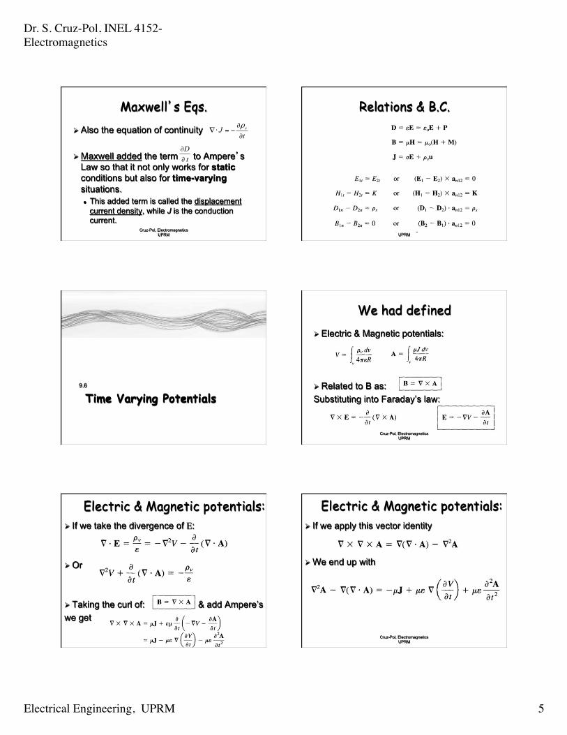
Maxwell’s Eqs. Ø Also the equation of continuity

Ø Maxwell added the term to Ampere’s Law so that it not only works for static conditions but also for time-varying situations. l  This added term is called the displacement

current density, while J is the conduction current.

tJ v

∂

∂−=⋅∇

ρ

tD∂∂

Relations & B.C.


Time Varying Potentials 9.6

We had defined Ø Electric & Magnetic potentials:

Ø Related to B as: Substituting into Faraday’s law:


Electric & Magnetic potentials: Ø  If we take the divergence of E:

Ø Or

Ø Taking the curl of: & add Ampere’s we get


Electric & Magnetic potentials: Ø  If we apply this vector identity

Ø We end up with




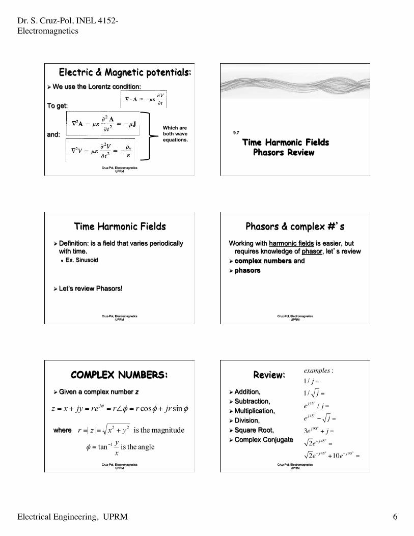
Electric & Magnetic potentials: Ø We use the Lorentz condition:

To get: and:


Which are both wave equations. Time Harmonic Fields

Phasors Review

9.7

Time Harmonic Fields Ø Definition: is a field that varies periodically

with time. l  Ex. Sinusoid

Ø Let’s review Phasors!



Phasors & complex #’s Working with harmonic fields is easier, but

requires knowledge of phasor, let’s review Ø complex numbers and Ø phasors


COMPLEX NUMBERS: Ø Given a complex number z

where

φφφφ sincos jrrrrejyxz j +=∠==+=

magnitude theis || 22 yxzr +==

angle theis tan 1

xy−=φ


Review: Ø Addition, Ø Subtraction, Ø Multiplication, Ø Division, Ø Square Root, Ø Complex Conjugate

examples :1 / j =

1/ j =

e j45o

/ j =

e j45o

− j =

3e j90o

+ j =

2e+ j45o

=

2e+ j45o

+10e+ j90o

=




For a Time-varying phase

Real and imaginary parts are:

φ =ωt +θ

Re{re jφ}= rcos(ωt +θ )

Im{re jφ}= rsin(ωt +θ )


PHASORS Ø For a sinusoidal current equals the real part of

I(t) = Io cos(ωt +θ )tjj

o eeI ωθ

θjoeI

tje ω

sI

Ø The complex term which results from dropping the time factor is called the phasor current, denoted by (s comes from sinusoidal)


To change back to time domain The phasor is 1.  multiplied by the time factor, e jωt, 2.  and taken the real part.

}Re{ tjseAA ω=


Advantages of phasors Ø Time derivative in time is equivalent to

multiplying its phasor by jω

Ø Time integral is equivalent to dividing by the same term.

sAjtA

ω→∂

∂

ωjA

tA s→∂∫

Time Harmonic Fields 9.7


Time-Harmonic fields (sines and cosines)

Ø The wave equation can be derived from Maxwell equations, indicating that the changes in the fields behave as a wave, called an electromagnetic wave or field.

Ø Since any periodic wave can be represented as a sum of sines and cosines (using Fourier), then we can deal only with harmonic fields to simplify the equations.




tDJH∂∂

+=×∇

tBE∂

∂−=×∇

0=⋅∇ B

vD ρ=⋅∇

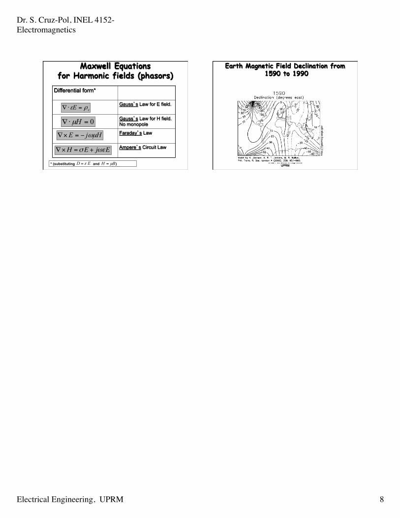
Maxwell Equations for Harmonic fields (phasors)

Differential form*

Gauss’s Law for E field.

Gauss’s Law for H field. No monopole

Faraday’s Law

Ampere’s Circuit Law

vE ρε =⋅∇

0=⋅∇ Hµ

HjE ωµ−=×∇

∇×H =σE + jωεE

* (substituting and ) ED ε= BH µ=

Earth Magnetic Field Declination from 1590 to 1990


Documents

Stationary Charges Electromagnetism E Magnetostatic fields ...ece.uprm.edu/~pol/pdf/MaxEq.pdf · Ø Stationary Charges ... currents l I(t) Ø Electrostatic fields\ E Magnetostatic