Embed Size (px)
Citation preview
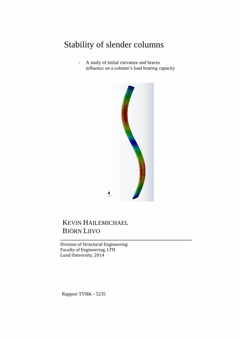
Stability of slender columns
- A study of initial curvature and braces
influence on a column’s load bearing capacity
KEVIN HAILEMICHAEL
BJÖRN LIIVO
Division of Structural Engineering Faculty of Engineering, LTH Lund University, 2014
Rapport TVBK - 5235
Avdelningen för Konstruktionsteknik Lunds Tekniska Högskola
Box 118
221 00 LUND
Division of Structural Engineering Faculty of Engineering, LTH
P.O. Box 118
S-221 00 LUND
Sweden
Stability of slender columns
- A study of initial curvature and braces influence on a column’s load
bearing capacity
Kevin Hailemichael
Björn Liivo
September, 2014
Rapport TVBK-5235 ISSN 0349-4969 ISRN: LUTVDG/TVBK-14/5235+(63)
Master Thesis
Supervisors: Anders Klasson, PhD student Eva Frühwald Hansson, Assistant Professor Division of Structural Engineering
Examiner Roberto Crocetti, Professor Division of Structural Engineering
September 2014
Abstract
Failures due to instability phenomena will happen suddenly and can cause the whole
structure to collapse. It’s therefore in the engineer’s best interest to have a good knowledge
about these phenomena. One example of instability phenomena is column buckling, which
is the main focus of this thesis.
The main cases that are being evaluated have a single brace in the middle of a timber
column with hinged ends, where a part of the report revolves around a comparison of
calculation methods for column buckling in Eurocode and the U.S. Building code.
The second part revolves around the influence of the initial curvature shape and magnitude
on a column. During this evaluation second order is taken into account in the numerical
analysis. Finally the brace stiffness and reaction force on a column is evaluated, to gain a
better understanding of its overall influence on a column’s load bearing capacity.
In the study it was shown that Eurocode and the U.S. Building code weren’t comparable
due to formation of respective building code. A comparison between the two building codes
was however done, to get a better understanding of the difference between the two.
Results show that a larger initial curvature leads to a larger reduction to the overall load
bearing capacity for a column. The assumed shape of the initial curvature has a large
impact on the load bearing capacity. There exist a large discrepancy between the simplified
shape of the initial curvature and the least beneficial, which depends on the size and shape
of the initial curvature.
Findings show that an increase of a column’s brace stiffness contributes to the load bearing
capacity even though the stiffness might be small. The European standard however
demands a minimum stiffness for a brace to be considered acceptable.
The study also shows that the brace force is dependent on the initial curvature of the
column and the bracing stiffness. Yura’s & Helwig’s brace force expression is studied and
compared with the result of a numerical analysis.
Keywords: Column buckling, bracing, building codes, stiffness, initial curvature,
imperfection

Acknowledgements
This master thesis is written for the Civil Engineering program, with the specialization in
Structural Engineering, for the Division of Structural Engineering at Lund University,
Faculty of Engineering.
We would like to take this opportunity to thank all people that have contributed and helped
us during this process. We would especially want to thank our supervisors, PhD student
Anders Klasson and assistant Professor Eva Frühwald Hansson at the Division of Structural
Engineering, for their support and guidance throughout this thesis.
We would also like to thank friends and family for the support and help during this journey
of ours.
Lund, September 2014
Kevin Hailemichael Björn Liivo
Table of contents
Nomenclature ...................................................................................... 1
1 Introduction ...................................................................................... 3
1.1 Background ................................................................................ 3
1.2 Objectives and aim .................................................................... 3
1.3 Scope .......................................................................................... 4
1.4 Method ........................................................................................ 4
1.5 Outline of this thesis ................................................................. 5
2 Literature review .............................................................................. 7
2.1 Material properties .................................................................... 7
2.1.1 Timber ................................................................................... 7
2.2 Stability theory ........................................................................... 8
2.3 Failure due to geometry ............................................................ 9
2.3.1 Buckling .............................................................................. 10
2.4 Bracing of columns ................................................................. 10
2.4.1 Bracing at the end of a column element .............................. 11
2.4.2 Bracing at the middle of a column element ......................... 13
2.4.2.1 Imperfections ................................................................ 16
2.4.2.2 Brace force ................................................................... 17
3 Standards and building codes ...................................................... 19
3.1 Theoretical members opposed to real members .................. 19
3.2 Design according to Eurocode 5 ............................................ 20
3.2.1 Column Subjected to Compression..................................... 20
3.2.2 Live loads in Eurocode ........................................................ 22
3.2.3 Single members in compression ......................................... 22
3.3 Design according to the U.S. standard .................................. 22
3.3.1 Axially loaded column ......................................................... 22
3.3.2 Live loads in U.S. Building code ......................................... 25
3.4 Finite Element Method and modeling .................................... 25
3.4.1 Mathematical modeling ....................................................... 26
3.4.1.1 First order theory .......................................................... 26
3.4.1.2 Second order theory ..................................................... 26
3.4.1.3 Third order theory ......................................................... 26
4 Modeling ......................................................................................... 27
4.1 Case study ............................................................................... 27
4.1.1 Material properties .............................................................. 27
4.2 Finite Element Method (FEM) model ...................................... 28
4.2.1 Geometry ............................................................................ 28
4.2.2 Load case ........................................................................... 28
4.2.3 Boundary conditions ........................................................... 28
4.2.4 Mesh .................................................................................... 29
4.2.5 Linear perturbation buckle analysis ..................................... 29
4.2.6 Second order analysis ......................................................... 30
4.3 Comparison between the building codes .............................. 30
4.3.1 According to Eurocode 5 ..................................................... 30
4.3.2 According to the U.S. standard ............................................ 31
4.4 Initial curvature ........................................................................ 32
4.4.1 Critical force dependency to initial curvature ....................... 32
4.4.2 Shape and magnitude of Initial curvature in a column ......... 32
4.5 Bracing of a column ................................................................. 34
4.5.1 Ideal stiffness according to Yura ......................................... 34
4.5.2 Bracing stiffness in Eurocode .............................................. 34
4.5.3 Stiffness of a brace .............................................................. 34
4.5.4 Influence of several braces .................................................. 34
4.5.5 Brace force study................................................................. 35
4.5.6 Influence of initial curvature ................................................. 35
5 Results and Discussion ................................................................. 37
5.1 Comparison between different building codes ..................... 37
5.1.1 Eurocode and the U.S. Building code .................................. 37
5.1.2 Analysis of results................................................................ 38
5.2 Initial curvatures effect on the load bearing capacity .......... 38
5.2.1 Effect of initial curvature ...................................................... 38
5.2.2 Critical force dependency due to initial curvature ................ 39
5.2.3 Shape and magnitude of initial curvature ............................ 41
5.2.4 Analysis of results................................................................ 44
5.3 Stiffness requirement of a brace ............................................ 45
5.3.1 Yura’s and Helwig’s model .................................................. 45
5.3.2 Eurocode’s stiffness requirement ........................................ 47
5.3.3 Influence of several braces .................................................. 47
5.3.4 Analysis of results................................................................ 51
5.4 Brace force ............................................................................... 52
5.4.1 Yura’s & Helwig’s model ...................................................... 52
5.4.2 Brace force due to imperfections ......................................... 53
5.4.3 Influence of initial curvature for the brace force ................... 54
5.4.4 Analysis of results................................................................ 55
6 Discussion and Conclusions ......................................................... 57
7 References ...................................................................................... 61
Appendix A - Unit converter
1
Nomenclature
Abbrevations
Eurocode 5 SS-EN 1995-1
FEM Finite Element Method
Latin upper case letters
A Area [m2] or [inch
2]
Load duration factor
Wet service factor
Temperature factor
Size factor
Column stability factor
Inscised factor for sawn lumber
E Young’s modulus [Pa] or [psi]
Modulus of elasticity associated with the axis of column
buckling [Pa]
Modulus of elasticity associated with the axis of olumn buckling
[psi]
F Force [N]
Tabulated compressive stress parallel to grain [psi]
The Euler critical buckling stress for columns [psi]
The design load for the compressive stress parallel to the grain
[psi]
Tabulated compressive stress parallel to grain multiplied by all
adjustment factors except [psi]
I Moment of inertia [m4]
0,3 for visually graded lumber
Effective length factor
L Length [m]
M Moment [Nm]
N Normal force [N]
Nd The design load [N]
P Force [N]
Pcr Critical force [N]
W Section modulus [m3]
Latin lower case letters
b Width [m] or [inch]
h Height [m] or [inch]
c The buckling and crushing interaction factor for columns
Compressive stress capacity parallel to the grain [Pa]
fck Compressive stress capacity parallel to the grain [Pa]
the compressive stress parallel to the grain [psi]
i Gyration ratio
k Brace stiffness [N/m]
2
kc Reduction factor
kideal Ideal brace stiffness [N/m]
kreq The required brace stiffness to prevent side sway [N/m]
l Effective length [m]
Greek lower case letters
β Euler’s buckling factor
Straightness requirement factor
σ Stress [Pa]
λ Slenderness ratio
Relative slenderness ratio
3
1 Introduction
This chapter is an introduction to this report, where the underlying background and the
objective for this report will be given. The chapter starts with an introduction to the
subject, were the problem formulation of the report will be presented. Later in this chapter,
the reader will get more detailed description about the objective and the method of the
report.
1.1 Background
When instability phenomena occurs in a structure the consequences can become dire fast
(Bauchau & Craig, 2009). Failures due to instability phenomena can happen suddenly and
can cause the whole structure to collapse. It’s therefore in the engineer’s best interest to
have a good knowledge about these phenomena. Examples of instability phenomena are
local buckling, column buckling and lateral torsional buckling.
Instability problems such as column buckling can be counteracted by bracing. When
bracing a column for column buckling the brace reduces the effective length of the column,
thus increases the load bearing capacity for the structure and it becomes more stable.
During the design of a brace, the bracing is normally considered to be infinitely stiff to
enforce a certain kind of failure. However an infinitely stiff bracing is never the case in
reality.
However it’s hard to calculate the stiffness for the bracing and the way it’s calculated
differs dependent on the method. It is therefore of importance to gain a better understanding
of how a brace influences the column buckling phenomenon.
1.2 Objectives and aim
Calculation methods to design a column due to column buckling vary between the different
building codes. In this report the difference between how the European and the U.S.
building code calculates the design load for a column in compression are presented. The
design loads is compared to each other and a numerical analysis.
The second part of this thesis is a parametric study where the effects of initial curvature on
the critical load bearing capacity are evaluated. During this evaluation a numerical analysis
is performed to take into account non linearity.
By bracing a column, column buckling can be prevented by increasing the columns load
bearing capacity. It is however hard to evaluate what kind of stiffness properties that is
required for obtaining an effective brace for a wooden column. It is also hard to anticipate
the magnitude of the reaction force in the brace.
Aim
How does the design procedure and results differ between Eurocode and the U.S.
building code, when it comes to timber columns in compression?
4
How does the shape and magnitude of initial curvature influence the load bearing
capacity of a column?
How does the stiffness of a brace affect the load bearing capacity in the column and
the resulting force in the brace? And how does the influence of several braces with
different stiffness affect the load bearing capacity of a column?
1.3 Scope
This thesis focuses on column buckling. The main cases that are being evaluated have a
single brace in the middle of the column with hinged ends. The study will revolve around
timber columns.
The columns that are being evaluated for timber have a rectangular cross-section with the
material properties of timber class c27.
During calculations eccentricities, residual stresses and inclination are not taken into
account unless assigned a specific value. Other deciding factors such as long time
deformations, moisture content for the columns are not considered. While comparing
European with the U.S. building code only calculations with critical load due to column
buckling are done.
The evaluation of a brace’s contribution to the load bearing capacity will only be done in a
linear analysis in FEM. This report evaluates the phenomena up to the second order (by
using computer modeling), this means that no larger deformations are taken into account.
1.4 Method
A literature review of current and relevant knowledge of stability phenomena will be the
base foundation of this report. The procedure of the literature review will be done
analytically and systematically.
To quantify and clarify the relations mentioned in the literature review, a calculation part
will be carried out in the report. These calculations will be based on the European and the
U.S. building codes for structural design and computer model in Brigade.
The European building code for timber is based on SS-EN 1995-1, also called Eurocode 5.
The basis of the European building code for this report comes from the book
“Byggkonstruktion – Regel och formelsamling” by Isaksson and Mårtensson (2010).
The review of the U.S. building code in this report revolves around the book “Design of
Wood Structures – ASD” by Breyer et al (2003). The book goes through the basis for
structural design and includes practical literature. The literature includes publication and
design criteria’s of the National Design Specification for Wood Construction (NDS),
Allowable Stress Design Manual for Engineered Wood Construction and the International
Building Code.
5
Brigade/plus 5.1-4 is an add on program from Scanscot Technology AB to Abaqus from
Dassault Systèmes, that offers a variety of extra features in design of bridges. Brigade is the
preferred and used finite element program for this report, this since it has all the right
properties needed to do advanced calculations but also because the authors are used to its
interface. The finite element method is necessary in this case to obtain the second order and
also used as a comparison to the hand calculations.
1.5 Outline of this thesis
Chapter 1 – Introduction, introduces the problem studied in this report
Chapter 2 – Literature review, underlying theory that serves as a foundation for the report
Chapter 3 – Standards and building codes, presents theory and methods behind the
different standards and building codes
Chapter 4 – Modeling, this part walks through how the calculations and studies are
performed in this report.
Chapter 5 – Results and analysis, presents a results and discussion part, where the
calculations and findings are analyzed and discussed.
Chapter 6 - Discussion and conclusion, a conclusion of the result and discussion is done
to answer the objectives of the report.

6
7
2 Literature review
This chapter is a literature review, where the underlying theory for the report will be
presented. The chapter begins with a short review of the materials that are studied, and
then to describe the theory behind stability theory and the column buckling phenomena. In
connection to the column buckling part, there’ll be a section that describes the influence of
bracing.
2.1 Material properties
In this subchapter general information about the materials wood and steel are presented
from a structural point of view.
2.1.1 Timber Timber comes in all shapes and sizes, since it’s organic it varies in quality. Many of the
weaknesses of wood comes from its growth deviations such as knots, bark that grows
inwards or tree sap (Burström, 2007). The woods anisotropic properties will cause the wood
to absorb moisture differently in each direction. The moisture levels in newly cut timber are
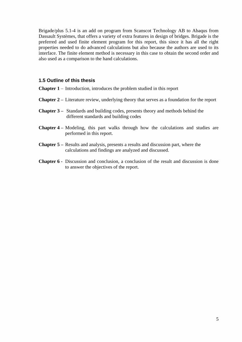
approximately 30-35% at the core (Burström, 2007). When the wood planks later dry out
they will shrink and bend dependent on where they are cut out of the timber log. To
illustrate this see picture 2.1 below, this initial bending can cause irregularities when used.
Figure 2.1 Shapes of dried out wood planks (Burström, 2007)
The strength properties of wood is very complex due to its anisotropic structure (Burström,
2007). Most types of timber have the largest strength capacity when it is subjected to pure
tensile force along the fibers. The lowest strength capacity is obtained when timber is
subjected to pure compressive force along the fibers. Since bending is something in
between the strength will also be something in between tensile and compression strength.
Since wood is anisotropic its strength capacity also becomes dependent on how the wooden
fibers are take on the load. The tensile- and compressive strengths are at a high point when
the wood takes on load parallel to the wooden fibers and noticeably weaker perpendicular
to the same fibers. If the load is applied perpendicular to the wooden fibers the largest
8
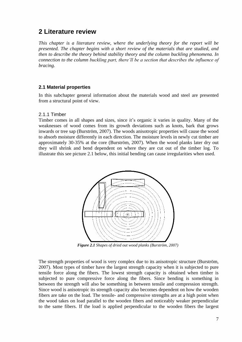
strength is reached parallel to the annual rings of the timber, even known as the tangential
direction. For further viewing of how the three main directions are defined see figure 2.2
below.
Fiber direction (along the trunk)
Radial direction (perpendicular towards the annual rings and the fiber direction)
Tangential direction (perpendicular the fiber direction but parallel towards the
annual rings)
Figure 2.2 The timbers main directions F- fiber, R-radial and T-tangential
The strength properties of wood are directly dependent on the on density, moisture content,
fiber direction, temperature and dimensions (Burström, 2007).
2.2 Stability theory
In the world of mechanics one separates different equilibrium states from each other
(Höglund, 2006). This is done by classifying certain types of scenarios into three main
categories,
Stable
Unstable
Neutral
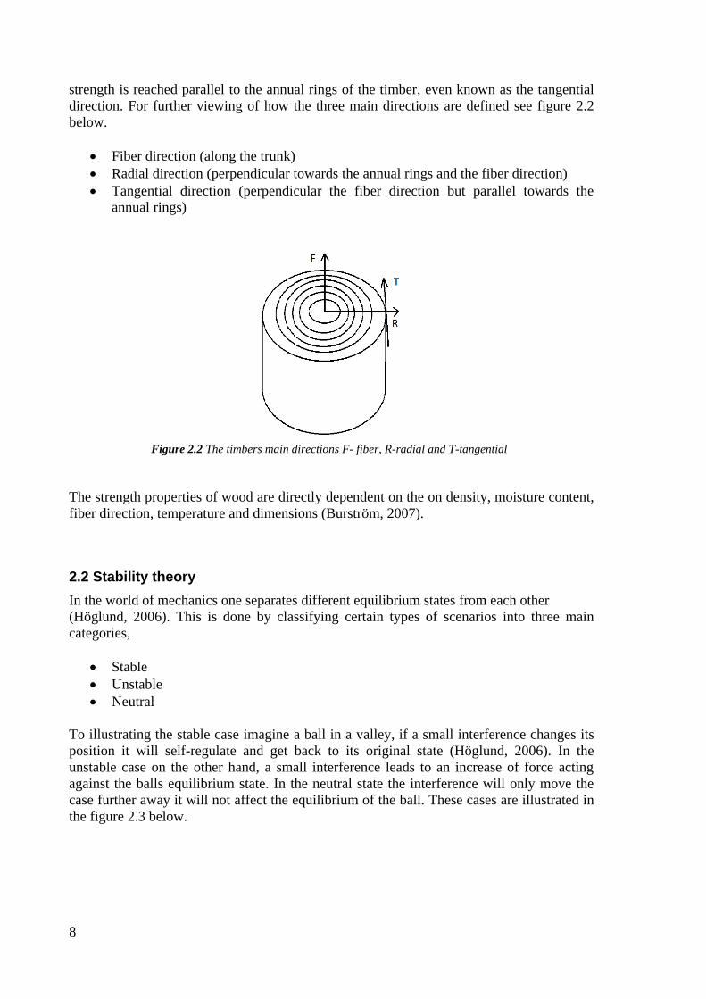
To illustrating the stable case imagine a ball in a valley, if a small interference changes its
position it will self-regulate and get back to its original state (Höglund, 2006). In the
unstable case on the other hand, a small interference leads to an increase of force acting
against the balls equilibrium state. In the neutral state the interference will only move the
case further away it will not affect the equilibrium of the ball. These cases are illustrated in
the figure 2.3 below.
9
Figure 2.3 Stability cases, from left to right stable, unstable and neutral (Höglund, 2006)
Preconditions for a body are the determining factor in how the body will act when it’s
subjected to a load (Höglund, 2006). Thus one can say that a structure is in a stable
equilibrium if it will self-regulate back to its original position after exposure to a small
interference. While examining stability phenomena one often presume certain restrictions
for instance,
Material properties are linear elastic
The shape of the structural element has an ideal form
Constitutive properties are based on presumptions of small deformations
Dependent on what kind of mechanical phenomena that occurs on the load bearing structure
different failure modes can occur (Höglund, 2006). If a structure is subjected to tensile
forces the material yield strength, fatigue or breaking point becomes critical for failure.
However compressive forces enforce column buckling or local buckling to take precedence
above other parameters concerning failure for slender columns.
2.3 Failure due to geometry
Depending on the column’s geometry, the allowable stress for a given material can vary
and be divided into three groups (Efunda, 2014). The three groups are the short,
intermediate and long column.
The materials strength limit is the dominating factor for a short column. For an intermediate
respective a long column it’s however the inelastic and the elastic limit that are the
bounding factor for the column members (Efunda, 2014). The slenderness or the stiffness of
the column becomes more and more important as a column becomes longer. The capacity
of the material in a column, that is long and slender, will not be fully utilized. The column
will buckle before the stresses in the column reaches the stress limit of the material.
For an illustration of the correlation between the strength limit and the slenderness ratio for
the different groups, see figure 2.4 below.
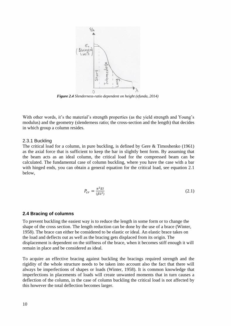
10
Figure 2.4 Slenderness-ratio dependent on height (efunda, 2014)
With other words, it’s the material’s strength properties (as the yield strength and Young’s
modulus) and the geometry (slenderness ratio; the cross-section and the length) that decides
in which group a column resides.
2.3.1 Buckling The critical load for a column, in pure buckling, is defined by Gere & Timoshenko (1961)
as the axial force that is sufficient to keep the bar in slightly bent form. By assuming that
the beam acts as an ideal column, the critical load for the compressed beam can be
calculated. The fundamental case of column buckling, where you have the case with a bar
with hinged ends, you can obtain a general equation for the critical load, see equation 2.1
below,
(2.1)
2.4 Bracing of columns
To prevent buckling the easiest way is to reduce the length in some form or to change the
shape of the cross section. The length reduction can be done by the use of a brace (Winter,
1958). The brace can either be considered to be elastic or ideal. An elastic brace takes on
the load and deflects out as well as the bracing gets displaced from its origin. The
displacement is dependent on the stiffness of the brace, when it becomes stiff enough it will
remain in place and be considered as ideal.
To acquire an effective bracing against buckling the bracings required strength and the
rigidity of the whole structure needs to be taken into account also the fact that there will
always be imperfections of shapes or loads (Winter, 1958). It is common knowledge that
imperfections in placements of loads will create unwanted moments that in turn causes a
deflection of the column, in the case of column buckling the critical load is not affected by
this however the total deflection becomes larger.

11
2.4.1 Bracing at the end of a column element If a column is subjected to an axial load, hinged on the ends with the assumption of
adequate stiffness to the restraints, the critical load is given by Euler’s load (Helwig &
Yura, 1996). For illustration for the case, see figure 2.5 and equation 2.2 below,
Figure 2.5 Hinged and braced top of a column (Helwig &Yura, 1996)
(2.2)
Consider now that the top end is elastic and that the bracing is inadequate, this will result in
the inevitable deflection of the column but also a displacement of the bracings original
position, see figure 2.6 below.
Figure 2.6 Inadequate stiffness gives side sway (Helwig &Yura, 1996)
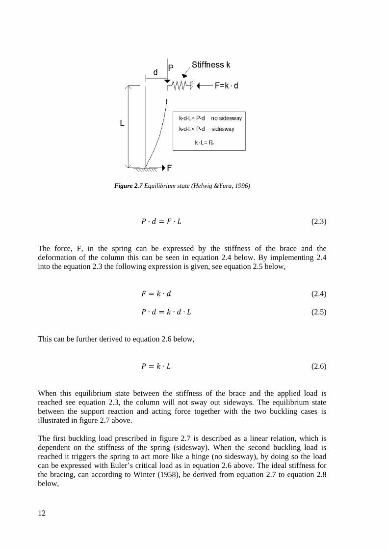
The manner of which the structure acts can be described by the moment equilibrium state at
the hinge. The expression of the equilibrium can according to Helwig & Yura (1996) be
illustrated and expressed by figure 2.7 and equation 2.3 below,
12
Figure 2.7 Equilibrium state (Helwig &Yura, 1996)
(2.3)
The force, F, in the spring can be expressed by the stiffness of the brace and the
deformation of the column this can be seen in equation 2.4 below. By implementing 2.4
into the equation 2.3 the following expression is given, see equation 2.5 below,
(2.4)
(2.5)
This can be further derived to equation 2.6 below,
(2.6)
When this equilibrium state between the stiffness of the brace and the applied load is
reached see equation 2.3, the column will not sway out sideways. The equilibrium state
between the support reaction and acting force together with the two buckling cases is
illustrated in figure 2.7 above.
The first buckling load prescribed in figure 2.7 is described as a linear relation, which is
dependent on the stiffness of the spring (sidesway). When the second buckling load is
reached it triggers the spring to act more like a hinge (no sidesway), by doing so the load
can be expressed with Euler’s critical load as in equation 2.6 above. The ideal stiffness for
the bracing, can according to Winter (1958), be derived from equation 2.7 to equation 2.8
below,
13
(2.7)
(2.8)
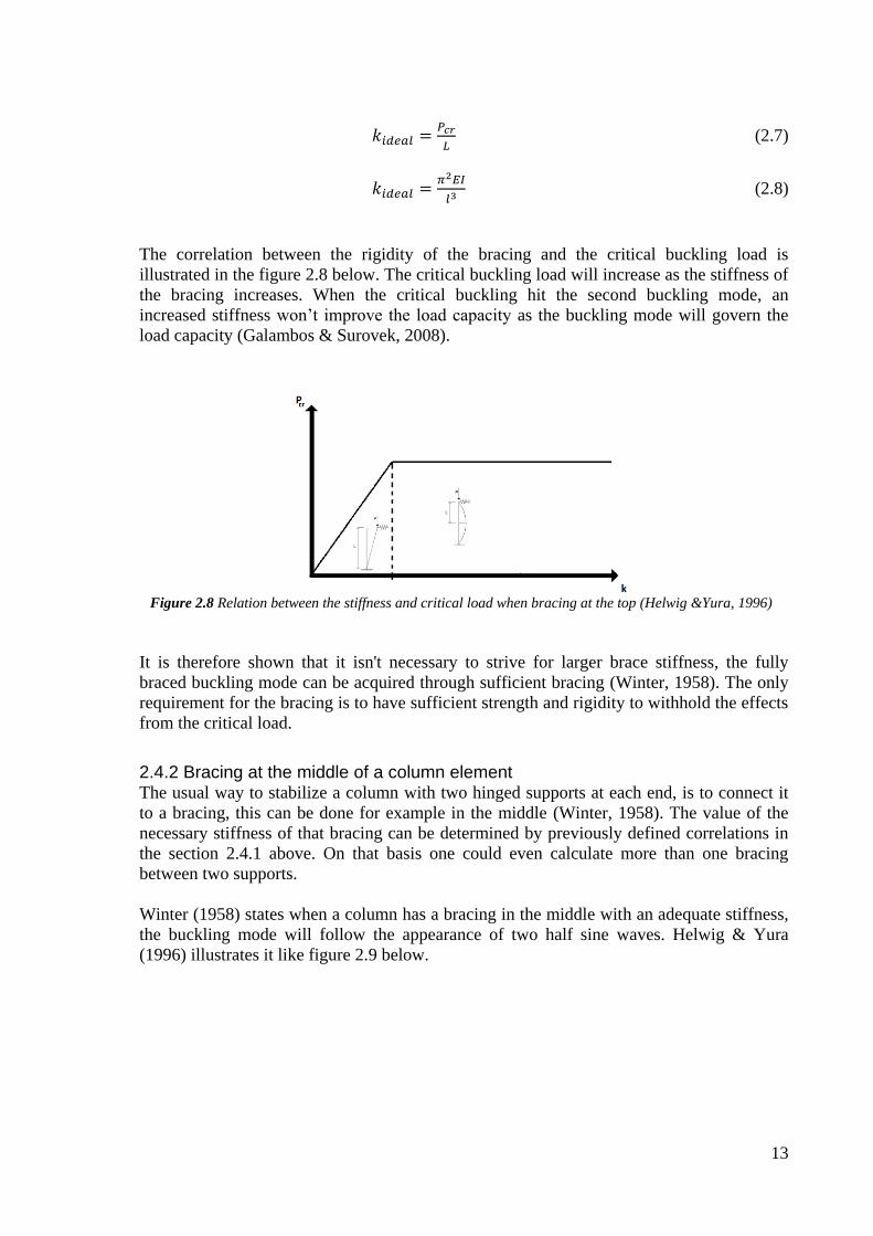
The correlation between the rigidity of the bracing and the critical buckling load is
illustrated in the figure 2.8 below. The critical buckling load will increase as the stiffness of
the bracing increases. When the critical buckling hit the second buckling mode, an
increased stiffness won’t improve the load capacity as the buckling mode will govern the
load capacity (Galambos & Surovek, 2008).
Figure 2.8 Relation between the stiffness and critical load when bracing at the top (Helwig &Yura, 1996)
It is therefore shown that it isn't necessary to strive for larger brace stiffness, the fully
braced buckling mode can be acquired through sufficient bracing (Winter, 1958). The only
requirement for the bracing is to have sufficient strength and rigidity to withhold the effects
from the critical load.
2.4.2 Bracing at the middle of a column element The usual way to stabilize a column with two hinged supports at each end, is to connect it
to a bracing, this can be done for example in the middle (Winter, 1958). The value of the
necessary stiffness of that bracing can be determined by previously defined correlations in
the section 2.4.1 above. On that basis one could even calculate more than one bracing
between two supports.
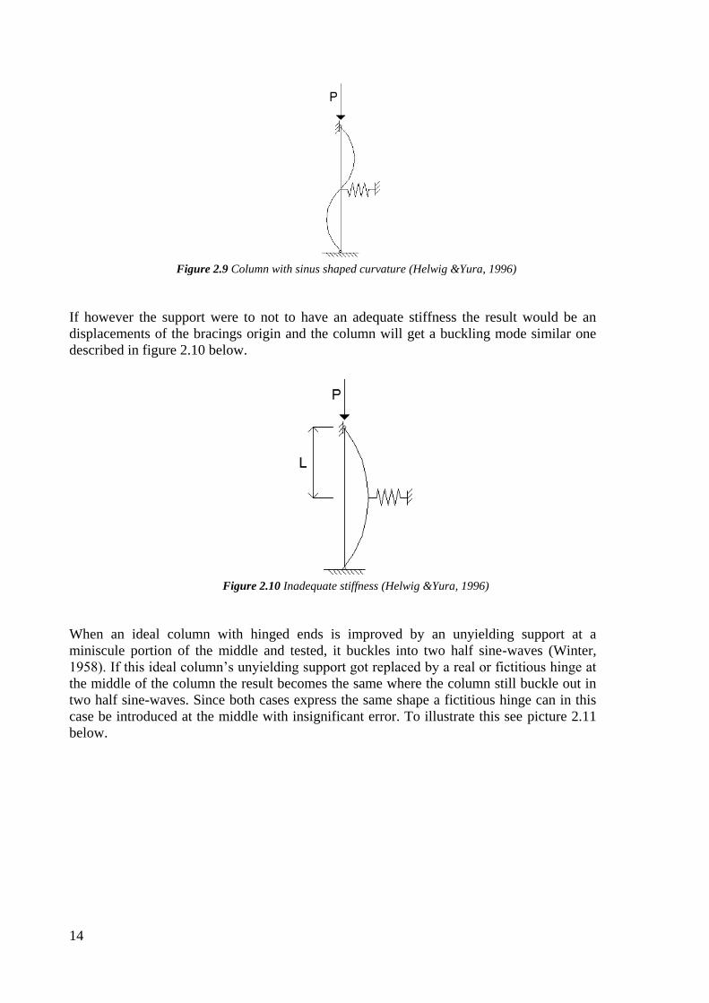
Winter (1958) states when a column has a bracing in the middle with an adequate stiffness,
the buckling mode will follow the appearance of two half sine waves. Helwig & Yura
(1996) illustrates it like figure 2.9 below.
14
Figure 2.9 Column with sinus shaped curvature (Helwig &Yura, 1996)
If however the support were to not to have an adequate stiffness the result would be an
displacements of the bracings origin and the column will get a buckling mode similar one
described in figure 2.10 below.
Figure 2.10 Inadequate stiffness (Helwig &Yura, 1996)
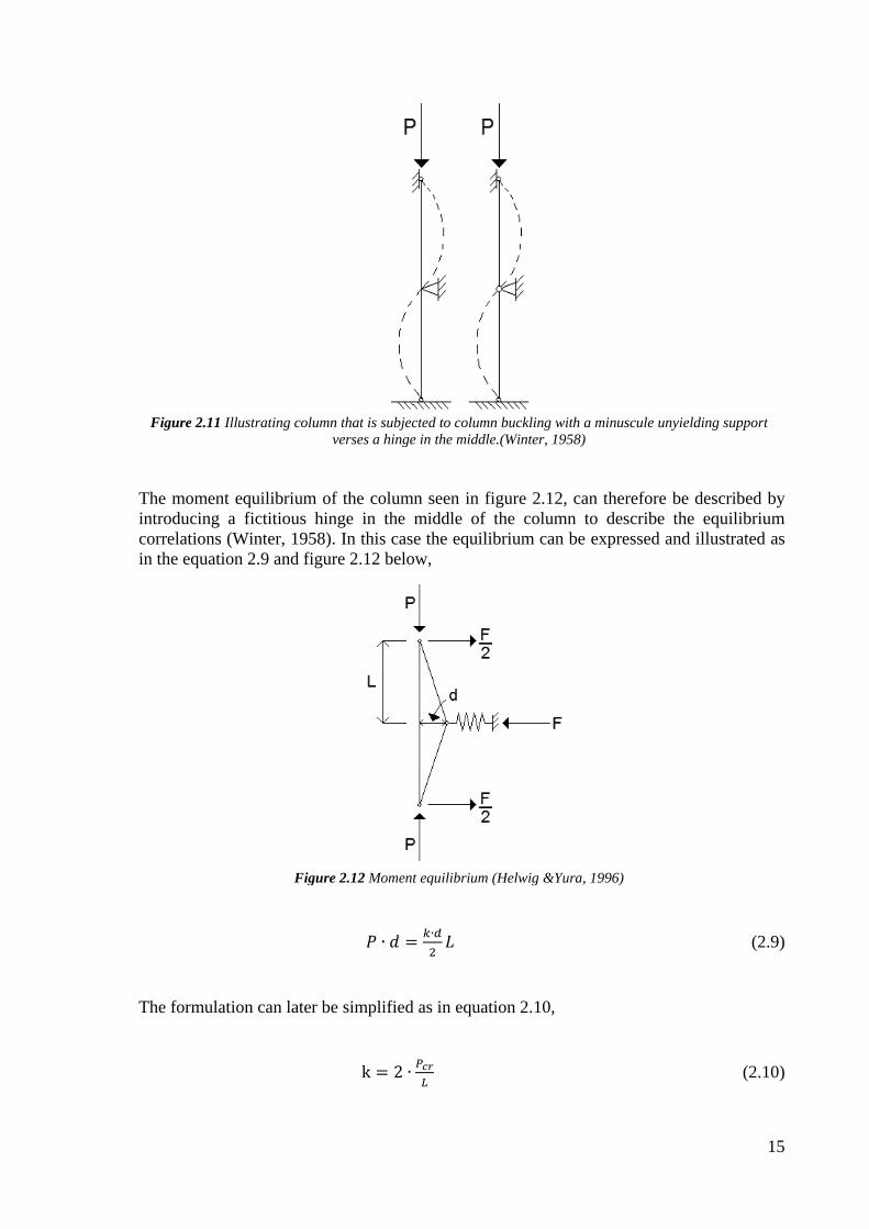
When an ideal column with hinged ends is improved by an unyielding support at a
miniscule portion of the middle and tested, it buckles into two half sine-waves (Winter,
1958). If this ideal column’s unyielding support got replaced by a real or fictitious hinge at
the middle of the column the result becomes the same where the column still buckle out in
two half sine-waves. Since both cases express the same shape a fictitious hinge can in this
case be introduced at the middle with insignificant error. To illustrate this see picture 2.11
below.
15
Figure 2.11 Illustrating column that is subjected to column buckling with a minuscule unyielding support
verses a hinge in the middle.(Winter, 1958)
The moment equilibrium of the column seen in figure 2.12, can therefore be described by
introducing a fictitious hinge in the middle of the column to describe the equilibrium
correlations (Winter, 1958). In this case the equilibrium can be expressed and illustrated as
in the equation 2.9 and figure 2.12 below,
Figure 2.12 Moment equilibrium (Helwig &Yura, 1996)
(2.9)
The formulation can later be simplified as in equation 2.10,
(2.10)
16
Based on this correlation one can later evolve it to the expression in equation 2.11 for the
necessary stiffness for the bracing, , in the same manner as in previous sections,
(2.11)
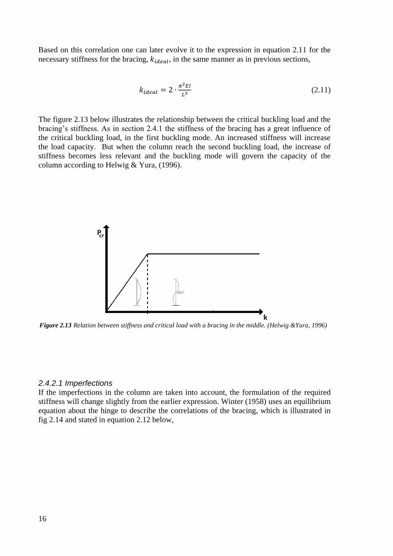
The figure 2.13 below illustrates the relationship between the critical buckling load and the
bracing’s stiffness. As in section 2.4.1 the stiffness of the bracing has a great influence of
the critical buckling load, in the first buckling mode. An increased stiffness will increase
the load capacity. But when the column reach the second buckling load, the increase of
stiffness becomes less relevant and the buckling mode will govern the capacity of the
column according to Helwig & Yura, (1996).
Figure 2.13 Relation between stiffness and critical load with a bracing in the middle. (Helwig &Yura, 1996)
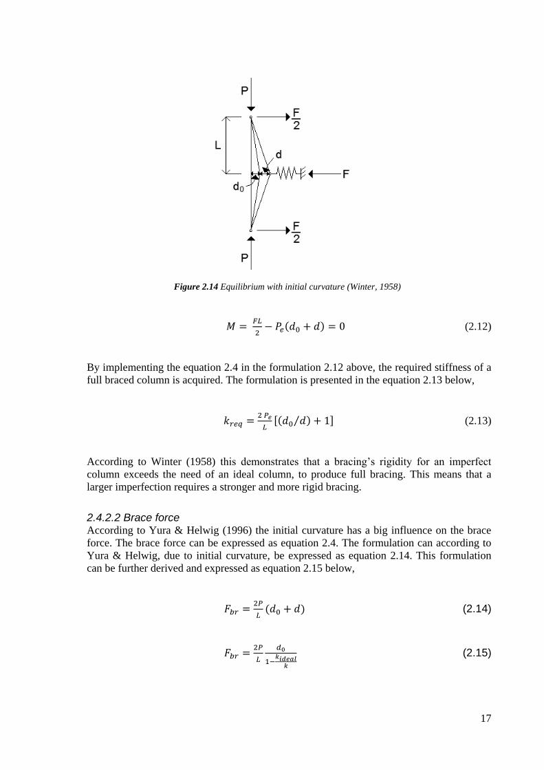
2.4.2.1 Imperfections If the imperfections in the column are taken into account, the formulation of the required
stiffness will change slightly from the earlier expression. Winter (1958) uses an equilibrium
equation about the hinge to describe the correlations of the bracing, which is illustrated in
fig 2.14 and stated in equation 2.12 below,
17
Figure 2.14 Equilibrium with initial curvature (Winter, 1958)
(2.12)
By implementing the equation 2.4 in the formulation 2.12 above, the required stiffness of a
full braced column is acquired. The formulation is presented in the equation 2.13 below,
[ ⁄ ] (2.13)
According to Winter (1958) this demonstrates that a bracing’s rigidity for an imperfect
column exceeds the need of an ideal column, to produce full bracing. This means that a
larger imperfection requires a stronger and more rigid bracing.
2.4.2.2 Brace force According to Yura & Helwig (1996) the initial curvature has a big influence on the brace
force. The brace force can be expressed as equation 2.4. The formulation can according to
Yura & Helwig, due to initial curvature, be expressed as equation 2.14. This formulation
can be further derived and expressed as equation 2.15 below,
(2.14)
(2.15)

18
19
3 Standards and building codes
This chapter is a review of the methods and design standards that are in use in the report.
The chapter starts with an introduction that describes the differences between an ideal- and
a real member. The reader will also get a presentation of the design building codes in
Europe and U.S. for timber columns in compression. A section about the Finite Element
Method (FEM) will later be presented, to describe the method in general.
3.1 Theoretical members opposed to real members
The difference between theoretical and the practical member is the existence of different
unspecified factors that together with the deviation from the linear elastic behavior acts on
the member (Runesson et al., 1992). During design procedures these conditions need to be
taken into account in general, for instance:
Inhomogeneity in material properties
Initial stresses in the form of residual stresses
Initial curvature
Eccentricity of axial load point of application
Real members are never perfectly straight nor are there load applied without eccentricities
(Trahair & Bradford, 1994). To simplify the problem these imperfections can be equal to an
addition in initial curvature since the behavior is similar.
Initial curvature is a form of geometrical imperfection where a straight beam or column has
a natural curvature to its shape often caused by residual stresses (Trahair & Bradford,
1994). The maximum allowed stresses and design rules that takes initial curvature into
account are based on semi-empirical studies. Residual stresses are those stresses that act
internally on a structural member in an unloaded state. By definition this means that those
stresses are in equilibrium since they are there without external forces (Höglund, 2006).
However residual stresses are not being taken into account in this report.
The shape of how the initial curvature acts in a column is very irregular and different in
each case. When the column becomes subjected to a load the buckling effect is added with
the initial curvature and thereby speeds up the process of failure due to column buckling.
The model assumption is that the shape for column buckling also is the shape for the initial
curvature of the column. In this case the total deflection becomes the contribution from the
column buckling and the contribution from the initial curvature.
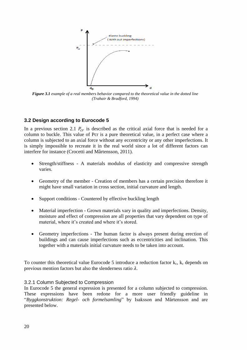
When adding all deviations on a perfect member the critical load is reduced dependent on
how much and of what the actual member is exposed to (Trahair & Bradford, 1994). To
illustrate an example of a real member compared with a purely theoretical member see
figure 3.1 below,
20
Figure 3.1 example of a real members behavior compared to the theoretical value in the dotted line
(Trahair & Bradford, 1994)
3.2 Design according to Eurocode 5
In a previous section 2.1 is described as the critical axial force that is needed for a
column to buckle. This value of Pcr is a pure theoretical value, in a perfect case where a
column is subjected to an axial force without any eccentricity or any other imperfections. It
is simply impossible to recreate it in the real world since a lot of different factors can
interfere for instance (Crocetti and Mårtensson, 2011).
Strength/stiffness - A materials modulus of elasticity and compressive strength
varies.
Geometry of the member - Creation of members has a certain precision therefore it
might have small variation in cross section, initial curvature and length.
Support conditions - Countered by effective buckling length
Material imperfection - Grown materials vary in quality and imperfections. Density,
moisture and effect of compression are all properties that vary dependent on type of
material, where it’s created and where it’s stored.
Geometry imperfections - The human factor is always present during erection of
buildings and can cause imperfections such as eccentricities and inclination. This
together with a materials initial curvature needs to be taken into account.
To counter this theoretical value Eurocode 5 introduce a reduction factor kc, kc depends on
previous mention factors but also the slenderness ratio .
3.2.1 Column Subjected to Compression In Eurocode 5 the general expression is presented for a column subjected to compression.
These expressions have been redone for a more user friendly guideline in
“Byggkonstruktion: Regel- och formelsamling” by Isaksson and Mårtensson and are
presented below.
21
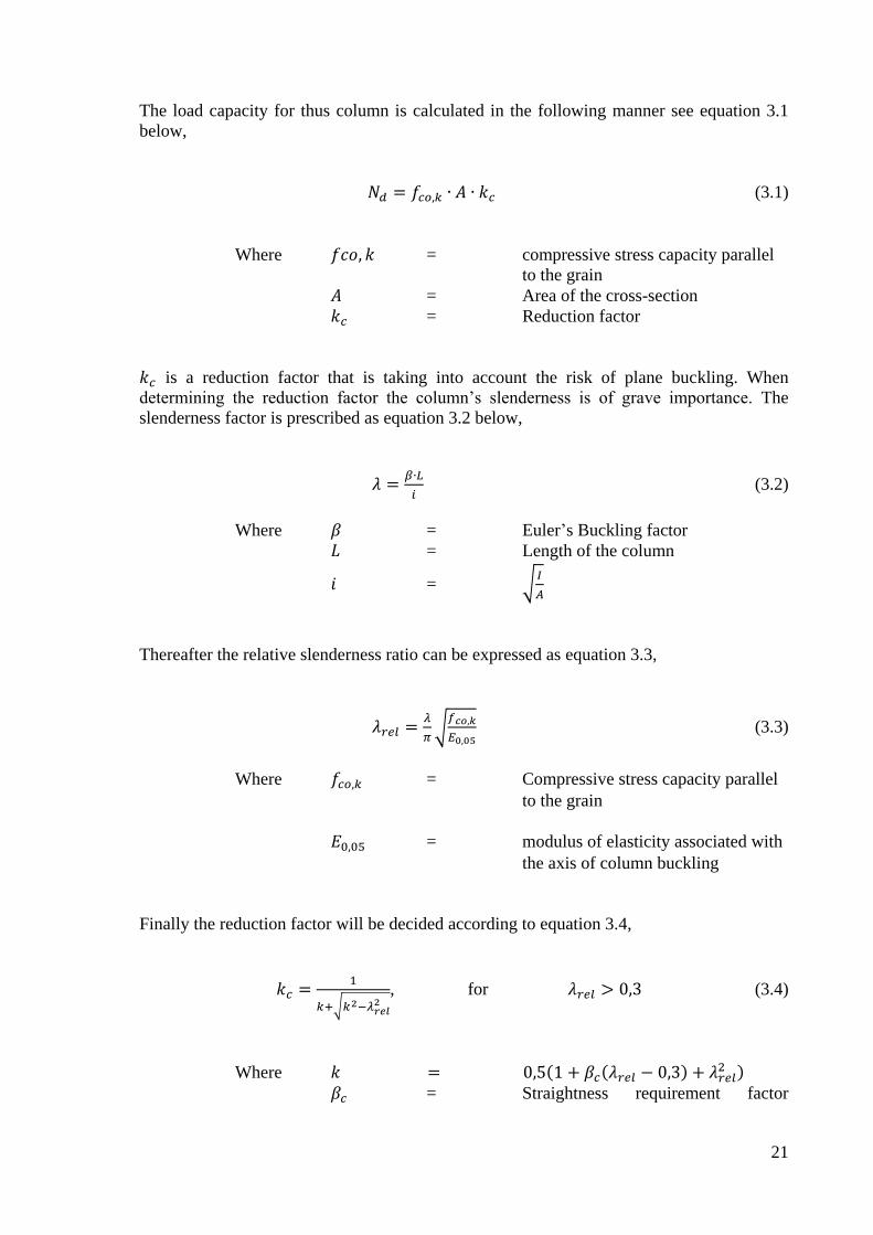
The load capacity for thus column is calculated in the following manner see equation 3.1
below,
(3.1)
Where = compressive stress capacity parallel
to the grain
= Area of the cross-section
= Reduction factor
is a reduction factor that is taking into account the risk of plane buckling. When
determining the reduction factor the column’s slenderness is of grave importance. The
slenderness factor is prescribed as equation 3.2 below,
(3.2)
Where = Euler’s Buckling factor
= Length of the column
= √
Thereafter the relative slenderness ratio can be expressed as equation 3.3,
√
(3.3)
Where = Compressive stress capacity parallel
to the grain
= modulus of elasticity associated with
the axis of column buckling
Finally the reduction factor will be decided according to equation 3.4,
√
, for (3.4)
Where
= Straightness requirement factor
22
Comments:
The reduction factor kc has been determined by large quantity testing (Crocetti and
Mårtensson, 2011). The columns that were tested was picked at random had different
deviations in material properties, geometry and initial curvature. Property values between
different columns were taken in to account for correlation. By studying the tested columns
using second order one could calculate the ultimate load.
3.2.2 Live loads in Eurocode Design guidance on how to design for imposed loads for structural designs, are also given
by Eurocode. The characteristic values are divided in different categories, which indicate
on its occupancy.
The live load that is of an interest in this report is,
School, classroom:
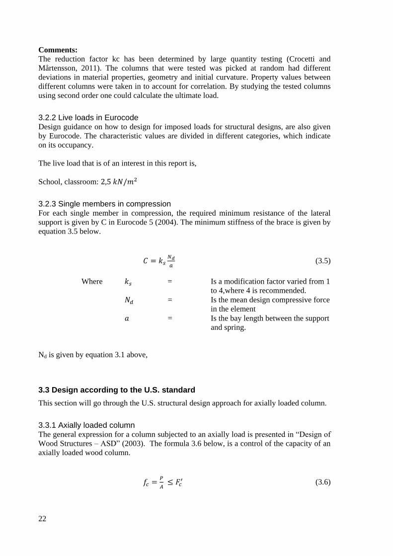
3.2.3 Single members in compression For each single member in compression, the required minimum resistance of the lateral
support is given by C in Eurocode 5 (2004). The minimum stiffness of the brace is given by
equation 3.5 below.
(3.5)
Where = Is a modification factor varied from 1
to 4,where 4 is recommended.
= Is the mean design compressive force
in the element
= Is the bay length between the support
and spring.
Nd is given by equation 3.1 above,
3.3 Design according to the U.S. standard
This section will go through the U.S. structural design approach for axially loaded column.
3.3.1 Axially loaded column The general expression for a column subjected to an axially load is presented in “Design of
Wood Structures – ASD” (2003). The formula 3.6 below, is a control of the capacity of an
axially loaded wood column.
(3.6)
23
Where = the compressive stress parallel to the
grain
P = the members axial compressive force
A = the area of the cross-section
= the design load for the compressive
stress parallel to the grain
The design load is taking in to account several different factors in addition to the column
stability. Example of the different factors is the temperature, the moisture content in wood
and the load duration. The different factors are manifested as adjustment factors.
The formula for the allowable stress in a column is presented in equation 3.7 below.
(3.7)
Where = allowable load for the compressive
stress parallel to the grain
= tabulated compressive stress
parallel to grain
= load duration factor
= wet service factor
= temperature factor
= size factor
= column stability factor
= incised factor for sawn lumber
More detailed information about the various adjustment factors can be found in the book
“Design of Wood Structures – ASD” (2003).
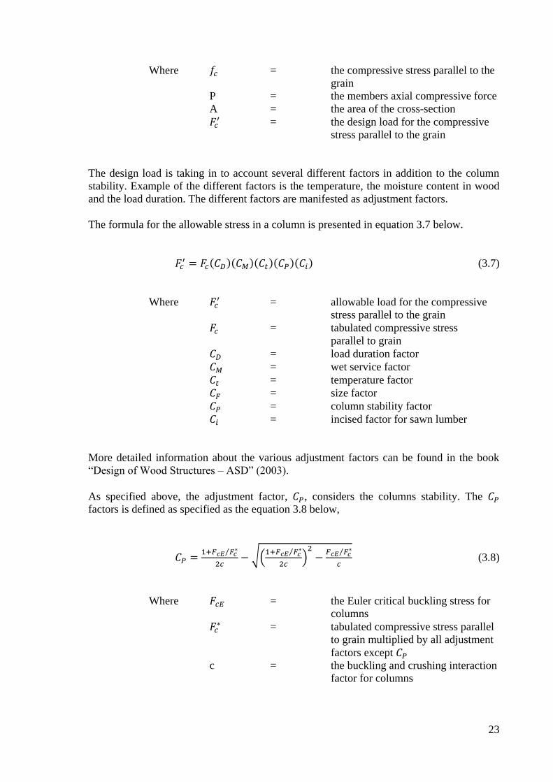
As specified above, the adjustment factor, , considers the columns stability. The
factors is defined as specified as the equation 3.8 below,
⁄
√(
⁄
)
⁄
(3.8)
Where = the Euler critical buckling stress for
columns
= tabulated compressive stress parallel
to grain multiplied by all adjustment
factors except
c = the buckling and crushing interaction
factor for columns
24
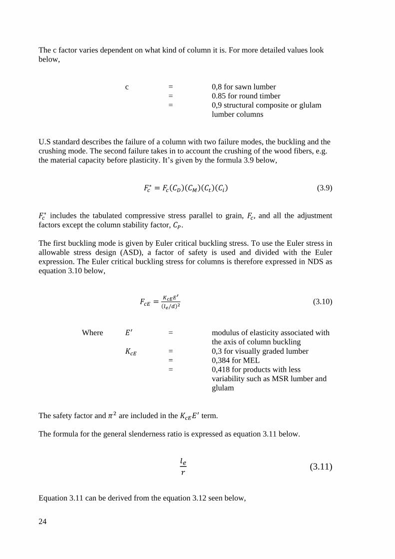
The c factor varies dependent on what kind of column it is. For more detailed values look
below,
c = 0,8 for sawn lumber
= 0.85 for round timber
= 0,9 structural composite or glulam
lumber columns
U.S standard describes the failure of a column with two failure modes, the buckling and the
crushing mode. The second failure takes in to account the crushing of the wood fibers, e.g.
the material capacity before plasticity. It’s given by the formula 3.9 below,
(3.9)
includes the tabulated compressive stress parallel to grain, and all the adjustment
factors except the column stability factor, .
The first buckling mode is given by Euler critical buckling stress. To use the Euler stress in
allowable stress design (ASD), a factor of safety is used and divided with the Euler
expression. The Euler critical buckling stress for columns is therefore expressed in NDS as
equation 3.10 below,
(3.10)
Where = modulus of elasticity associated with
the axis of column buckling
= 0,3 for visually graded lumber
= 0,384 for MEL
= 0,418 for products with less
variability such as MSR lumber and
glulam
The safety factor and are included in the term.
The formula for the general slenderness ratio is expressed as equation 3.11 below.
(3.11)
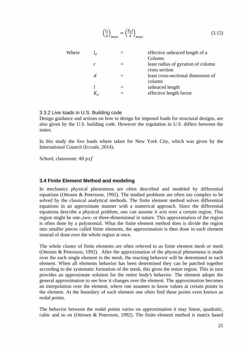
Equation 3.11 can be derived from the equation 3.12 seen below,
25
(
)
(
)
(3.12)
Where = effective unbraced length of a
Column
r = least radius of gyration of column
cross section
= least cross-sectional dimension of
column
= unbraced length
= effective length factor
3.3.2 Live loads in U.S. Building code Design guidance and actions on how to design for imposed loads for structural designs, are
also given by the U.S. building code. However the regulation in U.S. differs between the
states.
In this study the live loads where taken for New York City, which was given by the
International Council (Iccsafe, 2014).
School, classroom:
3.4 Finite Element Method and modeling
In mechanics physical phenomena are often described and modeled by differential
equations (Ottosen & Petersson, 1992). The studied problems are often too complex to be
solved by the classical analytical methods. The finite element method solves differential
equations in an approximate manner with a numerical approach. Since the differential
equations describe a physical problem, one can assume it acts over a certain region. This
region might be one-,two- or three-dimensional in nature. This approximation of the region
is often done by a polynomial. What the finite element method does is divide the region
into smaller pieces called finite elements, the approximation is then done in each element
instead of done over the whole region at once.
The whole cluster of finite elements are often referred to as finite element mesh or mesh
(Ottosen & Petersson, 1992). After the approximation of the physical phenomena is made
over the each single element in the mesh, the reacting behavior will be determined in each
element. When all elements behavior has been determined they can be patched together
according to the systematic formation of the mesh, this gives the entire region. This in turn
provides an approximate solution for the entire body's behavior. The element adopts the
general approximation to see how it changes over the element. The approximation becomes
an interpolation over the element, where one assumes to know values at certain points in
the element. At the boundary of each element one often find these points even known as
nodal points.
The behavior between the nodal points varies on approximation it may linear, quadratic,
cubic and so on (Ottosen & Petersson, 1992). The finite element method is matrix based
26
because it enables one to use thousands of unknown variables in a compact fashion. The
number of elements is crucial for the accuracy, more nodes means more accurate
approximation which in turn means that the solution will converge towards the actual case.
When one uses FE programs in practice the user still need to have the understanding of
underlying theories otherwise the result might be irrelevant.
3.4.1 Mathematical modeling This section is a review of the different approaches in mathematical modeling within FEM,
which is implemented to interpret the mechanical behavior.
3.4.1.1 First order theory In the first order theory, the applied load is directly proportional to the deformations and the
section forces, when a structure is of a linear elastic material (Runesson et al, 1992). This is
true as long as one assumes that the deformations are small and neglect able during
equilibrium equation. The original geometry of the structure is thus analyzed as a whole in
the first order theory. Each load can therefore be treated separately and later on be added to
the result since its linear, this is also referred as the superposition principle
3.4.1.2 Second order theory When some structures is subjected to utility loads significant deformations can occur, it’s
therefore important that one takes the size of the deformations into account alongside the
other geometry of the structure (Runesson et al, 1992).
In the second-order theory the structural deformations are still assumed to be small
(Runesson et al, 1992). But compared to the first-order theory the equilibrium equations in
the second-order theory consider the deformations. The superposition principle does
therefore not apply anymore and the relationship between the deformation and the load
generally isn’t linear, even for linear elastic material.
3.4.1.3 Third order theory By increasing realism further in the third order, deformations are no longer small and no
simplifications of geometry can be made, since the real geometry is the ground pillar to the
equilibrium equation (Runesson et al, 1992). Superposition principle is no longer possible,
neither is the possibility for simplifications for example, one can’t use the reduced
expression for curvature everything needs to be taken into account.
Comments:
To gain a better understanding of the linear elastic and inelastic behavior of the material the
FEM calculations will consider up to the second order.
27
4 Modeling
In this chapter methods and models of the different cases will be presented. The
calculations and modelling that are done in this report are based on the methods
prescribed in this chapter. The aim of this chapter is to describe the approach we take on
solving certain problems.
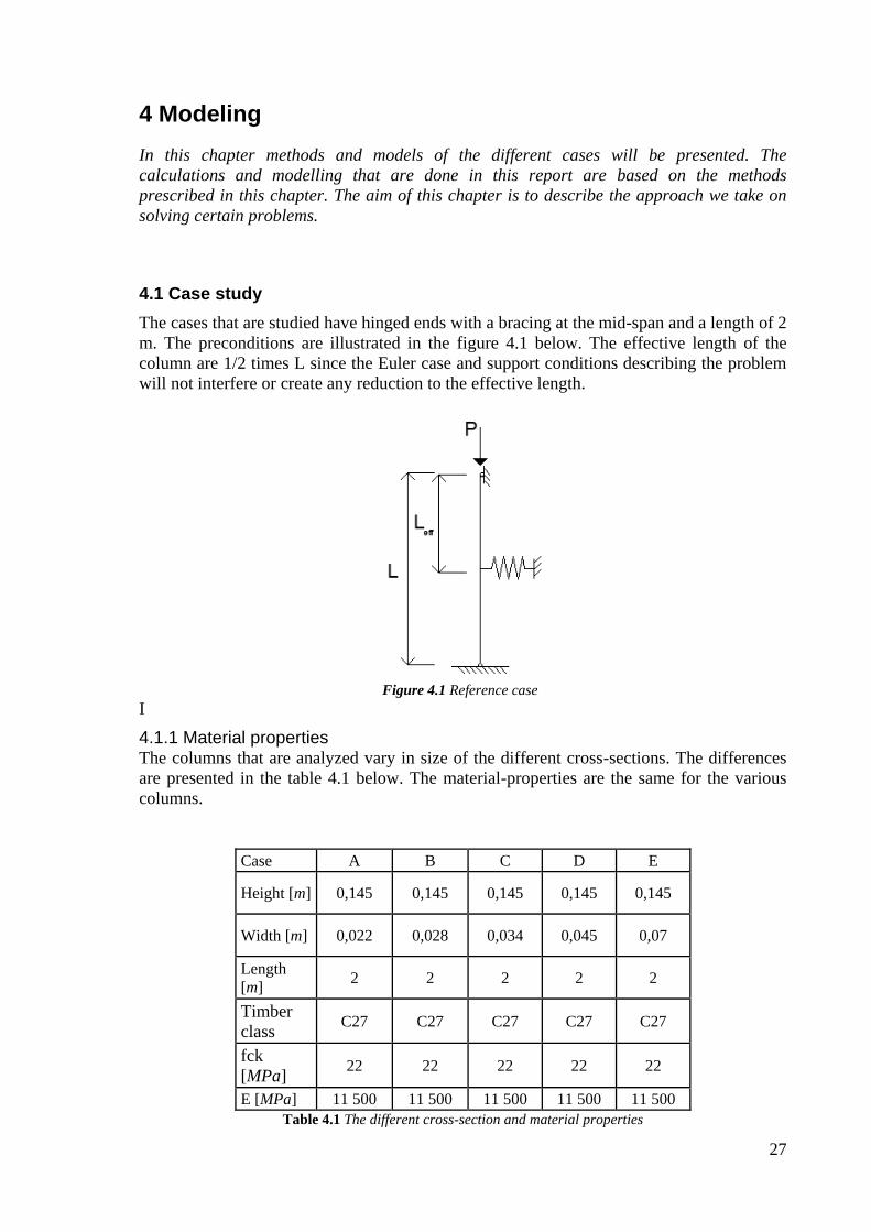
4.1 Case study
The cases that are studied have hinged ends with a bracing at the mid-span and a length of 2
m. The preconditions are illustrated in the figure 4.1 below. The effective length of the
column are 1/2 times L since the Euler case and support conditions describing the problem
will not interfere or create any reduction to the effective length.
Figure 4.1 Reference case
I
4.1.1 Material properties The columns that are analyzed vary in size of the different cross-sections. The differences
are presented in the table 4.1 below. The material-properties are the same for the various
columns.
Case A B C D E
Height [m] 0,145 0,145 0,145 0,145 0,145
Width [m] 0,022 0,028 0,034 0,045 0,07
Length
[m] 2 2 2 2 2
Timber
class C27 C27 C27 C27 C27
fck
[MPa] 22 22 22 22 22
E [MPa] 11 500 11 500 11 500 11 500 11 500
Table 4.1 The different cross-section and material properties

28
The cases studied are all targeted for column buckling at the weak side, this causes the
slenderness to be dependent by the width of the cross-section rather than the height in a
rectangular cross-section. The height is therefore kept constant for all cases. Other
geometrical information can be found in the following table 4.1 above.
4.2 Finite Element Method (FEM) model
This section introduces the method of how the FEM calculations are made. During FEM
calculations all cases are based on the reference case seen in 4.1.
Initial curvature is also pre-determined in all cases to 2 mm, L/500, unless it is otherwise
specified. The cross sections that are studied in second order analysis and have a
rectangular shape. The bracings are always placed on the weak direction since it's the side
that will give in first. Other presumptions during FEM are that each case is restricted in the
strong direction and rotations are presumed to be zero to prevent rigid body motion in those
cases it might occur.
4.2.1 Geometry The cases that are being studied are modeled in FEM into wire models. The reason behind
the use of the wire type is because of its accuracy and it gives a good approximation of the
case.
To create the model start of by draw a line of equivalent length to the case studied, then
apply the cross-section and material properties of the object. Since it’s a wire element the
user needs to specify an orientation of the line as well.
4.2.2 Load case When the geometry is done the load is applied in the form of a concentrated force on the
wire object.
During the linear perturbation buckling the force from the load is put to 1 so the resulting
eigenvalue will give you the load in Newton. The force is applied in the top of the wire
object.
In the second order the columns get a small initial curvature of L/500 so the simulation
reassembles a more realistic case. The loads in these cases are dependent on cross sections
and therefore different for all cases, to evaluate the load the linear perturbation buckling
calculation are made where the load is given in the shape of the eigenvalue.
4.2.3 Boundary conditions When it comes to limitations the program needs to know a reference in space where the
object is restricted. This is first done in assembly where the object is placed in a coordinate
system. Later one adds boundary conditions where the object gets given restriction
properties of how it should act in different directions in this space. Together it forces the
object in place when adding the applied load. The boundaries in these cases are given in
three points the two hinges at top and bottom together with the spring brace system in the
middle.
29
The boundary at the top is only restricted in x and z axis where the bottom is restricted in
the y axis as well as the others. The hinge boundary is placed in the middle of the top and
bottom part of the objects, this is done to best resemble a hinge.
When it comes to the spring on the other hand it is created by a specific type of boundary
condition called “spring to ground”, this causes one connection point to get a spring
restriction in one direction. The stiffness of the spring needs to be specified to know what
kind of resistance it causes to the system. During the second order the spring is considered
to be indispensable, and can therefore withstand forces acting on it. During other
calculations where the spring stiffness is evaluated it varies.
Since the cases are done in a three dimensions the nodes takes into account six different
values at each nodal point, displacements and rotations in x,y and z. Rotations are restricted
to prevent rigid body motion.
4.2.4 Mesh The key in a finite element method is the mesh, the matrix based appearance of the original
shape. Together with boundary conditions, load cases and the mesh FEM is capable to
calculate objects in a three dimensional space. The mesh size is dependent on the size of the
analyzed case, larger dimensions increases the mesh. More detailed mesh increases the
accuracy however and this cannot be over emphasized more detailed mesh takes more
computer power. In a perfect world one would have used infinitesimally small elements in a
mesh, but since the computer advancements of this day and age doesn’t allow it
simplifications needs to be made.
Everything is now in place to start calculating, when done the program gives the
displacements with the correlating force applied or other stresses dependent on what the
user specifies in the history output. At this point the data is converted over to excel to
restructure it and manage it further into tables and figures.
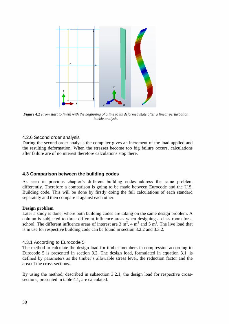
4.2.5 Linear perturbation buckle analysis The linear perturbation buckle analysis is preformed to gain the critical load for the studied
column case. This type of analysis will later be used as a reference case for how the initial
curvature shape will occur in the second order analysis.
30
Figure 4.2 From start to finish with the beginning of a line to its deformed state after a linear perturbation
buckle analysis.
4.2.6 Second order analysis During the second order analysis the computer gives an increment of the load applied and
the resulting deformation. When the stresses become too big failure occurs, calculations
after failure are of no interest therefore calculations stop there.
4.3 Comparison between the building codes
As seen in previous chapter’s different building codes address the same problem
differently. Therefore a comparison is going to be made between Eurocode and the U.S.
Building code. This will be done by firstly doing the full calculations of each standard
separately and then compare it against each other.
Design problem
Later a study is done, where both building codes are taking on the same design problem. A
column is subjected to three different influence areas when designing a class room for a
school. The different influence areas of interest are 3 m2, 4 m
2 and 5 m
2. The live load that
is in use for respective building code can be found in section 3.2.2 and 3.3.2.
4.3.1 According to Eurocode 5 The method to calculate the design load for timber members in compression according to
Eurocode 5 is presented in section 3.2. The design load, formulated in equation 3.1, is
defined by parameters as the timber’s allowable stress level, the reduction factor and the
area of the cross-sections.
By using the method, described in subsection 3.2.1, the design load for respective cross-
sections, presented in table 4.1, are calculated.
31
In the results the design load is used in order to compare Eurocode with the U.S. standard.
Kmod is given a value of 0.9 while calculating the design load.
4.3.2 According to the U.S. standard In section 3.3.1 the method to calculate the design load, according to the U.S. standard, for
timber members was presented. The design load is given in equation 3.6 where it is defined
that the subjected axial compressive stress in the member has to be lower than the capacity
of the column, which is defined by the columns allowable compressive stress.
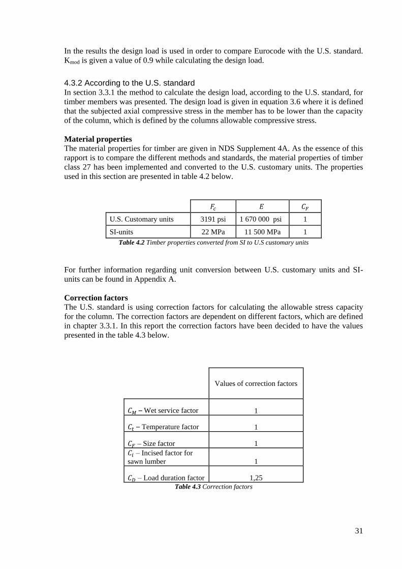
Material properties
The material properties for timber are given in NDS Supplement 4A. As the essence of this
rapport is to compare the different methods and standards, the material properties of timber
class 27 has been implemented and converted to the U.S. customary units. The properties
used in this section are presented in table 4.2 below.
U.S. Customary units 3191 psi 1 670 000 psi 1
SI-units 22 MPa 11 500 MPa 1
Table 4.2 Timber properties converted from SI to U.S customary units
For further information regarding unit conversion between U.S. customary units and SI-
units can be found in Appendix A.
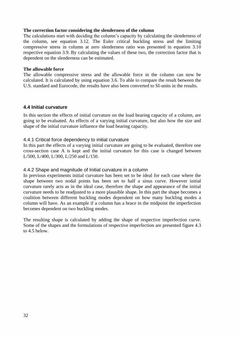
Correction factors
The U.S. standard is using correction factors for calculating the allowable stress capacity
for the column. The correction factors are dependent on different factors, which are defined
in chapter 3.3.1. In this report the correction factors have been decided to have the values
presented in the table 4.3 below.
Values of correction factors
– Wet service factor 1
– Temperature factor 1
– Size factor 1
– Incised factor for
sawn lumber 1
– Load duration factor 1,25
Table 4.3 Correction factors
32
The correction factor considering the slenderness of the column
The calculations start with deciding the column’s capacity by calculating the slenderness of
the column, see equation 3.12. The Euler critical buckling stress and the limiting
compressive stress in column at zero slenderness ratio was presented in equation 3.10
respective equation 3.9. By calculating the values of these two, the correction factor that is
dependent on the slenderness can be estimated.
The allowable force
The allowable compressive stress and the allowable force in the column can now be
calculated. It is calculated by using equation 3.6. To able to compare the result between the
U.S. standard and Eurocode, the results have also been converted to SI-units in the results.
4.4 Initial curvature
In this section the effects of initial curvature on the load bearing capacity of a column, are
going to be evaluated. As effects of a varying initial curvature, but also how the size and
shape of the initial curvature influence the load bearing capacity.
4.4.1 Critical force dependency to initial curvature In this part the effects of a varying initial curvature are going to be evaluated, therefore one
cross-section case A is kept and the initial curvature for this case is changed between
L/500, L/400, L/300, L/250 and L/150.
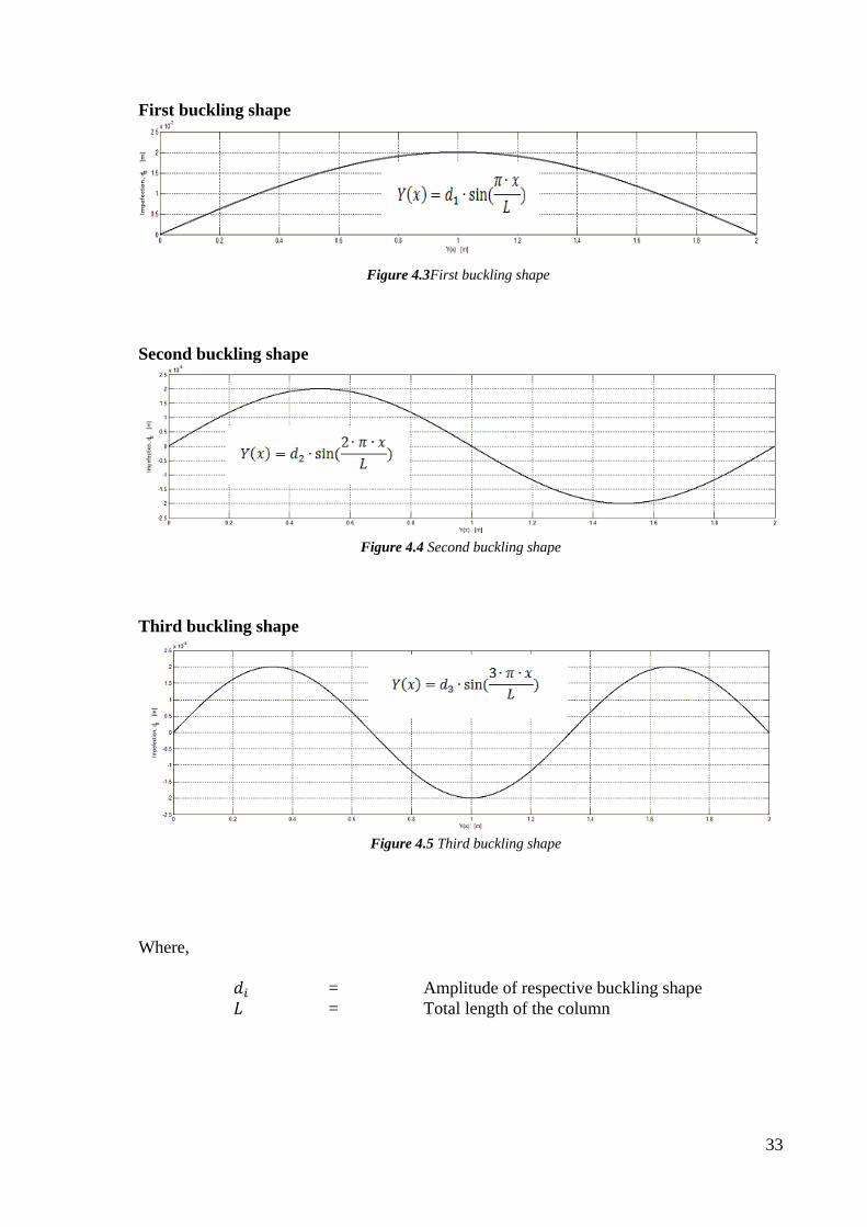
4.4.2 Shape and magnitude of Initial curvature in a column In previous experiments initial curvature has been set to be ideal for each case where the
shape between two nodal points has been set to half a sinus curve. However initial
curvature rarely acts as in the ideal case, therefore the shape and appearance of the initial
curvature needs to be readjusted to a more plausible shape. In this part the shape becomes a
coalition between different buckling modes dependent on how many buckling modes a
column will have. As an example if a column has a brace in the midpoint the imperfection
becomes dependent on two buckling modes.
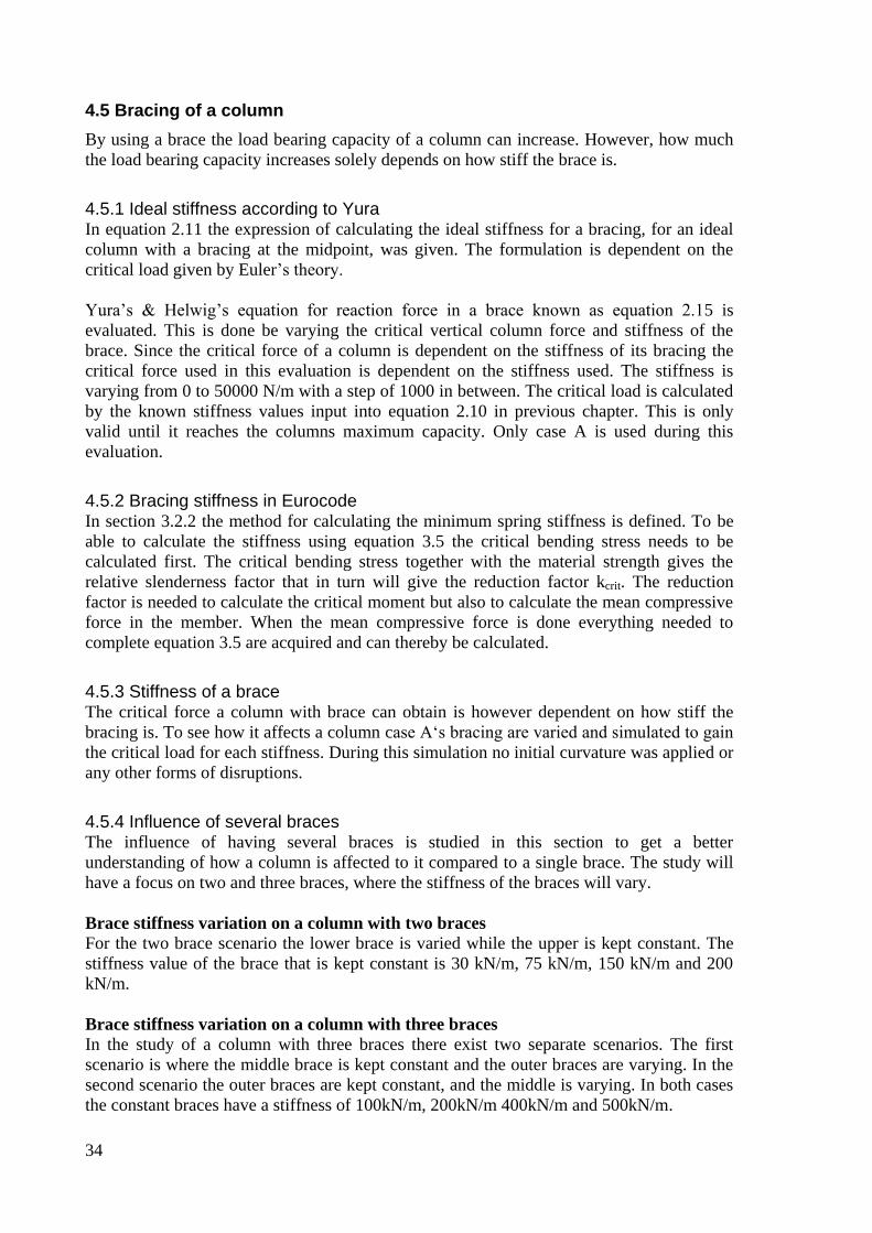
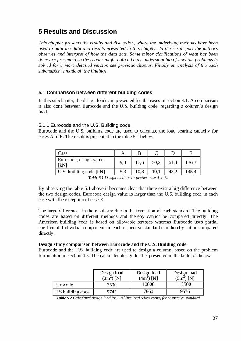
The resulting shape is calculated by adding the shape of respective imperfection curve.
Some of the shapes and the formulations of respective imperfection are presented figure 4.3
to 4.5 below.
33
First buckling shape
Figure 4.3First buckling shape
Second buckling shape
Figure 4.4 Second buckling shape
Third buckling shape
Figure 4.5 Third buckling shape
Where,
= Amplitude of respective buckling shape
= Total length of the column
34
4.5 Bracing of a column
By using a brace the load bearing capacity of a column can increase. However, how much
the load bearing capacity increases solely depends on how stiff the brace is.
4.5.1 Ideal stiffness according to Yura In equation 2.11 the expression of calculating the ideal stiffness for a bracing, for an ideal
column with a bracing at the midpoint, was given. The formulation is dependent on the
critical load given by Euler’s theory.
Yura’s & Helwig’s equation for reaction force in a brace known as equation 2.15 is
evaluated. This is done be varying the critical vertical column force and stiffness of the
brace. Since the critical force of a column is dependent on the stiffness of its bracing the
critical force used in this evaluation is dependent on the stiffness used. The stiffness is
varying from 0 to 50000 N/m with a step of 1000 in between. The critical load is calculated
by the known stiffness values input into equation 2.10 in previous chapter. This is only
valid until it reaches the columns maximum capacity. Only case A is used during this
evaluation.
4.5.2 Bracing stiffness in Eurocode In section 3.2.2 the method for calculating the minimum spring stiffness is defined. To be
able to calculate the stiffness using equation 3.5 the critical bending stress needs to be
calculated first. The critical bending stress together with the material strength gives the
relative slenderness factor that in turn will give the reduction factor kcrit. The reduction
factor is needed to calculate the critical moment but also to calculate the mean compressive
force in the member. When the mean compressive force is done everything needed to
complete equation 3.5 are acquired and can thereby be calculated.
4.5.3 Stiffness of a brace The critical force a column with brace can obtain is however dependent on how stiff the
bracing is. To see how it affects a column case A‘s bracing are varied and simulated to gain
the critical load for each stiffness. During this simulation no initial curvature was applied or
any other forms of disruptions.
4.5.4 Influence of several braces The influence of having several braces is studied in this section to get a better
understanding of how a column is affected to it compared to a single brace. The study will
have a focus on two and three braces, where the stiffness of the braces will vary.
Brace stiffness variation on a column with two braces
For the two brace scenario the lower brace is varied while the upper is kept constant. The
stiffness value of the brace that is kept constant is 30 kN/m, 75 kN/m, 150 kN/m and 200
kN/m.
Brace stiffness variation on a column with three braces
In the study of a column with three braces there exist two separate scenarios. The first
scenario is where the middle brace is kept constant and the outer braces are varying. In the
second scenario the outer braces are kept constant, and the middle is varying. In both cases
the constant braces have a stiffness of 100kN/m, 200kN/m 400kN/m and 500kN/m.

35
4.5.5 Brace force study To evaluate the study of bracings further, a study of the reaction force in the brace is done.
This is done to verify Yura’s equation of a brace force seen in equation 2.15. This is
compared in FEM by varying the vertical column force and the stiffness of the brace. This
is done be varying the critical vertical column force and stiffness of the brace. Since the
critical force of a column is dependent on the stiffness of its bracing, the force applied is
always set so the critical force for each stiffness case used during this evaluation.
The critical load is calculated by linear buckling analysis which uses the stiffness
prescribed. This is only valid until it reaches the columns maximum capacity. Only case A
is used during this evaluation with an initial curvature of d0 = 2mm.
4.5.6 Influence of initial curvature Lastly the initial curvature is changed to see its effect of how the reaction force in a brace is
in correlation to the initial curvature, and how it behaves for a known bracing stiffness. The
known brace stiffness that is evaluated is 50000 N/m and 40000 N/m. The load that acts on
the column is restricted by the columns load bearing capacity. The results is therefore
restricted to p/pcr = 1 throughout the evaluation.

36
37
5 Results and Discussion
This chapter presents the results and discussion, where the underlying methods have been
used to gain the data and results presented in this chapter. In the result part the authors
observes and interpret of how the data acts. Some minor clarifications of what has been
done are presented so the reader might gain a better understanding of how the problems is
solved for a more detailed version see previous chapter. Finally an analysis of the each
subchapter is made of the findings.
5.1 Comparison between different building codes
In this subchapter, the design loads are presented for the cases in section 4.1. A comparison
is also done between Eurocode and the U.S. building code, regarding a column’s design
load.
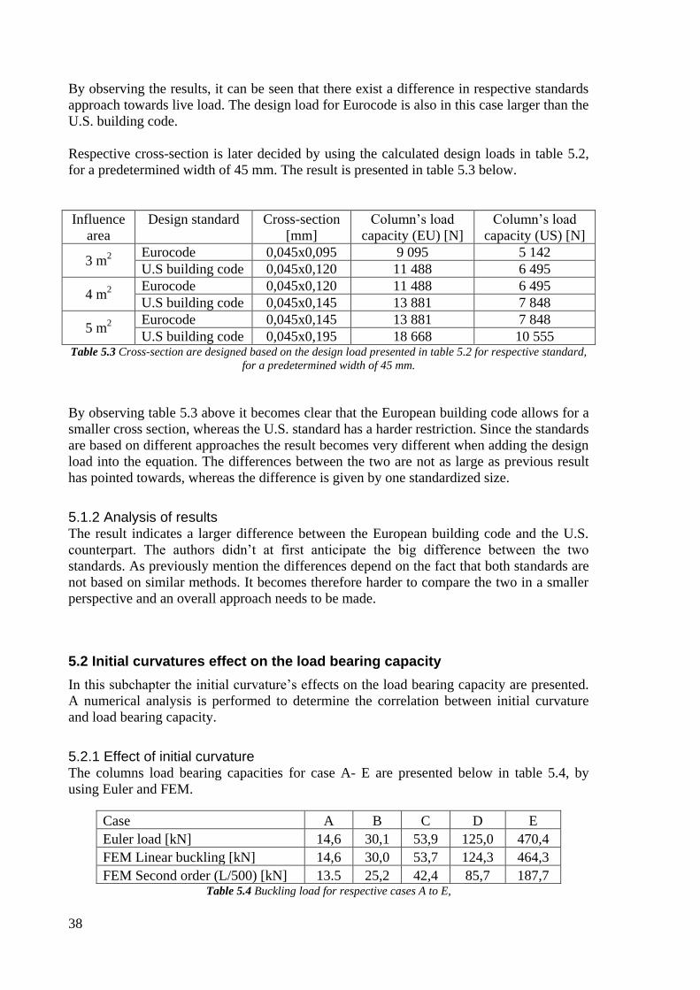
5.1.1 Eurocode and the U.S. Building code Eurocode and the U.S. building code are used to calculate the load bearing capacity for
cases A to E. The result is presented in the table 5.1 below.
Case A B C D E
Eurocode, design value
[kN] 9,3 17,6 30,2 61,4 136,3
U.S. building code [kN] 5,3 10,8 19,1 43,2 145,4
Table 5.1 Design load for respective case A to E.
By observing the table 5.1 above it becomes clear that there exist a big difference between
the two design codes. Eurocode design value is larger than the U.S. building code in each
case with the exception of case E.
The large differences in the result are due to the formation of each standard. The building
codes are based on different methods and thereby cannot be compared directly. The
American building code is based on allowable stresses whereas Eurocode uses partial
coefficient. Individual components in each respective standard can thereby not be compared
directly.
Design study comparison between Eurocode and the U.S. Building code
Eurocode and the U.S. building code are used to design a column, based on the problem
formulation in section 4.3. The calculated design load is presented in the table 5.2 below.
Design load
(3m2) [N]
Design load
(4m2) [N]
Design load
(5m2) [N]
Eurocode 7500 10000 12500
U.S building code 5745 7660 9576
Table 5.2 Calculated design load for 3 m2 live load (class room) for respective standard
38
By observing the results, it can be seen that there exist a difference in respective standards
approach towards live load. The design load for Eurocode is also in this case larger than the
U.S. building code.
Respective cross-section is later decided by using the calculated design loads in table 5.2,
for a predetermined width of 45 mm. The result is presented in table 5.3 below.
Influence
area
Design standard Cross-section
[mm]
Column’s load
capacity (EU) [N]
Column’s load
capacity (US) [N]
3 m2
Eurocode 0,045x0,095 9 095 5 142
U.S building code 0,045x0,120 11 488 6 495
4 m2
Eurocode 0,045x0,120 11 488 6 495
U.S building code 0,045x0,145 13 881 7 848
5 m2
Eurocode 0,045x0,145 13 881 7 848
U.S building code 0,045x0,195 18 668 10 555 Table 5.3 Cross-section are designed based on the design load presented in table 5.2 for respective standard,
for a predetermined width of 45 mm.
By observing table 5.3 above it becomes clear that the European building code allows for a
smaller cross section, whereas the U.S. standard has a harder restriction. Since the standards
are based on different approaches the result becomes very different when adding the design
load into the equation. The differences between the two are not as large as previous result
has pointed towards, whereas the difference is given by one standardized size.
5.1.2 Analysis of results The result indicates a larger difference between the European building code and the U.S.
counterpart. The authors didn’t at first anticipate the big difference between the two
standards. As previously mention the differences depend on the fact that both standards are
not based on similar methods. It becomes therefore harder to compare the two in a smaller
perspective and an overall approach needs to be made.
5.2 Initial curvatures effect on the load bearing capacity
In this subchapter the initial curvature’s effects on the load bearing capacity are presented.
A numerical analysis is performed to determine the correlation between initial curvature
and load bearing capacity.
5.2.1 Effect of initial curvature The columns load bearing capacities for case A- E are presented below in table 5.4, by
using Euler and FEM.
Case A B C D E
Euler load [kN] 14,6 30,1 53,9 125,0 470,4
FEM Linear buckling [kN] 14,6 30,0 53,7 124,3 464,3
FEM Second order (L/500) [kN] 13.5 25,2 42,4 85,7 187,7 Table 5.4 Buckling load for respective cases A to E,

39
By observing the results in table 5.4, one can see that the Euler load and the FEM linear
analysis are similar. They should theoretically be the same since they both use the same
method. The reason behind why Euler’s load and FEM linear analysis differs could be
because of Euler’s load is meant for slender columns.
The force- and deformation correlation for FEM secondary analysis is presented in the
figure 5.1 below.
Figure 5.1 Force - Deformation diagram for case A to E, with an initial curvature of d0 = 2
mm
Comparing the Euler buckling load and the buckling load based on FEM second order
analysis in table 5.4, a large difference becomes present. Second order indicates a smaller
capacity since it takes imperfections and smaller deformations into account, which can be
seen in table 5.4. The column’s load bearing capacity is therefore smaller than an ideal
column. Figure 5.1 illustrates the nonlinear effects of the deformation in the second order
analysis.
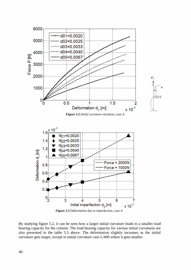
5.2.2 Critical force dependency due to initial curvature Table 5.5 and figure 5.2 below presents the resulting load bearing capacity and deformation
of a column due to a varying initial curvature. The different initial curvature cases are set
from the smallest L/500 (d01) to the largest L/150 (d05), and are based on Case A. To
evaluate each imperfection with resulting deformation a bit closer figure 5.3 below will
display how it behave during two known forces.
Initial curvature case L/500 L/400 L/300 L/250 L/150
Initail curvature d0 [mm] 2 2,5 3,3 4 6,7
Force [kN] 5,32 4,60 3,87 3,38 2,29
Deformation d1 [mm] 1,86 1,78 1,80 1,77 1,75 Table 5.5 Initial curvature cases
40
Figure 5.2 Initial curvature variation, case A
Figure 5.3 Deformation due to imperfection, case A
By studying figure 5.2, it can be seen how a larger initial curvature leads to a smaller load
bearing capacity for the column. The load bearing capacity for various initial curvatures are
also presented in the table 5.5 above. The deformation slightly increases as the initial
curvature gets larger, except in initial curvature case L/400 where it gets smaller.
41
In figure 5.3 one can see that larger initial curvature leads to an increased rate of
deformation. The deformation rate is with other words dependent on the initial curvature of
the column.
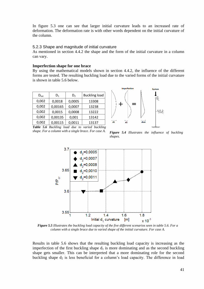
5.2.3 Shape and magnitude of initial curvature As mentioned in section 4.4.2 the shape and the form of the initial curvature in a column
can vary.
Imperfection shape for one brace
By using the mathematical models shown in section 4.4.2, the influence of the different
forms are tested. The resulting buckling load due to the varied forms of the initial curvature
is shown in table 5.6 below.
Dtot D1 D2 Buckling load
0,002 0,0018 0,0005 13308
0,002 0,00165 0,0007 13238
0,002 0,0015 0,0008 13222
0,002 0,00135 0,001 13142
0,002 0,00115 0,0011 13137 Table 5.6 Buckling load due to varied buckling
shape. For a column with a single brace. For case A.
Figure 5.4 Illustrates the influence of buckling
shapes.
Figure 5.5 Illustrates the buckling load capacity of the five different scenarios seen in table 5.6. For a
column with a single brace due to varied shape of the initial curvature. For case A.
Results in table 5.6 shows that the resulting buckling load capacity is increasing as the
imperfection of the first buckling shape d1 is more dominating and as the second buckling
shape gets smaller. This can be interpreted that a more dominating role for the second
buckling shape d2 is less beneficial for a column’s load capacity. The difference in load
42
buckling capacity between a more dominating d1 and d2 is though very small in this
example.
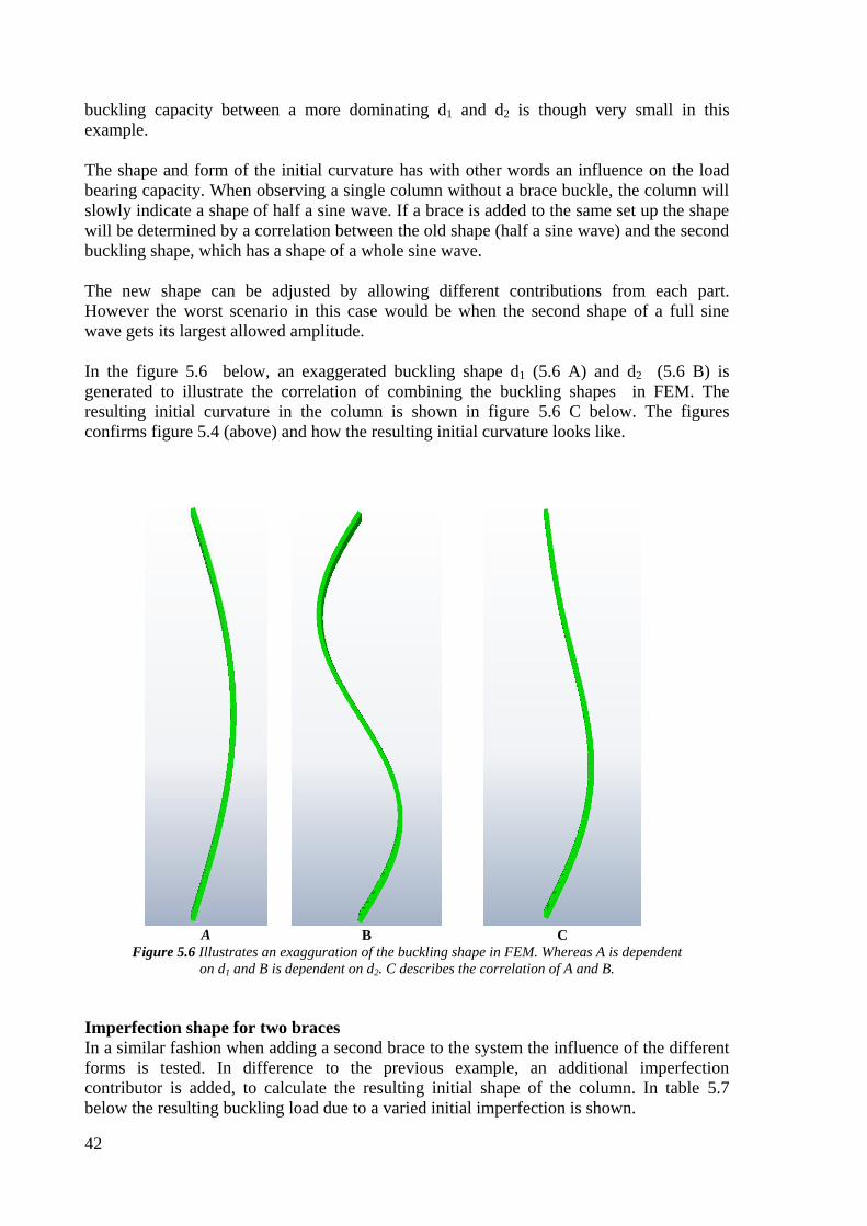
The shape and form of the initial curvature has with other words an influence on the load
bearing capacity. When observing a single column without a brace buckle, the column will
slowly indicate a shape of half a sine wave. If a brace is added to the same set up the shape
will be determined by a correlation between the old shape (half a sine wave) and the second
buckling shape, which has a shape of a whole sine wave.
The new shape can be adjusted by allowing different contributions from each part.
However the worst scenario in this case would be when the second shape of a full sine
wave gets its largest allowed amplitude.
In the figure 5.6 below, an exaggerated buckling shape d1 (5.6 A) and d2 (5.6 B) is
generated to illustrate the correlation of combining the buckling shapes in FEM. The
resulting initial curvature in the column is shown in figure 5.6 C below. The figures
confirms figure 5.4 (above) and how the resulting initial curvature looks like.
A
B
C
Figure 5.6 Illustrates an exagguration of the buckling shape in FEM. Whereas A is dependent
on d1 and B is dependent on d2. C describes the correlation of A and B.
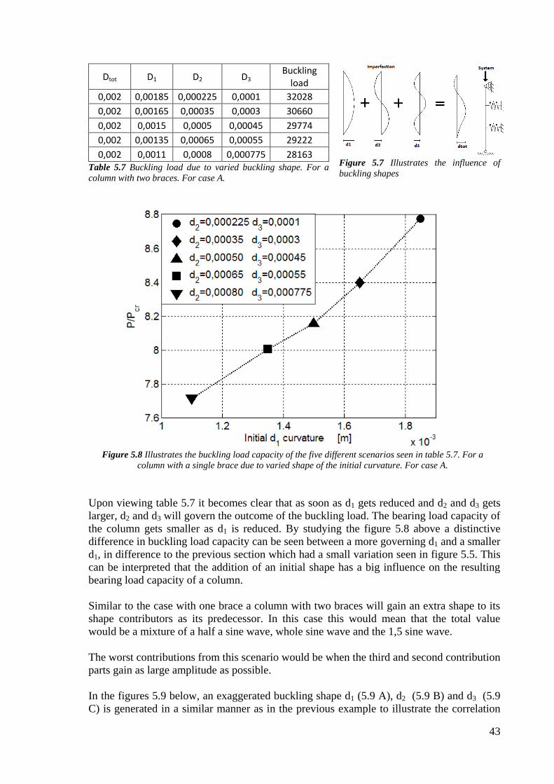
Imperfection shape for two braces
In a similar fashion when adding a second brace to the system the influence of the different
forms is tested. In difference to the previous example, an additional imperfection
contributor is added, to calculate the resulting initial shape of the column. In table 5.7
below the resulting buckling load due to a varied initial imperfection is shown.
43
Dtot D1 D2 D3 Buckling
load
0,002 0,00185 0,000225 0,0001 32028
0,002 0,00165 0,00035 0,0003 30660
0,002 0,0015 0,0005 0,00045 29774
0,002 0,00135 0,00065 0,00055 29222
0,002 0,0011 0,0008 0,000775 28163 Table 5.7 Buckling load due to varied buckling shape. For a
column with two braces. For case A.
Figure 5.7 Illustrates the influence of
buckling shapes
Figure 5.8 Illustrates the buckling load capacity of the five different scenarios seen in table 5.7. For a
column with a single brace due to varied shape of the initial curvature. For case A.
Upon viewing table 5.7 it becomes clear that as soon as d1 gets reduced and d2 and d3 gets
larger, d2 and d3 will govern the outcome of the buckling load. The bearing load capacity of
the column gets smaller as d1 is reduced. By studying the figure 5.8 above a distinctive
difference in buckling load capacity can be seen between a more governing d1 and a smaller
d1, in difference to the previous section which had a small variation seen in figure 5.5. This
can be interpreted that the addition of an initial shape has a big influence on the resulting
bearing load capacity of a column.
Similar to the case with one brace a column with two braces will gain an extra shape to its
shape contributors as its predecessor. In this case this would mean that the total value
would be a mixture of a half a sine wave, whole sine wave and the 1,5 sine wave.
The worst contributions from this scenario would be when the third and second contribution
parts gain as large amplitude as possible.
In the figures 5.9 below, an exaggerated buckling shape d1 (5.9 A), d2 (5.9 B) and d3 (5.9
C) is generated in a similar manner as in the previous example to illustrate the correlation
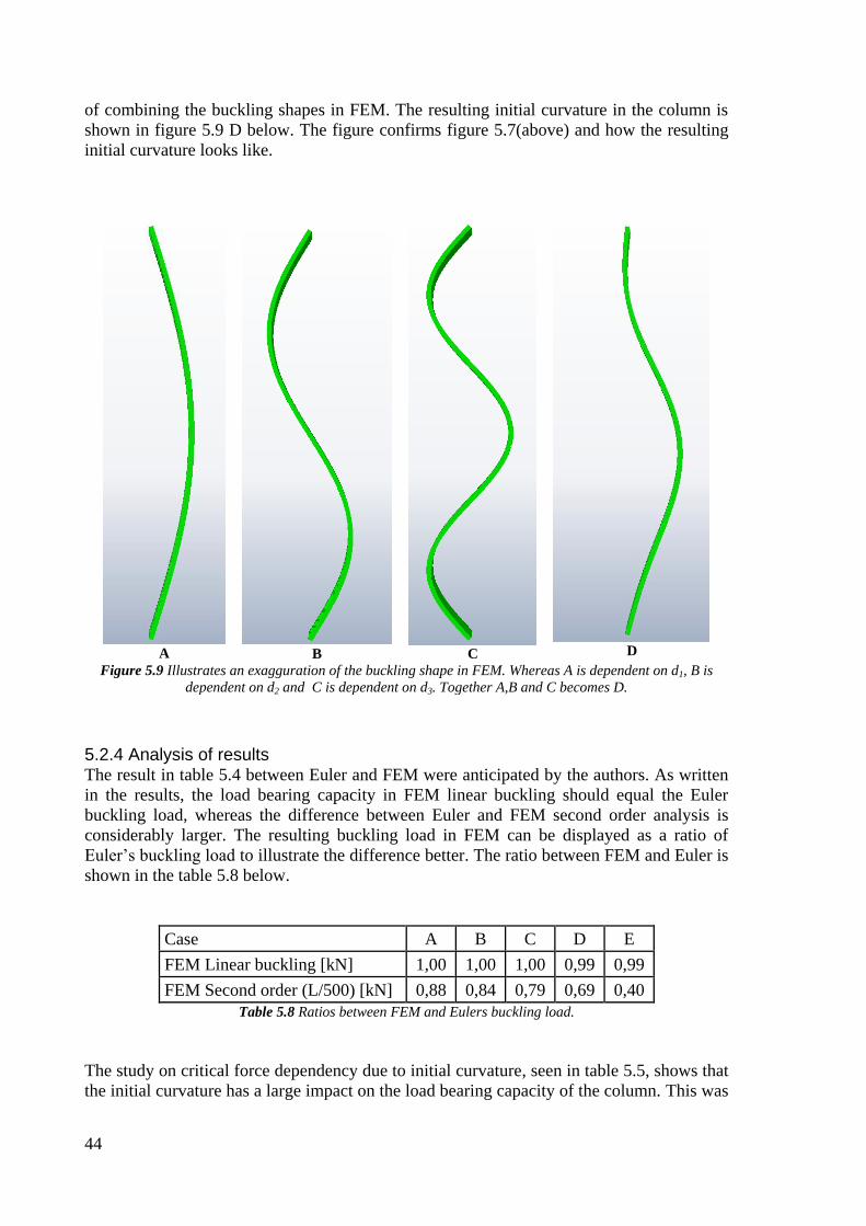
44
of combining the buckling shapes in FEM. The resulting initial curvature in the column is
shown in figure 5.9 D below. The figure confirms figure 5.7(above) and how the resulting
initial curvature looks like.
A
B
C
D
Figure 5.9 Illustrates an exagguration of the buckling shape in FEM. Whereas A is dependent on d1, B is
dependent on d2 and C is dependent on d3. Together A,B and C becomes D.
5.2.4 Analysis of results The result in table 5.4 between Euler and FEM were anticipated by the authors. As written
in the results, the load bearing capacity in FEM linear buckling should equal the Euler
buckling load, whereas the difference between Euler and FEM second order analysis is
considerably larger. The resulting buckling load in FEM can be displayed as a ratio of
Euler’s buckling load to illustrate the difference better. The ratio between FEM and Euler is
shown in the table 5.8 below.
Case A B C D E
FEM Linear buckling [kN] 1,00 1,00 1,00 0,99 0,99
FEM Second order (L/500) [kN] 0,88 0,84 0,79 0,69 0,40
Table 5.8 Ratios between FEM and Eulers buckling load.
The study on critical force dependency due to initial curvature, seen in table 5.5, shows that
the initial curvature has a large impact on the load bearing capacity of the column. This was
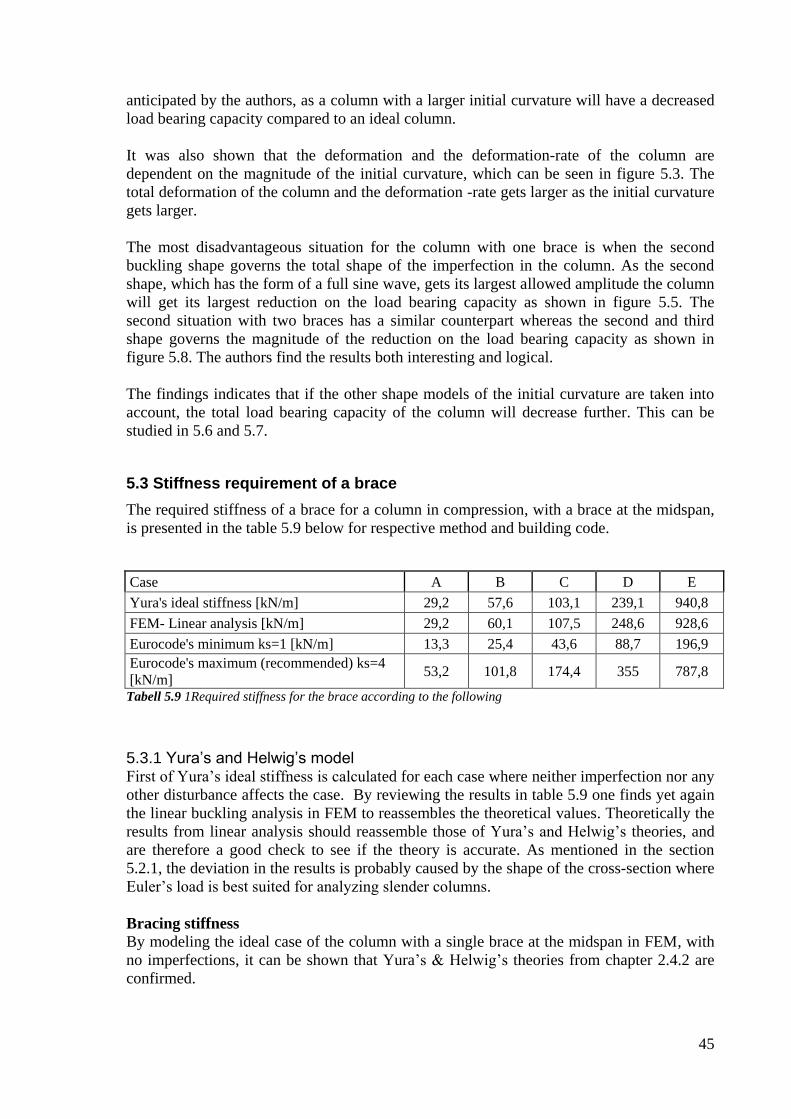
45
anticipated by the authors, as a column with a larger initial curvature will have a decreased
load bearing capacity compared to an ideal column.
It was also shown that the deformation and the deformation-rate of the column are
dependent on the magnitude of the initial curvature, which can be seen in figure 5.3. The
total deformation of the column and the deformation -rate gets larger as the initial curvature
gets larger.
The most disadvantageous situation for the column with one brace is when the second
buckling shape governs the total shape of the imperfection in the column. As the second
shape, which has the form of a full sine wave, gets its largest allowed amplitude the column
will get its largest reduction on the load bearing capacity as shown in figure 5.5. The
second situation with two braces has a similar counterpart whereas the second and third
shape governs the magnitude of the reduction on the load bearing capacity as shown in
figure 5.8. The authors find the results both interesting and logical.
The findings indicates that if the other shape models of the initial curvature are taken into
account, the total load bearing capacity of the column will decrease further. This can be
studied in 5.6 and 5.7.
5.3 Stiffness requirement of a brace
The required stiffness of a brace for a column in compression, with a brace at the midspan,
is presented in the table 5.9 below for respective method and building code.
Case A B C D E
Yura's ideal stiffness [kN/m] 29,2 57,6 103,1 239,1 940,8
FEM- Linear analysis [kN/m] 29,2 60,1 107,5 248,6 928,6
Eurocode's minimum ks=1 [kN/m] 13,3 25,4 43,6 88,7 196,9
Eurocode's maximum (recommended) ks=4
[kN/m] 53,2 101,8 174,4 355 787,8
Tabell 5.9 1Required stiffness for the brace according to the following
5.3.1 Yura’s and Helwig’s model First of Yura’s ideal stiffness is calculated for each case where neither imperfection nor any
other disturbance affects the case. By reviewing the results in table 5.9 one finds yet again
the linear buckling analysis in FEM to reassembles the theoretical values. Theoretically the
results from linear analysis should reassemble those of Yura’s and Helwig’s theories, and
are therefore a good check to see if the theory is accurate. As mentioned in the section
5.2.1, the deviation in the results is probably caused by the shape of the cross-section where
Euler’s load is best suited for analyzing slender columns.
Bracing stiffness
By modeling the ideal case of the column with a single brace at the midspan in FEM, with
no imperfections, it can be shown that Yura’s & Helwig’s theories from chapter 2.4.2 are
confirmed.
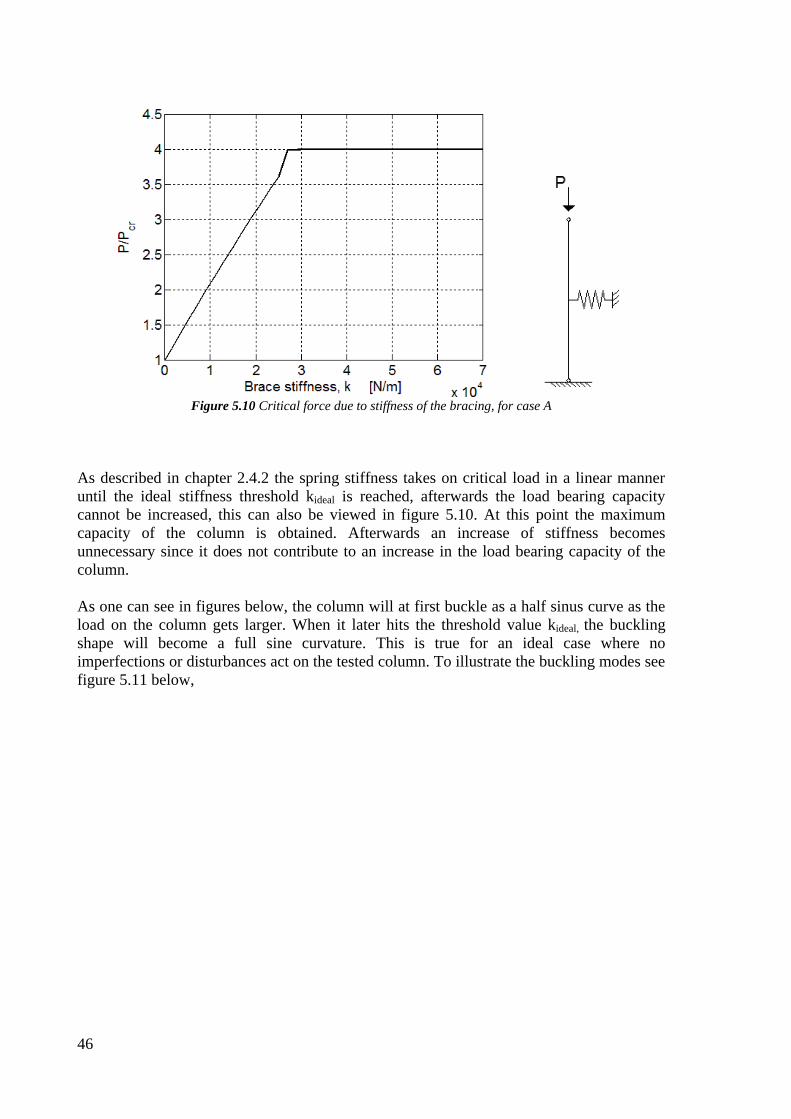
46
Figure 5.10 Critical force due to stiffness of the bracing, for case A
As described in chapter 2.4.2 the spring stiffness takes on critical load in a linear manner
until the ideal stiffness threshold kideal is reached, afterwards the load bearing capacity
cannot be increased, this can also be viewed in figure 5.10. At this point the maximum
capacity of the column is obtained. Afterwards an increase of stiffness becomes
unnecessary since it does not contribute to an increase in the load bearing capacity of the
column.
As one can see in figures below, the column will at first buckle as a half sinus curve as the
load on the column gets larger. When it later hits the threshold value kideal, the buckling
shape will become a full sine curvature. This is true for an ideal case where no
imperfections or disturbances act on the tested column. To illustrate the buckling modes see
figure 5.11 below,
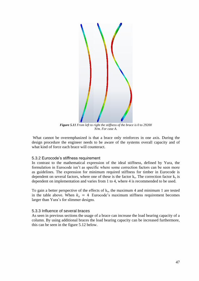
47
Figure 5.11 From left to right the stiffness of the brace is 0 to 29200
N/m. For case A.
What cannot be overemphasized is that a brace only reinforces in one axis. During the
design procedure the engineer needs to be aware of the systems overall capacity and of
what kind of force each brace will counteract.
5.3.2 Eurocode’s stiffness requirement In contrast to the mathematical expression of the ideal stiffness, defined by Yura, the
formulation in Eurocode isn’t as specific where some correction factors can be seen more
as guidelines. The expression for minimum required stiffness for timber in Eurocode is
dependent on several factors, where one of these is the factor ks. The correction factor ks is
dependent on implementation and varies from 1 to 4, where 4 is recommended to be used.
To gain a better perspective of the effects of ks, the maximum 4 and minimum 1 are tested
in the table above. When Eurocode’s maximum stiffness requirement becomes
larger than Yura’s for slimmer designs.
5.3.3 Influence of several braces As seen in previous sections the usage of a brace can increase the load bearing capacity of a
column. By using additional braces the load bearing capacity can be increased furthermore,
this can be seen in the figure 5.12 below.
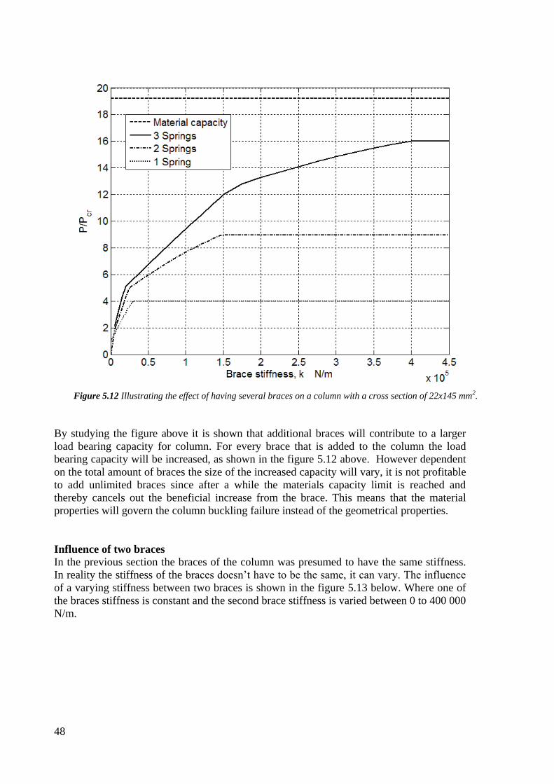
48
Figure 5.12 Illustrating the effect of having several braces on a column with a cross section of 22x145 mm2.
By studying the figure above it is shown that additional braces will contribute to a larger
load bearing capacity for column. For every brace that is added to the column the load
bearing capacity will be increased, as shown in the figure 5.12 above. However dependent
on the total amount of braces the size of the increased capacity will vary, it is not profitable
to add unlimited braces since after a while the materials capacity limit is reached and
thereby cancels out the beneficial increase from the brace. This means that the material
properties will govern the column buckling failure instead of the geometrical properties.
Influence of two braces
In the previous section the braces of the column was presumed to have the same stiffness.
In reality the stiffness of the braces doesn’t have to be the same, it can vary. The influence
of a varying stiffness between two braces is shown in the figure 5.13 below. Where one of
the braces stiffness is constant and the second brace stiffness is varied between 0 to 400 000
N/m.
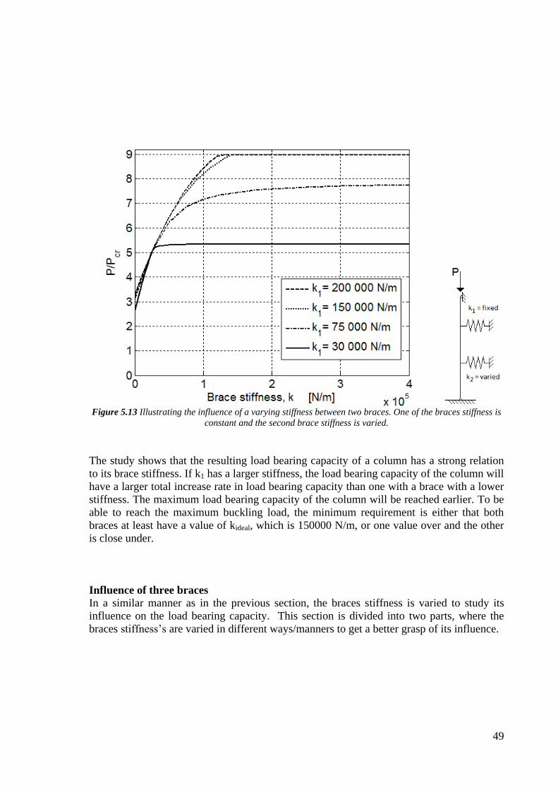
49
Figure 5.13 Illustrating the influence of a varying stiffness between two braces. One of the braces stiffness is
constant and the second brace stiffness is varied.
The study shows that the resulting load bearing capacity of a column has a strong relation
to its brace stiffness. If k1 has a larger stiffness, the load bearing capacity of the column will
have a larger total increase rate in load bearing capacity than one with a brace with a lower
stiffness. The maximum load bearing capacity of the column will be reached earlier. To be
able to reach the maximum buckling load, the minimum requirement is either that both
braces at least have a value of kideal, which is 150000 N/m, or one value over and the other
is close under.
Influence of three braces
In a similar manner as in the previous section, the braces stiffness is varied to study its
influence on the load bearing capacity. This section is divided into two parts, where the
braces stiffness’s are varied in different ways/manners to get a better grasp of its influence.
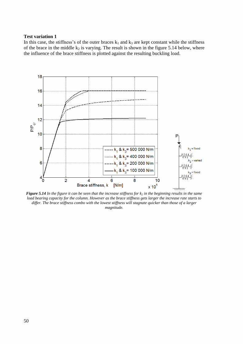
50
Test variation 1
In this case, the stiffness’s of the outer braces k1 and k3 are kept constant while the stiffness
of the brace in the middle k2 is varying. The result is shown in the figure 5.14 below, where
the influence of the brace stiffness is plotted against the resulting buckling load.
Figure 5.14 In the figure it can be seen that the increase stiffness for k2 in the beginning results in the same
load bearing capacity for the column. However as the brace stiffness gets larger the increase rate starts to
differ. The brace stiffness combo with the lowest stiffness will stagnate quicker than those of a larger
magnitude.
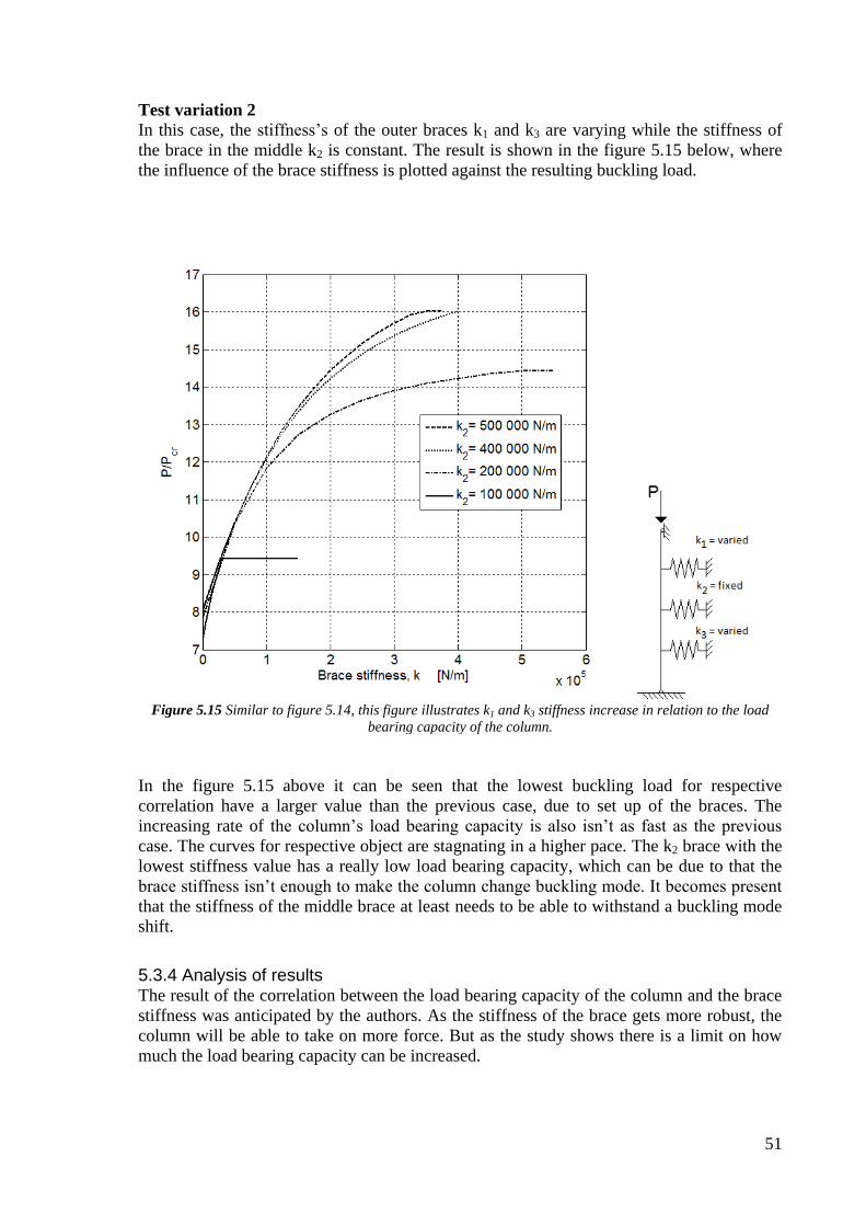
51
Test variation 2
In this case, the stiffness’s of the outer braces k1 and k3 are varying while the stiffness of
the brace in the middle k2 is constant. The result is shown in the figure 5.15 below, where
the influence of the brace stiffness is plotted against the resulting buckling load.
Figure 5.15 Similar to figure 5.14, this figure illustrates k1 and k3 stiffness increase in relation to the load
bearing capacity of the column.
In the figure 5.15 above it can be seen that the lowest buckling load for respective
correlation have a larger value than the previous case, due to set up of the braces. The
increasing rate of the column’s load bearing capacity is also isn’t as fast as the previous
case. The curves for respective object are stagnating in a higher pace. The k2 brace with the
lowest stiffness value has a really low load bearing capacity, which can be due to that the
brace stiffness isn’t enough to make the column change buckling mode. It becomes present
that the stiffness of the middle brace at least needs to be able to withstand a buckling mode
shift.
5.3.4 Analysis of results The result of the correlation between the load bearing capacity of the column and the brace
stiffness was anticipated by the authors. As the stiffness of the brace gets more robust, the
column will be able to take on more force. But as the study shows there is a limit on how
much the load bearing capacity can be increased.
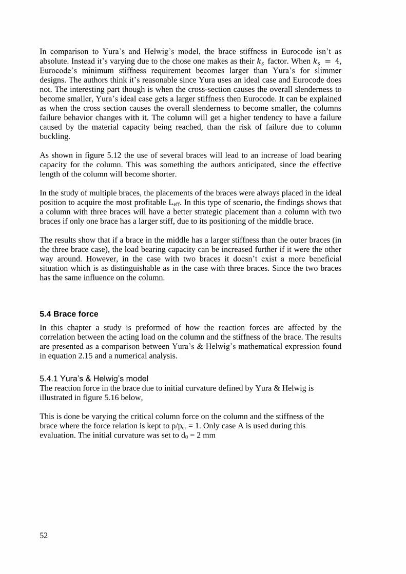
52
In comparison to Yura’s and Helwig’s model, the brace stiffness in Eurocode isn’t as
absolute. Instead it’s varying due to the chose one makes as their factor. When ,
Eurocode’s minimum stiffness requirement becomes larger than Yura’s for slimmer
designs. The authors think it’s reasonable since Yura uses an ideal case and Eurocode does
not. The interesting part though is when the cross-section causes the overall slenderness to
become smaller, Yura’s ideal case gets a larger stiffness then Eurocode. It can be explained
as when the cross section causes the overall slenderness to become smaller, the columns
failure behavior changes with it. The column will get a higher tendency to have a failure
caused by the material capacity being reached, than the risk of failure due to column
buckling.
As shown in figure 5.12 the use of several braces will lead to an increase of load bearing
capacity for the column. This was something the authors anticipated, since the effective
length of the column will become shorter.
In the study of multiple braces, the placements of the braces were always placed in the ideal
position to acquire the most profitable Leff. In this type of scenario, the findings shows that
a column with three braces will have a better strategic placement than a column with two
braces if only one brace has a larger stiff, due to its positioning of the middle brace.
The results show that if a brace in the middle has a larger stiffness than the outer braces (in
the three brace case), the load bearing capacity can be increased further if it were the other
way around. However, in the case with two braces it doesn’t exist a more beneficial
situation which is as distinguishable as in the case with three braces. Since the two braces
has the same influence on the column.
5.4 Brace force
In this chapter a study is preformed of how the reaction forces are affected by the
correlation between the acting load on the column and the stiffness of the brace. The results
are presented as a comparison between Yura’s & Helwig’s mathematical expression found
in equation 2.15 and a numerical analysis.
5.4.1 Yura’s & Helwig’s model The reaction force in the brace due to initial curvature defined by Yura & Helwig is
illustrated in figure 5.16 below,
This is done be varying the critical column force on the column and the stiffness of the
brace where the force relation is kept to p/pcr = 1. Only case A is used during this
evaluation. The initial curvature was set to d0 = 2 mm
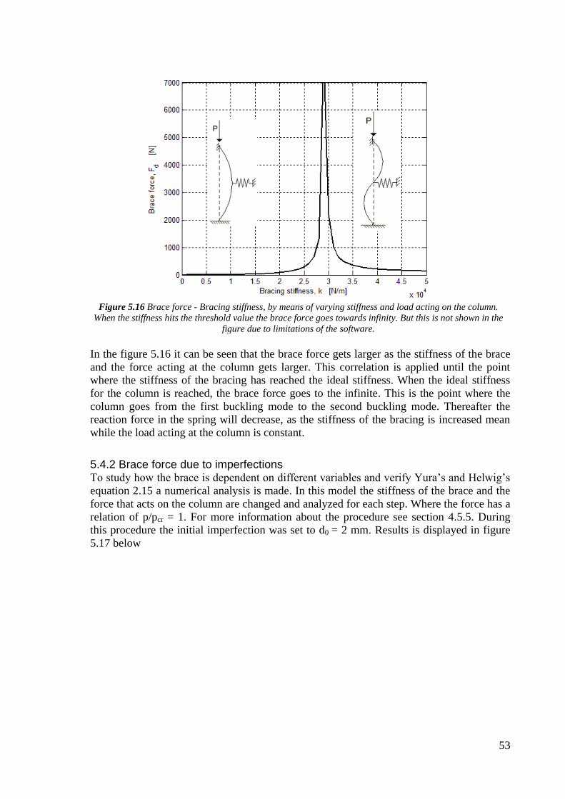
53
Figure 5.16 Brace force - Bracing stiffness, by means of varying stiffness and load acting on the column.
When the stiffness hits the threshold value the brace force goes towards infinity. But this is not shown in the
figure due to limitations of the software.
In the figure 5.16 it can be seen that the brace force gets larger as the stiffness of the brace
and the force acting at the column gets larger. This correlation is applied until the point
where the stiffness of the bracing has reached the ideal stiffness. When the ideal stiffness
for the column is reached, the brace force goes to the infinite. This is the point where the
column goes from the first buckling mode to the second buckling mode. Thereafter the
reaction force in the spring will decrease, as the stiffness of the bracing is increased mean
while the load acting at the column is constant.
5.4.2 Brace force due to imperfections To study how the brace is dependent on different variables and verify Yura’s and Helwig’s
equation 2.15 a numerical analysis is made. In this model the stiffness of the brace and the
force that acts on the column are changed and analyzed for each step. Where the force has a
relation of p/pcr = 1. For more information about the procedure see section 4.5.5. During
this procedure the initial imperfection was set to d0 = 2 mm. Results is displayed in figure
5.17 below
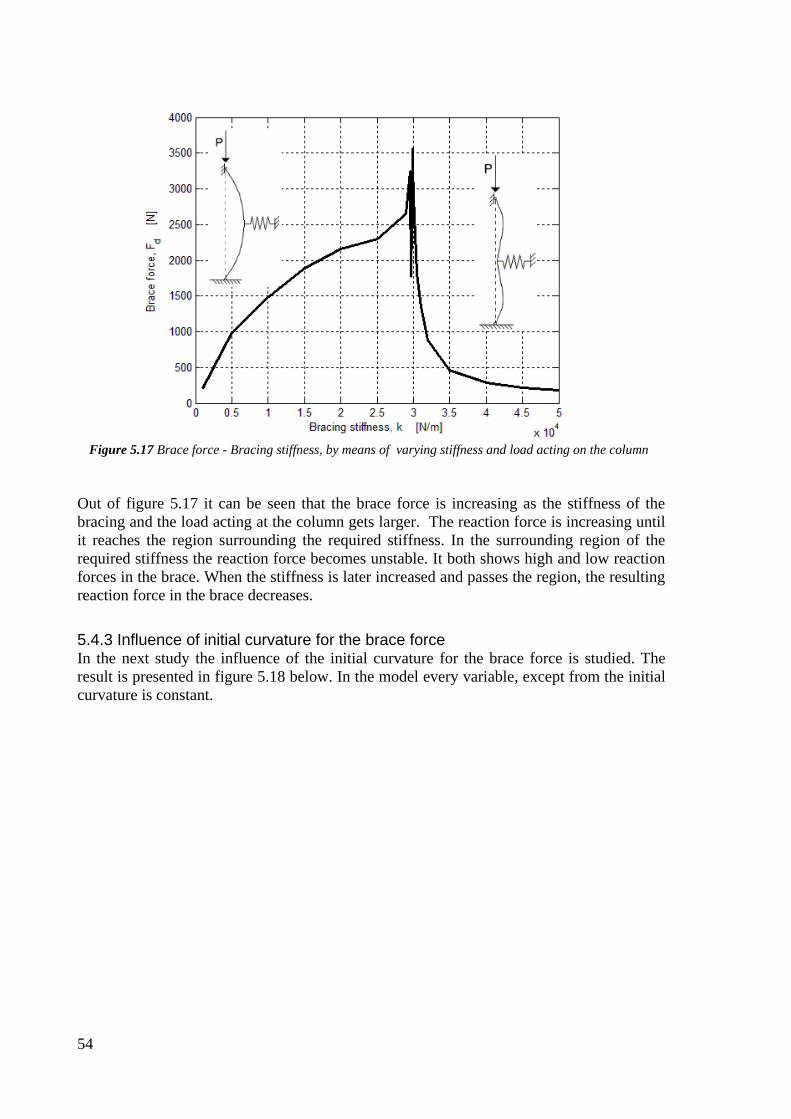
54
Figure 5.17 Brace force - Bracing stiffness, by means of varying stiffness and load acting on the column
Out of figure 5.17 it can be seen that the brace force is increasing as the stiffness of the
bracing and the load acting at the column gets larger. The reaction force is increasing until
it reaches the region surrounding the required stiffness. In the surrounding region of the
required stiffness the reaction force becomes unstable. It both shows high and low reaction
forces in the brace. When the stiffness is later increased and passes the region, the resulting
reaction force in the brace decreases.
5.4.3 Influence of initial curvature for the brace force In the next study the influence of the initial curvature for the brace force is studied. The
result is presented in figure 5.18 below. In the model every variable, except from the initial
curvature is constant.
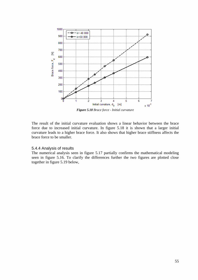
55
Figure 5.18 Brace force - Initial curvature
The result of the initial curvature evaluation shows a linear behavior between the brace
force due to increased initial curvature. In figure 5.18 it is shown that a larger initial
curvature leads to a higher brace force. It also shows that higher brace stiffness affects the
brace force to be smaller.
5.4.4 Analysis of results The numerical analysis seen in figure 5.17 partially confirms the mathematical modeling
seen in figure 5.16. To clarify the differences further the two figures are plotted close
together in figure 5.19 below,
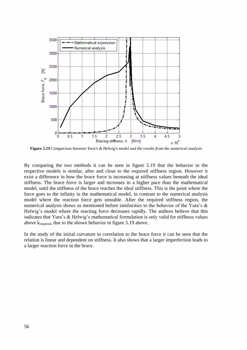
56
Figure 5.19 Comparison between Yura's & Helwig's model and the results from the numerical analysis
By comparing the two methods it can be seen in figure 5.19 that the behavior in the
respective models is similar, after and close to the required stiffness region. However it
exist a difference in how the brace force is increasing at stiffness values beneath the ideal
stiffness. The brace force is larger and increases in a higher pace than the mathematical
model, until the stiffness of the brace reaches the ideal stiffness. This is the point where the
force goes to the infinity in the mathematical model, in contrast to the numerical analysis
model where the reaction force gets unstable. After the required stiffness region, the
numerical analysis shows as mentioned before similarities to the behavior of the Yura’s &
Helwig’s model where the reacting force decreases rapidly. The authors believe that this
indicates that Yura’s & Helwig’s mathematical formulation is only valid for stiffness values
above krequired, due to the shown behavior in figure 5.19 above.
In the study of the initial curvature in correlation to the brace force it can be seen that the
relation is linear and dependent on stiffness. It also shows that a larger imperfection leads to
a larger reaction force in the brace.
57
6 Discussion and Conclusions
In this chapter the authors present the conclusions of the findings from the result and
analysis part in the previous chapter in this report.
Comparison between Eurocode and the U.S. Building code
In the start the main objective in this comparison was to study and clarify the difference
between Eurocode and the U.S. building code. But as the process went on, it was made
clear for the authors that the both standards couldn’t be compared due to the design of
respective standard.
The main difference between the two is that Eurocode uses the Ultimate Limite State
design (ULS) approach and that the U.S. building code is in use of allowable stresses. The
result of the two standards is therefore not comparable, as one can see in table 5.1, the load
bearing capacity of the two standards differs a lot. This information was unfortunately
revealed late for the authors.
If one were to analyze the result, one would think that the U.S. building code is more
restrictive for slender columns than Eurocode, and that Eurocode is more restrictive as the
column gets more robust.
Since time was running short a compromise had to be made, whereas the two building
standards were both faced with the same design problem. A comparison between the two
revealed that the U.S building code seem to be more restrictive than Eurocode, since
Eurocode always have the smaller cross-section of the two.
Influence of initial curvature
In the study it is shown that an initial curvature in a column will affect the overall load
bearing capacity. Initial curvature has a negative effect on the column, since it decreases its
total load bearing capacity. The reduction is dependent on the how large the magnitude of
the initial curvature is. It is shown in the result that a larger initial curvature will lead to
larger reduction of the load bearing capacity of the column, which was expected by the
authors.
It’s not only the load bearing capacity of the column that is affected by the initial curvature.
The total deformation and deformation rate is also affected by it. The findings show that the
total deformation and the deformation rate are increased, as the magnitude of the initial
curvature in the column gets larger.
The results were based on a simplified shape model of the initial curvature, whereas the
first buckling mode is the only one to affect the initial curvature. In reality the initial
curvature is a coalition of several different buckling modes, therefore the shape and
appearance of the initial curvature needs to be readjusted to a more plausible shape.
The findings indicates that if a correlation of the buckling modes is taken into account the
total load bearing capacity of the column will decrease compared to the simplified
imperfection model. The magnitude of the additional reduction on the load bearing capacity
of the column is however dependent on the resulting shape of the imperfection.
58
The study indicates that when higher tiers of the buckling modes govern the shape of the
initial curvature, the overall load bearing capacity will decrease further. The load bearing
capacity can with other words vary, dependent on the model one assume. The findings
indicate that the most disadvantageous situation for a column occurs when the higher
buckling shapes acquire its largest allowed amplitude.
Influence of brace stiffness
It is shown in the study that the stiffness of a brace has a contribution to the total load
bearing capacity of the column. The contribution is in an ideal column case proportional to
the increase in stiffness. Even though the increase is small, the increase is always present as
long as the stiffness is above zero. However, as the results shows there is a limit on how
much the load bearing capacity can be increased. As the stiffness of the brace reaches the
threshold value kideal a new buckling shape occurs, which will govern the load bearing
capacity. The load bearing capacity cannot thereafter be increased further.
By using additional braces the results shows that the column’s load bearing capacity can be
increased further. Dependent on the total amount of braces that are in use, the increase of
load bearing capacity will vary. However there exists a limit/ where it isn’t profitable to add
more braces. When this limit is reached the material capacity of the column will govern the
failure.
The study was continued with comparing the influence on a varying brace stiffness of
multiple braces, As mentioned before, the study indicates that an increase of brace stiffness
will result in a larger load bearing capacity. However as the stiffness of respective brace is
varied, the findings shows that there may exist a more favorable correlation between the
braces, if one is restricted.
But something the authors found was interesting was how a varying stiffness of respective
brace influenced on the total load bearing capacity for the column. It is revealed in the
result that even though a more robust brace lead to an increase in load bearing capacity for
the column, there are good things to keep in mind when designing the braces. It appears to
exist strategically places where one brace is more suitable than two/three less strategically
placed braces, when one has insufficient brace stiffness. A rule of thumb should be to
minimize the effective length of the column as much as possible. As in the case with three
braces, it is for example smarter to put a stiffer brace in the midpoint of the column with
two supporting braces at the sides.
The design guidance for a column’s brace stiffness in Eurocode isn’t as absolute, as in
Yura’s and Helwig’s model. As shown in the results, the brace stiffness can vary due the ks
factor one can choose in Eurocode. The study has shown that a smaller stiffness contributes
to a larger load bearing capacity. Eurocode does not calculate stiffness contribution per say,
it checks if the stiffness of the brace is rigid enough to be considered as a lateral support or
not. The authors think Eurocode should therefore be reevaluated in order to take into
account contributions from braces with a smaller stiffness.
Reaction force in a brace
This study shows that the brace force increases proportionally to the columns imperfection,
due to its dependence on the columns overall deformation. This correlation does only
coincide as the brace stiffness goes towards the required stiffness of the column, to make it

59
change its buckling shape. As the brace stiffness either become lesser or larger than the
required stiffness value, the brace force will decrease.
In the findings it is also shown that the numerical analysis has a large similarity to Yura’s
and Helwig’s mathematical model. However Yura’s and Helwig’s model is questioned, due
to its large difference in the area where the brace stiffness values is lower than Kreq. The
authors believes that the mathematical model of Yura and Helwig is only applicable for
describing correlations for a brace force that has brace stiffness larger than Kreq.

60
61
7 References
Books Bauchau, O. A., Craig, J. I. (2009), Structural analysis: With Applications to Aerospace
Structures. Dordrecht : Springer Netherlands
Breyer, Donald E. (2003). Design of wood structures ASD. 5. ed. New York: McGraw-Hill
Burström, Per Gunnar (2007). Byggnadsmaterial: uppbyggnad, tillverkning och
egenskaper. 2. uppl. Lund: Studentlitteratur
Galambos, Theodore V. & Surovek, Andrea (2008). Structural stability of steel: concepts
and applications for structural engineers. Hoboken, N.J.: John Wiley & Sons
Helwig, Todd A. & Yura, Joseph A. (1996), Bracing for stability, University of Houston
and University of Texas at Austin
Isaksson, Tord & Mårtensson, Annika (2010). Byggkonstruktion: regel- och formelsamling
: based on Eurokod. 2. ed. Lund: Studentlitteratur
Runesson, Kenneth, Samuelsson, Alf & Wiberg, Nils-Erik (1992).Byggnadsmekanik -
knäckning. Lund: Studentlitteratur
Stålbyggnadskommité (1973). Knäckning, vippning, buckling: kommentarer till
Stålbyggnadsnorm 70. Stockholm
Timoshenko, Stephen & Gere, James M. (1961). Theory of elastic stability. 2., rev. ed. New
York: McGraw-Hill
Trahair, Nicholas S. & Bradford, M. A. (1994). The behaviour and design of steel
structures. Rev. 2. ed. London: Spon
Winter, G. (1958). Lateral bracing of columns and beams , Proc. ASCE, 84, pp. 561–1561
(ST2)
Yura, J. (1996). Winter's bracing approach revisited. Engineering Structures Volume: 18
Issue: 10 (1996-10-01) p. 821 - 825.
Elektronic available literature: efunda. 2014, Columns: Introduction. [Electronic] Article
Engineering Fundamentals. Available:
<http://www.efunda.com/formulae/solid_mechanics/columns/intro.cfm> (2014-04-07)
ICC. 2014, Chapter 16: Structural Design. [Electronic] Part of book
Internation Code Council. Available:
<http://www2.iccsafe.org/states/newyorkcity/Building/PDFs/Chapter%2016_Structural%20
Design.pdf>

62
63
Appendix A – Unit Converter This Appendix is a reference document to convert U.S. costumary units into SI- units.
Loads
1 Ib = 4,448 N
1 k = 4,448 kN
Modulus of elasticity and stresses 1 psi = 6,895 kPA