Embed Size (px)
Citation preview

SPSS Classification Trees™ 16.0

For more information about SPSS® software products, please visit our Web site at http://www.spss.com or contact
SPSS Inc.233 South Wacker Drive, 11th FloorChicago, IL 60606-6412Tel: (312) 651-3000Fax: (312) 651-3668
SPSS is a registered trademark and the other product names are the trademarks of SPSS Inc. for its proprietary computer software. No materialdescribing such software may be produced or distributed without the written permission of the owners of the trademark and license rights in thesoftware and the copyrights in the published materials.
The SOFTWARE and documentation are provided with RESTRICTED RIGHTS. Use, duplication, or disclosure by the Government issubject to restrictions as set forth in subdivision (c) (1) (ii) of The Rights in Technical Data and Computer Software clause at 52.227-7013.Contractor/manufacturer is SPSS Inc., 233 South Wacker Drive, 11th Floor, Chicago, IL 60606-6412.Patent No. 7,023,453
General notice: Other product names mentioned herein are used for identification purposes only and may be trademarks of their respectivecompanies.
Windows is a registered trademark of Microsoft Corporation.
Apple, Mac, and the Mac logo are trademarks of Apple Computer, Inc., registered in the U.S. and other countries.
This product uses WinWrap Basic, Copyright 1993-2007, Polar Engineering and Consulting, http://www.winwrap.com.
SPSS Classification Trees™ 16.0Copyright © 2007 by SPSS Inc.All rights reserved.Printed in the United States of America.
No part of this publication may be reproduced, stored in a retrieval system, or transmitted, in any form or by any means, electronic, mechanical,photocopying, recording, or otherwise, without the prior written permission of the publisher.
1 2 3 4 5 6 7 8 9 0 10 09 08 07

Preface
SPSS 16.0 is a comprehensive system for analyzing data. The SPSS Classification Treesoptional add-on module provides the additional analytic techniques described in this manual.The Classification Trees add-on module must be used with the SPSS 16.0 Base system and iscompletely integrated into that system.
Installation
To install the SPSS Classification Trees add-on module, run the License Authorization Wizardusing the authorization code that you received from SPSS Inc. For more information, see theinstallation instructions supplied with the SPSS Classification Trees add-on module.
Compatibility
SPSS is designed to run on many computer systems. See the installation instructions that camewith your system for specific information on minimum and recommended requirements.
Serial Numbers
Your serial number is your identification number with SPSS Inc. You will need this serial numberwhen you contact SPSS Inc. for information regarding support, payment, or an upgraded system.The serial number was provided with your Base system.
Customer Service
If you have any questions concerning your shipment or account, contact your local office, listedon the SPSS Web site at http://www.spss.com/worldwide. Please have your serial number readyfor identification.
Training Seminars
SPSS Inc. provides both public and onsite training seminars. All seminars featurehands-on workshops. Seminars will be offered in major cities on a regular basis. For moreinformation on these seminars, contact your local office, listed on the SPSS Web site athttp://www.spss.com/worldwide.
Technical Support
The services of SPSS Technical Support are available to maintenance customers. Customersmay contact Technical Support for assistance in using SPSS or for installation help for oneof the supported hardware environments. To reach Technical Support, see the SPSS Web
iii

site at http://www.spss.com, or contact your local office, listed on the SPSS Web site athttp://www.spss.com/worldwide. Be prepared to identify yourself, your organization, and theserial number of your system.
Additional Publications
Additional copies of product manuals may be purchased directly from SPSS Inc. Visit the SPSSWeb Store at http://www.spss.com/estore, or contact your local SPSS office, listed on the SPSSWeb site at http://www.spss.com/worldwide. For telephone orders in the United States andCanada, call SPSS Inc. at 800-543-2185. For telephone orders outside of North America, contactyour local office, listed on the SPSS Web site.The SPSS Statistical Procedures Companion, by Marija Norušis, has been published by
Prentice Hall. A new version of this book, updated for SPSS 16.0, is planned. The SPSSAdvanced Statistical Procedures Companion, also based on SPSS 16.0, is forthcoming. TheSPSS Guide to Data Analysis for SPSS 16.0 is also in development. Announcements ofpublications available exclusively through Prentice Hall will be available on the SPSS Web site athttp://www.spss.com/estore (select your home country, and then click Books).
Tell Us Your Thoughts
Your comments are important. Please let us know about your experiences with SPSS products.We especially like to hear about new and interesting applications using the SPSS ClassificationTrees add-on module. Please send e-mail to [email protected] or write to SPSS Inc., Attn.:Director of Product Planning, 233 South Wacker Drive, 11th Floor, Chicago, IL 60606-6412.
About This Manual
This manual documents the graphical user interface for the procedures included in the SPSSClassification Trees add-on module. Illustrations of dialog boxes are taken from SPSS. Detailedinformation about the command syntax for features in the SPSS Classification Trees add-onmodule is available in two forms: integrated into the overall Help system and as a separatedocument in PDF form in the SPSS 16.0 Command Syntax Reference, available from the Helpmenu.
Contacting SPSS
If you would like to be on our mailing list, contact one of our offices, listed on our Web siteat http://www.spss.com/worldwide.
iv

Contents
1 Creating Classification Trees 1
Selecting Categories . . . . . . . . . . . . . . . . . . . . . . . . . . . . . . . . . . . . . . . . . . . . . . . . . . . . . . . . . . 6Validation . . . . . . . . . . . . . . . . . . . . . . . . . . . . . . . . . . . . . . . . . . . . . . . . . . . . . . . . . . . . . . . . . . . 7Tree-Growing Criteria . . . . . . . . . . . . . . . . . . . . . . . . . . . . . . . . . . . . . . . . . . . . . . . . . . . . . . . . . . 8
Growth Limits . . . . . . . . . . . . . . . . . . . . . . . . . . . . . . . . . . . . . . . . . . . . . . . . . . . . . . . . . . . . 9CHAID Criteria . . . . . . . . . . . . . . . . . . . . . . . . . . . . . . . . . . . . . . . . . . . . . . . . . . . . . . . . . . . . 10CRT Criteria . . . . . . . . . . . . . . . . . . . . . . . . . . . . . . . . . . . . . . . . . . . . . . . . . . . . . . . . . . . . . . 12QUEST Criteria. . . . . . . . . . . . . . . . . . . . . . . . . . . . . . . . . . . . . . . . . . . . . . . . . . . . . . . . . . . . 13Pruning Trees . . . . . . . . . . . . . . . . . . . . . . . . . . . . . . . . . . . . . . . . . . . . . . . . . . . . . . . . . . . . 14Surrogates . . . . . . . . . . . . . . . . . . . . . . . . . . . . . . . . . . . . . . . . . . . . . . . . . . . . . . . . . . . . . . 15
Options. . . . . . . . . . . . . . . . . . . . . . . . . . . . . . . . . . . . . . . . . . . . . . . . . . . . . . . . . . . . . . . . . . . . . 15Misclassification Costs . . . . . . . . . . . . . . . . . . . . . . . . . . . . . . . . . . . . . . . . . . . . . . . . . . . . . 16Profits . . . . . . . . . . . . . . . . . . . . . . . . . . . . . . . . . . . . . . . . . . . . . . . . . . . . . . . . . . . . . . . . . . 17Prior Probabilities . . . . . . . . . . . . . . . . . . . . . . . . . . . . . . . . . . . . . . . . . . . . . . . . . . . . . . . . . 18Scores. . . . . . . . . . . . . . . . . . . . . . . . . . . . . . . . . . . . . . . . . . . . . . . . . . . . . . . . . . . . . . . . . . 20Missing Values . . . . . . . . . . . . . . . . . . . . . . . . . . . . . . . . . . . . . . . . . . . . . . . . . . . . . . . . . . . 21
Saving Model Information. . . . . . . . . . . . . . . . . . . . . . . . . . . . . . . . . . . . . . . . . . . . . . . . . . . . . . . 22Output . . . . . . . . . . . . . . . . . . . . . . . . . . . . . . . . . . . . . . . . . . . . . . . . . . . . . . . . . . . . . . . . . . . . . 23
Tree Display. . . . . . . . . . . . . . . . . . . . . . . . . . . . . . . . . . . . . . . . . . . . . . . . . . . . . . . . . . . . . . 24Statistics . . . . . . . . . . . . . . . . . . . . . . . . . . . . . . . . . . . . . . . . . . . . . . . . . . . . . . . . . . . . . . . . 26Charts . . . . . . . . . . . . . . . . . . . . . . . . . . . . . . . . . . . . . . . . . . . . . . . . . . . . . . . . . . . . . . . . . . 29Selection and Scoring Rules . . . . . . . . . . . . . . . . . . . . . . . . . . . . . . . . . . . . . . . . . . . . . . . . . 35
2 Tree Editor 37
Working with Large Trees . . . . . . . . . . . . . . . . . . . . . . . . . . . . . . . . . . . . . . . . . . . . . . . . . . . . . . . 38Tree Map . . . . . . . . . . . . . . . . . . . . . . . . . . . . . . . . . . . . . . . . . . . . . . . . . . . . . . . . . . . . . . . . 39Scaling the Tree Display . . . . . . . . . . . . . . . . . . . . . . . . . . . . . . . . . . . . . . . . . . . . . . . . . . . . 39Node Summary Window . . . . . . . . . . . . . . . . . . . . . . . . . . . . . . . . . . . . . . . . . . . . . . . . . . . . 40
Controlling Information Displayed in the Tree . . . . . . . . . . . . . . . . . . . . . . . . . . . . . . . . . . . . . . . . 41Changing Tree Colors and Text Fonts. . . . . . . . . . . . . . . . . . . . . . . . . . . . . . . . . . . . . . . . . . . . . . . 42Case Selection and Scoring Rules . . . . . . . . . . . . . . . . . . . . . . . . . . . . . . . . . . . . . . . . . . . . . . . . 44
Filtering Cases . . . . . . . . . . . . . . . . . . . . . . . . . . . . . . . . . . . . . . . . . . . . . . . . . . . . . . . . . . . . 44Saving Selection and Scoring Rules. . . . . . . . . . . . . . . . . . . . . . . . . . . . . . . . . . . . . . . . . . . . 45
v

3 Data Assumptions and Requirements 47
Effects of Measurement Level on Tree Models . . . . . . . . . . . . . . . . . . . . . . . . . . . . . . . . . . . . . . . 47Permanently Assigning Measurement Level. . . . . . . . . . . . . . . . . . . . . . . . . . . . . . . . . . . . . . 50
Effects of Value Labels on Tree Models. . . . . . . . . . . . . . . . . . . . . . . . . . . . . . . . . . . . . . . . . . . . . 51Assigning Value Labels to All Values . . . . . . . . . . . . . . . . . . . . . . . . . . . . . . . . . . . . . . . . . . . 52
4 Using Classification Trees to Evaluate Credit Risk 54
Creating the Model . . . . . . . . . . . . . . . . . . . . . . . . . . . . . . . . . . . . . . . . . . . . . . . . . . . . . . . . . . . . 54Building the CHAID Tree Model . . . . . . . . . . . . . . . . . . . . . . . . . . . . . . . . . . . . . . . . . . . . . . . 54Selecting Target Categories. . . . . . . . . . . . . . . . . . . . . . . . . . . . . . . . . . . . . . . . . . . . . . . . . . 55Specifying Tree Growing Criteria . . . . . . . . . . . . . . . . . . . . . . . . . . . . . . . . . . . . . . . . . . . . . . 56Selecting Additional Output . . . . . . . . . . . . . . . . . . . . . . . . . . . . . . . . . . . . . . . . . . . . . . . . . . 57Saving Predicted Values . . . . . . . . . . . . . . . . . . . . . . . . . . . . . . . . . . . . . . . . . . . . . . . . . . . . 59
Evaluating the Model . . . . . . . . . . . . . . . . . . . . . . . . . . . . . . . . . . . . . . . . . . . . . . . . . . . . . . . . . . 60Model Summary Table . . . . . . . . . . . . . . . . . . . . . . . . . . . . . . . . . . . . . . . . . . . . . . . . . . . . . . 61Tree Diagram . . . . . . . . . . . . . . . . . . . . . . . . . . . . . . . . . . . . . . . . . . . . . . . . . . . . . . . . . . . . . 62Tree Table . . . . . . . . . . . . . . . . . . . . . . . . . . . . . . . . . . . . . . . . . . . . . . . . . . . . . . . . . . . . . . . 63Gains for Nodes. . . . . . . . . . . . . . . . . . . . . . . . . . . . . . . . . . . . . . . . . . . . . . . . . . . . . . . . . . . 64Gains Chart . . . . . . . . . . . . . . . . . . . . . . . . . . . . . . . . . . . . . . . . . . . . . . . . . . . . . . . . . . . . . . 65Index Chart . . . . . . . . . . . . . . . . . . . . . . . . . . . . . . . . . . . . . . . . . . . . . . . . . . . . . . . . . . . . . . 65Risk Estimate and Classification. . . . . . . . . . . . . . . . . . . . . . . . . . . . . . . . . . . . . . . . . . . . . . . 66Predicted Values . . . . . . . . . . . . . . . . . . . . . . . . . . . . . . . . . . . . . . . . . . . . . . . . . . . . . . . . . . 67
Refining the Model . . . . . . . . . . . . . . . . . . . . . . . . . . . . . . . . . . . . . . . . . . . . . . . . . . . . . . . . . . . . 68Selecting Cases in Nodes . . . . . . . . . . . . . . . . . . . . . . . . . . . . . . . . . . . . . . . . . . . . . . . . . . . 68Examining the Selected Cases . . . . . . . . . . . . . . . . . . . . . . . . . . . . . . . . . . . . . . . . . . . . . . . . 69Assigning Costs to Outcomes. . . . . . . . . . . . . . . . . . . . . . . . . . . . . . . . . . . . . . . . . . . . . . . . . 72
Summary . . . . . . . . . . . . . . . . . . . . . . . . . . . . . . . . . . . . . . . . . . . . . . . . . . . . . . . . . . . . . . . . . . . 76
5 Building a Scoring Model 77
Building the Model . . . . . . . . . . . . . . . . . . . . . . . . . . . . . . . . . . . . . . . . . . . . . . . . . . . . . . . . . . . . 77Evaluating the Model . . . . . . . . . . . . . . . . . . . . . . . . . . . . . . . . . . . . . . . . . . . . . . . . . . . . . . . . . . 80
Model Summary . . . . . . . . . . . . . . . . . . . . . . . . . . . . . . . . . . . . . . . . . . . . . . . . . . . . . . . . . . 80Tree Model Diagram . . . . . . . . . . . . . . . . . . . . . . . . . . . . . . . . . . . . . . . . . . . . . . . . . . . . . . . 81Risk Estimate . . . . . . . . . . . . . . . . . . . . . . . . . . . . . . . . . . . . . . . . . . . . . . . . . . . . . . . . . . . . . 82
Applying the Model to Another Data File . . . . . . . . . . . . . . . . . . . . . . . . . . . . . . . . . . . . . . . . . . . . 83Summary . . . . . . . . . . . . . . . . . . . . . . . . . . . . . . . . . . . . . . . . . . . . . . . . . . . . . . . . . . . . . . . . . . . 86
vi

6 Missing Values in Tree Models 87
Missing Values with CHAID . . . . . . . . . . . . . . . . . . . . . . . . . . . . . . . . . . . . . . . . . . . . . . . . . . . . . 88CHAID Results . . . . . . . . . . . . . . . . . . . . . . . . . . . . . . . . . . . . . . . . . . . . . . . . . . . . . . . . . . . . 90
Missing Values with CRT. . . . . . . . . . . . . . . . . . . . . . . . . . . . . . . . . . . . . . . . . . . . . . . . . . . . . . . . 91CRT Results . . . . . . . . . . . . . . . . . . . . . . . . . . . . . . . . . . . . . . . . . . . . . . . . . . . . . . . . . . . . . . 94
Summary . . . . . . . . . . . . . . . . . . . . . . . . . . . . . . . . . . . . . . . . . . . . . . . . . . . . . . . . . . . . . . . . . . . 96
Appendix
A Sample Files 97
Index 107
vii


Chapter
1Creating Classification Trees
Figure 1-1Classification tree
The Classification Tree procedure creates a tree-based classification model. It classifies casesinto groups or predicts values of a dependent (target) variable based on values of independent(predictor) variables. The procedure provides validation tools for exploratory and confirmatoryclassification analysis.
The procedure can be used for:
Segmentation. Identify persons who are likely to be members of a particular group.
Stratification. Assign cases into one of several categories, such as high-, medium-, and low-riskgroups.
1

2
Chapter 1
Prediction. Create rules and use them to predict future events, such as the likelihood that someonewill default on a loan or the potential resale value of a vehicle or home.
Data reduction and variable screening. Select a useful subset of predictors from a large set ofvariables for use in building a formal parametric model.
Interaction identification. Identify relationships that pertain only to specific subgroups and specifythese in a formal parametric model.
Category merging and discretizing continuous variables. Recode group predictor categories andcontinuous variables with minimal loss of information.
Example. A bank wants to categorize credit applicants according to whether or not they representa reasonable credit risk. Based on various factors, including the known credit ratings of pastcustomers, you can build a model to predict if future customers are likely to default on their loans.
A tree-based analysis provides some attractive features:It allows you to identify homogeneous groups with high or low risk.It makes it easy to construct rules for making predictions about individual cases.
Data Considerations
Data. The dependent and independent variables can be:Nominal. A variable can be treated as nominal when its values represent categories with nointrinsic ranking (for example, the department of the company in which an employee works).Examples of nominal variables include region, zip code, and religious affiliation.Ordinal. A variable can be treated as ordinal when its values represent categories with someintrinsic ranking (for example, levels of service satisfaction from highly dissatisfied tohighly satisfied). Examples of ordinal variables include attitude scores representing degreeof satisfaction or confidence and preference rating scores.Scale. A variable can be treated as scale when its values represent ordered categories with ameaningful metric, so that distance comparisons between values are appropriate. Examples ofscale variables include age in years and income in thousands of dollars.
Frequency weights If weighting is in effect, fractional weights are rounded to the closest integer;so, cases with a weight value of less than 0.5 are assigned a weight of 0 and are therefore excludedfrom the analysis.
Assumptions. This procedure assumes that the appropriate measurement level has been assignedto all analysis variables, and some features assume that all values of the dependent variableincluded in the analysis have defined value labels.
Measurement level. Measurement level affects the tree computations; so, all variables shouldbe assigned the appropriate measurement level. By default, numeric variables are assumed tobe scale and string variables are assumed to be nominal, which may not accurately reflect

3
Creating Classification Trees
the true measurement level. An icon next to each variable in the variable list identifies thevariable type.
Scale
Nominal
Ordinal
You can temporarily change the measurement level for a variable by right-clicking the variable inthe source variable list and selecting a measurement level from the context menu.
Value labels. The dialog box interface for this procedure assumes that either all nonmissingvalues of a categorical (nominal, ordinal) dependent variable have defined value labels ornone of them do. Some features are not available unless at least two nonmissing valuesof the categorical dependent variable have value labels. If at least two nonmissing valueshave defined value labels, any cases with other values that do not have value labels will beexcluded from the analysis.
To Obtain Classification Trees
E From the menus choose:Analyze
ClassifyTree...

4
Chapter 1
Figure 1-2Classification Tree dialog box
E Select a dependent variable.
E Select one or more independent variables.
E Select a growing method.
Optionally, you can:Change the measurement level for any variable in the source list.Force the first variable in the independent variables list into the model as the first split variable.Select an influence variable that defines how much influence a case has on the tree-growingprocess. Cases with lower influence values have less influence; cases with higher values havemore. Influence variable values must be positive.Validate the tree.Customize the tree-growing criteria.Save terminal node numbers, predicted values, and predicted probabilities as variables.Save the model in XML (PMML) format.
Changing Measurement Level
E Right-click the variable in the source list.
E Select a measurement level from the pop-up context menu.
This changes the measurement level temporarily for use in the Classification Tree procedure.

5
Creating Classification Trees
Growing Methods
The available growing methods are:
CHAID. Chi-squared Automatic Interaction Detection. At each step, CHAID chooses theindependent (predictor) variable that has the strongest interaction with the dependent variable.Categories of each predictor are merged if they are not significantly different with respect to thedependent variable.
Exhaustive CHAID.A modification of CHAID that examines all possible splits for each predictor.
CRT. Classification and Regression Trees. CRT splits the data into segments that are ashomogeneous as possible with respect to the dependent variable. A terminal node in which allcases have the same value for the dependent variable is a homogeneous, "pure" node.
QUEST. Quick, Unbiased, Efficient Statistical Tree. A method that is fast and avoids othermethods’ bias in favor of predictors with many categories. QUEST can be specified only ifthe dependent variable is nominal.
There are benefits and limitations with each method, including:
CHAID* CRT QUESTChi-square-based** XSurrogate independent (predictor)variables
X X
Tree pruning X XMultiway node splitting XBinary node splitting X XInfluence variables X XPrior probabilities X XMisclassification costs X X XFast calculation X X
*Includes Exhaustive CHAID.
**QUEST also uses a chi-square measure for nominal independent variables.

6
Chapter 1
Selecting CategoriesFigure 1-3Categories dialog box
For categorical (nominal, ordinal) dependent variables, you can:Control which categories are included in the analysis.Identify the target categories of interest.
Including/Excluding Categories
You can limit the analysis to specific categories of the dependent variable.Cases with values of the dependent variable in the Exclude list are not included in the analysis.For nominal dependent variables, you can also include user-missing categories in the analysis.(By default, user-missing categories are displayed in the Exclude list.)
Target Categories
Selected (checked) categories are treated as the categories of primary interest in the analysis. Forexample, if you are primarily interested in identifying those individuals most likely to default on aloan, you might select the “bad” credit-rating category as the target category.
There is no default target category. If no category is selected, some classification rule optionsand gains-related output are not available.If multiple categories are selected, separate gains tables and charts are produced for eachtarget category.Designating one or more categories as target categories has no effect on the tree model, riskestimate, or misclassification results.

7
Creating Classification Trees
Categories and Value Labels
This dialog box requires defined value labels for the dependent variable. It is not available unlessat least two values of the categorical dependent variable have defined value labels.
To Include/Exclude Categories and Select Target Categories
E In the main Classification Tree dialog box, select a categorical (nominal, ordinal) dependentvariable with two or more defined value labels.
E Click Categories.
ValidationFigure 1-4Validation dialog box
Validation allows you to assess how well your tree structure generalizes to a larger population.Two validation methods are available: crossvalidation and split-sample validation.

8
Chapter 1
Crossvalidation
Crossvalidation divides the sample into a number of subsamples, or folds. Tree models are thengenerated, excluding the data from each subsample in turn. The first tree is based on all of thecases except those in the first sample fold, the second tree is based on all of the cases except thosein the second sample fold, and so on. For each tree, misclassification risk is estimated by applyingthe tree to the subsample excluded in generating it.
You can specify a maximum of 25 sample folds. The higher the value, the fewer the numberof cases excluded for each tree model.Crossvalidation produces a single, final tree model. The crossvalidated risk estimate for thefinal tree is calculated as the average of the risks for all of the trees.
Split-Sample Validation
With split-sample validation, the model is generated using a training sample and tested on ahold-out sample.
You can specify a training sample size, expressed as a percentage of the total sample size, or avariable that splits the sample into training and testing samples.If you use a variable to define training and testing samples, cases with a value of 1 for thevariable are assigned to the training sample, and all other cases are assigned to the testingsample. The variable cannot be the dependent variable, weight variable, influence variable,or a forced independent variable.You can display results for both the training and testing samples or just the testing sample.Split-sample validation should be used with caution on small data files (data files with a smallnumber of cases). Small training sample sizes may yield poor models, since there may not beenough cases in some categories to adequately grow the tree.
Tree-Growing Criteria
The available growing criteria may depend on the growing method, level of measurement of thedependent variable, or a combination of the two.

9
Creating Classification Trees
Growth LimitsFigure 1-5Criteria dialog box, Growth Limits tab
The Growth Limits tab allows you to limit the number of levels in the tree and control theminimum number of cases for parent and child nodes.
Maximum Tree Depth. Controls the maximum number of levels of growth beneath the root node.The Automatic setting limits the tree to three levels beneath the root node for the CHAID andExhaustive CHAID methods and five levels for the CRT and QUEST methods.
Minimum Number of Cases. Controls the minimum numbers of cases for nodes. Nodes that do notsatisfy these criteria will not be split.
Increasing the minimum values tends to produce trees with fewer nodes.Decreasing the minimum values produces trees with more nodes.
For data files with a small number of cases, the default values of 100 cases for parent nodes and 50cases for child nodes may sometimes result in trees with no nodes below the root node; in thiscase, lowering the minimum values may produce more useful results.

10
Chapter 1
CHAID CriteriaFigure 1-6Criteria dialog box, CHAID tab
For the CHAID and Exhaustive CHAID methods, you can control:
Significance Level. You can control the significance value for splitting nodes and mergingcategories. For both criteria, the default significance level is 0.05.
For splitting nodes, the value must be greater than 0 and less than 1. Lower values tend toproduce trees with fewer nodes.For merging categories, the value must be greater than 0 and less than or equal to 1. To preventmerging of categories, specify a value of 1. For a scale independent variable, this means thatthe number of categories for the variable in the final tree is the specified number of intervals(the default is 10). For more information, see Scale Intervals for CHAID Analysis on p. 11.
Chi-Square Statistic. For ordinal dependent variables, chi-square for determining node splittingand category merging is calculated using the likelihood-ratio method. For nominal dependentvariables, you can select the method:
Pearson. This method provides faster calculations but should be used with caution on smallsamples. This is the default method.Likelihood ratio. This method is more robust that Pearson but takes longer to calculate. Forsmall samples, this is the preferred method.
Model Estimation. For nominal and ordinal dependent variables, you can specify:Maximum number of iterations. The default is 100. If the tree stops growing because themaximum number of iterations has been reached, you may want to increase the maximum orchange one or more of the other criteria that control tree growth.Minimum change in expected cell frequencies. The value must be greater than 0 and less than1. The default is 0.05. Lower values tend to produce trees with fewer nodes.

11
Creating Classification Trees
Adjust significance values using Bonferroni method. For multiple comparisons, significance valuesfor merging and splitting criteria are adjusted using the Bonferroni method. This is the default.
Allow resplitting of merged categories within a node. Unless you explicitly prevent categorymerging, the procedure will attempt to merge independent (predictor) variable categories togetherto produce the simplest tree that describes the model. This option allows the procedure to resplitmerged categories if that provides a better solution.
Scale Intervals for CHAID Analysis
Figure 1-7Criteria dialog box, Intervals tab
In CHAID analysis, scale independent (predictor) variables are always banded into discrete groups(for example, 0–10, 11–20, 21–30, etc.) prior to analysis. You can control the initial/maximumnumber of groups (although the procedure may merge contiguous groups after the initial split):
Fixed number. All scale independent variables are initially banded into the same number ofgroups. The default is 10.Custom. Each scale independent variable is initially banded into the number of groupsspecified for that variable.
To Specify Intervals for Scale Independent Variables
E In the main Classification Tree dialog box, select one or more scale independent variables.
E For the growing method, select CHAID or Exhaustive CHAID.
E Click Criteria.
E Click the Intervals tab.

12
Chapter 1
In CRT and QUEST analysis, all splits are binary and scale and ordinal independent variablesare handled the same way; so, you cannot specify a number of intervals for scale independentvariables.
CRT CriteriaFigure 1-8Criteria dialog box, CRT tab
The CRT growing method attempts to maximize within-node homogeneity. The extent to which anode does not represent a homogenous subset of cases is an indication of impurity. For example,a terminal node in which all cases have the same value for the dependent variable is a homogenousnode that requires no further splitting because it is “pure.”You can select the method used to measure impurity and the minimum decrease in impurity
required to split nodes.
Impurity Measure. For scale dependent variables, the least-squared deviation (LSD) measure ofimpurity is used. It is computed as the within-node variance, adjusted for any frequency weightsor influence values.
For categorical (nominal, ordinal) dependent variables, you can select the impurity measure:Gini. Splits are found that maximize the homogeneity of child nodes with respect to thevalue of the dependent variable. Gini is based on squared probabilities of membership foreach category of the dependent variable. It reaches its minimum (zero) when all cases in anode fall into a single category. This is the default measure.Twoing. Categories of the dependent variable are grouped into two subclasses. Splits are foundthat best separate the two groups.Ordered twoing. Similar to twoing except that only adjacent categories can be grouped. Thismeasure is available only for ordinal dependent variables.
13
Creating Classification Trees
Minimum change in improvement. This is the minimum decrease in impurity required to split anode. The default is 0.0001. Higher values tend to produce trees with fewer nodes.
QUEST CriteriaFigure 1-9Criteria dialog box, QUEST tab
For the QUEST method, you can specify the significance level for splitting nodes. An independentvariable cannot be used to split nodes unless the significance level is less than or equal to thespecified value. The value must be greater than 0 and less than 1. The default is 0.05. Smallervalues will tend to exclude more independent variables from the final model.
To Specify QUEST Criteria
E In the main Classification Tree dialog box, select a nominal dependent variable.
E For the growing method, select QUEST.
E Click Criteria.
E Click the QUEST tab.

14
Chapter 1
Pruning TreesFigure 1-10Criteria dialog box, Pruning tab
With the CRT and QUEST methods, you can avoid overfitting the model by pruning the tree:the tree is grown until stopping criteria are met, and then it is trimmed automatically to thesmallest subtree based on the specified maximum difference in risk. The risk value is expressedin standard errors. The default is 1. The value must be non-negative. To obtain the subtreewith the minimum risk, specify 0.
Pruning versus Hiding Nodes
When you create a pruned tree, any nodes pruned from the tree are not available in the final tree.You can interactively hide and show selected child nodes in the final tree, but you cannot shownodes that were pruned in the tree creation process. For more information, see Tree Editor inChapter 2 on p. 37.

15
Creating Classification Trees
SurrogatesFigure 1-11Criteria dialog box, Surrogates tab
CRT and QUEST can use surrogates for independent (predictor) variables. For cases in which thevalue for that variable is missing, other independent variables having high associations with theoriginal variable are used for classification. These alternative predictors are called surrogates. Youcan specify the maximum number of surrogates to use in the model.
By default, the maximum number of surrogates is one less than the number of independentvariables. In other words, for each independent variable, all other independent variablesmay be used as surrogates.If you don’t want the model to use surrogates, specify 0 for the number of surrogates.
Options
Available options may depend on the growing method, the level of measurement of the dependentvariable, and/or the existence of defined value labels for values of the dependent variable.

16
Chapter 1
Misclassification CostsFigure 1-12Options dialog box, Misclassification Costs tab
For categorical (nominal, ordinal) dependent variables, misclassification costs allow you to includeinformation about the relative penalty associated with incorrect classification. For example:
The cost of denying credit to a creditworthy customer is likely to be different from the cost ofextending credit to a customer who then defaults on the loan.The cost of misclassifying an individual with a high risk of heart disease as low risk isprobably much higher than the cost of misclassifying a low-risk individual as high-risk.The cost of sending a mass mailing to someone who isn’t likely to respond is probably fairlylow, while the cost of not sending the mailing to someone who is likely to respond is relativelyhigher (in terms of lost revenue).
Misclassification Costs and Value Labels
This dialog box is not available unless at least two values of the categorical dependent variablehave defined value labels.
To Specify Misclassification Costs
E In the main Classification Tree dialog box, select a categorical (nominal, ordinal) dependentvariable with two or more defined value labels.
E Click Options.
E Click the Misclassification Costs tab.
E Click Custom.

17
Creating Classification Trees
E Enter one or more misclassification costs in the grid. Values must be non-negative. (Correctclassifications, represented on the diagonal, are always 0.)
Fill Matrix. In many instances, you may want costs to be symmetric—that is, the cost ofmisclassifying A as B is the same as the cost of misclassifying B as A. The following controls canmake it easier to specify a symmetric cost matrix:
Duplicate Lower Triangle. Copies values in the lower triangle of the matrix (below thediagonal) into the corresponding upper-triangular cells.Duplicate Upper Triangle. Copies values in the upper triangle of the matrix (above the diagonal)into the corresponding lower-triangular cells.Use Average Cell Values. For each cell in each half of the matrix, the two values (upper- andlower-triangular) are averaged and the average replaces both values. For example, if the costof misclassifying A as B is 1 and the cost of misclassifying B as A is 3, then this controlreplaces both of those values with the average (1+3)/2 = 2.
ProfitsFigure 1-13Options dialog box, Profits tab
For categorical dependent variables, you can assign revenue and expense values to levels of thedependent variable.
Profit is computed as revenue minus expense.Profit values affect average profit and ROI (return on investment) values in gains tables. Theydo not affect the basic tree model structure.Revenue and expense values must be numeric and must be specified for all categories ofthe dependent variable displayed in the grid.

18
Chapter 1
Profits and Value Labels
This dialog box requires defined value labels for the dependent variable. It is not available unlessat least two values of the categorical dependent variable have defined value labels.
To Specify Profits
E In the main Classification Tree dialog box, select a categorical (nominal, ordinal) dependentvariable with two or more defined value labels.
E Click Options.
E Click the Profits tab.
E Click Custom.
E Enter revenue and expense values for all dependent variable categories listed in the grid.
Prior ProbabilitiesFigure 1-14Options dialog box, Prior Probabilities tab
For CRT and QUEST trees with categorical dependent variables, you can specify priorprobabilities of group membership. Prior probabilities are estimates of the overall relativefrequency for each category of the dependent variable prior to knowing anything about the valuesof the independent (predictor) variables. Using prior probabilities helps to correct any tree growthcaused by data in the sample that is not representative of the entire population.

19
Creating Classification Trees
Obtain from training sample (empirical priors). Use this setting if the distribution of dependentvariable values in the data file is representative of the population distribution. If you are usingsplit-sample validation, the distribution of cases in the training sample is used.
Note: Since cases are randomly assigned to the training sample in split-sample validation,you won’t know the actual distribution of cases in the training sample in advance. For moreinformation, see Validation on p. 7.
Equal across categories. Use this setting if categories of the dependent variable are representedequally in the population. For example, if there are four categories, approximately 25% of thecases are in each category.
Custom. Enter a non-negative value for each category of the dependent variable listed in the grid.The values can be proportions, percentages, frequency counts, or any other values that representthe distribution of values across categories.
Adjust priors using misclassification costs. If you define custom misclassification costs, you canadjust prior probabilities based on those costs. For more information, see Misclassification Costson p. 16.
Profits and Value Labels
This dialog box requires defined value labels for the dependent variable. It is not available unlessat least two values of the categorical dependent variable have defined value labels.
To Specify Prior Probabilities
E In the main Classification Tree dialog box, select a categorical (nominal, ordinal) dependentvariable with two or more defined value labels.
E For the growing method, select CRT or QUEST.
E Click Options.
E Click the Prior Probabilities tab.

20
Chapter 1
Scores
Figure 1-15Options dialog box, Scores tab
For CHAID and Exhaustive CHAID with an ordinal dependent variable, you can assign customscores to each category of the dependent variable. Scores define the order of and distance betweencategories of the dependent variable. You can use scores to increase or decrease the relativedistance between ordinal values or to change the order of the values.
Use ordinal rank for each category. The lowest category of the dependent variable is assigned ascore of 1, the next highest category is assigned a score of 2, and so on. This is the default.Custom. Enter a numeric score value for each category of the dependent variable listed in thegrid.
Example
Value Label Original Value ScoreUnskilled 1 1Skilled manual 2 4Clerical 3 4.5Professional 4 7Management 5 6
The scores increase the relative distance between Unskilled and Skilled manual and decreasethe relative distance between Skilled manual and Clerical.The scores reverse the order of Management and Professional.

21
Creating Classification Trees
Scores and Value Labels
This dialog box requires defined value labels for the dependent variable. It is not available unlessat least two values of the categorical dependent variable have defined value labels.
To Specify Scores
E In the main Classification Tree dialog box, select an ordinal dependent variable with two ormore defined value labels.
E For the growing method, select CHAID or Exhaustive CHAID.
E Click Options.
E Click the Scores tab.
Missing ValuesFigure 1-16Options dialog box, Missing Values tab
The Missing Values tab controls the handling of nominal, user-missing, independent (predictor)variable values.
Handling of ordinal and scale user-missing independent variable values varies betweengrowing methods.Handling of nominal dependent variables is specified in the Categories dialog box. For moreinformation, see Selecting Categories on p. 6.For ordinal and scale dependent variables, cases with system-missing or user-missingdependent variable values are always excluded.

22
Chapter 1
Treat as missing values. User-missing values are treated like system-missing values. The handlingof system-missing values varies between growing methods.
Treat as valid values. User-missing values of nominal independent variables are treated as ordinaryvalues in tree growing and classification.
Method-Dependent Rules
If some, but not all, independent variable values are system- or user-missing:For CHAID and Exhaustive CHAID, system- and user-missing independent variable valuesare included in the analysis as a single, combined category. For scale and ordinal independentvariables, the algorithms first generate categories using valid values and then decide whetherto merge the missing category with its most similar (valid) category or keep it as a separatecategory.For CRT and QUEST, cases with missing independent variable values are excluded from thetree-growing process but are classified using surrogates if surrogates are included in themethod. If nominal user-missing values are treated as missing, they are also handled in thismanner. For more information, see Surrogates on p. 15.
To Specify Nominal, Independent User-Missing Treatment
E In the main Classification Tree dialog box, select at least one nominal independent variable.
E Click Options.
E Click the Missing Values tab.
Saving Model InformationFigure 1-17Save dialog box
You can save information from the model as variables in the working data file, and you can alsosave the entire model in XML (PMML) format to an external file.

23
Creating Classification Trees
Saved Variables
Terminal node number. The terminal node to which each case is assigned. The value is the treenode number.
Predicted value. The class (group) or value for the dependent variable predicted by the model.
Predicted probabilities. The probability associated with the model’s prediction. One variable issaved for each category of the dependent variable. Not available for scale dependent variables.
Sample assignment (training/testing). For split-sample validation, this variable indicates whethera case was used in the training or testing sample. The value is 1 for the training sample and 0for the testing sample. Not available unless you have selected split-sample validation. For moreinformation, see Validation on p. 7.
Export Tree Model as XML
You can save the entire tree model in XML (PMML) format. SmartScore and SPSS Server (aseparate product) can use this model file to apply the model information to other data files forscoring purposes.
Training sample. Writes the model to the specified file. For split-sample validated trees, this isthe model for the training sample.
Test sample. Writes the model for the test sample to the specified file. Not available unless youhave selected split-sample validation.
Output
Available output options depend on the growing method, the measurement level of the dependentvariable, and other settings.

24
Chapter 1
Tree DisplayFigure 1-18Output dialog box, Tree tab
You can control the initial appearance of the tree or completely suppress the tree display.
Tree. By default, the tree diagram is included in the output displayed in the Viewer. Deselect(uncheck) this option to exclude the tree diagram from the output.
Display. These options control the initial appearance of the tree diagram in the Viewer. All ofthese attributes can also be modified by editing the generated tree.
Orientation. The tree can be displayed top down with the root node at the top, left to right,or right to left.Node contents. Nodes can display tables, charts, or both. For categorical dependent variables,tables display frequency counts and percentages, and the charts are bar charts. For scaledependent variables, tables display means, standard deviations, number of cases, andpredicted values, and the charts are histograms.Scale. By default, large trees are automatically scaled down in an attempt to fit the tree on thepage. You can specify a custom scale percentage of up to 200%.Independent variable statistics. For CHAID and Exhaustive CHAID, statistics include F value(for scale dependent variables) or chi-square value (for categorical dependent variables)as well as significance value and degrees of freedom. For CRT, the improvement value isshown. For QUEST, F, significance value, and degrees of freedom are shown for scale and

25
Creating Classification Trees
ordinal independent variables; for nominal independent variables, chi-square, significancevalue, and degrees of freedom are shown.Node definitions. Node definitions display the value(s) of the independent variable used ateach node split.
Tree in table format. Summary information for each node in the tree, including parent node number,independent variable statistics, independent variable value(s) for the node, mean and standarddeviation for scale dependent variables, or counts and percentages for categorical dependentvariables.
Figure 1-19Tree in table format

26
Chapter 1
StatisticsFigure 1-20Output dialog box, Statistics tab
Available statistics tables depend on the measurement level of the dependent variable, the growingmethod, and other settings.
Model
Summary. The summary includes the method used, the variables included in the model, and thevariables specified but not included in the model.
Figure 1-21Model summary table

27
Creating Classification Trees
Risk. Risk estimate and its standard error. A measure of the tree’s predictive accuracy.For categorical dependent variables, the risk estimate is the proportion of cases incorrectlyclassified after adjustment for prior probabilities and misclassification costs.For scale dependent variables, the risk estimate is within-node variance.
Classification table. For categorical (nominal, ordinal) dependent variables, this table shows thenumber of cases classified correctly and incorrectly for each category of the dependent variable.Not available for scale dependent variables.
Figure 1-22Risk and classification tables
Cost, prior probability, score, and profit values. For categorical dependent variables, this tableshows the cost, prior probability, score, and profit values used in the analysis. Not available forscale dependent variables.
Independent Variables
Importance to model. For the CRT growing method, ranks each independent (predictor) variableaccording to its importance to the model. Not available for QUEST or CHAID methods.
Surrogates by split. For the CRT and QUEST growing methods, if the model includes surrogates,lists surrogates for each split in the tree. Not available for CHAID methods. For more information,see Surrogates on p. 15.
Node Performance
Summary. For scale dependent variables, the table includes the node number, the number of cases,and the mean value of the dependent variable. For categorical dependent variables with definedprofits, the table includes the node number, the number of cases, the average profit, and the ROI(return on investment) values. Not available for categorical dependent variables without definedprofits. For more information, see Profits on p. 17.

28
Chapter 1
Figure 1-23Gain summary tables for nodes and percentiles
By target category. For categorical dependent variables with defined target categories, the tableincludes the percentage gain, the response percentage, and the index percentage (lift) by node orpercentile group. A separate table is produced for each target category. Not available for scaledependent variables or categorical dependent variables without defined target categories. For moreinformation, see Selecting Categories on p. 6.
Figure 1-24Target category gains for nodes and percentiles

29
Creating Classification Trees
Rows. The node performance tables can display results by terminal nodes, percentiles, or both.If you select both, two tables are produced for each target category. Percentile tables displaycumulative values for each percentile, based on sort order.
Percentile increment. For percentile tables, you can select the percentile increment: 1, 2, 5, 10,20, or 25.
Display cumulative statistics. For terminal node tables, displays additional columns in each tablewith cumulative results.
ChartsFigure 1-25Output dialog box, Plots tab
Available charts depend on the measurement level of the dependent variable, the growing method,and other settings.
Independent variable importance to model. Bar chart of model importance by independent variable(predictor). Available only with the CRT growing method.
Node Performance
Gain. Gain is the percentage of total cases in the target category in each node, computed as:(node target n / total target n) x 100. The gains chart is a line chart of cumulative percentilegains, computed as: (cumulative percentile target n / total target n) x 100. A separate line chart is

30
Chapter 1
produced for each target category. Available only for categorical dependent variables with definedtarget categories. For more information, see Selecting Categories on p. 6.
The gains chart plots the same values that you would see in the Gain Percent column in the gainsfor percentiles table, which also reports cumulative values.
Figure 1-26Gains for percentiles table and gains chart
Index. Index is the ratio of the node response percentage for the target category compared tothe overall target category response percentage for the entire sample. The index chart is a linechart of cumulative percentile index values. Available only for categorical dependent variables.Cumulative percentile index is computed as: (cumulative percentile response percent / totalresponse percent) x 100. A separate chart is produced for each target category, and targetcategories must be defined.
The index chart plots the same values that you would see in the Index column in the gains forpercentiles table.

31
Creating Classification Trees
Figure 1-27Gains for percentiles table and index chart
Response. The percentage of cases in the node in the specified target category. The response chartis a line chart of cumulative percentile response, computed as: (cumulative percentile target n/ cumulative percentile total n) x 100. Available only for categorical dependent variables withdefined target categories.
The response chart plots the same values that you would see in the Response column in thegains for percentiles table.

32
Chapter 1
Figure 1-28Gains for percentiles table and response chart
Mean. Line chart of cumulative percentile mean values for the dependent variable. Availableonly for scale dependent variables.
Average profit. Line chart of cumulative average profit. Available only for categorical dependentvariables with defined profits. For more information, see Profits on p. 17.
The average profit chart plots the same values that you would see in the Profit column in thegain summary for percentiles table.

33
Creating Classification Trees
Figure 1-29Gain summary for percentiles table and average profit chart
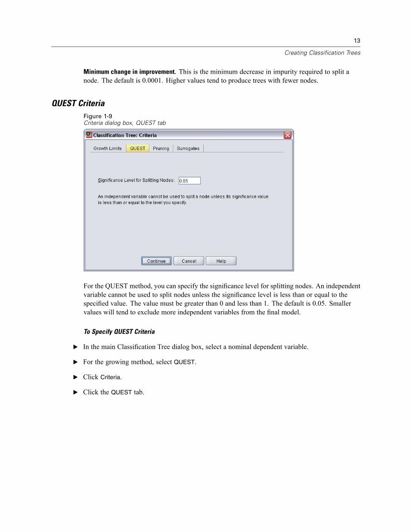
Return on investment (ROI). Line chart of cumulative ROI (return on investment). ROI is computedas the ratio of profits to expenses. Available only for categorical dependent variables withdefined profits.
The ROI chart plots the same values that you would see in the ROI column in the gain summaryfor percentiles table.
34
Chapter 1
Figure 1-30Gain summary for percentiles table and ROI chart
Percentile increment. For all percentile charts, this setting controls the percentile incrementsdisplayed on the chart: 1, 2, 5, 10, 20, or 25.
35
Creating Classification Trees
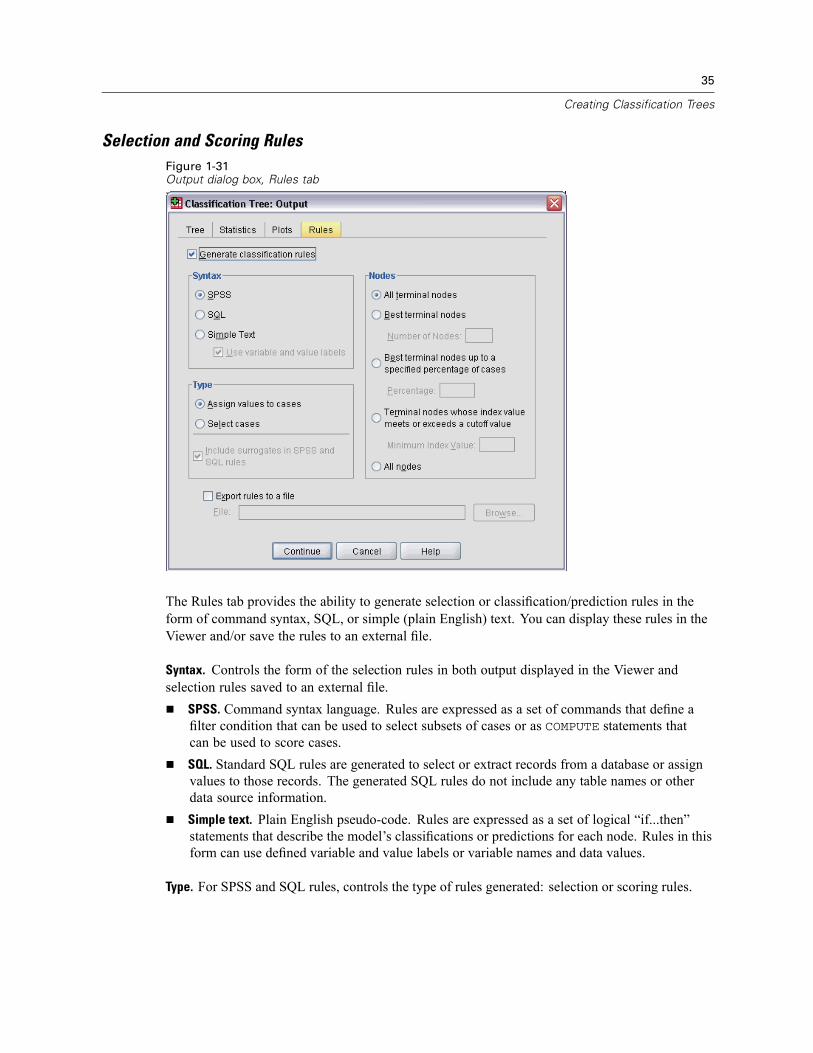
Selection and Scoring RulesFigure 1-31Output dialog box, Rules tab
The Rules tab provides the ability to generate selection or classification/prediction rules in theform of command syntax, SQL, or simple (plain English) text. You can display these rules in theViewer and/or save the rules to an external file.
Syntax. Controls the form of the selection rules in both output displayed in the Viewer andselection rules saved to an external file.
SPSS. Command syntax language. Rules are expressed as a set of commands that define afilter condition that can be used to select subsets of cases or as COMPUTE statements thatcan be used to score cases.SQL. Standard SQL rules are generated to select or extract records from a database or assignvalues to those records. The generated SQL rules do not include any table names or otherdata source information.Simple text. Plain English pseudo-code. Rules are expressed as a set of logical “if...then”statements that describe the model’s classifications or predictions for each node. Rules in thisform can use defined variable and value labels or variable names and data values.
Type. For SPSS and SQL rules, controls the type of rules generated: selection or scoring rules.

36
Chapter 1
Assign values to cases. The rules can be used to assign the model’s predictions to cases thatmeet node membership criteria. A separate rule is generated for each node that meets thenode membership criteria.Select cases. The rules can be used to select cases that meet node membership criteria. ForSPSS and SQL rules, a single rule is generated to select all cases that meet the selectioncriteria.
Include surrogates in SPSS and SQL rules. For CRT and QUEST, you can include surrogatepredictors from the model in the rules. Rules that include surrogates can be quite complex. Ingeneral, if you just want to derive conceptual information about your tree, exclude surrogates. Ifsome cases have incomplete independent variable (predictor) data and you want rules that mimicyour tree, include surrogates. For more information, see Surrogates on p. 15.
Nodes. Controls the scope of the generated rules. A separate rule is generated for each nodeincluded in the scope.
All terminal nodes. Generates rules for each terminal node.Best terminal nodes. Generates rules for the top n terminal nodes based on index values. Ifthe number exceeds the number of terminal nodes in the tree, rules are generated for allterminal nodes. (See note below.)Best terminal nodes up to a specified percentage of cases. Generates rules for terminal nodesfor the top n percentage of cases based on index values. (See note below.)Terminal nodes whose index value meets or exceeds a cutoff value. Generates rules for allterminal nodes with an index value greater than or equal to the specified value. An indexvalue greater than 100 means that the percentage of cases in the target category in that nodeexceeds the percentage in the root node. (See note below.)All nodes. Generates rules for all nodes.
Note 1: Node selection based on index values is available only for categorical dependent variableswith defined target categories. If you have specified multiple target categories, a separate setof rules is generated for each target category.
Note 2: For SPSS and SQL rules for selecting cases (not rules for assigning values), All nodes andAll terminal nodes will effectively generate a rule that selects all cases used in the analysis.
Export rules to a file. Saves the rules in an external text file.
You can also generate and save selection or scoring rules interactively, based on selected nodes inthe final tree model. For more information, see Case Selection and Scoring Rules in Chapter 2on p. 44.
Note: If you apply rules in the form of command syntax to another data file, that data file mustcontain variables with the same names as the independent variables included in the final model,measured in the same metric, with the same user-defined missing values (if any).

Chapter
2Tree Editor
With the Tree Editor, you can:Hide and show selected tree branches.Control display of node content, statistics displayed at node splits, and other information.Change node, background, border, chart, and font colors.Change font style and size.Change tree alignment.Select subsets of cases for further analysis based on selected nodes.Create and save rules for selecting or scoring cases based on selected nodes.
To edit a tree model:
E Double-click the tree model in the Viewer window.
or
E Right-click the tree model in the Viewer window, and from the context menu choose:SPSS Tree Object
Open
Hiding and Showing Nodes
To hide (collapse) all the child nodes in a branch beneath a parent node:
E Click the minus sign (–) in the small box below the lower right corner of the parent node.
All nodes beneath the parent node on that branch will be hidden.
To show (expand) the child nodes in a branch beneath a parent node:
E Click the plus sign (+) in the small box below the lower right corner of the parent node.
Note: Hiding the child nodes on a branch is not the same as pruning a tree. If you want a prunedtree, you must request pruning before you create the tree, and pruned branches are not included inthe final tree. For more information, see Pruning Trees in Chapter 1 on p. 14.
37

38
Chapter 2
Figure 2-1Expanded and collapsed tree
Selecting Multiple Nodes
You can select cases, generate scoring and selections rules, and perform other actions based on thecurrently selected node(s). To select multiple nodes:
E Click a node you want to select.
E Ctrl-click the other nodes you want to select.
You can multiple-select sibling nodes and/or parent nodes in one branch and child nodes in anotherbranch. You cannot, however, use multiple selection on a parent node and a child/descendantof the same node branch.
Working with Large Trees
Tree models may sometimes contain so many nodes and branches that it is difficult or impossibleto view the entire tree at full size. There are a number of features that you may find useful whenworking with large trees:
Tree map. You can use the tree map, a much smaller, simplified version of the tree, to navigatethe tree and select nodes. For more information, see Tree Map on p. 39.Scaling. You can zoom out and zoom in by changing the scale percentage for the tree display.For more information, see Scaling the Tree Display on p. 39.Node and branch display. You can make a tree more compact by displaying only tablesor only charts in the nodes and/or suppressing the display of node labels or independentvariable information. For more information, see Controlling Information Displayed in theTree on p. 41.

39
Tree Editor
Tree Map
The tree map provides a compact, simplified view of the tree that you can use to navigate thetree and select nodes.
To use the tree map window:
E From the Tree Editor menus choose:View
Tree Map
Figure 2-2Tree map window
The currently selected node is highlighted in both the Tree Model Editor and the tree mapwindow.The portion of the tree that is currently in the Tree Model Editor view area is indicated witha red rectangle in the tree map. Right-click and drag the rectangle to change the section ofthe tree displayed in the view area.If you select a node in the tree map that isn’t currently in the Tree Editor view area, the viewshifts to include the selected node.Multiple node selection works the same in the tree map as in the Tree Editor: Ctrl-clickto select multiple nodes. You cannot use multiple selection on a parent node and achild/descendant of the same node branch.
Scaling the Tree Display
By default, trees are automatically scaled to fit in the Viewer window, which can result in sometrees that are initially very difficult to read. You can select a preset scale setting or enter your owncustom scale value of between 5% and 200%.

40
Chapter 2
To change the scale of the tree:
E Select a scale percentage from the drop-down list on the toolbar, or enter a custom percentagevalue.
or
E From the Tree Editor menus choose:View
Scale...
Figure 2-3Scale dialog box
You can also specify a scale value before you create the tree model. For more information, seeOutput in Chapter 1 on p. 23.
Node Summary Window
The node summary window provides a larger view of the selected nodes. You can also use thesummary window to view, apply, or save selection or scoring rules based on the selected nodes.
Use the View menu in the node summary window to switch between views of a summarytable, chart, or rules.Use the Rules menu in the node summary window to select the type of rules you want to see.For more information, see Case Selection and Scoring Rules on p. 44.All views in the node summary window reflect a combined summary for all selected nodes.
To use the node summary window:
E Select the nodes in the Tree Editor. To select multiple nodes, use Ctrl-click.
E From the menus choose:View
Summary

41
Tree Editor
Figure 2-4Tree with charts in nodes and table for selected node in summary window
Controlling Information Displayed in the Tree
The Options menu in the Tree Editor allows you to control the display of node contents,independent variable (predictor) names and statistics, node definitions, and other settings. Manyof these settings can be also be controlled from the toolbar.
Setting Options Menu SelectionHighlight predicted category (categorical dependentvariable)
Highlight Predicted
Tables and/or charts in node Node ContentsSignificance test values and p values Independent Variable StatisticsIndependent (predictor) variable names Independent VariablesIndependent (predictor) value(s) for nodes Node DefinitionsAlignment (top-down, left-right, right-left) OrientationChart legend Legend

42
Chapter 2
Figure 2-5Tree elements
Changing Tree Colors and Text FontsYou can change the following colors in the tree:
Node border, background, and text colorBranch color and branch text colorTree background colorPredicted category highlight color (categorical dependent variables)Node chart colors
You can also change the type font, style, and size for all text in the tree.
Note: You cannot change color or font attributes for individual nodes or branches. Color changesapply to all elements of the same type, and font changes (other than color) apply to all chartelements.
To change colors and text font attributes:
E Use the toolbar to change font attributes for the entire tree or colors for different tree elements.(ToolTips describe each control on the toolbar when you put the mouse cursor on the control.)
or
E Double-click anywhere in the Tree Editor to open the Properties window, or from the menuschoose:View
Properties
E For border, branch, node background, predicted category, and tree background, click the Color tab.
E For font colors and attributes, click the Text tab.
E For node chart colors, click the Node Charts tab.

43
Tree Editor
Figure 2-6Properties window, Color tab
Figure 2-7Properties window, Text tab

44
Chapter 2
Figure 2-8Properties window, Node Charts tab
Case Selection and Scoring Rules
You can use the Tree Editor to:Select subsets of cases based on the selected node(s). For more information, see FilteringCases on p. 44.Generate case selection rules or scoring rules in SPSS or SQL format. For more information,see Saving Selection and Scoring Rules on p. 45.
You can also automatically save rules based on various criteria when you run the ClassificationTree procedure to create the tree model. For more information, see Selection and Scoring Rules inChapter 1 on p. 35.
Filtering Cases
If you want to know more about the cases in a particular node or group of nodes, you can select asubset of cases for further analysis based on the selected nodes.
E Select the nodes in the Tree Editor. To select multiple nodes, use Ctrl-click.
E From the menus choose:Rules
Filter Cases...
E Enter a filter variable name. Cases from the selected nodes will receive a value of 1 for thisvariable. All other cases will receive a value of 0 and will be excluded from subsequent analysisuntil you change the filter status.
E Click OK.

45
Tree Editor
Figure 2-9Filter Cases dialog box
Saving Selection and Scoring Rules
You can save case selection or scoring rules in an external file and then apply those rules to adifferent data source. The rules are based on the selected nodes in the Tree Editor.
Syntax. Controls the form of the selection rules in both output displayed in the Viewer andselection rules saved to an external file.
SPSS. Command syntax language. Rules are expressed as a set of commands that define afilter condition that can be used to select subsets of cases or as COMPUTE statements thatcan be used to score cases.SQL. Standard SQL rules are generated to select/extract records from a database or assignvalues to those records. The generated SQL rules do not include any table names or otherdata source information.
Type. You can create selection or scoring rules.Select cases. The rules can be used to select cases that meet node membership criteria. ForSPSS and SQL rules, a single rule is generated to select all cases that meet the selectioncriteria.Assign values to cases. The rules can be used to assign the model’s predictions to cases thatmeet node membership criteria. A separate rule is generated for each node that meets thenode membership criteria.
Include surrogates. For CRT and QUEST, you can include surrogate predictors from the modelin the rules. Rules that include surrogates can be quite complex. In general, if you just want toderive conceptual information about your tree, exclude surrogates. If some cases have incompleteindependent variable (predictor) data and you want rules that mimic your tree, include surrogates.For more information, see Surrogates in Chapter 1 on p. 15.
To save case selection or scoring rules:
E Select the nodes in the Tree Editor. To select multiple nodes, use Ctrl-click.
E From the menus choose:Rules
Export...
E Select the type of rules you want and enter a filename.

46
Chapter 2
Figure 2-10Export Rules dialog box
Note: If you apply rules in the form of command syntax to another data file, that data file mustcontain variables with the same names as the independent variables included in the final model,measured in the same metric, with the same user-defined missing values (if any).

Chapter
3Data Assumptions and Requirements
The Classification Tree procedure assumes that:The appropriate measurement level has been assigned to all analysis variables.For categorical (nominal, ordinal) dependent variables, value labels have been defined for allcategories that should be included in the analysis.
We’ll use the file tree_textdata.sav to illustrate the importance of both of these requirements. Thisdata file reflects the default state of data read or entered before defining any attributes, suchas measurement level or value labels. For more information, see Sample Files in Appendix Aon p. 97.
Effects of Measurement Level on Tree Models
Both variables in this data file are numeric. By default, numeric variables are assumed to have ascale measurement level. But (as we will see later) both variables are really categorical variablesthat rely on numeric codes to stand for category values.
E To run a Classification Tree analysis, from the menus choose:Analyze
ClassifyTree...
47

48
Chapter 3
The icons next to the two variables in the source variable list indicate that they will be treated asscale variables.
Figure 3-1Classification Tree main dialog box with two scale variables
E Select dependent as the dependent variable.
E Select independent as the independent variable.
E Click OK to run the procedure.
E Open the Classification Tree dialog box again and click Reset.
E Right-click dependent in the source list and select Nominal from the context menu.
E Do the same for the variable independent in the source list.

49
Data Assumptions and Requirements
Now the icons next to each variable indicate that they will be treated as nominal variables.
Figure 3-2Nominal icons in source list
E Select dependent as the dependent variable and independent as the independent variable, andclick OK to run the procedure again.
Now let’s compare the two trees. First, we’ll look at the tree in which both numeric variables aretreated as scale variables.
Figure 3-3Tree with both variables treated as scale

50
Chapter 3
Each node of tree shows the “predicted” value, which is the mean value for the dependentvariable at that node. For a variable that is actually categorical, the mean may not be ameaningful statistic.The tree has four child nodes, one for each value of the independent variable.
Tree models will often merge similar nodes, but for a scale variable, only contiguous values canbe merged. In this example, no contiguous values were considered similar enough to mergeany nodes together.The tree in which both variables are treated as nominal is somewhat different in several respects.
Figure 3-4Tree with both variables treated as nominal
Instead of a predicted value, each node contains a frequency table that shows the number ofcases (count and percentage) for each category of the dependent variable.The “predicted” category—the category with the highest count in each node—is highlighted.For example, the predicted category for node 2 is category 3.Instead of four child nodes, there are only three, with two values of the independent variablemerged into a single node.
The two independent values merged into the same node are 1 and 4. Since, by definition, there isno inherent order to nominal values, merging of noncontiguous values is allowed.
Permanently Assigning Measurement Level
When you change the measurement level for a variable in the Classification Tree dialog box, thechange is only temporary; it is not saved with the data file. Furthermore, you may not alwaysknow what the correct measurement level should be for all variables.

51
Data Assumptions and Requirements
Define Variable Properties can help you determine the correct measurement level for eachvariable and permanently change the assigned measurement level. To use Define VariableProperties:
E From the menus choose:Data
Define Variable Properties...
Effects of Value Labels on Tree Models
The Classification Tree dialog box interface assumes that either all nonmissing values of acategorical (nominal, ordinal) dependent variable have defined value labels or none of them do.Some features are not available unless at least two nonmissing values of the categorical dependentvariable have value labels. If at least two nonmissing values have defined value labels, any caseswith other values that do not have value labels will be excluded from the analysis.The original data file in this example contains no defined value labels, and when the dependent
variable is treated as nominal, the tree model uses all nonmissing values in the analysis. In thisexample, those values are 1, 2, and 3.But what happens when we define value labels for some, but not all, values of the dependent
variable?
E In the Data Editor window, click the Variable View tab.
E Click the Values cell for the variable dependent.
Figure 3-5Defining value labels for dependent variable
E First, enter 1 for Value and Yes for Value Label, and then click Add.
E Next, enter 2 for Value and No for Value Label, and then click Add again.
E Then click OK.

52
Chapter 3
E Open the Classification Tree dialog box again. The dialog box should still have dependent selectedas the dependent variable, with a nominal measurement level.
E Click OK to run the procedure again.
Figure 3-6Tree for nominal dependent variable with partial value labels
Now only the two dependent variable values with defined value labels are included in the treemodel. All cases with a value of 3 for the dependent variable have been excluded, which mightnot be readily apparent if you aren’t familiar with the data.
Assigning Value Labels to All Values
To avoid accidental omission of valid categorical values from the analysis, use Define VariableProperties to assign value labels to all dependent variable values found in the data.

53
Data Assumptions and Requirements
When the data dictionary information for the variable name is displayed in the Define VariableProperties dialog box, you can see that although there are over 300 cases with a value of 3 for thatvariable, no value label has been defined for that value.
Figure 3-7Variable with partial value labels in Define Variable Properties dialog box

Chapter
4Using Classification Trees to EvaluateCredit Risk
A bank maintains a database of historic information on customers who have taken out loans fromthe bank, including whether or not they repaid the loans or defaulted. Using classification trees,you can analyze the characteristics of the two groups of customers and build models to predictthe likelihood that loan applicants will default on their loans.The credit data are stored in tree_credit.sav. For more information, see Sample Files in
Appendix A on p. 97.
Creating the Model
The Classification Tree Procedure offers several different methods for creating tree models. Forthis example, we’ll use the default method:
CHAID. Chi-squared Automatic Interaction Detection. At each step, CHAID chooses theindependent (predictor) variable that has the strongest interaction with the dependent variable.Categories of each predictor are merged if they are not significantly different with respect to thedependent variable.
Building the CHAID Tree Model
E To run a Classification Tree analysis, from the menus choose:Analyze
ClassifyTree...
54

55
Using Classification Trees to Evaluate Credit Risk
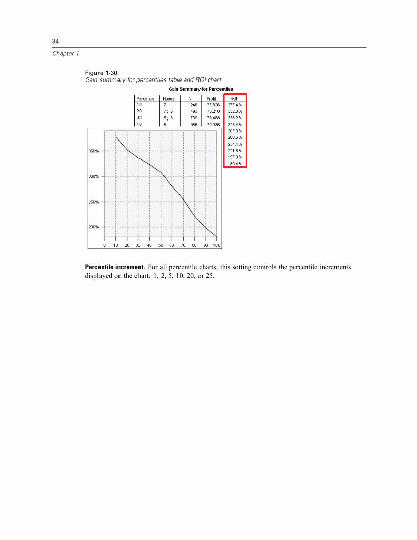
Figure 4-1Classification Tree dialog box
E Select Credit rating as the dependent variable.
E Select all the remaining variables as independent variables. (The procedure will automaticallyexclude any variables that don’t make a significant contribution to the final model.)
At this point, you could run the procedure and produce a basic tree model, but we’re going toselect some additional output and make a few minor adjustments to the criteria used to generatethe model.
Selecting Target Categories
E Click the Categories button right below the selected dependent variable.

56
Chapter 4
This opens the Categories dialog box, where you can specify the dependent variable targetcategories of interest. Target categories do not affect the tree model itself, but some output andoptions are available only if you have selected target categories.
Figure 4-2Categories dialog box
E Select (check) the Target check box for the Bad category. Customers with a bad credit rating(defaulted on a loan) will be treated as the target category of interest.
E Click Continue.
Specifying Tree Growing Criteria
For this example, we want to keep the tree fairly simple, so we’ll limit the tree growth by raisingthe minimum number of cases for parent and child nodes.
E In the main Classification Tree dialog box, click Criteria.

57
Using Classification Trees to Evaluate Credit Risk
Figure 4-3Criteria dialog box, Growth Limits tab
E In the Minimum Number of Cases group, type 400 for Parent Node and 200 for Child Node.
E Click Continue.
Selecting Additional Output
E In the main Classification Tree dialog box, click Output.

58
Chapter 4
This opens a tabbed dialog box, where you can select various types of additional output.
Figure 4-4Output dialog box, Tree tab
E On the Tree tab, select (check) Tree in table format.
E Then click the Plots tab.

59
Using Classification Trees to Evaluate Credit Risk
Figure 4-5Output dialog box, Plots tab
E Select (check) Gain and Index.
Note: These charts require a target category for the dependent variable. In this example, the Plotstab isn’t accessible until after you have specified one or more target categories.
E Click Continue.
Saving Predicted Values
You can save variables that contain information about model predictions. For example, you cansave the credit rating predicted for each case and then compare those predictions to the actualcredit ratings.
E In the main Classification Tree dialog box, click Save.

60
Chapter 4
Figure 4-6Save dialog box
E Select (check) Terminal node number, Predicted value, and Predicted probabilities.
E Click Continue.
E In the main Classification Tree dialog box, click OK to run the procedure.
Evaluating the Model
For this example, the model results include:Tables that provide information about the model.Tree diagram.Charts that provide an indication of model performance.Model prediction variables added to the active dataset.

61
Using Classification Trees to Evaluate Credit Risk
Model Summary TableFigure 4-7Model summary
The model summary table provides some very broad information about the specifications usedto build the model and the resulting model.
The Specifications section provides information on the settings used to generate the treemodel, including the variables used in the analysis.The Results section displays information on the number of total and terminal nodes, depthof the tree (number of levels below the root node), and independent variables includedin the final model.
Five independent variables were specified, but only three were included in the final model. Thevariables for education and number of current car loans did not make a significant contribution tothe model, so they were automatically dropped from the final model.

62
Chapter 4
Tree DiagramFigure 4-8Tree diagram for credit rating model
The tree diagram is a graphic representation of the tree model. This tree diagram shows that:Using the CHAID method, income level is the best predictor of credit rating.For the low income category, income level is the only significant predictor of credit rating. Ofthe bank customers in this category, 82% have defaulted on loans. Since there are no childnodes below it, this is considered a terminal node.For the medium and high income categories, the next best predictor is number of credit cards.For medium income customers with five or more credit cards, the model includes one morepredictor: age. Over 80% of those customers 28 or younger have a bad credit rating, whileslightly less than half of those over 28 have a bad credit rating.
You can use the Tree Editor to hide and show selected branches, change colors and fonts, andselect subsets of cases based on selected nodes. For more information, see Selecting Cases inNodes on p. 68.

63
Using Classification Trees to Evaluate Credit Risk
Tree TableFigure 4-9Tree table for credit rating
The tree table, as the name suggests, provides most of the essential tree diagram information in theform of a table. For each node, the table displays:
The number and percentage of cases in each category of the dependent variable.The predicted category for the dependent variable. In this example, the predicted categoryis the credit rating category with more than 50% of cases in that node, since there are onlytwo possible credit ratings.The parent node for each node in the tree. Note that node 1—the low income level node—isnot the parent node of any node. Since it is a terminal node, it has no child nodes.
Figure 4-10Tree table for credit rating (continued)
The independent variable used to split the node.The chi-square value (since the tree was generated with the CHAID method), degrees offreedom (df), and significance level (Sig.) for the split. For most practical purposes, youwill probably be interested only in the significance level, which is less than 0.0001 for allsplits in this model.The value(s) of the independent variable for that node.
Note: For ordinal and scale independent variables, you may see ranges in the tree and tree tableexpressed in the general form (value1, value2], which basically means “greater than value1 andless than or equal to value2.” In this example, income level has only three possible values—Low,

64
Chapter 4
Medium, and High—and (Low, Medium] simply means Medium. In a similar fashion, >Mediummeans High.
Gains for Nodes
Figure 4-11Gains for nodes
The gains for nodes table provides a summary of information about the terminal nodes in themodel.
Only the terminal nodes—nodes at which the tree stops growing—are listed in this table.Frequently, you will be interested only in the terminal nodes, since they represent the bestclassification predictions for the model.Since gain values provide information about target categories, this table is available only ifyou specified one or more target categories. In this example, there is only one target category,so there is only one gains for nodes table.Node N is the number of cases in each terminal node, and Node Percent is the percentageof the total number of cases in each node.Gain N is the number of cases in each terminal node in the target category, and Gain Percent isthe percentage of cases in the target category with respect to the overall number of cases in thetarget category—in this example, the number and percentage of cases with a bad credit rating.For categorical dependent variables, Response is the percentage of cases in the node in thespecified target category. In this example, these are the same percentages displayed for theBad category in the tree diagram.For categorical dependent variables, Index is the ratio of the response percentage for the targetcategory compared to the response percentage for the entire sample.
Index Values
The index value is basically an indication of how far the observed target category percentagefor that node differs from the expected percentage for the target category. The target categorypercentage in the root node represents the expected percentage before the effects of any of theindependent variables are considered.
An index value of greater than 100% means that there are more cases in the target category thanthe overall percentage in the target category. Conversely, an index value of less than 100% meansthere are fewer cases in the target category than the overall percentage.

65
Using Classification Trees to Evaluate Credit Risk
Gains ChartFigure 4-12Gains chart for bad credit rating target category
This gains chart indicates that the model is a fairly good one.
Cumulative gains charts always start at 0% and end at 100% as you go from one end to the other.For a good model, the gains chart will rise steeply toward 100% and then level off. A model thatprovides no information will follow the diagonal reference line.
Index ChartFigure 4-13Index chart for bad credit rating target category
The index chart also indicates that the model is a good one. Cumulative index charts tend to startabove 100% and gradually descend until they reach 100%.

66
Chapter 4
For a good model, the index value should start well above 100%, remain on a high plateau as youmove along, and then trail off sharply toward 100%. For a model that provides no information, theline will hover around 100% for the entire chart.
Risk Estimate and ClassificationFigure 4-14Risk and classification tables
The risk and classification tables provide a quick evaluation of how well the model works.The risk estimate of 0.205 indicates that the category predicted by the model (good or badcredit rating) is wrong for 20.5% of the cases. So the “risk” of misclassifying a customer isapproximately 21%.The results in the classification table are consistent with the risk estimate. The table showsthat the model classifies approximately 79.5% of the customers correctly.
The classification table does, however, reveal one potential problem with this model: for thosecustomers with a bad credit rating, it predicts a bad rating for only 65% of them, which means that35% of customers with a bad credit rating are inaccurately classified with the “good” customers.

67
Using Classification Trees to Evaluate Credit Risk
Predicted ValuesFigure 4-15New variables for predicted values and probabilities
Four new variables have been created in the active dataset:
NodeID. The terminal node number for each case.
PredictedValue. The predicted value of the dependent variable for each case. Since the dependentvariable is coded 0 = Bad and 1 = Good, a predicted value of 0 means that the case is predictedto have a bad credit rating.
PredictedProbability. The probability that the case belongs in each category of the dependentvariable. Since there are only two possible values for the dependent variable, two variablesare created:
PredictedProbability_1. The probability that the case belongs in the bad credit rating category.PredictedProbability_2. The probability that the case belongs in the good credit rating category.
The predicted probability is simply the proportion of cases in each category of the dependentvariable for the terminal node that contains each case. For example, in node 1, 82% of the casesare in the bad category and 18% are in the good category, resulting in predicted probabilities of0.82 and 0.18, respectively.
For a categorical dependent variable, the predicted value is the category with the highestproportion of cases in the terminal node for each case. For example, for the first case, the predictedvalue is 1 (good credit rating), since approximately 56% of the cases in its terminal node have agood credit rating. Conversely, for the second case, the predicted value is 0 (bad credit rating),since approximately 81% of cases in its terminal node have a bad credit rating.
If you have defined costs, however, the relationship between predicted category and predictedprobabilities may not be quite so straightforward. For more information, see Assigning Costs toOutcomes on p. 72.

68
Chapter 4
Refining the Model
Overall, the model has a correct classification rate of just under 80%. This is reflected in mostof the terminal nodes, where the predicted category—the highlighted category in the node—isthe same as the actual category for 80% or more of the cases.There is, however, one terminal node where cases are fairly evenly split between good and
bad credit ratings. In node 9, the predicted credit rating is “good,” but only 56% of the cases inthat node actually have a good credit rating. That means that almost half of the cases in that node(44%) will have the wrong predicted category. And if the primary concern is identifying badcredit risks, this node doesn’t perform very well.
Selecting Cases in Nodes
Let’s look at the cases in node 9 to see if the data reveal any useful additional information.
E Double-click the tree in the Viewer to open the Tree Editor.
E Click node 9 to select it. (If you want to select multiple nodes, use Ctrl-click).
E From the Tree Editor menus choose:Rules
Filter Cases...
Figure 4-16Filter Cases dialog box
The Filter Cases dialog box will create a filter variable and apply a filter setting based on thevalues of that variable. The default filter variable name is filter_$.
Cases from the selected nodes will receive a value of 1 for the filter variable.All other cases will receive a value of 0 and will be excluded from subsequent analysesuntil you change the filter status.
In this example, that means cases that aren’t in node 9 will be filtered out (but not deleted) for now.
E Click OK to create the filter variable and apply the filter condition.

69
Using Classification Trees to Evaluate Credit Risk
Figure 4-17Filtered cases in Data Editor
In the Data Editor, cases that have been filtered out are indicated with a diagonal slash throughthe row number. Cases that are not in node 9 are filtered out. Cases in node 9 are not filtered;so subsequent analyses will include only cases from node 9.
Examining the Selected Cases
As a first step in examining the cases in node 9, you might want to look at the variables not used inthe model. In this example, all variables in the data file were included in the analysis, but twoof them were not included in the final model: education and car loans. Since there’s probably agood reason why the procedure omitted them from the final model, they probably won’t tell usmuch, but let’s take a look anyway.
E From the menus choose:Analyze
Descriptive StatisticsCrosstabs...

70
Chapter 4
Figure 4-18Crosstabs dialog box
E Select Credit rating for the row variable.
E Select Education and Car loans for the column variables.
E Click Cells.

71
Using Classification Trees to Evaluate Credit Risk
Figure 4-19Crosstabs Cell Display dialog box
E In the Percentages group, select (check) Row.
E Then click Continue, and in the main Crosstabs dialog box, click OK to run the procedure.
Examining the crosstabulations, you can see that for the two variables not included in the model,there isn’t a great deal of difference between cases in the good and bad credit rating categories.
Figure 4-20Crosstabulations for cases in selected node
For education, slightly more than half of the cases with a bad credit rating have only a highschool education, while slightly more than half with a good credit rating have a collegeeducation—but this difference is not statistically significant.

72
Chapter 4
For car loans, the percentage of good credit cases with only one or no car loans is higher thanthe corresponding percentage for bad credit cases, but the vast majority of cases in bothgroups has two or more car loans.
So, although you now get some idea of why these variables were not included in the final model,you unfortunately haven’t gained any insight into how to get better prediction for node 9. Ifthere were other variables not specified for the analysis, you might want to examine some ofthem before proceeding.
Assigning Costs to Outcomes
As noted earlier, aside from the fact that almost half of the cases in node 9 fall in each creditrating category, the fact that the predicted category is “good” is problematic if your mainobjective is to build a model that correctly identifies bad credit risks. Although you may not beable to improve the performance of node 9, you can still refine the model to improve the rate ofcorrect classification for bad credit rating cases—although this will also result in a higher rate ofmisclassification for good credit rating cases.
First, you need to turn off case filtering so that all cases will be used in the analysis again.
E From the menus choose:Data
Select Cases...

73
Using Classification Trees to Evaluate Credit Risk
E In the Select Cases dialog box, select All cases, and then click OK.
Figure 4-21Select Cases dialog box
E Open the Classification Tree dialog box again, and click Options.

74
Chapter 4
E Click the Misclassification Costs tab.
Figure 4-22Options dialog box, Misclassification Costs tab
E Select Custom, and for Bad Actual Category / Good Predicted Category, enter a value of 2.
This tells the procedure that the “cost” of incorrectly classifying a bad credit risk as good is twiceas high as the “cost” of incorrectly classifying a good credit risk as bad.
E Click Continue, and then in the main dialog box, click OK to run the procedure.

75
Using Classification Trees to Evaluate Credit Risk
Figure 4-23Tree model with adjusted cost values
At first glance, the tree generated by the procedure looks essentially the same as the original tree.Closer inspection, however, reveals that although the distribution of cases in each node hasn’tchanged, some predicted categories have changed.For the terminal nodes, the predicted category remains the same in all nodes except one:
node 9. The predicted category is now Bad even though slightly more than half of the casesare in the Good category.Since we told the procedure that there was a higher cost for misclassifying bad credit risks as
good, any node where the cases are fairly evenly distributed between the two categories now has apredicted category of Bad even if a slight majority of cases is in the Good category.

76
Chapter 4
This change in predicted category is reflected in the classification table.
Figure 4-24Risk and classification tables based on adjusted costs
Almost 86% of the bad credit risks are now correctly classified, compared to only 65% before.On the other hand, correct classification of good credit risks has decreased from 90% to 71%,and overall correct classification has decreased from 79.5% to 77.1%.
Note also that the risk estimate and the overall correct classification rate are no longer consistentwith each other. You would expect a risk estimate of 0.229 if the overall correct classification rateis 77.1%. Increasing the cost of misclassification for bad credit cases has, in this example, inflatedthe risk value, making its interpretation less straightforward.
Summary
You can use tree models to classify cases into groups identified by certain characteristics, such asthe characteristics associated with bank customers with good and bad credit records. If a particularpredicted outcome is more important than other possible outcomes, you can refine the model toassociate a higher misclassification cost for that outcome—but reducing misclassification rates forone outcome will increase misclassification rates for other outcomes.

Chapter
5Building a Scoring Model
One of the most powerful and useful features of the Classification Tree procedure is the ability tobuild models that can then be applied to other data files to predict outcomes. For example, basedon a data file that contains both demographic information and information on vehicle purchaseprice, we can build a model that can be used to predict how much people with similar demographiccharacteristics are likely to spend on a new car—and then apply that model to other data fileswhere demographic information is available but information on previous vehicle purchasing is not.For this example, we’ll use the data file tree_car.sav. For more information, see Sample Files in
Appendix A on p. 97.
Building the ModelE To run a Classification Tree analysis, from the menus choose:
AnalyzeClassify
Tree...
77

78
Chapter 5
Figure 5-1Classification Tree dialog box
E Select Price of primary vehicle as the dependent variable.
E Select all the remaining variables as independent variables. (The procedure will automaticallyexclude any variables that don’t make a significant contribution to the final model.)
E For the growing method, select CRT.
E Click Output.

79
Building a Scoring Model
Figure 5-2Output dialog box, Rules tab
E Click the Rules tab.
E Select (check) Generate classification rules.
E For Syntax, select SPSS.
E For Type, select Assign values to cases.
E Select (check) Export rules to a file and enter a filename and directory location.
Remember the filename and location or write it down because you’ll need it a little later. If youdon’t include a directory path, you may not know where the file has been saved. You can use theBrowse button to navigate to a specific (and valid) directory location.
E Click Continue, and then click OK to run the procedure and build the tree model.

80
Chapter 5
Evaluating the Model
Before applying the model to other data files, you probably want to make sure that the modelworks reasonably well with the original data used to build it.
Model SummaryFigure 5-3Model summary table
The model summary table indicates that only three of the selected independent variables made asignificant enough contribution to be included in the final model: income, age, and education.This is important information to know if you want to apply this model to other data files, sincethe independent variables used in the model must be present in any data file to which you wantto apply the model.The summary table also indicates that the tree model itself is probably not a particularly simple
one since it has 29 nodes and 15 terminal nodes. This may not be an issue if you want a reliablemodel that can be applied in a practical fashion rather than a simple model that is easy to describeor explain. Of course, for practical purposes, you probably also want a model that doesn’t rely ontoo many independent (predictor) variables. In this case, that’s not a problem since only threeindependent variables are included in the final model.

81
Building a Scoring Model
Tree Model Diagram
Figure 5-4Tree model diagram in Tree Editor
The tree model diagram has so many nodes that it may be difficult to see the whole model atonce at a size where you can still read the node content information. You can use the tree mapto see the entire tree:
E Double-click the tree in the Viewer to open the Tree Editor.
E From the Tree Editor menus choose:View
Tree Map

82
Chapter 5
Figure 5-5Tree map
The tree map shows the entire tree. You can change the size of the tree map window, and itwill grow or shrink the map display of the tree to fit the window size.The highlighted area in the tree map is the area of the tree currently displayed in the TreeEditor.You can use the tree map to navigate the tree and select nodes.
For more information, see Tree Map in Chapter 2 on p. 39.
For scale dependent variables, each node shows the mean and standard deviation of the dependentvariable. Node 0 displays an overall mean vehicle purchase price of about 29.9 (in thousands),with a standard deviation of about 21.6.
Node 1, which represents cases with an income of less than 75 (also in thousands) has amean vehicle price of only 18.7.In contrast, node 2, which represents cases with an income of 75 or more, has a mean vehicleprice of 60.9.
Further investigation of the tree would show that age and education also display a relationshipwith vehicle purchase price, but right now we’re primarily interested in the practical application ofthe model rather than a detailed examination of its components.
Risk EstimateFigure 5-6Risk table
None of the results we’ve examined so far tell us if this is a particularly good model. Oneindicator of the model’s performance is the risk estimate. For a scale dependent variable, the riskestimate is a measure of the within-node variance, which by itself may not tell you a great deal. Alower variance indicates a better model, but the variance is relative to the unit of measurement.

83
Building a Scoring Model
If, for example, price was recorded in ones instead of thousands, the risk estimate would be athousand times larger.
To provide a meaningful interpretation for the risk estimate with a scale dependent variablerequires a little work:
Total variance equals the within-node (error) variance plus the between-node (explained)variance.The within-node variance is the risk estimate value: 68.485.The total variance is the variance for the dependent variables before consideration of anyindependent variables, which is the variance at the root node.The standard deviation displayed at the root node is 21.576; so the total variance is thatvalue squared: 465.524.The proportion of variance due to error (unexplained variance) is 68.485 / 465.524 = 0.147.The proportion of variance explained by the model is 1 – 0.147 = 0.853, or 85.3%, whichindicates that this is a fairly good model. (This has a similar interpretation to the overallcorrect classification rate for a categorical dependent variable.)
Applying the Model to Another Data File
Having determined that the model is reasonably good, we can now apply that model to other datafiles containing similar age, income, and education variables and generate a new variable thatrepresents the predicted vehicle purchase price for each case in that file. This process is oftenreferred to as scoring.When we generated the model, we specified that “rules” for assigning values to cases should
be saved in a text file—in the form of command syntax. We will now use the commands inthat file to generate scores in another data file.
E Open the data file tree_score_car.sav. For more information, see Sample Files in Appendix Aon p. 97.
E Next, from the menus choose:File
NewSyntax
E In the command syntax window, type:
INSERT FILE='/temp/car_scores.sps'.

84
Chapter 5
If you used a different filename or location, make the appropriate changes.
Figure 5-7Syntax window with INSERT command to run a command file
The INSERT command will run the commands in the specified file, which is the “rules” file thatwas generated when we created the model.
E From the command syntax window menus choose:Run
All
Figure 5-8Predicted values added to data file
This adds two new variables to the data file:nod_001 contains the terminal node number predicted by the model for each case.pre_001 contains the predicted value for vehicle purchase price for each case.
Since we requested rules for assigning values for terminal nodes, the number of possible predictedvalues is the same as the number of terminal nodes, which in this case is 15. For example, everycase with a predicted node number of 10 will have the same predicted vehicle purchase price:

85
Building a Scoring Model
30.56. This is, not coincidentally, the mean value reported for terminal node 10 in the originalmodel.Although you would typically apply the model to data for which the value of the dependent
variable is not known, in this example the data file to which we applied the model actuallycontains that information—and you can compare the model predictions to the actual values.
E From the menus choose:Analyze
CorrelateBivariate...
E Select Price of primary vehicle and pre_001.
Figure 5-9Bivariate Correlations dialog box
E Click OK to run the procedure.
Figure 5-10Correlation of actual and predicted vehicle price
The correlation of 0.92 indicates a very high positive correlation between actual and predictedvehicle price, which indicates that the model works well.

86
Chapter 5
Summary
You can use the Classification Tree procedure to build models that can then be applied to otherdata files to predict outcomes. The target data file must contain variables with the same namesas the independent variables included in the final model, measured in the same metric and withthe same user-defined missing values (if any). However, neither the dependent variable norindependent variables excluded from the final model need to be present in the target data file.

Chapter
6Missing Values in Tree Models
The different growing methods deal with missing values for independent (predictor) variables indifferent ways:
CHAID and Exhaustive CHAID treat all system- and user-missing values for each independentvariable as a single category. For scale and ordinal independent variables, that categorymay or may not subsequently get merged with other categories of that independent variable,depending on the growing criteria.CRT and QUEST attempt to use surrogates for independent (predictor) variables. Forcases in which the value for that variable is missing, other independent variables havinghigh associations with the original variable are used for classification. These alternativepredictors are called surrogates.
This example shows the difference between CHAID and CRT when there are missing valuesfor independent variables used in the model.For this example, we’ll use the data file tree_missing_data.sav. For more information, see
Sample Files in Appendix A on p. 97.
Note: For nominal independent variables and nominal dependent variables, you can choose totreat user-missing values as valid values, in which case those values are treated like any othernonmissing values. For more information, see Missing Values in Chapter 1 on p. 21.
87

88
Chapter 6
Missing Values with CHAIDFigure 6-1Credit data with missing values
Like the credit risk example (for more information, see Chapter 4), this example will try to builda model to classify good and bad credit risks. The main difference is that this data file containsmissing values for some independent variables used in the model.
E To run a Classification Tree analysis, from the menus choose:Analyze
ClassifyTree...

89
Missing Values in Tree Models
Figure 6-2Classification Tree dialog box
E Select Credit rating as the dependent variable.
E Select all of the remaining variables as independent variables. (The procedure will automaticallyexclude any variables that don’t make a significant contribution to the final model.)
E For the growing method, select CHAID.
For this example, we want to keep the tree fairly simple; so, we’ll limit the tree growth by raisingthe minimum number of cases for the parent and child nodes.
E In the main Classification Tree dialog box, click Criteria.

90
Chapter 6
Figure 6-3Criteria dialog box, Growth Limits tab
E For Minimum Number of Cases, type 400 for Parent Node and 200 for Child Node.
E Click Continue, and then click OK to run the procedure.
CHAID ResultsFigure 6-4CHAID tree with missing independent variable values

91
Missing Values in Tree Models
For node 3, the value of income level is displayed as >Medium;<missing>. This means that thenode contains cases in the high-income category plus any cases with missing values for incomelevel.Terminal node 10 contains cases with missing values for number of credit cards. If you’re
interested in identifying good credit risks, this is actually the second best terminal node, whichmight be problematic if you want to use this model for predicting good credit risks. You probablywouldn’t want a model that predicts a good credit rating simply because you don’t knowanything about how many credit cards a case has, and some of those cases may also be missingincome-level information.
Figure 6-5Risk and classification tables for CHAID model
The risk and classification tables indicate that the CHAID model correctly classifies about 75% ofthe cases. This isn’t bad, but it’s not great. Furthermore, we may have reason to suspect that thecorrect classification rate for good credit cases may be overly optimistic, since it’s partly basedon the assumption that lack of information about two independent variables (income level andnumber of credit cards) is an indication of good credit.
Missing Values with CRT
Now let’s try the same basic analysis, except we’ll use CRT as the growing method.
E In the main Classification Tree dialog box, for the growing method, select CRT.
E Click Criteria.
E Make sure that the minimum number of cases is still set at 400 for parent nodes and 200 forchild nodes.
E Click the Surrogates tab.
Note: You will not see the Surrogates tab unless you have selected CRT or QUEST as the growingmethod.

92
Chapter 6
Figure 6-6Criteria dialog box, Surrogates tab
For each independent variable node split, the Automatic setting will consider every otherindependent variable specified for the model as a possible surrogate. Since there aren’t very manyindependent variables in this example, the Automatic setting is fine.
E Click Continue.
E In the main Classification Tree dialog box, click Output.

93
Missing Values in Tree Models
Figure 6-7Output dialog box, Statistics tab
E Click the Statistics tab.
E Select Surrogates by split.
E Click Continue, and then click OK to run the procedure.

94
Chapter 6
CRT Results
Figure 6-8CRT tree with missing independent variable values
You may immediately notice that this tree doesn’t look much like the CHAID tree. That, by itself,doesn’t necessarily mean much. In a CRT tree model, all splits are binary; that is, each parent nodeis split into only two child nodes. In a CHAID model, parent nodes can be split into many childnodes. So, the trees will often look different even if they represent the same underlying model.
There are, however, a number of important differences:The most important independent (predictor) variable in the CRT model is number of creditcards, while in the CHAID model, the most important predictor was income level.For cases with less than five credit cards, number of credit cards is the only significantpredictor of credit rating, and node 2 is a terminal node.As with the CHAID model, income level and age are also included in the model, althoughincome level is now the second predictor rather than the first.There aren’t any nodes that contain a <missing> category, because CRT uses surrogatepredictors rather than missing values in the model.

95
Missing Values in Tree Models
Figure 6-9Risk and classification tables for CRT model
The risk and classification tables show an overall correct classification rate of almost 78%, aslight increase over the CHAID model (75%).The correct classification rate for bad credit cases is much higher for the CRT model—81.6%compared to only 64.3% for the CHAID model.The correct classification rate for good credit cases, however, has declined from 82.8% withCHAID to 74.8% with CRT.
Surrogates
The differences between the CHAID and CRT models are due, in part, to the use of surrogates inthe CRT model. The surrogates table indicates how surrogates were used in the model.
Figure 6-10Surrogates table
At the root node (node 0), the best independent (predictor) variable is number of credit cards.For any cases with missing values for number of credit cards, car loans is used as the surrogatepredictor, since this variable has a fairly high association (0.643) with number of credit cards.If a case also has a missing value for car loans, then age is used as the surrogate (although ithas a fairly low association value of only 0.004).Age is also used as a surrogate for income level at nodes 1 and 5.

96
Chapter 6
Summary
Different growing methods handle missing data in different ways. If the data used to create themodel contain many missing values—or if you want to apply that model to other data files thatcontain many missing values—you should evaluate the effect of missing values on the variousmodels. If you want to use surrogates in the model to compensate for missing values, use theCRT or QUEST methods.

Appendix
ASample Files
The sample files installed with the product can be found in the Samples subdirectory of theinstallation directory.
Descriptions
Following are brief descriptions of the sample files used in various examples throughout thedocumentation:
accidents.sav. This is a hypothetical data file that concerns an insurance company that isstudying age and gender risk factors for automobile accidents in a given region. Each casecorresponds to a cross-classification of age category and gender.adl.sav. This is a hypothetical data file that concerns efforts to determine the benefits of aproposed type of therapy for stroke patients. Physicians randomly assigned female strokepatients to one of two groups. The first received the standard physical therapy, and the secondreceived an additional emotional therapy. Three months following the treatments, eachpatient’s abilities to perform common activities of daily life were scored as ordinal variables.advert.sav. This is a hypothetical data file that concerns a retailer’s efforts to examine therelationship between money spent on advertising and the resulting sales. To this end, theyhave collected past sales figures and the associated advertising costs..aflatoxin.sav. This is a hypothetical data file that concerns the testing of corn crops foraflatoxin, a poison whose concentration varies widely between and within crop yields. A grainprocessor has received 16 samples from each of 8 crop yields and measured the alfatoxinlevels in parts per billion (PPB).aflatoxin20.sav. This data file contains the aflatoxin measurements from each of the 16 samplesfrom yields 4 and 8 from the aflatoxin.sav data file.anorectic.sav. While working toward a standardized symptomatology of anorectic/bulimicbehavior, researchers made a study of 55 adolescents with known eating disorders. Eachpatient was seen four times over four years, for a total of 220 observations. At eachobservation, the patients were scored for each of 16 symptoms. Symptom scores are missingfor patient 71 at time 2, patient 76 at time 2, and patient 47 at time 3, leaving 217 validobservations.autoaccidents.sav. This is a hypothetical data file that concerns the efforts of an insuranceanalyst to model the number of automobile accidents per driver while also accounting fordriver age and gender. Each case represents a separate driver and records the driver’s gender,age in years, and number of automobile accidents in the last five years.band.sav. This data file contains hypothetical weekly sales figures of music CDs for a band.Data for three possible predictor variables are also included.
97

98
Appendix A
bankloan.sav. This is a hypothetical data file that concerns a bank’s efforts to reduce therate of loan defaults. The file contains financial and demographic information on 850 pastand prospective customers. The first 700 cases are customers who were previously givenloans. The last 150 cases are prospective customers that the bank needs to classify as goodor bad credit risks.bankloan_binning.sav. This is a hypothetical data file containing financial and demographicinformation on 5,000 past customers.behavior.sav. In a classic example , 52 students were asked to rate the combinations of 15situations and 15 behaviors on a 10-point scale ranging from 0=“extremely appropriate”to 9=“extremely inappropriate.” Averaged over individuals, the values are taken asdissimilarities.behavior_ini.sav. This data file contains an initial configuration for a two-dimensional solutionfor behavior.sav.brakes.sav. This is a hypothetical data file that concerns quality control at a factory thatproduces disc brakes for high-performance automobiles. The data file contains diametermeasurements of 16 discs from each of 8 production machines. The target diameter for thebrakes is 322 millimeters.breakfast.sav. In a classic study , 21 Wharton School MBA students and their spouses wereasked to rank 15 breakfast items in order of preference with 1=“most preferred” to 15=“leastpreferred.” Their preferences were recorded under six different scenarios, from “Overallpreference” to “Snack, with beverage only.”breakfast-overall.sav. This data file contains the breakfast item preferences for the firstscenario, “Overall preference,” only.broadband_1.sav. This is a hypothetical data file containing the number of subscribers, byregion, to a national broadband service. The data file contains monthly subscriber numbersfor 85 regions over a four-year period.broadband_2.sav. This data file is identical to broadband_1.sav but contains data for threeadditional months.car_insurance_claims.sav. A dataset presented and analyzed elsewhere concerns damageclaims for cars. The average claim amount can be modeled as having a gamma distribution,using an inverse link function to relate the mean of the dependent variable to a linearcombination of the policyholder age, vehicle type, and vehicle age. The number of claimsfiled can be used as a scaling weight.car_sales.sav. This data file contains hypothetical sales estimates, list prices, and physicalspecifications for various makes and models of vehicles. The list prices and physicalspecifications were obtained alternately from edmunds.com and manufacturer sites.carpet.sav. In a popular example , a company interested in marketing a new carpet cleanerwants to examine the influence of five factors on consumer preference—package design,brand name, price, a Good Housekeeping seal, and a money-back guarantee. There are threefactor levels for package design, each one differing in the location of the applicator brush;three brand names (K2R, Glory, and Bissell); three price levels; and two levels (either noor yes) for each of the last two factors. Ten consumers rank 22 profiles defined by thesefactors. The variable Preference contains the rank of the average rankings for each profile.Low rankings correspond to high preference. This variable reflects an overall measure ofpreference for each profile.

99
Sample Files
carpet_prefs.sav. This data file is based on the same example as described for carpet.sav, but itcontains the actual rankings collected from each of the 10 consumers. The consumers wereasked to rank the 22 product profiles from the most to the least preferred. The variablesPREF1 through PREF22 contain the identifiers of the associated profiles, as defined incarpet_plan.sav.catalog.sav. This data file contains hypothetical monthly sales figures for three products soldby a catalog company. Data for five possible predictor variables are also included.catalog_seasfac.sav. This data file is the same as catalog.sav except for the addition of a setof seasonal factors calculated from the Seasonal Decomposition procedure along with theaccompanying date variables.cellular.sav. This is a hypothetical data file that concerns a cellular phone company’s effortsto reduce churn. Churn propensity scores are applied to accounts, ranging from 0 to 100.Accounts scoring 50 or above may be looking to change providers.ceramics.sav. This is a hypothetical data file that concerns a manufacturer’s efforts todetermine whether a new premium alloy has a greater heat resistance than a standard alloy.Each case represents a separate test of one of the alloys; the heat at which the bearing failed isrecorded.cereal.sav. This is a hypothetical data file that concerns a poll of 880 people about theirbreakfast preferences, also noting their age, gender, marital status, and whether or not theyhave an active lifestyle (based on whether they exercise at least twice a week). Each caserepresents a separate respondent.clothing_defects.sav. This is a hypothetical data file that concerns the quality control processat a clothing factory. From each lot produced at the factory, the inspectors take a sample ofclothes and count the number of clothes that are unacceptable.coffee.sav. This data file pertains to perceived images of six iced-coffee brands . For each of23 iced-coffee image attributes, people selected all brands that were described by the attribute.The six brands are denoted AA, BB, CC, DD, EE, and FF to preserve confidentiality.contacts.sav. This is a hypothetical data file that concerns the contact lists for a group ofcorporate computer sales representatives. Each contact is categorized by the department ofthe company in which they work and their company ranks. Also recorded are the amount ofthe last sale made, the time since the last sale, and the size of the contact’s company.creditpromo.sav. This is a hypothetical data file that concerns a department store’s efforts toevaluate the effectiveness of a recent credit card promotion. To this end, 500 cardholders wererandomly selected. Half received an ad promoting a reduced interest rate on purchases madeover the next three months. Half received a standard seasonal ad.customer_dbase.sav. This is a hypothetical data file that concerns a company’s efforts to usethe information in its data warehouse to make special offers to customers who are mostlikely to reply. A subset of the customer base was selected at random and given the specialoffers, and their responses were recorded.customers_model.sav. This file contains hypothetical data on individuals targeted by amarketing campaign. These data include demographic information, a summary of purchasinghistory, and whether or not each individual responded to the campaign. Each case represents aseparate individual.

100
Appendix A
customers_new.sav. This file contains hypothetical data on individuals who are potentialcandidates for a marketing campaign. These data include demographic information and asummary of purchasing history for each individual. Each case represents a separate individual.debate.sav. This is a hypothetical data file that concerns paired responses to a survey fromattendees of a political debate before and after the debate. Each case corresponds to a separaterespondent.debate_aggregate.sav. This is a hypothetical data file that aggregates the responses indebate.sav. Each case corresponds to a cross-classification of preference before and afterthe debate.demo.sav. This is a hypothetical data file that concerns a purchased customer database, forthe purpose of mailing monthly offers. Whether or not the customer responded to the offeris recorded, along with various demographic information.demo_cs_1.sav. This is a hypothetical data file that concerns the first step of a company’sefforts to compile a database of survey information. Each case corresponds to a different city,and the region, province, district, and city identification are recorded.demo_cs_2.sav. This is a hypothetical data file that concerns the second step of a company’sefforts to compile a database of survey information. Each case corresponds to a differenthousehold unit from cities selected in the first step, and the region, province, district, city,subdivision, and unit identification are recorded. The sampling information from the firsttwo stages of the design is also included.demo_cs.sav. This is a hypothetical data file that contains survey information collected using acomplex sampling design. Each case corresponds to a different household unit, and variousdemographic and sampling information is recorded.dietstudy.sav. This hypothetical data file contains the results of a study of the “Stillman diet” .Each case corresponds to a separate subject and records his or her pre- and post-diet weightsin pounds and triglyceride levels in mg/100 ml.dischargedata.sav. This is a data file concerning Seasonal Patterns of Winnipeg Hospital Use,from the Manitoba Centre for Health Policy.dvdplayer.sav. This is a hypothetical data file that concerns the development of a new DVDplayer. Using a prototype, the marketing team has collected focus group data. Each casecorresponds to a separate surveyed user and records some demographic information aboutthem and their responses to questions about the prototype.flying.sav. This data file contains the flying mileages between 10 American cities.german_credit.sav. This data file is taken from the “German credit” dataset in the Repositoryof Machine Learning Databases at the University of California, Irvine.grocery_1month.sav. This hypothetical data file is the grocery_coupons.sav data file with theweekly purchases “rolled-up” so that each case corresponds to a separate customer. Some ofthe variables that changed weekly disappear as a result, and the amount spent recorded is nowthe sum of the amounts spent during the four weeks of the study.grocery_coupons.sav. This is a hypothetical data file that contains survey data collected bya grocery store chain interested in the purchasing habits of their customers. Each customeris followed for four weeks, and each case corresponds to a separate customer-week andrecords information about where and how the customer shops, including how much wasspent on groceries during that week.

101
Sample Files
guttman.sav. Bell presented a table to illustrate possible social groups. Guttman used a portionof this table, in which five variables describing such things as social interaction, feelingsof belonging to a group, physical proximity of members, and formality of the relationshipwere crossed with seven theoretical social groups, including crowds (for example, people ata football game), audiences (for example, people at a theater or classroom lecture), public(for example, newspaper or television audiences), mobs (like a crowd but with much moreintense interaction), primary groups (intimate), secondary groups (voluntary), and the moderncommunity (loose confederation resulting from close physical proximity and a need forspecialized services).healthplans.sav. This is a hypothetical data file that concerns an insurance group’s efforts toevaluate four different health care plans for small employers. Twelve employers are recruitedto rank the plans by how much they would prefer to offer them to their employees. Each casecorresponds to a separate employer and records the reactions to each plan.health_funding.sav. This is a hypothetical data file that contains data on health care funding(amount per 100 population), disease rates (rate per 10,000 population), and visits to healthcare providers (rate per 10,000 population). Each case represents a different city.hivassay.sav. This is a hypothetical data file that concerns the efforts of a pharmaceuticallab to develop a rapid assay for detecting HIV infection. The results of the assay are eightdeepening shades of red, with deeper shades indicating greater likelihood of infection. Alaboratory trial was conducted on 2,000 blood samples, half of which were infected withHIV and half of which were clean.hourlywagedata.sav. This is a hypothetical data file that concerns the hourly wages of nursesfrom office and hospital positions and with varying levels of experience.insure.sav. This is a hypothetical data file that concerns an insurance company that is studyingthe risk factors that indicate whether a client will have to make a claim on a 10-year termlife insurance contract. Each case in the data file represents a pair of contracts, one of whichrecorded a claim and the other didn’t, matched on age and gender.judges.sav. This is a hypothetical data file that concerns the scores given by trained judges(plus one enthusiast) to 300 gymnastics performances. Each row represents a separateperformance; the judges viewed the same performances.kinship_dat.sav. Rosenberg and Kim set out to analyze 15 kinship terms (aunt, brother, cousin,daughter, father, granddaughter, grandfather, grandmother, grandson, mother, nephew, niece,sister, son, uncle). They asked four groups of college students (two female, two male) to sortthese terms on the basis of similarities. Two groups (one female, one male) were asked tosort twice, with the second sorting based on a different criterion from the first sort. Thus, atotal of six “sources” were obtained. Each source corresponds to a proximity matrix,whose cells are equal to the number of people in a source minus the number of times theobjects were partitioned together in that source.kinship_ini.sav. This data file contains an initial configuration for a three-dimensional solutionfor kinship_dat.sav.kinship_var.sav. This data file contains independent variables gender, gener(ation), and degree(of separation) that can be used to interpret the dimensions of a solution for kinship_dat.sav.Specifically, they can be used to restrict the space of the solution to a linear combination ofthese variables.

102
Appendix A
mailresponse.sav. This is a hypothetical data file that concerns the efforts of a clothingmanufacturer to determine whether using first class postage for direct mailings results infaster responses than bulk mail. Order-takers record how many weeks after the mailingeach order is taken.marketvalues.sav. This data file concerns home sales in a new housing development inAlgonquin, Ill., during the years from 1999–2000. These sales are a matter of public record.mutualfund.sav. This data file concerns stock market information for various tech stocks listedon the S&P 500. Each case corresponds to a separate company.nhis2000_subset.sav. The National Health Interview Survey (NHIS) is a large, population-basedsurvey of the U.S. civilian population. Interviews are carried out face-to-face in a nationallyrepresentative sample of households. Demographic information and observations abouthealth behaviors and status are obtained for members of each household. This datafile contains a subset of information from the 2000 survey. National Center for HealthStatistics. National Health Interview Survey, 2000. Public-use data file and documentation.ftp://ftp.cdc.gov/pub/Health_Statistics/NCHS/Datasets/NHIS/2000/. Accessed 2003.ozone.sav. The data include 330 observations on six meteorological variables for predictingozone concentration from the remaining variables. Previous researchers , , among othersfound nonlinearities among these variables, which hinder standard regression approaches.pain_medication.sav. This hypothetical data file contains the results of a clinical trial foranti-inflammatory medication for treating chronic arthritic pain. Of particular interest is thetime it takes for the drug to take effect and how it compares to an existing medication.patient_los.sav. This hypothetical data file contains the treatment records of patients who wereadmitted to the hospital for suspected myocardial infarction (MI, or “heart attack”). Each casecorresponds to a separate patient and records many variables related to their hospital stay.patlos_sample.sav. This hypothetical data file contains the treatment records of a sampleof patients who received thrombolytics during treatment for myocardial infarction (MI, or“heart attack”). Each case corresponds to a separate patient and records many variablesrelated to their hospital stay.polishing.sav. This is the “Nambeware Polishing Times” data file from the Data and StoryLibrary. It concerns the efforts of a metal tableware manufacturer (Nambe Mills, Santa Fe, N.M.) to plan its production schedule. Each case represents a different item in the product line.The diameter, polishing time, price, and product type are recorded for each item.poll_cs.sav. This is a hypothetical data file that concerns pollsters’ efforts to determine thelevel of public support for a bill before the legislature. The cases correspond to registeredvoters. Each case records the county, township, and neighborhood in which the voter lives.poll_cs_sample.sav. This hypothetical data file contains a sample of the voters listed inpoll_cs.sav. The sample was taken according to the design specified in the poll.csplan planfile, and this data file records the inclusion probabilities and sample weights. Note, however,that because the sampling plan makes use of a probability-proportional-to-size (PPS) method,there is also a file containing the joint selection probabilities (poll_jointprob.sav). Theadditional variables corresponding to voter demographics and their opinion on the proposedbill were collected and added the data file after the sample as taken.property_assess.sav. This is a hypothetical data file that concerns a county assessor’s efforts tokeep property value assessments up to date on limited resources. The cases correspond toproperties sold in the county in the past year. Each case in the data file records the township

103
Sample Files
in which the property lies, the assessor who last visited the property, the time since thatassessment, the valuation made at that time, and the sale value of the property.property_assess_cs.sav. This is a hypothetical data file that concerns a state assessor’s effortsto keep property value assessments up to date on limited resources. The cases correspondto properties in the state. Each case in the data file records the county, township, andneighborhood in which the property lies, the time since the last assessment, and the valuationmade at that time.property_assess_cs_sample.sav. This hypothetical data file contains a sample of the propertieslisted in property_assess_cs.sav. The sample was taken according to the design specified inthe property_assess.csplan plan file, and this data file records the inclusion probabilitiesand sample weights. The additional variable Current value was collected and added to thedata file after the sample was taken.recidivism.sav. This is a hypothetical data file that concerns a government law enforcementagency’s efforts to understand recidivism rates in their area of jurisdiction. Each casecorresponds to a previous offender and records their demographic information, some detailsof their first crime, and then the time until their second arrest, if it occurred within two yearsof the first arrest.recidivism_cs_sample.sav. This is a hypothetical data file that concerns a government lawenforcement agency’s efforts to understand recidivism rates in their area of jurisdiction. Eachcase corresponds to a previous offender, released from their first arrest during the month ofJune, 2003, and records their demographic information, some details of their first crime, andthe data of their second arrest, if it occurred by the end of June, 2006. Offenders were selectedfrom sampled departments according to the sampling plan specified in recidivism_cs.csplan;because it makes use of a probability-proportional-to-size (PPS) method, there is also a filecontaining the joint selection probabilities (recidivism_cs_jointprob.sav).salesperformance.sav. This is a hypothetical data file that concerns the evaluation of twonew sales training courses. Sixty employees, divided into three groups, all receive standardtraining. In addition, group 2 gets technical training; group 3, a hands-on tutorial. Eachemployee was tested at the end of the training course and their score recorded. Each case inthe data file represents a separate trainee and records the group to which they were assignedand the score they received on the exam.satisf.sav. This is a hypothetical data file that concerns a satisfaction survey conducted bya retail company at 4 store locations. 582 customers were surveyed in all, and each caserepresents the responses from a single customer.screws.sav. This data file contains information on the characteristics of screws, bolts, nuts,and tacks .shampoo_ph.sav. This is a hypothetical data file that concerns the quality control at a factoryfor hair products. At regular time intervals, six separate output batches are measured and theirpH recorded. The target range is 4.5–5.5.ships.sav. A dataset presented and analyzed elsewhere that concerns damage to cargo shipscaused by waves. The incident counts can be modeled as occurring at a Poisson rate giventhe ship type, construction period, and service period. The aggregate months of servicefor each cell of the table formed by the cross-classification of factors provides values forthe exposure to risk.

104
Appendix A
site.sav. This is a hypothetical data file that concerns a company’s efforts to choose newsites for their expanding business. They have hired two consultants to separately evaluatethe sites, who, in addition to an extended report, summarized each site as a “good,” “fair,”or “poor” prospect.siteratings.sav. This is a hypothetical data file that concerns the beta testing of an e-commercefirm’s new Web site. Each case represents a separate beta tester, who scored the usabilityof the site on a scale from 0–20.smokers.sav. This data file is abstracted from the 1998 National Household Survey of DrugAbuse and is a probability sample of American households. Thus, the first step in an analysisof this data file should be to weight the data to reflect population trends.smoking.sav. This is a hypothetical table introduced by Greenacre . The table of interest isformed by the crosstabulation of smoking behavior by job category. The variable Staff Groupcontains the job categories Sr Managers, Jr Managers, Sr Employees, Jr Employees, andSecretaries, plus the category National Average, which can be used as supplementary to ananalysis. The variable Smoking contains the behaviors None, Light, Medium, and Heavy, plusthe categories No Alcohol and Alcohol, which can be used as supplementary to an analysis.storebrand.sav. This is a hypothetical data file that concerns a grocery store manager’s effortsto increase sales of the store brand detergent relative to other brands. She puts together anin-store promotion and talks with customers at check-out. Each case represents a separatecustomer.stores.sav. This data file contains hypothetical monthly market share data for two competinggrocery stores. Each case represents the market share data for a given month.stroke_clean.sav. This hypothetical data file contains the state of a medical database after ithas been cleaned using procedures in the Data Preparation option.stroke_invalid.sav. This hypothetical data file contains the initial state of a medical databaseand contains several data entry errors.stroke_survival. This hypothetical data file concerns survival times for patients exiting arehabilitation program post-ischemic stroke face a number of challenges. Post-stroke, theoccurrence of myocardial infarction, ischemic stroke, or hemorrhagic stroke is noted and thetime of the event recorded. The sample is left-truncated because it only includes patients whosurvived through the end of the rehabilitation program administered post-stroke.stroke_valid.sav. This hypothetical data file contains the state of a medical database after thevalues have been checked using the Validate Data procedure. It still contains potentiallyanomalous cases.tastetest.sav. This is a hypothetical data file that concerns the effect of mulch color on thetaste of crops. Strawberries grown in red, blue, and black mulch were rated by taste-testers onan ordinal scale of 1 to 5 (far below to far above average). Each case represents a separatetaste-tester.telco.sav. This is a hypothetical data file that concerns a telecommunications company’sefforts to reduce churn in their customer base. Each case corresponds to a separate customerand records various demographic and service usage information.telco_extra.sav. This data file is similar to the telco.sav data file, but the “tenure” andlog-transformed customer spending variables have been removed and replaced bystandardized log-transformed customer spending variables.

105
Sample Files
telco_missing.sav. This data file is the same as the telco_mva_complete.sav data file, but someof the data have been replaced with missing values.telco_mva_complete.sav. This data file is a subset of the telco.sav data file but with differentvariable names.testmarket.sav. This hypothetical data file concerns a fast food chain’s plans to add a new itemto its menu. There are three possible campaigns for promoting the new product, so the newitem is introduced at locations in several randomly selected markets. A different promotionis used at each location, and the weekly sales of the new item are recorded for the first fourweeks. Each case corresponds to a separate location-week.testmarket_1month.sav. This hypothetical data file is the testmarket.sav data file with theweekly sales “rolled-up” so that each case corresponds to a separate location. Some of thevariables that changed weekly disappear as a result, and the sales recorded is now the sum ofthe sales during the four weeks of the study.tree_car.sav. This is a hypothetical data file containing demographic and vehicle purchaseprice data.tree_credit.sav. This is a hypothetical data file containing demographic and bank loan historydata.tree_missing_data.sav This is a hypothetical data file containing demographic and bank loanhistory data with a large number of missing values.tree_score_car.sav. This is a hypothetical data file containing demographic and vehiclepurchase price data.tree_textdata.sav. A simple data file with only two variables intended primarily to show thedefault state of variables prior to assignment of measurement level and value labels.tv-survey.sav. This is a hypothetical data file that concerns a survey conducted by a TV studiothat is considering whether to extend the run of a successful program. 906 respondents wereasked whether they would watch the program under various conditions. Each row represents aseparate respondent; each column is a separate condition.ulcer_recurrence.sav. This file contains partial information from a study designed to comparethe efficacy of two therapies for preventing the recurrence of ulcers. It provides a goodexample of interval-censored data and has been presented and analyzed elsewhere .ulcer_recurrence_recoded.sav. This file reorganizes the information in ulcer_recurrence.sav toallow you model the event probability for each interval of the study rather than simply theend-of-study event probability. It has been presented and analyzed elsewhere .verd1985.sav. This data file concerns a survey . The responses of 15 subjects to 8 variableswere recorded. The variables of interest are divided into three sets. Set 1 includes age andmarital, set 2 includes pet and news, and set 3 includes music and live. Pet is scaled as multiplenominal and age is scaled as ordinal; all of the other variables are scaled as single nominal.virus.sav. This is a hypothetical data file that concerns the efforts of an Internet serviceprovider (ISP) to determine the effects of a virus on its networks. They have tracked the(approximate) percentage of infected e-mail traffic on its networks over time, from themoment of discovery until the threat was contained.waittimes.sav. This is a hypothetical data file that concerns customer waiting times for serviceat three different branches of a local bank. Each case corresponds to a separate customer andrecords the time spent waiting and the branch at which they were conducting their business.

106
Appendix A
webusability.sav. This is a hypothetical data file that concerns usability testing of a newe-store. Each case corresponds to one of five usability testers and records whether or not thetester succeeded at each of six separate tasks.wheeze_steubenville.sav. This is a subset from a longitudinal study of the health effects of airpollution on children . The data contain repeated binary measures of the wheezing status forchildren from Steubenville, Ohio, at ages 7, 8, 9 and 10 years, along with a fixed recording ofwhether or not the mother was a smoker during the first year of the study.workprog.sav. This is a hypothetical data file that concerns a government works programthat tries to place disadvantaged people into better jobs. A sample of potential programparticipants were followed, some of whom were randomly selected for enrollment in theprogram, while others were not. Each case represents a separate program participant.

Index
CHAID, 1Bonferroni adjustment, 10intervals for scale independent variables, 11maximum iterations, 10resplitting merged categories, 10splitting and merging criteria, 10
classification table, 66classification treesCHAID method, 1CRT method, 1Exhaustive CHAID method, 1forcing first variable into model, 1measurement level, 1QUEST method, 1, 13
collapsing tree branches, 37command syntaxcreating selection and scoring syntax for classificationtrees, 35, 44
costsmisclassification, 16tree models, 72
crossvalidationtrees, 7
CRT, 1impurity measures, 12pruning, 14
decision trees, 1
gain, 64gains chart, 65Gini, 12
hiding nodesvs. pruning, 14
hiding tree branches, 37
impurityCRT trees, 12
indextree models, 64
index chart, 65index valuestrees, 26
measurement levelclassification trees, 1in tree models, 47
misclassificationcosts, 16
rates, 66trees, 26
missing valuesin tree models, 87trees, 21
model summary tabletree models, 61
node numbersaving as variable from classification trees, 22
nodesselecting multiple tree nodes, 37
ordered twoing, 12
predicted probabilitysaving as variable from classification trees, 22
predicted valuessaving as variable from classification trees, 22saving for tree models, 67
profitsprior probability, 18trees, 17, 26
pruning classification treesvs. hiding nodes, 14
QUEST, 1, 13pruning, 14
random number seedclassification tree validation, 7
responsetree models, 64
risk estimatesfor categorical dependent variables, 66for scale dependent variables in Classification Treeprocedure, 82trees, 26
rulescreating selection and scoring syntax for classificationtrees, 35, 44
sample fileslocation, 97
scale variablesdependent variables in Classification Tree procedure, 77
scorestrees, 20
scoringtree models, 77
107

108
Index
selecting multiple tree nodes, 37significance level for splitting nodes, 13split-sample validationtrees, 7
SQLcreating SQL syntax for selection and scoring, 35, 44
surrogatesin tree models, 87, 94
syntaxcreating selection and scoring syntax for classificationtrees, 35, 44
tree models, 64trees, 1applying models, 77assumptions for Classification Tree procedure, 47CHAID growing criteria, 10charts, 29colors, 42controlling node size, 9controlling tree display, 24, 41crossvalidation, 7CRT method, 12custom costs, 72editing, 37effects of measurement level, 47effects of value labels on Classification Tree procedure,51fonts, 42gains for nodes table, 64generating rules, 35, 44hiding branches and nodes, 37index values, 26intervals for scale independent variables, 11limiting number of levels, 9misclassification costs, 16misclassification table, 26missing values, 21, 87model summary table, 61node chart colors, 42predictor importance, 26prior probability, 18profits, 17pruning, 14requirements for Classification Tree procedure, 47risk estimates, 26risk estimates for scale dependent variables, 82saving model variables, 22saving predicted values, 67scale dependent variables, 77scaling tree display, 39scores, 20scoring, 77selecting cases in nodes, 68selecting multiple nodes, 37showing and hiding branch statistics, 24split-sample validation, 7
surrogates, 87, 94terminal node statistics, 26text attributes, 42tree contents in a table, 24tree in table format, 63tree map, 39tree orientation, 24working with large trees, 38
twoing, 12
validationtrees, 7
value labelsClassification Tree procedure, 51
weighting casesfractional weights in classification trees, 1


![Σύντομο Εγχειρίδιο SPSS 16 - old.psych.uoa.grold.psych.uoa.gr/~roussosp//stats/Manual_SPSS16.pdf · Σύντομο Εγχειρίδιο spss 16.0 [3] Δυο λόγια](https://img.dokumen.tips/doc/110x75/5b5a6aa97f8b9a2d458b8b63/-spss-16-oldpsychuoagroldpsychuoagrroussospstatsmanual.jpg)


![Σύντομο Εγχειρίδιο SPSS 16 · 2018. 9. 9. · Σύντομο Εγχειρίδιο SPSS 16.0 [5] • [Data] Προεπιλεγμένο παράθυρο με ένα](https://img.dokumen.tips/doc/110x75/609e5182a56b5f77be00903d/-spss-16-2018-9-9-.jpg)