Springtime photochemistry at northern mid and high latitudes

Yuhang Wang,1 Brian Ridley,2 Alan Fried,2 Christopher Cantrell,2 Douglas Davis,1 Gao Chen,1 Julie Snow,3 Brian Heikes,3 Robert Talbot,4 Jack Dibb,4 Frank Flocke,2 Andrew Weinheimer,2 Nicola Blake,5 Donald Blake,5 Richard Shetter,2 Barry Lefer,2 Elliot Atlas,2 Michael Coffey,2 Jim Walega,2 and Brian Wert2

Submitted to JGR TOPSE special issue In Press

Corresponding author: Yuhang Wang, School of Earth and Atmospheric Sciences, Georgia Institute of Technology, Atlanta, GA 30332-0340. (Email: ywang@eas.gatech.edu)

1School of Earth and Atmospheric Sciences, Georgia Institute of Technology,

Atlanta, Georgia. 2National Center for Atmospheric Research, Boulder, Colorado. 3Graduate School of Oceanography, University of Rhode Island, Narragansett,

Rhode Island. 4Institute for the Study of Earth, Oceans, and Space, University of New

Hampshire, Durham, New Hampshire. 5Department of Chemistry, University of California at Irvine, Irvine, California.

1

Abstract

Physical and chemical properties of the atmosphere at 0-8 km were measured

during the TOPSE experiments from February to May, 2000 at mid (40-60° N) and high

latitudes (60-80° N). The observations were analyzed using a diel steady state box model

to examine HOx and O3 photochemistry during the spring transition period. The radical

chemistry is driven primarily by photolysis of O3 and the subsequent reaction of O(1D)

and H2O, the rate of which increases rapidly during spring. Unlike in other tropospheric

experiments, observed H2O2 concentrations are a factor of 2-10 lower than simulated by

the model. The required scavenging timescale to reconcile the model overestimates

shows a rapid seasonal decrease down to 0.5-1 day in May, which cannot be explained by

known mechanisms. This loss of H2O2 implies a large loss of HOx resulting in decreases

in O3 production (10-20%) and OH concentrations (20-30%). Photolysis of CH2O, either

transported into the region or produced by unknown chemical pathways, appears to

provide a significant HOx source at 6-8 km at high latitudes. The rapid increase of in situ

O3 production in spring is fueled by concurrent increases of the primary HOx production

and NO concentrations. Long-lived reactive nitrogen species continue to accumulate at

mid and high latitudes in spring. There is a net loss of NOx to HNO3 and PAN throughout

the spring suggesting that these long-term NOx reservoirs do not provide a net source for

NOx in the region. In situ O3 chemical loss is dominated by the reaction of O3 and HO2

not that of O(1D) and H2O. At mid latitudes, there is net in situ chemical production of O3

from February to May. The lower free troposphere (1-4 km) is a region of significant net

O3 production. The net production peaks in April coinciding with the observed peak of

column O3 (0-8 km). The net in situ O3 production at mid latitudes can explain much of

2

the observed column O3 increase, although it alone cannot explain the observed April

maximum. In contrast, there is a net in situ O3 loss from February to April at high

latitudes. Only in May is the in situ O3 production larger than loss. The observed

continuous increase of column O3 at high latitudes throughout the spring is due to

transport from other tropospheric regions or the stratosphere not in situ photochemistry.

3

1. Introduction

Oxidation processes in the troposphere are important pathways that mitigate the

effects of human activities on the environment. These processes are intertwined in a

tightly coupled photochemical system that involves among others HOx (OH+HO2), O3,

NOx (NO+NO2), CO, and hydrocarbons. Spring at northern mid and high latitudes is a

particularly interesting and challenging time to study the system because of the rapidly

changing photochemical environment driven in part by increasing solar insolation.

Previous understanding for the spring period is largely based on surface

measurements and ozonesondes. Logan [1985] showed on the basis of ozonesonde

measurements a ubiquitous springtime O3 maximum in the lower troposphere at remote

northern mid and high latitude sites. The springtime O3 maximum at rural sites is in

contrast to the summertime O3 maximum at polluted sites. Two factors have been

attributed to the observed springtime ozone maximum, O3 transport from the stratosphere

[Logan, 1985; Levy et al., 1985] and O3 production within the troposphere [Penkett and

Brice, 1986; Liu et al., 1987]. Measurements in the Swiss Alps (at an altitude of 3.6 km)

from the Free Tropospheric Experiment (FREETEX’96 and 98) suggested that the net in

situ chemical production of O3 contributes significantly to the observed spring-summer

maximum in the region [Carpenter et al., 2000; Zanis et al., 2000]. Among global 3-D

modeling studies of tropospheric O3, Wang et al. [1998] and Yienger et al. [1999]

investigated in detail the sources of the observed springtime O3 maximum. While the

former study showed that both factors contributed to the simulated springtime O3

maximum with one peaking in early spring and the other peaking in early summer, the

latter study emphasized the effect of net O3 chemical production at mid latitudes. Possible

4

accumulation of pollutants at high latitudes in winter [Honrath and Jaffe, 1992; Jobson et

al., 1994; Novelli et al., 1994; Bottenheim and Shepherd, 1995; Honrath et al., 1996] may

also enhance photochemistry in spring at mid and high latitudes.

The Tropospheric Ozone Production about the Spring Equinox (TOPSE)

experiment took place in February-May, 2000 [Atlas et al., this issue]. Forty two C-130

flights (including 4 test flights) in between Jeffco, Winnipeg, Churchill, and Thule were

conducted in 7 deployments, 1-2 weeks apart. A broad suite of in situ measurements of

meteorological parameters, trace gases, and aerosols were made from near the surface up

to 8 km. The seasonal span of the experiment allows for analyzing the springtime

evolution of photochemistry at northern mid and high latitudes.

We describe in section 2 the model and data processing procedures used in this

work. In section 3 we examine various aspects of HOx chemistry. Contributions of

primary HOx production and NOx concentrations to in situ O3 production are investigated

in section 4. Budgets of reactive nitrogen and O3 are studied in section 5 to explore the

sources of observed O3 and NOx. We summarize our findings in section 6.

2. Model description and data processing

A box model is applied in the analysis of in situ photochemistry. The model has

been used previously in analyzing observations from other aircraft missions [Davis et al.,

1996, 2001; Crawford et al., 1997, 1999; Chen et al., 2001]. The kinetics data for O3-

NOx-CO-hydrocarbon reactions are taken from DeMore et al. [1997] and Atkinson

[1997]. Crawford et al. [1999] listed the reaction rate constants used in the model.

Photolysis rate coefficients are first computed using the DISORT 4-stream NCAR

5

Tropospheric Ultraviolet-Visible (TUV) radiative transfer code (by S. Madronich). The

quantum yield and absorption cross section data are those reported in DeMore et al.

[1997]; the quantum yield of O(1D) is from Talukdar et al. [1998]. The photolysis rates

are then constrained by the observed J values [Shetter et al., 2002] to account for cloud

and surface reflectivity.

The model is constrained by the observations of O3, NO, CO, nonmethane

hydrocarbons (NMHCs), temperature, and water vapor. Concentrations of H2O2,

CH3OOH, and CH2O are constrained in some simulations (see figure captions for details).

All model parameters except NO and photolysis rates are held constant in multiple-day

runs. The concentrations of NOx (NO+NO2) are held at constant values that give the

observed NO concentrations at the time of the observation. The model converges and

results are reported when the diurnal cycles of calculated concentrations do not vary from

day to day.

Measurement techniques and related data issues are discussed in the

companioning papers in the special issue (see Atlas et al. [this issue] for a guide). The 1-

min merged data file (courtesy of L. Emmons) is used except the data for CH2O. The

updated data [Fried et al., this issue], where the interference from CH3OH was removed,

are used. Observations that show the imprints of Br and Cl chemistry are removed by

eliminating data points with O3 concentrations < 20 ppbv or depleted C2H2 relative to

benzene [Jobson et al., 1994]; these data were found at altitudes of < 1 km above the

surface. Data points with O3 concentrations > 100 ppbv are also eliminated to remove the

influence of stratospheric air masses.

6

Concentrations of CO were measured with two different instruments. The whole

air samples were collected and analyzed later using gas chromatographic apparatus

[Blake et al., this issue] (hereafter UCI CO). The sampling frequency is 1-5 min. A fast-

response 1 Hz tunable diode laser system from NCAR (hereafter NCAR CO) was also

employed. The sensitivity of the instrument is about 1 ppbv for the 30-sec averages

reported. Measurements of this instrument are in good agreement with limited whole air

canister samples analyzed by gas chromatography at NCAR (M. T. Coffey, personal

communication, 2001). However, the UCI CO data are on average 8 ppbv lower than

NCAR CO measurements. The root mean square of the difference is 14 ppbv. The

reasons for the discrepancies between the two measurements are unclear. In our analysis,

we use both measurements to increase the available pool of measured data. When both

measurements are available, averages are used.

Acetone was not measured during TOPSE. We applied the observed acetone-CO

correlations during the SONEX experiment [Singh et al., 2000]. A least-squares fit of

SONEX observations at 2-7 km gives [acetone] = 8 + 6.8 ([CO] -10), where acetone is in

pptv and CO is in ppbv. NMHCs and CO were measured using the whole air samples

[Blake et al., this issue]. The relatively low sampling frequency of NMHCs reduced the

available data points by half in the photochemical analysis. We made use of the faster-

response NCAR CO measurements to estimate NMHC concentrations in a similar

manner as in estimating acetone concentrations. We first find the least-squares fits of

NMHCs to NCAR CO and then interpolate NMHC concentrations for the NCAR CO

data that do not overlap with the NMHC measurements. The fitting and interpolation are

conducted for each month in two regions (40-60 and 60-80°N) for each 2-km altitude bin

7

from 0 to 8 km since much of our analysis in the following sections focuses on the

monthly and regional characteristics. The procedure doubles the availability of

measurement points, providing better statistical significance of the median values of key

variables discussed in the following sections. The uncertainties introduced in these

procedures will be taken into account in the analysis.

3. Odd Hydrogen

Hydroxyl radicals are central to oxidation chemistry in the troposphere. Their

chemical cycles are intrinsically connected to those of O3. Carbon monoxide, CH4, and

NMHCs are oxidized by OH and peroxy radicals are produced. Peroxy radicals are

recycled back to OH by NO, which is oxidized to NO2. The oxidation cycle leads to O3

production by NO2 photolysis. Generally speaking, higher concentrations of O3 and NO

tend to increase OH concentrations and higher concentrations of CO and hydrocarbons

tend to decrease OH concentrations. Figure 1 shows the observed monthly median

profiles of O3, NO, C2H2, and CO for mid (40-60° N) and high latitudes (60-80° N).

Median concentrations of O3 are comparable between mid and high latitudes. The

increase of 10-30 ppbv O3 from February to May is more pronounced at high latitudes.

Concentrations of NO are much higher at mid latitudes, where the seasonal increase is

about a factor of 2 (10-30 pptv); the seasonal increase of NO at high latitudes is a factor

of 3-5 (about 10 pptv). In comparison, concentrations of C2H2 show a large seasonal

decrease by a factor of 2-3 from February to May. This decrease was also observed for

the concentrations of other NMHCs. There is a general decreasing trend for CO; however

the trend is much smaller than that of C2H2, reflecting in part that photochemistry is both

a source and sink for CO but only a sink for NMHCs. The dichotomy in the seasonal

8

trends of O3 and NO as compared to those of NMHCs and CO signifies the rapid increase

of photochemical activity in springtime.

Figure 2 shows simulated monthly median profiles of 24-hour average OH at mid

and high latitudes. The model is constrained by observed peroxide concentrations. Only

model results are shown because available OH measurements are limited to altitudes

below 3 km and the overlapping measurement and simulation data points are few. The

concentrations of OH increase significantly through the spring. Their values at high

latitudes are significantly less than at mid latitudes reflecting in part the regional

difference in solar irradiance and NO concentrations.

Observed and simulated concentrations of total peroxy radicals (RO2 = HO2 +

organic peroxy radicals) show a similar seasonal trend as OH (Fig. 3). Simulated RO2

concentrations are generally in good agreement with the observations although the model

results are too high at mid latitudes in March. Among peroxy radicals, HO2 and CH3O2

are the major components. Detailed analysis of peroxy radical chemistry is carried out by

Cantrell et al. [this issue]. Comparison between simulated and observed HO2

concentrations is not made since < 20 observational data points are available.

3.1 The slowdown of HOx cycles: heterogeneous loss of H2O2

We use the model to examine the cycling of odd hydrogen. The largest primary

source of HOx in the troposphere is by photolysis of O3 and the subsequent reaction of

O(1D) and H2O [Logan et al., 1981]. This source is considered a primary source because

its magnitude is largely independent of the HOx cycling. In comparison, H2O2, CH3OOH,

and other peroxides are produced chemically from the reaction of HO2 and another

peroxy radical, both of which are produced during OH oxidation of CO and hydrocarbons.

9

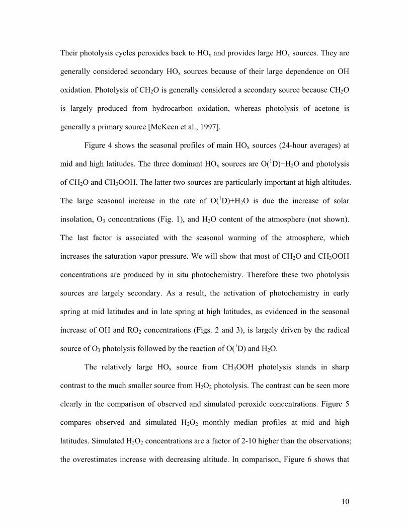
Their photolysis cycles peroxides back to HOx and provides large HOx sources. They are

generally considered secondary HOx sources because of their large dependence on OH

oxidation. Photolysis of CH2O is generally considered a secondary source because CH2O

is largely produced from hydrocarbon oxidation, whereas photolysis of acetone is

generally a primary source [McKeen et al., 1997].

Figure 4 shows the seasonal profiles of main HOx sources (24-hour averages) at

mid and high latitudes. The three dominant HOx sources are O(1D)+H2O and photolysis

of CH2O and CH3OOH. The latter two sources are particularly important at high altitudes.

The large seasonal increase in the rate of O(1D)+H2O is due the increase of solar

insolation, O3 concentrations (Fig. 1), and H2O content of the atmosphere (not shown).

The last factor is associated with the seasonal warming of the atmosphere, which

increases the saturation vapor pressure. We will show that most of CH2O and CH3OOH

concentrations are produced by in situ photochemistry. Therefore these two photolysis

sources are largely secondary. As a result, the activation of photochemistry in early

spring at mid latitudes and in late spring at high latitudes, as evidenced in the seasonal

increase of OH and RO2 concentrations (Figs. 2 and 3), is largely driven by the radical

source of O3 photolysis followed by the reaction of O(1D) and H2O.

The relatively large HOx source from CH3OOH photolysis stands in sharp

contrast to the much smaller source from H2O2 photolysis. The contrast can be seen more

clearly in the comparison of observed and simulated peroxide concentrations. Figure 5

compares observed and simulated H2O2 monthly median profiles at mid and high

latitudes. Simulated H2O2 concentrations are a factor of 2-10 higher than the observations;

the overestimates increase with decreasing altitude. In comparison, Figure 6 shows that

10

simulated CH3OOH concentrations are generally in agreement with the observations.

Using the rate constant of the HO2 self reaction suggested recently by Christensen et al.

[2002], we find that simulated H2O2 concentrations decrease by 20-30% at 6-8 km and 5-

15% at 0-4 km; the large model overestimates remain. The new rate constant has little

effects on simulated OH and HO2 concentrations.

The measurement-model agreement of CH3OOH at mid latitudes is, however, not

as good as those found in the tropics [Wang et al., 2000, 2001]. Particularly noteworthy is

that simulated CH3OOH profiles have a consistent tendency of decreasing with altitude,

which is in accordance with the observed profiles of RO2 concentrations (Fig. 3). The

observed CH3OOH profiles, however, show this altitude dependence in some months but

not in others. In particular, the observed profile at mid latitudes in March shows

increasing concentrations with altitude, opposite to the trend simulated in the model,

resulting in large discrepancies between observed and simulated values. The model

underestimate at 5-8 km is particularly large considering that the model overestimates

peroxy radical concentrations in that month (Fig. 3). The photochemical lifetime of

CH3OOH is generally several weeks or longer during TOPSE. We examined the 10-day

backtrajectories (courtesy of A. Wimmers and J. Moody). Above 4 km, the general flow

is controlled by strong westerlies. Some enhancements of CH3OOH are possible in the

upper troposphere due to vertical transport in the upstream regions [e.g., Prather and

Jacob, 1997]. Wang et al. [2001] estimated that the convective enhancement of CH3OOH

over the tropical Pacific during PEM-Tropics B is only 50-150 pptv (above 10 km)

despite the short convective turnover timescale of 10 days. The concentration of

CH3OOH in the tropical marine boundary is about 1 ppbv. In that work, concentrations of

11

CH3OOH are lowered by up to 100 pptv at 4-7 km due in part to the subsidence of lower

concentrations from higher altitudes. Considering that boundary layer CH3OOH

concentrations in the TOPSE region are only 200-300 pptv, the likely source for high

CH3OOH air masses to the region is from convective transport over the Pacific. The

backtrajectory analysis shows, however, flow patterns in April and May similar to that in

March. We also examined other chemical tracers but did not find clear signals

implicating strong influence by marine air masses in March. The overestimates at 0-4 km

may reflect peroxy radical depletion by fresh NO emissions in the upstream flow from

western United States and Canada. A chemistry and transport model will be necessary to

explore further the causes for the observed vertical trend of CH3OOH at mid latitudes in

March.

At first glance, the large overestimates of H2O2 concentrations but not CH3OOH

might be due to wet scavenging, which efficiently removes soluble H2O2 but not

CH3OOH. Wang et al. [2001] showed convective scavenging over the tropical Pacific

decreases H2O2 concentrations by about 30%. Estimating the magnitude of wet

scavenging on the basis of meteorological measurements during TOPSE is difficult.

Instead we compare the degree of heterogeneous loss of two soluble tracers, H2O2 and

HNO3. Concentrations of HNO3 are also overestimated in the model (not shown). Figure

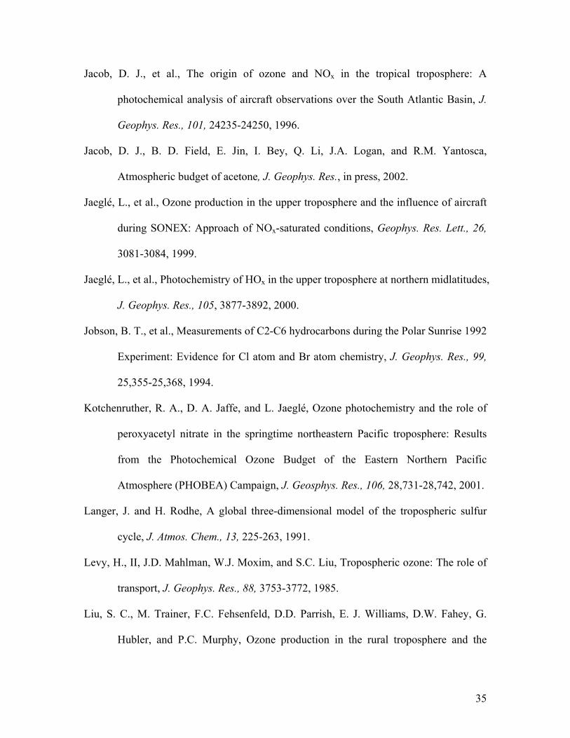
7 shows the seasonal progression of photochemical lifetimes of the two species through

the spring at mid and high latitudes. The photochemical lifetimes are getting shorter into

the summer because of increasing photochemical activity. The photochemical lifetime of

HNO3 is generally about a factor 10 longer than H2O2. Furthermore, the solubility of

12

HNO3 is higher than H2O2, making HNO3 concentrations more sensitive to wet

scavenging and deposition loss.

Assuming gas phase oxidation (by OH), photolysis, and scavenging are the

pathways for removal of H2O2 and HNO3, we calculate the scavenging timescales

necessary to match the observed concentrations in the model (Fig. 8). The required

timescales for HNO3 scavenging are consistent with known rainout frequency and high

solubility of HNO3. The required scavenging is much faster at mid latitudes than at high

latitudes, reflecting more frequent rainout at mid latitudes. The general trend of

decreasing scavenging with altitude is also consistent with the distribution of rainout. The

timescales of HNO3 against scavenging loss are about 1 week at mid latitudes and 2-4

weeks at high latitudes. Our estimates of HNO3 scavenging timescale are likely the upper

limits since we do not take into account the heterogeneous production of HNO3 by N2O5

hydrolysis on aerosols, which could be significant particularly at mid latitudes [Tie et al.,

this issue]. Nonetheless, the derived timescales are in line with the estimates derived from

a global 3-D study of the observed 210Pb distributions by Balkanski et al. [1993].

The required timescales of H2O2 scavenging are more difficult to understand. First,

the required scavenging frequency of H2O2 is up to a factor of 10 faster than that of

HNO3. In May, the loss by scavenging is about half a day at mid latitudes and 1 day at

high latitudes. Second, the required scavenging frequency of H2O2 is more seasonal than

that of HNO3. The seasonal increase of the former is about a factor of 5 at mid and high

latitudes. In contrast, the scavenging frequency of HNO3 shows no clear seasonal change

at mid latitudes and a much smaller increase (mostly from April to May) at high latitudes.

Simple rainout that applies both to HNO3 and H2O2 cannot explain the different

13

characteristics in the required scavenging frequencies of the two species and the rapid

rates of H2O2 removal at mid latitudes. Similar results for H2O2 scavenging are obtained

when using the rate constant of the HO2 self reaction recommended by Christensen et al.

[2002]. One possible pathway is heterogeneous removal of H2O2 by SO2 oxidation in

droplets [e.g., Hoffmann and Edwards, 1975]. The observed monthly median profiles of

SO2 concentrations (not shown) peak in February and are lowest in May. The

concentrations are generally in the range of 10-60 pptv, which are too low to account for

significant H2O2 loss. Furthermore, considering that the average photochemical steady

state concentrations of H2O2 are > 1 ppbv at mid latitudes from March to May and that

the required scavenging lifetime is < 1 day, the supply of SO2 to the TOPSE region needs

to be > 1 ppbv/day. In terms of the sulfur budget, it implies a SO42- wet deposition rate

for the TOPSE region of > 2.5 g S m-2 yr-1, a rate more than 1 order of magnitude larger

than estimated by Langner and Rodhe [1991]. Other SO2 like compounds are necessary to

explain the derived scavenging rates.

A survey of previous comparisons of simulated and observed H2O2 concentrations

suggests that the rapid scavenging loss required for TOPSE observations is unique. The

box models used in the analyses cited below are similar to the one used in this study and

H2O2 was measured in a similar manner in those field experiments as during TOPSE.

Davis et al. [1996] showed relatively good agreement between simulated and observed

H2O2 during PEM-West A over the western Pacific (September-October). Heterogonous

removal of H2O2 was assumed in that model to have a timescale of 5 days below 4 km

and longer at higher altitude. Jacob et al. [1996] found that the model could account for

most of the observed H2O2 at 0-8 km during TRACE-A over the tropical South Atlantic

14

(September-October). Schultz et al. [1999] found good simulation-measurement

agreement at 2-8 km but the model was too high by a factor of 2 at 0-2 km during PEM-

tropics A over the tropical Pacific (August-September). Jaeglé et al. [2000] showed

reasonable agreement between simulated and observed H2O2 during SONEX over the

North Atlantic (October-November). Unlike in the work by Davis et al. [1996], no

heterogeneous loss of H2O2 was included in the other three works. The latter two studies

included heterogeneous production of H2O2 from HO2 on aerosols. The rate of

heterogeneous production used by Schultz et al. [1999] is H2O dependent with a γ of 0.1

whereas that by Jaeglé et al. [2000] depended only on HO2 and aerosol surface area with

a γ of 0.2. Without the heterogeneous production, model results would be considerably

lower than observations in the work by Jaeglé et al. [2000]. It is unclear what effects

heterogeneous production had in the work by Schultz et al. [1999], particularly how

much it contributed to the model overestimates at 0-2 km. Wang et al. [2000] showed that

a 1-D model with a column convective turnover timescale of 20 days could largely

reproduce the observed profile of H2O2 during PEM-Tropics A.

The required scavenging loss of H2O2 implies rapid removal of a large reservoir

of HOx and consequently slows down the HOx cycles and O3 production. Figure 9 shows

the ratios of 24-hour average HOx production, OH concentrations, and O3 production in

the simulations using observed vs. simulated H2O2 concentrations. The relative effects

are similar at mid and high latitudes and among different months. The decrease of HOx

source from the photolysis of H2O2 leads to a loss of 20-40% in the production of HOx.

The decrease of 20-30% in OH concentrations is larger than that of 10-20% for the

peroxy radicals (not shown), which results in a similar decrease in O3 production. The

15

photochemical loss (and hence the net production or loss) also decreases in a similar

proportion, reflecting the importance of the reaction of O3 and HO2 in O3 loss (section 5).

3.2 CH2O as a large source of HOx at northern high latitudes

Among the HOx sources shown in Fig. 4, the photolysis of CH2O is particularly

large. Relative to the total HOx source, it is larger at higher altitudes and latitudes where

the decrease of H2O vapor concentrations with temperature reduces the source from the

reaction of O(1D) and H2O. This HOx source often reflects the auto-catalytic nature of the

HOx cycles since CH2O is largely produced during the OH oxidation of hydrocarbons.

However, standard gas-phase photochemistry alone cannot explain the observed

CH2O concentrations at high altitudes in northern high latitudes, where CH2O photolysis

is of great importance to the HOx budget. Figure 10 compares model simulated median

profiles of CH2O with observations. Simulated median CH2O concentrations are

generally within the standard deviation of the observed concentrations. Whereas good

agreement was found for mid latitude observations, simulated CH2O concentrations were

much lower at high latitudes in March. These underestimates are particularly large at

higher altitudes. Fried et al. [this issue] further examined the model underestimates and

investigated a number of possibilities that could increase CH2O production at high

latitudes and altitudes, including direct production from the reaction of CH3O2 and HO2

[Ayer et al., 1997], the decomposition of CH3OONO2 [Cantrell et al., this issue], and

heterogeneous conversion of CH3OH to CH2O in aerosols [Singh et al., 2000]. They

found no clear evidence attributing the observed excess CH2O to these pathways.

16

Another hypothesis is mixing between mid and high latitude air masses enhances CH2O

concentrations at high latitudes.

Simulated CH2O concentrations are affected by CH3OOH concentrations [Liu et

al., 1992]. The sensitivity varies. The model underestimates at high altitudes are larger

when model simulated CH3OOH concentrations are used instead of observed CH3OOH

(Fig. 11). The effect is particularly large at 6-8 km in March; using observed in place of

simulated CH3OOH concentrations in the model increases CH2O concentrations by about

50-100% (20-30 pptv). In general, the enhancements are above 4 km; the increase is

about 10-40% in April and May. The assumption used to calculate acetone concentrations

by scaling to CO concentrations is another factor contributing to the uncertainty in the

simulated CH2O concentrations. Jacob et al. [2002] suggested that acetone concentrations

are lower in winter and spring than in the fall due to the loss of acetone to the oceans.

Reducing our estimated acetone concentrations by half matches the levels (300-600 ppbv)

simulated by Jacob et al. [2002] for North America in January. The lowering of acetone

concentrations decreases simulated CH2O concentrations by 10-20% above 5 km, which

will increase the underestimates by the model.

It is unclear if the additional CH2O beyond the level that can be sustained by the

standard gas-phase photochemistry is a primary or secondary source of HOx at high

altitudes since the nature of the model underestimate is unknown. However, we can

examine the various hypotheses more closely. If the additional CH2O is due to transport

or conversion of CH3OH in aerosols, its photolysis increases the primary HOx source. If it

is due to production from the reaction of CH3O2 and HO2 or from CH3OONO2

decomposition, the additional HOx source is secondary. Boosting the secondary HOx

17

source implies more efficient yields of CH2O from hydrocarbon oxidation. Considering

that CH4 oxidation provides about 70-80% of the total CH2O source and that the yield of

CH2O from this oxidation is already close to 1 in the box model (with no heterogeneous

loss of CH3OOH assumed), it is unlikely that these pathways will significantly increase

CH2O concentrations to make up for the large underestimates shown in Figure 10.

Therefore, it is more likely that the additional HOx source from CH2O photolysis is

primary.

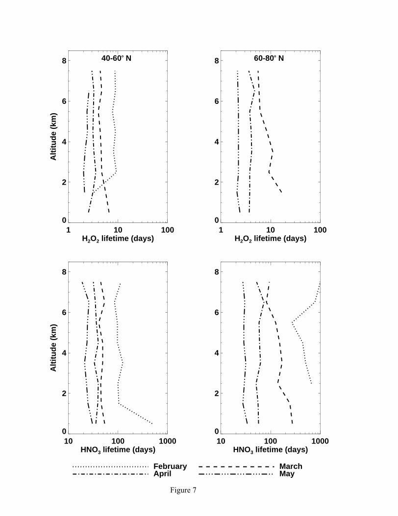
Figure 12 shows the ratios of 24-hour average HOx production, OH

concentrations, and O3 production in the simulations using observed vs. simulated CH2O

concentrations. The effects are significant at high latitudes above 6 km and are larger in

March than in May. The largest effect is seen in the total production of HOx, decreasing

from a factor of 2 to 30% from March to May above 6 km at high latitudes. In the region,

the concentrations of OH and HO2 (not shown) and the production of O3 increase by 20-

50%. The seasonal decrease in the relative contribution of the “excess” CH2O to HOx

reflects in part the increasing contribution from the reaction O(1D) and H2O to the HOx

source with time and in part lesser underestimates by the model in late spring [Fried et al.,

this issue]. The effects are minimal at mid latitudes where simulated and observed CH2O

concentrations are in better agreement. Photolysis of acetone also affects HOx chemistry

at high altitudes [e.g., McKeen et al., 1997]. During the TOPSE period, it is not the

dominant HOx sources (Fig. 4). Reducing acetone concentrations estimated in the model

by half decreases HOx production by up to 12 and 20% at mid and high latitudes (> 6 km),

respectively. The effects on the concentration of OH and O3 production are around 10%

18

at altitude above 6 km. The effects are insignificant below 4 km where the source from

the reaction of O(1D) and H2O dominates HOx production.

4. Nitrogen oxides and in situ O3 production

Figure 13 compares simulated and observed monthly median profiles of NO2 at

mid and high latitudes. Although the simulated median profiles of NO2 at given altitude

bins are within the observed monthly standard deviations, which are often larger than the

scale of the plots and are hence not shown, simulated NO2 concentrations tend to be

lower than the observations. The underestimates are largest above 6 km (about 10 pptv).

Some of the discrepancies can be attributed to the measurement uncertainty, which

increases with altitude from 3 pptv to 8 pptv. The increasing measurement uncertainties

with altitude are also reflected in the increasing proportion of data near the detection

limits, reaching 50% at 6-8 km. The model overestimate at 1-2 km in February at mid

latitudes is due to some high concentration plumes sampled by the C-130. On the basis of

observed NO concentrations, the model predicts broader plumes than found in the NO2

measurements. When model points with no corresponding NO2 measurements are

included, the median model value drops to 25 pptv and is in agreement with the

observations. The seasonal increase of NO concentrations during TOPSE is shown in

Figure 1. In comparison, the seasonal increase of NO2 is much smaller, reflecting the

shift of NOx partition towards NO as photolysis of NO2 increases with time.

Jaeglé et al. [1999] mapped O3 production as a function of the primary source of

HOx and NOx concentration for the observations during SONEX. Figure 14 shows the

mapping for TOPSE observations, where the primary HOx source is driven mostly by the

reaction of O(1D) and H2O. Compared with SONEX, two features stand out. Firstly, there

19

is a clear positive correlation between primary HOx production and NOx concentrations,

whereas Jaeglé et al. [1999] found marine convected air masses (over the North Atlantic)

with high primary HOx production but low NOx concentrations during SONEX. During

TOPSE, the positive correlation reflects the convergence of favorable photochemical

environment (Fig. 4) and increasing NOx concentrations. Secondly, in the same range of

primary HOx production rates and NOx concentrations, the O3 production rates are similar

between TOPSE and SONEX despite that our work is for 0-8 km in spring and the work

by Jaeglé et al. [1999] is for 8-12 km in the fall.

A casual look of the first panel of Figure 14 would suggest that the primary HOx

production does not play a significant role in the production rate of O3. Part of the

insensitivity of O3 production to the primary HOx source is due to the rapid increase of

NO/NO2 ratio with altitude, which is driven by the temperature dependence of the NO +

O3 reaction and the altitude dependence of air density and photon flux. The same amount

of NOx is therefore more effective in O3 production at high altitudes where NO/NO2 ratio

is high since the production is driven by the reaction of NO with peroxy radicals. This

effect combined with a decreasing trend of the HOx primary production with altitude

tends to mask the contribution of the primary HOx source to O3 production.

We therefore mapped O3 production as a function of NO in Figure 14 as well. At

NO levels above 10 pptv, it is clear that increasing the primary HOx source enhances O3

production. Considering that the range of the primary HOx source spans about 4 orders of

magnitudes, the efficiency of primary HOx production in boosting O3 production (∂P(O3)/

∂P(HOx)) is less than that of NOx (or NO). However, it should be noted that the increase

of primary HOx production through the spring is much more rapid than that of NO (Figs.

20

1 and 4). The large dependence of O3 production on NO concentrations reflects a NOx-

limited photochemical regime during TOPSE.

5. Budgets of reactive nitrogen and O3

Penkett and Brice [1986] used the rapid buildup and loss of peroxyacetylnitrate

(PAN) at a rural site in spring as a proxy to suggest that intensifying photochemistry

activity contributes to the observed springtime O3 maximum. Honrath et al. [1996]

further suggested that the accumulation of reactive nitrogen at winter high latitudes and

the subsequent decomposition of these reservoirs back to NOx in spring could contribute

to the observed springtime maximum.

Figure 15 shows the monthly median profiles of total reactive nitrogen (NOy) and

PAN concentrations at mid and high latitudes. The most abundant NOy component is

PAN accounting for 40-80% of NOy. The PAN fraction in NOy decreases with season.

The continually increasing concentrations of NOy and PAN in the most part of the

troposphere show no evidence for wintertime accumulation at high latitudes followed by

springtime transport to mid latitudes. Free tropospheric measurements are particularly

important in understanding the seasonality of reactive nitrogen species at mid and high

latitudes because the seasonal trends are quite different near the surface from that in the

free troposphere. Concentrations of NOy and PAN above 3 km continue to increase

throughout the spring. The seasonal trend at lower altitudes is not as well defined as that

at higher altitudes. The concentrations of NOy tend to peak in February near the surface;

the seasonal maximum of PAN near the surface is shifted towards April particularly at

mid latitudes.

21

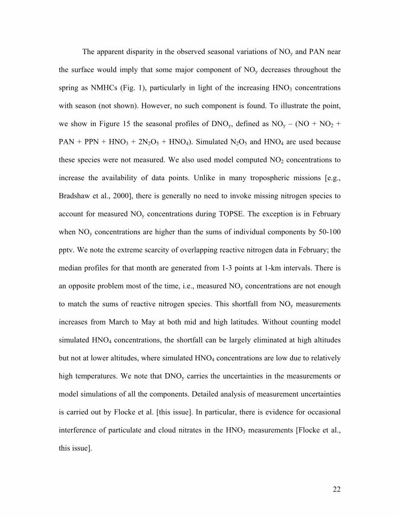
The apparent disparity in the observed seasonal variations of NOy and PAN near

the surface would imply that some major component of NOy decreases throughout the

spring as NMHCs (Fig. 1), particularly in light of the increasing HNO3 concentrations

with season (not shown). However, no such component is found. To illustrate the point,

we show in Figure 15 the seasonal profiles of DNOy, defined as NOy – (NO + NO2 +

PAN + PPN + HNO3 + 2N2O5 + HNO4). Simulated N2O5 and HNO4 are used because

these species were not measured. We also used model computed NO2 concentrations to

increase the availability of data points. Unlike in many tropospheric missions [e.g.,

Bradshaw et al., 2000], there is generally no need to invoke missing nitrogen species to

account for measured NOy concentrations during TOPSE. The exception is in February

when NOy concentrations are higher than the sums of individual components by 50-100

pptv. We note the extreme scarcity of overlapping reactive nitrogen data in February; the

median profiles for that month are generated from 1-3 points at 1-km intervals. There is

an opposite problem most of the time, i.e., measured NOy concentrations are not enough

to match the sums of reactive nitrogen species. This shortfall from NOy measurements

increases from March to May at both mid and high latitudes. Without counting model

simulated HNO4 concentrations, the shortfall can be largely eliminated at high altitudes

but not at lower altitudes, where simulated HNO4 concentrations are low due to relatively

high temperatures. We note that DNOy carries the uncertainties in the measurements or

model simulations of all the components. Detailed analysis of measurement uncertainties

is carried out by Flocke et al. [this issue]. In particular, there is evidence for occasional

interference of particulate and cloud nitrates in the HNO3 measurements [Flocke et al.,

this issue].

22

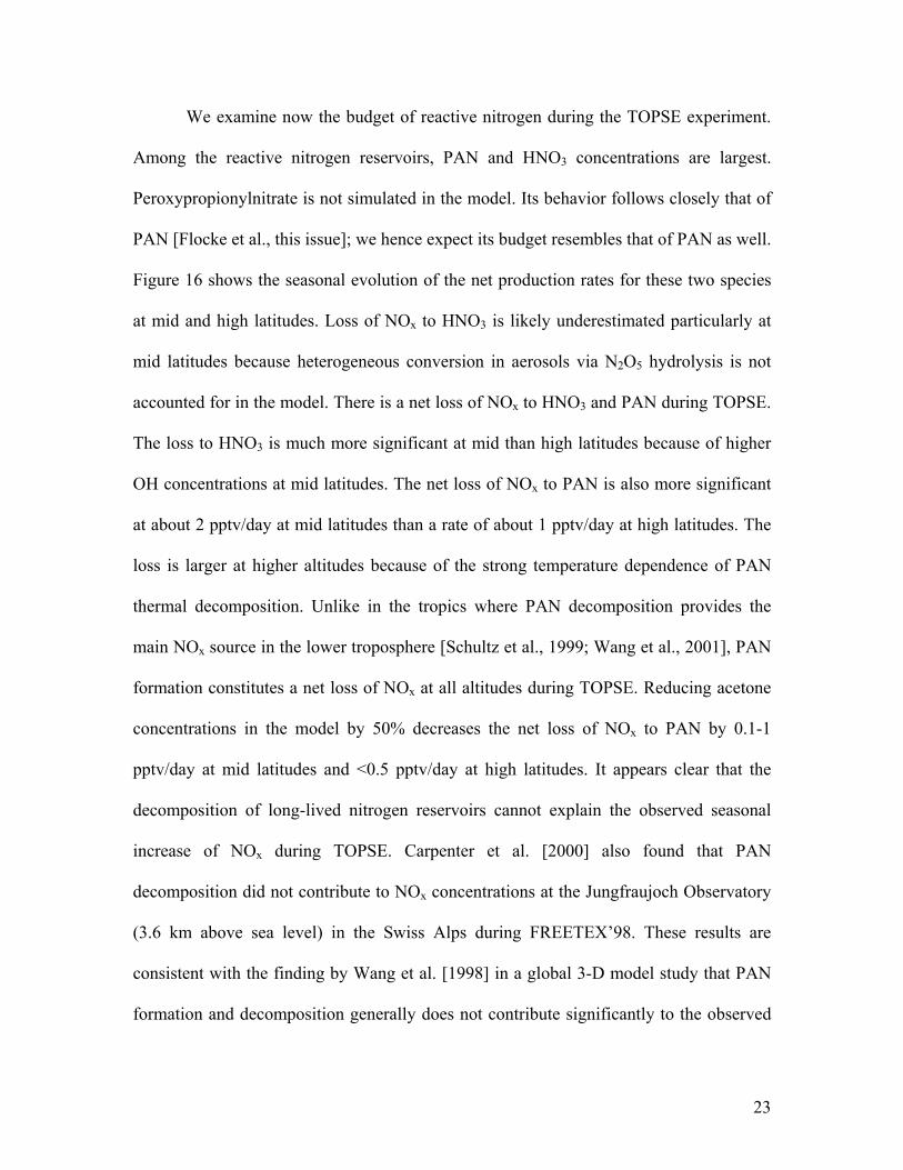
We examine now the budget of reactive nitrogen during the TOPSE experiment.

Among the reactive nitrogen reservoirs, PAN and HNO3 concentrations are largest.

Peroxypropionylnitrate is not simulated in the model. Its behavior follows closely that of

PAN [Flocke et al., this issue]; we hence expect its budget resembles that of PAN as well.

Figure 16 shows the seasonal evolution of the net production rates for these two species

at mid and high latitudes. Loss of NOx to HNO3 is likely underestimated particularly at

mid latitudes because heterogeneous conversion in aerosols via N2O5 hydrolysis is not

accounted for in the model. There is a net loss of NOx to HNO3 and PAN during TOPSE.

The loss to HNO3 is much more significant at mid than high latitudes because of higher

OH concentrations at mid latitudes. The net loss of NOx to PAN is also more significant

at about 2 pptv/day at mid latitudes than a rate of about 1 pptv/day at high latitudes. The

loss is larger at higher altitudes because of the strong temperature dependence of PAN

thermal decomposition. Unlike in the tropics where PAN decomposition provides the

main NOx source in the lower troposphere [Schultz et al., 1999; Wang et al., 2001], PAN

formation constitutes a net loss of NOx at all altitudes during TOPSE. Reducing acetone

concentrations in the model by 50% decreases the net loss of NOx to PAN by 0.1-1

pptv/day at mid latitudes and <0.5 pptv/day at high latitudes. It appears clear that the

decomposition of long-lived nitrogen reservoirs cannot explain the observed seasonal

increase of NOx during TOPSE. Carpenter et al. [2000] also found that PAN

decomposition did not contribute to NOx concentrations at the Jungfraujoch Observatory

(3.6 km above sea level) in the Swiss Alps during FREETEX’98. These results are

consistent with the finding by Wang et al. [1998] in a global 3-D model study that PAN

formation and decomposition generally does not contribute significantly to the observed

23

springtime O3 maxima over northern mid and high latitude continents. More

measurements are necessary to understand if and how the NOx source from PAN

decomposition in remote marine regions and lower latitudes contributes to the seasonal

variability of ozone.

The seasonal increases of NO and primary HOx production (Figs. 1 and 4) result

in increasing chemical production of O3 (Fig. 14). Figure 17 shows the budgets of O3 at

mid and high latitudes. The model is not constrained by observed peroxides or CH2O

because the restriction would reduce available data points so severely that no statistically

meaningful column budget can be obtained. The comparison of the simulations with and

without the constraints shows that the effect of the scavenging loss of H2O2 is larger than

those of higher than simulated (“excess”) CH3OOH and CH2O concentrations in the

observations. The resulting effects are similar (10-20% overestimates) for O3 production,

loss, and net production (loss).

Figure 17 shows the rapid increase of O3 production throughout the spring. The

increase is more rapid at high latitudes (by a factor of 2-3 per month) than at mid

latitudes (decreasing from a factor of 2 in February-March to 50% in April-May). By

May, O3 column production rates (0-8 km) are 3.2x1011 and 2.3x1011 cm-2 s-1 for mid and

high latitudes, respectively. About 70% of O3 production is due to the reaction of HO2

and NO, and the rest is by the reactions of NO with CH3O2 and other organic peroxy

radicals. The source from the reactions of NO and other organic peroxy radicals are

significant compared to that from the reaction of NO and CH3O2 in early spring. The

relative strengths of the two sources changes from 1:1 (1:2) in February to 1:3 (1:4) in

May at high (mid) latitudes, reflecting the decrease of NMHCs with season (Fig. 1). Our

24

rate estimates are less than those calculated by Cantrell et al. [this issue]; the former

values are 24-hour averages while the latter ones are instantaneous rates at the time of the

observations.

The ozone budget at mid latitudes can be compared with the estimates for the

western north Pacific (30-50° N) in February-March (1994) by Crawford et al. [1997].

They found much larger column O3 production (10.5x1010 cm-2 s-1) than loss (3.8x1010

cm-2 s-1). Their production rate is similar to our estimate for March but their loss rate is

similar to our estimate in February. As a result, their estimated column net production is

much larger than our estimate. The discrepancy is due in part to higher O3 concentrations

(~ 20 ppbv) during TOPSE. One important similarity between the two studies is that the

lower free troposphere (1-4 km) is a significant region of net O3 production. Crawford et

al. [1997] attributed the enhanced O3 production at these altitudes to continental outflow

to the western Pacific.

The dominant role that HO2 plays in O3 loss rates is shown in Figure 18. The

largest loss of O3 in the tropical and subtropical regions is due to photolysis of O3 and the

subsequent reaction of O(1D) and H2O [e.g., Davis et al. 1996; Jacob et al., 1996]. In

comparison, during TOPSE the largest loss of O3 is from the reaction of O3 and HO2. At

mid latitudes, that loss accounts for 70% of the total O3 loss in February and a smaller

45% in May. Kotchenruther et al. [2001] reported a fraction of about 60% in April over

the north eastern Pacific. The fractional contribution by the reaction of O3 and HO2 at

high latitudes decreases from 90% in February to 70% in May. The highest contribution

by the reaction of O(1D) and H2O is 35% at mid latitudes in May. The small fractional

contribution to O3 loss by the reaction of O(1D) and H2O reflects much drier air and less

25

solar insolation over the TOPSE region compared to the lower latitudes. The crucial role

played by HO2 in both O3 production and loss explains the similar sensitivities of these

variables to a change in the HOx source.

The relatively small loss of O3 by the reaction of O(1D) and H2O helps limit O3

loss at northern mid and high latitudes in spring, resulting in a net chemical production of

O3 at mid latitudes during TOPSE. At mid latitudes, the net column chemical production

is 2x1010, 1x1010, 4x1011, and 1x1011 cm-2 s-1 for February, March, April, and May

respectively. The corresponding values at high latitudes are -6x108, -4x109, -1x1010, and

3x1010 cm-2 s-1. The net loss in February-April at high latitudes reflects the low NOx

concentrations (< 5 pptv below 5 km) in the region (Fig. 1). The net chemical production

or loss is only 3-20% of the column O3 production or loss rate at 0-8 km. The

combination of high NO concentrations and low H2O content leads to net O3 production

at high altitudes. Including the net O3 production in the region between 8 km and the

tropopause will further increase the estimated net chemical production of O3.

Figure 19 shows that the median column O3 concentration (defined as column

moles of O3/column moles of air) at mid latitudes is highest in April and that the most

rapid O3 increase occurs in March-April, a period when the springtime O3 maxima were

observed at lower altitudes at mid and high latitudes [e.g., Logan et al. 1985; Levy et al.,

1985]. The estimated net O3 production is also largest in April. In contrast, at high

latitudes during TOPSE, column O3 concentrations continue to increase from February to

May and there is an estimated chemical loss of O3 from February to April. To illustrate

the different effects of in situ net O3 chemical production (loss) on column O3

concentrations at mid and high latitudes, we show in Figure 19 the column concentrations

26

of O3 for March, April, and May if in situ chemistry is the only factor influencing the

concentrations (see also the figure caption). The estimated column O3 at mid latitudes

does not show a maximum in April because the in situ chemical production is still larger

than loss in May. Nonetheless, the estimated concentrations reach the observed levels at

mid latitudes. In comparison, the estimated O3 concentrations at high latitudes remain at

about 50 ppbv due to the relatively small net production or loss in that region, whereas

the observed column mixing ratio increases by 15 ppbv.

In situ chemistry alone cannot explain the observed springtime O3 maxima at

northern mid and high latitudes; transport plays an important role. Wang et al. [1998]

tagged O3 transported from the stratosphere and that produced in different regions of the

troposphere in a global 3-D chemistry and transport model. They found that O3 from the

stratosphere peaked in late winter and early spring whereas O3 produced from the

troposphere peaked in late spring and early summer. Both sources are important in

reproducing the observed springtime O3 maxima at remote northern mid and high latitude

sites in their model. Yienger et al. [1999] emphasized the role played by the net O3

chemical production at mid latitudes, which we find to be important for the TOPSE

region. Their simulated net chemical O3 production (2-10 km) at mid latitudes peaks in

March, one month earlier than we find for the TOPSE region. The two results, however,

cannot be directly compared because their results include all regions at 30-60° N. In our

current work, we focused only on the effects of in situ chemical production and loss

during TOPSE. Detailed analysis of tropospheric and stratospheric O3 transport into the

TOPSE region is presented by Allen et al. [this issue], Browell et al. [this issue], Dibb et

al. [this issue], Emmons et al. [this issue], and Wang et al. [2002].

27

6. Conclusions

Measurements were made onboard the NCAR/NSF C-130 aircraft in February-

May during the TOPSE experiment at northern mid and high latitudes. The temporal and

spatial span of the measurements allows for analysis of the rapid transition of

photochemistry in springtime using a photochemical model. We have focused our work

on photochemical factors driving HOx and O3 chemistry.

The continuously decreasing concentrations of NMHCs through spring, due in

part to increasing OH oxidation, contrast to the observed increase in O3 and NO

concentrations. Both trends favor partitioning of HOx towards OH. Photochemical

activity as measured by the sources of HOx increases rapidly at mid and high latitudes

with season. The primary driving force for radical chemistry is photolysis of O3 and the

subsequent reaction of O(1D) and H2O, which benefits not only from the increasing solar

insolation but higher H2O content of the warming air. The concentrations of total peroxy

radicals rise accordingly; observed and simulated concentrations are in good agreement.

One feature that sets TOPSE apart from the other tropospheric field experiments

is the observations of low H2O2 concentrations (by a factor of 2-10) compared to model

estimates. The loss of HOx required to match observed H2O2 concentrations in the model

implies a loss of 20-30% and 10-20% in OH concentrations and O3 production,

respectively. The timescale of scavenging by rainout, calculated from the observed HNO3

concentrations, increases from about 1 week at mid latitudes to 2-4 weeks at high

latitudes in agreement with previous estimates. However, the required scavenging loss

frequency of H2O2 is much faster. Furthermore, it increases rapidly with season. The

estimated timescales of H2O2 against scavenging loss in May are about half a day and 1

28

day at mid and high latitudes, respectively. If the scavenging loss of H2O2 were mostly

due to its oxidation of SO2 in droplets, the oxidation would imply a sulfate deposition rate

of > 2.5 g S m-2 yr-1, an order of magnitude larger than previous estimates. Unknown

mechanisms need to be invoked to explain the rapid loss of H2O2 during TOPSE.

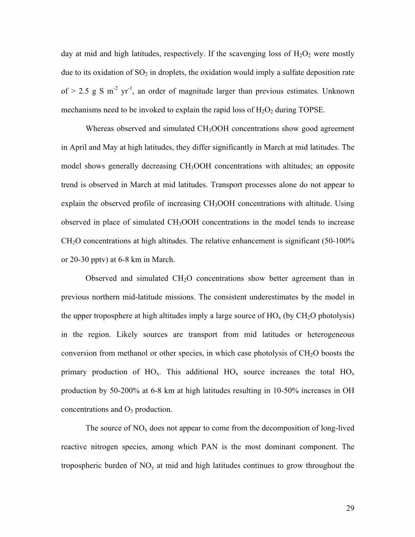
Whereas observed and simulated CH3OOH concentrations show good agreement

in April and May at high latitudes, they differ significantly in March at mid latitudes. The

model shows generally decreasing CH3OOH concentrations with altitudes; an opposite

trend is observed in March at mid latitudes. Transport processes alone do not appear to

explain the observed profile of increasing CH3OOH concentrations with altitude. Using

observed in place of simulated CH3OOH concentrations in the model tends to increase

CH2O concentrations at high altitudes. The relative enhancement is significant (50-100%

or 20-30 pptv) at 6-8 km in March.

Observed and simulated CH2O concentrations show better agreement than in

previous northern mid-latitude missions. The consistent underestimates by the model in

the upper troposphere at high altitudes imply a large source of HOx (by CH2O photolysis)

in the region. Likely sources are transport from mid latitudes or heterogeneous

conversion from methanol or other species, in which case photolysis of CH2O boosts the

primary production of HOx. This additional HOx source increases the total HOx

production by 50-200% at 6-8 km at high latitudes resulting in 10-50% increases in OH

concentrations and O3 production.

The source of NOx does not appear to come from the decomposition of long-lived

reactive nitrogen species, among which PAN is the most dominant component. The

tropospheric burden of NOy at mid and high latitudes continues to grow throughout the

29

spring. This seasonal increase is clearly evident in the free troposphere. The seasonality is

less clearly defined at 0-3 km. The concentrations of NOy near the surface decrease from

February to May (particularly at high latitudes) as those of NMHCs. Similar difference of

the seasonal trend with altitude is observed for PAN except that the seasonal peak of

PAN near the surface shifts towards April. Budget studies of PAN and HNO3 show a net

loss of NOx to these reservoirs species throughout the spring. There appears to be a

seasonal shift in the difference between NOy and the sum of individual components (NO

+ NO2 + PAN + PPN + HNO3 + 2N2O5 + HNO4), among which NO2, N2O5, and HNO4

are computed in the model. The former is larger in February but becomes progressively

smaller than the latter in later months. The shift shows little altitude dependence.

The production of O3 in the TOPSE region increases substantially from February

to May, by factors of 5 and 25 respectively at mid and high latitudes. The rapid increase

is driven by increasing primary HOx production and NO concentrations. The latter is due

in part to the increasing partitioning of NOx towards NO with more intense solar

irradiation in spring. Ozone production is less sensitive to an increase in the primary HOx

production than that in NO concentrations. However, the former factor, driven by the

reaction of O(1D) and H2O, increases more rapidly than the latter. Ozone photochemistry

is in the NOx-limited regime during TOPSE.

Peroxy radicals generally play the pivotal role in O3 production. The reaction of

HO2 and NO accounts for about 70% of the total production. The contribution by the

reaction of higher (≥ C2) organic peroxy radicals and NO is as large as that by the

reaction of CH3O2 and NO in early spring, reflecting the high concentrations of NMHCs

at the time. Its relative importance decreases towards summer. During TOPSE, HO2 is

30

also the major component in O3 loss through the reaction of HO2 and O3. The loss

pathway accounts for 45-70% and 70-90% of the total loss at mid and high latitudes,

respectively. The loss pathway by photolysis of O3 and the subsequent reaction of O(1D)

and H2O, which dominates O3 loss at lower latitudes, is highest (35%) at mid latitudes in

May. As a result, the sensitivities of O3 production and loss to a change in the primary

HOx production are similar.

We find net in situ column O3 chemical production (0-8 km) at mid latitudes,

2x1010, 1x1010, 4x1011, and 1x1011 cm-2 s-1 for February, March, April, and May

respectively. In contrast, there is a net in situ chemical loss of O3 at high latitudes except

in May. The corresponding values at high latitudes are -6x108, -4x109, -1x1010, and

3x1010 cm-2 s-1. The difference reflects lower NO concentrations and solar irradiation at

high latitudes. At mid latitudes, the lower free troposphere (1-4 km) in addition to the

upper troposphere is a region of significant net O3 production. The observed O3 column

(0-8 km) shows a peak in April at mid latitudes but continues to increase from February

to May at high latitudes. In situ chemistry alone cannot explain the observed seasonality

of column O3 during TOPSE. Nonetheless, in situ net chemical production is a significant

contributor to the observed O3 increase at mid latitudes, where both net O3 production

and column concentration peak in April. Net transport from other tropospheric regions or

the stratosphere is necessary to explain the observed seasonal increase of column O3 at

high latitudes.

Acknowledgements:

31

We thank Luca Cinquini and Lousia Emmons at NCAR for their excellent work

in data management and for sending us various data products. We also thank Anthony

Wimmers and Jennie Moody at the University of Virginia for providing their

backtrajectory analysis. The operation of C-130 aircraft during TOPSE was managed by

the Research Aviation Facility of NCAR. This work is supported by the National Science

Foundation (grant ATM-0000337).

References

Allen, D., et al., An estimate of the stratospheric input to the troposphere during TOPSE

using 7Be measurements and model simulations, this issue.

Atkinson, R., et al., Evaluated kinetic and photochemical data for atmospheric chemistry,

J. Phys. Chem. Ref. Data, 26, suppl. VI, 1329-1499, 1997.

Atlas, E., et al., The TOPSE Experiment: Introduction, this issue.

Ayers, G.P, R.W. Gillett, H. Granek, C. de Serves, and R.A. Cox, Formaldehyde

production in clean marine air, Geophys. Res. Lett., 24, 401– 404, 1997.

Balkanski, Y. J., D. J. Jacob, G. M. Gardner, W. M. Graustein, and K. K. Turekian,

Transport and residence times of continental aerosols inferred from a global 3-

dimensional simulation of 210Pb, J. Geophys. Res., 98, 20573-20586, 1993.

Blake, N. J., et al., The seasonal evolution of NMHCs and light alkyl nitrates at mid to

high northern latitudes during TOPSE, this issue.

Bottenheim, J.W., and M. F. Shepherd, C2-C6 Hydrocarbon measurements at 4 rural

locations across Canada, Atmos. Environ., 29, 647-664 , 1995.

32

Bradshaw, J., et al., Observed distributions of nitrogen oxides in the remote free

troposphere from the NASA Global Tropospheric Experiment programs, Rev.,

Geophys., 38, 61-116, 2000.

Browell, E. et al., Ozone, aerosol, potential vorticity, and trace gas trends observed at

high latitudes from February to May 200, this issue.

Cantrell, C., et al. Steady state free radical budgets and ozone photochemistry during

TOPSE, this issue.

Carpenter, L. J., et al., Oxidized nitrogen and ozone production efficiencies in the

springtime free troposphere over the Alps, J. Gephys. Res., 105, 14,547-14,559,

2000.

Chen, G., et al., An assessment of HOx chemistry in the tropical Pacific boundary layer:

Comparison of observations with model simulations during PEM Tropics A, J.

Atm. Chem., 38, 317-344, 2001.

Christensen, L. E., M. Okumura, S. P. Sander, R. J. Salawitch, G. C. Toon, B. Sen, J.-F.

Blavier, and K. W. Jucks, Kinetics of HO2 + HO2 → H2O2 + O2: Implications for

stratospheric H2O2, Geophys. Res. Lett., in press, 2002.

Crawford, J. H., et al., An assessment of ozone photochemistry in the extratropical

western North Pacific: Impact of continental outflow during the late winter/early

spring, J. Geophys. Res., 102, 28,469-28,487, 1997.

Crawford, J. H., et al. Assessment of upper tropospheric HOx sources, J. Geophys. Res.,

104, 16,255-16,273, 1999.

33

Davis, D. D., et al., Assessment of the ozone photochemistry tendency in the western

North Pacific as inferred from PEM-West A observations during the fall of 1991,

J. Geophys. Res., 101, 2111-2134, 1996.

Davis, D. D., et al., Marine latitude/altitude OH distributions: Comparison of Pacific

Ocean observations with models, J. Geophys. Res., 106, 32,691-32,708, 2001.

DeMore, W. B., et al., Chemical kinetics and photochemical data for use in stratospheric

modeling, JPL Publ. 97-4, 266 pp., 1997.

Dibb, J., et al., Stratospheric influence on the northern North American free troposphere

during TOPSE: 7Be as a stratospheric tracer, this issue.

Emmons, L. K., et al., The budget of tropospheric ozone during TOPSE from two CTMs,

this issue.

Flocke et al., The behavior of PAN and the balance of odd nitrogen during TOPSE, this

issue.

Fried et al., Tunable diode laser measurements of formaldehyde during the TOPSE 2000

study: Distributions, trends, and model comparisons, this issue.

Hoffmann, M. R., and J. O., Edwards, Kinetics of oxidation of sulfite by hydrogen

peroxide in acidic solution, J. Phys. Chem., 79, 2096-2098, 1975.

Honrath, R.E., and D.A. Jaffe, The seasonal cycle of nitrogen oxides in the Arctic

troposphere at Barrow, Alaska, J. Geophys. Res., 97, 20615-10630, 1992.

Honrath, R.E., A.J. Hamlin, and J.T. Merrill, Transport of ozone precursors from the

Arctic troposphere to the North Atlantic region, J. Geophys. Res., 101, 29335-

29351, 1996.

34

Jacob, D. J., et al., The origin of ozone and NOx in the tropical troposphere: A

photochemical analysis of aircraft observations over the South Atlantic Basin, J.

Geophys. Res., 101, 24235-24250, 1996.

Jacob, D. J., B. D. Field, E. Jin, I. Bey, Q. Li, J.A. Logan, and R.M. Yantosca,

Atmospheric budget of acetone, J. Geophys. Res., in press, 2002.

Jaeglé, L., et al., Ozone production in the upper troposphere and the influence of aircraft

during SONEX: Approach of NOx-saturated conditions, Geophys. Res. Lett., 26,

3081-3084, 1999.

Jaeglé, L., et al., Photochemistry of HOx in the upper troposphere at northern midlatitudes,

J. Geophys. Res., 105, 3877-3892, 2000.

Jobson, B. T., et al., Measurements of C2-C6 hydrocarbons during the Polar Sunrise 1992

Experiment: Evidence for Cl atom and Br atom chemistry, J. Geophys. Res., 99,

25,355-25,368, 1994.

Kotchenruther, R. A., D. A. Jaffe, and L. Jaeglé, Ozone photochemistry and the role of

peroxyacetyl nitrate in the springtime northeastern Pacific troposphere: Results

from the Photochemical Ozone Budget of the Eastern Northern Pacific

Atmosphere (PHOBEA) Campaign, J. Geosphys. Res., 106, 28,731-28,742, 2001.

Langer, J. and H. Rodhe, A global three-dimensional model of the tropospheric sulfur

cycle, J. Atmos. Chem., 13, 225-263, 1991.

Levy, H., II, J.D. Mahlman, W.J. Moxim, and S.C. Liu, Tropospheric ozone: The role of

transport, J. Geophys. Res., 88, 3753-3772, 1985.

Liu, S. C., M. Trainer, F.C. Fehsenfeld, D.D. Parrish, E. J. Williams, D.W. Fahey, G.

Hubler, and P.C. Murphy, Ozone production in the rural troposphere and the

35

implications for regional and global ozone distributions, J. Geophys. Res., 92,

10463-10482, 1987.

Liu, S. C., et al., A study of the photochemistry and ozone budget during the Mauna Loa

Observatory Photochemistry Experiment, J. Geophys. Res., 97, 10,463 – 10,471,

1992.

Logan, J.A., M.J. Prather, S.C. Wofsy, and M.B. McElroy, Tropospheric chemistry: A

global perspective, J. Geophys. Res., 86, 7210-7254, 1981.

Logan, J.A., Tropospheric ozone: Seasonal behavior, trends, and anthropogenic influence,

J. Geophys. Res., 90, 10463-10482, 1985.

McKeen, S. A., et al., Photochemical modeling of hydroxyl and its relationship to other

species during the tropospheric OH photochemistry experiment, J. Geophys. Res.,

102, 6467-6493, 1997.

Novelli, P.C., J.E. Collins, Jr., R.C. Myers, G.W. Sachse, and H.E. Scheel, Re-evaluation

of the NOAA/CMDL carbon monoxide reference scale and comparisons to CO

reference gases at NASA-Langley and the Fraunhofer Institute, J. Geophys. Res.,

99, 12833-12839, 1994.

Penkett, S.A., and K.A. Brice, The spring maximum in photo-oxidants in the Northern

Hemisphere troposphere, Nature, 319, 655-657, 1986.

Prather, M. J., and D. J. Jacob, A persistent imbalance in HOx and NOx photochemistry of

the upper troposphere driven by deep tropical convection, Geophys. Res. Lett., 24,

3189-3192, 1997.

Schultz, M., et al., On the origin of tropospheric ozone and NOx over the tropical South

Pacific, J. Geophys. Res., 104, 5829-5843, 1999.

36

Shetter, R. E., L. Cinquini, B. L. Lefer, S. R. Hall, and S. Madronich, Comparison of

airborne measured and calculated spectral actinic flux and derived photolysis

frequencies during the PEM Tropics B mission, J. Geophys. Res., in press, 2002.

Singh, H., et al., Distribution and fate of selected oxygenated organic species in the

troposphere and lower stratosphere over the Atlantic, J. Geophys. Re., 105, 3795-

3805, 2000.

Talukdar, R. K., C. A. Longfellow, M. K. Gilles, and A. R. Ravishankara, Quantum

yields of O(1D) in the photolysis of ozone between 289 and 329 nm as a function

of temperature, Geophys. Res. Lett., 25, 143-146, 1998.

Tie, X., et al., Effect of sulfate aerosol on tropospheric NOx and ozone budgets: Model

simulations and TOPSE evidence, this issue.

Wang, Y., D. J. Jacob, and J. A. Logan, Global simulation of tropospheric O3-NOx-

hydrocarbon chemistry, 3. Origin of tropospheric ozone and effects of non-

methane hydrocarbons, J. Geophys. Res., 103, 10,757-10,768, 1998.

Wang Y., S. C. Liu, H. Yu, S. Sandholm, T.-Y. Chen, and D. R. Blake, Influence of

convection and biomass burning on tropospheric chemistry over the tropical

Pacific, J. Geophys. Res., 105, 9321-9333, 2000.

Wang, Y., et al., Factors Controlling Tropospheric O3, OH, NOx, and SO2 over the

Tropical Pacific during PEM-Tropics B, J. Geophys. Res., 106, 32,733-32,748,

2001.

Wang, Y., et al., Intercontinental transport of pollution as manifested in the seasonal

trend of springtime O3 at northern mid and high latitudes, to be submitted to

Science, 2002.

37

Yienger, J. J., A. A. Klonecki, H. Levy, W. J. Moxim, and G. R. Carmichael, An

evaluation of chemistry's role in the winter-spring ozone maximum found in the

northern midlatitude free troposphere, J. Geophys. Res., 104, 3655-3668, 1999.

Zanis, P., P. S. Monks, E. Schuepbach, and S. A. Penkett, The role of in situ

photochemistry in the control of ozone during spring at the Jungfraujoch (3580 m

asl): Comparison of model results with measurements, J. Atmos. Chem., 37, 1-27,

2000.

38

Figures

Figure 1. Monthly median profiles of observed O3, NO, C2H2, and CO concentrations at

mid (40-60° N) and high latitudes (60-80° N). Data are binned vertically in 1-km

intervals. A median value plotted represents a minimum of 10 data points.

Figure 2. Same as Figure 1 but for simulated 24-hour average OH concentrations at mid

and high latitudes. The model was constrained by observed peroxide concentrations.

Figure 3. Monthly median profiles of observed and simulated total peroxy radicals (RO2)

at mid and high latitudes. The solid vertical lines show the observed medians in 1-km

intervals. The solid horizontal lines and asterisks are the observed standard deviations

and means, respectively. Simulated medians and standard deviations are shown in dashed

lines. Model calculations are constrained by observed peroxide concentrations. Each

observation data point has a corresponding simulated value and vice versa. A median

value plotted represents a minimum of 10 data points. Not enough data are available for

February.

Figure 4. Same as Figure 1 but for simulated 24-hour average HOx sources. The model is

constrained with observed peroxide and CH2O concentrations. The HOx yield of CH2O

photolysis is computed on line.

Figure 5. Same as Figure 3 but for H2O2. The model is not constrained by observed

peroxides.

39

Figure 6. Same as Figure 3 but for CH3OOH. The model is constrained by observed H2O2

concentrations.

Figure 7. Same as Figure 1 but for simulated photochemical lifetimes of H2O2 and HNO3.

Figure 8. Same as Figure 1 but for estimated scavenging timescales of H2O2 and HNO3

necessary to explain the observed concentrations.

Figure 9. The monthly median ratios of simulated 24-hour average HOx production, OH

concentrations, and O3 production with relative to without constraining H2O2 to the

observed values in the model. A median value plotted represents a minimum of 10 data

points.

Figure 10. Same as Figure 3 but for CH2O. A median value plotted represents a minimum

of 5 data points.

Figure 11. The monthly median ratios of simulated CH2O concentrations with relative to

without constraining CH3OOH to observed values in the model. Each median value

represents a minimum of 5 data points. The model is constrained by observed H2O2

concentrations.

40

Figure 12. The monthly median ratios of simulated 24-hour average HOx production, OH,

and O3 production with relative to without constraining CH2O to the observed values in

the model. Peroxides in the model are specified as observed. Each median value

represents a minimum of 5 data points.

Figure 13. Same as Figure 5 but for NO2. Line symbols are the same as Figure 3.

Standard deviations are not shown because of the large data variability, which is reflected

in the large differences between observed means and medians at mid latitudes.

Figure 14. Numerical values of simulated 24-hour average O3 production rates (ppbv/day)

as a function of 24-hour average primary HOx production and NOx or NO concentrations.

The primary HOx production is from the reaction of O(1D) and H2O and photolysis of

acetone. Constraining the model with observed peroxide and CH2O concentrations would

yield similar results but with much fewer data.

Figure 15. Same as Figure 1 but for NOy, PAN, and DNOy (≡ NOy – (NO + NO2 + PAN

+ PPN + HNO3 + 2N2O5 + HNO4)). Medians of DNOy for March and April are calculated

mostly from a minimum of 10 data points. The data counts of DNOy per altitude bin are

less in February and May.

Figure 16. Same as Figure 1 but for simulated 24-hour average net production rates of

HNO3 and PAN. The model is constrained by observed HNO3 and PAN concentrations.

41

Figure 17. Simulated monthly medians of 24-hour average O3 production and loss rates

as a function of altitude at mid and high latitudes. A median value plotted represents a

minimum of 10 data points. The column (0-8 km) O3 production rates at mid (high)

latitudes are 6.3 (0.8), 14 (2.7), 21 (8.0), and 32 (23) x1010 cm-2 s-1 for February, March,

April, and May, respectively. The corresponding loss rates are 4.4 (0.9), 13 (2.7), 17 (9.0),

and 31 (20) x1010 cm-2 s-1.

Figure 18. Same as Figure 17 but for simulated 24-hour average loss rates of O3 from

various pathways.

Figure 19. Observed median O3 column mixing ratios as a function of month at mid and

high latitudes. For “modeled” column mixing ratios, we start from the observed February

values on February 14 and compute the subsequent mixing ratios in the middle of March,

April, and May using simulated monthly medians of 24-hour average net production (loss)

rates.

42

February MarchApril May

Figure 1

0 20 40 60 80 100O3 (ppbv)

0

2

4

6

8

Alt

itu

de

(km

)

40-60o N

0 20 40 60 80 100O3 (ppbv)

0

2

4

6

8 60-80o N

0 10 20 30 40NO (pptv)

0

2

4

6

8

Alt

itu

de

(km

)

0 10 20 30 40NO (pptv)

0

2

4

6

8

Figure 1 (Cont.)

0 100 200 300 400 500 600 700C2H2 (pptv)

0

2

4

6

8A

ltit

ud

e (k

m)

40-60o N

0 100 200 300 400 500 600 700C2H2 (pptv)

0

2

4

6

8 60-80o N

100 110 120 130 140 150 160CO (ppbv)

0

2

4

6

8

Alt

itu

de

(km

)

100 110 120 130 140 150 160CO (ppbv)

0

2

4

6

8

0.0 0.5 1.0 1.5OH (106 cm-3)

0

2

4

6

8

Alt

itu

de

(km

)

40-60o N

0.0 0.5 1.0 1.5OH (106 cm-3)

0

2

4

6

8 60-80o N

Figure 2

February MarchApril May

0 2•108 4•108 6•108 8•1080

2

4

6

8A

ltit

ud

e (k

m)

40-60o N

Mar

0 2•108 4•108 6•108 8•1080

2

4

6

860-80o N

0 2•108 4•108 6•108 8•1080

2

4

6

8

Alt

itu

de

(km

)

Apr

0 2•108 4•108 6•108 8•1080

2

4

6

8

0 2•108 4•108 6•108 8•108

RO2 (cm-3)

0

2

4

6

8

Alt

itu

de

(km

)

May

0 2•108 4•108 6•108 8•108

RO2 (cm-3)

0

2

4

6

8

Figure 3

0.01 0.10 1.00PHOx rate (ppbv/day)

0

2

4

6

8A

ltit

ud

e (k

m)

HOx Production

O1D+H2O

CH2O+hv

CH3OOH+hv

H2O2+hv

Acetone+hv

Feb 40-60o N

0.01 0.10 1.00PHOx rate (ppbv/day)

0

2

4

6

8 Mar 40-60o N

0.01 0.10 1.00PHOx rate (ppbv/day)

0

2

4

6

8

Alt

itu

de

(km

)

Apr 40-60o N

0.01 0.10 1.00PHOx rate (ppbv/day)

0

2

4

6

8 May 40-60o N

Figure 4

0.01 0.10 1.00PHOx rate (ppbv/day)

0

2

4

6

8A

ltit

ud

e (k

m)

Feb 60-80o N

0.01 0.10 1.00PHOx rate (ppbv/day)

0

2

4

6

8 Mar 60-80o N

0.01 0.10 1.00PHOx rate (ppbv/day)

0

2

4

6

8

Alt

itu

de

(km

)

Apr 60-80o N

0.01 0.10 1.00PHOx rate (ppbv/day)

0

2

4

6

8 May 60-80o N

Figure 4 (Cont.)

0 500 1000 1500 2000 25000

2

4

6

8A

ltit

ud

e (k

m)

40-60o N

Feb

0 500 1000 1500 2000 25000

2

4

6

860-80o N

0 500 1000 1500 2000 25000

2

4

6

8

Alt

itu

de

(km

)

Mar

0 500 1000 1500 2000 25000

2

4

6

8

0 500 1000 1500 2000 25000

2

4

6

8

Alt

itu

de

(km

)

Apr

0 500 1000 1500 2000 25000

2

4

6

8

0 500 1000 1500 2000 2500H2O2 (pptv)

0

2

4

6

8

Alt

itu

de

(km

)

May

0 500 1000 1500 2000 2500H2O2 (pptv)

0

2

4

6

8

Figure 5

0 200 400 600 800 10000

2

4

6

8A

ltit

ud

e (k

m)

40-60o N

Feb

0 200 400 600 800 10000

2

4

6

860-80o N

0 200 400 600 800 10000

2

4

6

8

Alt

itu

de

(km

)

Mar

0 200 400 600 800 10000

2

4

6

8

0 200 400 600 800 10000

2

4

6

8

Alt

itu

de

(km

)

Apr

0 200 400 600 800 10000

2

4

6

8

0 200 400 600 800 1000CH3OOH (pptv)

0

2

4

6

8

Alt

itu

de

(km

)

May

0 200 400 600 800 1000CH3OOH (pptv)

0

2

4

6

8

Figure 6

1 10 100H2O2 lifetime (days)

0

2

4

6

8A

ltit

ud

e (k

m)

40-60o N

1 10 100H2O2 lifetime (days)

0

2

4

6

8 60-80o N

10 100 1000HNO3 lifetime (days)

0

2

4

6

8

Alt

itu

de

(km

)

10 100 1000HNO3 lifetime (days)

0

2

4

6

8

February MarchApril May

Figure 7

0.1 1.0 10.0 100.0H2O2 scavenge time (days)

0

2

4

6

8A

ltit

ud

e (k

m)

40-60o N

0.1 1.0 10.0 100.0H2O2 scavenge time (days)

0

2

4

6

8 60-80o N

1 10 100 1000HNO3 scavenge time (days)

0

2

4

6

8

Alt

itu

de

(km

)

1 10 100 1000HNO3 scavenge time (days)

0

2

4

6

8

February MarchApril May

Figure 8

0.5 0.6 0.7 0.8 0.9 1.0 1.1 1.2HOx production ratio

0

2

4

6

8A

ltit

ud

e (k

m)

40-60o N

0.5 0.6 0.7 0.8 0.9 1.0 1.1 1.2HOx production ratio

0

2

4

6

8 60-80o N

0.5 0.6 0.7 0.8 0.9 1.0 1.1 1.2OH ratio

0

2

4

6

8

Alt

itu

de

(km

)

0.5 0.6 0.7 0.8 0.9 1.0 1.1 1.2OH ratio

0

2

4

6

8

Figure 9

0.5 0.6 0.7 0.8 0.9 1.0 1.1 1.2O3 production ratio

0

2

4

6

8

Alt

itu

de

(km

)

40-60o N

0.5 0.6 0.7 0.8 0.9 1.0 1.1 1.2O3 production ratio

0

2

4

6

8 60-80o N

Figure 9 (Cont.)

February MarchApril May

0 200 400 600 800 10000

2

4

6

8A

ltit

ud

e (k

m)

40-60o N

Feb

0 200 400 600 800 10000

2

4

6

860-80o N

0 200 400 600 800 10000

2

4

6

8

Alt

itu

de

(km

)

Mar

0 200 400 600 800 10000

2

4

6

8

0 200 400 600 800 10000

2

4

6

8

Alt

itu

de

(km

)

Apr

0 200 400 600 800 10000

2

4

6

8

0 200 400 600 800 1000CH2O (pptv)

0

2

4

6

8

Alt

itu

de

(km

)

May

0 200 400 600 800 1000CH2O (pptv)

0

2

4

6

8

Figure 10

1.0 1.5 2.0 2.5CH2O ratio

0

2

4

6

8

Alt

itu

de

(km

)

40-60o N

1.0 1.5 2.0 2.5CH2O ratio

0

2

4

6

8 60-80o N

Figure 11

February MarchApril May

1.0 1.5 2.0 2.5 3.0HOx production ratio

0

2

4

6

8

Alt

itu

de

(km

)40-60o N

1.0 1.5 2.0 2.5 3.0HOx production ratio

0

2

4

6

8 60-80o N

1.0 1.5 2.0 2.5 3.0OH ratio

0

2

4

6

8

Alt

itu

de

(km

)

1.0 1.5 2.0 2.5 3.0OH ratio

0

2

4

6

8

Figure 12

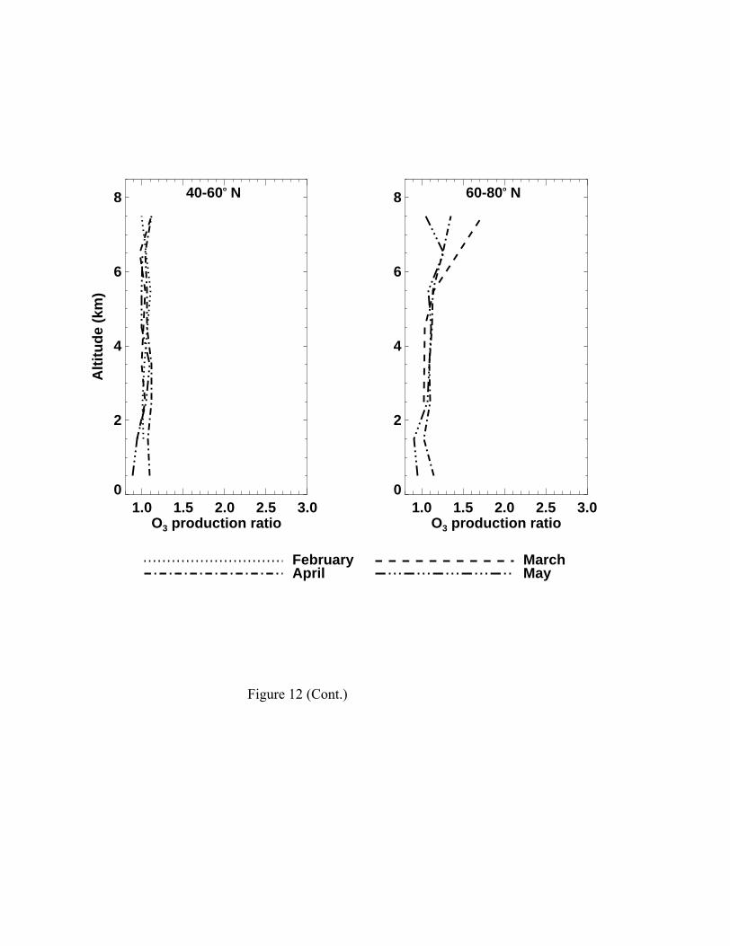
1.0 1.5 2.0 2.5 3.0O3 production ratio

0

2

4

6

8

Alt

itu

de

(km

)

40-60o N

1.0 1.5 2.0 2.5 3.0O3 production ratio

0

2

4

6

8 60-80o N

Figure 12 (Cont.)

February MarchApril May

0 20 40 60 80 1000

2

4

6

8A

ltit

ud

e (k

m)

40-60o N

Feb

0 20 40 60 80 1000

2

4

6

860-80o N

0 20 40 60 80 1000

2

4

6

8

Alt

itu

de

(km

)

Mar

0 20 40 60 80 1000

2

4

6

8

0 20 40 60 80 1000

2

4

6

8

Alt

itu

de

(km

)

Apr

0 20 40 60 80 1000

2

4

6

8

0 20 40 60 80 100NO2 (pptv)

0

2

4

6

8

Alt

itu

de

(km

)

May

0 20 40 60 80 100NO2 (pptv)

0

2

4

6

8

Figure 13

1 10 100 1000NOx (pptv)

1

10

100

1000

10000P

rim

ary

HO

x p

rod

uct

ion

(p

ptv

/day

)

0.030.06

0.1 0.10.06 0.1 0.10.06 0.1 0.20.07 0.1 0.3 0.40.07 0.1 0.3 0.3

0.030.09 0.2 0.3 0.4 0.1 0.2 0.3 0.6 0.9 0.1 0.1 0.3 0.6 0.90.08 0.2 0.3 0.6 1. 1.0.06 0.1 0.3 0.6 1. 1.0.09 0.1 0.3 0.8 2. 1.

0.2 0.2 0.8 1. 2. 0.3 0.7 1. 3. 3. 0.3 0.7 1. 3. 4.

0.5 3. 6. 0.8 3.

1 10 100NO (pptv)

1

10

100

1000

10000

Pri

mar

y H

Ox

pro

du

ctio

n (

pp

tv/d

ay)

0.03 0.09 0.1 0.1

0.04 0.10.02 0.05 0.1 0.2

0.04 0.1 0.2 0.30.05 0.1 0.2 0.30.08 0.1 0.2 0.30.07 0.2 0.2 0.4 0.8 1. 2.0.07 0.1 0.3 0.3 0.8 1.0.08 0.1 0.3 0.4 0.7 1.

0.1 0.3 0.5 0.8 2.0.09 0.1 0.3 0.8 1. 2.

0.1 0.3 0.8 2. 3. 0.4 1. 2. 4.

0.2 0.5 1. 2. 4. 0.3 1. 5.

0.9 2.

Figure 14

0 200 400 600 800NOy (pptv)

0

2

4

6

8A

ltit

ud

e (k

m)

40-60o N

0 200 400 600 800NOy (pptv)

0

2

4

6

8 60-80o N

0 100 200 300 400PAN (pptv)

0

2

4

6

8

Alt

itu

de

(km

)

0 100 200 300 400PAN (pptv)

0

2

4

6

8

Figure 15

-200 -100 0 100 200DNOy (pptv)

0

2

4

6

8

Alt

itu

de

(km

)

40-60o N

-200 -100 0 100 200DNOy (pptv)

0

2

4

6

8 60-80o N

Figure 15 (Cont.)

February MarchApril May

-10 0 10 20 30 40 50HNO3 P-L (pptv/day)

0

2

4

6

8A

ltit

ud

e (k

m)

40-60o N

-10 0 10 20 30 40 50HNO3 P-L (pptv/day)

0

2

4

6

8 60-80o N

-1 0 1 2 3 4 5PAN P-L (pptv/day)

0

2

4

6

8

Alt

itu

de

(km

)

-1 0 1 2 3 4 5PAN P-L (pptv/day)

0

2

4

6

8

Figure 16

February MarchApril May

0 1 2 3 4O3 P & L rates (ppbv/day)

0

2

4

6

8A

ltit

ud

e (k

m)

Production

Loss

Feb 40-60o N

0 1 2 3 4O3 P & L rates (ppbv/day)

0

2

4

6

8 Mar 40-60o N

0 1 2 3 4O3 P & L rates (ppbv/day)

0

2

4

6

8

Alt

itu

de

(km

)

Apr 40-60o N

0 1 2 3 4O3 P & L rates (ppbv/day)

0

2

4

6

8 May 40-60o N

Figure 17

0 1 2 3 4O3 P & L rates (ppbv/day)

0

2

4

6

8A

ltit

ud

e (k

m)

Feb 60-80o N

0 1 2 3 4O3 P & L rates (ppbv/day)

0

2

4

6

8 Mar 60-80o N

0 1 2 3 4O3 P & L rates (ppbv/day)

0

2

4

6

8

Alt

itu

de

(km

)

Apr 60-80o N

0 1 2 3 4O3 P & L rates (ppbv/day)

0

2

4

6

8 May 60-80o N

Figure 17 (Cont.)

1 2 3 4O3 loss rate (ppbv/day)

0

2

4

6

8A

ltit

ud

e (k

m)

Total lossO(1D) + H2OO3 + HO2

O3 + OH

Feb 40-60o N

1 2 3 4O3 loss rate (ppbv/day)

0

2

4

6

8 Mar 40-60o N

1 2 3 4O3 loss rate (ppbv/day)

0

2

4

6

8

Alt

itu

de

(km

)

Apr 40-60o N

1 2 3 4O3 loss rate (ppbv/day)

0

2

4

6

8 May 40-60o N

Figure 18

0.5 1.0 1.5 2.0O3 loss rate (ppbv/day)

0

2

4

6

8A

ltit

ud

e (k

m)

Feb 60-80o N

0.5 1.0 1.5 2.0O3 loss rate (ppbv/day)

0

2

4

6

8 Mar 60-80o N

0.5 1.0 1.5 2.0O3 loss rate (ppbv/day)

0

2

4

6

8

Alt

itu

de

(km

)

Apr 60-80o N

0.5 1.0 1.5 2.0O3 loss rate (ppbv/day)

0

2

4

6

8 May 60-80o N

Figure 18 (Cont.)

65

Mid Latitude

Ozo

ne (p

pbv)

60 observation

"model" 55

50

45

Feb Mar Apr May

65

High latitude

60

Ozo

ne (p

pbv)

55

50

45

Feb Mar Apr May

Figure 19

66