Species abundance distributions: moving beyond single prediction

R E V I E W A N DS Y N T H E S I S Species abundance distributions: moving beyond

single prediction theories to integration within an

ecological framework

Brian J. McGill,1* Rampal S.

Etienne,2 John S. Gray,3 David

Alonso,4 Marti J. Anderson,5

Habtamu Kassa Benecha,2 Maria

Dornelas,6 Brian J. Enquist,7

Jessica L. Green,8 Fangliang He,9

Allen H. Hurlbert,10 Anne E.

Magurran,6 Pablo A.

Marquet,10,11,12 Brian A.

Maurer,13 Annette Ostling,4

Candan U. Soykan,14 Karl I.

Ugland3 and Ethan P. White7

Abstract

Species abundance distributions (SADs) follow one of ecology�s oldest and most

universal laws – every community shows a hollow curve or hyperbolic shape on a

histogram with many rare species and just a few common species. Here, we review

theoretical, empirical and statistical developments in the study of SADs. Several key

points emerge. (i) Literally dozens of models have been proposed to explain the hollow

curve. Unfortunately, very few models are ever rejected, primarily because few theories

make any predictions beyond the hollow-curve SAD itself. (ii) Interesting work has been

performed both empirically and theoretically, which goes beyond the hollow-curve

prediction to provide a rich variety of information about how SADs behave. These

include the study of SADs along environmental gradients and theories that integrate

SADs with other biodiversity patterns. Central to this body of work is an effort to move

beyond treating the SAD in isolation and to integrate the SAD into its ecological context

to enable making many predictions. (iii) Moving forward will entail understanding how

sampling and scale affect SADs and developing statistical tools for describing and

comparing SADs. We are optimistic that SADs can provide significant insights into basic

and applied ecological science.

Keywords

Environmental indicators, macroecology, scientific inference, species abundance

distributions.

Ecology Letters (2007) 10: 995–1015

1Department of Biology, McGill University, 1205 Ave Dr Pen-

field, Montreal, QC H3A 1B1, Canada2Community and Conservation Ecology Group, University of

Groningen, Haren, The Netherlands3Department of Biology, University of Oslo, Oslo, Norway4Department of Ecology and Evolutionary Biology, University

of Michigan, Ann Arbor, MI, USA5Department of Statistics, University of Auckland, Auckland,

New Zealand6Gatty Marine Laboratory, University of St Andrews, Fife,

Scotland7Department of Ecology and Evolutionary Biology, University

of Arizona, Tucson, AZ, USA8School of Natural Sciences, University of California Merced,

Merced, CA, USA9Department of Renewable Natural Resources, University of

Alberta, Edmonton, Alberta, Canada

10National Center for Ecological Analysis and Synthesis,

University of California Santa Barbara, Santa Barbara,

CA, USA11Center for Advanced Studies in Ecology & Biodiversity

(CASEB), Departamento de Ecologıa, Facultad de Ciencias

Biolıgicas, Pontificia Universidad Catolica de Chile, Alameda

340, Santiago, Chile12Instituto de Ecologıa y Biodiversidad (IEB), Departamento de

Ciencias Ecologicas. Facultad de Ciencias, Universidad de Chile.

Casilla 653, Santiago, Chile13Department of Fisheries and Wildlife, Michigan State

University, East Lansing, MI, USA14School of Life Sciences, Arizona State University, Tempe, AZ,

USA

*Correspondence: E-mail: [email protected]

Ecology Letters, (2007) 10: 995–1015 doi: 10.1111/j.1461-0248.2007.01094.x

� 2007 Blackwell Publishing Ltd/CNRS

I N T R O D U C T I O N

What is an SAD?

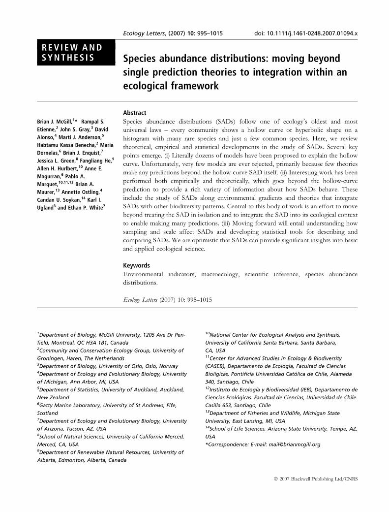
A species abundance distribution (SAD) is a description of

the abundance (number of individuals observed) for each

different species encountered within a community. As such,

it is one of the most basic descriptions of an ecological

community. When plotted as a histogram of number

(or percent) of species on the y-axis vs. abundance on an

arithmetic x-axis, the classic hyperbolic, �lazy J-curve� or

�hollow curve� is produced, indicating a few very abundant

species and many rare species (Fig. 1a). In this form, the law

appears to be universal; we know of no multispecies

community, ranging from the marine benthos to the

Amazonian rainforest, that violates it. When plotted in

other fashions, such as log-transforming the abundances

(Fig. 1b), more variability in shape occurs, giving rise to

considerable debate about the exact nature of SADs.

Nevertheless, the hollow-curve SAD on an arithmetic scale

is one of ecology�s true universal laws.

To be precise, we define an SAD as a vector of the

abundances of all species present in a community. Often,

the SAD is presented visually in a rank-abundance diagram

(RAD; Fig. 1c) where log-abundance is plotted on the y-axis

vs. rank on the x-axis. This plot contains exactly as much

information as the vector of abundances. In contrast,

histograms (Fig. 1a,b) involve binning and thus a loss of

information. In our definition, the term �community� is

vague (Fauth et al. 1996), and we do not choose to give a

precise definition here, but the choice becomes important

when we study the role of scale and sample size in SADs

(discussed later). The two most salient features of the SAD

are the fact that the species are not �labelled� by having a

species identity attached to the abundance and that zero

abundances are omitted. This loss of labels allows for

comparison of communities that have no species in

common, for example, a freshwater diatom community

and a tropical tree community. At the same time, SADs

enable nuanced questions and comparisons such as asking

which community has a higher proportion of rare species

Figure 1 Different ways to plot SADs. Abundance data for trees collected by Whittaker in the Siskiyou Mountains (Whittaker 1960) is

replotted here in three different formats. (a) A simple histogram of number of species vs. abundance on an arithmetic scale. A smoothed line

is added to highlight the overall shape. (b) A histogram with abundance on a log-scale. Note the traditional format is to use log2. (c) A rank-

abundance diagram (sometimes called a RAD). Log abundance (here log10 to make the reading of values easier) is plotted against the rank

(1 = highest abundance out to S = number of species for the lowest abundance). (d) An empirical cumulative distribution function (ECDF)

with a NLS logistic line fit through the data. Note that both the x- and y- axes are scaled into percentages. (e) A rank-abundance plot for data

from three different elevational bands showing different shapes observed. (f) The same three elevational bands now plotted as an ECDF.

Same colour ⁄ symbol legend as Fig. 1e.

996 B. J. McGill et al. Review and Synthesis


rather than just asking which community is more species

rich. In general, the SAD can be conceived of as falling in an

intermediate position on a spectrum of increasingly complex

descriptions of a community (Table 1).

Why are SADs important?

Not only is the hollow-curve SAD universal, but it is a

surprising, counterintuitive and therefore informative law.

Surely a prima facie null expectation is for abundances to be

more or less evenly distributed with some minor variation

because of body size, life history etc (i.e. normal with a mean

approximately equal to the number of individuals divided by

the number of species). In fact SADs are so uneven that this

null expectation is not even useful in studying SADs. Why?

If we can explain this high degree of unevenness, then we

likely will be in a position to make strong statements about

which mechanisms structure communities, be they species

interactions, random chance or some other factor. Thus

understanding SADs is a major stepping stone to under-

standing communities in general.

The raw data underlying an SAD (i.e. a census of the

number of individuals per species or even per morphospecies)

is among the most commonly collected data in ecology

(although SAD data is lacking for many types of communities

such as bacteria or mycorrhizae, and for larger organisms

complete censuses are empirically daunting to gather at even

intermediate spatial scales such as 50 ha). The overall

availability of data combined with the intermediate complex-

ity of SADs (Table 1), their potential for comparison among

disparate communities, and their visual nature have made

SADs very popular in ecological research. SADs are

commonly taught in undergraduate ecology and management

classes. The SAD is also pivotal in conservation – described as

the �science of scarcity� (Soule 1986); the relative terms

�common� and �rare� are given a clear definition in the context

of an SAD. In short, the SAD has played and is likely to

continue to play a central role in ecology.

Brief history

It is unclear exactly when ecologists first began to measure

SADs quantitatively. Yet the existence of a few very

common species and many very rare species was an obvious

fact even to casual observation. Audubon in the 1800s was

aware that birds in North America have abundances that

vary by as much as seven orders of magnitude (McGill 2006).

Darwin (1859) noted �Who can explain why one species

ranges widely and is very numerous, and why another allied

species has a narrow range and is rare? Yet these relations are

of the highest importance, for they determine the present

welfare and, as I believe, the future success and modification

Table 1 This table describes three common descriptions of community structure in increasing degrees of accuracy in parallel with decreasing

degrees of simplicity. Species abundance distributions are intermediate on these scales

Review and Synthesis Species abundance distributions 997


of every inhabitant of this world�. The first formally

published quantitative analysis of an SAD of which we are

aware is by Raunkiaer (1909) (although technically he

measured occupancy rather than abundance). By the 1940s

the use of histograms had become well-established (Fisher

et al. 1943; Preston 1948) and the use of a log-transformed

abundance (Preston 1948) was introduced. The RAD plot

was first introduced by MacArthur (1957). Note that the

empirical cumulative distribution (ECDF) is not often used,

but is mathematically equivalent to the RAD involving only a

swapping and rescaling of the axes. Fig. 1a–c shows the

three different ways these data are commonly plotted and

Fig. 1d shows the ECDF. Two reviews on SADs were

written in the 1960s and 1970s that implied we had worked

out the basic patterns and processes of SADs (Whittaker

1965; May 1975). But later reviews (Gray 1987; Marquet et al.

2003) express a belief that there has been a disappointing

lack of progress in the study of SADs.

We now provide more detail in the next three sections

covering, in order, theoretical, empirical and statistical

developments in the analysis of SADs. A healthy scientific

field will advance roughly in parallel in each of these three

areas. We conclude with a section identifying ways in which

SADs have failed to achieve parallel advancement in these

areas and suggest important directions to move forward.

T H E O R E T I C A L D E V E L O P M E N T S I N S A D S

Classical theoretical developments

The first theory attempting to explain the mechanism

underlying hollow-curve SADs was by Motomura (1932).

He pointed out that a sequential partition of a single niche

dimension by a constant fraction leads to the geometric

distribution. Fisher et al. (1943) argued for the logseries

distribution as the limit of a Poisson sampling process from

a gamma distribution (where the gamma was chosen only

because of its general nature). Kendall (1948a) put the

logseries on a more mechanistic footing by deriving it from

birth-death-immigration models. Preston (1948) argued for

a modified lognormal on the basis of the central limit

theorem. MacArthur (1957) built on Motomura�s idea of

partitioning a one-dimensional niche but used a random

stick-breaking process. This would seem to have set the

stage for a clear test with empirical data. Each theory made

distinct predictions: the geometric model predicts extremely

uneven abundances, broken stick predicts extremely even

abundances, while lognormal and logseries are intermediate

with distinct predictions about the proportions of very rare

species – high in logseries, low in lognormal. But an

empirical resolution has not occurred. With the possible

exception of the broken stick, none of the four classical

hypotheses have been eliminated. Instead, we have seen

literally dozens of new hypotheses added without elimina-

tion of older hypotheses.

Proliferation of models

Starting in the 1970s and running unabated to the present

day, mechanistic models (models attempting to explain the

causes of the hollow curve SAD) and alternative interpre-

tations and extensions of prior theories have proliferated to

an extraordinary degree (May 1975; Gray 1987; Tokeshi

1993; Marquet et al. 2003). Broadly speaking, we identify five

families of SAD models with over 40 members (see Table 2

for an incomplete list; see also Marquet et al. 2003 for a

similar analysis):

(1) Purely statistical: purely statistical theories take some

combination of the continuous gamma and lognormal

distributions with the discrete binomial, negative

binomial, and Poisson distributions. The lognormal

has many versions (see Table 2); we recommend using

either the simple, untruncated continuous lognormal

because of the extreme ease with which it is fit (mean

and standard deviation of log-transformed data) or the

Poisson lognormal because of its technical merits

(Bulmer 1974; Etienne & Olff 2005).

(2) Branching processes: when dealing with biological pro-

cesses, individuals are always derived from ancestor

individuals. This suggests a random-branching process

as a model.

(3) Population dynamics: a variety of population dynamic

models arrayed along a spectrum from purely deter-

ministic to purely stochastic can also produce realistic

SADs.

(4) Niche partitioning: another group of models is based on

dividing up a one-dimensional niche space. The oldest

SAD model is of this type (Motomura 1932).

(5) Spatial distribution: one can build spatial models of SADs

if one conceives of the SAD as counting all the

individuals falling within a particular region of space

and if one knows (or can model statistically): (i) the

spatial distribution of individuals within a species and

(ii) the distribution of species relative to each other.

Several of these families overlap. For example, neutral

models (Caswell 1976; Bell 2000; Hubbell 2001) are

stochastic population dynamic models but also branching

process models (Etienne & Olff 2004b), and the lognormal

can be the limit of population dynamics (Engen & Lande

1996b) or niche partitioning (Bulmer 1974; Sugihara 1980).

Major theoretical controversies

Given the proliferation of theories there has been

considerable debate (e.g. Alonso et al. 2006; Nekola &



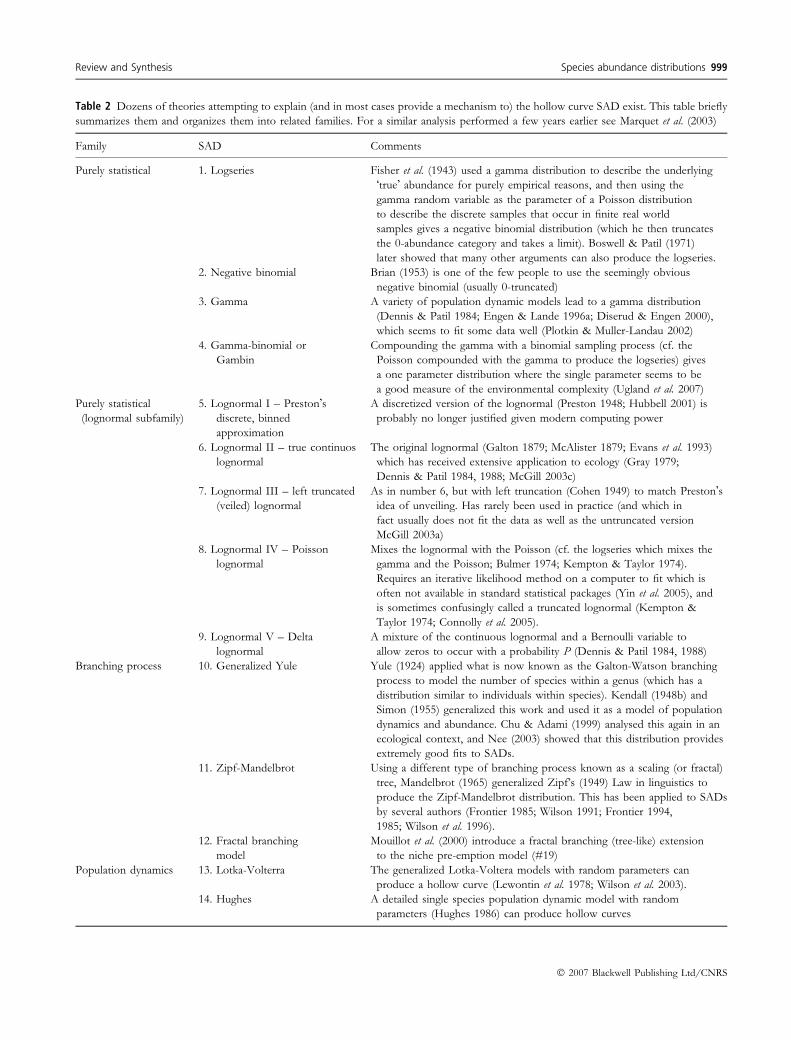
Table 2 Dozens of theories attempting to explain (and in most cases provide a mechanism to) the hollow curve SAD exist. This table briefly

summarizes them and organizes them into related families. For a similar analysis performed a few years earlier see Marquet et al. (2003)

Family SAD Comments

Purely statistical 1. Logseries Fisher et al. (1943) used a gamma distribution to describe the underlying

�true� abundance for purely empirical reasons, and then using the

gamma random variable as the parameter of a Poisson distribution

to describe the discrete samples that occur in finite real world

samples gives a negative binomial distribution (which he then truncates

the 0-abundance category and takes a limit). Boswell & Patil (1971)

later showed that many other arguments can also produce the logseries.

2. Negative binomial Brian (1953) is one of the few people to use the seemingly obvious

negative binomial (usually 0-truncated)

3. Gamma A variety of population dynamic models lead to a gamma distribution

(Dennis & Patil 1984; Engen & Lande 1996a; Diserud & Engen 2000),

which seems to fit some data well (Plotkin & Muller-Landau 2002)

4. Gamma-binomial or

Gambin

Compounding the gamma with a binomial sampling process (cf. the

Poisson compounded with the gamma to produce the logseries) gives

a one parameter distribution where the single parameter seems to be

a good measure of the environmental complexity (Ugland et al. 2007)

Purely statistical

(lognormal subfamily)

5. Lognormal I – Preston�sdiscrete, binned

approximation

A discretized version of the lognormal (Preston 1948; Hubbell 2001) is

probably no longer justified given modern computing power

6. Lognormal II – true continuos

lognormal

The original lognormal (Galton 1879; McAlister 1879; Evans et al. 1993)

which has received extensive application to ecology (Gray 1979;

Dennis & Patil 1984, 1988; McGill 2003c)

7. Lognormal III – left truncated

(veiled) lognormal

As in number 6, but with left truncation (Cohen 1949) to match Preston�sidea of unveiling. Has rarely been used in practice (and which in

fact usually does not fit the data as well as the untruncated version

McGill 2003a)

8. Lognormal IV – Poisson

lognormal

Mixes the lognormal with the Poisson (cf. the logseries which mixes the

gamma and the Poisson; Bulmer 1974; Kempton & Taylor 1974).

Requires an iterative likelihood method on a computer to fit which is

often not available in standard statistical packages (Yin et al. 2005), and

is sometimes confusingly called a truncated lognormal (Kempton &

Taylor 1974; Connolly et al. 2005).

9. Lognormal V – Delta

lognormal

A mixture of the continuous lognormal and a Bernoulli variable to

allow zeros to occur with a probability P (Dennis & Patil 1984, 1988)

Branching process 10. Generalized Yule Yule (1924) applied what is now known as the Galton-Watson branching

process to model the number of species within a genus (which has a

distribution similar to individuals within species). Kendall (1948b) and

Simon (1955) generalized this work and used it as a model of population

dynamics and abundance. Chu & Adami (1999) analysed this again in an

ecological context, and Nee (2003) showed that this distribution provides

extremely good fits to SADs.

11. Zipf-Mandelbrot Using a different type of branching process known as a scaling (or fractal)

tree, Mandelbrot (1965) generalized Zipf’s (1949) Law in linguistics to

produce the Zipf-Mandelbrot distribution. This has been applied to SADs

by several authors (Frontier 1985; Wilson 1991; Frontier 1994,

1985; Wilson et al. 1996).

12. Fractal branching

model

Mouillot et al. (2000) introduce a fractal branching (tree-like) extension

to the niche pre-emption model (#19)

Population dynamics 13. Lotka-Volterra The generalized Lotka-Voltera models with random parameters can

produce a hollow curve (Lewontin et al. 1978; Wilson et al. 2003).

14. Hughes A detailed single species population dynamic model with random

parameters (Hughes 1986) can produce hollow curves



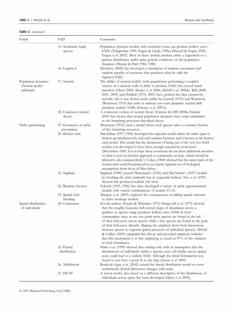
Table 2 (continued )

Family SAD Comments

15. Stochastic single

species

Population dynamic models with stochastic noise can produce hollow curve

SADs (Tuljapurkar 1990; Engen & Lande 1996a; Diserud & Engen 2000;

Engen et al. 2002). Most of these models produce either a lognormal or a

gamma distribution under quite general conditions on the population

dynamics (Dennis & Patil 1984, 1988)

16. Logistic-J Dewdney (2000) has developed a simulation of random encounters and

random transfer of resources that produces what he calls the

logistic-J SAD.

Population dynamics

(Neutral model

subfamily)

17. Neutral The ability of neutral models (with populations performing a coupled

version of a random walk or drift) to produce SADs has excited much

attention (Chave 2004; Alonso et al. 2006; McGill et al. 2006b). Bell (2000,

2001, 2003) and Hubbell (1979, 2001) have pushed this idea extensively

recently, but it was shown much earlier by Caswell (1976) and Watterson

(Watterson 1974) that with or without zero-sum dynamics neutral drift

produces realistic SADs (Etienne et al. 2007a).

18. Coalescent neutral

theory

A coalescent version of neutral theory (Etienne & Olff 2004b; Etienne

2005) has shown that neutral population dynamics have some similarities

to the branching processes described above.

Niche partitioning 19. Geometric or niche

preemption

Motomura (1932) used a model where each species takes a constant fraction

of the remaining resources.

20. Broken stick MacArthur (1957, 1960) developed the opposite model where the niche space is

broken up simultaneously and with random fractions and is known as the broken

stick model. This model has the distinction of being one of the very few SAD

models ever developed to have been strongly rejected by its inventor

(MacArthur 1966; �Let us hope these comments do not draw additional attention

to what is now an obsolete approach to community ecology, which should be

allowed to die a natural death.�). Cohen (1968) showed that the same math of the

broken stick could be produced by an exactly opposite set of biological

assumptions from those of MacArthur.

21. Sugihara Sugihara (1980) crossed Motomura�s (1932) and MacArthur�s (1957) models

by breaking the stick randomly but in sequential fashion. Nee et al. (1991)

showed this produced realistic left skew.

22. Random fraction Tokeshi (1993, 1996) has since developed a variety of niche apportionment

models with various combinations of models 19–21.

23. Spatial stick

breaking

Marquet et al. (2003) explored the consequences of adding spatial structure

to niche breakage models.

Spatial distribution

of individuals

24. Continuum Several authors (Gauch & Whittaker 1972; Hengeveld et al. 1979) showed

that the roughly Gaussian bell-curved shape of abundance across a

gradient or species range produces hollow curve SADs in local

communities since at any one point most species are found in the tail

of their bell-curve across species while a few species are found in the peak

of their bell-curve (thereby flipping the emphasis from local interactions

between species to regional spatial processes of individual species). McGill

& Collins (2003) expanded this theory and provided empirical evidence

that this mechanism is in fact explaining as much as 87% of the variation

in local abundances.

25. Fractal

distribution

Harte et al. (1999) showed that starting only with an assumption that the

distributions of individuals within a species were self-similar across spatial

scale could lead to a realistic SAD. Although the initial formulation was

found to not have a good fit to the data (Green et al. 2003)

26. Multifractal Borda-de-Agua et al. (2002) extend the fractal distribution model to cover

multifractals (fractal dimension changes with scale)

27. HEAP A newer model, also based on a different description of the distribution of

individuals across space has been developed (Harte et al. 2005).



Brown 2007) over whether some of the several dozen

models listed in Table 2 are �better� types of models a

priori than other models (independent of how well they fit

the data). This is of course a normative statement, which

depends heavily on one�s criteria for judging models. And

there are many possible criteria. Some of the

non-empirical criteria for favouring one theory over

another that have been invoked in the context of SADs

include:

(1) Many favour more mechanistic theories (usually the

statistical models are considered non-mechanistic), but

there is debate about what constitutes a mechanism.

Some consider neutral models that are derived from

basic principles of population dynamics more mecha-

nistic while others consider the niche partitioning

models that are a bit more abstract and static, yet based

on more �realistic� biological assumptions to be more

mechanistic.

(2) In a purely predictive paradigm (Peters 1991), predictive

success takes priority over mechanism.

(3) Others prefer parsimony (Ockham 1495) and related

issues of elegance and having few parameters.

(4) Some models develop or use extensive mathematical

machinery that allow for many different predictions to be

derived (such as the neutral models and the spatial

distribution models).

(5) Some models have parameters that can be easily estimated

independent of the SAD data one is trying to fit. In

principle neutral theory can do this, but in practice this

has not been performed successfully for neutral theory

(Enquist et al. 2002; Ricklefs 2003; McGill et al. 2006b)

or any other SAD model to our knowledge.

(6) The models also invoke varying degrees of symmetry

among the species. Many consider requirements of

symmetry undesirable because of obvious differences

among species. The most extreme such assumption is

the �neutrality� assumption of neutral theory (Hubbell

2001). This symmetry has also been controversial in

the derivation of the lognormal using the central limit

theorem (CLT; May 1975; Pielou 1977; Ugland &

Gray 1982; McGill 2003a; Williamson & Gaston

2005). But, in fact, all SAD models constructed so far

necessarily make some assumption of symmetry or

exchangeability between species. For example, the

niche partitioning models treat all species as identical

except for a single factor leading to pre-emption

(often suggested to be order of arrival which is

stochastic and independent of any species property).

The resolution of this may lie in recognizing that there

are ecological asymmetries but that species started

from symmetric initial conditions and later evolved

asymmetries (distinct life histories, physiology, and

population dynamics) in evolutionary time (Hubbell

2006; Marks & Lechowicz 2006).

Ultimately, which model approach is �best� will depend on

the question at hand. Predicting the rate of shifts in rarity

over time would likely require a mechanistic model, perhaps

based on population dynamics, while just predicting the

proportion of rare species might be better served by a

simple, easy to estimate statistical model.

Causes of the proliferation

As just described, there is room for more than one type of

SAD model. However, we believe the main cause of the

extensive proliferation has more to do with a failure to

successfully test and reject theories with data. Successful

branches of science use strong inference (Platt 1964) –

within a general model category, theories face off against

each other and the data pick a winner. The loser disappears

to science�s dustbin while the winning theory may then be

refined through additional iterations. The ever increasing

supply of new SAD theories without the rejection of any old

theories is the diametric opposite of what Platt (1964)

suggested and must be counted as a collective scientific

failure. The central problem has been that while most

theories make one and only one prediction – that SADs will

be a hollow-curve, predicting a hollow curve alone cannot

possibly be the basis of a decisive test between competing

theories because all the theories make this prediction. In

precise mathematical terms, SADs are �necessary� but not

�sufficient� for testing mechanistic theories. Any theory that

produces an SAD which is not a realistic hollow curve SAD

must surely be rejected (e.g. Etienne et al. 2007b), but having

a theory that produces a realistic hollow curve (even one

that closely fits some empirical data set) is not sufficient to

strongly support the theory. Further discussion on why

SADs have failed to lead to strong inference can be found in

Textbox 1 and in McGill (2003a) and Magurran (2005).

Historically, ecologists hoped that predicting subtle vari-

ations in the hollow curve would produce a decisive test. But

this has not worked well. Robert H. Whittaker (1975) noted

that �the study of (SADs) has not produced the single

mathematical choice … that the early work suggested might

be possible� which was echoed by Gray (1987). This is in part

because most attempts to evaluate SAD models have not been

sufficiently rigorous. We believe that at a minimum, attempts

to establish the superiority of a theoretically predicted SAD

must pay careful attention to points 1, 3, 4, and 5 in Textbox 1.

Specifically rigorous tests must compare multiple models

(point 1) using multiple measures of goodness of fit (point 4)

on multiple data sets (point 5). If one SAD theory emerges as

clearly superior (point 3), then – perhaps – there is some

justification for feeling a conclusion has been reached (but not



T E X T B O X 1 : K E Y C O M P O N E N T S O F S T R O N G

I N F E R E N C E I N S A D S

Progress in a scientific field depends on using a

successful inferential framework (Platt 1964). Here we

highlight six important inferential issues of high rele-

vance to making progress in the study of SADs.

(1) Competition: A disappointing number of presentations

of new SAD theories make no attempt to even

compare how well their predictions fit data in

comparison to other theories, thus avoiding even

the most basic requirement of Platt�s strong inference

or Burnham & Anderson�s (1998) model comparison

approach – a contest among theories. The end result

has been a large number of theories that fit reasonably

well without a clear sense of how the theories

compare with each other. When choosing models to

compare against, we strongly recommend including a

flexible, simple model like the untruncated lognormal.

Comparing against older but less flexible models such

as the logseries or geometric which are known to fail

to fit many datasets is weaker.

(2) Multiple mechanisms: Any given mathematical formu-

lation of an SAD can be created by many different

mechanisms, so fit to data cannot possibly be ultimate

proof of a particular mechanism (Pielou 1975; McGill

2003a). For example, Cohen (1968) showed that

multiple mechanisms lead to the broken stick,

Boswell & Patil (1971) showed that multiple mech-

anisms lead to the logseries while Ugland & Gray

(1983) showed that either niche-based competition or

neutrality can lead to neutral patterns and processes. It

is well known to philosophers of science that

similarity in pattern does not imply similarity in

process, but ecologists seem to frequently forget it.

This fact is clearly demonstrated by the recognition

that the SAD shape is an accurate description not only

of abundances within a community but of the

distribution of incomes among humans, the size of

storms, the frequency (abundance) of words in the

corpus of Shakespeare�s work (Nee 2003) and a host

of other distributions (McGill 2003a; Nekola &

Brown 2007). Either the mechanisms underlying this

one pattern must be extremely diverse or (perhaps

and) they must be extremely general and vague along

the lines of central limit theorems.

(3) Decisive weight of evidence: Most theories produce SADs

that are so similar to each other it is difficult to

distinguish them given the noisy data and the fact that

the differences are most pronounced in the tails which

are by definition infrequently observed (McGill

2003a,b; but see Etienne & Olff 2005). Indeed many

different SAD theories often fit a single dataset

extremely well (McGill 2003a,c) and to single one out

as best is to magnify minute differences. Does the

mere fact of one theory explaining 99.1% of the

variation make it better than the 2nd best theory

which explains 99.0%? This may seem like a contrived

example but it is quite realistic (McGill 2003c). Wilson

(1993) and Wilson et al. (1998) found that the noise of

sampling effect was so much larger than the small

differences that even when the SADs were Monte

Carlo generated from known theoretical distribu-

tions, the best fit model was usually a different one

than the model which generated the data.

(4) Robust measurement evidence: Different, inconsistent

methods are used. One data set (tropical trees on

Barro Colorado Island) has variously been claimed

to favour the neutral zero-sum multinomial or

lognormal depending on the methods used (McGill

2003c; Volkov et al. 2003). The outcome in this

particular case and in general is heavily dependent

on the measure of goodness of fit used (McGill

2003c; Magurran 2004; McGill et al. 2006b). Unfor-

tunately different goodness of fit measures all

emphasize different aspects of fit (chi-square on

log-binned data emphasizes fitting rare species,

calculating an r2 on the predicted vs. empirical

CDF emphasizes the abundances with the most

species - usually intermediate abundances, while

likelihood emphasizes avoidance of extreme out-

liers, etc.). It is common for different measures of fit

to select different SAD theories as providing the

best fit to a single data set (McGill 2003a). Thus any

claim of a superior fit must be robust by being

superior on multiple measures.

(5) General across multiple data sets: Even when consistent

methods are used, most theories will fit some

datasets well and other datasets poorly. Within the

basic hollow curve form there is great natural

variability in empirically observed shape (especially

for log-abundances) so it is almost always possible

to find a dataset for which a theory works and a

dataset for which it fails. One interpretation is that

different mechanisms are operating in different

communities and indeed this might be true for

fishes vs. trees (Etienne & Olff 2005). But is it really

parsimonious to believe that different processes

govern bird communities on different Breeding Bird

Survey routes within the same habitat type (McGill

2003a) or tropical trees on Barro Colorado island vs.

Pasoh forest (Volkov et al. 2003) based solely on

extremely small differences in the goodness of fit of

two different SAD theories?



about mechanism – point 2). But every study of which we are

aware that meets all (or even two) of these criteria has found

that no one SAD is superior (Wilson 1991; Wilson et al. 1996;

McGill 2003a; Volkov et al. 2003; Etienne & Olff 2005). We

do not believe that examining small variations in the nature of

the hollow curve will ever lead to strong inference and

decisive tests of SAD theories.

Integrating SADs with other patterns – towards a unifiedtheory?

One positive theoretical development in the study of SADs

is the demonstration that SADs are intimately linked in a

mathematical sense with a wide variety of other well-known

and novel macroecological patterns. This begins to

approach the rather grandiose goal of �unified theories�(Hanski & Gyllenberg 1997; Hubbell 2001; McGill 2003a;

Harte et al. 2005). These linkages can go in one of two

directions:

(a) One can start with only a hollow-curve SAD and then

derive other macroecological patterns from it, or.

(b) One can start with some set of assumptions and then

derive many macroecological patterns (including SADs)

from these assumptions.

Type (a) approaches are essentially elaborations of the

consequences of sampling from an uneven, hollow curve

SAD (see Textbox 2). Although many find this biologically

uninteresting, it is important to identify just how much is

explained by sampling from the hollow curve of the SAD

alone. For example, few people realize that Preston (1960)

showed that most of the species area relationship was well

explained by sampling from the logseries up to fairly large

spatial scales. From a testing point of view, it is also

important to realize that testing a prediction based on

sampling from an SAD (such as the species area curve

discussed in Textbox 2) is not really an independent

prediction from the hollow curve SAD prediction.

T E X T B O X 2 : S A D S – T H E M A S T E R P A T T E R N ?

If one starts with an SAD as the description of the relative

abundances of species in a community, one can start

sampling individuals from the SAD representation of the

community and derive a number of patterns. This makes

the SAD a central pattern in developing a unified theory

that links patterns together. Most directly, the species-

individual curve (SIC) which plots number of species as a

function of the number of individuals sampled follows

immediately. This curve is also known as a collector�scurve (Coleman 1981), a species accumulation curve

(Ugland et al. 2003) or a rarefaction curve (Sanders 1968).

The exact species-individual curve derived depends on the

exact SAD. For example, the logseries produces the exact

relation S = a ln(1 + N ⁄a) (Preston 1960; Williams

1964), neutral theory produces an alternative, more

complex formula (Etienne & Alonso 2005) while May

(1975) derived sampling formulas for several other SADs.

The analytical form of the SIC given an empirical SAD

(i.e. a sample with abundances of the different species

measured) is also well worked out (Simberloff 1972; Heck

et al. 1975; Olszewski 2004). It was recently shown

(Olszewski 2004) that the initial slope of the SIC is equal

to a common measure of community evenness, Hurlbert�s(1971) probability of interspecific encounter which is, in

turn, a bias-corrected form of Simpson�s diversity index.

Preston (1960) showed how the z-value of the species area

relationship (SAR) is entirely explained by passive

sampling from a logseries SAD at small scales with

another factor (presumably habitat heterogeneity) starting

to play a role only at larger scales (see also Williams 1964;

Rosindell & Cornell 2007). The SIC curve is often

conflated with a species area curve, but this is a good

equation only if the system is spatially homogeneous and

well-mixed. If dispersal limitation or environmental

heterogeneity exist, or equivalently there is spatial

autocorrelation or non-Poisson distribution of individuals

then the SAR curve will deviate from the SIC (Gotelli &

Colwell 2001; Olszewski 2004). He & Legendre (2002)

systematically explored how the SAR changes depending

on the degree of aggregation of individuals within species.

The pattern of nestedness (Atmar & Patterson 1993;

Wright et al. 1998), wherein the species occurring on

small patches are a proper subset of the species occurring

on larger patches can also be created entirely by a passive

sampling process from a hollow curve SAD – the species

found on all patches are the abundant species while the

species found only on the large patches are the rare

species (Connor & McCoy 1979; Fischer & Lindenmayer

2002). Similarly, sampling from an SAD can explain the

link between abundance and occupancy (Maurer 1990;

Lawton 1993; Gaston 1996; Gaston et al. 2000), leading

in turn to the derivation of the distribution of occupan-

cies (and hence range sizes by some definitions) from

SADs. Incidence curves (Hanski & Gyllenberg 1997) also

can be derived from passive sampling. These various

links to SADs can also be combined. For example, better

species accumulation (and species area) curves can be

achieved by taking the abundance ⁄ occupancy relation-

ship into account (He et al. 2002; Ugland et al. 2003). As

with the SAR, factors other than sampling from SADs

may also affect nestedness and abundance-occupancy,

but these are not yet well understood.



Type (b) approaches (the realization that a small set of

assumptions can simultaneously produce hollow curve

SADs and other macroecological patterns) are even more

recent and, we believe, promising. The most prominent

such example is neutral theory (Caswell 1976; Bell 2000,

2003; Hubbell 2001; Chave 2004), which can derive a great

many predictions including SADs but also the variability

over time of species abundances and true species area

curves (Rosindell & Cornell 2007) which incorporate the

role of dispersal limitation. To neutral theory�s great credit,

this is one reason it has been falsifiable (Dornelas et al.

2006; McGill et al. 2006b). In contrast most SAD models

such as the statistical and the niche partitioning models

make no prediction other than the hollow-curve SAD (but

see Ugland et al. 2007). This elegant ability of neutral

theory to produce many predictions is probably the main

reason for the interest and attention it has inspired (Alonso

et al. 2006).

Another body of work that has received less attention

but which can also derive many predictions focuses on the

spatial organization of individuals. An SAD is just a

collection of individuals in an area. If we can describe the

spatial distribution of individuals, then we can predict the

nature of the SAD for a given area using patterns (spatial

distribution) that may be closer to certain important

mechanisms such as dispersal and environmental hetero-

geneity. Empirically, we know the spatial distribution of

individuals within a species tends to be clumped (aggre-

gated; Condit et al. 2000) while the distribution between

species tends to be independent (spatial Poisson random-

ness; Hoagland & Collins 1997). Such distributions have

been studied at two very different scales. At very large

scales, this clumping has been described as an abundance

surface with an approximately Gaussian-bell curve shape

(Whittaker 1967; Brown et al. 1995), which leads to a

model producing a number of macroecological predictions

(Gauch & Whittaker 1972; Hengeveld et al. 1979; McGill &

Collins 2003). At smaller spatial scales the clumping of

individuals can be modelled based on fractals (Harte et al.

1999), statistical mechanics (Harte et al. 2005), or Ripley�sK-statistic (Plotkin & Muller-Landau 2002). At any scale

the two assumptions of independence between species and

aggregation within species lead to predictions about SADs

as well as a variety of other macroecological patterns

(Gauch & Whittaker 1972; Hengeveld & Haeck 1981;

McGill & Collins 2003; Harte et al. 2005). Such spatial

distribution models have also tended to lend themselves

well to empirical tests (Green et al. 2003; McGill & Collins

2003) .

In summary, there has been a proliferation of models

purporting to explain hollow-curve SADs. The vast majority

only predict the existence of a hollow-curve SAD, making

them essentially untestable. More recently, multifaceted

theories that link SADs with other patterns have emerged

and proven more amenable to testing.

E M P I R I C A L D E V E L O P M E N T O F S A D S

A healthy scientific discipline has theoretical development

and empirical discovery proceeding hand-in-hand. We

suggest that on the whole there has been more theoretical

development of SADs (Table 2) than empirical develop-

ment (or at least that theory has received more attention).

However, a great deal of interesting work has also occurred

in exploring empirical patterns of SADs. We will first

summarize the classical work on SADs found in ecology

textbooks, and then review a series of less-well-known,

intriguing but not strongly documented empirical results.

Classical empirical work

The bulk of the empirical work (and again the work put

into textbooks) has established two facts: (i) SADs follow

a hollow curve (on arithmetic scale) in every system

studied and (ii) Within this broad constraint, there is a

great deal of variation in the details, especially as

highlighted on a log-scale. We cannot possibly list every

empirical measurement of SADs as this is one of the

most common types of data collected in ecology. And in

all likelihood, the majority of such data sets have never

even been published (e.g. collected for management or

monitoring purposes). Hughes (1986) gives a compilation

of 222 different SADs and Dewdney (2000) gives a

compilation of 100. To our knowledge no SAD ever

measured violates the basic hollow-curve shape on an

arithmetic scale, justifying the claim that it is a universal

law. As with any pattern, it is possible that more work

will uncover an exception. For example, our knowledge

of the shape of SADs amongst taxa such as bacteria or

mycorrhizae is poor. But there is no debating that the

hollow-curve SAD is unusually general in nature.

At the same time enormous debate has gone into the

nature of the left side of SADs when plotted on a log-

abundance scale (Preston 1948; Hughes 1986; Southwood

1996; Hubbell 2001; McGill 2003b). Ecologists have

observed patterns ranging from a histogram that increases

to a mode in the middle (e.g. Fig. 2a BCI, BBS) through to

data that is largely flat until the middle abundances (e.g.

Fig. 2a Bass Strait) then on to data that has its mode at the

lowest abundance of N = 1 and decreases continuously

from there (e.g. Fig. 2a NCS). This goes back to the earliest

days, with Fisher suggesting that a lognormal was impossible

as his insect data showed the mode at the lowest abundance.

Preston explained this with the concept of a veil line

(Preston 1948). Preston�s veil line suggests that small

samples do not capture the truly rare species which causes



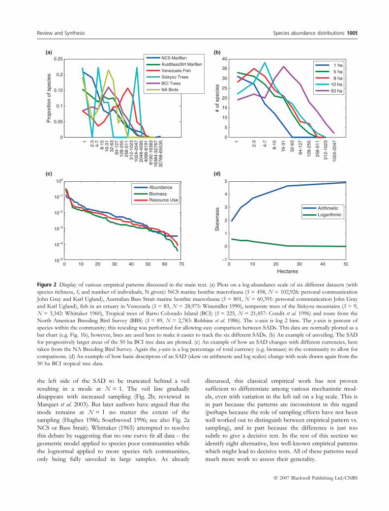
the left side of the SAD to be truncated behind a veil

resulting in a mode at N = 1. The veil line gradually

disappears with increased sampling (Fig. 2b; reviewed in

Marquet et al. 2003). But later authors have argued that the

mode remains at N = 1 no matter the extent of the

sampling (Hughes 1986; Southwood 1996; see also Fig. 2a

NCS or Bass Strait). Whittaker (1965) attempted to resolve

this debate by suggesting that no one curve fit all data – the

geometric model applied to species poor communities while

the lognormal applied to more species rich communities,

only being fully unveiled in large samples. As already

discussed, this classical empirical work has not proven

sufficient to differentiate among various mechanistic mod-

els, even with variation in the left tail on a log scale. This is

in part because the patterns are inconsistent in this regard

(perhaps because the role of sampling effects have not been

well worked out to distinguish between empirical pattern vs.

sampling), and in part because the difference is just too

subtle to give a decisive test. In the rest of this section we

identify eight alternative, less well-known empirical patterns

which might lead to decisive tests. All of these patterns need

much more work to assess their generality.

Figure 2 Display of various empirical patterns discussed in the main text. (a) Plots on a log-abundance scale of six different datasets (with

species richness, S, and number of individuals, N given): NCS marine benthic macrofauna (S = 458, N = 102,926: personal communication

John Gray and Karl Ugland), Australian Bass Strait marine benthic macrofauna (S = 801, N = 60,391: personal communication John Gray

and Karl Ugland), fish in an estuary in Venezuela (S = 83, N = 28,975: Winemiller 1990), temperate trees of the Siskyou mountains (S = 9,

N = 3,342: Whittaker 1960), Tropical trees of Barro Colorado Island (BCI) (S = 225, N = 21,457: Condit et al. 1996) and route from the

North American Breeding Bird Survey (BBS) (S = 89, N = 2,783: Robbins et al. 1986). The x-axis is log 2 bins. The y-axis is percent of

species within the community; this rescaling was performed for allowing easy comparison between SADs. This data are normally plotted as a

bar chart (e.g. Fig. 1b), however, lines are used here to make it easier to track the six different SADs. (b) An example of unveiling. The SAD

for progressively larger areas of the 50 ha BCI tree data are plotted. (c) An example of how an SAD changes with different currencies, here

taken from the NA Breeding Bird Survey. Again the y-axis is a log percentage of total currency (e.g. biomass) in the community to allow for

comparisons. (d) An example of how basic descriptors of an SAD (skew on arithmetic and log scales) change with scale drawn again from the

50 ha BCI tropical tree data.



Empirical pattern 1 – environmental gradient analysis

Community ecology is regaining interest in the environ-

mental (abiotic) context in which communities occur. In

particular, gradients of changing environment provide a

natural experiment or comparative basis for testing theories

about communities (McGill et al. 2006a) including SADs.

The 1970s saw a burst of analysis of SADs along gradients.

Fig. 1d gives an example; the data in Fig. 1d is from

Whittaker (1960) (inspired by a comparable plot with

different data in Whittaker 1965) that plots changes in SADs

along elevational gradients in productivity. Whittaker

interpreted the results as showing that low productivity

systems have extremely uneven SADs and are well fit by a

geometric SAD, while high productivity systems are well fit

by lognormal curves (and show the highest evenness). Later,

Whittaker (1975) repeated this analysis with a similar

outcome, but with the unique twist that he compared vastly

different communities (birds, trees, etc.). He thereby

illustrated one of our aforementioned advantages of SADs

– the ability to compare unrelated communities. Hubbell

(1979) likewise showed a similar plot along a latitudinal

productivity gradient, comparing different tree communities

ranging from boreal to tropical (again with little overlap in

species between communities compared). Thus a general

pattern of increasing evenness (more lognormal, less

geometric) with productivity was suggested. Unfortunately,

to our knowledge, this pattern seems to have had little

follow-up. It is also unclear how much this pattern was

driven solely by the change in species richness which has a

strong effect on the shape of RADs; better analytical

methods are needed. One study that did control for species

richness (Hurlbert 2004) confirmed that sites with greater

productivity had more species for a given number of

individuals and less dominance by the most abundant

species, indicating a positive productivity-evenness relation-

ship. Cotgreave & Harvey (1994) showed that more

complex habitats (often correlated with productivity)

showed SADs with higher evenness (they also showed that

communities with more similar body sizes showed less

evenness, suggesting a mechanism of competitive overlap

affecting SADs). Although the pattern of greater evenness

in high productivity environments is far from well docu-

mented, evidence to date is consistent; but we know of not

even one instance where a model for SADs attempted to

explain the change of SADs with productivity.

In the 1970s, marine ecologists began to explore whether

SADs might prove to be a good indicator of human-

disturbed (specifically polluted) environments. One of the

first such analyses (Gray 1979) explored various pollution

factors such as organic waste, oil and toxic industrial efflux

and found a decrease in rare species and an increase in

species of intermediate-abundance. Amazingly, of the 138

papers (as of March 2007) that cite this original work, one is

fresh water, six are terrestrial (mostly theoretical), and the

remaining 131 are all marine. Despite evidence that SAD

responses to human disturbance in marine systems apply

equally well to terrestrial taxa (Hill et al. 1995; Hamer et al.

1997) this tool remains almost unknown amongst terrestrial

practitioners, although Mouillot & Lepretre (2000) have also

found that SADs perform well in distinguishing terrestrial

communities under different influences and argue for their

use as indicators. The marine community has developed a

variety of elaborations on this basic idea such as k-

dominance plots (Patil & Taillie 1982; Lambshead et al.

1983) and abundance ⁄ biomass comparison (ABC) plots

(Warwick 1986; Clarke & Warwick 2001; Magurran 2004). It

seems that SADs have a high potential to serve as

environmental indicators, defined as an easily measured

index that is indicative of the state (�health�) of an ecosystem

(Bakkes 1994). While conservation uses indicators exten-

sively, the main challenge is to find ones that are easy to

measure but highly informative and usable with non-

technical audiences. SADs, which come from easily mea-

sured data and are intermediate in complexity, may have

tremendous potential.

Empirical pattern 2 – successional and other temporalgradients

Instead of comparing communities across space (gradients)

it is also possible to compare communities across time

(Magurran 2007). Bazzaz (1975) showed a series of SADs

along a successional gradient in old fields (with more

lognormal, more even communities occurring late in

succession just as for productivity). Caswell (1976) studied

changes in diversity over succession and found that his

version of neutral theory failed to produce empirically

observed patterns. This allowed Caswell to make a strong

(Plattian) inference about an SAD theory, supporting our

contention that this comparative approach holds promise.

Wilson et al. (1996) demonstrated fairly complex but

significant changes in which SAD fits the best over

succession in several grasslands, with evenness increasing.

Thibault et al. (2004) showed a significant directional change

in the shape of SADs over a 25 year period in a system

which was known to have experienced a strong climatic

trend (increased rainfall in their arid system).

Empirical pattern 3 – deconstruction or subsetting

Rather than comparing SADs from two communities, one

can compare SADs for two subsets within the same

community. This approach has been coined deconstruction

(Marquet et al. 2004). For example Labra et al. (2005) studied

a set of invasive bird species vs. a paired set of similar native



species and a random (unpaired) set of native species and

found that exotics showed a clear tendency towards higher

abundances, especially in the rare species (although they

pooled data from many sites making it not strictly an SAD).

The division of species into resident and transient also

shows very distinct differences in the shape of the SAD

(Magurran & Henderson 2003; Ulrich & Ollik 2004). On the

theoretical modelling side, a somewhat similar idea was

suggested by Etienne & Olff (2004a) who explored

constraints based on body mass between body size guilds,

but assumed neutrality within body size guilds. We know of

few other analyses, but imagine that deconstructions

comparing the SADs of species from different trophic

levels (e.g. predator vs. prey), ontogenetic stages (juvenile vs.

adult) or taxonomic groups (e.g. passerines vs. non-

passerines) might also prove interesting.

Empirical pattern 4 – transient species, scale and left-skew

Recent years have seen a rapid advance in understanding

what drives the shape of the left tail on a log scale, and in

particular the common observation that large scale data sets

are left-skewed (have more rare species). Gregory (2000)

showed that left skew on a log scale is common in large

(country-sized) assemblages of birds, but that it disappears

when species arguably not part of the community are

removed. Magurran & Henderson (2003) showed that

amongst fish in an estuary, the permanently resident species

were lognormal (with no excess of rare species), but the

transient species were logseries indicating a disproportionate

number of rare species. A similar result was obtained for

beetles (Ulrich & Ollik 2004). McGill (2003b) explored this

same idea in the context of autocorrelation. He showed low

autocorrelation (all transients) and high autocorrelation (few

transients) leads to zero skew, while intermediate autocor-

relation (mixture of residents and transients) leads to log-

left-skew (excess rare species) in both Monte Carlo models

and empirical data (see also Fig. 2d). Finally, neutral theory

(Hubbell 2001) predicts that higher rates of migration,

modelled by the parameter m, lead to more log-left skew.

Although immigration rates per se are hard to measure,

several authors (Hubbell 2001; Latimer et al. 2005) have fit

empirical data to the neutral theory and found more left-

skew (i.e. higher values of m) in cases where greater

immigration was expected. These independently developed

but intertwined lines of evidence point both empirically and

theoretically to the idea that communities more open to

immigration will have a higher proportion of rare species.

Empirical pattern 5 – multiple modes

It has occasionally been observed that SADs of large

assemblages appear to be multimodal, that is have more than

one peak in a histogram (Ugland & Gray 1982; Gray et al.

2005; see also Fig. 2a NA BBS Birds and Venezuelan Fish).

This is in contrast to most theories which have only a single

peak either at intermediate abundances (e.g. the lognormal) or

at N = 1 (e.g. logseries). Sampling noise and binning effects

can produce multiple peaks (as in Fig. 1a), but only small

ones, while peaks much larger than could be produced by

these effects are claimed to be observed. Preston�s method of

displaying SAD histograms on a log2 scale by dividing the

boundaries (1, 2, 4, etc) between adjacent bars has the effect

of smoothing out peaks that might actually occur at N = 1 or

N = 2 thereby hiding the potential for multiple peaks (Gray

et al. 2006). The existence and implications of multiple modes

in the SAD has been little explored. An analysis of 100

Breeding Bird Survey routes found that all 100 routes had a

peak at N = 1 or 2 and a second peak at higher numbers

(McGill unpublished data). One can use a finite mixture of

normal distributions on a log scale fit by expectation

maximization (MacLachlan & Peel 2000; Martinez & Marti-

nez 2002) combined with AIC or likelihood ratios to test for

the number of peaks. Using these methods, McGill (unpub-

lished data) analysed the 50 ha tropical tree plot at Barro

Colorado Island and found that AIC selected a model with

three peaks, just as predicted by Gray et al. (2005). In the

strongest evidence to date, Dornelas et al. (in preparation) not

only found multiple peaks but found that these peaks are

consistent as sample size increases (the peaks move to the

right as expected when sample size increases but the distance

between the peaks remains constant).

The exact number of peaks chosen will depend on one�spersonal preference in tradeoffs for parsimony vs. goodness

of fit (or the information criteria one chooses that makes these

tradeoffs for you). The fact that there is more than one peak in

the data for many communities suggests there is much to be

gleaned by documenting, testing, and explaining this pattern.

While the existence of multiple peaks on a log scale does not

reject the universal hollow curve law on an arithmetic scale, it

does reject every existing SAD theory which all produce

unimodal curves. One possibility is that these studies

inappropriately lumped together distinct guilds. If true then

deconstruction analysis might find appropriate separations

(Magurran & Henderson 2003; Marquet et al. 2004).

Empirical pattern 6 – High and low diversity systems

The vast majority of SADs have been studied in systems

with a moderate number of species (say 30–300). Recent

debate over SADs has relied extensively on a single data set:

the approximately 225 species, 50 ha tropical tree plot from

Barro Colorado Island. Yet patterns from extremely species

poor and extremely species rich systems do not necessarily

match generalizations derived from systems of intermediate

richness. For example, large swaths of boreal forest may



contain only half a dozen tree species. It is tempting to

ignore such systems as uninteresting, but they of course

represent large areas of the world�s surface and are of

considerable economic importance. Boreal forest SADs

tend to produce histograms that are quite flat (non-modal)

on a log-abundance histogram (or equivalently a straight line

on a RAD; e.g. see Fig. 2a Siskyou trees). These can be fit by

the geometric model (Motomura 1932). Models of SADs

generated by neutral theory or the lognormal actually fit

such data very poorly. Moreover, it is not uncommon in

few-species SADs for the two most abundant species to be

very similar in abundance (i.e. codominants; see the 1920–

2140 m band in Fig. 1e), which contradicts the geometric

model. At the other extreme, extraordinarily speciose

communities (100s of species amongst a few 1000s of

individuals) tend to produce an SAD that still looks

hyperbolic on a log-abundance scale (e.g. Fig. 2a NCS),

again fitting SAD models other than the logseries quite

poorly.

Empirical pattern 7 – measurement currencies other thanabundance

Ecologists have a long tradition of plotting histograms of

abundance, but plant ecologists sometimes use other

measures (e.g. percent cover) for reasons of convenience

and preference. It seems desirable to explore the implica-

tions of using different currencies to assess the importance

of a species (Tokeshi 1993; see Fig. 2c). Abundance is

clearly an important measure, but perhaps biomass, resource

use (roughly biomass to the � power; Savage et al. 2004) or

percent cover is more relevant (Chiarucci et al. 1999). More

importantly, perhaps one of these distributions can lead

more directly to a mechanistic theory. In particular, niche

partitioning models might be expected to more directly

explain resource use than abundance (Tokeshi 1993;

Thibault et al. 2004; Connolly et al. 2005; Ginzburg personal

communication). Ecologists studying marine systems have

long used differences in biomass and abundance plotted

together in curves called Abundance Biomass Comparisons

(ABC curves; Warwick 1986) as a diagnostic tool. Connolly

et al. (2005) showed that the effects of scale and the rate of

unveiling differ substantially between abundance and

biomass distributions. Thibault et al. (2004) also found that

the two curves showed very distinct patterns.

Empirical pattern 8 – Patterns based on �labelled� SADs

Our definition of SADs requires that the SAD be

�unlabelled�, but as we seek to advance our empirical

understanding of the patterns related to SADs, comparing

the abundance of individual species over time or space is

an obvious direction to turn (Dornelas et al. 2006; Etienne

2007). For example, how often does a rare species become

common or a common species become rare? Some

theories (Hanski 1982) predict fairly quick exchanges,

others (Hubbell 2001) predict fairly moderate rates of

change, while empirical data suggest that species retain

their basic status as common or rare up to one million

years (McGill et al. 2005). Wootton (2005) was able to

reject a particular SAD theory by experimentally removing

the dominant species and showing that the abundances of

the remaining species changed more than expected under

neutral theory. A similar result was obtained for frag-

mented tropical rainforests (Gilbert et al. 2006). Mac Nally

(2007) also shows greater difference in labelled than

unlabelled studies and introduces the �abundance spectrum�as a means of studying changes in labelled SADs. Murray

et al. (1999) has shown the potential of comparing labelled

SADS between sites.

A theory which not only predicts a hollow curve SAD but

predicts which species (or types of species) should be

abundant or rare would be extremely powerful. There has

been a great deal of speculation about which species should

be abundant (e.g. Rosenzweig & Lomolino 1997), but there

has been comparatively little success to date in the empirical

search for patterns (Murray et al. 1999, 2002). For example,

more common species tend to have smaller body size

(Damuth 1981, 1991; Marquet et al. 1990; White et al. 2007)

but the exact nature and strength of the relationship is still

debated (Russo et al. 2003; White et al. 2007). Careful

control for spatial variation and phylogeny may lead to

clearer results (Murray & Westoby 2000). Perhaps this is an

area where theory can produce new predictions to guide

empirical research. Recent work centred on traits may

provide such a solution (Shipley et al. 2006).

Finally, with labelled species we can look at questions

related to the phylogenetic context of the SAD (Webb et al.

2002). For example, how do the abundances of sister species

compare? A study by Sugihara et al. (2003) suggests that

sympatric, closely related species have reduced abundances,

presumably because of competition for more similar

resources than non-sister pairs.

In summary the classical empirical work on SADs clearly

established that the hollow-curve SAD is very general, but

that when placed on a log scale that magnifies the rarest

species considerable variation occurs. The classical work has

failed to strongly test and reject different mechanistic

theories. We identify eight patterns involving comparison of

SAD shape between communities or subsets of communi-

ties (pattern nos. 1–4), seeming exceptions (pattern nos.

5–6) and alternative views of SADs (pattern nos. 7–8) that

have promise for leading to stronger tests of mechanistic

models. Note that even the seeming exceptions (no. 5 and 6)

occur only on log-scales and do not violate the hollow-curve

rule on an arithmetic scale.



L I N K I N G T H E O R Y A N D D A T A – S T A T I S T I C A L

I S S U E S I N S A D S

Data and theory are tied together through a process of

measurement and quantification. In the case of SADs a

variety of statistical issues arise that may substantially affect

the appearance of the observed patterns and should be

resolved to ensure a tie between data and theory in which

we can have confidence. We identify four broad areas.

How does sampling affect the shape of SADs?

Every SAD is a finite sample, yet we know very little about

how much this affects the patterns we observe. Sampling

leads to variance. Variance means that SADs have error bars

around the curves that represent them. In a plot such as

Fig. 1d the lines appear distinct but it is hard to say without

error bars. We know little about how to place error bars and

do significance tests on SADs, and it is rarely performed.

Neutral theory has a sampling theory built in (Etienne 2005;

Etienne & Alonso 2005; Alonso et al. 2006), which is a

tremendous advantage, but this needs to be extended to

SADs more generally. Some basic machinery has been

developed (Pielou 1977; Dewdney 1998; McGill 2003b;

Green and Plotkin 2007), but much work remains. Munoz

et al. (in press) have shown that not only the variance but the

bias of neutral parameters derived from SADs can be

extremely high even when sample sizes are moderate (100s

of individuals; but see Etienne 2007). We cannot currently

answer several closely related basic questions of high

practical importance: what number of individuals ⁄ propor-

tion of individuals in a community ⁄ spatial extent do we

need to sample to have reasonable confidence that the SAD

obtained is a good approximation of the underlying

community? Is 1% of the individuals enough? or 1000 total

individuals?

How does scale affect the SAD?

Closely related to the question of sample size is the question

of scale. As one samples larger areas or for longer time

periods, the sample size increases, and issues of habitat

heterogeneity, b-diversity, clumping of individuals, and

autocorrelation must be addressed. It is entirely possible

that both the patterns and processes influencing the SAD

will change with scale (Wiens 1989; Levin 1992) as has been

found for other macroecological patterns (Rosenzweig

1995). For example, it has been the suggested that the shape

of an SAD changes with log left (negative) skew increasing

with scale possibly due to spatial autocorrelation (McGill

2003b; see Fig. 2d). Is there, then, a natural or optimal scale

at which to measure SADs? This returns to our original

definition of the SAD and the imprecision that is inherent in

measuring a poorly defined concept like �community�. Some

of the aforementioned links between SADs and other

macroecological theories may prove important.

How do we compare SADs?

Nearly all comparisons of SADs along gradients, decon-

structions or time trajectories to date have been purely by

visual inspection (Whittaker 1965; Hubbell 1979). Most

particularly, these visual inspections have been performed

on rank-abundance plots which, by using an x-axis that runs

from 1 to S (i.e. species richness), seriously confounds the

effects of species richness per se with other changes in the

shape of the SAD (e.g. lines appear quite distinct in Fig. 1d

but less so in Fig. 1f). Changes in species richness are a

legitimate factor that should be considered a change in

shape of the SAD. However, changes in richness so strongly

dominate in rank-abundance plots that no other changes are

easily considered. Is there any other change in the shape of

an SAD after controlling for the fact that productivity

affects richness? We cannot say at the present time (but see

Hurlbert 2004). It may be that the use of empirical

cumulative density function (ECDF) plots can remove

some of this bias (Fig. 1f). The analyses of human impact in

marine environments usually use such plots (Gray 1979) or

k-dominance plots (Lambshead et al. 1983) which are

another way to try to remove the effect of species richness.

Plots that use relative abundance (percent) of individuals or

percent of total species may help. Such methods represent

an improvement, but are still visual. More rigorous

multivariate methods are needed.

What kinds of variation are commonly found in SADs andhow are they related to each other?

We know almost nothing about the main axes of variation in

SADs. In morphometric analyses it is common to perform

some form of principal components analysis and have a few

orthogonal axes capture most of the variation. A similar

result has occurred in landscape ecology where over four

dozen landscape metrics were found to reduce to only six

distinct axes of variation (Riitters et al. 1995) capturing 87%

of the total variation. This needs to be performed for SADs.

Species richness, evenness and proportion of rare species

might well turn out to be distinct axes of variation, but at

the same time these factors may be correlated with each

other. Empirical results to date are mixed (Kempton &

Taylor 1974; Weiher & Keddy 1999; Stirling & Wilsey 2001;

Wilsey et al. 2005). What are the optimal indices that capture

the major axes of variation in SADs? We do not know. Two

recent developments are promising. The observation (Pueyo

2006) that the power distribution, logseries and lognormal

are all just successive terms in a Taylor series expansion



suggests that we may be able to develop a rigorous

framework for how flexible an SAD is needed in a particular

case (as well as giving some credence to the parameters of

these distributions as possibly being more general in

interpretation than currently believed). Secondly, a new

model, the gamma-binomial or gambin (Ugland et al. 2007),

seems to be able to fit a great many datasets well while

having only a single parameter that seems to do a good job

of discriminating along gradients.

G O I N G F O R W A R D

Like any field, the study of SADs has had successes and

failures. A major success is the frequent measurement of

SADs in a wide variety of taxa and geographic areas leading

to the establishment of the relative universality of the

hollow-curve SAD law. Another major success is uncover-

ing a variety of tantalizing possible empirical patterns that go

beyond the hollow-curve. A final success is that the SAD

has inspired a great deal of theoretical development in

community ecology. Against these successes must be

weighed several failures. These include not firmly establish-

ing any empirical patterns beyond the hollow curve and a

failure to develop tools to differentiate how much of the

patterns are due to sampling effects vs. other more

ecologically based effects. Probably the biggest shortcoming

to date has been the lack of strong inference wherein an

extreme proliferation of mechanistic models remains largely

untested.

How can we bring strong inference into the field of

SADs? Platt (1964) not only argues that we must bring

theories into competition with each other, which has

happened often enough in the study of SADs (Wilson

1991; Wilson et al. 1996; Etienne & Olff 2005), but the

theories must make distinct enough predictions that we can

have a decisive test. Similarly, Lakatos (1978) suggests that it

is the quality and novelty of predictions that make for a

successful research program. How do we move SAD

research to novel predictions leading to decisive tests?

We suggest that SADs, like most of ecology, will never

find the kinds of predictions that physics makes and which

Lakatos praised (such as the prediction of the existence of

Neptune from small perturbations in the position of

Uranus). Ecology does not make predictions that are

accurate to five decimal places like physics does. Instead,

Rosenzweig & Abramsky (1997) argues that not just SAD

theory but all of ecology does and should proceed by

�dipswitch testing� (for younger readers, a dipswitch is an

approximately 1 cm by 2 cm switching unit that contains

usually eight on ⁄ off switches on a printed circuit board that

used to be the main way to configure a computer). What

ecology does well is to make a lot of binary predictions

(y increases when x increases). A single binary prediction

that is empirically confirmed is weak evidence for a theory

(a priori 50 ⁄ 50 odds). But if, like a dipswitch, we have

enough binary predictions strung together, then it creates a

strong test that is achievable in ecology. This of course

assumes that the model making these multiple predictions is

parsimonious and not over-parameterized.

So where does the dipswitch of multiple predictions

emerge in the study of SADs? We believe that SADs are a

central pattern but cannot be an isolated pattern. We have

argued the greatest failing in the study of SADs is the

development of theories that make only a single prediction –

the hollow-curve shape. We advocate placing SADs into a

larger ecological context, such as the abiotic environment,

the trophic level in a food web, or the status as invasive

species. This will lead to many predictions resulting in

stronger testing and simultaneously demonstrate exactly

how centrally SADs are embedded in ecology as a whole.

These more integrated SADs are much more likely to

increase our understanding of the mechanisms that lead to

hollow-curve SADs. In a sign of the strength of these more

integrated approaches, it is possible to imagine controlled,

manipulative experiments (field or microcosm) that test

such integrated theories; heretofore SADs have depended

entirely on observational data. These ideas of integration

have been the main themes identified throughout the

theoretical, empirical and statistical sections of this

review. We summarize them into a top dozen list of

future directions for going forward in the study of SADs

(Textbox 3).

We are optimistic that the SAD will, in the long run,

prove to be one of the most important fundamental tools in

community ecology and management. But to get there we

must always think carefully about Platt�s model of strong

inference. We hope our proposed directions forward based

on producing more predictions by integrating SADs into

their ecological context and the many examples we gave of

work already following this direction will prove a catalyst.

Then maybe we will begin to answer the big questions in

SADs such as why are all SADs broadly similar (hollow

curve), where (and why) do predictable differences in the

finer-scale structure of SADs occur, and how might we best

quantify these differences?

A C K N O W L E D G E M E N T S

This manuscript is the product of a working group on �Tools

and fresh approaches for species abundance distributions�sponsored by the National Center for Ecological Analysis

and Synthesis. We thank Volker Bahn, Jonathan Chase,

Richard Feldman, Sarah Marx, Brad Murray, Julie Messier,

Genevieve Smith, Gerben Straatsma, Peter White and two

anonymous referees for helpful comments. We gratefully

acknowledge the funding and logistical support provided by



NCEAS. Various individual authors also gratefully

acknowledge individual support from NSF, NCEAS,

NSERC, NERC and other national funding agencies.

PAM acknowledges FONDAP 1501-1001 and FCM P05-

002.

R E F E R E N C E S

Alonso, D., Etienne, R.S. & McKane, A.J. (2006). The merits of

neutral theory. Trends Ecol. Evol., 21, 451–457.

Atmar, W. & Patterson, B.D. (1993). The measure of order and

disorder in the distribution of species in fragmented habitat.

Oecologia, 96, 373–382.

Bakkes, J.A. (1994). An Overview of Environmental Indicators: State of the

art and Perspectives. UNEP ⁄ Earthprint, Bilthaven, Netherlands.

Bazzaz, F.A. (1975). Plant species diversity in old-field successional

ecosystems in southern Illinois. Ecology, 56, 485–488.

Bell, G. (2000). The distribution of abundance in neutral com-

munities. Am. Nat., 155, 606–617.

Bell, G. (2001). Neutral macroecology. Science, 293, 2413–2418.

Bell, G. (2003). The interpretation of biological surveys. Proc. R Soc.

Lond. B, 270, 2531–2542.

Borda-de-Agua, L., Hubbell, S.P. & McAllister, M. (2002). Species-

area curves, diversity indices, and species abundance distribu-

tions: A multifractal analysis. Am. Nat., 159, 138–155.

Boswell, M.T. & Patil, G.P. (1971). Chance mechanisms generating

the logarithmic series distribution used in the analysis of number

of species and individuals. In: Statistical Ecology, Volume I, Spatial

Patterns and Statistical Distirbutions (eds Patil, G.P., Pielou, E.C. &

Waters, W.E.). Pennsylvania State University Press, University

Park, PA, pp. 99–130.

Brian, M.V. (1953). Species frequencies in random samples from

animal populations. J. Anim. Ecol., 22, 57–64.

Brown, J.H., Mehlman, D.H. & Stevens, G.C. (1995). Spatial var-

iation in abundance. Ecology, 76, 2028–2043.

Bulmer, M.G. (1974). Fitting poisson lognormal distribution to

species-abundance data. Biometrics, 30, 101–110.

Burnham, K.P. & Anderson, D.R. (1998). Model Selection and Mul-

timodel Inference: A Practical Information-Theoretic Approach. 2nd edn.

Springer, New York, NY.

Caswell, H. (1976). Community structure: a neutral model analysis.

Ecol. Monogr., 46, 327–354.

Chave, J. (2004). Neutral theory and community ecology. Ecol.

Lett., 7, 241–253.

Chiarucci, A., Wilson, J.B., Anderson, B.J. & De Dominicis, V.

(1999). Cover versus biomass as an estimate of species abundance:

does it make a difference to the conclusions? J. Veg. Sci., 10, 35–42.

Chu, J. & Adami, C. (1999). A simple explanation for taxon

abundance patterns. Int. Natl Acad. Sci., 96, 15017–15019.

Clarke, K.R. & Warwick, R.M. (2001). Change in Marine Communities:

An Approach to Statistical Analysis and Interpretation (PRIMER-E).

Plymouth Marine Laboratory, Plymouth, UK.

Cohen, A.C. (1949). On estimating the mean and standard devia-

tion of truncated normal distributions. J. Am. Stat. Assoc., 44,

518–525.

Cohen, J.E. (1968). Alternate derivations of a species-abundance

relation. Am. Nat., 102, 165.

Coleman, B. (1981). Random placement and species area relations.

Math. Biosci., 54, 191–215.

T E X T B O X 3 : T O P D O Z E N D I R E C T I O N S T O

P U R S U E I N S A D R E S E A R C H

For theoreticians:

(1) Produce theories that make many predictions simul-

taneously, of which a hollow curve SAD is only

one.

(2) Produce theories that attempt to predict some of the

patterns identified in our empirical section.

(3) Produce theories that incorporate questions about

sampling and scale discussed in our statistics

section.

(4) Explore exactly how much of and how many

macroecological patterns can be explained merely as a

result of sampling from a hollow-curve SAD.

(5) Test theories against other theories using multiple

datasets using multiple measures of goodness of fit.

For field ecologists:

(6) Collect additional data to confirm the patterns we

suggest might be general in our empirical section. In

particular collect data that is anchored in an

ecological context and along some axis of variation

(e.g. along gradients or containing deconstructable

sets such as data that spans across trophic levels).

(7) Collect SAD data in underrepresented systems such as

bacteria and extremely high or low diversity systems.

(8) Collect as large a sample size as possible. As described,

we do not know what a good sample size is, but it

clearly at least in the 100s and quite possibly in the

1000s of individuals. Similarly, clearly describe the

sample size, area and temporal duration of the

sample to make the data useful to others.

(9) Collect data using currencies in addition to abundance

such as biomass or resource use.

(10) Explore manipulative experiments (field and micro-

cosm) to test theories of SADs.

For statisticians:

(11) Develop a sampling theory of SADs to help under-

stand what variation is explainable by sampling.

Extend this theory to cover the effects of scale

(essentially autocorrelated sampling).

(12) Use multivariate statistics to develop a robust theory

of comparing SADs and identify the major indepen-

dent axes of variation in SADs.



Condit, R., Hubbell, S.P., LaFrankie, J.V., Sukumar, R., Manokaran,

N., Foster, R.B. et al. (1996). Species–area and species–individual

relationships for tropical trees: a comparison of three 50-ha

plots. J. Ecol., 84, 549–562.

Condit, R., Ashton, P.S., Baker, P., Bunyavejchewin, S., Guna-

tilleke, S., Gunatilleke, N. et al. (2000). Spatial patterns in the

distribution of tropical tree species. Science, 288, 1414–1418.

Connolly, S.R., Hughes, T.P., Bellwood, D.R. & Karlson, R.H.

(2005). Community structure of corals and reef fishes at multiple

scales. Science, 309, 1363–1365.

Connor, E.F. & McCoy, E.D. (1979). The statistics and biology of

the species–area relationship. Am. Nat., 113, 791–833.

Cotgreave, P. & Harvey, P.H. (1994). Evennes of abundance in

bird communities. J. Anim. Ecol., 63, 365–374.

Damuth, J. (1981). Population density and body size in mammals.

Nature, 290, 699–700.

Damuth, J. (1991). Of size and abundance. Nature, 351, 268–269.

Darwin, C. (1859). On the Origin of Species. Clows and Sons, London.

Dennis, B. & Patil, G.P. (1984). The gamma distribution and

weighted multimodal gamma distributions as models of popu-

lation abundance. Math. Biosci., 68, 187–212.

Dennis, B. & Patil, G.P. (1988). Applications in ecology. In:

Lognormal Distributions: Theory and Applications(edsCrow, E.L. &

Shimizu, K.). Marcel Dekker, New York, pp. 303–330.

Dewdney, A.K. (1998). A general theory of the sampling process

with applications to the �veil line�. Theor. Popul. Biol., 54, 294–302.

Dewdney, A.K. (2000). A dynamical model of communities and a

new species-abundance distribution. Biol. Bull., 198, 152–165.

Diserud, O.H. & Engen, S. (2000). A general and dynamic species

abundance model, embracing the lognormal and the gamma

models. Am. Nat., 155, 497–511.

Dornelas, M., Connolly, S.R. & Hughes, T.P. (2006). Coral reef

diversity refutes the neutral theory of biodiversity. Nature, 440,

80–82.

Engen, S. & Lande, R. (1996a). Population dynamic models gen-

erating species abundance distributions of the gamma type.

J. Theor. Biol., 178, 325–331.

Engen, S. & Lande, R. (1996b). Population dynamic models gen-

erating the lognormal species abundance distribution. Math.

Biosci., 132, 169–183.

Engen, S., Lande, R., Walla, T. & DeVries, P.J. (2002). Analyzing

spatial structure of communities using the two-dimensional

poisson lognormal species abundance model. Am. Nat., 160,

60–73.

Enquist, B.J., Sanderson, J. & Weiser, M.D. (2002). Modeling

macroscopic patterns in ecology. Science, 295, 1835–1837.

Etienne, R.S. (2005). A new sampling formula for neutral biodi-

versity. Ecol. Lett., 8, 253–260.

Etienne, R.S. (2007). A neutral sampling formula for multiple

samples and an �exact� test of neutrality. Ecol. Lett., 10, 608–618.

Etienne, R.S. & Alonso, D. (2005). A dispersal-limited sampling

theory for species and alleles. Ecol. Lett., 8, 1147–1156.

Etienne, R.S. & Olff, H. (2004a). How dispersal limitation shapes

species-body size distributions in local communities. Am. Nat.,

163, 69–83.

Etienne, R.S. & Olff, H. (2004b). A novel genealogical approach to

neutral biodiversity theory. Ecol. Lett., 7, 170–175.

Etienne, R.S. & Olff, H. (2005). Confronting different models of

community structure to species-abundance data: a Bayesian

model comparison. Ecol. Lett., 8, 493–504.

Etienne, R.S., Alonso, D. & McKane, A.J. (2007a). The zero-

sum assumption in neutral biodiversity theory. J. Theor. Biol.,

http://dx.doi.org/10.1016/j.jtbi.2007.06.010.

Etienne, R.S., Apol, M.E.F., Olff, H. & Weissing, F.J. (2007b).

Modes of speciation and the neutral theory of biodiversity.

Oikos, 116, 241–258.

Evans, M., Hastings, N. & Peacock, B. (1993). Statistical Distribu-

tions, 2nd edn. John Wiley & Sons, New York.

Fauth, J.E., Bernardo, J., Camara, M., Resetarits, W.J., Jr, Bus-

kirk, J.V. & McCollum, S.A. (1996). Simplifying the jargon of

community ecology: a conceptual approach. Am. Nat., 147,

282–286.

Fischer, J. & Lindenmayer, D.B. (2002). Treating the nestedness

temperature calculator as a �black box� can lead to false con-

clusions. Oikos, 99, 193–199.

Fisher, R.A., Corbet, A.S. & Williams, C.B. (1943). The relation

between the number of species and the number of individuals in

a random sample from an animal population. J. Anim. Ecol., 12,

42–58.

Frontier, S. (1994). Species-diversity as a fractal property of bio-

mass. In: Fractals in the Natural and Applied Sciences (ed. Novak, M.)

North-Holland Publishing, Amsterdam, pp. 119–127.

Frontier, S. (1985). Diversity and structure in aquatic ecosystems.

Oceanogr. Mar. Biol., 23, 253–312.

Galton, F. (1879). The geometric mean in vital and social statistics.

Proc. R Soc. Lond., 29, 365–367.

Gaston, K.J. (1996). The multiple forms of the interspecific

abundance-distribution relationship. Oikos, 76, 211–220.

Gaston, K.J., Blackburn, T.M., Greenwood, J.J.D., Gregory, R.D.,

Quinn, R.M. & Lawton, J.H. (2000). Abundance-occupancy

relationships. J. Appl. Ecol., 37, S39–S59.

Gauch, H.G.J. & Whittaker, R.H. (1972). Coencline simulation.

Ecology, 53, 446–451.

Gilbert, B., Laurance, W.F., Leigh, E.G., Jr & Nascimento, H.E.

(2006). Can neutral theory predict the responses of amazonian tree

communities to forest fragmentation? Am. Nat., 168, 304–317.

Gotelli, N.J. & Colwell, R.K. (2001). Quantifying biodiversity:

procedures and pitfalls in the measurement and comparison of

species richness. Ecol. Lett., 4, 379–391.

Gray, J.S. (1979). Pollution-induced changes in populations. Philos.

Trans. R Soc. Lond. B, 286, 545–561.

Gray, J.S. (1987). Species-abundance patterns. In: Organization of

Communities Past and Present (eds Gee, J.H.R. & Giller, P.S.).

Blackwell Science, Oxford, pp. 53–68.

Gray, J.S., Bjorgesaeter, A. & Ugland, K.I. (2005). The impact of

rare species on natural assemblages. J. Anim. Ecol., 74,

1131–1139.

Gray, J.S., Bjorgesaeter, A. & Ugland, K.I. (2006). On plotting

species abundance distributions. J. Anim. Ecol., 75, 752–756.

Green, J.L. & Plotkin, J.B. (2007). A statistical theory for sampling

species abundances. Ecol. Lett., 10, doi:10.1111/j.1461-0248.

2007.01101.x.

Green, J.L., Harte, J. & Ostling, A. (2003). Species richness,

endemism and abundance patterns: tests of two fractal models in

a serpentine grassland. Ecol. Lett., 6, 919–928.

Gregory, R.D. (2000). Abundance patterns of European breeding

birds. Ecography, 23, 201–208.

Hamer, K.C., Hill, J.K., Lace, L.A. & Langan, A.M. (1997). Eco-

logical and biogeographical effects of forest disturbance on

tropical butterflies of Sumba Indonesia. J. Biogeogr., 24, 67–75.



Hanski, I. (1982). Dynamics of regional distribution: the core and

satellite species hypothesis. Oikos, 38, 210–221.

Hanski, I. & Gyllenberg, M. (1997). Uniting two general patterns in

the distribution of species. Science, 275, 397–400.

Harte, J., Kinzig, A.P. & Green, J. (1999). Self-similarity in the

distribution and abundance of species. Science, 284, 334–336.

Harte, J., Conlisk, E., Ostling, A., Green, J.L. & Smith, A.B. (2005).

A theory of spatial structure in ecological communities at mul-

tiple spatial scales. Ecol. Monogr., 75, 179–197.

He, F.L. & Legendre, P. (2002). Species diversity patterns derived

from species–area models. Ecology, 83, 1185–1198.

He, F., Gaston, K.J. & Wu, J. (2002). On species occupancy-

abundance models. Ecoscience, 9, 119–126.

Heck, K.L.J., Van Belle, G. & Simberloff, D. (1975). Explicit

calculation of the rarefaction diversity measurement and the

determination of sufficient sample size. Ecology, 56, 1459–

1461.

Hengeveld, R. & Haeck, J. (1981). The distribution of abundance II

Models and implications. Proc. K. Ned. Akad. Wet. C, 84, 257–284.

Hengeveld, R., Kooijman, S.A.L.M. & Taillie, C. (1979). A spatial

model explaining species-abundance curves. In: Statistical Distri-

butions in Ecological Work (eds Ord, J.K., Patil, G.P. & Taillie, C.).

International Co-operative Publishing House, Fairland, MD,

pp. 337–347.

Hill, J.K., Hamer, K.C., Lace, L.A. & Banham, W.M.T. (1995).

Effects of selective logging on tropical forest butterflies on

Buru, Indonesia. J. Appl. Ecol., 32, 754–760.

Hoagland, B.W. & Collins, S.L. (1997). Gradient models, gradient

analysis, and hierarchical structure in plant communities. Oikos,

78, 23–30.

Hubbell, S.P. (1979). Tree dispersion, abundance and diversity in a

tropical dry forest. Science, 203, 1299–1309.

Hubbell, S.P. (2001). A Unified Theory of Biodiversity and Biogeography.

Princeton University Press, Princeton.

Hubbell, S.P. (2006). Neutral theory and the evolution of ecological

equivalence. Ecology, 87, 1387–1398.

Hughes, R.G. (1986). Theories and models of species abundance.

Am. Nat., 128, 879–899.

Hurlbert, S.H. (1971). The nonconcept of species diversity: a

critque and alternative parameters. Ecology, 52, 577–586.

Hurlbert, A.H. (2004). Species–energy relationships and habitat

complexity. Ecol. Lett., 7, 714–720.

Kempton, R.A. & Taylor, L.R. (1974). Log-series and log-normal

parameters as diversity discriminants for lepidoptera. J. Anim.

Ecol., 43, 381–399.

Kendall, D.G. (1948a). On some modes of population growth

leading to Fisher, R.A. logarithmic series distribution. Biometrika,

35, 6–15.

Kendall, D.G. (1948b). On the generalized �birth-and-death� pro-

cess. Ann. Math. Stat., 19, 1–15.

Labra, F.A., Abades, S. & Marquet, P.A. (2005). Distribution and

abundance: scaling patterns in exotic and native bird species.

In: Species Invasions. Insights Into Ecology, Evolution and Biogeography

(eds Sax, D.F., Stachowicz, J.J. & Gaines, S.D.). Sinauer Asso-

ciates, Sunderland, MA, pp. 421–446.

Lakatos, I. (1978). Introduction: science and pseudoscience. In: The

Methodology of Scientific Research Programs (eds Worrall, J. & Currie,

G.). Cambridge University Press, Cambridge, pp. 1–8.

Lambshead, P.J.D., Platt, H.M. & Shaw, K.M. (1983). The detec-

tion of differences among assemblages of marine benthic species

based on an assessment of dominance and diversity. J. Nat. His.,

17, 859–874.

Latimer, A.M., Silander, J.A. & Cowling, R.M. (2005). Neutral

ecological theory reveals isolation and rapid speciation in a

biodiversity hot spot. Science, 309, 1722–1725.

Lawton, J.H. (1993). Range, population abundance and conserva-

tion. Trends Ecol. Evol., 8, 409–413.

Levin, S.A. (1992). The problem of pattern and scale in ecology.

Ecology, 73, 1943–1967.

Lewontin, R.C., Ginzburg, L.R. & Tuljapurkar, S.D. (1978). Het-

erosis as an explanation for large amounts of genic polymor-

phism. Genetics, 88, 149–170.

Mac Nally, R. (2007). Use of the abundance spectrum and relative-

abundance distributions to analyze assemblage change in mas-

sively altered landscapes. Am. Nat., in press.

MacArthur, R. (1957). On the relative abundance of bird species.

Proc. Natl Acad. Sci., 43, 293–295.

MacArthur, R. (1960). On the relative abundance of species. Am.

Nat., 94, 25–36.

MacArthur, R. (1966). Note on Mrs Pielou�s comments. Ecology, 47,

1074.

MacLachlan, G. & Peel, D. (2000). Finite Mixture Models. John Wiley

& Sons, New York.

Magurran, A.E. (2004). Measuring Biological Diversity, 2nd edn.

Blackwell, Oxford.

Magurran, A.E. (2005). Species abundance distributions: pattern or

process? Funct. Ecol., 19, 177–181.

Magurran, A.E. (2007). Species abundance distributions over time.

Ecol. Lett., 10, 347–354.

Magurran, A.E. & Henderson, P.A. (2003). Explaining the excess

of rare species in natural species abundance distributions. Nature,

422, 714–716.

Mandelbrot, B. (1965). Information theory and psycholinguistics.

In: Scientific Psychology: Principles and Applications, (ednWolman,

B.A. & Nagel, E.N.). Basic Books, New York, pp. 350–368.

Marks, C.O. & Lechowicz, M.J. (2006). Alternative designs and the

evolution of functional diversity. Am. Nat., 167, 55–66.

Marquet, P.A., Navarrete, S.A. & Castilla, J.C. (1990). Scaling

population density to body size in rocky intertidal communities.

Science, 250, 1125–1127.

Marquet, P.A., Keymer, J.A. & Cofre, H. (2003). Breaking the

stick in space: of niche models, metacommunities and patterns

in the relative abundance of species. In: Macroecology: Concepts and

Consequences (eds Blackburn, T.M. & Gaston, K.J.). Blackwell

Science, Oxford, pp. 64–86.

Marquet, P.A., Fernandez, M., Navarrete, S.A. & Valdivinos, C.

(2004). Diversity emerging: towards a deconstruction of bio-

diversity patterns. In: Frontiers of Biogeography: New Directions in

the Geography of Nature (ed Heaney, M.L.a.L.R.). Cambridge

University Press, Cambridge, pp. 192–209.

Martinez, W.L. & Martinez, A.R. (2002). Computational Statistics

Handbook With MATLAB. Chapman & Hall ⁄ CRC, Boca Raton.

Maurer, B.A. (1990). The relationship between distribution and

abundance in a patchy environment. Oikos, 58, 181–189.

May, R.M. (1975). Patterns of species abundance and diversity. In:

Ecology and Evolution of Communities (eds Cody, M.L. & Diamond,

J.M.). Belknap Press of Harvard University Press, Cambridge

MA, pp. 81–120.

McAlister, D. (1879). The law of the geometric mean. Proc. R Soc.

Lond., 29, 367–376.



McGill, B. (2003a). Strong and weak tests of macroecological

theory. Oikos, 102, 679–685.

McGill, B.J. (2003b). Does Mother Nature really prefer rare species

or are log-left-skewed SADs a sampling artefact? Ecol. Lett., 6,

766–773.

McGill, B.J. (2003c). A test of the unified neutral theory of bio-

diversity. Nature, 422, 881–885.

McGill, B.J. (2006). A renaissance in the study of abundance. Sci-

ence, 314, 770–771.

McGill, B. & Collins, C. (2003). A unified theory for macroecology

based on spatial patterns of abundance. Evol. Ecol. Res., 5, 469–

492.

McGill, B.J., Hadly, E.A. & Maurer, B.A. (2005). Community

inertia of Quaternary small mammal assemblages in North

America. Proc. Natl Acad. Sci., 102, 16701–16706.

McGill, B.J., Enquist, B.J., Weiher, E. & Westoby, M. (2006a).

Rebuilding community ecology from functional traits. Trends

Ecol. Evol., 21, 178–185.

McGill, B.J., Maurer, B.A. & Weiser, M.D. (2006b). Empirical

evaluation of the neutral theory. Ecology, 87, 1411–1423.

Motomura, I. (1932). On the statistical treatment of communities.

Zool. Mag., 44, 379–383.

Mouillot, D. & Lepretre, A. (2000). Introduction of relative

abundance distribution (RAD) indices, estimated from the rank-

frequency diagrams (RFD), to assess changes in community

diversity. Environ. Monit. Assess., 63, 279–295.

Mouillot, D., Lepretre, A., Andrei-Ruiz, M.C. & Viale, D. (2000).

The Fractal model: a new model to describe the species accu-

mulation process and relative abundance distribution (RAD).

Oikos, 90, 333–342.

Munoz, F., Couteron, P., Ramesh, B. & Etienne, R. (2007).

Estimating parameters of neutral communities: from one single

large to several small samples. Ecology, (in press).

Murray, B.R. & Westoby, M. (2000). Properties of species in the tail

of rank-abundance curves: the potential for increase in abun-

dance. Evol. Ecol. Res., 2, 583–592.

Murray, B.R., Rice, B.L., Keith, D.A., Myerscough, P.J., Howell, J.,

Floyd, A.G. et al. (1999). Species in the tail of rank-abundance

curves. Ecology, 80, 1806–1816.

Murray, B.R., Thrall, P.H., Gill, A.M. & Nicotra, A.B. (2002). How

plant life-history and ecological traits relate to species rarity and

commonness at varying spatial scales. Aust. Ecol., 27, 291–310.

Nee, S. (2003). The unified phenomenological theory of biodi-

versity. In: Macroecology: Concepts and Consequences (eds Blackburn,

T.M. & Gaston, K.J.). Blackwell Science, Oxford, pp. 31–44.

Nee, S., Harvey, P.H. & May, R.M. (1991). Lifting the veil on

abundance patterns. Proc. R Soc Lond Ser. B Biol. Sci., 243, 161–163.

Nekola, J.C. & Brown, J.H. (2007). The wealth of species: eco-

logical communities, complex systems and the legacy of Frank

Preston. Ecol. Lett., 10, 188–196.

Ockham, W.. (1495). Quaestiones et decisiones in quattuor libros Senten-

tiarum Petri Lombardi Editioni Lugdenensi, i, dist. 27, qu. 2, K.

Olszewski, T.D. (2004). A unified mathematical framework for the

measurement of richness and evenness within and among

multiple communities. Oikos, 104, 377–387.

Patil, G.P. & Taillie, C. (1982). Diversity as a concept and its

measurement. J. Am. Stat. Assoc., 77, 548–561.

Peters, R.H. (1991). A Critique for Ecology. Cambridge University

Press, Cambridge.

Pielou, E.C. (1975). Ecological Diversity. John Wiley & Sons,

New York.

Pielou, E.C. (1977). Mathematical Ecology. John Wiley & Sons,

New York.

Platt, J.R. (1964). Strong inference. Science, 146, 347–353.

Plotkin, J.B. & Muller-Landau, H.C. (2002). Sampling the species

composition of a landscape. Ecology, 83, 3344–3356.

Preston, F.W. (1948). The commonness and rarity of species.

Ecology, 29, 254–283.

Preston, F.W. (1960). Time and space and the variation of species.

Ecology, 41, 611–627.

Pueyo, S. (2006). Diversity: between neutrality and structure. Oikos,

112, 392–405.

Raunkiaer, C. (1909). Formationsundersogelse og Formationsstat-

istik. Bot. Tidskr., 30, 20–132.

Ricklefs, R.E. (2003). A comment on Hubbell�s zero-sum ecolog-

ical drift model. Oikos, 100, 185–192.

Riitters, K.H., O�Neill, R.V., Hunsaker, C.T., Wickham, J.D.,

Yankee, D.H., Timmins, S.P. et al. (1995). A factor analysis of

landscape pattern and structure metrics. Landsc. Ecol., 10, 23–

39.

Robbins, C.S., Bystrak, D. & Geissler, P.H. (1986). The Breeding Bird

Survey: Its First Fifteen Years, 1965–1979. US Department of the

Interior Fish and Wildlife Service, Washington, DC.

Rosenzweig, M.L. (1995). Species Diversity in Space and Time. Cam-

bridge University Press, Cambridge.

Rosenzweig, M.L. & Abramsky, Z. (1997). Two gerbils of the

Negev: a long-term investigation of optimal habitat selection and

its consequences. Evol. Ecol., 11, 733–756.

Rosenzweig, M.L. & Lomolino, M.V. (1997). Who gets the short

bits of the broken stick. In: The Biology of Rarity: Causes and

Consequences of Rare-Common Differences (eds Kunin, W.E. &

Gaston, K.J.). Chapman & Hall, London, pp. 63–90.

Rosindell, J. & Cornell, S.J. (2007). Species-area relationships from

a spatially explicit neutral model in an infinite landscape. Ecol.

Lett., 7, 586–595.

Russo, S.E., Robinson, S.K. & Terborgh, J. (2003). Size-abundance

relationships in an amazonian bird community: implications for

the energetic equivalence rule. Am. Nat, 161, 267–283.

Sanders, H.L. (1968). Marine benthic diversity: a comparative

study. Am. Nat., 102, 243–282.

Savage, V.M., Gillooly, J.F., Brown, J.H., West, G.B. & Charnov,

E.L. (2004). Effects of body size and temperature on population

growth. Am. Nat., 163, 429–441.

Shipley, B., Vile, D. & Garnier, E. (2006). From plant traits to plant

communities: a statistical mechanistic approach to biodiversity.

Science, 314, 812–814.

Simberloff, D.S. (1972). Properties of the rarefaction diversity

measurement. Am. Nat., 106, 414–418.

Simon, H.A. (1955). On a class of skew distribution functions.

Biometrika, 42, 425–440.

Soule, M.E. (1986). Conservation Biology: The Science of Scarcity and

Diversity. Sinauer Associates, Sunderland, MA.

Southwood, T.R.E. (1996). The Croonian lecture, 1995: natural

communities: structure and dynamics. Philos. Trans. Biol. Sci., 351,

1113–1129.

Stirling, G. & Wilsey, B. (2001). Empirical relationships between

species richness, evenness, and proportional diversity. Am. Nat.,

158, 286–299.



Sugihara, G. (1980). Minimal community structure: an explanation

of species-abundance patterns. Am. Nat., 116, 770–787.

Sugihara, G., Bersier, L.F., Southwood, T.R.E., Pimm, S.L. & May,

R.M. (2003). Predicted correspondence between species abun-

dances and dendrograms of niche similarities. Proc. Natl Acad. Sci.

USA., 100, 5246–5251.

Thibault, K.M., White, E.P. & Ernest, S.K.M. (2004). Temporal

dynamics in the structure and composition of a desert rodent

community. Ecology, 85, 2649–2655.

Tokeshi, M. (1993). Species abundance patterns and community

structure. Adv. Ecol. Res., 24, 111–186.

Tokeshi, M. (1996). Power fraction: a new explanation of relative

abundance patterns in species-rich assemblages. Oikos, 75,

543–550.

Tuljapurkar, S.D. (1990). Population Dynamics in Variable Environ-

ments. Springer-Verlag, New York.

Ugland, K.I. & Gray, J.S. (1982). Lognormal distributions and the

concept of community equilibrium. Oikos, 39, 171–178.

Ugland, K.I. & Gray, J.S. (1983). Reanalysis of Caswell�s neutral

models. Ecology, 64, 603–605.

Ugland, K.I., Gray, J.S. & Ellingsen, K.E. (2003). The species-

accumulation curve and estimation of species richness. J. Anim.

Ecol., 72, 888–897.

Ugland, K.I., Lambshead, P.J.D., McGill, B., Gray, J.S., O�Dea, N.,

Ladle, R.J. et al. (2007). Modelling dimensionality in species

abundance distributions: description and evaluation of the

Gambin model. Evol. Ecol. Res., 9, 1–12.

Ulrich, W. & Ollik, M. (2004). Frequent and occasional species and

the shape of relative-abundance distributions. Divers. Distrib., 10,

263–269.

Volkov, I., Banavar, J.R., Hubbell, S.P. & Maritan, A. (2003).

Neutral theory and relative species abundance in ecology. Nature,

424, 1035–1037.

Warwick, R.M. (1986). A new method for detecting pollution ef-

fects on marine macrobenthic communities. Mar. Biol., 92, 557–

562.

Watterson, G.A. (1974). The sampling theory of selectively neutral

alleles. Adv. Appl. Probability, 6, 463–488.

Webb, C.O., Ackerly, D.D., McPeek, M.A. & Donoghue, M.J.

(2002). Phylogenies and community ecology. Annu. Rev. Ecol.

Syst., 33, 475–505.

Weiher, E. & Keddy, P.A. (1999). Relative abundance and

evenness patterns along diversity and biomass gradients. Oikos,

87, 355.

White, E.P., Ernest, S.K.M., Kerkhoff, A.J. & Enquist, B.J. (2007).

Relationships between body size and abundance in ecology.

Trends Ecol. Evol., 22, 323–330.

Whittaker, R.H. (1960). Vegetation of the Siskiyou mountains,

Oregon and California. Ecol. Monogr., 30, 279–338.

Whittaker, R.H. (1965). Dominance and diversity in land plant

communities. Science, 147, 250–260.

Whittaker, R.H. (1967). Gradient analysis of vegetation. Biol. Rev.,

42, 207–264.

Whittaker, R.H. (1975). Communities and Ecosystems, 2nd edn.

MacMillan Publishers, New York.

Wiens, J.A. (1989). Spatial scaling in ecology. Funct. Ecol., 3, 385–397.

Williams, C.B. (1964). Patterns in the Balance of Nature. Academic

Press, London.

Williamson, M. & Gaston, K.J. (2005). The lognormal distribution

is not an appropriate null hypothesis for the species abundance

distribution. J. Anim. Ecol., 74, 1–14.

Wilsey, B.J., Chalcraft, D.R., Bowles, C.M. & Willig, M.R. (2005).

Relationships among indices suggest that richness is an incom-

plete surrogate for grassland biodiversity. Ecology, 86, 1178–1184.

Wilson, J.B. (1991). Methods for fitting dominance diversity

curves. J. Veg. Sci., 2, 35–46.

Wilson, J.B. (1993). Would we recognise a broken-stick community

if we found one? Oikos, 67, 181–183.

Wilson, J.B., Wells, T.C.E., Trueman, I.C., Jones, G., Atkinson,

M.D., Crawley, M.J. et al. (1996). Are there assembly rules for

plant species abundance? An investigation in relation to soil

resources and successional trends? J. Ecol., 84, 527–538.

Wilson, J.B., Gitay, H., Steel, J.B. & King, W.M. (1998). Relative

abundance distributions in plant communities: effects of species

richness and of spatial scale. J. Veg. Sci., 9, 213–220.

Wilson, W.G., Lundberg, P., Vazquez, D.P., Shurin, J.B., Smith,

M.D., Langford, W. et al. (2003). Biodiversity and species

interactions: extending Lotka-Volterra community theory. Ecol.

Lett., 6, 944–952.

Winemiller, K.O. (1990). Spatial and temporal variation in tropical

fish trophic networks. Ecol. Monogr., 60, 331–367.

Wootton, J.T. (2005). Field parameterization and experimental test

of the neutral theory of biodiversity. Nature, 433, 309–312.

Wright, D.H., Patterson, B.D., Mikkelson, G.M., Cutler, A. &

Atmar, W. (1998). A comparative analysis of nested subset

patterns of species composition. Oecologia, 113, 1–20.

Yin, Z.Y., Ren, H., Zhang, Q.M., Peng, S.L., Guo, Q.F. & Zhou,

G.Y. (2005). Species abundance in a forest community in south

China: a case of poisson lognormal distribution. J. Integr. Plant

Biol., 47, 801–810.

Yule, G.U. (1924). A mathematical theory of evolution based on

the conclusions of Dr J C Willis. Philosophical Transactions of the

Royal Society B, 213, 21–87.

Zipf, G.K. (1949). Human Behaviour and the Principle of Least-Effort.

Addison-Wesley Publishing Co., Cambridge, MA.

Editor, Jonathan Chase

Manuscript received 19 March 2007

First decision made 18 April 2007

Manuscript accepted 3 July 2007



Documents

Species abundance distributions: moving beyond single prediction