Embed Size (px)
Citation preview

Specification Analysis ofReduced-Form Credit Risk Models∗
Antje Berndt
Preliminary
First Version: January 30, 2006
Current Version: April 4, 2007
Abstract
This paper employs non-parametric specification tests developedin Hong and Li (2005) to evaluate several one-factor reduced-form creditrisk models for actual default intensities. Using estimates for actual de-fault probabilities provided by Moody’s KMV from 1994 to 2005 for106 U.S. firms in seven industry groups, we strongly reject popularunivariate affine model specifications. As a good compromise betweengoodness-of-fit and model simplicity we propose to assume that the log-arithm of the actual default intensity follows an Ornstein-Uhlenbeckprocess, also known as the Black-Karasinski (BK) model. For the BKmodel specification, we find that there is substantial mean-reversion inactual log-default intensities, with an average half-time of roughly 18months. Our results also show that the level of pairwise correlation inlog-default intensities differs across industries. It is higher among oiland gas companies, and lower for healthcare firms.
JEL Classifications: C14, C22, C23, C24, C52Keywords: non-parametric specification tests, credit risk models
∗I thank Moody’s KMV for providing access to the EDF data. The author is with theTepper School of Business, Carnegie Mellon University. Email: [email protected].

1 Introduction
This paper estimates a time-series model for U.S. corporate default intensitiesusing one-year default probabilities as estimated by Moody’s KMV EDF rates.Our data consists of 12 years of monthly EDF rates for 106 firms from fiveindustry groups: broadcasting and entertainment, cars, healthcare, oil andgas, and retail. We employ the non-parametric specification tests developedin Hong and Li (2005) to evaluate several one-factor reduced-form credit riskmodels for actual default intensities. Our findings strongly reject popularunivariate affine model specifications such as the Ornstein-Uhlenbeck model,the CIR model and the CIR model with jumps. As a good compromise betweengoodness-of-fit and model simplicity we propose to assume that the log defaultintensity follows an Ornstein-Uhlenbeck process, also known as the Black-Karasinski (BK) model.
Because of a substantial small-sample bias in the firm-specific maximum-likelihood estimates of the mean-reversion coefficients, and to account for theco-movement in default risk across firms, we then impose a joint distributionof EDF rates across firms in the same industry. We employ the EM algorithmtogether with Gibbs sampling to account for missing and censored data in oursector-by-sector estimation strategy. Using the BK model specification, wefind that there is substantial mean-reversion in actual log-default intensities,with an average half-time of roughly 18 months. Our results also show thatthe level of pairwise correlation is different for different industry groups. It ishigher among oil and gas companies, and lower for healthcare firms.
The remainder of this paper is structured as follows. Section 2 describes ourdata source for conditional default probabilities. In Section 3, we introducefour parametric models for default intensities, and Section 4 describes thestrategy and results for the reduced-form time-series model estimation. InSection 5, we perform nonparametric tests of the different model specifications.
2 Data
We use the one-year Expected Default Frequency (EDF) data provided byMoody’s KMV as our measure of actual default probabilities. We will discussthis measure only briefly, referring the reader to Berndt, Douglas, Duffie, Fer-guson, and Schranz (2005) for a more detailed description. The concept ofthe EDF measure is based on structural credit risk framework of Black andScholes (1973) and Merton (1974). In these models, the equity of a firm isviewed as a call option on the firm’s assets, with the strike price equal tothe firm’s liabilities. The “distance-to-default” (DD), defined as the numberof standard deviations of asset growth by which its assets exceed a measureof book liabilities, is a sufficient statistic of the likelihood of default. In the
2
current implementation of the EDF model, to the best of our knowledge, theliability measure is equal to the firms short-term book liabilities plus one halfof its long-term book liabilities. Estimates of current assets and the currentstandard deviation of asset growth (volatility) are calibrated from historicalobservations of the firms equity-market capitalization and of the liability mea-sure. For a detailed discussion, see, for example, Appendix A in Duffie, Saita,and Wang (2005).
Crosbie and Bohn (2001) and Kealhofer (2003) provide more details onthe KMV model and the fitting procedures for distance to default and EDF.Unlike the Merton model, where the likelihood of default is the inverse of thenormal cumulative distribution function of DD, Moody’s KMV EDF measureuses a non-parametric mapping from DD to EDF that is based on a rich his-tory of actual defaults. Therefore, the EDF measure is somewhat less sensitiveto model mis-specification. The accuracy of the EDF measure as a predictorof default, and its superior performance compared to rating-based default pre-diction, is documented in Bohn, Arora, and Korbalev (2005). Duffie, Saita,and Wang (2005) construct a more elaborate default prediction model, usingdistance to default as well as other covariates. Their model achieves accuracythat is only slightly higher than that of the EDF, suggesting that EDF is auseful proxy for the physical probability of default. Furthermore, the MoodysKMV EDF measure is extensively used in the financial services industry. Asnoted in Berndt, Douglas, Duffie, Ferguson, and Schranz (2005), 40 of theworlds 50 largest financial institutions are subscribers.
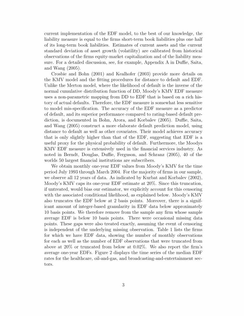
We obtain monthly one-year EDF values from Moody’s KMV for the timeperiod July 1993 through March 2004. For the majority of firms in our sample,we observe all 12 years of data. As indicated by Kurbat and Korbalev (2002),Moody’s KMV caps its one-year EDF estimate at 20%. Since this truncation,if untreated, would bias our estimator, we explicitly account for this censoringwith the associated conditional likelihood, as explained below. Moody’s KMValso truncates the EDF below at 2 basis points. Moreover, there is a signif-icant amount of integer-based granularity in EDF data below approximately10 basis points. We therefore remove from the sample any firm whose sampleaverage EDF is below 10 basis points. There were occasional missing datapoints. These gaps were also treated exactly, assuming the event of censoringis independent of the underlying missing observation. Table 1 lists the firmsfor which we have EDF data, showing the number of monthly observationsfor each as well as the number of EDF observations that were truncated fromabove at 20% or truncated from below at 0.02%. We also report the firm’saverage one-year EDFs. Figure 2 displays the time series of the median EDFrates for the healthcare, oil-and-gas, and broadcasting-and-entertainment sec-tors.
3
Tab
le1:
Des
crip
tion
ofE
DF
dat
a.Sou
rce:
Moody’s
KM
V.
ticker
secto
runcensr
d.
≥20%
≤0.0
2%
tota
lm
ean(E
DF)
ticker
secto
runcensr
d.
≥20%
≤0.0
2%
tota
lm
ean(E
DF)
253647Q
B&
E55
018
73
10
IPG
B&
E119
01
120
95
AB
CH
113
00
113
165
JN
JH
26
0118
144
2A
BT
H82
062
144
4K
MG
O&
G123
021
144
21
AD
ELQ
B&
E97
16
0113
763
KM
IO
&G
142
02
144
28
AG
NH
126
018
144
11
KM
PO
&G
139
03
142
20
AH
CO
&G
137
07
144
14
KR
IB
&E
70
050
120
4A
MG
NH
36
0108
144
4L
B&
E81
021
102
24
APA
O&
G144
00
144
30
LH
H120
00
120
215
APC
O&
G144
00
144
21
LLY
H101
043
144
5B
AX
H144
00
144
18
MC
CC
B&
E56
00
56
584
BC
B&
E120
00
120
45
MD
TH
39
0105
144
3B
EV
H142
20
144
309
MG
LH
H103
19
0122
718
BH
IO
&G
144
00
144
27
MM
MH
42
078
120
3B
JS
O&
G144
00
144
48
MR
KH
50
070
120
4B
LC
B&
E115
05
120
21
MR
OO
&G
144
00
144
29
BM
YH
54
090
144
8N
BR
O&
G144
00
144
40
BR
O&
G129
015
144
11
NEV
O&
G137
00
137
205
BSX
H123
021
144
22
NO
IO
&G
97
00
97
105
CA
HH
144
00
144
19
OC
RH
131
013
144
74
CA
MO
&G
113
00
113
55
OEI
O&
G124
00
124
94
CC
UB
&E
142
02
144
24
OM
CB
&E
120
00
120
31
CH
IRH
144
00
144
26
OX
YO
&G
132
012
144
22
CH
KO
&G
130
13
0143
520
PD
EO
&G
144
00
144
192
CH
TR
B&
E50
11
061
924
PFE
H36
084
120
2C
MC
SA
B&
E144
00
144
53
PH
AH
77
023
100
10
CN
GU
72
013
85
5PK
DO
&G
144
00
144
300
CO
CO
&G
45
00
45
25
PR
MB
&E
107
30
110
340
CO
PO
&G
133
011
144
8PX
DO
&G
144
00
144
124
CO
XB
&E
116
00
116
22
RC
LB
&E
141
00
141
80
CV
XO
&G
39
0105
144
3R
IGO
&G
136
04
140
45
CY
HH
97
00
97
124
SB
GI
B&
E113
00
113
270
DC
XC
68
06
74
41
SG
PH
61
059
120
11
DG
XH
93
00
93
103
SLB
O&
G85
035
120
15
DIS
B&
E103
041
144
10
SU
NO
&G
120
00
120
29
DO
O&
G97
010
107
27
TH
CH
144
00
144
65
DV
NO
&G
135
09
144
23
TLM
O&
G126
018
144
21
DY
NU
121
13
0134
450
TR
IH
67
00
67
180
EEP
O&
G114
06
120
15
TSG
B&
E94
03
97
47
EN
RN
QO
&G
105
11
107
44
TSO
O&
G135
00
135
168
EP
O&
G143
10
144
244
TW
X(A
OL)
B&
E144
00
144
61
EPD
O&
G76
00
76
24
UC
LO
&G
117
03
120
15
FC
143
01
144
26
UH
SH
120
00
120
30
FST
O&
G142
00
142
282
UN
HH
113
07
120
19
GD
TH
115
02
117
17
VIA
B&
E139
05
144
17
GEN
ZH
144
00
144
22
VLO
O&
G144
00
144
40
GLM
O&
G120
00
120
51
VPI
O&
G144
00
144
128
GM
C144
00
144
33
WFT
O&
G143
01
144
87
HA
LO
&G
144
00
144
52
WLP
H137
07
144
26
HC
AH
140
04
144
37
WM
BU
135
81
144
236
HC
RH
120
00
120
41
WY
EH
86
058
144
10
HM
AH
95
025
120
21
XO
MO
&G
00
120
120
2H
RC
H131
40
135
233
XT
OO
&G
120
00
120
122
HU
MH
142
00
142
86
YB
TVA
B&
E120
00
120
398
ICC
IT
65
00
65
326
tota
l11,8
94
91
1,5
45
13,5
30
*H
:H
ealt
hcare
;O
&G
:O
iland
Gas;
B&
E:B
roadcast
ing
and
Ente
rtain
ment;
C:C
ars
;T
:Tele
com
munic
ati
ons;
U:U
tiliti
es.
**
Inbasi
spoin
ts.
4

Nov00 May01 Dec01 Jul02 Jan03 Aug03 Feb0420
40
60
80
100
120
140
160
180
HealthcareBroadcasting and EntertainmentOil and GasAll
weeks
bas
ispoi
nts
Figure 1: Median one-year EDF rates by sector. Source: Moody’s KMV.
3 Parametric Model for Default Intensity
The default intensity of an obligor is the instantaneous mean arrival rate ofdefault, conditional on all current information. To be slightly more precise, wesuppose that default for a given firm occurs at the first event time of a (non-explosive) counting process N with intensity process λ, relative to a givenprobability space (Ω,F , P ) and information filtration {Ft : t ≥ 0} satisfyingthe usual conditions. In this case, so long as the obligor survives, we say thatits default intensity at time t is λt. Under mild technical conditions, this meansthat, conditional on survival to time t and all information available at time t,the probability of default between times t and t + h is approximately λth forsmall h. We also adopt the relatively standard simplifying doubly-stochastic,or Cox-process, assumption, under which the conditional probability at timet, for a currently surviving obligor, that the obligor survives to some later timeT , is
p(t, T ) = E(e−
R Tt
λ(s) ds∣∣ Ft
). (1)
We study four one-factor models for the default intensity that are a specialcase of the system of stochastic dynamic equations
dλt = [α0 + α1λt + α2λt log λt] dt + [β0 + β1λν1] dBt + γJλtΔJt. (2)
Here, α0, α1, α2, β0, and β1 are constants, ν ∈ {0.5, 1} and γJ ∈ {0, 1}.(B, Bv) is a two-dimensional standard Brownian motion and ΔJ is a pure
5

Table 2: Model specifications for actual default intensities.
Id Model α0 α1 α2 β0 β1 β2 ν γJ
OU Ornstein-Uhlenbeck√ √ √
CIR Cox-Ingersoll-Ross√ √ √
0.5
CIRJ Cox-Ingersoll-Ross w jumps√ √
0.5 1
BK Black-Karasinski√ √ √
1
jump process, whose jump sizes are independent and whose jump times arethose of an independent Poisson process with mean jump arrival rate l. Table 2gives the details for each of the six model specifications that are subject of ourstudy by showing the values of the exponent ν and the indicator γJ and byindicating with “
√” those coefficients that appear in nonzero form.
Each of the specifications in Table 2 models the default intensity as a mean-reverting stochastic and, except for the OU model, non-negative process. Thefirst three specifications OU, CIR and CIRJ belong to the class of affine pro-cesses with jump diffusions, and closed-form solutions for the survival probabil-ities in (1) are available. (See Duffie and Kan (1996) and Duffie and Garleanu(2001) for details.) The BK model is used, for example, by Berndt, Douglas,Duffie, Ferguson, and Schranz (2005) to describe the time-series behavior ofactual default arrival intensities. For this model, given the log-autoregressiveform of the default intensity in (A.5) in the appendix, there is no closed-formsolution available for the one-year EDF, 1 − p(t, t + 1) from (1). We there-fore rely on numerical lattice-based calculations of p(t, t + 1) and employ thetwo-stage Hull and White (1994) procedure for constructing trinomial trees.
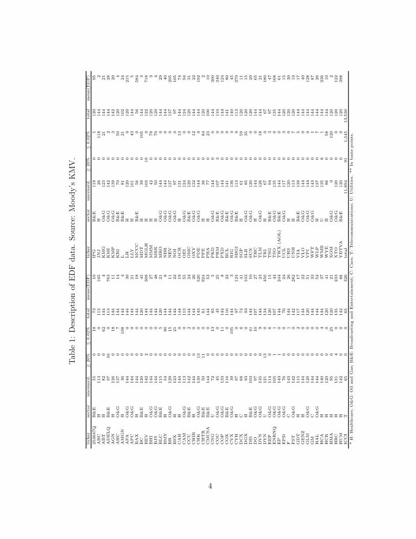
Duffee (2002) observes that excess returns on corporate bonds are (i) small,on average, and that they (ii) exhibit a substantial predictable variation. Wenow examine whether we find similar evidence for actual default intensities.Since we do not observe instantaneous default intensities directly, we will relyon the one-year EDF observations as close proxies for this exploratory analysisand compute the ratio of the sample average of one-year EDFs over the samplestandard deviation of the EDFs for each firm in our sample. Table 3 showscross-sectional summary statistics for these ratios, and Figure 2 plots a his-togram of the ratios across all firms. We find evidence that the ratio
Etλt+h
V artλt+h
can take on values both above and below one. The latter occurs, using EDFsas a proxy of λ, for roughly one-third of the firms in our sample. Compar-ing the two one-factor non-negative pure-diffusion models CIR and BK, an
6

Table 3: In-sample statistics for ratios of a firm’s average one-year EDFs totheir standard deviation
Sector mean std. dev. 1st quartile median 3rd quartile firms
Healthcare 1.221 0.480 0.885 1.151 1.389 36Oil and Gas 1.174 0.440 0.975 1.092 1.346 42B & E 1.153 0.305 0.968 1.081 1.348 21Cars 1.421 0.384 1.128 1.513 1.691 3Others 1.280 0.816 0.583 1.287 1.977 4All 1.197 0.441 0.929 1.111 1.387 106
attractive feature of the BK model is that
E(λt+h|λt)√V ar(λt+h|λt)
=eθ(1−k)λk
t e1/2s2
eθ(1−k)λkt
√e2σ2
2κ(1−k2) − e
σ2
2κ(1−k2)
=1√
eσ2
2κ(1−k2) − 1
→ 1√e
σ2
2κ − 1
as h → ∞
for all time steps h, whereas for the CIR model we have
E(λt+h|λt)√V ar(λt+h|λt)
=θ(1 − k) + kλt√
θ σ2
2κ(1 − k)2 + λt
σ2
κk(1 − k)
→√
2θκ
σas h → ∞ or as λt → 0
≥ 1 if the Feller condition is satisfied.
The BK model specification, therefore, offers the flexibility of the conditionalstandard deviation of λ to exceed the conditional mean for σ2 > 2 log(2) κ,whereas in the CIR model that is not possible in the long-run.
4 Estimation Strategy
For our analysis, we will ignore misspecification of the EDF model itself andassume that 1 − p(t, t + 1) is indeed the current one-year EDF. From theMoody’s KMV data, we then observe p(t, t + 1) at successive dates t, t + h,t + 2h, . . ., where h is one month. From these observations, we will estimate
7
0 0.5 1 1.5 2 2.5 30
2
4
6
8
10
12
14
16
18
20
mean(EDF)/std.dev.(EDF)
Figure 2: Distribution of the ratio of a firm’s average EDF over their standarddeviation.
a time-series model of the underlying intensity process λ, for each firm, underthe four different model specifications in Table 2. In total, we analyzed 106firms from seven industry groups.
The data for firm i is the one-year EDF level Y iji at month ji, for a subset
{tji0, . . . , tji
Ni} of N+1 month-end times t0, t1, . . . , tN . Our maximum likelihood
estimator (MLE) Θ of the parameter vector Θ treats the effects of missingand of truncated EDFs. For each date tj, let Oj denote the subset of firms{1, . . . , I} for which we observe an uncensored EDF rate at that time, and letCj and Mj denote the subset of firms for which the EDF data at time tj istruncated and missing, respectively. Then we can define Y O
j = {Y ij ; i ∈ Oj},
Y Cj = {Y i
j ; i ∈ Cj}, and Y Mj = {Y i
j ; i ∈ Mj} as the collection of uncensored,truncated and missing EDF observations at time tj, respectively. Finally,Yj = Y O
j ∪ Y Cj ∪ Y M
j collects all EDF data at time tj .The complete data likelihood of Y = {Yj : j = 1, . . . , N} evaluated at
outcomes y = {yj : j = 1 : N}, using the usual abuse of notation for measures,is defined by
L(Y ; Θ) dy =
N−1∏j=0
P (Yj+1 ∈ dyj+1; Yj = yj, Θ)
8
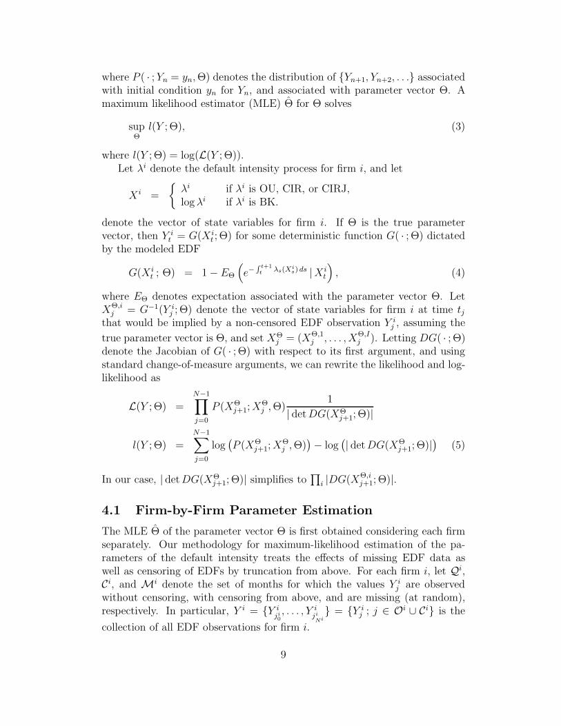
where P ( · ; Yn = yn, Θ) denotes the distribution of {Yn+1, Yn+2, . . .} associatedwith initial condition yn for Yn, and associated with parameter vector Θ. Amaximum likelihood estimator (MLE) Θ for Θ solves
supΘ
l(Y ; Θ), (3)
where l(Y ; Θ) = log(L(Y ; Θ)).Let λi denote the default intensity process for firm i, and let
X i =
{λi if λi is OU, CIR, or CIRJ,log λi if λi is BK.
denote the vector of state variables for firm i. If Θ is the true parametervector, then Y i
t = G(X it ; Θ) for some deterministic function G( · ; Θ) dictated
by the modeled EDF
G(X it ; Θ) = 1 − EΘ
(e−
R t+1t λs(Xi
s) ds |X it
), (4)
where EΘ denotes expectation associated with the parameter vector Θ. LetXΘ,i
j = G−1(Y ij ; Θ) denote the vector of state variables for firm i at time tj
that would be implied by a non-censored EDF observation Y ij , assuming the
true parameter vector is Θ, and set XΘj = (XΘ,1
j , . . . , XΘ,Ij ). Letting DG( · ; Θ)
denote the Jacobian of G( · ; Θ) with respect to its first argument, and usingstandard change-of-measure arguments, we can rewrite the likelihood and log-likelihood as
L(Y ; Θ) =
N−1∏j=0
P (XΘj+1; X
Θj , Θ)
1
| detDG(XΘj+1; Θ)|
l(Y ; Θ) =
N−1∑j=0
log(P (XΘ
j+1; XΘj , Θ)
) − log(| detDG(XΘ
j+1; Θ)|) (5)
In our case, | detDG(XΘj+1; Θ)| simplifies to
∏i |DG(XΘ,i
j+1; Θ)|.
4.1 Firm-by-Firm Parameter Estimation
The MLE Θ of the parameter vector Θ is first obtained considering each firmseparately. Our methodology for maximum-likelihood estimation of the pa-rameters of the default intensity treats the effects of missing EDF data aswell as censoring of EDFs by truncation from above. For each firm i, let Qi,Ci, and Mi denote the set of months for which the values Y i
j are observedwithout censoring, with censoring from above, and are missing (at random),respectively. In particular, Y i = {Y i
ji0, . . . , Y i
jiNi} = {Y i
j ; j ∈ Oi ∪ Ci} is the
collection of all EDF observations for firm i.
9

Suppose, to pick an example of a censoring outcome from which the generalcase can easily be deduced, that, for months k through k > k+1 inclusive, theEDFs are truncated at ζ = 20%. That means that the censored and observedvalue Y i
j is 20%, implying that the actual EDF was equal to or larger than20%. Let us also assume that the EDF data between months l + 1 and l,inclusive, are missing, but that we have EDF observations without censoringfor all other months. That is, Oi = {0, . . . , k, k + 1, . . . , l, l + 1, . . . , N}, Ci ={j : k + 1 ≤ j ≤ k}, and Mi = {j : l + 1 ≤ j ≤ l}. Then, the likelihood ofthe EDF observations Y i evaluated at outcomes y = {yj : j ∈ Oi}, using theusual abuse of notation for measures, is defined by
L(Y i ; Θ) dy =
k−1∏j=0
P (Y ij+1 ∈ dyj+1; Y
ij = yj, Θ)
×P (Y ik+1 ≥ ζ, . . . , Y i
k ≥ ζ ; Y ik = yk, Y
ik+1 = yk+1, Θ)
×P (Y ik+1 ∈ dyk+1 ; Y i
k = yk, Θ)
×l−1∏
j=k+1
P (Y ij+1 ∈ dyj+1; Y
ij = yj, Θ)
×P (Y il+1 ∈ dyl+1; Y
il = yl, Θ)
×N−1∏
j=l+1
P (Y ij+1 ∈ dyj+1; Y
ij = yj, Θ),
Using standard change-of-measure arguments, we can rewrite the likelihood as
L(Y i ; Θ) dy =
k−1∏j=0
P (XΘ,ij+1 ; XΘ,i
j , Θ)1
| detDG(XΘ,ij+1 ; Θ)|
×P (Y ik+1 ≥ ζ, . . . , Y i
k ≥ ζ ; Y ik = yk, Y
ik+1 = yk+1, Θ)
×P (XΘ,i
k+1; XΘ,i
k , Θ)1
| detDG(XΘ,i
k+1; Θ)|
×l−1∏
j=k+1
P (XΘ,ij+1 ; XΘ,i
j , Θ)1
| detDG(XΘ,ij+1; Θ)|
×P (XΘ,i
l+1; XΘ,i
l , Θ)1
| detDG(XΘ,i
l+1; Θ)|
×N−1∏
j=l+1
P (XΘ,ij+1 ; XΘ,i
j , Θ)1
| detDG(XΘ,ij+1; Θ)| . (6)
10

The second term on the right-hand side of (6) is equal to
q(Y i ; Θ) = P (XΘ,ik+1 ≥ G−1(ζ ; Θ), . . . , XΘ,i
k≥ G−1(ζ ; Θ) ;
XΘ,ik = G−1(yk; Θ), XΘ,i
k+1= G−1(yk+1; Θ), Θ).
In Appendix A we describe, for each of the model specifications in Table 2,how to compute q(Y ; Θ) by Monte Carlo integration.
A MLE Θi for Θ of firm i solves
supΘ
L(Y i ; Θ). (7)
The firm-by-firm parameter estimates are summarized in Table 4.
4.2 Sector-by-Sector Parameter Estimation
A Monte-Carlo analysis revealed substantial small-sample bias in the MLEestimators, especially for mean reversion. We therefore impose that all firmswithin one industry have the same level of mean reversion κ and volatility σ,while allowing for a firm-specific level parameter θ. The Brownian motionsdriving the default intensities have a constant pairwise correlation across allfirms in the sector. For example, for the BK model, we generalize (2) byassuming that X i
t of firm i satisfies the Ornstein-Uhlenbeck equation
dX it = κ
(θi − X i
t
)dt + σ
(√ρ dBc
t +√
1 − ρ dBit
), (8)
where Bc and Bi are independent standard Brownian motions, independentof {Bj}j �=i, and the constant pairwise within-sector correlation coefficient ρ isan additional parameter to be estimated.
We then employ the Expectation-Maximization (EM) algorithm to find amaximum likelihood estimator Θ. The EM algorithm starts with an initialguess Θ(0) and iterates the following two steps:
• E-step: Compute
Q(Θ|Θ(m)) = E[l(Y ; Θ)|Yo, Θ(m)] (9)
• M-step: Find Θ(m+1) that maximizes l(Θ|Θ(m)).
It is well known that this iteration always increases the likelihood value (see,for example, Dempster, Lair, and Rubin (1977)). We stop the iteration if thechange in the parameters falls below ε, for ε small.
11

Table 4: Summary statistics for fitted parameters.
Parameter OU CIR CIRJ BKα0
mean 23.23 18.32 18.83std dev 55.91 44.23 47.15median 1.99 6.08 6.161st quartile 0.65 4.01 4.183rd quartile 15.17 14.01 14.45α1 α1 − 1
2β21
mean 0.50 0.09 0.17 1.59std dev 0.43 0.17 0.29 1.47median 0.48 0.03 0.01 0.981st quartile 0.07 0.00 0.00 0.633rd quartile 0.75 0.12 0.22 1.89α2
mean 0.53std dev 0.41median 0.381st quartile 0.273rd quartile 1.53β0
mean 253.14std dev 369.74median 66.791st quartile 27.313rd quartile 354.00β1
mean 4.86 4.64 1.35std dev 3.63 3.62 0.40median 3.48 3.46 1.311st quartile 2.83 2.86 1.123rd quartile 5.28 4.74 1.53γJ
mean 4.22std dev 35.75median 0.031st quartile 0.013rd quartile 0.08
12

In our analysis we will approximate the expectation in (9) by its MC esti-mate. Using a standard change of variable argument, the expectation in (9)can be written as∫
l(Y (X); Θ)fX(XC, XM|XO, Θ(m)) d(xC, xM).
We use the Systematic-Scan Gibbs Sampler (see, for example, Liu (2003))to impute censored and missing data points. Initially, we set all componentsof Y C equal to 20% and initialize all missing data points in Y M via linearinterpolation. Define Y CM = (Y C, Y M) and align Ycm = (Ycm,1, . . . , Ycm,N),and similarly for the associated X. At the (g + 1)-st iteration of the GibbsSampler:
• Draw, for j = 2, . . . , N , XCM,(g+1)j from the conditional distribution
fX(XCM,(g+1)j |XCM,(g+1)
1 , . . . , XCM,(g+1)j−1 , X
CM,(g+1)j+1 , . . . , X
CM,(g+1)N ; XO; Θ)
The proof of the following lemma is provided in Appendix B.
Lemma 1. Let S = {1, . . . , S} denote some subset of firms {1, . . . , I} and letSc be its complement. Let’s fix some time point tj between t0 and tN . Then,the conditional distribution of XSc,j given Xj−1, XS,j, and Xj+1 is normal withmean μ = wμ1 + (1− w)μ2 and variance-covariance matrix Σ = wA−1
22 , wherew = (1 + e−2κh)−1, A21 and A22 are the lower-left (I − S)× S and lower-right(I − S) × (I − S) submatrix of Σ−1
ε , respectively, and
μ1 = θSc + e−κh(XSc,j−1 − θSc) − (A22)−1A21εS,j,
μ2 = θSc + eκh(XSc,j+1 − θSc) + eκh(A22)−1A21εS,j+1.
Sector-by-sector estimates for the BK model are shown in Table 5, withasymptotic standard error estimates in parentheses. Note that the ML esti-mates for the correlation parameter ρ are quite different for different industrygroups. It is higher among oil and gas companies, and lower for healthcarefirms. This is confirmed when computing the average pairwise correlation ofthe firms’ innovations to log EDFs by sector, which are reported in Table 6.
Note that according to Figure 2 the healthcare sector has, at least on aver-age, the firms with the highest credit-quality, whereas oil and gas companiesare more often of medium credit quality. Table 7 shows the average pairwisecorrelation of innovations to log EDFs for firms in different median-EDF brack-ets. For our sample period, pairwise correlation seem to be lower among firmswith very low default risk and also among firms with a very high probabilityof default. They are higher among firms of median credit quality. As shown inAppendix C, however, the pairwise correlation between λi and λj in the BKmodel does not depend on θi, θj or the level of λ.
13
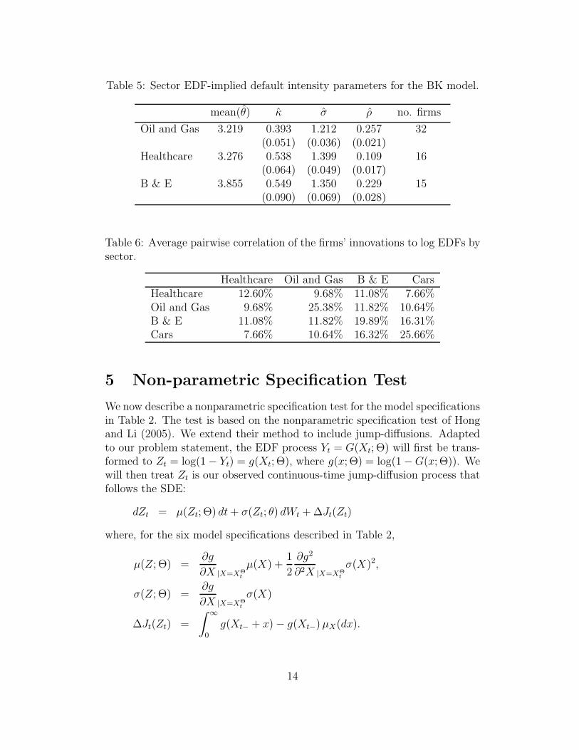
Table 5: Sector EDF-implied default intensity parameters for the BK model.
mean(θ) κ σ ρ no. firms
Oil and Gas 3.219 0.393 1.212 0.257 32(0.051) (0.036) (0.021)
Healthcare 3.276 0.538 1.399 0.109 16(0.064) (0.049) (0.017)
B & E 3.855 0.549 1.350 0.229 15(0.090) (0.069) (0.028)
Table 6: Average pairwise correlation of the firms’ innovations to log EDFs bysector.
Healthcare Oil and Gas B & E CarsHealthcare 12.60% 9.68% 11.08% 7.66%Oil and Gas 9.68% 25.38% 11.82% 10.64%B & E 11.08% 11.82% 19.89% 16.31%Cars 7.66% 10.64% 16.32% 25.66%
5 Non-parametric Specification Test
We now describe a nonparametric specification test for the model specificationsin Table 2. The test is based on the nonparametric specification test of Hongand Li (2005). We extend their method to include jump-diffusions. Adaptedto our problem statement, the EDF process Yt = G(Xt; Θ) will first be trans-formed to Zt = log(1 − Yt) = g(Xt; Θ), where g(x; Θ) = log(1 − G(x; Θ)). Wewill then treat Zt is our observed continuous-time jump-diffusion process thatfollows the SDE:
dZt = μ(Zt; Θ) dt + σ(Zt; θ) dWt + ΔJt(Zt)
where, for the six model specifications described in Table 2,
μ(Z; Θ) =∂g
∂X |X=XΘt
μ(X) +1
2
∂g2
∂2X |X=XΘt
σ(X)2,
σ(Z; Θ) =∂g
∂X |X=XΘt
σ(X)
ΔJt(Zt) =
∫ ∞
0
g(Xt− + x) − g(Xt−) μX(dx).
14
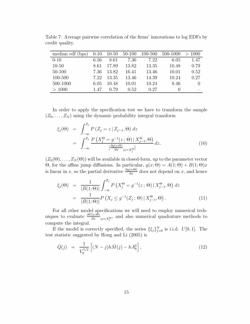
Table 7: Average pairwise correlation of the firms’ innovations to log EDFs bycredit quality.
median edf (bps) 0-10 10-50 50-100 100-500 500-1000 > 10000-10 6.56 8.61 7.36 7.22 6.05 1.4710-50 8.61 17.89 13.82 13.35 10.48 0.7950-100 7.36 13.82 16.41 13.46 10.01 0.52100-500 7.22 13.35 13.46 14.39 10.24 0.27500-1000 6.05 10.48 10.01 10.24 8.46 0> 1000 1.47 0.79 0.52 0.27 0 –
In order to apply the specification test we have to transform the sample(Z0, . . . , ZN) using the dynamic probability integral transform
ξj(Θ) =
∫ Zj
−∞P (Zj = z |Zj−1, Θ) dz
=
∫ Zj
−∞
P(XΘ
j = g−1(z ; Θ) |XΘj−1, Θ
)|∂g(x;Θ)
∂x |x=XΘj|
dz. (10)
(Z0(Θ), . . . , ZN(Θ)) will be available in closed-form, up to the parameter vectorΘ, for the affine jump diffusions. In particular, g(x; Θ) = A(1; Θ) + B(1; Θ)x
is linear in x, so the partial derivative ∂g(x;Θ)∂x
does not depend on x, and hence
ξj(Θ) =1
|B(1; Θ)|∫ Zj
−∞P
(XΘ
j = g−1(z ; Θ) |XΘj−1, Θ
)dz
=1
|B(1; Θ)|P(Xj ≤ g−1(Zj ; Θ) |XΘ
j−1, Θ). (11)
For all other model specifications we will need to employ numerical tech-niques to evaluate ∂G(x;Θ)
∂x |x=XΘt, and also numerical quadrature methods to
compute the integral.If the model is correctly specified, the series {ξj}N
j=0 is i.i.d. U [0, 1]. Thetest statistic suggested by Hong and Li (2005) is
Q(j) =1
V1/20
[(N − j)hM(j) − hA0
h
], (12)
15

where h = h(n) is a bandwidth such that h → 0 and nh → ∞ as n → ∞, and
M(j) =
∫ 1
0
∫ 1
0
(ηj(z1, z2) − 1)2 dz1 dz2
ηj(z1, z2) =1
N − j
N∑τ=j+1
Kh(z1, ξτ)Kh(z2, ξτ−j)
Kh(x, y) =
⎧⎪⎪⎪⎨⎪⎪⎪⎩
1h
k(x−yh )
R 1−x/h
k(u) duif x ∈ [0, h)
1hk
(x−y
h
)if x ∈ [h, 1 − h]
1h
k(x−yh )
R (1−x)/h−1 k(u) du
if x ∈ (1 − h, 1]
k(u) =15
16(1 − u2)21{|u|≤1}.
The non-stochastic centering and scaling factors are
A0h =
[(1
h− 2)
∫ 1
−1
k2(u) du + 2
∫ 1
0
∫ b
−1
k2b (u)k2(u) du db
]2
− 1,
V0 = 2
[∫ 1
−1
(∫ 1
−1
k(u + v)k(v) dv
)2
du
]2
,
kb(·) =k(·)∫ b
−1k(v) dv
.
As suggested in Hong and Li (2005), we use h = n−1/6std({ξ}). Under thecorrect model specification, Hong and Li (2005) show that
Q(j) →d N(0, 1), (13)
cov(Q(i), Q(j)) →p 0 for i = j (14)
Under model misspecification, on the other hand, we have
Q(j) →p ∞.
Hence, we compare the test statistic Q(j) with the upper-tailed N(0, 1) criticalvalue Cα at the level α and, if Q(j) > Cα, reject the null hypothesis of correctmodel specification at level α.
Figure 3 plots the histogram of generalized residuals, across all firms, andFigure 4 displays the Q(j) test statistics, j = 1, . . . , 20, for the OU, CIR andBK model specifications. Finally, Table 8 shows the rejection rates based onQ(1) statistics for 106 firms in our sample.
16

0 0.25 0.5 0.75 10
200
400
600
800
1000
1200
CIR
0 0.25 0.5 0.75 10
200
400
600
800
1000
1200
OU
0 0.25 0.5 0.75 10
200
400
600
800
1000
1200
BK
Figure 3: Histogram of generalized residuals, across all firms.
0 5 10 15 200
5
10
15
20
25
30
35
40
45
Lag
Q S
tatis
tics
(me
dia
n)
OUCIRBK
Figure 4: Q(j) test for default intensity model specifications.
17

Table 8: Rejection rates based on Q(1) statistics.
Significance OU CIR BKLevel
1% 0.988 0.724 0.408
5% 0.988 0.803 0.539
10% 1.000 0.855 0.553
18

A Discussion of Model Specifications
In this appendix, we study the model specifications in Table 2 of actual defaultintensities with regard to (i) their functional form of G(X i
t ; Θ) in (4), (ii) thetransition densities P ( · ; X i
j , Θ), and (iii) simulating missing and censoreddata from P ( · ; X i
k, Xik+1
, Θ).
A.1 OU Model
In the Ornstein-Uhlenbeck model specification, the state variable X equals λand follows the stochastic process
dXt = κ(θ − Xt) dt + σ dBt, (A.1)
For (A.1), G is available in closed form
G(x ; Θ) = 1 − eA(1 ;Θ)+B(1 ; Θ)x,
where k = e−κΔ and
A(Δ ; Θ) = −θ
(Δ +
1 − k
κ
)+
1
2
σ2
κ2
(Δ + 2
1 − k
κ− 1 − k2
2κ
),
B(Δ ; Θ) = −1 − k
κ.
The conditional transition probability P (Xt+Δ ; Xt, Θ) is normal with condi-tional mean (1 − k)θ + kXt and conditional variance σ2
2κ(1 − k2).
We observe that for any time t between times s and u, the conditional dis-tribution of Xt given Xs and Xu is a normal distribution with mean M(t | s, u)and variance V (t | s, u) given by
M(t | s, u) =1 − e−2κ(u−t)
1 − e−2κ(u−s)M(t | s) +
e−2κ(u−t) − e−2κ(u−s)
1 − e−2κ(u−s)M(t | u),
V (t | s, u) =V (t | s)V (u | t)
V (u | s) ,
where, for times t before u, we let
M(u | t) = θ + e−κ(u−t)(X(t) − θ)
V (u | t) =σ2
2κ(1 − e−2κ(u−t))
M(t | u) = eκ(u−t)(X(u) − θ(1 − e−κ(u−t)))
denote the conditional expectation and variance, respectively, of Xu given Xt,and the conditional expectation of Xt given Xu. As a consequence, letting
19

Zk = X(tk), we can easily simulate from the joint conditional distribution of(Zk+1, . . . , Zk) given Zk and Zk+1 which is given by
P (Zk+1, . . . , Zk |Zk, Zk+1) = P (Zk+1 |Zk, Zk+1)
k−(k+1)∏j=1
P (Zk+j+1 |Zk+j, Zk+1).
We are now in a position to estimate the quantity in (7) by generating some“large” integer number J of independent sample paths {(Zj
k+1, . . . , Zj
k); 1 ≤
j ≤ J} from the joint conditional distribution of (Zk+1, . . . , Zk) given Zk andZk+1, and by computing the fraction of those paths for which Zj
i ≥ g−1(ζ) forall i in {k + 1, . . . , k}.
A.2 CIR Model
In the Cox-Ingersoll-Ross model specification, the state variable X equals λand follows the stochastic process
dXt = κ(θ − Xt) dt + σ√
Xt dBt, (A.2)
For (A.1), G is available in closed form
G(x ; Θ) = 1 − eA(1 ;Θ)+B(1 ; Θ)x,
where (see, for example, Duffie and Garleanu (2001))
B(Δ ; Θ) =1 − eb1s
c1 + d1eb1Δ
A(Δ ; Θ) =m(−c1 − d1)
b1c1d1log
c1 + d1eb1s
c1 + d1+
m
c1s,
where, with n = −κ, p = σ2, and m = κθ, we have
c1 =−n +
√n2 − 2pq
2q
d1 =n +
√n2 − 2pq
2q
b1 = −d1(n + 2qc1) − (nc1 + p)
c1 − d1.
A.3 CIRJ Model
The default intensity follows an (CIRJ) process with jumps:
dXt = κ(θ − Xt) dt + σ√
Xt dBt + ΔJt, (A.3)
20
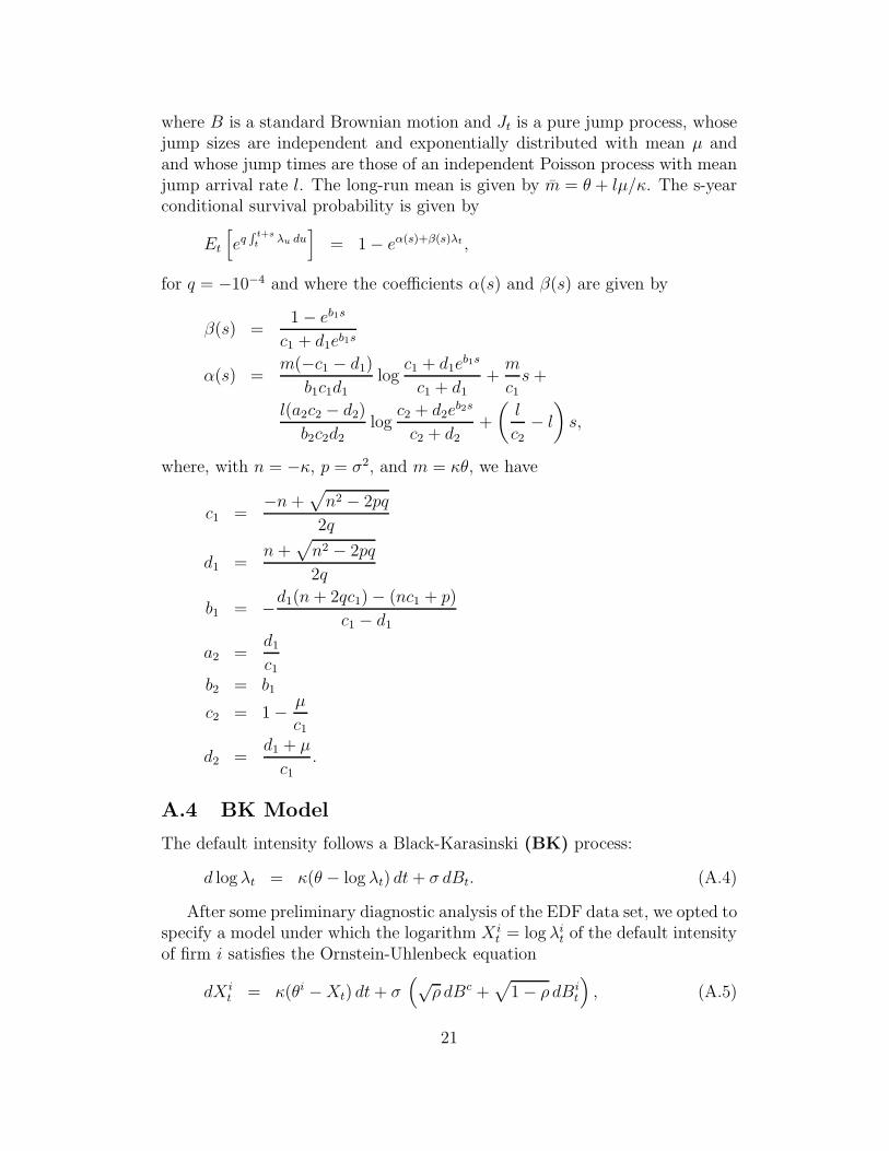
where B is a standard Brownian motion and Jt is a pure jump process, whosejump sizes are independent and exponentially distributed with mean μ andand whose jump times are those of an independent Poisson process with meanjump arrival rate l. The long-run mean is given by m = θ + lμ/κ. The s-yearconditional survival probability is given by
Et
[eq
R t+st
λu du]
= 1 − eα(s)+β(s)λt ,
for q = −10−4 and where the coefficients α(s) and β(s) are given by
β(s) =1 − eb1s
c1 + d1eb1s
α(s) =m(−c1 − d1)
b1c1d1log
c1 + d1eb1s
c1 + d1+
m
c1s +
l(a2c2 − d2)
b2c2d2log
c2 + d2eb2s
c2 + d2+
(l
c2− l
)s,
where, with n = −κ, p = σ2, and m = κθ, we have
c1 =−n +
√n2 − 2pq
2q
d1 =n +
√n2 − 2pq
2q
b1 = −d1(n + 2qc1) − (nc1 + p)
c1 − d1
a2 =d1
c1
b2 = b1
c2 = 1 − μ
c1
d2 =d1 + μ
c1
.
A.4 BK Model
The default intensity follows a Black-Karasinski (BK) process:
d log λt = κ(θ − log λt) dt + σ dBt. (A.4)
After some preliminary diagnostic analysis of the EDF data set, we opted tospecify a model under which the logarithm X i
t = log λit of the default intensity
of firm i satisfies the Ornstein-Uhlenbeck equation
dX it = κ(θi − Xt) dt + σ
(√ρ dBc +
√1 − ρ dBi
t
), (A.5)
21
where B =(Bc, B1, . . . , BI
)′is a I + 1-dimensional standard Brownian mo-
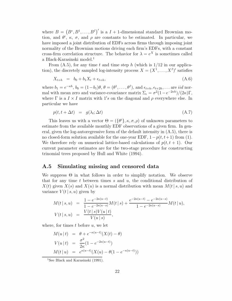
tion, and θi, κ, σ, and ρ are constants to be estimated. In particular, wehave imposed a joint distribution of EDFs across firms through imposing jointnormality of the Brownian motions driving each firm’s EDFs, with a constantcross-firm correlation structure. The behavior for λ = eX is sometimes calleda Black-Karasinski model.1
From (A.5), for any time t and time step h (which is 1/12 in our applica-tion), the discretely sampled log-intensity process X = (X1, . . . , XI)′ satisfies
Xt+h = b0 + b1Xt + εt+h, (A.6)
where b1 = e−κh, b0 = (1−b1)θ, θ = (θ1, . . . , θI), and εt+h, εt+2h, . . . are iid nor-mal with mean zero and variance-covariance matrix Σε = σ2(1−e−2κh)/(2κ)Γ,where Γ is a I × I matrix with 1′s on the diagonal and ρ everywhere else. Inparticular we have
p(t, t + Δt) = g(λt; Δt) (A.7)
This leaves us with a vector Θ = ({θi}, κ, σ, ρ) of unknown parameters toestimate from the available monthly EDF observations of a given firm. In gen-eral, given the log-autoregressive form of the default intensity in (A.5), there isno closed-form solution available for the one-year EDF, 1−p(t, t+1) from (1).We therefore rely on numerical lattice-based calculations of p(t, t + 1). Ourcurrent parameter estimates are for the two-stage procedure for constructingtrinomial trees proposed by Hull and White (1994).
A.5 Simulating missing and censored data
We suppress Θ in what follows in order to simplify notation. We observethat for any time t between times s and u, the conditional distribution ofX(t) given X(s) and X(u) is a normal distribution with mean M(t | s, u) andvariance V (t | s, u) given by
M(t | s, u) =1 − e−2κ(u−t)
1 − e−2κ(u−s)M(t | s) +
e−2κ(u−t) − e−2κ(u−s)
1 − e−2κ(u−s)M(t | u),
V (t | s, u) =V (t | s)V (u | t)
V (u | s) ,
where, for times t before u, we let
M(u | t) = θ + e−κ(u−t)(X(t) − θ)
V (u | t) =σ2
2κ(1 − e−2κ(u−t))
M(t | u) = eκ(u−t)(X(u) − θ(1 − e−κ(u−t)))
1See Black and Karasinski (1991).
22
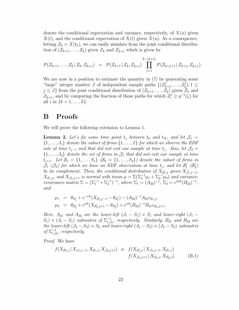
denote the conditional expectation and variance, respectively, of X(u) givenX(t), and the conditional expectation of X(t) given X(u). As a consequence,letting Zk = X(tk), we can easily simulate from the joint conditional distribu-tion of (Zk+1, . . . , Zk) given Zk and Zk+1 which is given by
P (Zk+1, . . . , Zk |Zk, Zk+1) = P (Zk+1 |Zk, Zk+1)
k−(k+1)∏j=1
P (Zk+j+1 |Zk+j, Zk+1).
We are now in a position to estimate the quantity in (7) by generating some“large” integer number J of independent sample paths {(Zj
k+1, . . . , Zj
k); 1 ≤
j ≤ J} from the joint conditional distribution of (Zk+1, . . . , Zk) given Zk andZk+1, and by computing the fraction of those paths for which Zj
i ≥ g−1(ζ) forall i in {k + 1, . . . , k}.
B Proofs
We will prove the following extension to Lemma 1.
Lemma 2. Let’s fix some time point tj between t0 and tN , and let J1 ={1, . . . , J1} denote the subset of firms {1, . . . , I} for which we observe the EDFrate at time tj−1 and that did not exit our sample at time tj. Also, let J2 ={1, . . . , J2} denote the set of firms in J1 that did not exit our sample at timetj+1. Let S1 = {1, . . . , S1} (S2 = {1, . . . , S2}) denote the subset of firms inJ1 (J2) for which we have an EDF observation at time tj, and let Sc
1 (Sc2)
be its complement. Then, the conditional distribution of XSc1 ,j given XJ1,j−1,
XS1,j, and XJ2,j+1 is normal with mean μ = Σ(Σ−11 μ1 + Σ−1
2 μ2) and variance-covariance matrix Σ = (Σ−1
1 +Σ−12 )−1, where Σ1 = (A22)
−1, Σ2 = e2κh(B22)−1,
and
μ1 = θSc1+ e−κh(XSc
1,j−1 − θSc1) − (A22)
−1A21εS1,j,
μ2 = θSc2+ eκh(XSc
2,j+1 − θSc2) + eκh(B22)
−1B21εS2,j+1.
Here, A21 and A22 are the lower-left (J1 − S1) × S1 and lower-right (J1 −S1) × (J1 − S1) submatrix of Σ−1
ε,J1, respectively. Similarly, B21 and B22 are
the lower-left (J2 − S2) × S2 and lower-right (J2 − S2) × (J2 − S2) submatrixof Σ−1
ε,J2, respectively.
Proof. We have
f(XSc1,j |XJ1,j−1, XS1,j, XJ2,j+1) α f(XSc
1,j |XJ1,j−1, XS1,j)
f(XJ2,j+1 |XS2,j, XSc2 ,j). (B.1)
23

For the first term on the right-hand side of (B.1) we have
XSc1,j |XJ1,j−1, XS1,j ∼ θSc
1+ e−κh(XSc
1,j−1 − θSc1) + εSc
1 ,j | εS1,j
∼ MN (μ1, Σ1) . (B.2)
Working towards the second term on the right-hand side of (B.1) we know
XJ2,j+1 |XS2,j, XSc2,j ∼ θJ2 + e−κh(XJ2,j − θJ2) + εJ2,j+1
∼ θJ2 + e−κh(XJ2,j − θJ2) + MN (0, Σε,J2) .
Hence,
log(f(XJ2,j+1 |XS2,j, XSc
2,j))
α −1
2(ε′S2,j+1, ε
′Sc
2,j+1)Σ−1ε,J2
(ε′S2,j+1, ε′Sc
2,j+1)′
In particular, the right-hand side of this equation is
−1
2(ε′S2,j+1, (XSc
2,j+1 − (θSc2+ e−κh(XSc
2,j − θSc2)))′)Σ−1
ε,J2
(ε′S2,j+1, (XSc2,j+1 − (θSc
2+ e−κh(XSc
2,j − θSc2)))′)′,
which equals, up to a constant,
− 1
2
(e−2κhX ′
Sc2,jB22XSc
2 ,j − 2e−κhX ′Sc
2 ,jB21εS2,j+1
)− 1
2
(−2e−κhX ′
Sc2,jB22(XSc
2 ,j+1 − θSc2(1 − e−κh))
)Consequently,
f(XJ2,j+1 |XS2,j, XSc2,j)
α MNpdf(XSc
2 ,j; θSc2+ eκh(XSc
2,j+1 − θSc2) + eκhB−1
22 B21εS2,j+1, e2κhB−1
22
)= MNpdf
(XSc
2 ,j; μ2, Σ2
)(B.3)
From Equations (B.2) and (B.3), we conclude that
XSc1,j |XJ1,j−1, XS1,j, XJ2,j+1 ∼ MN(μ, Σ).
24

C Implied Correlation Structure for BK Model
For the BK model in (8) we have
ρi,j = CORRt(λit+h, λ
jt+h)
=COVt(λ
it+h, λ
jt+h)√
V art(λit+h)
√V art(λ
jt+h)
=COVt(λ
it+h, λ
jt+h)√
V art(λit+h)
√V art(λ
jt+h)
=Et
[(λi
t+h − emit(h)+1/2vi
t(h))(λjt+h − emj
t (h)+1/2vjt (h))
]√
e2mit(h)+vi
t(h)(evit(h) − 1)
√e2mj
t (h)+vjt (h)(evj
t (h) − 1)
=Et
[λi
t+hλjt+h
]+ emi
t(h)+1/2vit(h)emj
t (h)+1/2vjt (h)√
e2mit(h)+vi
t(h)(evit(h) − 1)
√e2mj
t (h)+vjt (h)(evj
t (h) − 1)
=e−1/2(vi
t(h)+vjt (h))Et
[eui
t+heujt+h
]− 1√
evit(h) − 1
√evj
t (h) − 1
=e−1/2(vi
t(h)+vjt (h))e1/2V ar(ui
t+h+ujt+h) − 1√
evit(h) − 1
√evj
t (h) − 1
=e−1/2(vi
t(h)+vjt (h))e1/2V ar(ui
t+h+ujt+h) − 1√
evit(h) − 1
√evj
t (h) − 1
=e−1/2(vi
t(h)+vjt (h))e1/2(vi
t(h)+vjt (h)+2ρi,j
u
√vi
t(h)√
vjt (h)) − 1√
evit(h) − 1
√evj
t (h) − 1
=eρi,j
u
√vi
t(h)√
vjt (h) − 1√
evit(h) − 1
√evj
t (h) − 1,
where
mit(h) = θi + e−κih(log(λi
t) − θi)
vit(h) = σi21 − e−2κih
2κ.
In particular, the pairwise correlation between λi and λj does not depend onθi, θj or the level of λi
t or λjt .
25
References
Berndt, A., R. Douglas, D. Duffie, M. Ferguson, and D. Schranz (2005).
Measuring Default Risk Premia from Default Swap Rates and EDFs.
Working Paper, Stanford University.
Black, F. and P. Karasinski (1991). Bond and Option Pricing when Short
Rates are Log-Normal. Financial Analysts Journal , 52–59.
Black, F. and M. Scholes (1973). The Pricing of Options and Corporate
Liabilities. Journal of Political Economy 81, 637-654.
Bohn, J., N. Arora, and I. Korbalev (2005). Power and Level Validation of
the EDF CRedit Measure in the U.S. Market. Working Paper, Moody’s
KMV.
Crosbie, P. and J. Bohn (2001). Modeling Default Risk. Working Paper,
KMV.
Dempster, A. P., N. M. Lair, and D. B. Rubin (1977). Maximum Likelihood
from Incomplete Data via EM Algorithm. Journal of the Royal Statistical
Society, Series B 39, 1-38.
Duffee, G. R. (2002). Term Premia and Interest Rate Forecasts in Affine
Models. Journal of Finance 57, 405-43.
Duffie, D. and N. Garleanu (2001). Risk and Valuation of Collateralized
Debt Obligations. Financial Analysts Journal 57, January–February,
41–62.
Duffie, D., L. Saita, and K. Wang (2005). Multiperiod Corporate Default
Probabilities with Stochastic Covariates. forthcoming, Journal of Finan-
cial Economics.
Duffie, D. J. and R. Kan (1996). A Yield-Factor Model of Interest Rates.
Mathematical Finance 6, 379-406.
Hong, Y. and H. Li (2005). Nonparametric Specification Testing for
Continuous-Time Models with Applications to Term Structure of In-
terest Rates. RFS 18, 37-84.
Hull, J. and A. White (1994). Numerical Procedures for Implementing Term
Structure Models I: Single Factor Models. Journal of Derivatives 2, 7-
16.
26

Kealhofer, S. (2003). Quantifying Credit Risk I: Default Prediction. Finan-
cial Analysts Journal , January–February, 30–44.
Kurbat, M. and I. Korbalev (2002). Methodology for Testing the Level
of the EDF Credit Measure. Working Paper, Technical Report 020729,
Moody’s KMV.
Liu, J. S. (2003). Monte Carlo Strategies in Scientific Computing. New York,
NY: Springer Series in Statistics.
Merton, R. C. (1974). On the Pricing of Corporate Debt: The Risk Structure
of Interest Rates. Journal of Finance 29, 449-70.
27