This article was downloaded by: [Universitat Politècnica de València]On: 26 October 2014, At: 06:26Publisher: Taylor & FrancisInforma Ltd Registered in England and Wales Registered Number: 1072954 Registered office: Mortimer House,37-41 Mortimer Street, London W1T 3JH, UK

Journal of the American Statistical AssociationPublication details, including instructions for authors and subscription information:http://www.tandfonline.com/loi/uasa20

Spatial Smoothing of Geographically Aggregated Data,with Application to the Construction of Incidence MapsHans-Georg Müller a , Ulrich Stadtmüller b & Farzaneh Tabnak ca Division of Statistics , University of California , Davis , CA , 95616 , USAb Department of Mathematics , Universität Ulm , Ulm , 89069 , Germanyc California Department of Health Services , Office of AIDS, HIV-Epidemiology Branch ,Sacramento , CA , 94234 , USAPublished online: 17 Feb 2012.

To cite this article: Hans-Georg Müller , Ulrich Stadtmüller & Farzaneh Tabnak (1997) Spatial Smoothing of GeographicallyAggregated Data, with Application to the Construction of Incidence Maps, Journal of the American Statistical Association,92:437, 61-71, DOI: 10.1080/01621459.1997.10473603

To link to this article: http://dx.doi.org/10.1080/01621459.1997.10473603

PLEASE SCROLL DOWN FOR ARTICLE

Taylor & Francis makes every effort to ensure the accuracy of all the information (the “Content”) containedin the publications on our platform. However, Taylor & Francis, our agents, and our licensors make norepresentations or warranties whatsoever as to the accuracy, completeness, or suitability for any purpose of theContent. Any opinions and views expressed in this publication are the opinions and views of the authors, andare not the views of or endorsed by Taylor & Francis. The accuracy of the Content should not be relied upon andshould be independently verified with primary sources of information. Taylor and Francis shall not be liable forany losses, actions, claims, proceedings, demands, costs, expenses, damages, and other liabilities whatsoeveror howsoever caused arising directly or indirectly in connection with, in relation to or arising out of the use ofthe Content.

This article may be used for research, teaching, and private study purposes. Any substantial or systematicreproduction, redistribution, reselling, loan, sub-licensing, systematic supply, or distribution in anyform to anyone is expressly forbidden. Terms & Conditions of access and use can be found at http://www.tandfonline.com/page/terms-and-conditions

Spatial Smoothing of Geographically Aggregated Data, With Application to the Construction of

Incidence Maps Hans-Georg MULLER, Ulrich STADTMULLER, and Farzaneh TABNAK

We address the commonly encountered situation in spatial statistics where data such as counts of incidences of a certain disease are available only in geographically aggregated form. We develop fairly general models and propose a modified version of the locally weighted least squares method to recover the unknown smooth spatial function that is assumed to generate the observations. In the special case of count data, the target function is the intensity function, conditional on the total number of observations. Our method avoids the arbitrariness of selecting a point within each geographic area at which the measurement for the whole area is supposed to be located. We derive basic asymptotic properties, and apply our methods to acquired immune deficiency syndrome (AIDS) incidence data in San Francisco for 1980-1992, where counts are available aggregated over zip code areas. KEY WORDS: Aggregated count data; Aggregated regression data; Contour map; Locally weighted least squares; Monte Carlo

integration; Spatiotemporal estimation.

1. INTRODUCTION AND STATISTICAL MODEL

In various spatial datasets, available data do not carry ex- act geographical coordinates pinpointing the exact location on the map where they have been obtained. Instead, the observations falling within the same administrative bound- aries are lumped together and only an aggregated quantity, observed within a defined geographical entity like a zip code area, county, province, or state, is available. Exam- ples of such situations are abundant in the literature (see, e.g., Cressie 1992). In particular, spatial incidence data of interest in epidemiology and environmental sciences often are of this form.

Commonly available methods for smoothing such data do not take into account the aggregated nature of the data and require selection of one point within each geographical area over which data are aggregated, referred hitherto as the aggregation area. The aggregated measurement is then as- cribed to this point, and classical nonparametric smoothing procedures or kriging methods are applied. (For illustra- tive comparisons between classical nonparametric regres- sion and kriging, see Laslett 1994 and Szidarovsky and Yakowitz 1985; for an example of an epidemiological appli- cation of kriging, see Carrat and Valleron 1992.) The prob- lem of spatial aggregation was recognized and addressed by using direct kernel type weights in the context of birth rate data by Brillinger (1990, 1994).

Our main example is the estimation of the intensity func- tion of disease incidence, where observations of total num- ber of cases and total number of population at risk per ag-

Hans-Georg Miiller is Professor, Division of Statistics, University of California, Davis, CA 95616. Ulrich Stadtmuller is Professor, Department of Mathematics, Universitat Ulm, 89069 Ulm, Germany. Farzaneh Tabnak is Research Scientist, California Department of Health Services, Office of AIDS, HIV-Epidemiology Branch, Sacramento, CA 94234. The authors wish to thank two referees and an associate editor for helpful comments and A. S. Azari for valuable help with several steps in the implementation of the program code. They thank the HIV/AIDS Epidemiology Branch, Office of AIDS, California Department of Health Services for providing access to the data. This research was supported in part by National Sci- ence Foundation grants DMS-93-05484 and DMS-94-04906, and by North Atlantic Treaty Organization grant CRG 930654.

gregation area are available. We illustrate our procedures with an application to San Francisco acquired immune de- ficiency syndrome (AIDS) incidence data, where the aggre- gation areas correspond to zip code areas.

Our proposed smoothing method is a version of the lo- cally weighted least squares method, specifically adapted for smoothing spatially aggregated data. For ordinary re- gression data of the type (Xi, Y,), the locally weighted least squares (LWLS) method has been used for a long time. (See Fan 1992, Lejeune 1985, Muller 1987, and Stone 1977, for the univariate case and Ruppert and Wand 1994 for the multivariate case regarding practical and theoretical de- velopments for this method.) In recent years, the LWLS method has been recognized as having certain advantages over other smoothing methods (Fan 1992), and these find- ings have contributed to its popularity.

Our statistical model is now as follows; more detailed model assumptions as required for the asymptotic analysis are given in Section 2. Let A c Rd, d 2 1 be a compact set corresponding to the geographic or spatial area over which data have been collected. We assume that A is partitioned into m aggregation areas (provinces) A1 , Az, . . . , A,. Our observations are (Ai, Y,), i = 1,. . . , m; that is, for each ag- gregation area Ai we have available an associated noisy measurement y. The y’s are independent for different ar- eas and are distributionally specified only through their first two moments.

Let g and f be two smooth real functions defined on A, where f > 0 and sA f(x) dx = 1. We assume that

for some constant p, and

@ 1997 American Statistical Association Journal of the American Statistical Association

March 1997, Vol. 92, No. 437, Theory and Methods

61

Dow

nloa

ded

by [

Uni

vers

itat P

olitè

cnic

a de

Val

ènci

a] a

t 06:

26 2

6 O

ctob

er 2

014

62

where n is the total number of observations aggregated over the A,'s and v is a known smooth nonnegative variance function, in the sense of the quasi-likelihood approach (Mc- Cullagh and Nelder 1989).

The interpretation of f is that of a design density deter- mining the locations of the points where the original ob- servations are obtained before they have been aggregated. The total number n of points X, E 3' where observations are made is assumed to be fixed. The number n, of obser- vations made within aggregation area A, is also assumed to be fixed and to be determined by the design density via

n, = ns,, f(x) dx. (3)

We then rewrite (2) as

v," = var(Y,) = n,'v(EX). (4) The target function that we wish to estimate from the

data (Ai , X), i = 1 , . . . , m, is

Journal of the American Statistical Association, March 1997

X(x) = p - x E A. f (4 ' (5 )

Important special cases are the spatially aggregated re- gression model and the spatially aggregated count model. In the following, !El denotes the Lebesgue measure of a set E.

The spatially aggregated regression model is defined by the choices p = 1AI-l and f = I A l - l l ~ ; that is, the orig- inal but unknown recordings are uniformly spaced on the domain A. Throughout the article, 1s denotes the indicator function. Then X(x) = g(x) is a regression function of in- terest, which is sampled only in the form of integrals over the aggregation areas. Examples are satellite images where the aggregation areas Ai correspond to pixels and only av- erages of gray values are obtained for each pixel.

The observed averages are also contaminated with noise. One feature of our proposed approach is that beyond inde- pendence of the observations, we require only properties of the first and second moments but do not specify the spe- cific form of contamination with errors. In this spatially aggregated regression case, ( 1) and (2) become

1 EY,=r;i;i]A X(x)dx, i = l , ..., m (6)

and

var(y~) = n;'v(EyZ), i = I,. . . ,m. (7)

Another important special case is the spatially aggregated count model. Here the data consist of rates of incidence of a disease over the aggregation areas, with one observed rate per area. As previously, we assume that the size ni of the population residing in area Ai is nonrandom, ni = n JA f (x) dx, where n is the total population residing in A and ],n, and thus the ni are known. We assume that the locations of the subjects having the disease (i.e., incident cases) are determined by a Poisson process with intensity function g over A. Conditioning on the total number N of incident cases observed, the function g assumes the role of

the density of the locations where the incident cases occur, so that the expected number of incident cases in A, is given by N, = N lA g(x) dx.

Let 0, be the random number of incident cases in area A,. The observed rate Y, corresponds to the quotient Y , = O,/ni and has expected value

(8)

so that p = N/n in (1) for this special case. Thus p here is the total incidence on A, and the target function describing relative risk of disease at a location x E A is

Obviously, Oi has a binomial distribution with parameters N and JA g(x) dx. It follows that

(9) (SAX g(x) dx) (' - SA, g(x) dx)

2 var Y , = (. SA, f(x) dx) ,

and that the variance function (2) is

= E X ( 1 - F ni E X ) . (10)

If the lAil + 0, then approximately v(EY,) x E x , so that the Y , are approximately quasi-Poisson. Heterogeneity of observations within aggregation areas may lead to an addi- tional overdispersion factor. We note that the density func- tion g, which is proportional to the intensity function of the Poisson process, can be recovered from A if p and f are known.

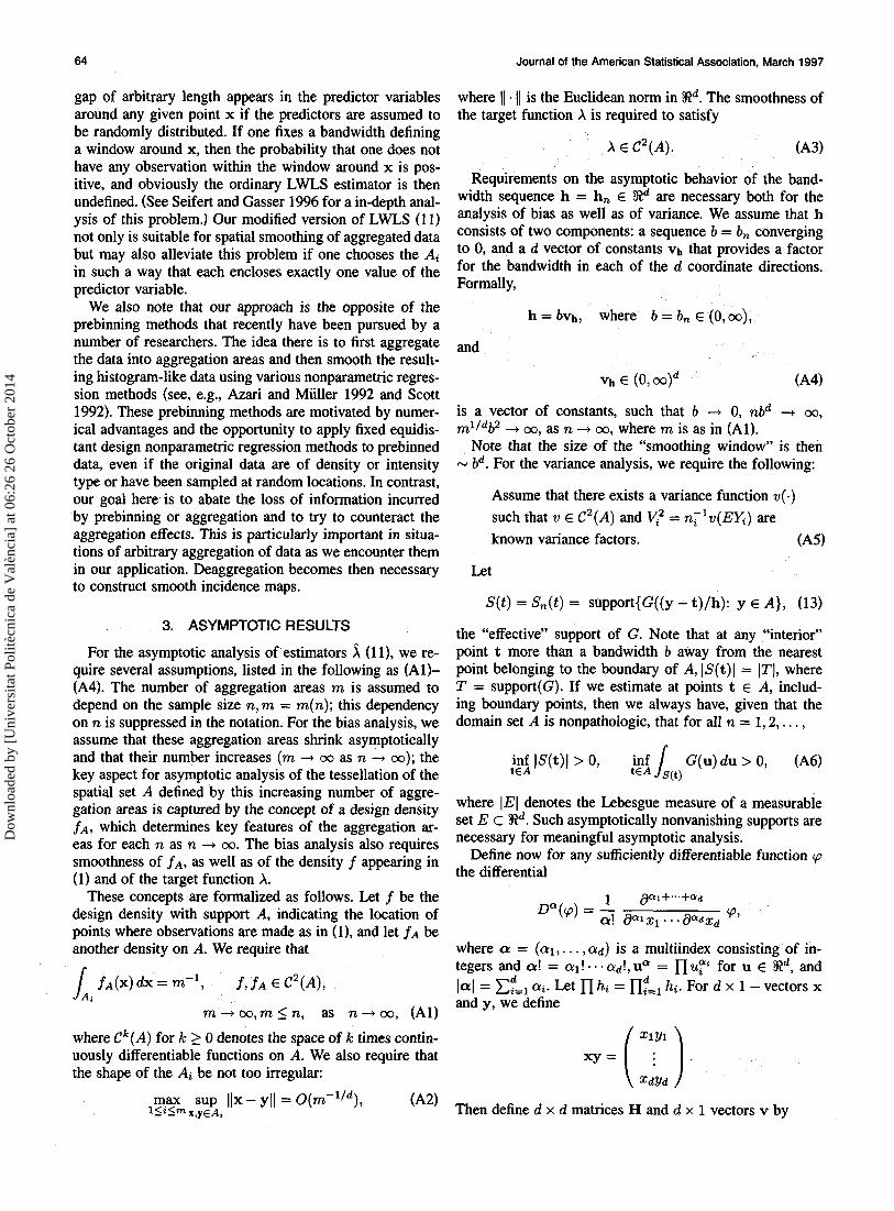
More details for the spatially aggregated count model are discussed in the next section. This model forms the basis for our application to AIDS incidence mapping where cases have been aggregated over zip code areas. In this applica- tion, N is the total number of AIDS cases, and n is the total number of population at risk on the domain A, cor- responding to the San Francisco County in our example. Figure 1 shows the division of San Francisco into zip code areas for which spatially aggregated AIDS incidence data are available, and Figure 2 displays the levels of incidence observed on each zip code area for the time period 1987- 89. Our aim is to produce a smooth intensity surface that will aid the study of spatiotemporal change as the epidemic spreads.

The remainder of the article is organized as follows: In Section 2 we introduce the proposed estimates for the target function X and list the necessary assumptions. We present the main asymptotic results regarding asymptotic mean squared error and asymptotic normality of these es- timators in Section 3. In Section 4 we discuss algorithmic details and give an application to geographically aggregated

Dow

nloa

ded

by [

Uni

vers

itat P

olitè

cnic

a de

Val

ènci

a] a

t 06:

26 2

6 O

ctob

er 2

014

Muller, Stadtmuller, and Tabnak: Spatial Smoothing 63

0

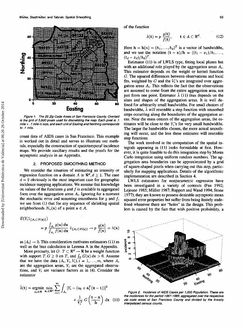
Easting Figure 1. The 25 Zip Code Areas of San Francisco Count$ Overlaid

is the grid of 5,600 pixels used for discretizing the map. Each pixel is . 1 mile x . 1 mile in size, and each unit of Easting and Northing corresponds to .1 mile.

count data of AIDS cases in San Francisco. This example is worked out in detail and serves to illustrate our meth- ods, especially the construction of spatiotemporal incidence maps. We provide auxiliary results and the proofs for the asymptotic analysis in an Appendix.

2. PROPOSED SMOOTHING METHOD We consider the situation of estimating an intensity or

regression function on a domain A in R d , d 2 1. The case d = 2 obviously is the most important case for geographic incidence mapping applications. We assume that knowledge on values of the functions g and f is available in aggregated form over the aggregation areas Ai. Ignoring for a moment the stochastic error and assuming smoothness for g and f , we see from (1) that for any sequence of shrinking spatial neighborhoods N,(x) of a point x E A,

as !Ail + 0. This consideration motivates estimators (1 1) as well as the bias calculation in Lemma A in the Appendix.

More precisely, let G: T c Rd + R be a weight function with support T, G 2 0 on T, and sT G(x) d x > 0. Assume that we have the data (Ai, Y,, Q) , i = 1,. . . ,m, where Ai are the aggregation areas, Y, are the aggregated observa- tions, and V, are variance factors as in (4). Consider the estimator

of the function

X(t) = p - t E A c Rd. f(tY (12)

Here h = h(n) = (Itl,. . . , hd)T is a vector of bandwidths, and we use the notation (t - x)/h = ((t l - q ) / h l , ...,

Estimator (11) is of LWLS type, fitting local planes but with an additional role played by the aggregation areas A,. This estimator depends on the weight or kernel function G. The squared differences between observations and local fits, weighted by G and the K’S are integrated over aggre- gation areas A,. This reflects the fact that the observations are assumed to come from the entire aggregation area, not just from one point. Estimator X (1 1) thus depends on the sizes and shapes of the aggregation areas. It is well de- fined for arbitrarily small bandwidths. For small choices of bandwidths, A will resemble a step function with smoothed steps occurring along the boundaries of the aggregation ar- eas. Near the mass centers of the aggregation areas, the es- timates will be close to the yZ’s for very small bandwidths. The larger the bandwidths chosen, the more actual smooth- ing will occur, and the less these estimates will resemble step functions.

The work involved in the computation of the spatial in- tegrals appearing in ( 1 1 ) looks formidable at first. How- ever, it is quite feasible to do this integration step by Monte Car10 integration using uniform random numbers. The ag- gregation area boundaries can be approximated by a grid of square-shaped pixels when carrying out this step, partic- ularly for mapping applications. Details of the algorithmic implementation are described in Section 4.

LWLS estimators for nonparametric regression have been investigated in a variety of contexts (Fan 1992; Lejeune 1985; Muller 1987; Ruppert and Wand 1994; Stone 1977); they are known to possess desirable asymptotic mean squared error properties but suffer from being finitely unde- fined whenever there are “holes” in the design. This prob- lem is caused by the fact that with positive probability, a

( t d - . d ) / W T .

(u

0

. . - .

A ( t ) = argmin min C [ y ~ - (a0 + a T ( x - t))12 Figure 2. Incidence of AIDS Cases per 1,000 Population. These are

the incidences for the period 1987- 1989, aggregated over the respective x - G ( T) d x (1 1) zip code areas of San Francisco County and divided by the linearly

1 t - x aoER alcSdi=1 \A ,

v,” interpolated census counts.

Dow

nloa

ded

by [

Uni

vers

itat P

olitè

cnic

a de

Val

ènci

a] a

t 06:

26 2

6 O

ctob

er 2

014

64 Journal of the American Statistical Association, March 1997

gap of arbitrary length appears in the predictor variables around any given point x if the predictors are assumed to be randomly distributed. If one fixes a bandwidth defining a window around x, then the probability that one does not have any observation within the window around x is pos- itive, and obviously the ordinary LWLS estimator is then undefined. (See Seifert and Gasser 1996 for a in-depth anal- ysis of this problem.) Our modified version of LWLS (1 1) not only is suitable for spatial smoothing of aggregated data but may also alleviate this problem if one chooses the Ai in such a way that each encloses exactly one value of the predictor variable.

We also note that our approach is the opposite of the prebinning methods that recently have been pursued by a number of researchers. The idea there is to first aggregate the data into aggregation areas and then smooth the result- ing histogram-like data using various nonparametric regres- sion methods (see, e.g., Azari and Muller 1992 and Scott 1992). These prebinning methods are motivated by numer- ical advantages and the opportunity to apply fixed equidis- tant design nonparametric regression methods to prebinned data, even if the original data are of density or intensity type or have been sampled at random locations. In contrast, our goal here is to abate the loss of information incurred by prebinning or aggregation and to try to counteract the aggregation effects. This is particularly important in situa- tions of arbitrary aggregation of data as we encounter them in our application. Deaggregation becomes then necessary to construct smooth incidence maps.

3. ASYMPTOTIC RESULTS

For the asymptotic analysis of estimators (1 l), we re- quire several assumptions, listed in the following as ( A l t (A4). The number of aggregation areas m is assumed to depend on the sample size n,m = m(n); this dependency on n is suppressed in the notation. For the bias analysis, we assume that these aggregation areas shrink asymptotically and that their number increases (m + 00 as n --$ 00); the key aspect for asymptotic analysis of the tessellation of the spatial set A defined by this increasing number of aggre- gation areas is captured by the concept of a design density f ~ , which determines key features of the aggregation ar- eas for each n as n + 00. The bias analysis also requires smoothness of f A , as well as of the density f appearing in (1) and of the target function A.

These concepts are formalized as follows. Let f be the design density with support A, indicating the location of points where observations are made as in (l), and let f~ be another density on A. We require that

fA(x ) dx = m-l, f, f A E c 2 ( A ) ,

m+oo,m<n, as n+m, (Al)

where @ ( A ) for k 2 0 denotes the space of k times contin- uously differentiable functions on A. We also require that the shape of the Ai be not too irregular:

where I ( . (1 is the Euclidean norm in W d . The smoothness of the target function X is required to satisfy

X E C2(A). (A3)

Requirements on the asymptotic behavior of the band- width sequence h = h, E Wd are necessary both for the analysis of bias as well as of variance. We assume that h consists of two components: a sequence b = b, converging to 0, and a d vector of constants Vh that provides a factor for the bandwidth in each of the d coordinate directions. Formally,

h = bvb, where b = b, E (0,00),

and

vh E ( O , O O ) d (A4)

is a vector of constants, such that b + 0, nbd --* 00,

m1Idb2 + 00, as n + 00, where m is as in (Al). Note that the size of the “smoothing window” is then

N bd. For the variance analysis, we require the following:

Assume that there exists a variance function v(-) such that v E C2(A) and v,’ = n;lv(EY,) are known variance factors. 645)

Let

S(t) = &(t) = support{G((y - t)/h): y E A } , (13)

the “effective” support of G. Note that at any “interior” point t more than a bandwidth b away from the nearest point belonging to the boundary of A, IS(t)l = ITI, where T = support(G). If we estimate at points t E A, includ- ing boundary points, then we always have, given that the domain set A is nonpathologic, that for all n = 1,2, . . . ,

where [El denotes the Lebesgue measure of a measurable set E c Rd. Such asymptotically nonvanishing supports are necessary for meaningful asymptotic analysis.

Define now for any sufficiently differentiable function cp the differential

where a = (al, . . . , a d ) is a multiindex consisting of in- tegers and a! = al!-.-ad!,uQ = nu:’ for u € Rd, and

= C;=, ai. Let n h i = n;=, hi. For d x 1 - vectors x and y, we define

max sup I I X - y11 = O(m-’Id), l< i<mx,yEA, (A2) Then define d x d matrices H and d x 1 vectors v by

Dow

nloa

ded

by [

Uni

vers

itat P

olitè

cnic

a de

Val

ènci

a] a

t 06:

26 2

6 O

ctob

er 2

014

Muller, Stadtmuller, and Tabnak: Spatial Smoothing 65

have limiting values for large n, even for boundary points, if the boundary of the total domain A is smooth.

We conclude this section with a result on asymptotic nor- mality.

Theorem 3.2. Under (AlHAS), if nb4+d + CO as n --$

00 for a constant <O 2 0, and if

Z ~ ~ F ~ , ( Z ) + o for M + 0O (20)

H = l,,, G(U)(UVh)(UVh)T du,

v = l(,) G(U)(UVh) du. (14)

For any t and n, define the “equivalent kernel function”

(15) z l > W K*(u) = G(u)[l- (UVh)TH-’V] Js(t) G(u)[1 - (UVh)TH-lV] du uniformly in 1 5 i 5 m, then

(nbd)1/2(i(t) - X ( t ) ) 4 and the “variance factor”

<A’2 C DaX(t) / K*(u)(uvh)adu, lal=2 W )

v2 (t) = v ( X ( t ) ) f A (t>/f(t)- (16)

Note that according to (Al), for any arbitrary t i f Ai, 1 L i 5 m,

772-l = J’, f ~ ( x ) dX = {fA(ti) + O(771-”d)}lAil, t

where

]Ail = m-’/{fA(ti) + O(m-’/d)} .

The connection of the variances v,“ (A5) of the obser- vations and the variance V2(.), which figures as variance factor in Theorem 3.1, is

(17)

This connection is used in the proof of the following central result (see the Appendix).

Under (AlHAG), S(t) denoting the ef- fective support of G as defined in (13),

m n = vyti) - (1 + o(m-’/d)}.

Theorem 3.2.

E(i(t)) = X(t) + b2 c DQA(t) lal=2

K*(U)(UVh)a du + o(b2) (18)

and

var(i(t)) = - v2(t) / K * ( u ) ~ ~ u + o (2) . (19) n n h i S(t) n n h t

Note that if G can be chosen in such a way that Js(,) G(u)ui du = 0, then v = 0 for v as in (14), and K* in (15) simplifies to K*(u) = G(u)/ J G(u) du. This is the case in the “interior” of A, away from the boundary, where IS(t)l = IT1 if T is compact. In the “boundary regions,” ker- nels K* (15) do depend on t and n for finite sample sizes and then correspond to “equivalent boundary kernels.” In- tegrals like Js(t) K * ( u ) ~ du and Js(,) K*(U)(UVh)a du Will

We remark that the uniform integrability condition (20) is satisfied if the yZ’s are identically distributed or if E)Y,12+6 < L < 00 for some L > 0 and some 6 > 0.

To conclude this section, we remark that estimators (1 1) can be viewed as special cases of a general class of estima- tors, which also includes classical LWLS estimators. These general estimators are defined as

where pn is a sequence of positive and finite measures and Y, is a random function. The case (1 1) is obtained when p, has Lebesgue density fn(t) = C 1~~ (t)/%2 and the random function is Y,(x) = y3 if x E A j . The case of classical LWLS based on scatterplot data (Xi, Y,) , i = 1,. . . , n is obtained when pn(x) = 6 ~ , (atom of size 1 placed at Xi) and Y,(x) = Y , if x = X,, Y,(x) = 0 otherwise.

4. FOR SAN FRANCISCO

We demonstrate our methods in the context of the spa- tially aggregated count model described in Section 1. Our aim is to describe the spatiotemporal spread of the AIDS epidemic in San Francisco. Counts of reported incident AIDS cases are available in spatially aggregated form for the m = 25 zip code areas of San Francisco County on a yearly basis for the years 1980-1992. Note that the Golden Gate Park, a narrow east-west-oriented rectangle at around Northing = 42 and Easting = 10 in the map of Figure 1, is not a zip code area, and thus no AIDS incidence is reported there. Accordingly, the entire Golden Gate Park area is con- sidered to be outside of the support set A, and the incidence there as everywhere else outside of A was set equal to 0. Note that, as can be seen from Figure 1, the resulting set A has a fairly complex shape.

CONSTRUCTION OF AIDS INCIDENCE MAPS Dow

nloa

ded

by [

Uni

vers

itat P

olitè

cnic

a de

Val

ènci

a] a

t 06:

26 2

6 O

ctob

er 2

014

66 Journal of the American Statistical Association, March 1997

In this application, the data Y, are (number of AIDS cases)/(number of residents) for the ith zip code area A, and the given time period. The density g is the density of AIDS occurrences over the domain, which is San Francisco County, and f is the density of the population as it spreads over the county or city area A. The total number of AIDS cases in a given time period is N, and the size of the pop- ulation for the same time period is n. Then

corresponds to the risk function for AIDS, in dependency on the location x E A. This function corresponds to the intensity of AIDS infections, adjusted for the population at risk.

We constructed the estimator (1 1) by evaluating the in- tegrals on the right side by Monte Carlo integration. We did this by generating 1,OOO pseudo-random numbers Xl with uniform distribution on A and then generating triplets (Xl, Wl, y2), where W’l = Y,, y2 = Y,/n,, if xl E A,, i = 1,. . . ,m,Z = 1,. . . , l ,OOO. Here we chose y2 according to (4) and (lo), combined with the Poisson-type approximation

We then smoothed these data by two-dimensional LWLS, fitting local planes as given in (1 1). Note that the quadrature error when approximating the integrals in (1 1) by the Monte Carlo integration method can be easily incorporated into the negligible remainder terms appearing in the asymptotic results (Theorems 3.1 and 3.2) by letting 1 + 00 sufficiently fast in comparison to n.

As a preliminary step, we discretized the entire map, in- cluding the zip code areas whose union constitutes the sup- port set A, into an equidistant grid of 70(north-south) x 80(east-west) square pixels, each with a sidelength of mile. We thus approximated each area by unions of such pixels. The zip code areas of San Francisco County are shown in Figure 1, with the grid of pixels overlaid. We then estimated the surface X at the midpoints of all 5,600 pixels and plotted the result.

V(Ey,) M EY, = y,.

We chose the weight function G as

. . .‘. . . . .

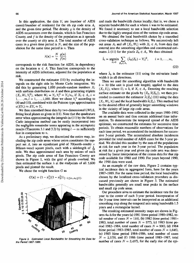
Figure 3. Estimated Local Bandwidths for Smoothing the Data for the Period 1987- 7 989.

and made the bandwidth choice locally; that is, we chose a separate bandwidth for each x where X was to be estimated. We found it necessary to use a local bandwidth selection due to the highly unequal sizes of the various zip code areas.

We obtained the local bandwidth choice by a smoothed cross-validation technique as follows. We successively left out areas Ai and all ( X l , Mrl) with Xl E Ai from data that entered into the smoothing algorithm and constructed esti- mates (1 1) for the pixels Zh E Ai. We thus obtained

(22)

where i b is the estimator (1 1) using the univariate band- width b in all directions.

Then we used the smoothing algorithm with bandwidth b = 30 (the unit is pixel side length), applied to the data (Xl, Ul), where Ul = 6, if Xl E A,. Denoting the resulting surface estimate on the pixels by (Zh, 6(&)), we then pro- ceeded to construct the estimator i(Zk) (1 1) using the data (Xl, Wl, &) and the local bandwidth &(&). This method led to the desired effect of generally larger smoothing windows in the vicinity of large zip code areas.

The available data were collected in the years 1980-1992 on an annual basis and thus contain additional time infor- mation. To demonstrate the temporal spread of the AIDS epidemic, we constructed the estimates for successive time periods. To obtain reasonable numbers of observations for each time period, we accumulated the incidencesfor succes- sive 3-year periods. The accumulated absolute incidences provided the total number of AIDS cases for the 3-year pe- riod. We divided this number by the sum of the populations at risk for each year in the 3-year period. The population at risk for a given year and given zip code area was deter- mined by linear interpolation of the census data for that zip code available for 1980 and 1990. For years beyond 1990, the 1990 data were used.

As an example of the raw data, Figure 2 contains typ- ical incidence data in aggregated form, here for the years 1987-1989. For the same time period, the local bandwidths chosen by the localized cross-validation procedure as dis- cussed previously are shown in Figure 3. The estimated bandwidths generally are small near peaks in the surface and small zip code areas.

Our procedure aims to estimate the incidence rate for the year in the center of each 3-year period. Incorporation of the 3-year time intervals can be interpreted as an additional smoothing step along the temporal axis using bandwidth 1.5 years and a rectangular kernel.

The resulting estimated intensity maps are shown in Fig- ures 4a-h for the years (a) 1981 (time period 1980-1982, to- tal number of cases N = 118), (b) 1982 (time period 1981- 1983, total number of cases N = 5771, (c) 1983 (time pe- riod 1982-1984, total number of cases N = goo), (d) 1984 (time period 1983-1985, total number of cases N = 1,646), (e) 1985 (time period 1984-1986, total number of cases N = 2,579), and (f) 1986 (time period 1985-1987, total number of cases N = 3,497), for the early rise of the epi-

Dow

nloa

ded

by [

Uni

vers

itat P

olitè

cnic

a de

Val

ènci

a] a

t 06:

26 2

6 O

ctob

er 2

014

Muller, Stadtmuller, and Tabnak: Spatial Smoothing 67

'.. . .. ... ....' . . $1'.

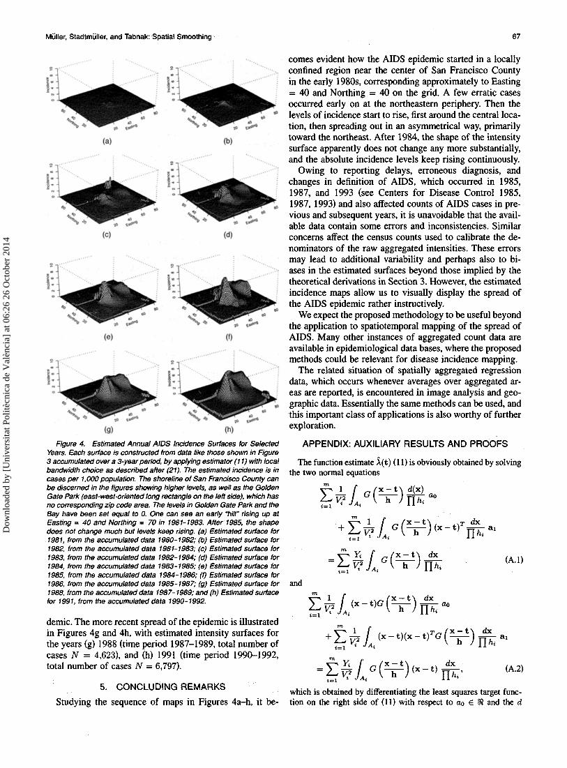
Figure 4. Estimated Annual AIDS Incidence Surfaces for Selected Years. Each surface is constructed from data like those shown in Figure 3 accumulated over a 3-year period, by applying estimator (1 1) with local bandwidth choice as described after (21). The estimated incidence is in cases per 1.000 population. The shoreline of San Francisco County can be discerned in the figures showing higher levels, as well as the Golden Gate Park (east- west-oriented long rectangle on the left side), which has no corresponding zip code area. The levels in Golden Gate Park and the Bay have been set equal to 0. One can see an early "hill" rising up at Easting = 40 and Northing = 70 in 1981-1983. After 1985, the shape does not change much but levels keep rising. (a) Estimated surface for 1981, from the accumulated data 1980-1982; (b) Estimated surface for 1982, from the accumulated data 198 1- 1983; (c) Estimated surface for 1983, from the accumulated data 1982- 1984; (d) Estimated surface for 1984, from the accumulated data 1983-1985; (e) Estimated surface for 1985, from the accumulated data 1984 - 1986; (0 Estimated surface for 1986, from the accumulated data 1985-1987; (9) Estimated surface for 1988, from the accumulated data 1987- 1989; and (h) Estimated surface for 1991, from the accumulated data 1990-1992.

demic. The more recent spread of the epidemic is illustrated in Figures 4g and 4h, with estimated intensity surfaces for the years (g) 1988 (time period 1987-1989, total number of cases N = 4,623), and (h) 1991 (time period 1990-1992, total number of cases N = 6,797).

5. CONCLUDING REMARKS Studying the sequence of maps in Figures 4a-h, it be-

comes evident how the AIDS epidemic started in a locally confined region near the center of San Francisco County in the early 1980s, corresponding approximately to Easting = 40 and Northing = 40 on the grid. A few erratic cases occurred early on at the northeastern periphery. Then the levels of incidence start to rise, first around the central loca- tion, then spreading out in an asymmetrical way, primarily toward the northeast. After 1984, the shape of the intensity surface apparently does not change any more substantially, and the absolute incidence levels keep rising continuously.

Owing to reporting delays, erroneous diagnosis, and changes in definition of AIDS, which occurred in 1985, 1987, and 1993 (see Centers for Disease Control 1985, 1987, 1993) and also affected counts of AIDS cases in pre- vious and subsequent years, it is unavoidable that the avail- able data contain some errors and inconsistencies. Similar concerns affect the census counts used to calibrate the de- nominators of the raw aggregated intensities. These errors may lead to additional variability and perhaps also to bi- ases in the estimated surfaces beyond those implied by the theoretical derivations in Section 3. However, the estimated incidence maps allow us to visually display the spread of the AIDS epidemic rather instructively.

We expect the proposed methodology to be useful beyond the application to spatiotemporal mapping of the spread of AIDS. Many other instances of aggregated count data are available in epidemiological data bases, where the proposed methods could be relevant for disease incidence mapping.

The related situation of spatially aggregated regression data, which occurs whenever averages over aggregated ar- eas are reported, is encountered in image analysis and geo- graphic data. Essentially the same methods can be used, and this important class of applications is also worthy of further exploration.

APPENDIX: AUXILIARY RESULTS AND PROOFS

The function estimate i(t) (1 1) is obviously obtained by solving the two normal equations

and

(A.1)

which is obtained by differentiating the least squares target func- tion on the right side of (11) with respect to uo E R and the d

Dow

nloa

ded

by [

Uni

vers

itat P

olitè

cnic

a de

Val

ènci

a] a

t 06:

26 2

6 O

ctob

er 2

014

68 Journal of the American Statistical Association, March 1997

2

= c V + ' Da ($ (t)) 1 G(u)(uvh)a components of a1 E Sd. The second equation (A.2) consists of d one-dimensional equations.

j = O lal=3 S(t) With 6, E (0, l}, i = 1,2, we have the following result.

Lemma A. Under (AlHA6). X (UVh) du + O(b3) . (A.5)

The integrals are over S(t), which in the limit will be a subset of

We immediately see from (A.4) that if we anticipate for a mo-

E(I1) = 0(1), (A.6)

m g(x)dx 1 G (q) { (x-t)1{61=1) + 1{61=0)} T = suppfi (GI. " S A , f dx A, a = l

T dx ment that {(x - t, l{62=1} + 1{62=0}} - n h, 2

= cb3+61+62 c Da(X(t)) L,,, G(U)(UVh)a then

1 4 = 3 E(Bo)T2(t) /,,,, G(u) du = (t) 1 G(u) du + O(b), J=o

T v2 S(t) x (uvh1{61=1} + 1{61=0))((uvh) 1{62=1) + 1{62=0})du (14.7)

(14.8)

Define for given integers v 2 0,6 E {0,1} and given functions Q the following quantities, which are scalars (6 = 0) or d vectors

>. (A*3) and thus + 4b2+61+62) + 0(~-1 /db61+62

E ( b ) = X ( t ) + O(b), Proof: Using Lipschitz continuity,

" a = 1 JA, f(x)dx 1 A, (-?;-) {(x - t)1{61=1) 4- 1{61=o})

./Alg(x)dx x - t which implies asymptotic unbiasedness of 60 for A(t) .

T dx (6 = 1): x {(x - t) 1{62=l) + 1{62=0}) - n ha

Dw5(p> = c D"(Q(t)) /,,, G(u)(uvh)a - ub)G(u)(uvhl{61=l) $. 1{61=0}) l a l e u

X {(UVh)T1{6=1) -I- 1{6=0)} du, (A.94 X ((uvh)Tl{62=1} + 1{62=o)) du + o(m -'Id)} * and d vectors (6 = 0) or d x d matrices (6 = 1)

The rest follows by a Taylor expansion of X around t. Note that an analogous result holds for other twice-

differentiable functions averaged over the Aa's. Applying Lemma A to the normal equations (A.l) and (A.2) and taking expectations on both sides, using (A.1HA.S) and (16). we have

1 X (UVh)T duE(g1)

X {(uvh)Tl{6=i> + l{a=o)}dU. (A.9b)

Assuming (A.61, we obtain more specifically from (A.4), ignoring terms of order o(b2):

(A.4)

and

- [DLO (h) - DO,I(V-~)E(&)]

Analogously, from (AS), noting that Do,o(X/V~) = X ( t ) 60 ,0(V-~) , and abbreviating DO,O = Do,o(l),D0,0 = Do,0(1), we obtain

X (UVh)T duE(4)

Dow

nloa

ded

by [

Uni

vers

itat P

olitè

cnic

a de

Val

ènci

a] a

t 06:

26 2

6 O

ctob

er 2

014

Muller, Stadtmuller, and Tabnak Spatial Smoothing 69

Note that with Observing that V-'(t)Di,o(A) = Do.i(V-2)VA(t)l

v-"t)6,,0(A) = Do,'(V-2)vA(t)l (A.17)

T a a V W ) = (at, W ) , . . . I A@))

and using basic differentiation rules, we obtain there exists a matrix M such that

D1,o (6) - A(t)Dl,o(V-') = V-'(t)D,,o(A), (A.12) A, = V-'(t)MVA(t)

and

and, noting that A is invertible, d1,o ($) - A(t)fil,o(V-') = V-z(t)fil,o(A)l (A.13) A = V 2 ( t ) M 1

D2,o ($) - A(t)Dz,o(V-') A - ~ A , = vx(t) .

= Dl,l(V-')VA(t) + V-'(t)Dz,o(A), (A.14) We find that with (A.14), (A.15),

Br = V-'(t) Dz,o(A) - !h! Dz,o(A)) Do.0

Do,, Do, (V-2)

( and

D z , o (h) - A(t)6z,o(v-2)

Do,o = D1,,(V-2)VA(t) + V-2(t)Dz,0(A). (A.15)

Inserting (A.12) and (A.13) into (A.11) and defining

(A. 18)

Dow

nloa

ded

by [

Uni

vers

itat P

olitè

cnic

a de

Val

ènci

a] a

t 06:

26 2

6 O

ctob

er 2

014

70 Journal of the American Statistical Association, March 1997

here the first factor is a d x d matrix, and the second factor is a d vector.

If G has certain symmetry properties, as can be assumed when estimating at an interior point of the domain A, then the terms lG(u)u: du drop out for odd powers j, and we obtain in this case

c = 0. (A.21)

From (A.16) and (A.20). we see that the earlier assumption (A.6) was justified. From (A.18), we obtain

E(&l(t)) = VX(t) + 6C + o(b), (A.22)

with the d vector C given as in (A.20).

Combining (A.22), (A.12), (A.141, and (A.17) with (A.10), we find

E(bo(t)) = X(t) + b2 Do,o Do,o

(A.23)

The proof of the following result is straightforward and thus is

Lemma B. For vectors v1 and v2 E %d and invertible d x d omitted.

matrices M, it holds that vT(M - VZV;)-~VZ = ~1 T 1 M- ~ 2 / ( l - vrM-'vz).

(A.24)

To apply (A.24), note that with H,v defined as in (14). we can rewrite (A.23) as

1 -l { .fG(U)(Uvh)adu - VT [. / G(u) du - vvT

G(u) du G(u) du E(bo(t) - X ( t ) ) = b2 c DaX(t) Irrl=2

- [/G(U)(Uvh)"(uvh)TH-lvd~] / [/G(u)du - vTH-'v]] + o(b2),

which implies (18). For a proof of (19). define vectors

Similar approximations yield

var(c, - vTE-lv,)

x - t dx and thus (19).

As for the asymptotic normality result (21), we use (A.25) to

and the d x d matrix

- - write b0 = C W,,X with given weights Win. We then show that

where asymptotic normality follows via the Lindeberg condition (cf. thm. 4.2 of Muller 1988).

x - t dx (x - t ) (x - t)T - n hi

to obtain

(A.25) !Received July 1995. Revised April 1996.1

REFERENCES Using Lemma A and similar arguments as in (17). the denomi- nator in (A.25) is seen to be

co - vTE-'vo Azari, A. S., and Muller, H. G. (1992). "Preaveraged Localized Orthogonal

Polynomial Estimators for Surface Smoothing and Partial Differentia- tion," Journal of the American Statistical Association, 87, 1005-1017.

1 Brillinger, D. R. (1990). "Spatial-Temporal Modeling of Spatially Aggre- = - /G(u) ( l - V2(t) (UVh)TH-lV)dU+O (n ha) ' gate Birth Data," Survey Methodology Journal, 16,255-269.

Dow

nloa

ded

by [

Uni

vers

itat P

olitè

cnic

a de

Val

ènci

a] a

t 06:

26 2

6 O

ctob

er 2

014

Muller, Stadtmuller, and Tabnak Spatial Smoothing 71

- D. R. (1994). “Examples of Scientific Problems and Data Analyses in Demography, Neurophysiology and Seismology,” Journal of Compu- tational and Graphical Statistics, 3, 1-22.

Carrat, F., and Valleron, A. J. (1992). “Epidemiologic Mapping Using the Kriging Method: Application to an Influenza-Like Illness Epidemic in France,” American Journal of Epidemiology, 135, 1293-1 300.

Centers for Disease Control (198% “Revision of the Case Definition of Acquired Immunodeficiency Syndrome for National Reporting-United States,” Mobidity and Mortality Weekly Report, 34, 373-375.

-(1987), “Revision of the CDC Surveillance Case Definition for Acquired Immunodeficiency Syndrome for National Reporting-United States,” Morbidity and Mortality Weekly Report, 36, 1-5. - (1992). “Revised Classification System for HIV Infection and Ex-

panded Surveillance Case Definition for AIDS Among Adolescents and Adults:’ Morbidity and Mortality Weekly Report, 41, 1-8.

Cressie, N. (1992). Statistics for Spatial Data, New York: Wiley. Fan, J. (1992), “Design-Adaptive Nonparametric Regression,” Journal of

the American Statistical Association, 87, 998-1004. Laslett. G. M. (1994). “Kriging and Splines: An Empirical Comparison

of Their Predictive Performance in Some Applications,” Journal of the American Statistical Association, 89, 391401.

Lejeune, M. (1 985), “Estimation Non-Paramitrique Par Noyaux: Rigression Polynomiale Mobile:’ Revue de Statistiques Appliquies, 33, 43-67.

McCullagh, P., and Nelder, J. A. (1991), Generalized Linear Models. Lon- don: Chapman and Hall.

Muller, H. G. (1987). “Weighted Local Regression and Kernel Methods for Nonparametric Curve Fitting,” Journal of the American Statistical Association, 82,231-238. - (1988), Nonparametric Regression Analysis of Longitudinal Data.

New York: Springer-Verlag. Ruppert, D., and Wand, M. (1994), “Multivariate Locally Weighted Least

Squares Regression,” The Annals of Statistics, 22, 1346-1370. Scott, D. (1992), Multivariate Density Estimation, New York: Wiley. Seifert, B., and Gasser, T. (1996). “Finite-Sample Variance of Local

Polynomials-Analysis and Solutions,” Journal of the American Sta- tistical Association, 91, 267-275.

Stone, C. J. ( I 977). “Consistent Nonparametric Regression,” The Annals of Statistics, 5, 505-545.

Szidarovsky, F., and Yakowitz, S. J. (1985). “A Comparison of Kriging with Nonparametric Regression Methods,” Journal of Multivariate Analysis, 16.21-53.

Dow

nloa

ded

by [

Uni

vers

itat P

olitè

cnic

a de

Val

ènci

a] a

t 06:

26 2

6 O

ctob

er 2

014