arX

iv:1

506.

0339

4v1

[cs.

IT]

10 J

un 2

015

Spatial Self-Interference Isolation for In-Band

Full-Duplex Wireless:

A Degrees-of-Freedom AnalysisEvan Everett and Ashutosh Sabharwal

Abstract

The challenge to in-band full-duplex wireless communication is managing self-interference. Many designs have

employed spatial isolation mechanisms, such as shielding or multi-antenna beamforming, to isolate the self-interference

wave from the receiver. Such spatial isolation methods are effective, but by confining the transmit and receive signals

to a subset of the available space, the full spatial resources of the channel be under-utilized, expending a cost that

may nullify the net benefit of operating in full-duplex mode.In this paper we leverage an antenna-theory-based

channel model to analyze the spatial degrees of freedom available to a full-duplex capable base station, and observe

that whether or not spatial isolation out-performs time-division (i.e. half-duplex) depends heavily on the geometric

distribution of scatterers. Unless the angular spread of the objects that scatter to the intended users is overlapped by

the spread of objects that backscatter to the base station, then spatial isolation outperforms time division, otherwise

time division may be optimal.

Index Terms

Full-duplex, antenna theory, self-interference, beamforming, massive multiple input multiple output (MIMO)

systems, degrees of freedom, physical channel models.

I. I NTRODUCTION

Currently deployed wireless communications equipment operates in half-duplex mode, meaning that transmission

and reception are orthogonalized either in time (time-division-duplex) or frequency (frequency-division-duplex).

Research in recent years [1]–[12] has investigated the possibility of wireless equipment operating in full-duplex

mode, meaning that transceiver will both transmit and receive at the same time and in the same spectrum. The

benefit of full-duplex is easy to see. Consider the communication scenario depicted in Figure 1. User 1 wishes to

transmit uplink data to a base station, and User 2 wishes to receive downlink data from the same base station. If the

base station is half-duplex, then it must either service theusers in orthogonal time slots or in orthogonal frequency

E. Everett and Ashu Sabharwal are with the Department of Electrical and Computer Engineering, Rice University, Houston, TX 77005, USA.

Email: evan.everett@rice.edu, ashu@rice.edu.

This paper was presented in part at the 2014 IEEE International Symposium on Information Theory.

This work was partially supported by National Science Foundation (NSF) Grants CNS 0923479, CNS 1012921, CNS 1161596 andNSF

Graduate Research Fellowship 0940902.

January 23, 2018 DRAFT

1

bands. If the base station can operate in full-duplex mode, then it can enhance spectral efficiency by servicing both

users simultaneously.1 The challenge to full-duplex communication, however, is that the base station transmitter

generates high-powered self-interference which potentially swamps its own receiver, precluding the reception of the

uplink message.

T1

User 1 (Uplink)

R1 T2

R2

User 2 (Downlink)

FD Base Station

S0Scatterers

Fig. 1: Three-node full-duplex model

For full-duplex to be feasible, the self-interference mustbe suppressed. The two main approaches to self-

interference suppression arecancellationandspatial isolation, and we now define each. Self-interference cancellation

is any technique which exploits the foreknowledge of the transmit signal by subtracting an estimate of the self-

interference from the received signal. The cancellation can be applied at digital baseband, at analog baseband, at

RF, or, as is most common, applied at a combination of these three domains [4]–[7], [11]. Spatial isolation is any

technique to spatially orthogonalize the self-interference and the signal-of-interest. Some spatial isolation techniques

studied in the literature are multi-antenna beamforming [1], [13], [14], directional antennas [15], shielding via

absorptive materials [16], and cross-polarization of transmit and receive antennas [10], [16]. The key differentiator

between cancellation and spatial isolation is that cancellation requires and exploits knowledge of the self-interference,

while spatial isolation does not. To our knowledge all full-duplex designs to date have required both cancellation and

spatial isolation in order for full-duplex to be feasible even at very short ranges (i.e.< 10 m).2 Moreover, because

cancellation performance is limited by transceiver impairments such as phase noise [17], spatial isolation often

accounts for an outsized portion of the overall self-interference suppression. For example, in the full-duplex design

of [16] which demonstrated full-duplex feasibility at WiFiranges, of the 95 dB of self-interference suppression

achieved,70 dB is due to spatial isolation, while only25 dB is due to cancellation. Therefore if full-duplex feasibility

is to be extended from WiFi-typical ranges to the ranges typical of femptocells or even larger cells, then excellent

1We assume that the pair of users are schedules for concurrentuplink and downlink on the basis of being hidden from one another, so that

interference from User 1 to User 2 will not be an issue.

2For example, see designs such as [5], [6], [10], [11], each ofwhich leverages cancellation techniques as well as at leastone spatial isolation

technique.

January 23, 2018 DRAFT

2

spatial isolation performance will be required, hence our focus is on spatial isolation in this paper.

In our previous work [16], we studied three passive techniques for spatial isolation: directional antennas, absorptive

shielding, and cross-polarization, and measured their performance in a prototype base station both in an anechoic

chamber that mimics free space, and in a reflective room. As expected, the techniques suppressed the self-interference

quite well (more than 70 dB) in the anechoic chamber, but in the reflective room the suppression was much less, (no

more than 45 dB), due the fact that the passive techniques such as directional antennas, absorptive shielding, and

cross-polarization operate primarily on the direct path between the transmit and receive antennas, and do little to

suppress paths that include an external scatterer. The direct-path limitation of passive spatial isolation mechanisms

raises the question of whether or not spatial isolation can be useful in a backscattering environment. Another class of

spatial isolation techniques called “active” or “channel aware” spatial isolation [18] can indeed suppress both direct

an backscattered self-interference. In particular, if multiple antennas are used and if the self-interference channel

response can be estimated, then the antenna patterns can be shaped adaptively to mitigate both direct-path and

backscattered self-interference, but this pattern shaping may consume spatial resources that could have otherwise

been leveraged for spatial multiplexing. Thus, there is a potential tradeoff in spatial self-interference isolation and

achievable degrees of freedom.

To appreciate the tradeoff, consider the example illustrated in Figure 1. The direct path from the base station

transmitter,T2, to its receiverR1, can be passively suppressed by shielding the receiver fromthe transmitter as

shown in [16], but there will also be self-interference due to transmit signal backscattered from objects near the

base station (depicted by gray blocks in Figure 1). The self-interference caused by scattererS0, for example, in

Figure 1 could be avoided by creating a null in the direction of S0. However losing access to that scatterer could

lead to a less rich scattering environment, diminishing thespatial degrees of freedom of the uplink or downlink.

Moreover, creating the null consumes antenna resources at the base station that could have been leveraged for

spatial multiplexing to the downlink user, diminishing thespatial degrees of freedom the downlink. This example

leads us to pose the following question.

Question: Under what scattering conditions can spatial isolation beleveraged in full-duplex to provide a degree-

of-freedom gain over half-duplex? More specifically, givena constraint on thesize of the antenna arrays at the

base station and at the User 1 and User 2 devices, and given a characterization of thespatial distributionof the

scatterers in the environment, what is the uplink/downlinkdegree-of-freedom region when the only self-interference

mitigation strategy is spatial isolation?

Modeling Approach: To answer the above question we leverage the antenna-theory-based channel model devel-

oped by Poon, Broderson, and Tse in [19]–[21], which we will label the “PBT” model. In the PBT model, instead

of constraining thenumberof antennas, thesizeof the array is constrained. Furthermore, instead of considering a

channel matrix drawn from a probability distribution, a channel transfer function which depends on the geometric

position of the scatterers relative to the arrays is considered.

Contribution: We extend the PBT model to the three-node full-duplex topology of Figure 1, and derive the degree-

of-freedom regionDFD, i.e. the set of all achievable uplink/downlink degree-of-freedom tuples. By comparingDFD to

January 23, 2018 DRAFT

3

DHD, the degree-of-freedom region achieved by time-division half-duplex, we observe that full-duplex outperforms

half-duplex, i.e.DHD ⊂ DFD, in the following two scenarios.

1) When the base station arrays are larger than the corresponding user arrays, the base station has a larger signal

space than is needed for spatial multiplexing and can leverage the extra signal dimensions to form beams that

avoid self-interference (i.e. self zero-forcing).

2) More interestingly, when the forward scattering intervals and the backscattering intervals are not completely

overlapped, the base station can avoid self-interference by signaling in the directions that scatter to the intended

receiver, but do not backscatter to the base-station receiver. Moreover the base station can also signal in

directions thatdo cause self-interference, but ensure that the generated self-interference is incident on the

base-station receiver only in directions in which uplink signal isnot incident on the base-station receiver, i.e.

signal such that the self-interference and uplink signal are spatially orthogonal.

Organization of the Paper: Section II specifies the system model: we begin with an overview of the PBT model

in Section II-A and then in Section II-B apply the model to thescenario of a full-duplex base station with uplink and

downlink flows. Section III gives the main analysis of the paper, the derivation of the degrees-of-freedom region.

We start Section III by stating the theorem which characterizes the degrees of freedom region and then give the

achievability and converse arguments in Sections III-A andIII-B, respectively. In Section IV we assess the impact

of the degrees-of-freedom result on the design and deployment of full-duplex base stations, and we conclude in

Section V.

II. SYSTEM MODEL

We now give a brief overview of the PBT channel model presented in [19]. We then extend the PBT model to

the case of the three-node full-duplex topology of Figure 1,and define the required mathematical formalism that

will ease the degrees-of-freedom analysis in the sequel.

A. Overview of the PBT Model

The PBT channel model considers a wireless communication link between a transmitter equipped with a unipo-

larized continuous linear array of length2LT and a receiver with a similar array of length2LR. The authors observe

that there are two key domains: thearray domain, which describes the current distribution on the arrays, and the

wavevector domainwhich describes radiated and received field patterns. Motivated by channel measurements which

show that the angles of departure and the angles of arrival ofthe physical paths from a transmitter to a receiver tend

to be concentrated within a handful of angular clusters [22]–[25], the authors focus on the union of the clusters of

departure angles from the transmit array, denotedΘT , and the union of the clusters of arrival angles to the receive

array,ΘR . Because a linear array aligned to thez-axis array can only resolve thez-component, the intervals of

interest areΨT = cos θ : θ ∈ ΘT andΨR = cos θ : θ ∈ ΘR. In [19], it is shown from the first principles

of Maxwell’s equations that an array of length2LT has a resolution of1/(2LT ) over the intervalΨT , so that the

January 23, 2018 DRAFT

4

dimension of the transmit signal space of radiated field patterns is2LT |ΨT |. Likewise the dimension of the receive

signal space is2LR|ΨR|, so that the degrees of freedom of the communication link is

dP2P = min 2LT |ΨT |, 2LR|ΨR| . (1)

B. Extension of PBT Model to Three-Node Full-Duplex

ΘT11

ΘR11

ΘT12ΘR12

ΘT22

ΘR22

T1

T2R1

R2

2LR12LT2

2LR22LT1

FD Base Station

User 1 (Uplink) User 2 (Downlink)

Fig. 2: Clustered scattering. Only one cluster for each transmit receive pair is shown to prevent clutter.

Now we extend the PBT channel model in [19], which considers apoint-to-point topology, to the three-node

full-duplex topology of Figure 1. LetFlow1 denote the uplink flow from User 1 to the base station, and letT1

denote User 1’s transmitter andR1 denote the base station’s receiver, as is illustrated in Figure 1. Similarly, let

Flow2 denote the downlink flow from the base station to User 2, and let T2 denote the base station’s transmitter

andR2 denote User 2’s receiver.

As in [19], we consider continuous linear arrays of infinitely many infinitesimally small unipolarized antenna

elements. Each of the two transmittersTj, j = 1, 2, is equipped with a linear array of length2LTj, and each

receiver,Ri, i = 1, 2, is equipped with a linear array of length2LRi. The lengthsLTj

andLRiare normalized

by the wavelength of the carrier, and thus are unitless quantities. For each array, define a local coordinate system

with origin at the midpoint of the array andz-axis aligned along the lengths of the array. LetθTj∈ [0, π) denote

the elevation angle relative to theTj array, and letθRidenote the elevation angle relative to theRi array. We will

see in the following that the field pattern radiated from theTj array will depend onθTjonly throughcos θTj

. Thus

let tj ≡ cos θTj∈ (−1, 1], and likewiseτi ≡ cos θRi

∈ (−1, 1]. Denote the current distribution on theTj array as

xj(pj), wherepj ∈ [−LTj, LTj

] is the position along the lengths of the array, andxj : [−LTj, LTj

] → C gives

the magnitude and phase of the current. The current distribution, xj(pj), is the transmit signal controlled byTj,

which we constrain to be square integrable. Likewise we denote the received current distribution on theRi array

asyi(qi), qi ∈ [−LRi, LRi

].

January 23, 2018 DRAFT

5

The current signal received by the base station receiver,R1, at a pointq1 ∈ [−LR2, LR2

] along its array is given

by

y1(q1) =

∫ LT1

−LT1

C11(q1, p1)x1(p1)dp1 +

∫ LT2

−LT2

C12(q1, p2)x2(p2)dp2 + z1(q1), q1 ∈ [−LR1, LR1

] (2)

wherez1(q1), q1 ∈ [−LR1, LR1

] is the noise along theR1 array. The channel response integral kernel,Cij(qi, pj),

gives the current excited at a pointqi on theRi receive array due to a current at the pointpj on theTj transmit

array. Note that the first term in (2) gives the received uplink signal-of-interest, while the second term gives the

self-interference generated by the base stations transmission. We assume that the mobile users are out of range of

each other, such that there is no channel fromT1 to R2. ThusR2’s received signal at a pointq2 ∈ [−LR2, LR2

] is

y2(q2) =

∫ LT2

−LT2

C22(q2, p2)x2(p2)dp2 + z2(q2), q2 ∈ [−LR2, LR2

]. (3)

As in [19], the channel response kernel,Cij(·, ·), from transmitterTj to receiverRi is composed of a transmit

array responseATj(·, ·), a scattering responseHij(·, ·), and a receive array responseARi

(·, ·). The channel response

kernel is given by

Cij(q, p) =

∫∫

ARi(q, κ)Hij(κ, k)ATj

(k, p)dkdκ, (4)

wherek is a unit vector that gives the direction of propagation fromthe transmitter array, andκ is a unit vector that

gives the direction of a propagation to the receiver array. The transmit array response kernel,ATj(k, p), maps the

current distribution along theTj array (a function ofp) to the field pattern radiated fromTj (a function of direction

of departure,k). The scattering response kernel,Hij(κ, k), maps the fields radiated fromTj in direction k to the

fields incident onRi at directionκ. The receive array response,ARi(q, κ), maps the field pattern incident onRi

(a function of direction of arrival,κ) to the current distribution excited on theRi array (a function of positionq),

which is the received signal.

C. Array Responses

In [19], the transmit array response for a linear array is derived from the first principles of Maxwell’s equations

and shown to be

ATj(k, p) = ATj

(cos θTj, p) = e−i2πp cos θTj , p ∈

[

−LTj, LTj

]

,

whereθTj∈ [0, π) is the elevation angle relative to theTj array. Due to the symmetry of the array (aligned to the

z-axis) its radiation pattern is symmetric with respect to the azimuth angle and only depends on the elevation angle

θTjthroughcos θTj

. For notational convenience lett ≡ cos θTj∈ [−1, 1], so that we can simplify the transmit array

response kernel to

ATj(t, p) = e−i2πpt, t ∈ [−1, 1], p ∈

[

−LTj, LTj

]

. (5)

By reciprocity, the receive array response kernel,ARi(q, κ), is

ARi(q, τ) = ei2πqτ , τ ∈ [−1, 1], q ∈ [−LRi

, LRi] , (6)

January 23, 2018 DRAFT

6

whereτ ≡ cos θRi∈ [−1, 1] is the cosine of the elevation angle relative to theRi array. Note that the transmit and

receive array response kernels are identical to the kernelsof the Fourier transform and inverse Fourier transform,

respectively, a relationship we will further explore in Section II-E.

D. Scattering Responses

The scattering response kernel,Hij(κ, k), gives the amplitude and phase of the path departing fromTj in

direction k and arriving atRi in directionκ. Since we are considering linear arrays which only resolve the cosine

of the elevation angle, we can considerHij(τ, t) which gives the superposition of the amplitude and phase of all

paths emanating fromTj with an elevation angle whose cosine ist and arriving atRi at an elevation angle whose

cosine isτ . As is done in [19], motivated by measurements showing that scattering paths are clustered with respect

to the transmitter and receiver, we adopt a model that focuses on theboundaryof the scattering clusters rather than

the discrete paths themselves, as illustrated in Figure 2.

LetΘ(k)Tij

denote the angle subtended at transmitterTj by thekth cluster that scatters toRi, and letΘTij=

⋃

k Θ(k)Tij

be the total transmit scattering interval fromTj to Ri. The scattering intervalΘTijcan be thought of as the set of

directions that when illuminated byTj scatters energy toRi. In Figure 2, to avoid clutter we illustrate the case in

which Θ(k)Tij

is a single contiguous angular interval, but in general the interval will be non-contiguous and consist

of several individual clusters. Similarly letΘ(k)Rij

denote the corresponding solid angle subtended atRi by thekth

cluster illuminated byTj, and letΘRij=

⋃

k Θ(k)Rij

be set of directions from which energy is incident onRi from

Tj.

Thus, we see in Figure 2 that from the point-of-view of the base-station transmitter,T2, ΘT22is the angular

interval over which it can radiate signals that will couple to the intended downlink receiver,R2, while ΘT12is the

interval in which radiated signals will scatter back to the base station receiver,R1, as self-interference. Likewise,

from the point-of-view of the base station receiver,R1, ΘR11is the interval over which it may receive signals

from the User 1 transmitter,T1, while ΘR12is the interval in which self-interference may be present. Clearly, the

extent to which the interference intervals and the signal-of-interest intervals overlap will have a major impact on

the degrees of freedom of the network. Because linear arrayscan only resolve the cosine of the elevation angle

t ≡ cos θ, let us denote the “effective” scattering interval as

ΨTij≡

t : arccos(t) ∈ ΘTij

⊂ [−1, 1].

Likewise for the receiver side we denote the effective scattering intervals as

ΨRij≡

τ : arccos(τ) ∈ ΘRij

⊂ [−1, 1].

Define the size of the transmit and receive scattering intervals as

|ΨTij| =

∫

ΨTij

t dt, |ΨRij| =

∫

ΨRij

τ dτ. (7)

As in [19], we assume the following characteristics of the scattering responses:

January 23, 2018 DRAFT

7

1) Hij(τ, t) 6= 0 only if (τ, t) ∈ ΨRij×ΨTij

.

2)∫

||Hij(τ, t)||dt 6= 0 ∀ τ ∈ ΨRij.

3)∫

||Hij(τ, t)||dτ 6= 0 ∀ t ∈ ΨTij.

4) The point spectrum ofHij(·, ·), excluding0, is infinite.

5) Hij(·, ·) is Lebesgue measurable, that is∫ 1

−1

∫ 1

−1|Hij(τ, t)|

2 dτ dt < ∞.

The first condition means that the scattering response is zero unless the angle of arrival and angle of departure

both lie within their respective scattering intervals. Thesecond condition means that in any direction of departure,

t ∈ ΨTij, from Tj there exists at least one path to receiverRi. Similarly, the third condition implies that in any

direction of arrival,τ ∈ ΨRij, to Ri there exists at least one path fromTj. The fourth condition means that there

are many paths from the transmitter to the receiver within the scattering intervals, so that the number of propagation

paths that can be resolved within the scattering intervals is limited by the length of the arrays and not by the number

of paths. The final condition aids our analysis by ensuring the corresponding integral operator is compact, but is

also physically justified assumption since one could argue for the stricter assumption∫ 1

−1

∫ 1

−1 |Hij(τ, t)|2 dτ dt ≤ 1,

since no more energy can be scattered than is transmitted.

E. Hilbert Space of Wave-vectors

We can now write the original input-output relation given in(2) and (3) as

y1(q) =

∫

ΨR11

AR1(q, τ)

∫

ΨT11

H11(τ, t)

∫ LT1

−LT1

AT1(t, p)x1(p) dτ dt dp

+

∫

ΨR12

AR1(q, τ)

∫

ΨT12

H12(τ, t)

∫ LT2

−LT2

AT2(t, p)x2(p) dτ dt dp+ z1(q), (8)

y2(q) =

∫

ΨR22

AR2(q, τ)

∫

ΨT22

H22(τ, t)

∫ LT2

−LT2

AT2(t, p)x2(p) dτ dt dp+ z2(q). (9)

The channel model of (8) and (9) is expressed in thearray domain, that is the transmit and receive signals are

expressed as the current distributions excited along the array. Just as one can simplify a signal processing problem

by leveraging the Fourier integral to transform from the time domain to the frequency domain, we can leverage the

transmit and receive array responses to transform the problem from the array domain to thewave-vectordomain. In

other words, we can express the transmit and receive signalsas field distributions over direction rather than current

distributions over position along the array. In fact, for our case of the unipolarized linear array, the transmit and

receive array responsesare the Fourier and inverse-Fourier integral kernels, respectively.

Let Tj be the space of all field distributions that transmitterTj ’s array of lengthLTjcan radiate towards the

available scattering clusters,ΨTjj∪ ΨTij

(both signal-of-interest and self-interference). In the vernacular of [19],

Tj is the space of field distributions array-limited toLTjand wavevector-limited toΨTjj

∪ ΨTij. To be precise,

defineTj to be the Hilbert space of all square-integrable functionsXj : ΨTjj∪ΨTij

→ C, that can be expressed as

Xj(t) =

∫ LTj

−LTj

ATj(t, p)xj(p) dp, t ∈ ΨTjj

∪ΨTij

January 23, 2018 DRAFT

8

for somexj(p), p ∈ [−LTj, LTj

]. The inner product between two member functions,Uj, Vj ∈ Tj , is the usual

inner product

〈Uj , Vj〉 =

∫

ΨTjj∪ΨTij

Uj(t)V∗j (t) dt.

Likewise letRi be the space of field distributions that can be incident on receiverRi from the available scattering

clusters,ΨRii∪ ΨRij

, and resolved by an array of lengthLRi. More precisely,Ri is the Hilbert space of all

square-integrable functionsYi : ΨRii∪ΨRij

→ C, that can be expressed as

Yi(τ) =

∫ LRi

−LRi

A∗Ri(q, τ)yi(q) dq, τ ∈ ΨRii

∪ΨRij

for someyi(q), q ∈ [−LRi, LRi

], with the usual inner product. From [19], we know that the dimension of these

array-limited and wavevector-limited transmit and receive spaces are, respectively,

dim Tj = 2LTj|ΨTjj

∪ΨTij|, and (10)

dimRi = 2LRi|ΨRii

∪ΨRij|. (11)

We can think of the scattering integrals in (8) and (9) as operators mapping from one Hilbert space to another.

Define the operatorHij : Tj → Ri by

(HijXj)(τ) =

∫

ΨTij∪ΨTjj

Hij(τ, t)Xj(t) dt, τ ∈ ΨRij∪ΨRii

. (12)

We can now write the channel model of (8) and (8) in the wave-vector domain as

Y1 = H11X1 + H12X2 + Z2, (13)

Y2 = H22X2 + Z2, (14)

whereXj ∈ Rj , for j = 1, 2 andYi, Zi ∈ Ri for i = 1, 2.

The following lemma states key properties of the scatteringoperators in (13-14), that we will leverage in our

analysis.

Lemma 1:The scattering operatorsHij , (i, j) ∈ (1, 1), (2, 2), (1, 2) have the following properties:

1) Hij : Tj → Ri is a compact operator

2) dimR(Hij) = dimN(Hij)⊥ = 2minLTj

|ΨTij|, LRi

|ΨRij|

3) There exists a singular system

σ(k)ij , U

(k)ij , V

(k)ij

∞

k=1for operatorHij , and a singular valueσ(k)

ij is nonzero

if and only if k ≤ 2minLTj|ΨTij

|, LRi|ΨRij

|.

Proof: Property 1 holds because we have assumed thatHij(·, ·), the kernel of integral operatorHij , is square

integrable, and any integral operator with a square integrable kernel is compact (see Theorem 8.8 of [26]). Property

2 is just a restatement of the main result of [19]. Property 3 follows from the first two properties: The compactness

of Hij , established in Property 1, implies the existence of a singular system, since there exists a singular system for

any compact operator (see Section 16.1 of [26]). Property 2 implies that only the first2minLTj|ΨTij

|, LRi|ΨRij

|

of the singular values will be nonzero, since theU(k)ij corresponding to nonzero singular values form a basis for

January 23, 2018 DRAFT

9

R(Hij), which has dimension2minLTj|ΨTij

|, LRi|ΨRij

| . See Lemma 5 in Appendix B for a description of

the properties of singular systems for compact operators, or see Section 2.2 of [27] or Section 16.1 of [26] for a

thorough treatment.

III. SPATIAL DEGREES-OF-FREEDOM ANALYSIS

We now give the main result of the paper: a characterization of the spatial degrees-of-freedom region for the

PBT channel model applied full-duplex base station with uplink and downlink flows.

Theorem 1:Let d1 andd2 be the spatial degrees of freedom ofFlow1 andFlow2 respectively. The spatial degrees-

of-freedom region,DFD, of the three-node full-duplex channel is the convex hull ofall spatial degrees-of-freedom

tuples,(d1, d2), satisfying

d1 ≤ dmax

1 = 2min(LT1|ΨT11

|, LR1|ΨR11

|), (15)

d2 ≤ dmax

2 = 2min(LT2|ΨT22

|, LR2|ΨR22

|), (16)

d1 + d2 ≤ dmax

sum = 2LT2|ΨT22

\ΨT12|+ 2LR1

|ΨR11\ΨR12

|+ 2max(LT2|ΨT12

|, LR1|ΨR12

|). (17)

The degrees-of-freedom region characterized by Theorem 1DFD is the pentagon-shaped region shown in Figure 3.

The achievability part of Theorem 1 is given in Section III-Aand the converse is given in Section III-B.

dmaxsum − dmax

1 dmax1

dmaxsum − dmax

2

dmax2

d1 + d2 = dmaxsum

(d′′1 , d′′2 )

(d′1, d′2)

d1

d2

Fig. 3: degrees-of-freedom region,DFD

A. Achievability

We establish achievability ofDFD by way of two lemmas. The first lemma shows the achievability of two specific

spatial degrees-of-freedom tuples, and the second lemma shows that these tuples are indeed the corner points of

DFD.

Lemma 2:The spatial degree-of-freedom tuples(d′1, d′2) and (d′′1 , d

′′2 ) are achievable, where

January 23, 2018 DRAFT

10

d′1 =min 2LT1|ΨT11

|, 2LR1|ΨR11

| , (18)

d′2 =min dT2, 2LR2

|ΨR22| 1(LT1

|ΨT11| ≥ LR1

|ΨR11|)

+ min δT2, 2LR2

|ΨR22| 1(LT1

|ΨT11| < LR1

|ΨR11|), (19)

d′′1 =min 2LT1|ΨT11

|, dR1 1(LR2

|ΨR22| ≥ LT2

|ΨT22|)

+ min 2LT1|ΨT11

|, δR1 1(LR2

|ΨR22| < LT2

|ΨT22|), (20)

d′′2 =min 2LT2|ΨT22

|, 2LR2|ΨR22

| , (21)

with dT2, δT2

, dR1, andδR1

given in (22-25), and where1(arg) is an indicator function that evaluates to one if the

argument it true, and otherwise evaluates to zero.

dT2= 2LT2

|ΨT22\ΨT12

|+ 2min

LT2|ΨT22

∩ΨT12|, (LT2

|ΨT12| − LR1

|ΨR12|)+ + LR1

|ΨR12\ΨR11

|

(22)

δT2= 2LT2

|ΨT22\ΨT12

|+ 2min

LT2|ΨT22

∩ΨT12|, LT2

|ΨT12|

−[

LT1|ΨT11

| −(

LR1|ΨR11

\ΨR12|+ (LR1

|ΨR12| − LT2

|ΨT12|)+

)]

(23)

dR1= 2LR1

|ΨR11\ΨR12

|+ 2min

LR1|ΨR11

∩ΨR12|, (LR1

|ΨR12| − LT2

|ΨT12|)+ + LT2

|ΨT12\ΨT22

|

(24)

δR1= 2LR1

|ΨR11\ΨR12

|+ 2min

LR1|ΩR11

∩ΨR12|, LR1

|ΨR12|

−[

LR2|ΨR22

| −(

LT2|ΨT22

\ΨT12|+ (LT2

|ΨT12| − LR1

|ΨR12|)+

)]

(25)

Proof: Due to the symmetry of the problem, it suffices to demonstrateachievability of only the first spatial

degree-of-freedom pair in Lemma 2, (d′1, d′2), as the second pair, (d′′1 , d

′′2 ), follows from the symmetry. Thus we

seek to prove the achievability of the tuple (d′1, d′2) given in (18-19). We will show achievability of (d′1, d

′2) in the

case whereLT1|ΨT11

| ≥ LR1|ΨR11

|, for which

d′1 = 2LR1|ΨR11

|, (26)

d′2 = min dT2, 2LR2

|ΨR22| , (27)

where

dT2= 2LT2

|ΨT22\ΨT12

|+min

2LT2|ΨT22

∩ΨT12|,

2(LT2|ΨT12

| − LR1|ΨR12

|)+ + 2LR1|ΨR12

\ΨR11|

. (28)

Achievability of (d′1, d′2) in the LT1

|ΨT11| < LR1

|ΨR11| case is analogous. We now begin the steps to show

achievability of (26-27).

January 23, 2018 DRAFT

11

1) Defining Key Subspaces:We first define some subspaces of the transmit and receive wave-vector spaces (T1,

T2, R1, andR2) that will be crucial in demonstrating achievability.

Subspaces of T2: Recall thatT2 is the space of all field distributions that can be radiated bythe base station

transmitter,T2, in the direction of the scatterer intervals,ΨT22∪ΨT12

, (both signal-of-interest and self-interference).

Let T22\12 ⊆ T2 be the subspace of field distributions that can be transmitted by T2, which are nonzero only in the

intervalΨT22\ΨT12

,

T22\12 ≡ spanX2 ∈ T2 : X2(t) = 0 ∀ t ∈ ΨT12. (29)

More intuitively, T22\12 is the space of transmissions from the base station which couple only to the intended

downlink user, and do not couple back to the base station receiver as self-interference. Similarly letT12 ⊆ T2 the

subspace of functions that are only nonzero in the intervalΨT12,

T12 ≡ spanX2 ∈ T2 : X2(t) = 0 ∀ t /∈ ΨT12, (30)

that is, the space of base station transmissions whichdo couple to the base station receiver as self-interference.

Finally, letT22∩12 ⊆ T12 ⊆ T2 be the subspace of field distributions that are nonzero only in the intervalΨT22∩ΨT12

,

T22∩12 ≡ spanX2 ∈ T2 : X2(t) = 0 ∀ t /∈ ΨT22∩ΨT12

, (31)

the space of base station transmission which coupleboth to the downlink user and to the base station receiver.

From the result of [19], we know that the dimension of each of these transmit subspaces ofT1 is as follows:

dim T12 = 2LT2|ΨT12

|, (32)

dim T22\12 = 2LT2|ΨT22

\ΨT12|, (33)

dim T22∩12 = 2LT2|ΨT22

∩ΨT12|. (34)

One can check thatT12 andT22\12 are constructed such that they form anorthogonal direct sumfor spaceT2, a

relation we notate as

T2 = T12 ⊕ T22\12. (35)

By orthogonal direct sumwe mean that anyX2 ∈ T2 can be written asX2 = X2Orth+X2Int , for someX2Orth

∈ T22\12

and X2Int ∈ T12, such thatX2Orth⊥ X2Int . By the construction ofT22\12, H12X2Orth

= 0, sinceH12(τ, t) = 0

∀ t /∈ ΨT12and X2Orth

∈ T22\12 implies X2Orth(t) = 0 ∀ t ∈ ΨT12

. In other words,X2Orth∈ T22\12 is zero

everywhere the integral kernelH12(τ, t) is nonzero. Thus any transmitted field distribution that lies in the subspace

T22\12 will not present any interference toR2.

Subspaces of T1: Recall thatT1 is the space of all field distributions that can be radiated bythe uplink user

transmitter,T1, towards the available scatterers. LetT11 ⊆ T1 be the subspace of field distributions that can be

transmitted byT1’s continuous linear array of lengthLT1which are nonzero only in the intervalΨT11

,3 more

3Note thatT11 = T1, since we have assumedΨT21= ∅. AlthoughT11 is thus redundant, we define it for notational consistency

January 23, 2018 DRAFT

12

precisely

T11 ≡ spanX1 ∈ T1 : X1(t) = 0 ∀ t /∈ ΨT11. (36)

More intuitively, T11 is the space of transmissions from the uplink user which willcouple to the base station

receiver. From the result of [19], we know that

dim T11 = 2LT1|ΨT11

|. (37)

Subspaces of R1: Recall thatR1 is the space of all incident field distributions that can be resolved by the base

station receiver,R1. Let R12 ⊆ R1 to be the subspace of received field distributions which are nonzero only for

τ ∈ ΨR12, that is

R12 ≡ spanY1 ∈ R1 : Y1(τ) = 0 ∀ τ /∈ ΨR12. (38)

Less formally,R12 is the space of receptions at the base station which could have emanated from the base stations

own transmitter. SimilarlyR12\11 ⊆ R12 ⊆ R1 be the subspace of received field distributions that are onlynonzero

for τ ∈ ΨR12\ΨR11

,

R12\11 ≡ spanY1 ∈ R1 : Y1(τ) = 0 ∀ τ ∈ ΨR11. (39)

Less formally,R12\11 is the space of receptions at the base station which could have emanated from the base

station transmitter, but could not have emanated from the uplink user. Finally, defineR11 ⊆ R1 to be the subspace

of received field distributions that are nonzero only forτ ∈ ΨR11,

R11 ≡ spanY1 ∈ R1 : Y1(τ) = 0 ∀ τ /∈ ΨR11, (40)

the space of base station receptions which could have emanated from the intended uplink user. Note thatR1 =

R11⊕R12\11. From the result of [19], we know the dimension of each of the above base-station receive subspaces

is as follows:

dimR11 = 2LR1|ΨR11

|, (41)

dimR12\11 = 2LR1|ΨR12

\ΨR11|, (42)

dimR12 = 2LR1|ΨR12

|. (43)

Subspaces of R2: Recall thatR2 is the space of all incident field distributions that can be resolved by the

downlink user receiver,R2. Let R22 ⊆ R2 to be the subspace of received field distributions which are nonzero

only for τ ∈ ΨR22,4 that is

R22 ≡ spanY2 ∈ R2 : Y2(τ) = 0 ∀ τ /∈ ΨR22. (44)

4Note thatR22 = R2, since we have assumedΨR21= ∅. AlthoughR22 is thus redundant, we define it for notational consistency

January 23, 2018 DRAFT

13

By substituting the subspace dimensions given above into (26-28), we can restate the degree-of-freedom pair

whose achievability we are establishing as

d′1 = dimR11, (45)

d′2 = min dT2, dimR22 , (46)

where

dT2= dim T22\12 +min

dim T22∩12,

(dim T12 − dimR12)+ + dimR12\11

. (47)

Now that we have defined the relevant subspaces, we can show how these subspaces are leveraged in the transmission

and reception scheme that achieves the spatial degrees-of-freedom tuple(d′1, d′2).

2) Spatial Processing at each Transmitter/Receiver:We now give the transmission schemes at each transmitter,

and the recovery schemes at each receiver.

Processing at uplink user transmitter, T1: Recall thatd′1 = dimR11 is the number of spatial degrees-of-freedom

we wish to achieve forFlow1, the uplink flow. Let

χ(k)1

d′1

k=1, χ

(i)1 ∈ C,

be thed′1 symbols thatT1 wishes to transmit toR1. We know from Lemma 1 there exists and singular value

expansion forH11, so let

σ(k)11 , U

(k)11 , V

(k)11

∞

k=1

be a singular system5 for the operatorH11 : T1 → R1. Note that the functions

V(k)11

dim T1

k=1

form an orthonormal basis forT1, and sinced′1 = dimR11 ≤ dim T1, there are at least as many such basis functions

as there are symbols to transmit. We constructX1, the transmit wave-vector signal transmitted byT1, as

X1 =

d′1

∑

k=1

χ(k)1 V

(k)11 . (48)

Processing at the base station transmitter, T2: Recall thatd′2 = min dT2, 2LR2

|ΨR22|, wheredT2

is given

in (47), is the number of spatial degrees-of-freedom we wishto achieve forFlow2, the downlink flow. Let

χ(k)2

d′2

k=1

be thed′2 symbols thatT2 wishes to transmit toR2. We split theT2 transmit signal into the sum of two orthogonal

components,X2Orth∈ T22\12 andX2Int ∈ T12, so that the wave-vector signal transmitted byT2 is

X2 = X2Orth+X2Int , X2Orth

∈ T22\12, X2Int ∈ T12. (49)

5See Lemma 5 in Appendix B for the definition of a singular system.

January 23, 2018 DRAFT

14

Recall thatX2Orth∈ T22\12 implies H12X2Orth

= 0. Thus we can constructX2Orth∈ T22\12 without regard to the

structure ofH12. Let

Q(i)22\12

dimT22\12

i=1

be an arbitrary orthonormal basis forT22\12, and let

d′2Orth≡ min

dim T22\12, dimR22

, (50)

be the number of symbols thatT2 will transmit alongX2Orth. We constructX2Orth

as

X2Orth=

d′2Orth∑

i=1

χ(i)2 Q

(i)22\12. (51)

Recall that there ared′2 total symbols thatT2 wishes to transmit, and we have transmittedd′2Orthsymbols along

X2Orth, thus there ared′2 − d′2Orth

symbols remaining to transmit alongX2Int . Let

d′2Int ≡ d′2 − d′2Orth= min

dim T22∩12,

(dim T12 − dimR12)+ + dimR12\11,

(dimR22 − dim T22\12)+

. (52)

Now sinceX2Int ∈ T12, H12X2Int is nonzero in general,X2Int will present interference toR1. Therefore we must

constructX2Int such that it communicatesd′2Int symbols toR2, without impedingR1 from recovering thed′1 symbols

transmitted fromT1. Thus the construction ofX2Int ∈ T12 will indeed depend on the structure ofH12.

First consider the case wheredim T12 ≤ dimR12. In this case Equation (52), which gives the number of symbols

that must be transmitted alongX2Int , simplifies tod′2Int = mindim T22∩12, dimR12\11, (dimR22−dim T22\12)+.

Let

σ(k)12 , U

(k)12 , V

(k)12

∞

k=1

be a singular system forH12. From Property 3 of Lemma 1, we know thatσ(k)12 is zero fork > T12 and nonzero

for k ≤ T12. Note that

V(k)12

dim T12

k=1

is an orthonormal basis forT12. In the case ofdim T12 ≤ dimR12 for which are constructingX2Int

d′2Int = mindim T22∩12, dimR12\11, (dimR22 − dim T22\12)+, dim T12 ≤ dimR12 (53)

≤ dim T22∩12 (54)

≤ dim T12, (55)

so that there are at least as manyV(k)12 ’s as there are symbols to transmit alongX2Int . We constructX2Int as

X2Int =

d′2Int∑

k=1

χ(k+dim d′

2Orth)

2 V(k)12 . (56)

January 23, 2018 DRAFT

15

Now we will consider the construction ofX2Int for the other case wheredim T12 > dimR12. In thedim T12 >

dimR12 case Equation (52), which gives the number of symbols that must be transmitted alongX2Int , simplifies to

d′2Int = min

dim T22∩12,

(dim T12 − dimR12) + dimR12\11,

(dimR22 − dim T22\12)+

, dim T12 > dimR12.

Note that the signal thatR1 receives fromT1 will lie only in R11. Thus if we can ensure that the signal fromT2

falls in the orthogonal space,R12\11, then we have avoided interference. LetH′′12 : T12 → R12 be the restriction

of H12 : T2 → R1 to domainT12 and codomainR12.6 We can characterize the requirement thatY1(τ) not be

interfered overτ ∈ ΨR11as

H′′12X2Int ∈ R12\11, (57)

or equivalently

X2Int ∈ P12\11, (58)

where

P12\11 ≡ H′′12←(R12\11) ⊆ T12, (59)

is the preimage ofR12\11 underH′′12. Thus any function inP12\11 can be used for signaling toR2 without interfering

X1 at R1. The number of symbols that can be transmitted will thus depend on the dimension of this interference-

free preimage. Corollary 1 in the appendix states that ifC : X → Y is a linear operator with closed range, and

S is a subspace of the range ofC, S ⊂ R(C), thendimC←(S) = dimN(C) + dim(S). Note thatR(H′′12) has

finite dimension (namely 2minLT2ΨT12

, LR1ΨR12

< ∞), and since any finite dimensional subspace of a normed

space is closed,R(H′′12) is closed. Further note that since we are considering the case wheredim T12 > dimR12,

it is easy to see thatR(H′′12) = R12, which impliesR12\11 ⊆ R(H′′12), sinceR12\11 ⊆ R12 by construction.

Thus the linear operatorH′′12 : T12 → R12 and the subspaceR12\11 satisfy the conditions on operatorC and

subspaceS, respectively, in the hypothesis of Corollary 1. Thus we canapply Corollary 1 to show that, when

dim T12 > dimR12, the dimension ofP12\11 is given by

dimP12\11 = dimN(H′′12) + dimR1\11 (60)

= (dim T12 − dimR12) + dimR12\11 (61)

≥ min

dim T22∩12,

(dim T12 − dimR12) + dimR12\11,

(dimR22 − dim T22\12)+

(62)

= d′2Int , dim T12 > dimR12. (63)

6We consider tthe constriction,H′′12

, instead ofH12 so that the preimage underH′′12

is subset ofT12, so that any functions within this

preimage have not already been used in constructingX2Orth.

January 23, 2018 DRAFT

16

Therefore the dimension ofP12\11, the preimage ofR12\11 underH′′12, is indeed large enough to allowT2 to

transmit the remainingd′2Int symbols along the basis functions ofdimP12\11. Let

P(i)12

dimP12\11

i=1

be an orthonormal basis forP12\11. Then we constructX2Int as

X2Int =

d′2Int∑

k=1

χ(k+d′

2Orth)

2 P(k)12 . (64)

In summary, combining all cases we see that the wavevector transmitted byT2 is

X2 = X2Orth+X2Int (65)

=

d′2Orth∑

i=1

χ(i)2 Q

(i)22\12 +

d′2Int∑

k=1

χ(k+d′

2Orth)

2

(

V(k)12 1(dimT12≤dimR12) + P

(k)12 1(dimT12>dimR12)

)

(66)

=

d′2Orth∑

i=1

χ(i)2 Q

(i)22\12 +

d′2

∑

i=1+d′2Orth

χ(i)2

(

V(i−d′

2Orth)

12 1(dimT12≤dimR12) + P(i−d′

2Orth)

12 1(dimT12>dimR12)

)

(67)

=

d′2

∑

i=1

χ(i)2 B

(i)2 , where B

(i)2 =

Q(i)22\12 : i ≤ dim d′2Orth

V(i−dim d′

2Orth)

12 : i > dim d′2Orth, dim T12 ≤ R12

P(i−dim d′

2Orth)

12 : i > dim d′2Orth, dim T12 > R12

. (68)

Now that we have constructedX1, the uplink wavevector signal transmitted on the the uplinkuser, andX2, the

wavevector signal transmitted on the dowlink by the base station, we show how the base station receiver,R1 and

the downlink userR2 process their received signals to detect the original information-bearing symbols.

Processing at the base station receiver, R1: We need to show thatR1 can obtain at leastd′1 = dimR11

independent linear combinations of thed′1 symbols transmitted fromT1, and that each of these linear combinations

are corrupted only by noise, and not interference fromT2.

In the case wheredim T12 > dimR12, T2 constructedX2 such thatH12X2 is orthogonal to any function inR11.

ThereforeR1 can eliminate interference fromT2 by simply projectingY1 ontoR11 to recover thedimR11 linear

combinations it needs. We now formalize this projection onto R11. Recall that the set of left-singular functions

of H11, U (l)11

dimR11

l=1 , form an orthonormal basis forR11. In the case wheredim T12 > dimR12, receiverR2

constructs the set of complex scalars

ξ(l)1

dimR11

l=1, ξ

(l)1 = 〈Y1, U

(l)11 〉.

One can check that result of each of these projections is

ξ(l)1 = σ

(l)11χ

(l)1 +

⟨

Z1, U(l)11

⟩

, l = 1, 2, . . . , dimR11, (69)

and thus obtains each of thed′1 = dimR11 linear combinations of the intended symbols corrupted onlyby noise,

as desired. Moreover, in this case the obtained linear combinations are already diagonalized, with thelth projection

only containing a contribution from thelth desired symbol.

January 23, 2018 DRAFT

17

In the case wheredim T12 ≤ dimR12, H12X2 in general will not be orthogonal to every function inR11, and

some slightly more sophisticated processing must be performed to decouple the interference from the signal of

interest. First,R1 can recoverdimR11\12 interference-free linear combinations by projecting its received signal,

Y1, ontoR11\12. Let

J(l)11\12

dimR11\12

l=1

be an orthonormal basis forR11\12. ReceiverR1 forms a set of complex scalars

ξ(l)1

dimR11\12

l=1, ξ

(l)1 = 〈Y1, J

(l)11\12〉.

Note that eachJ (l)11\12 will be orthogonal toH12X2 for anyX2 since eachJ (l)

11\12 ∈ R11\12, andH12X2 ∈ R12 for

anyX2, andR11\12 is the orthogonal complement ofR12. Therefore, eachξ(l)1 will be interference free, i.e., will

be a linear combination of the symbolsχ(l)1

d′1

l=1 plus noise, and will contain no contribution from theχ(l)2

d′2

l=1

symbols. One can check that thesedimR11\12 projections result in

ξ(l)1 =

d′1

∑

m=1

σ(l)11

⟨

U(m)11 , J

(l)11\12

⟩

χ(m)1 +

⟨

Z1, J(l)11\12

⟩

, l = 1, 2, . . . , dimR11\12. (70)

It remains to obtaind′1 − dimR11\12 = dimR11 − dimR11\12 = dimR11∩12 more independent and interference-

free linear combinations ofT1’s symbols so thatR1 can solve the system and recover the symbols. ReceiverR1

will obtain these linear combinations via a careful projection onto a subspace ofR12 (which is the orthogonal

complement ofR11\12, the space onto which we have already projectedY1 to obtain the firstdimR11\12 linear

combinations). Recall that the set of left-singular functions ofH12, U (l)12

dimR12

l=1 , form an orthonormal basis for

R12. ReceiverR1 obtains the remainingR11∩12 linear combinations by projectingY1 onto the lastdimR11∩12 of

these basis functions, formingξ(l)1 dimR11

l=dimR11\12+1 by computing

ξ(k+dimR11\12)1 =

⟨

Y1, U(dimR12−k)12

⟩

, k = 0, 1, . . . , dimR11∩12 − 1, (71)

=⟨

H11X1 + H12X2 + Z1, U(dimR12−k)12

⟩

(72)

=⟨

H11X1, U(dimR12−k)12

⟩

+⟨

H12X2, U(dimR12−k)12

⟩

+⟨

Z1, U(dimR12−k)12

⟩

. (73)

January 23, 2018 DRAFT

18

We compute the terms of Equation (73) individually. First, the contribution ofT1’s transmit wavevector is

⟨

H11X1, U(dimR12−k)12

⟩

=

⟨

d′1=min(dim T11,dimR11)

∑

m=1

σ(m)11 U

(m)11 〈V

(m)11 , X1〉, U

(dimR12−k)12

⟩

(74)

=

⟨

d′1

∑

m=1

σ(m)11 U

(m)11

⟨

V(m)11 ,

d′1

∑

i=1

χ(i)1 V

(i)11

⟩

, U(dimR12−k)12

⟩

(75)

=

⟨

d′1

∑

m=1

σ(m)11 U

(m)11

d′1

∑

i=1

χ(i)1

⟨

V(m)11 , V

(i)11

⟩

, U(dimR12−k)12

⟩

(76)

=

⟨

d′1

∑

m=1

σ(m)11 U

(m)11

d′1

∑

i=1

χ(i)1 δmi, U

(dimR12−k)12

⟩

(77)

=

⟨

d′1

∑

m=1

σ(m)11 U

(m)11 χ

(m)1 , U

(dimR12−k)12

⟩

(78)

=

d′1

∑

m=1

σ(m)11

⟨

U(m)11 , U

(dimR12−k)12

⟩

χ(m)1 , k = 0, 1, . . . , dimR11∩12 − 1. (79)

January 23, 2018 DRAFT

19

Second, the contribution ofT2’s interfering wavevector is⟨

H12X2, U(dimR12−k)12

⟩

=⟨

H12(X2Orth+X2Int), U

(dimR12−k)12

⟩

(80)

=⟨

H12X2Int , U(dimR12−k)12

⟩

(81)

=

⟨

∞∑

m=1

σ(m)12 U

(m)12 〈V

(m)12 , X2Int〉, U

(dimR12−k)12

⟩

(82)

=

⟨

min(dimT12,dimR12)∑

m=1

σ(m)12 U

(m)12 〈V

(m)12 , X2Int〉, U

(dimR12−k)12

⟩

(83)

=

⟨

dimT12∑

m=1

σ(m)12 U

(m)12 〈V

(m)12 , X2Int〉, U

(dimR12−k)12

⟩

(84)

=

⟨

dimT12∑

m=1

σ(m)12 U

(m)12

⟨

V(m)12 ,

d′2Int∑

i=1

χ(i+dim d′

2Orth)

2 V(i)12

⟩

, U(dimR12−k)12

⟩

(85)

=

⟨d′2Int∑

i=1

χ(i+dim d′

2Orth)

2

dimT12∑

m=1

σ(m)12 U

(m)12

⟨

V(m)12 , V

(i)12

⟩

, U(dimR12−k)12

⟩

(86)

=

⟨d′2Int∑

i=1

χ(i+dim d′

2Orth)

2

dimT12∑

m=1

σ(m)12 U

(m)12 δim, U

(dimR12−k)12

⟩

(87)

=

⟨d′2Int∑

i=1

χ(i+dim d′

2Orth)

2 σ(i)12U

(i)12 , U

(dimR12−k)12

⟩

(88)

=

d′2Int∑

i=1

χ(i+dim d′

2Orth)

2 σ(i)12

⟨

U(i)12 , U

(dimR12−k)12

⟩

, k = 0, 1, . . . , dimR11∩12 − 1. (89)

=

d′2Int∑

i=1

χ(i+dim d′

2Orth)

2 σ(i)12 δ(i,dimR12−k), k = 0, 1, . . . , dimR11∩12 − 1. (90)

= 0, k = 0, 1, . . . , dimR11∩12 − 1, (91)

where in the last step we have leveraged that whendim T12 ≤ dimR12, d′2Int ≤ dimR12\11 (see Equation 52),

which means the largest value ofi in the summation,d′2Int , is smaller that the smallest value ofdimR12 − k

under consideration,dimR12 − R11∩12 + 1 = dimR12\11 + 1, so thatδ(i,dimR12−k) will never evaluate to one.

Substituting (79) and (91) back into (73) shows that the output symbols obtained by projectingY1 onto the last

R11∩12 functions ofU (l)12

dimR12

l=1 are

ξ(k+dimR11\12)

1 =

d′1

∑

m=1

σ(m)11

⟨

U(m)11 , U

(dimR12−k)12

⟩

χ(m)1 +

⟨

Z1, U(dimR12−k)12

⟩

, k = 0, 1, . . . , dimR11∩12 − 1.

(92)

Combining the processing in all cases, we see that receiverR1 has formed a set ofd′1 complex scalarsξ(l)1 d′1

l=1,

January 23, 2018 DRAFT

20

such that

ξ(l)1 =

d′1

∑

m=1

a(lm)1 χ

(m)1 + ζ

(l)1 , l = 1, 2, . . . , d′1, (93)

where

a(lm)1 =

δlmσ(l)11 : dim T12 > dimR12

σ(m)11

⟨

U(m)11 , J

(l)11\12

⟩

: dim T12 ≤ dimR12, l ≤ dimR11\12

σ(m)11

⟨

U(m)11 , U

(dimR12+dimR11\12−l)

12

⟩

: dim T12 ≤ dimR12, l > dimR11\12

, (94)

and

ζ(l)1 =

⟨

Z1, U(l)11

⟩

: dim T12 > dimR12

⟨

Z1, J(l)11\12

⟩

: dim T12 ≤ dimR12, l ≤ dimR11\12

⟨

Z1, U(dimR12+dimR11\12−l)12

⟩

: dim T12 ≤ dimR12, l > dimR11\12

. (95)

Thus as desired, in all cases the base station receiverR1 is able to obtaind′1 interference-free linear combinations

of the d′1 symbols by from the uplink user transmitterT1. Now we move to the processing at the downlink user

receiver.

Processing at R2: We wish to show that the downlink receiver,R2, can recover thed′2 symbols transmitted by

the base station transmitter,T1. Let σ(k)22 , U

(k)22 , V

(k)22 be a singular system for the operatorH22, and let

r22 ≡ min 2LT2|ΨT22

|, 2LR2|ΨR22

|. From Property 2 of Lemma 1 we know thatσ(k)22 is zero for allk > r22 and

nonzero fork ≤ r22, so that

Y2 = H22X2 + Z2 (96)

=

r22∑

k=1

σ(k)22 U

(k)22 〈V

(k)22 , X2〉+ Z2. (97)

ReceiverR2 processes its received signal,Y2, by projecting it onto each the firstd′2 ≤ r22 left singular functions,7

forming a set of complex scalars

ξ(l)2

d′2

l=1, whereξ(l)2 = 〈U

(l)22 , Y2〉. One can check that

ξ(l)2 = 〈U

(l)22 , Y2〉 =

d′2

∑

m=1

a(lm)2 χ

(m)2 + ζ

(l)2 , l = 1, . . . , d′2, (98)

where

a(lm)2 =

σ(l)22

⟨

V(l)22 , Q

(m)22\12

⟩

: m ≤ dim d′2Orth

σ(l)22

⟨

V(l)22 , V

(m−dim d′2Orth

)

12

⟩

: m > dim d′2Orth, dim T12 ≤ R12

σ(l)22

⟨

V(l)22 , P

(m−dim d′2Orth

)

12

⟩

: m > dim d′2Orth, dim T12 > R12

(99)

and

ζ(l)2 = 〈U

(l)22 , Z2〉. (100)

7We could project onto allr22 of the left singular functions which have nonzero singular values, but projecting onto the firstd′2

is sufficient

to achieve the optimal spatial degrees-of-freedom.

January 23, 2018 DRAFT

21

3) Reducing to parallel point-to-point vector channels:The above processing at each transmitter and receiver

has allowed the receiversR1 andR2 to recover the symbols

ξ(l)1 =

d′1

∑

m=1

a(lm)1 χ

(m)1 + ζ

(l)1 , l = 1, 2, . . . , d′1, (101)

ξ(l)2 =

d′2

∑

m=1

a(lm)2 χ

(m)2 + ζ

(l)2 , l = 1, . . . , d′2. (102)

respectively, where the linear combination coefficients,a(lm)1 and a

(lm)2 , are given in (94) and (99), respectively

and the additive noise on each of the recovered symbols,ζ(l)1 and ζ

(l)2 , are given in (95) and (100), respectively.

We can rewrite (101-102) in matrix notation as

ξ1 = A1χ1 + ζ1, (103)

ξ2 = A2χ2 + ζ2, (104)

whereχ1 andχ2 are thed′1 × 1 and d′2 × 1 vectors of input symbols for transmittersT1 and T2, respectively,

ζ1 and ζ2 are thed′1 × 1 and d′2 × 1 vectors of additive noise, respectively, andA1 and A2 are d′1 × d′1 and

d′2 × d′2 square matrices whose elements are taken froma(lm)1 and a

(lm)2 , respectively. The matricesA1 andA2

will be full rank for all but a measure-zero set of channel response kernels. Also, since each of theζ(l)j ’s are linear

combinations of Gaussian random variables, the the noise vectors,ζ1 andζ2, are Gaussian distributed. Therefore

the spatial processing has reduced the original channel to two parallel full-rank Gaussian vectors channels: the first

a d′1 × d′1 channel and the secondd′2 × d′2 channel, which are well known [28] haved′1 andd′2 degrees-of-freedom

respectively. Therefore the spatial degrees-of-freedom pair (d′1, d′2) is indeed achievable.

Lemma 3:The degree-of-freedom pairs(d′1, d′2) and (d′′1 , d

′′2 ), are the corner points ofDFD, that is

(d′1, d′2) = (dmax

1 ,mindmax

2 , dmax

sum − dmax

1 ) (105)

(d′′1 , d′′2 ) = (mindmax

1 , dmax

sum − dmax

2 , dmax

2 ) . (106)

Proof: Note that it is sufficient to prove only Equation (105), as Equation (106) follows by the symmetry of

the expressions. It is easy to see thatd′1 = min 2LT1|ΨT11

|, 2LR1|ΨR11

| = dmax1 , but it is not so obvious that

d′2 = mindmax2 , dmax

sum − dmax1 . However, one can verify thatd′2 = mindmax

2 , dmaxsum − dmax

1 by evaluating the left-

and right-hand sides for all combinations of the conditions

LT1|ΨT11

| ⋚ LR1|ΨR11

|, (107)

LT2|ΨT12

| ⋚ LR1|ΨR12

| (108)

and observing equality in each of the four cases. Table I shows the expressions to whichd′2 andmindmax2 , dmax

sum −

dmax1 both simplify in each of the four possible cases.

Lemmas 2 and 3 show that the corner points ofDFD, (d′1, d′2) and (d′′1 , d

′′2) are achievable. And thus all other

points withinDFD are achievable via time sharing between the schemes that achieve the corner points.

January 23, 2018 DRAFT

22

TABLE I: Verifying that the corner points of inner and outer bounds coincide

Case d′2= mindmax

2, dmax

sum − dmax1

LT1|ΨT11

|≥LR1|ΨR11

|,

LT2|ΨT12

|≥LR1|ΨR12

|mindmax

2, 2LT2

|ΨT22∪ΨT12

| − 2LR1|ΨR11

∩ΨR12|

LT1|ΨT11

|≥LR1|ΨR11

|,

LT2|ΨT12

|<LR1|ΨR12

|mindmax

2, 2LT2

|ΨT22\ΨT12

|+ 2LR1|ΨR12

\ΨR11|

LT1|ΨT11

|<LR1|ΨR11

|,

LT2|ΨT12

|≥LR1|ΨR12

|mindmax

2, 2LT2

|ΨT22∪ΨT12

|+ 2LR1|ΨR11

\ΨR12| − 2LT1

|ΨT11|

LT1|ΨT11

|<LR1|ΨR11

|,

LT2|ΨT12

|<LR1|ΨR12

|mindmax

2, 2LT2

|ΨT22\ΨT12

|+ 2LR1|ΨR11

∪ΨR12| − 2LT1

|ΨT11|

B. Converse

To establish the converse part of Theorem 1, we must show the regionDFD, which we have already shown is

achievable, is also an outer bound on the degrees-of-freedom, i.e., we want to show that if an arbitrary degree-

of-freedom pair(d1, d2) is achievable, then(d1, d2) ∈ DFD. It is easy to see that if(d1, d2) is achievable, then

the singe-user constraints onDFD, given in (15) and (16), must be satisfied as the degrees-of-freedom for each

flow cannot be more than the point-to-point degrees-of-freedom shown in [19]. Thus the only step remaining in

the converse is to establish an outer bound on the the sum degrees-of-freedom which coincides withdmaxsum, the

sum-degrees-of-freedom constraint on the achievable region, DFD, given in (17). Thus to conclude the converse

argument, we will now prove the following Genie-aided outerbound on the sum degrees-of-freedom which coincides

with the sum-degrees-of-freedom constraint on the achievable region

Lemma 4:

d1 + d2 ≤ dmax

sum = 2LT2|ΨT22

\ΨT12|+ 2LR1

|ΨR11\ΨR12

|+ 2max(LT2|ΨT12

|, LR1|ΨR12

|). (109)

Proof: We prove Lemmma 4 by way of a Genie that aids the transmitters and receivers by enlarging the

scattering intervals and lengthening the antenna arrays ina way that can only enlarge the degrees-of-freedom

region. Applying the point-to-point bounds to the Genie-aided system in a careful way then establishes the outer

bound. Assume an arbitrary scheme achieves the degrees-of-freedom pair(d1, d2). Thus receiversR1 andR2 can

decode their corresponding messages with probability of error approaching zero. We must show that the assumption

of (d1, d2) being achievable implies the constraint in Equation (109).

Let a Genie expand both scattering intervals atT2 into the union of the two scattering intervals, that is expand

ΨT22andΨT12

to

Ψ′T22= Ψ′T12

= Ψ′T2≡ ΨT22

∪ΨT12.

Likewise the Genie expands the scattering intervals atR1 into their union, that is expandΨR11andΨR12

to

Ψ′R11= Ψ′R12

≡ Ψ′R1= ΨR11

∪ΨR12.

January 23, 2018 DRAFT

23

The Genie’s expansion ofΨT22to Ψ′T2

can only enlarge the degrees-of-freedom region, asT2 could simply not

transmit in the added intervalΨ′T2\ΨT22

(i.e. ignore the added dimensions for signaling toR2) to obtain the original

scenario. Likewise expandingΨR11to Ψ′R1

will only enlarge the degrees-of-freedom region asR1 can ignore the

the portion of the wavevector received overΨ′R1\ ΨR11

to obtain the original scenario. However, expanding the

interference scattering clusters,ΨT12andΨR12

, to Ψ′T2andΨ′R1

, respectively, can indeed shrink the degrees-of-

freedom region due to the additional interference causes bythe added overlap with the signal-of-interest intervals

ΨT22andΨR22

, respectively. We need a final Genie manipulation to compensate for this added interference, so that

the net Genie manipulation can only enlarge the degrees-of-freedom region. Therefore, in the next step we will have

the Genie lengthen the arrays atT2 andR1 sufficiently to allow any interference introduced by expanding ΨT12

andΨR12, to Ψ′T2

andΨ′R1, respectively, to be zero-forced without sacrificing any previously available degrees

of freedom. Expansion ofΨT12to Ψ′T2

≡ ΨT22∪ ΨT12

causes the dimension of the interference thatT2 presents

to R1 to increase by at most2LT2|ΨT22

\ ΨT12|. Therefore, let the Genie also lengthenR1’s array from2LR1

to

2L′R1= 2LR1

+ 2LT2

|ΨT22\ΨT12

|

|ΨR11∪ΨR12

| , so that the dimension of the total receive space atR1, dimR1, is increased

from dimR1 = 2LR1|ΨR12

∪ΨR12| to

dimR′1 = 2L′R1|ΨR12

∪ΨR12| (110)

=

(

2LR1+ 2LT2

|ΨT22\ΨT12

|

|ΨR11∪ΨR12

|

)

|ΨR12∪ΨR12

| (111)

= 2LR1|ΨR12

∪ΨR12|+ 2LT2

|ΨT22\ΨT12

| (112)

= dimR1 + 2LT2|ΨT22

\ΨT12|. (113)

We observe in (113), that the Genie’s lengthening of theT2 array by2LT2

|ΨT22\ΨT12

|

|ΨR11∪ΨR12

| has increased the dimension

of R1’s total receive signal space by2LT2|ΨT22

\ΨT12|, which is the worst case increase in the dimension of the

interference fromT2 due to expansion ofΨT12to ΨT22

∪ ΨT12. Therefore the dimension of the subspace ofR′1

which is orthogonal to the interference fromT2 will be at least as large as in the original orthogonal space of

R1. Thus the combined expansion ofΨT12to Ψ′T2

and lengthening of theR1 array toL′R1can only enlarge the

degrees-of-freedom region. Analogously, expansion ofΨR12to Ψ′R1

≡ ΨR11∪ ΨR12

increases the dimension of

R12, the subspace ofR1’s receive space which is vulnerable to interference fromT2, by at most2LR1|ΨR11

\ΨR12|.

Therefore let the Genie lengthenT2’s array from2LT2to 2L′T2

= 2LT2+2LR1

|ΨR11\ΨR12

|

|ΨT22∪ΨT12

| , so that the dimension

of the transmit space atT2, dim T2, is increased fromdim T2 = 2LT2|ΨT22

∪ΨT12| to

dim T ′2 = 2L′T2|ΨT22

∪ΨT12| (114)

=

(

2LT2+ 2LR1

|ΨR11\ΨR12

|

|ΨT22∪ΨT12

|

)

|ΨT22∪ΨT12

| (115)

= 2LT2|ΨT22

∪ΨT12|+ 2LR1

|ΨR11\ΨR12

| (116)

= dim T2 + 2LR1|ΨR11

\ΨR12|. (117)

January 23, 2018 DRAFT

24

We see in (117) that the Genie’s lengthening ofT2’s array to2L′T2increases the dimension ofT2’s transmit signal

space by2LR1|ΨR11

\ ΨR12|, which is the worst case increase in the dimension of the subspace ofR1’s receive

subspace vulnerable to interference fromT2. ThereforeT1 can leverage these extra2LR1|ΨR11

\ΨR12| dimensions

to zero force to the subspace ofR1’s receive space that has become vulnerable to interferencefrom T2 due to the

expansionΨR12to Ψ′R1

. Thus the net effect of the Genie’s expansion ofT2’s interference scattering interval,ΨR12,

to Ψ′R1and lengthening of theT2 array to2L′T2

can only enlarge the degrees-of-freedom region.

ΘT11ΘR22

Θ′T2Θ′R1

T1

T2R1

R2

2L′R12L′T2

2LR22LT1

FD Base Station

User 1 (Uplink) User 2 (Downlink)

Fig. 4: Genie-aided channel model

The Genie-aided channel is illustrated in Figure 4, which emphasizes the fact that the Genie has made the channel

fully-coupledin the sense that the signal-of-interest scattering and theinterference scattering intervals are identical:

any direction of departure fromT2 which scatters toR2 also scatters toR1, and any direction of arrival toR1

which signal can be received fromT1 is a direction from which signal can be received fromT2. Note that for the

January 23, 2018 DRAFT

25

Genie-aided channel,

max(dim T ′2 , dimR′1) = 2max(L′T2|Ψ′T2

|, L′R1|Ψ′R1

|) (118)

= 2max

(

LT2+ LR1

|ΨR11\ΨR12

|

|Ψ′T2|

)

|Ψ′T2|,

(

LR1+ LT2

|ΨT22\ΨT12

|

|Ψ′R1|

)

|Ψ′R1|

(119)

= 2max

LT2|Ψ′T2

|+ LR1|ΨR11

\ΨR12|,

LR1|Ψ′R1

|+ LT2|ΨT22

\ΨT12|

(120)

= 2max

LT2|ΨT22

∪ΨT12|+ LR1

|ΨR11\ΨR12

|,

LR1|ΨR11

∪ΨR12|+ LT2

|ΨT22\ΨT12

|

(121)

= 2max

LT2(|ΨT12

|+ |ΨT22\ΨT12

|) + LR1|ΨR11

\ΨR12|,

LR1(|ΨR12

|+ |ΨR11\ΨR12

|) + LT2|ΨT22

\ΨT12|

(122)

= 2max

LT2|ΨT12

|+ LT2|ΨT22

\ΨT12|+ LR1

|ΨR11\ΨR12

|,

LR1|ΨR12

|+ LR1|ΨR11

\ΨR12|+ LT2

|ΨT22\ΨT12

|

(123)

= 2max(LT2|ΨT12

|, LR1|ΨR12

|) + 2LT2|ΨT22

\ΨT12|+ 2LR1

|ΨR11\ΨR12

|, (124)

which is the outer bound on sum degrees-of-freedom that we wish to prove. Thus if we can show that for the

Genie-aided channel

d1 + d2 ≤ 2max(L′T2|Ψ′T2

|, L′R1|Ψ′R1

|) = max(dim T ′2 , dimR′1) (125)

then the converse is established. Because the Genie-aided channel is now fully coupled, it is similar to the continuous

Hilbert space analog of the full-rank dicrete-atennas MIMOZ interference channel. Thus the remaining steps in

the converse argument are inspired by the techniques used in[29]–[31] for outer bounding the degrees-of-freedom

of the MIMO interference channel.

Consider the case in whichdim T ′2 ≤ dimR′1. Since our Genie has enforcedΨ′T22= Ψ′T12

and we have assumed

dim T ′2 ≤ dimR′1, receiverR1 has access to the entire signal space ofT2, i.e.,T2 cannot zero force toR1. Moreover,

by our hypothesis that(d1, d2) is achieved,R1 can decode the message fromT1, and can thus reconstruct and

subtract the signal received fromT1 from its received signal. SinceR1 has access to the entire signal-space ofT2,

after removing the the signal fromT1 the only barrier toR1 also decoding the message fromT2 is the receiver

noise process. If it is not already the case, let a Genie lowerthe noise at receiverR1 until T2 has a better channel

to R1 thanR2 (this can only increase the capacity region sinceR1 could always locally generate and add noise

to obtain the original channel statistics). By hypothesis,R2 can decode the message fromT2, and sinceT2 has a

better channel toR1 thanR2, R1 can also decode the message fromT1.

Since R1 can decode the messages from bothT1 and T2, we can bound the degrees-of-freedom region of

the Genie-aided channel by the corresponding point-to-point channel in whichT1 and T2 cooperate to jointly

communicate their messages toR1, which has degrees-of-freedommin(dim T ′1 +dim T ′2 , dimR′1), which implies

January 23, 2018 DRAFT

26

that

d1 + d2 ≤ dimR′1, when dim T ′2 ≤ dimR′1. (126)

Now consider the alternate case in whichdim T ′2 < dimR′1. In this case we let a Genie increase the length of

theR1 array once more from2L′R1to 2L′′R1

= 2L′T2

|Ψ′T2|

|Ψ′R1| > 2L′R1

, so that the dimension of the receive signal

space atR1, which we now callR′′1 , is expanded to

dimR′′1 = 2L′R2|Ψ′R1

| (127)

=

(

2L′T2

|Ψ′T2|

|Ψ′R1|

)

|Ψ′R1| (128)

= 2L′T2|Ψ′T2

| = dim T ′2 . (129)

SincedimR′′1 = dim T ′2 andΨ′T22= Ψ′T12

, R1 again has access to the entire transmit signal space ofT2, we can

use the same argument we leveraged above in thedim T ′2 ≤ dimR′1 case to show that

d1 + d2 ≤ dimR′′1 = dim T ′2 , when dim T ′2 > dimR′1. (130)

Combining the bounds in (126) and (130) yields,

d1 + d2 ≤ max(dim T ′2 , dimR′1) (131)

= 2max(L′T2|Ψ′T2

|, L′R1|Ψ′R1

|) (132)

= 2max(LT2|ΨT12

|, LR1|ΨR12

|) + 2LT2|ΨT22

\ΨT12|+ 2LR1

|ΨR11\ΨR12

| (133)

thus showing that the sum-degrees-of-freedom bound of Equation (17) in Theorem 1, must hold for any achievable

degree-of-freedom pair.

Combining Lemma 4 with the trivial point-to-point bounds establishes that the regionDFD, given in Theorem 1

is an outer bound on any achievable degrees-of-freedom pair, thus establishing the converse part of Theorem 1.

IV. I MPACT ON FULL -DUPLEX DESIGN

We have characterized,DFD, the degrees-of-freedom region achievable by a full-duplex base-station which uses

spatial isolation to avoid self-interference while transmitting the uplink signal while simultaneously receiving. Now

we wish to discuss how this result impacts the operation of full-duplex base stations. In particular, we aim to

ascertain in what scenarios full-duplex with spatial isolation outperforms half-duplex, and are there scenarios in

which full-duplex with spatial isolation achieves an idealrectangular degrees-of-freedom regions (i.e. both the uplink

flow and downlink flow achieving their respective point-to-point degrees-of-freedom).

To answer the above questions, we must first briefly characterize DHD, the region of degrees-of-freedom pairs

achievable via half-duplex mode, i.e. by time-division-duplex between uplink and downlink transmission. It is easy

to see that the half-duplex achievable region is characterized by

d1 ≤ αmin 2LT1|ΨT11

|, 2LR1|ΨR11

| , (134)

d2 ≤ (1 − α)min 2LT2|ΨT22

|, 2LR2|ΨR22

| , (135)

January 23, 2018 DRAFT

27

whereα ∈ [0, 1] is the time sharing parameter. ObviouslyDHD ⊆ DFD, but we are interested in contrasting the

scenarios for whichDHD ⊂ DFD, and full-duplex spatial isolation strictly outperforms half-duplex time division,

and the scenarios for whichDHD = DFD and half-duplex can achieve the same performance as full-duplex. We will

consider two particularly interesting cases: the fully spread environment, and the symmetric spread environment.

A. Overlapped Scattering Case

Consider the worst case for full-duplex operation in which the self-interference backscattering intervals perfectly

overlap the forward scattering intervals of the signals-ofinterest. By “overlapped” we mean that the directions of

departure from the base station transmitter,T2, that scatter to the intended downlink receiver,R2, are identical to the

directions of departure that backscatter to the base station receiver,R1, as self-interference, so thatΨT11= ΨT12

.

Likewise the directions of arrival to the base station receiver,R1, of the intended uplink signal fromT1 are identical

to the directions of arrival of the backscattered self-interference fromT2, so thatΨR22= ΨT12

. To reduce the number

of variables in the degrees-of-freedom expressions, we assume each of the scattering intervals are of size|Ψ|, so

that

|ΨT11| = |ΨR11

| = |ΨT22| = |ΨR22

| = |ΨT12| = |ΨR12

| ≡ |Ψ|.

We further assume the base station arrays are of length2LR1= 2LT2

= 2LBS, and the user arrays are of equal

length2LT1= 2LR2

= 2LUsr. In this case the full-duplex degrees-of-freedom region,DFD, simplifies to

di ≤ |Ψ|min2LBS, 2LUsr, i = 1, 2; d1 + d2 ≤ 2LBS|Ψ| (136)

while the half-duplex achievable region,DHD simplifies to

d1 + d2 ≤ |Ψ|min2LBS, 2LUsr. (137)

The following remark characterizes the scenarios for whichfull-duplex with spatial isolation beats half-duplex.

Remark: In the overlapped scattering case,DHD ⊂ DFD when2LBS > 2LUsr, elseDHD = DFD.

We see that full-duplex outperforms half-duplex only if thebase station arrays are longer than the user arrays. This

is because in the overlapped scattering case the only way to spatially isolate the self-interference is zero forcing,

and zero forcing requires extra antenna resources at the base station. When2LBS ≤ 2LUsr, the base station has

no extra antenna resources it can leverage for zero forcing,and thus spatial isolation of the self-inference is no

better than isolation via time division. However, when2LBS > 2LUsr the base station transmitter can transmit

(2LBS − 2LUsr)|Ψ| zero-forced streams on the downlink without impeding the reception of the the full2LUsr|Ψ|

streams on the uplink, enabling a sum-degrees-of-freedom gain of (2LBS−2LUsr)|Ψ| over half-duplex. Indeed when

the base station arrays are at least twice as long as the user arrays, the degrees-of-freedom region is rectangular,

and both uplink and downlink achieve the ideal2LUsr|Ψ| degrees-of-freedom.

B. Symmetric Spread

The previous overlapped scattering case is worst case for full duplex operation. Let us now consider the more

general case where the self-interference backscattering and the signal-of-interest forward scattering are not perfectly

January 23, 2018 DRAFT

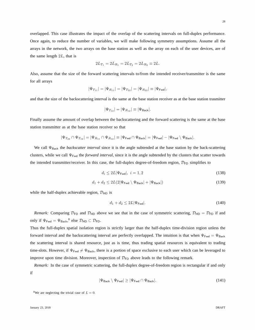
28

overlapped. This case illustrates the impact of the overlapof the scattering intervals on full-duplex performance.

Once again, to reduce the number of variables, we will make following symmetry assumptions. Assume all the

arrays in the network, the two arrays on the base station as well as the array on each of the user devices, are of

the same length2L, that is

2LT1= 2LR1

= 2LT2= 2LR2

≡ 2L.

Also, assume that the size of the forward scattering intervals to/from the intended receiver/transmitter is the same

for all arrays

|ΨT11| = |ΨR11

| = |ΨT22| = |ΨR22

| ≡ |ΨFwd|,

and that the size of the backscattering interval is the same at the base station receiver as at the base station trasmitter

|ΨT12| = |ΨR12

| ≡ |ΨBack|.

Finally assume the amount of overlap between the backscattering and the forward scattering is the same at the base

station transmitter as at the base station receiver so that

|ΨT22∩ΨT12

| = |ΨR11∩ΨR12

| ≡ |ΨFwd ∩ΨBack| = |ΨFwd| − |ΨFwd \ΨBack|.

We callΨBack the backscatter intervalsince it is the angle subtended at the base station by the back-scattering

clusters, while we callΨFwd the forward interval, since it is the angle subtended by the clusters that scattertowards

the intended transmitter/receiver. In this case, the full-duplex degree-of-freedom region,DFD simplifies to

di ≤ 2L|ΨFwd|, i = 1, 2 (138)

d1 + d2 ≤ 2L(2|ΨFwd \ΨBack|+ |ΨBack|) (139)

while the half-duplex achievable region,DHD is

d1 + d2 ≤ 2L|ΨFwd|. (140)

Remark: ComparingDFD andDHD above we see that in the case of symmetric scattering,DHD = DFD if and

only if ΨFwd = ΨBack,8 elseDHD ⊂ DFD.

Thus the full-duplex spatial isolation region is strictly larger than the half-duplex time-division region unless the

forward interval and the backscattering interval are perfectly overlapped. The intuition is that whenΨFwd = ΨBack

the scattering interval is shared resource, just as is time,thus trading spatial resources is equivalent to trading

time-slots. However, ifΨFwd 6= ΨBack, there is a portion of space exclusive to each user which can be leveraged to

improve upon time division. Moreover, inspection ofDFD above leads to the following remark.

Remark: In the case of symmetric scattering, the full-duplex degree-of-freedom region is rectangular if and only

if

|ΨBack \ΨFwd| ≥ |ΨFwd ∩ΨBack|. (141)

8We are neglecting the trivial case ofL = 0.

January 23, 2018 DRAFT

29

The above remark can be verified by comparing (138) and (139) observing that the sum-rate bound, (139), is only

active when

2|ΨFwd \ΨBack|+ |ΨBack| ≥ 2|ΨFwd|. (142)

Straightforward set-algebraic manipulation of condition(142) shows that it is equivalent to (141). The intuition is

that becauseΨBack \ ΨFwd are the set directions in which the base station couples to itself but not to the users,

the corresponding2L|ΨBack \ΨFwd| dimensions are useless for spatial multiplexing, and therefore “free” for zero

forcing the self-interference, which has maximum dimension 2L|ΨFwd ∩ ΨBack|. Thus when|ΨBack \ ΨFwd| ≥

|ΨFwd ∩ ΨBack|, we can zero force any self-interference that is generated,without sacrificing any resource needed

for spatial multiplexing to intended users.

Consider a numerical example in which|ΨFwd| = 1 and |ΨBack| = 1, thus the overlap between the two,|ΨFwd ∩

ΨBack|, can vary from zero to one. Figure 5 plots the half-duplex region, DHD, and the full-duplex region,DFD, for

several different values of overlap,|ΨFwd ∩ ΨBack|. We see that whenΨFwd = ΨBack so that|ΨFwd ∩ ΨBack| = 1,

bothDHD andDFD are the same triangular region. When|ΨFwd∩ΨBack| = 0.75, we get a rectangular region. Once

|ΨFwd ∩ ΨBack| ≤ 0.5, |ΨBack \ ΨFwd| becomes greater than 0.5, such that condition of (141) is satisfied and the

degree-of-freedom region becomes rectangular.

L2

L 3L2

2L

L2

L

3L2

2L

d1

d2

DHD

DFD: |ΨFwd ∩ΨBack| = 1

DFD: |ΨFwd ∩ΨBack| = 0.75

DFD: |ΨFwd ∩ΨBack| ≤ 0.5

Fig. 5: Symmetric-spread degree-of-freedom regions for different amounts of scattering overlap

V. CONCLUSION

Full-duplex operation presents an opportunity for base stations to as much as double their spectral efficiency by

both transmitting downlink signal and receiving uplink signal at the same time in the same band. The challenge to

full-duplex operation is high-powered self-interferencethat is received both directly from the base station transmitter

and backscattered from nearby objects. The receiver can be spatially isolated from the transmitter by leveraging

January 23, 2018 DRAFT

30

multi-antenna beamforming to avoid self-interference, but such beamforming can also decrease the degrees-of-

freedom of the intended uplink and downlink channels. We have leveraged a spatial antenna-theory-based channel

model to analyze the spatial degrees-of-freedom availableto a full-duplex base station. The analysis has shown

the full-duplex operation can indeed outperform half-duplex operation when either (1) the base station arrays are

large enough for for the base station to zero-force the backscattered self-interference or (2) the backscattering

directions are not fully overlapped with the forward scattering directions, so that the base station can leverage the

non-overlapped intervals for for interference free signaling to/from the intended users.

APPENDIX

A. Definitions

The following definitions are standard in functional analysis, but are refreshed here for clarity.

Definition 1: Let X be a Hilbert space, theorthogonal complementof S ⊆ X , denotedS⊥, is the subset

S⊥ ≡ x ∈ X : 〈x, u〉 = 0 ∀ u ∈ S.

Definition 2: Let X andY be vector spaces (e.g., Hilbert spaces) and letC : X → Y be a linear operator. Let

S ⊆ Y be a subspace ofY.

(i) The nullspaceof C, denotedN(C), is the subspace

N(C) ≡ x ∈ X : Cx = 0.

(ii) The rangeof C, denotedR(C), is the subspace

R(C) ≡ Cx : x ∈ X.

(iii) The preimageof S underC, C←(S), is the subspace (one can check that ifS is a subspace thenC←(S) is a

subspace also).

C←(S) ≡ x ∈ X : Cx ∈ S.

(iv) The rank of C is the dimension of the range ofC. A fundamental result in functional analysis is that the

dimension of the range ofC is also the dimension of the orthogonal complement of the nullspace ofC (i.e.

the coimage ofC) so that we can write

rankC ≡ dimR(C) = dimN(C)⊥.

B. Functional Analysis Lemmas

The following lemmas are general lemmas on compact operators on Hilbert spaces that will prove useful. We

state without proof the following result from functional analysis (see Section 16.1 and 16.2 of [26] for proof).

Lemma 5:Let X andY be Hilbert spaces and letC : X → Y be a compact linear operator. There exists asingular

systemσk, vk, uk, for C defined as follows. The set of functionsuk form an orthonormal basis forR(C), the

closure of the range ofC, and the set of functionsvk form an orthonormal basis forN(C)⊥, the coimage ofC.

January 23, 2018 DRAFT

31

The set of positive real numbersσk, called thesingular valuesof C, are the nonzero eigenvalues of(C∗C) arranged

in decreasing order. The singular system diagonalizesC in the sense that for any(σk, vk, uk) ∈ σk, vk, uk,

Cvk = σkuk. (143)

Moreover, the operation ofC on anyx ∈ X can be expanded as

Cx =∑

k

σk〈x, vk〉uk, (144)

which is called the singular value expansion ofCx.

The next Lemma is a well-known characterization of the properties of the Moore-Penrose generalized inverse,

and the conditions sufficient for its existence.

Lemma 6:Let X andY be Hilbert spaces and letC : X → Y be a linear operator with closed range. There

exists a unique linear operatorC+, called theMoore-Penrose pseudoinverseof C, with the following properties:

(i) C+Cx = x ∀x ∈ N(C)⊥

(ii) CC+y = y ∀y ∈ R(C)

(iii) R(C+) = N(C)⊥

(iv) N(C+) = R(C)⊥.

Proof: See Definition 2.2 and Proposition 2.3 of [27].

Lemma 7:Let X andY be finite-dimensional Hilbert spaces and letC : X → Y be a linear operator with closed

range. LetS ⊆ Y be a subspace ofY. Then the dimension of the preimage ofS underC is

dimC←(S) = dimN(C) + dim(R(C) ∩ S). (145)

Proof: For notational convenience, letdP ≡ dimC←(S), dN ≡ dimN(C), anddR∩S ≡ dim(R(C)∩S). Thus

we wish to show thatdP = dN + dR∩S . First note thatN(C) ⊆ C←(S), sinceS is a subspace and hence contains

the zero vector, and the preimage of the zero vector underC is the nullspace ofC. Denote the intersection between

the preimage ofS underC and the orthogonal complement of the nullspace ofC (i.e. the coimage) as

B ≡ C←(S) ∩N(C)⊥. (146)

Note thatB is a subspace ofX since the intersection of any collection of subspaces is itself a subspace (see Thm.

1 on p. 3 of [32]). Everyx ∈ C←(S) can be expressed asx = w + u for somew ∈ N(C) and u ∈ B, and

〈w, u〉 = 0 for any w ∈ N(C) andu ∈ B. Thus we can say that the preimage,C←(S), is theorthogonal direct

sumof subspacesN(C) andB ([26] Def. 4.26), a relationship we note we denote as

C←(S) = N(C)⊕ B. (147)

Let aidN

i=1 be a basis forN(C) andbidB

i=1 be a basis forB, wheredN = dimN(C) anddB = dimB. Construct

the seteidN+dB

i=1 according to

eidN

i=1 = aidN

i=1, eidN+dB

i=dN+1 = bidB

i=1. (148)

January 23, 2018 DRAFT

32

We claim thateidN+dB

i=1 forms a basis forC←(S). To check thateidN+dB

i=1 is a basis forC←(S), we must first

showeidN+dB

i=1 spansC←(S), and then show that the elements ofeidN+dB

i=1 are linearly independent. Consider

an arbitraryx ∈ C←(S). SinceC←(S) = N(C) ⊕ B, x = w + u for somew ∈ N(C) and u ∈ B. Since by

constructioneidN

i=1 is a basis forN(C) and eidN+dB

i=1+dNis a basis forN(C), one can chooseλi such that that

w =∑dN

i=1 λiei andu =∑dN+dB

i=1+dNλiei. Thus

x = w + v =

dN∑

i=1

λiei +

dN+dB∑

i=1+dN

λiei =

dN+dB∑

i=1

λiei (149)

for someλi. ThuseidN+dB

i=1 spansC←(S). Now let us show linear independence: that∑dN+dB

i=1 λiei = 0 if and

only if λi = 0 for all i ∈ 1, 2, . . . , dN+dB. The “if” part is trivial, thus it remains to show that∑dN+dB

i=1 λiei = 0

implies λi = 0 ∀i. The condition∑dN+dB

i=1 λiei = 0 implies

dN∑

i=1

λiei = −

dN+dB∑

i=dN+1

λiei, (150)

which impliesw = −u for somew ∈ N(C) andu ∈ B. Every element ofN(C) is orthogonal to every element

of B by construction, hence the only way Equation (150) can be satisfied is if w = u = 0, that is if both sides

of Equation (150) are zero, implyingλi = 0 for all i ∈ 1, 2, . . . , dN + dB as desired. Thus we have shown

eidN+dB

i=1 is a basis forC←(S), and hence

dP = dN + dB. (151)

Consider the setCeidN+dB

i=1+dN. By the definition of range, each element of the setCei

dN+dB

i=1+dNis in R(C), and

since by construction eachei is in C←(S), each element ofCeidN+dB

i=1+dNis also inS. We therefore have that

spanCeidN+dB

i=1+dN⊆ R(C) ∩ S, (152)

and since there aredB elements inCeidN+dB

i=1+dN, it must be that

dB ≤ dR∩S . (153)

Substituting the above inequality into Equation (151) gives

dP ≤ dN + dR∩S . (154)

To complete the proof we must show thatdP ≥ dN + dR∩S . Let sidR∩S

i=1 be a basis forR(C) ∩ S. By

assumptionR(C) is closed, thus we have by Lemma 6 that the Moore-Penrose pseudoinverse,C+, exists, and

satisfies the properties listed in Lemma 6. Consider the setC+sidR∩S

i=1 . We claim that

spanC+sidR∩S

i=1 ⊆ N(C)⊥ ∩ C←(S) ≡ B. (155)

By property (iv) in Lemma 6, we have thatC+si ∈ N(C)⊥ for eachC+si ∈ C+sidR∩S

i=1 . Sincesi ∈ R(C), we

have thatC(C+si) = si by property (ii) of the pseudoinverse, and sincesi ∈ S, we have thatCC+si = si ∈ S for

eachC+si ∈ C+sidR∩S

i=1 . Thus each element ofC+sidR∩S

i=1 is also inC←(S), the preimage ofS underC. Thus

January 23, 2018 DRAFT

33

we have that each element ofC+sidR∩S

i=1 is in N(C)⊥ ∩C←(S) which justifies the claim of Equation (155). Now

equation Equation (155) implies that

dR∩S ≤ dB (156)

Substituting the above inequality into Equation (151) gives

dP ≥ dN + dR∩S , (157)

concluding the proof.

Corollary 1: Let X andY be finite-dimensional Hilbert spaces and letC : X → Y be a linear operator with

closed range. LetS ⊆ R(C) ⊆ Y be a subspace of the range ofC. Then the dimension of the preimage ofS under

C is

dimC←(S) = dimN(C) + dim(S). (158)

Proof: The proof follows trivially from Lemma 7 by noting that sinceS ⊆ R(C), R(C) ∩ S = S, which we

substitute into equation 145 to obtain the corollary.

REFERENCES

[1] D. W. Bliss, P. A. Parker, and A. R. Margetts, “Simultaneous transmission and reception for improved wireless network performance,” in

Proceedings of the 2007 IEEE/SP 14th Workshop on Statistical Signal Processing, 2007, pp. 478–482.

[2] A. K. Khandani, “Methods for spatial multiplexing of wireless two-way channels,” US Patent US 7 817 641, October 19, 2010.

[3] B. Radunovic, D. Gunawardena, P. Key, A. P. N. Singh, V. Balan, and G. Dejean, “Rethinking indoor wireless: Low power,low frequency,

full duplex,” Microsoft Technical Report, Tech. Rep., 2009.

[4] M. Duarte and A. Sabharwal, “Full-duplex wireless communications using off-the-shelf radios: Feasibility and first results,” inProc. 2010

Asilomar Conference on Signals and Systems, 2010.

[5] J. I. Choi, M. Jain, K. Srinivasan, P. Levis, and S. Katti,“Achieving single channel, full duplex wireless communication,” in MobiCom

2010.

[6] M. Jain, J. I. Choi, T. Kim, D. Bharadia, S. Seth, K. Srinivasan, P. Levis, S. Katti, and P. Sinha, “Practical, real-time, full duplex

wireless,” in Proceedings of the 17th annual international conference onMobile computing and networking, ser. MobiCom ’11. New

York, NY, USA: ACM, 2011, pp. 301–312. [Online]. Available:http://doi.acm.org/10.1145/2030613.2030647

[7] M. Duarte, C. Dick, and A. Sabharwal, “Experiment-driven characterization of full-duplex wireless systems,”Wireless Communications,

IEEE Transactions on, vol. 11, no. 12, pp. 4296–4307, 2012.

[8] A. Sahai, G. Patel, and A. Sabharwal, “Pushing the limitsof full-duplex: Design and real-time implementation,” Rice Univeristy, Tech.

Rep. TREE1104, 2011.

[9] M. A. Khojastepour, K. Sundaresan, S. Rangarajan, X. Zhang, and S. Barghi, “The case for antenna cancellation for scalable full-duplex

wireless communications,” inProceedings of the 10th ACM Workshop on Hot Topics in Networks, ser. HotNets-X. New York, NY,

USA: ACM, 2011, pp. 17:1–17:6. [Online]. Available: http://doi.acm.org/10.1145/2070562.2070579

[10] E. Aryafar, M. A. Khojastepour, K. Sundaresan, S. Rangarajan, and M. Chiang, “Midu: enabling mimo full duplex,” inProceedings of

the 18th annual international conference on Mobile computing and networking, ser. Mobicom ’12. New York, NY, USA: ACM, 2012,

pp. 257–268. [Online]. Available: http://doi.acm.org/10.1145/2348543.2348576

[11] M. Duarte, A. Sabharwal, V. Aggarwal, R. Jana, K. Ramakrishnan, C. Rice, and N. Shankaranarayanan, “Design and characterization of

a full-duplex multiantenna system for wifi networks,”Vehicular Tech., IEEE Trans. on, vol. 63, no. 3, pp. 1160–1177, 2014.

[12] M. Duarte, “Full-duplex wireless: Design, implementation and characterization,” Ph.D. dissertation, Rice University, April 2012. [Online].

Available: http://warp.rice.edu/trac/wiki/DuartePhDThesis

January 23, 2018 DRAFT

34

[13] B. Day, A. Margetts, D. Bliss, and P. Schniter, “Full-duplex bidirectional MIMO: Achievable rates under limited dynamic range,”Signal

Processing, IEEE Trans. on, vol. 60, no. 7, pp. 3702 –3713, jul. 2012.

[14] ——, “Full-duplex MIMO relaying: Achievable rates under limited dynamic range,”Selected Areas in Communications, IEEE Journal on,

vol. 30, no. 8, pp. 1541 –1553, september 2012.

[15] E. Everett, M. Duarte, C. Dick, and A. Sabharwal, “Empowering full-duplex wireless communication by exploiting directional diversity,”

in Asilomar Conference on Signals, Systems and Computers, October 2011.

[16] E. Everett, A. Sahai, and A. Sabharwal, “Passive self-interference suppression for full-duplex infrastructure nodes,”Wireless Comm., IEEE

Trans. on, vol. 13, no. 2, pp. 680–694, Feb. 2014.

[17] A. Sahai, G. Patel, C. Dick, and A. Sabharwal, “On the impact of phase noise on active cancelation in wireless full-duplex,” Vehicular

Technology, IEEE Transactions on, vol. 62, no. 9, pp. 4494–4510, 2013.

[18] A. Sabharwal, P. Schniter, D. Guo, D. W. Bliss, S. Rangarajan, and R. Wichman, “In-band full-duplex wireless: Challenges and

opportunities,”CoRR, vol. abs/1311.0456, 2013.

[19] A. Poon, R. Brodersen, and D. Tse, “Degrees of freedom inmultiple-antenna channels: a signal space approach,”Information Theory,

IEEE Transactions on, vol. 51, no. 2, pp. 523 – 536, feb. 2005.

[20] A. Poon, D. Tse, and R. Brodersen, “Impact of scatteringon the capacity, diversity, and propagation range of multiple-antenna channels,”

Information Theory, IEEE Transactions on, vol. 52, no. 3, pp. 1087 –1100, march 2006.

[21] A. Poon and D. Tse, “Degree-of-freedom gain from using polarimetric antenna elements,”Information Theory, IEEE Transactions on,

vol. 57, no. 9, pp. 5695 –5709, sept. 2011.

[22] A. Poon and M. Ho, “Indoor multiple-antenna channel characterization from 2 to 8 ghz,” inCommunications, 2003. ICC ’03. IEEE

International Conference on, vol. 5, 2003, pp. 3519–3523 vol.5.

[23] Q. Spencer, B. Jeffs, M. Jensen, and A. Swindlehurst, “Modeling the statistical time and angle of arrival characteristics of an indoor

multipath channel,”Selected Areas in Communications, IEEE Journal on, vol. 18, no. 3, pp. 347–360, 2000.

[24] R. J.-M. Cramer, “An evaluation of ultra-wideband propagation channels,” Ph.D. dissertation, University of Southern California, 2000.

[25] R. Heddergott and P. Truffer, “Statistical characteristics of indoor radio propagation in nlos scenarios,” EUROPEAN COOPERATION IN

THE FIELD OF SCIENTIFIC AND TECHNICAL RESEARCH, Valencia, Spain, Tech. Rep. COST 259 TD(00) 024, 2000.

[26] N. Young,An Introduction to Hilbert Space. Cambridge University Press, 1988.

[27] H. W. Engl, M. Hanke, and A. Neubauer,Regularization of Inverse Problems. Kluwer Academic Publishers, 1996.

[28] E. Telatar, “Capacity of multi-antenna gaussian channels,” European Transactions on Telecommunications, vol. 10, no. 6, pp. 585–595,

1999.

[29] L. Ke and Z. Wang, “Degrees of freedom regions of two-user mimo z and full interference channels: The benefit of reconfigurable

antennas,”Information Theory, IEEE Transactions on, vol. 58, no. 6, pp. 3766–3779, 2012.

[30] S. Jafar and M. Fakhereddin, “Degrees of freedom for themimo interference channel,”Information Theory, IEEE Transactions on, vol. 53,

no. 7, pp. 2637–2642, 2007.

[31] S. Krishnamurthy and S. Jafar, “Degrees of freedom of 2-user and 3-user rank-deficient mimo interference channels,” in Global

Communications Conference (GLOBECOM), 2012 IEEE, Dec 2012, pp. 2462–2467.

[32] P. D. Lax,Funtional Analysis. John Wiley and Sons Inc., 2002.

January 23, 2018 DRAFT