Sparsity in Linear Least SquaresGraph Theoretic Approaches to Sparse

Factorization

Manmohan Krishna Chandraker

CSE 252C, Fall 2004, UCSD

– p.1

Linear Least Squares Problem

• Find x ∈ Rn that minimizes

minx

‖Ax − b‖, A ∈ Rm×n, b ∈ R

m, m ≥ n.

• Residual vector, r = b −Ax.

• Sparse LLS : A is sparse.

Sparse Linear Least Squares – p.2

Is Sparsity Useful?

• Electric grids• Geodetic measurements• Bundle adjustment

Sparse Linear Least Squares – p.3

Characterization of LS solutions

• Normal Equations• x is a solution to the Least Squares problem if and

only if

A⊤Ax = A⊤b

• Solution method : Cholesky Decomposition

• QR decomposition• min

x

‖Ax− b‖ = minx

‖Q⊤(Ax− b)‖ for Q ∈ SO(m).

Sparse Linear Least Squares – p.4

Time Complexity of DirectMethods

• Structure of A influences choice of algorithm.

Ax = b

• Dense - Gaussian elimination :2

3n3 + O(n2) flops.

• Symmetric, positive definite - Cholesky

decomposition :1

3n3 + O(n2) flops.

• Triangular - Simple substitution : n2 + O(n).

Sparse Linear Least Squares – p.5

What kind of sparsity is useful?

• When there are O(n) non-zero entries.• Sparse data structures include more storage

overhead.

• Arithmetic operations are slower (due to indirectaddressing).

• When the sparsity has a pattern.

Sparse Linear Least Squares – p.6

Sparse Data StructuresStatic, compressed row storage

A =

a11 0 a13 0 0

a21 a22 0 0 0

0 0 a33 0 0

0 a42 0 a44 0

0 0 0 a54 a55

0 0 0 0 a65

AC = (a11 , a13 | a22 , a21 | a33 | a42 , a44 | a54 , a55 | a65)

IA = (1, 3, 5, 6, 8, 10, 11)

JA = (1, 3, 2, 1, 3, 2, 4, 4, 5, 5)

Sparse Linear Least Squares – p.7

Gaussian Elimination: Fill-in

Fill-in : Non-zero elements created by Gaussianelimination.

A = A(1) =

[

a r⊤

c A

]

where a ∈ R1×1, A ∈ R

(n−1)×(n−1)

A(1) =

[

1 0c

aI

] [

a r⊤

0 A(2)

]

⇒ A(2) = A −

(

cr⊤

a

)

Repeat same for A(2), say, A(2) = L2U2.

Sparse Linear Least Squares – p.8

Processing Order and Fill-in

• Column order greatly affects fill-in.

× × ×

× × ×

× ×

× × ×

× ×

× × ×

× × ×

× ×

× × ×

× ×

• Find the column order that minimizes fill-in :

Sparse Linear Least Squares – p.9

Processing Order and Fill-in

• Column order greatly affects fill-in.

× × ×

× × ×

× ×

× × ×

× ×

× × ×

× × ×

× ×

× × ×

× ×

• Find the column order that minimizes fill-in :NP-complete!!

Sparse Linear Least Squares – p.10

Steps in a Sparse LS Problem

Symbolic factorization

• Find the structure of A⊤A.

• Determine a column order that reduces fill-in.

• Predict the sparsity structure of the decomposition andallocate storage.

Numerical solution

• Read numerical values into the data structure.

• Do a numerical factorization and solve.

Sparse Linear Least Squares – p.11

Graph for Sparse SymmetricMatrix

× × × ×

× × ×

× × × ×

× ×

× ×

× ×

× ×

• A node vi for each column i

• (vi, vj) ∈ E ⇔ aij 6= 0

Symbolic Factorization – p.12

Predicting Structure ofA⊤A

• A⊤A =m

∑

i=1

aia⊤i where a⊤

i = i-th row of A.

• G(A⊤A) = direct sum of G(a⊤i ai),

i = 1, · · · ,m.

• Non-zeros in a⊤i form a clique subgraph.

Symbolic Factorization – p.13

Predicting Structure of CholeskyFactorR

Elimination Graphs : Represent fill-in duringfactorization.

Symbolic Factorization – p.14

Filled Graph• GF (A) : Direct sum of elimination graphs.

Symbolic Factorization – p.15

Structure of Cholesky Factor• Filled graph bounds structure of Cholesky factor

G(R + R⊤) ⊂ GF (A)

• Equality when no-cancellation holds.A R

× × × ×

× × ×

× × × ×

× ×

× ×

× ×

× ×

× × × ×

× × × ×

× × × × ×

× × × ×

× × ×

× ×

×

Symbolic Factorization – p.16

Efficient Computation of FilledGraph

• Theorem : Let G(A) = (V,E) be an orderedgraph of A. Then (vi, vj) is an edge of thefilled graph GF (A) if and only if (vi, vj) ∈ E orthere is a path in G(A) from vertex vi to vj

passing only through vertices with numberingless than min{i, j}.

• Allows construction of filled graph in O(n|E|)time.

Symbolic Factorization – p.17

Fill Minimizing ColumnOrderings

• Reordering rows of A does not affect A⊤A.• Column reordering in A keeps number of

non-zeros same in A⊤A.• Greatly affects number of non-zeros in R.• Heuristics to reduce fill-in :

• Minimum degree ordering

• Nested dissection orderings.

Symbolic Factorization – p.18

Minimum Degree Ordering

Let G(0) = G(A).

for i = 1, · · · , (n − 1) :

Select a node v in G(i−1) of minimal degree.Choose v as next pivot.

Update elimination graph to get G(i).

end

Symbolic Factorization – p.19

Without Ordering

Order 1, 2, 3, 4, 5, 6, 7 → fill-in = 10.

Symbolic Factorization – p.20

With Minimum Degree Ordering

Order 4, 5, 6, 7, 1, 2, 3 → fill-in = 0 !!

Symbolic Factorization – p.21

Does not always work!

• Order 1, 2, · · · , 9 → fill-in = 0.• Minimum degree node : 5 → fills in (4, 6).

Symbolic Factorization – p.22

Nested Dissection Ordering

• Reorder to obtain block angular sparsematrix.

1 23 4

Symbolic Factorization – p.23

Nested Dissection: BlockStructure and Elimination Tree

A =

2

4

A1 B1

A2 B2

3

5 A =

2

6

6

6

6

6

4

A1 B1 D1

A2 B2 D2

A3 C3 D3

A4 C4 D4

3

7

7

7

7

7

5

1 2 3 4

Symbolic Factorization – p.24

Numerical Factorization

• Mathematically, Cholesky factor of A⊤A

same as R in QR-decomposition of A.

• Numerical issues govern choice of algorithm.

• Symbolic factorization same for both.

Numerical Factorization – p.25

Numerical Cholesky FactorizationSymbolic Phase

1. Find symbolic structure of A⊤A.

2. Find column permutation Pc such that P⊤c A⊤APc has

sparse Cholesky factor R.

3. Perform symbolic factorization and generate storagestructure for R.

Numerical Phase

1. Compute B = P⊤c A⊤APc and c = P⊤

c A⊤b numerically.

2. Compute R numerically and solve R⊤z = c, Ry = z,x = Pcy.

Numerical Factorization – p.26

Cholesky vs QR

• Symbolic computation: No pivoting forneeded for Cholesky.

• Loss of information in A⊤A and A⊤b.• Condition number squared in A⊤A.• Inefficient memory utilization: both rows and

columns accessed in elimination.

Numerical Factorization – p.27

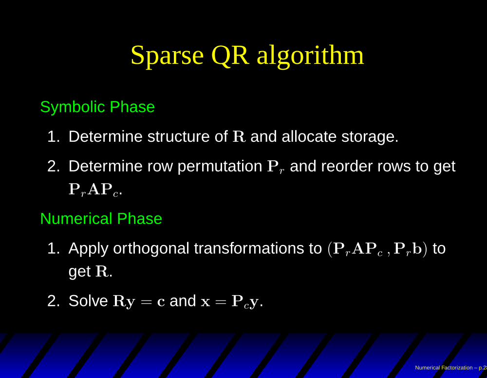
Sparse QR algorithm

Symbolic Phase

1. Determine structure of R and allocate storage.

2. Determine row permutation Pr and reorder rows to getPrAPc.

Numerical Phase

1. Apply orthogonal transformations to (PrAPc ,Prb) toget R.

2. Solve Ry = c and x = Pcy.

Numerical Factorization – p.28

QR-Decomposition

• Dense problems: Sequence of Householderreflections.

• Sparse problems: Intermediate fill-in.• Expensive computation and storage.• Row sequential QR-decomposition.

Numerical Factorization – p.29

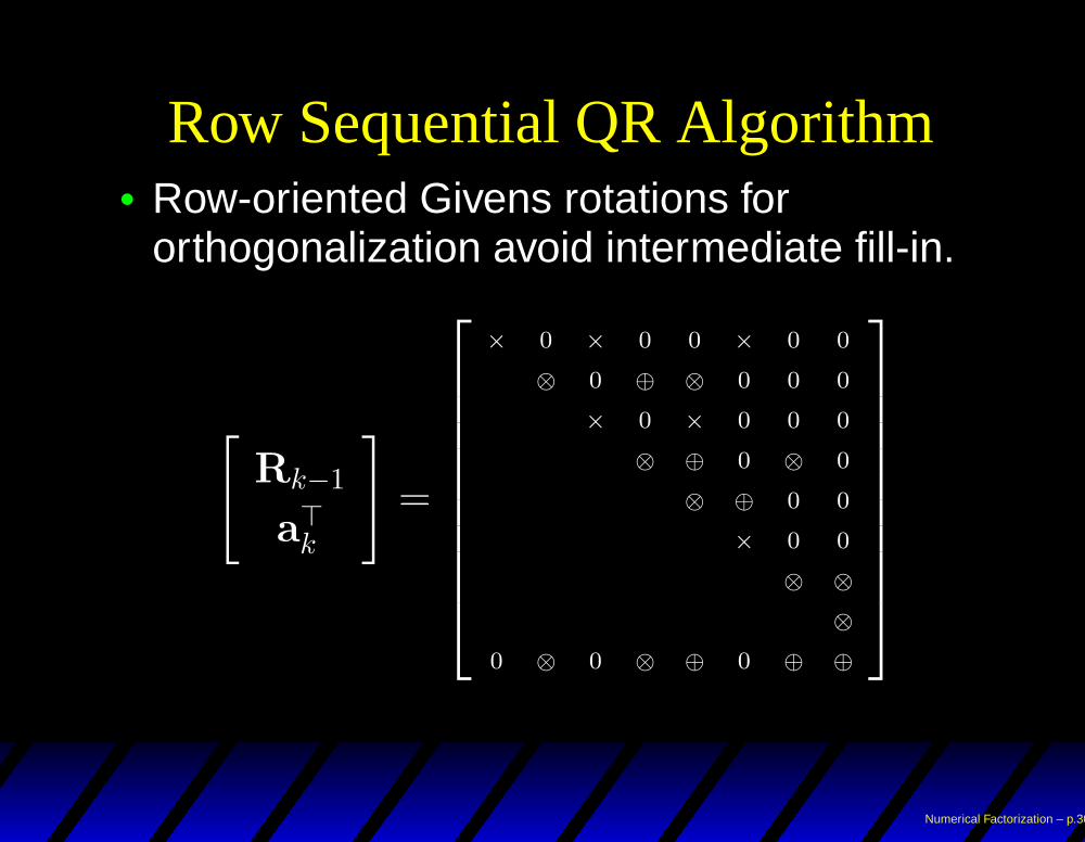
Row Sequential QR Algorithm• Row-oriented Givens rotations for

orthogonalization avoid intermediate fill-in.

[

Rk−1

a⊤k

]

=

× 0 × 0 0 × 0 0

⊗ 0 ⊕ ⊗ 0 0 0

× 0 × 0 0 0

⊗ ⊕ 0 ⊗ 0

⊗ ⊕ 0 0

× 0 0

⊗ ⊗

⊗

0 ⊗ 0 ⊗ ⊕ 0 ⊕ ⊕

Numerical Factorization – p.30

Summary• Exploiting sparsity: storage and time savings.• A sparse LS problem can be subdivided into

a symbolic phase and a numerical phase.• The symbolic phase:

• Determines a column ordering that makes theCholesky factor sparse.

• Determines the structure of the Cholesky factor.

• The numerical phase:• Uses specialized orthogonalization algorithms to

determine the numerical factorization.

Numerical Factorization – p.31