Sparsely Precomputing The Light Transport Matrix for

Real-Time Rendering

Fu-Chung HuangRavi Ramamoorthi

Electrical Engineering and Computer SciencesUniversity of California at Berkeley

Technical Report No. UCB/EECS-2010-79

http://www.eecs.berkeley.edu/Pubs/TechRpts/2010/EECS-2010-79.html

May 14, 2010

Copyright © 2010, by the author(s).All rights reserved.

Permission to make digital or hard copies of all or part of this work forpersonal or classroom use is granted without fee provided that copies arenot made or distributed for profit or commercial advantage and that copiesbear this notice and the full citation on the first page. To copy otherwise, torepublish, to post on servers or to redistribute to lists, requires prior specificpermission.

Acknowledgement

This work was supported in part by NSF CAREER grant IIS-0924968 andONR PECASE grant N00014-09-1-0741, as well as equipment andgenerous support from Intel, NVIDIA, Adobe, and Pixar.

Sparsely Precomputing The Light Transport Matrix forReal-Time Rendering

Fu-Chung Huang and Ravi Ramamoorthi

University of California at Berkeley, USA

Abstract

Precomputation-based methods have enabled real-time rendering with natural illumination, all-frequency shad-ows, and global illumination. However, a major bottleneck is the precomputation time, that can take hours todays. While the final real-time data structures are typically heavily compressed with clustered principal compo-nent analysis and/or wavelets, a full light transport matrix still needs to be precomputed for a synthetic scene, oftenby exhaustive sampling and raytracing. This is expensive and makes rapid prototyping of new scenes prohibitive.In this paper, we show that the precomputation can be made much more efficient by adaptive and sparse samplingof light transport. We first select a small subset of “dense vertices”, where we sample the angular dimensions morecompletely (but still adaptively). The remaining “sparse vertices” require only a few angular samples, isolatingfeatures of the light transport. They can then be interpolated from nearby dense vertices using locally low rankapproximations. We demonstrate sparse sampling and precomputation5× faster than previous methods.

1. Introduction

Precomputation-based rendering, or precomputed radiancetransfer (PRT), has enabled real-time image synthesis withnatural lighting, intricate shadows, and global illuminationeffects [SKS02, NRH03]. However, the initial precomputa-tion remains a bottleneck, since the full light transport matrixneeds to first be precomputed, corresponding to each vertexand light source direction. To include interreflection effects,exhaustive sampling and ray or path tracing is typically re-quired. For an all-frequency lighting cubemap resolution of6× 32× 32, the cost is essentially equivalent to rendering6144 images, and can take hours to days. This precludesrapidly prototyping new scenes, and hinders adoption.

The final data structure for real-time rendering is highlycompressed, such as with wavelets or clustered principalcomponent analysis (CPCA) [SHHS03,LSSS04], but thesemethods first require the full light transport to be available.This paper investigates fast precomputation by adaptive andsparse sampling of light transport. While our technique issimple and broadly applicable to almost any PRT system,we focus on all-frequency relighting of static geometry, in-cluding interreflection effects, where the precomputationisby explicit sampling and ray tracing. This includes both thediffuse geometry relighting of Ng et al. [NRH03], and itsextension to glossy materials with BRDF in-out factoriza-

tion [LSSS04, WTL04]—in the latter case, our method issimply applied to each view-independent transport term.

We leverage key recent insights about the structure oflight transport. CPCA [SHHS03] is based on assumingthat locally, the response of vertices is similar, and of lowrank [MKSRB07]. Hence, we first compute a small sub-set of “dense” vertices, where almost all angular direc-tions are sampled. The remaining “sparse” vertices requireonly a few light source directions to be computed, andcan then be reconstructed with a low rank approximationfrom their neighbors. We also know that light transport issparse [NRH03,PML∗09]. We exploit this idea by focusingour sampling on those angular directions that correspond tofeatures, and by using recent sparseL1 minimization meth-ods [KKL ∗07]. Our algorithm includes simple heuristics tochoose the best candidate “dense” spatial vertices and angu-lar features.

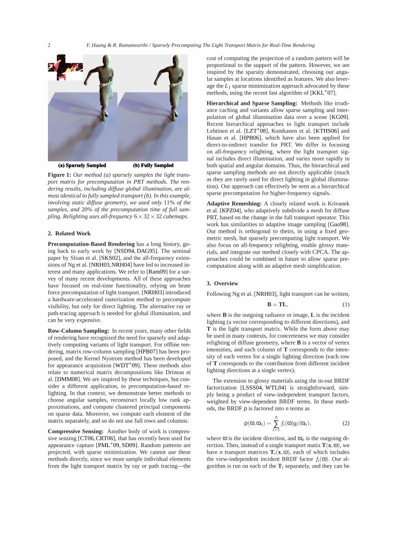
As shown in Fig.1, we can produce accurate results withexplicit precomputation of only about 11% of the light trans-port matrix, and with acceptable overheads (wall clock timeis 20% of brute force precomputation). These results poten-tially enable new capabilities for rapid prototyping of scenes,or shots for lighting design.

2 F. Huang & R. Ramamoorthi / Sparsely Precomputing The Light Transport Matrix for Real-Time Rendering

Figure 1: Our method (a) sparsely samples the light trans-port matrix for precomputation in PRT methods. The ren-dering results, including diffuse global illumination, are al-most identical to fully sampled transport (b). In this example,involving static diffuse geometry, we used only11% of thesamples, and20% of the precomputation time of full sam-pling. Relighting uses all-frequency6×32×32cubemaps.

2. Related Work

Precomputation-Based Renderinghas a long history, go-ing back to early work by [NSD94, DAG95]. The seminalpaper by Sloan et al. [SKS02], and the all-frequency exten-sions of Ng et al. [NRH03,NRH04] have led to increased in-terest and many applications. We refer to [Ram09] for a sur-vey of many recent developments. All of these approacheshave focused on real-time functionality, relying on bruteforce precomputation of light transport. [NRH03] introduceda hardware-accelerated rasterization method to precomputevisibility, but only for direct lighting. The alternative ray orpath-tracing approach is needed for global illumination, andcan be very expensive.

Row-Column Sampling: In recent years, many other fieldsof rendering have recognized the need for sparsely and adap-tively computing variants of light transport. For offline ren-dering, matrix row-column sampling [HPB07] has been pro-posed, and the Kernel Nystrom method has been developedfor appearance acquisition [WDT∗09]. These methods alsorelate to numerical matrix decompositions like Drineas etal. [DMM08]. We are inspired by these techniques, but con-sider a different application, to precomputation-based re-lighting. In that context, we demonstrate better methods tochoose angular samples, reconstruct locally low rank ap-proximations, and compute clustered principal componentson sparse data. Moreover, we compute each element of thematrix separately, and so do not use full rows and columns.

Compressive Sensing:Another body of work is compres-sive sensing [CT06,CRT06], that has recently been used forappearance capture [PML∗09, SD09]. Random patterns areprojected, with sparse minimization. We cannot use thesemethods directly, since we must sample individual elementsfrom the light transport matrix by ray or path tracing—the

cost of computing the projection of a random pattern will beproportional to the support of the pattern. However, we areinspired by the sparsity demonstrated, choosing our angu-lar samples at locations identified as features. We also lever-age theL1 sparse minimization approach advocated by thesemethods, using the recent fast algorithm of [KKL ∗07].

Hierarchical and Sparse Sampling: Methods like irradi-ance caching and variants allow sparse sampling and inter-polation of global illumination data over a scene [KG09].Recent hierarchical approaches to light transport includeLehtinen et al. [LZT∗08], Kontkanen et al. [KTHS06] andHasan et al. [HPB06], which have also been applied fordirect-to-indirect transfer for PRT. We differ in focusingon all-frequency relighting, where the light transport sig-nal includes direct illumination, and varies more rapidly inboth spatial and angular domains. Thus, the hierarchical andsparse sampling methods are not directly applicable (muchas they are rarely used for direct lighting in global illumina-tion). Our approach can effectively be seen as a hierarchicalsparse precomputation for higher-frequency signals.

Adaptive Remeshing:A closely related work is Krivaneket al. [KPZ04], who adaptively subdivide a mesh for diffusePRT, based on the change in the full transport operator. Thiswork has similarities to adaptive image sampling [Guo98].Our method is orthogonal to theirs, in using a fixed geo-metric mesh, but sparsely precomputing light transport. Wealso focus on all-frequency relighting, enable glossy mate-rials, and integrate our method closely with CPCA. The ap-proaches could be combined in future to allow sparse pre-computation along with an adaptive mesh simplification.

3. Overview

Following Ng et al. [NRH03], light transport can be written,

B = TL , (1)

whereB is the outgoing radiance or image,L is the incidentlighting (a vector corresponding to different directions), andT is the light transport matrix. While the form above maybe used in many contexts, for concreteness we may considerrelighting of diffuse geometry, whereB is a vector of vertexintensities, and each column ofT corresponds to the inten-sity of each vertex for a single lighting direction (each rowof T corresponds to the contribution from different incidentlighting directions at a single vertex).

The extension to glossy materials using the in-out BRDFfactorization [LSSS04, WTL04] is straightforward, sim-ply being a product of view-independent transport factors,weighted by view-dependent BRDF terms. In these meth-ods, the BRDFρ is factored inton terms as

ρ(ω,ωo) =n

∑i=1

fi(ω)gi(ωo), (2)

whereω is the incident direction, andωo is the outgoing di-rection. Then, instead of a single transport matixT(x,ω), wehaven transport matricesT i(x,ω), each of which includesthe view-independent incident BRDF factorfi(ω). Our al-gorithm is run on each of theT i separately, and they can be

F. Huang & R. Ramamoorthi / Sparsely Precomputing The Light Transport Matrix for Real-Time Rendering 3

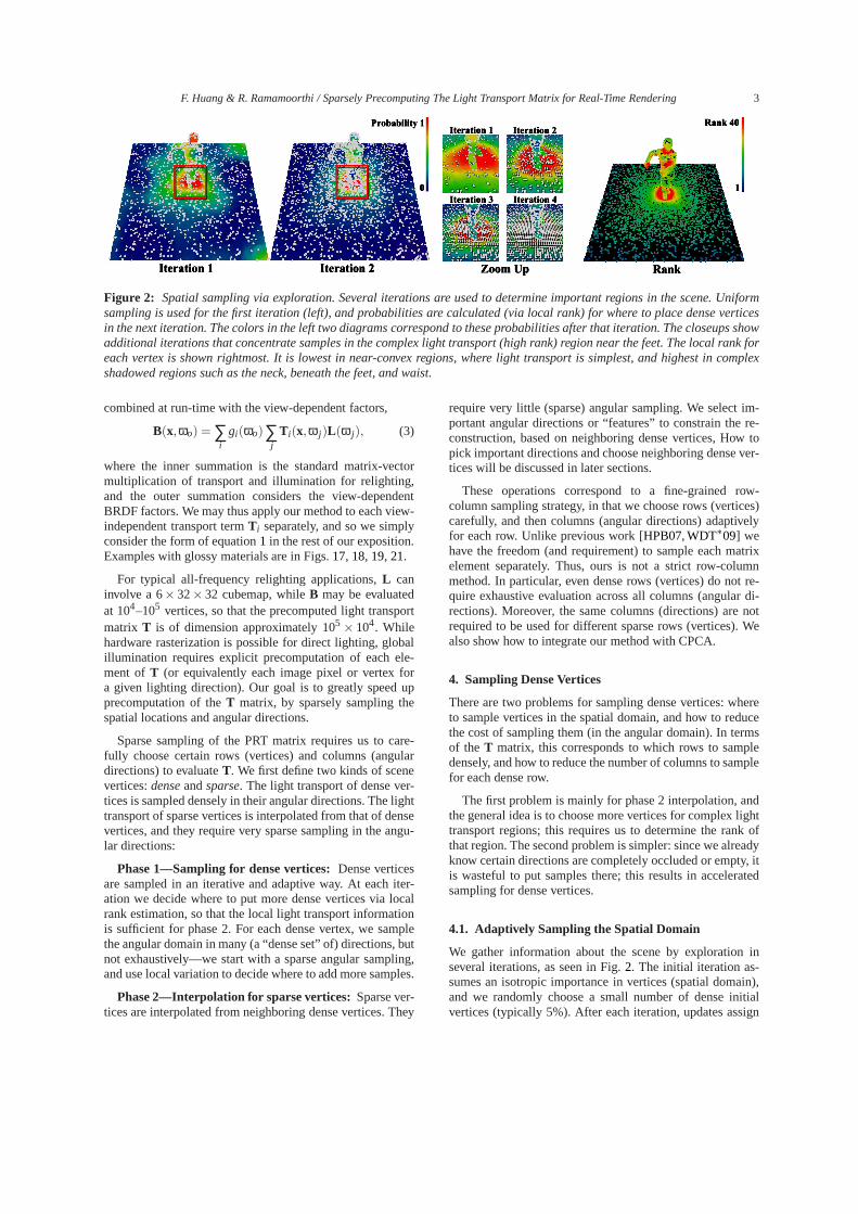
Figure 2: Spatial sampling via exploration. Several iterations are used to determine important regions in the scene. Uniformsampling is used for the first iteration (left), and probabilities are calculated (via local rank) for where to place dense verticesin the next iteration. The colors in the left two diagrams correspond to these probabilities after that iteration. The closeups showadditional iterations that concentrate samples in the complex light transport (high rank) region near the feet. The local rank foreach vertex is shown rightmost. It is lowest in near-convex regions, where light transport is simplest, and highest in complexshadowed regions such as the neck, beneath the feet, and waist.

combined at run-time with the view-dependent factors,

B(x,ωo) = ∑i

gi(ωo)∑j

T i(x,ω j )L(ω j), (3)

where the inner summation is the standard matrix-vectormultiplication of transport and illumination for relighting,and the outer summation considers the view-dependentBRDF factors. We may thus apply our method to each view-independent transport termT i separately, and so we simplyconsider the form of equation1 in the rest of our exposition.Examples with glossy materials are in Figs.17, 18, 19, 21.

For typical all-frequency relighting applications,L caninvolve a 6× 32×32 cubemap, whileB may be evaluatedat 104–105 vertices, so that the precomputed light transportmatrix T is of dimension approximately 105

× 104. Whilehardware rasterization is possible for direct lighting, globalillumination requires explicit precomputation of each ele-ment of T (or equivalently each image pixel or vertex fora given lighting direction). Our goal is to greatly speed upprecomputation of theT matrix, by sparsely sampling thespatial locations and angular directions.

Sparse sampling of the PRT matrix requires us to care-fully choose certain rows (vertices) and columns (angulardirections) to evaluateT. We first define two kinds of scenevertices:denseandsparse. The light transport of dense ver-tices is sampled densely in their angular directions. The lighttransport of sparse vertices is interpolated from that of densevertices, and they require very sparse sampling in the angu-lar directions:

Phase 1—Sampling for dense vertices:Dense verticesare sampled in an iterative and adaptive way. At each iter-ation we decide where to put more dense vertices via localrank estimation, so that the local light transport informationis sufficient for phase 2. For each dense vertex, we samplethe angular domain in many (a “dense set” of) directions, butnot exhaustively—we start with a sparse angular sampling,and use local variation to decide where to add more samples.

Phase 2—Interpolation for sparse vertices:Sparse ver-tices are interpolated from neighboring dense vertices. They

require very little (sparse) angular sampling. We select im-portant angular directions or “features” to constrain the re-construction, based on neighboring dense vertices, How topick important directions and choose neighboring dense ver-tices will be discussed in later sections.

These operations correspond to a fine-grained row-column sampling strategy, in that we choose rows (vertices)carefully, and then columns (angular directions) adaptivelyfor each row. Unlike previous work [HPB07,WDT∗09] wehave the freedom (and requirement) to sample each matrixelement separately. Thus, ours is not a strict row-columnmethod. In particular, even dense rows (vertices) do not re-quire exhaustive evaluation across all columns (angular di-rections). Moreover, the same columns (directions) are notrequired to be used for different sparse rows (vertices). Wealso show how to integrate our method with CPCA.

4. Sampling Dense Vertices

There are two problems for sampling dense vertices: whereto sample vertices in the spatial domain, and how to reducethe cost of sampling them (in the angular domain). In termsof the T matrix, this corresponds to which rows to sampledensely, and how to reduce the number of columns to samplefor each dense row.

The first problem is mainly for phase 2 interpolation, andthe general idea is to choose more vertices for complex lighttransport regions; this requires us to determine the rank ofthat region. The second problem is simpler: since we alreadyknow certain directions are completely occluded or empty, itis wasteful to put samples there; this results in acceleratedsampling for dense vertices.

4.1. Adaptively Sampling the Spatial Domain

We gather information about the scene by exploration inseveral iterations, as seen in Fig.2. The initial iteration as-sumes an isotropic importance in vertices (spatial domain),and we randomly choose a small number of dense initialvertices (typically 5%). After each iteration, updates assign

4 F. Huang & R. Ramamoorthi / Sparsely Precomputing The Light Transport Matrix for Real-Time Rendering

1st pass regular grid samples 2nd pass feature samples

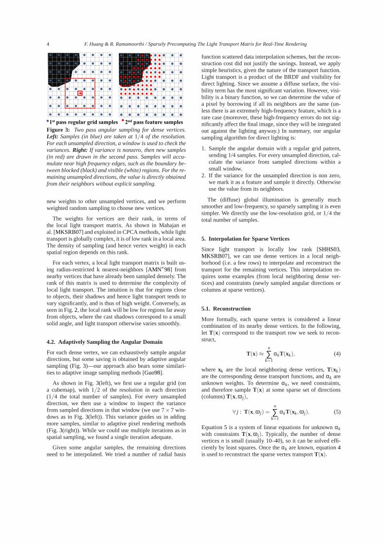
Figure 3: Two pass angular sampling for dense vertices.Left: Samples (in blue) are taken at1/4 of the resolution.For each unsampled direction, a window is used to check thevariances.Right: If variance is nonzero, then new samples(in red) are drawn in the second pass. Samples will accu-mulate near high frequency edges, such as the boundary be-tween blocked (black) and visible (white) regions. For the re-maining unsampled directions, the value is directly obtainedfrom their neighbors without explicit sampling.

new weights to other unsampled vertices, and we performweighted random sampling to choose new vertices.

The weights for vertices are their rank, in terms ofthe local light transport matrix. As shown in Mahajan etal. [MKSRB07] and exploited in CPCA methods, while lighttransport is globally complex, it is of low rank in a local area.The density of sampling (and hence vertex weight) in eachspatial region depends on this rank.

For each vertex, a local light transport matrix is built us-ing radius-restricted k nearest-neighbors [AMN∗98] fromnearby vertices that have already been sampled densely. Therank of this matrix is used to determine the complexity oflocal light transport. The intuition is that for regions closeto objects, their shadows and hence light transport tends tovary significantly, and is thus of high weight. Conversely, asseen in Fig.2, the local rank will be low for regions far awayfrom objects, where the cast shadows correspond to a smallsolid angle, and light transport otherwise varies smoothly.

4.2. Adaptively Sampling the Angular Domain

For each dense vertex, we can exhaustively sample angulardirections, but some saving is obtained by adaptive angularsampling (Fig.3)—our approach also bears some similari-ties to adaptive image sampling methods [Guo98].

As shown in Fig.3(left), we first use a regular grid (ona cubemap), with 1/2 of the resolution in each direction(1/4 the total number of samples). For every unsampleddirection, we then use a window to inspect the variancefrom sampled directions in that window (we use 7×7 win-dows as in Fig.3(left)). This variance guides us in addingmore samples, similar to adaptive pixel rendering methods(Fig. 3(right)). While we could use multiple iterations as inspatial sampling, we found a single iteration adequate.

Given some angular samples, the remaining directionsneed to be interpolated. We tried a number of radial basis

function scattered data interpolation schemes, but the recon-struction cost did not justify the savings. Instead, we applysimple heuristics, given the nature of the transport function.Light transport is a product of the BRDF and visibility fordirect lighting. Since we assume a diffuse surface, the visi-bility term has the most significant variation. However, visi-bility is a binary function, so we can determine the value ofa pixel by borrowing if all its neighbors are the same (un-less there is an extremely high-frequency feature, which isarare case (moreover, these high-frequency errors do not sig-nificantly affect the final image, since they will be integratedout against the lighting anyway.) In summary, our angularsampling algorithm for direct lighting is:

1. Sample the angular domain with a regular grid pattern,sending 1/4 samples. For every unsampled direction, cal-culate the variance from sampled directions within asmall window.

2. If the variance for the unsampled direction is non zero,we mark it as a feature and sample it directly. Otherwiseuse the value from its neighbors.

The (diffuse) global illumination is generally muchsmoother and low-frequency, so sparsely sampling it is evensimpler. We directly use the low-resolution grid, or 1/4 thetotal number of samples.

5. Interpolation for Sparse Vertices

Since light transport is locally low rank [SHHS03,MKSRB07], we can use dense vertices in a local neigh-borhood (i.e. a few rows) to interpolate and reconstruct thetransport for the remaining vertices. This interpolation re-quires some examples (from local neighboring dense ver-tices) and constraints (newly sampled angular directions orcolumns at sparse vertices).

5.1. Reconstruction

More formally, each sparse vertex is considered a linearcombination of its nearby dense vertices. In the following,let T(x) correspond to the transport row we seek to recon-struct,

T(x) ≈n

∑k=1

αkT(xk), (4)

where xk are the local neighboring dense vertices,T(xk)are the corresponding dense transport functions, andαk areunknown weights. To determineαk, we need constraints,and therefore sampleT(x) at some sparse set of directions(columns)T(x,ω j),

∀ j : T(x,ω j) =n

∑k=1

αkT(xk,ω j). (5)

Equation5 is a system of linear equations for unknownαkwith constraintsT(x,ω j). Typically, the number of denseverticesn is small (usually 10–40), so it can be solved effi-ciently by least squares. Once theαk are known, equation4is used to reconstruct the sparse vertex transportT(x).

F. Huang & R. Ramamoorthi / Sparsely Precomputing The Light Transport Matrix for Real-Time Rendering 5

While the least squares method solves equation5 well, thesolutions are sometimes not appropriate for reconstructingthe transport. Since we only use a small number of angularsamples, the least squares solution tends to over-fit the con-straints, causing large positive/negative weights, with mostlynon-zero values. Following [MKSRB07], if the local lighttransport is of low dimensionality, then a few samples shouldbe sufficient to form the bases and to describe the interpola-tion, leading to a sparse weighting vectorα.

Inspired by the compressive sensing literature, we haveobserved that better results can actually be obtained usingsparseL1 minimization (rather than least squares), using thefast algorithm in Kim et al. [KKL ∗07]. L1 reconstructionpreserves the sparse structure of light transport better, andleads to lower errors (results are shown later in Fig.6).

In order for the reconstruction to be good with a sparseset of directionsω j , it is crucial to sample useful angulardirections, and also choose appropriate local neighborsxk.

5.2. Choosing Angular Direction Samples (Columns)

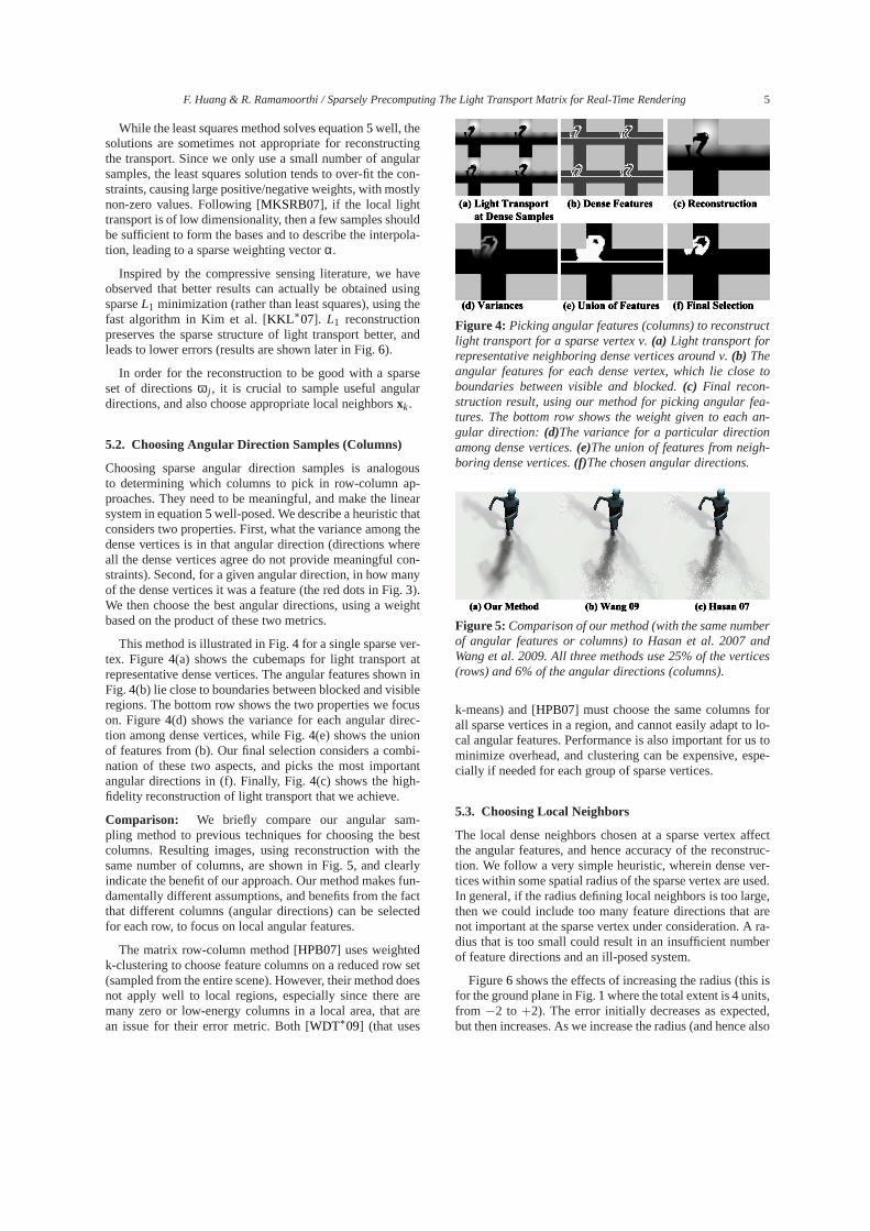
Choosing sparse angular direction samples is analogousto determining which columns to pick in row-column ap-proaches. They need to be meaningful, and make the linearsystem in equation5 well-posed. We describe a heuristic thatconsiders two properties. First, what the variance among thedense vertices is in that angular direction (directions whereall the dense vertices agree do not provide meaningful con-straints). Second, for a given angular direction, in how manyof the dense vertices it was a feature (the red dots in Fig.3).We then choose the best angular directions, using a weightbased on the product of these two metrics.

This method is illustrated in Fig.4 for a single sparse ver-tex. Figure4(a) shows the cubemaps for light transport atrepresentative dense vertices. The angular features showninFig.4(b) lie close to boundaries between blocked and visibleregions. The bottom row shows the two properties we focuson. Figure4(d) shows the variance for each angular direc-tion among dense vertices, while Fig.4(e) shows the unionof features from (b). Our final selection considers a combi-nation of these two aspects, and picks the most importantangular directions in (f). Finally, Fig.4(c) shows the high-fidelity reconstruction of light transport that we achieve.

Comparison: We briefly compare our angular sam-pling method to previous techniques for choosing the bestcolumns. Resulting images, using reconstruction with thesame number of columns, are shown in Fig.5, and clearlyindicate the benefit of our approach. Our method makes fun-damentally different assumptions, and benefits from the factthat different columns (angular directions) can be selectedfor each row, to focus on local angular features.

The matrix row-column method [HPB07] uses weightedk-clustering to choose feature columns on a reduced row set(sampled from the entire scene). However, their method doesnot apply well to local regions, especially since there aremany zero or low-energy columns in a local area, that arean issue for their error metric. Both [WDT∗09] (that uses

Figure 4: Picking angular features (columns) to reconstructlight transport for a sparse vertex v.(a) Light transport forrepresentative neighboring dense vertices around v.(b) Theangular features for each dense vertex, which lie close toboundaries between visible and blocked.(c) Final recon-struction result, using our method for picking angular fea-tures. The bottom row shows the weight given to each an-gular direction: (d)The variance for a particular directionamong dense vertices.(e)The union of features from neigh-boring dense vertices.(f)The chosen angular directions.

Figure 5: Comparison of our method (with the same numberof angular features or columns) to Hasan et al. 2007 andWang et al. 2009. All three methods use 25% of the vertices(rows) and 6% of the angular directions (columns).

k-means) and [HPB07] must choose the same columns forall sparse vertices in a region, and cannot easily adapt to lo-cal angular features. Performance is also important for us tominimize overhead, and clustering can be expensive, espe-cially if needed for each group of sparse vertices.

5.3. Choosing Local Neighbors

The local dense neighbors chosen at a sparse vertex affectthe angular features, and hence accuracy of the reconstruc-tion. We follow a very simple heuristic, wherein dense ver-tices within some spatial radius of the sparse vertex are used.In general, if the radius defining local neighbors is too large,then we could include too many feature directions that arenot important at the sparse vertex under consideration. A ra-dius that is too small could result in an insufficient numberof feature directions and an ill-posed system.

Figure6 shows the effects of increasing the radius (this isfor the ground plane in Fig.1 where the total extent is 4 units,from −2 to +2). The error initially decreases as expected,but then increases. As we increase the radius (and hence also

6 F. Huang & R. Ramamoorthi / Sparsely Precomputing The Light Transport Matrix for Real-Time Rendering0

.1

0.1

1

0.1

2

0.1

3

0.1

4

0.1

5

0.1

6

0.1

7

0.1

8

0.1

9

0.2

0.2

1

0.2

2

0.2

3

0.2

4

0.2

5

0.2

6

0.2

7

0.2

8

0.2

9

0.3

0.3

1

RM

S E

rro

r

Radius

RMS Error vs Radius

Least Squares L1 FULL

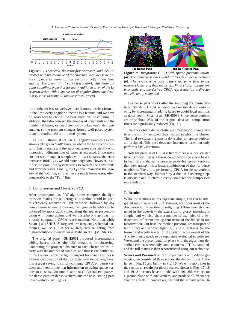
Figure 6: As expected, the error first decreases, and then in-creases with the radius used for choosing local dense neigh-bors. Sparse L1 minimization performs better than leastsquares. The green “Full” curve is a control, with dense an-gular sampling. Note that for many radii, the error of the L1reconstruction with a sparse set of angular directions (red)is very close to using all the directions (green).

the number of bases), we have more features to select from—in the limit every angular direction is a feature, and we haveno good way to choose the best directions or columns. Inaddition, the ratio between the number of constraints and thenumber of bases, or coefficientsαk (unknowns), also getssmaller, so the problem changes from a well-posed systemto an ill-conditioned or ill-posed system.

As Fig. 6 shows, if we use all angular samples as con-straints (the green “Full” line), we obtain the best reconstruc-tion. This is stable and the error decreases consistently withincreasing radius/number of bases as expected. If we use asmaller set of angular samples with least squares, the errordecreases initially as we add more neighbors. However, at aninflection point, the system starts to over-fit the constraintsand error increases. Finally, theL1 solver maintains the spar-sity of the solution, so it achieve a much lower error, oftencomparable to the “Full” line.

6. Compression and Clustered PCA

After precomputation, PRT algorithms compress the lighttransport matrix for relighting. Our method could be usedto efficiently reconstruct light transport, followed by anycompression scheme. However, even greater benefits can beobtained by more tightly integrating the sparse precompu-tation with compression, and we describe one approach todirectly compute a CPCA representation. Note that whileSloan et al. [SHHS03] targeted low-frequency spherical har-monics, we use CPCA for all-frequency relighting fromhigh-resolution cubemaps, as in Mahajan et al. [MKSRB07].

The original paper [SHHS03] proposed incrementallyadding bases, besides the LBG iterations for clustering.Computing the projected distance to each cluster scales lin-early with the number of samples, and thus is the bottleneckof the system. Since the light transport for sparse verticesisa linear combination of that for their local dense neighbors,it is a great saving to simply compute CPCA on dense ver-tices, and then utilize that information to assign sparse ver-tices to clusters. Our modification to CPCA has two passes:the dense pass on dense vertices, and the re-clustering passon all vertices (see Fig.7).

Figure 7: Integrating CPCA with sparse precomputation.(a): The dense pass does standard CPCA on dense vertices(b): The re-clustering pass assigns sparse vertices to thenearest cluster and then reclusters. Final cluster assignmentis smooth, and the desired CPCA representation is directlyand efficiently computed.

The dense pass works after the sampling for dense ver-tices. Standard CPCA is performed on the dense verticesonly, by incrementally adding bases to avoid local minima,as described in Sloan et al. [SHHS03]. Since dense verticesare only about 25% of the original data set, computationtimes are significantly reduced (Fig.11).

Once we obtain dense clustering information, sparse ver-tices are simply assigned their nearest neighboring cluster.The final re-clustering pass is done after all sparse verticesare assigned. This pass does not increment bases but onlyperforms LBG iterations.

Note the premise of CPCA is that vertices in a local clusterhave transport that is a linear combinations of a few bases.In fact, this is the same premise made for sparse vertices,that their transport is a linear combination of that for denseneighbors. Therefore, performing CPCA for dense verticesin the standard way, followed by a final re-clustering step,is adequate and in effect directly computes the compressedrepresentation.

7. Results

While the methods in this paper are simple, and can be inte-grated into a variety of PRT systems, we focus most of thediscussion in this section on relighting diffuse geometry.Asnoted in the overview, the extension to glossy materials issimple, and we also show a number of examples of view-dependent reflectance using four terms of the BRDF in-outfactorization. Our baseline method precomputes transportofboth direct and indirect lighting, using a raytracer for theformer and a path tracer for the latter. Each element of theT(x,ω) matrix needs to be separately evaluated in software.We extend the precomputation phase with the algorithms de-scribed earlier, where only some elements ofT are sampled,and the full matrix is then reconstructed using our technique.

Scenes and Parameters:For experiments with diffuse ge-ometry, we considered three scenes: the dancer in Fig.1, thehorse in Fig.15and bunny in Fig.16. We will report later inthe section on results for glossy scenes, shown in Figs.17, 18and19. All scenes have a model with 10k–35k vertices ona ground plane with 30k vertices, and produce all-frequencyshadow effects in contact regions and the ground plane. In

F. Huang & R. Ramamoorthi / Sparsely Precomputing The Light Transport Matrix for Real-Time Rendering 7

Scene Mesh Num.

Vert.

Dense

Vert.

Radius Num.

Feat.

Num.

Clusters

Num

Basis

Dancer Model 9,971 2500 0.2 350 50 24

Ground 29,241 6000 0.2 350 100 24

Horse Model 8,431 2100 0.2 350 50 24

Ground 29,241 6000 0.2 350 120 24

Bunny Model 35,103 8850 0.2 350 70 24

Ground 29,241 6000 0.2 350 120 24

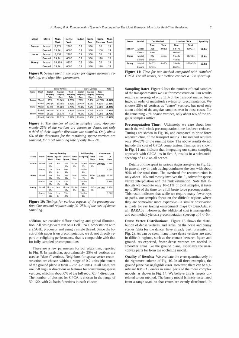
Figure 8: Scenes used in the paper for diffuse geometry re-lighting, and algorithm parameters.

Dense Ver�ces Sparse Ver�ces Total

Scene Mesh Spa�al

Sampling

Rate

Angular

Sampling

Rate

Total

Sampling

Rate

Spa�al

Sampling

Rate

Angular

Sampling

Rate

Total

Sampling

Rate

Dancer Model 25% 31.06% 7.76% 75% 5.7% 4.275% 12.04%

Ground 20.52% 30.78% 6.32% 79.48% 5.7% 4.53% 10.85%

Horse Model 24.9% 31.26% 7.78% 75.1% 5.7% 4.28% 12.06%

Ground 20.52% 31.32% 6.42% 79.48% 5.7% 4.53% 10.95%

Bunny Model 25.2% 29.87% 7.53 74.8% 5.7% 4.26% 11.79%

Ground 20.52% 29.31% 6.01% 79.48% 5.7% 4.53% 10.54%

Figure 9: The number of sparse samples used. Approxi-mately 25% of the vertices are chosen as dense, but onlya third of their angular directions are sampled. Only about6% of the directions for the remaining sparse vertices aresampled, for a net sampling rate of only 10–12%.

Sparsely Sampling Full Sampling Comparison

Scene Mesh Dense

Time

Sparse

Time

Dense+

Sparse

Total

Time

Sampling Total

Time

Time

Ra!o

L2

Error

Dancer Model 16m

32s

8m 24m

32s

1h15m

18s

2h13m

35s

5h40m

19s

20.95% 7.43%

Ground 22m

40s

28m

6s

50m

46s

3h26m

44s

1.72%

Horse Model 10m

29s

6m

26s

16m

55s

54m

9s

1h46m

7s

4h2m

22s

22.35% 10.2%

Ground 15m

55s

21m

18s

37m

14s

2h16m

15s

1.61%

Bunny Model 1h32m

18s

56m 2h28m

18s

3h25m

55s

9h52m

47s

13h7m

57s

26.14% 2.86%

Ground 26m

31s

31m

6s

57m

37s

3h15m

10s

0.79%

Figure 10: Timings for various aspects of the precomputa-tion. Our method requires only 20–25% of the cost of densesampling.

addition, we consider diffuse shading and global illumina-tion. All timings were run on a Dell T7400 workstation witha 2.5GHz processor and using a single thread. Since the fo-cus of this paper is on precomputation, we do not directly re-port on relighting performance, that is comparable with thatfor fully sampled precomputations.

There are a few parameters for our algorithm, reportedin Fig. 8. In particular, approximately 25% of vertices areused as “dense” vertices. Neighbors for sparse vertex recon-struction are chosen within a range of 0.2 units (the extentof the ground plane is from−2 to+2 units). In all cases, weuse 350 angular directions or features for constraining sparsevertices, which is about 6% of the full set of 6144 directions.The number of clusters for CPCA is chosen in the range of50–120, with 24 basis functions in each cluster.

Scene Model Our Method Standard CPCA Speed Up

Time Total Time Total

Dancer Model 32s 3m37s 6m47s 45m31s 12.6x

Ground 3m5s 38m44s

Horse Model 27s 4m6s 5m40s 51m48s 12.6x

Ground 3m39s 46m8s

Bunny Model 2m37s 6m20s 38m3s 1h20m57s 12.8x

Ground 3m43s 42m54s

Figure 11: Time for our method compared with standardCPCA. For all scenes, our method enables a12× speed up.

Sampling Rate: Figure9 lists the number of total samplesof the transport matrix we use for reconstruction. Our resultsrequire an average of only 11% of the transport matrix, lead-ing to an order of magnitude savings for precomputation. Wechoose 25% of vertices as “dense” vertices, but need onlyabout a third of the angular samples even in those cases. Forthe remaining 75% sparse vertices, only about 6% of the an-gular samples suffice.

Precomputation Time: Ultimately, we care about howmuch the wall clock precomputation time has been reduced.Timings are shown in Fig.10, and compared to brute forcereconstruction of the transport matrix. Our method requiresonly 20–25% of the running time. The above results do notinclude the cost of CPCA compression. Timings are shownin Fig. 11 and indicate that integrating our sparse samplingapproach with CPCA, as in Sec.6, results in a substantialspeedup of 12× on all scenes.

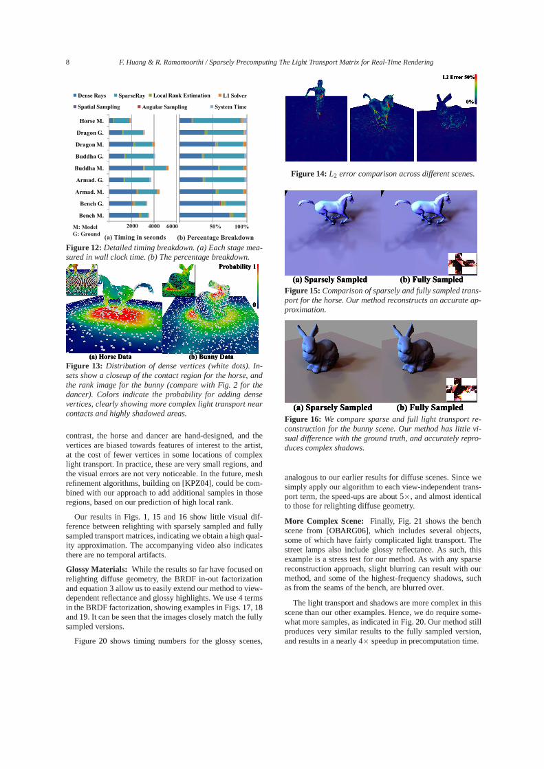
Details of time spent in various stages are given in Fig.12.In general, ray or path tracing dominates the cost with about90% of the total time. The overhead for reconstruction isonly about 10% and mostly involves theL1 solver for sparsevertex interpolation and the rank estimation. Note that al-though we compute only 10–11% of total samples, it takesup to 20% of the time for a full brute force precomputation.This result indicates that while we require many fewer raysor paths, our samples focus on the difficult regions wherethey are somewhat more expensive—a similar observationis made for ray tracing environment maps by Ben-Artzi etal. [BARA06]. However, the additional cost is manageable,and our method yields a precomputation speedup of 4×–5×.

Dense Vertex Distributions: Figure 13 shows the distri-bution of dense vertices, and ranks, on the horse and bunnyscenes (data for the dancer have already been presented inFig. 2). As can be seen, many more dense vertices are usedin difficult regions, such as the contact between figure andground. As expected, fewer dense vertices are needed insmoother areas like the ground plane, especially the near-convex parts far from the occluding model.

Quality of Results: We evaluate the error quantitatively inthe rightmost column of Fig.10. In all three examples, theground plane has negligible error. However, there can be sig-nificant RMSL2 errors in small parts of the more complexmodels, as shown in Fig.14. We believe this is largely un-related to our method. The bunny model is finely tessellatedfrom a range scan, so that errors are evenly distributed. In

8 F. Huang & R. Ramamoorthi / Sparsely Precomputing The Light Transport Matrix for Real-Time Rendering

Bench M.

Bench G.

Armad. M.

Armad. G.

Buddha M.

Buddha G.

Dragon M.

Dragon G.

Horse M.

Dense Rays

Angular Sampling

Local Rank Estimation

Spatial Sampling

SparseRay L1 Solver

System Time

M: Model

G: Ground(a) Timing in seconds (b) Percentage Breakdown

50% 100%2000 4000 6000

Figure 12: Detailed timing breakdown. (a) Each stage mea-sured in wall clock time. (b) The percentage breakdown.

Figure 13: Distribution of dense vertices (white dots). In-sets show a closeup of the contact region for the horse, andthe rank image for the bunny (compare with Fig.2 for thedancer). Colors indicate the probability for adding densevertices, clearly showing more complex light transport nearcontacts and highly shadowed areas.

contrast, the horse and dancer are hand-designed, and thevertices are biased towards features of interest to the artist,at the cost of fewer vertices in some locations of complexlight transport. In practice, these are very small regions,andthe visual errors are not very noticeable. In the future, meshrefinement algorithms, building on [KPZ04], could be com-bined with our approach to add additional samples in thoseregions, based on our prediction of high local rank.

Our results in Figs.1, 15 and 16 show little visual dif-ference between relighting with sparsely sampled and fullysampled transport matrices, indicating we obtain a high qual-ity approximation. The accompanying video also indicatesthere are no temporal artifacts.

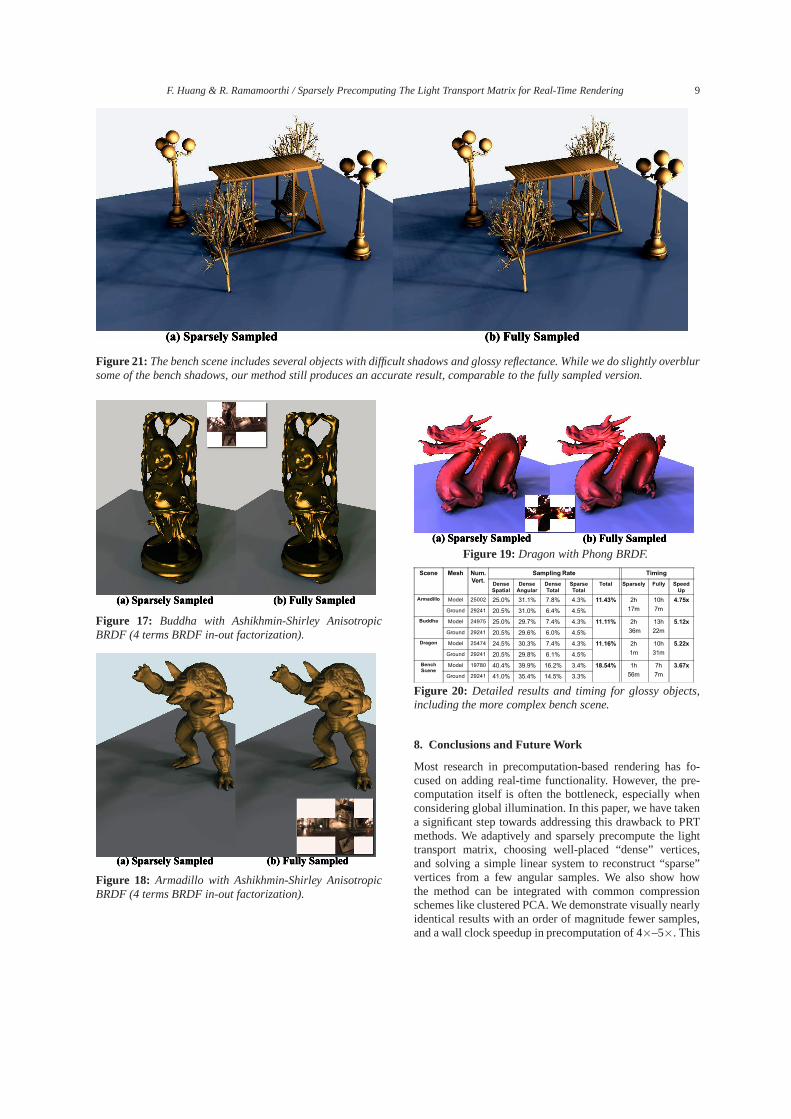
Glossy Materials: While the results so far have focused onrelighting diffuse geometry, the BRDF in-out factorizationand equation3 allow us to easily extend our method to view-dependent reflectance and glossy highlights. We use 4 termsin the BRDF factorization, showing examples in Figs.17, 18and19. It can be seen that the images closely match the fullysampled versions.

Figure 20 shows timing numbers for the glossy scenes,

Figure 14: L2 error comparison across different scenes.

Figure 15: Comparison of sparsely and fully sampled trans-port for the horse. Our method reconstructs an accurate ap-proximation.

Figure 16: We compare sparse and full light transport re-construction for the bunny scene. Our method has little vi-sual difference with the ground truth, and accurately repro-duces complex shadows.

analogous to our earlier results for diffuse scenes. Since wesimply apply our algorithm to each view-independent trans-port term, the speed-ups are about 5×, and almost identicalto those for relighting diffuse geometry.

More Complex Scene: Finally, Fig. 21 shows the benchscene from [OBARG06], which includes several objects,some of which have fairly complicated light transport. Thestreet lamps also include glossy reflectance. As such, thisexample is a stress test for our method. As with any sparsereconstruction approach, slight blurring can result with ourmethod, and some of the highest-frequency shadows, suchas from the seams of the bench, are blurred over.

The light transport and shadows are more complex in thisscene than our other examples. Hence, we do require some-what more samples, as indicated in Fig.20. Our method stillproduces very similar results to the fully sampled version,and results in a nearly 4× speedup in precomputation time.

F. Huang & R. Ramamoorthi / Sparsely Precomputing The Light Transport Matrix for Real-Time Rendering 9

Figure 21: The bench scene includes several objects with difficult shadows and glossy reflectance. While we do slightly overblursome of the bench shadows, our method still produces an accurate result, comparable to the fully sampled version.

Figure 17: Buddha with Ashikhmin-Shirley AnisotropicBRDF (4 terms BRDF in-out factorization).

Figure 18: Armadillo with Ashikhmin-Shirley AnisotropicBRDF (4 terms BRDF in-out factorization).

Figure 19: Dragon with Phong BRDF.

Scene Mesh Num.

Vert.

Sampling Rate Timing

Dense

Spatial

Dense

Angular

Dense

Total

Sparse

Total

Total Sparsely Fully Speed

Up

Armadillo Model 25002 25.0% 31.1% 7.8% 4.3% 11.43% 2h

17m

10h

7m

4.75x

Ground 29241 20.5% 31.0% 6.4% 4.5%

Buddha Model 24975 25.0% 29.7% 7.4% 4.3% 11.11% 2h

36m

13h

22m

5.12x

Ground 29241 20.5% 29.6% 6.0% 4.5%

Dragon Model 25474 24.5% 30.3% 7.4% 4.3% 11.16% 2h

1m

10h

31m

5.22x

Ground 29241 20.5% 29.8% 6.1% 4.5%

Bench

SceneModel 19780 40.4% 39.9% 16.2% 3.4% 18.54% 1h

56m

7h

7m

3.67x

Ground 29241 41.0% 35.4% 14.5% 3.3%

Figure 20: Detailed results and timing for glossy objects,including the more complex bench scene.

8. Conclusions and Future Work

Most research in precomputation-based rendering has fo-cused on adding real-time functionality. However, the pre-computation itself is often the bottleneck, especially whenconsidering global illumination. In this paper, we have takena significant step towards addressing this drawback to PRTmethods. We adaptively and sparsely precompute the lighttransport matrix, choosing well-placed “dense” vertices,and solving a simple linear system to reconstruct “sparse”vertices from a few angular samples. We also show howthe method can be integrated with common compressionschemes like clustered PCA. We demonstrate visually nearlyidentical results with an order of magnitude fewer samples,and a wall clock speedup in precomputation of 4×–5×. This

10 F. Huang & R. Ramamoorthi / Sparsely Precomputing The Light Transport Matrix for Real-Time Rendering

has the potential to enable new approaches to rapid prototyp-ing of scenes for lighting design or gaming environments.

In the future, we would like to leverage recent advancesin GPU-based global illumination, to develop a hardware-accelerated precomputation pipeline. We envisage a systemwhere the precomputation phase is interactive or takes onlya few seconds, greatly reducing the barrier to PRT methods.We would also like to gain a deeper theoretical understand-ing into what samples of the transport matrix enable the bestreconstructions, and how these vary for different types ofscenes. Finally, estimation of variants of the transport ma-trix is also a challenge in offline many-light rendering andappearance acquisition, and we believe the insights in thispaper hold promise for those domains as well.

Acknowledgements

This work was supported in part by NSF CAREER grantIIS-0924968 and ONR PECASE grant N00014-09-1-0741,as well as equipment and generous support from Intel,NVIDIA, Adobe, and Pixar.

References

[AMN ∗98] ARYA S., MOUNT D., NETANYAHU N., SILVER-MAN R., WU A.: An optimal algorithm for approximate nearestneighbor searching in fixed dimensions.Journal of the ACM 45,6 (1998), 891–923.

[BARA06] BEN-ARTZI A., RAMAMOORTHI R., AGRAWALAM.: Efficient shadows from sampled environment maps.Journalof Graphics Tools 11, 1 (2006), 13–36.

[CRT06] CANDES E., ROMBERGJ., TAO T.: Stable signal recov-ery from incomplete and inaccurate measurements.Communica-tions of Pure and Applied Mathematics 59, 8 (2006), 1207–1223.

[CT06] CANDES E., TAO T.: Near optimal signal recovery fromrandom projections: Universal encoding strategies?IEEE Trans-actions on Information Theory 52, 12 (2006), 5406–5425.

[DAG95] DORSEY J., ARVO J., GREENBERG D.: Interactivedesign of complex time-dependent lighting.IEEE ComputerGraphics and Applications 15, 2 (1995), 26–36.

[DMM08] D RINEAS P., MAHONEY M., MUTHUKRISHNAN S.:Relative-error CUR matrix decompositions.SIAM J. MatrixAnal. Appl. 30, 2 (2008), 844–881.

[Guo98] GUO B.: Progressive radiance evaluation using direc-tional coherence maps. InSIGGRAPH 98(1998), pp. 255–266.

[HPB06] HASAN M., PELLACINI F., BALA K.: Direct to indirecttransfer for cinematic relighting.ACM Transactions on Graphics(SIGGRAPH 06) 25, 3 (2006), 1089–1097.

[HPB07] HASAN M., PELLACINI F., BALA K.: Matrix row-column sampling for the many-light problem.ACM Transactionson Graphics (Proc. SIGGRAPH 07) 26, 3 (2007), Article 26.

[KG09] KRIVANEK J., GAUTRON P.: Practical Global Illumina-tion with Irradiance Caching. Morgan and Claypool, 2009.

[KKL ∗07] KIM S., KOH K., LUSTIG M., BOYD S.,GORINEVSKY D.: An interior-point method for large-scaleL1regularized least squares.IEEE Journal on Selected Topics inSignal Processing 1, 4 (2007), 606–617.

[KPZ04] KRIVANEK J., PATTANAIK S., ZARA J.: Adaptive meshsubdivision for precomputed radiance transfer. InSCCG 04: Pro-ceedings of the 20th spring conference on Computer graphics(2004), pp. 106–111.

[KTHS06] KONTKANEN J., TURQUIN E., HOLZSCHUCH N.,SILLION F.: Wavelet radiance transport for real-time indirectlighting. In EuroGraphics Symposium on Rendering 06(2006),pp. 161–172.

[LSSS04] LIU X., SLOAN P., SHUM H., SNYDER J.: All-frequency precomputed radiance transfer for glossy objects. InEuroGraphics Symposium on Rendering 04(2004), pp. 337–344.

[LZT∗08] LEHTINEN J., ZWICKER M., TURQUIN E., KONTKA-NEN J., DURAND F., SILLION F., AILA T.: A meshless hierar-chical representation for light transport.ACM Transactions onGraphics (Proc. SIGGRAPH 08) 27, 3 (2008), Article 37, 1–9.

[MKSRB07] MAHAJAN D., KEMELMACHER-SHLIZERMAN I.,RAMAMOORTHI R., BELHUMEUR P.: A theory of locally lowdimensional light transport. ACM Transactions on Graphics(Proc. SIGGRAPH 07) 26, 3 (2007), 62.

[NRH03] NG R., RAMAMOORTHI R., HANRAHAN P.: All-frequency shadows using non-linear wavelet lighting approxima-tion. ACM Transactions on Graphics (Proc. SIGGRAPH 03) 22,3 (2003), 376–381.

[NRH04] NG R., RAMAMOORTHI R., HANRAHAN P.: Tripleproduct wavelet integrals for all-frequency relighting.ACMTransactions on Graphics (Proc. SIGGRAPH 04) 23, 3 (2004),475–485.

[NSD94] NIMEROFF J., SIMONCELLI E., DORSEYJ.: Efficientre-rendering of naturally illuminated environments. InEuro-Graphics Workshop on Rendering 94(1994), pp. 359–373.

[OBARG06] OVERBECK R., BEN-ARTZI A., RAMAMOORTHIR., GRINSPUNE.: Exploiting temporal coherence for incremen-tal all-frequency relighting. InEuroGraphics Symposium on Ren-dering(2006), pp. 151–160.

[PML∗09] PEERS P., MAHAJAN D., LAMOND B., GHOSH A.,MATUSIK W., RAMAMOORTHI R., DEBEVEC P.: Compressivelight transport sensing.ACM Transactions on Graphics 28, 1(2009), Article 3, pages 1–18.

[Ram09] RAMAMOORTHI R.: Precomputation-Based Rendering.NOW Publishers Inc, 2009.

[SD09] SEN P., DARABI S.: Compressive Dual Photography.Computer Graphics Forum (EUROGRAPHICS 09) 28, 2 (2009),609 – 618.

[SHHS03] SLOAN P., HALL J., HART J., SNYDER J.: Clusteredprincipal components for precomputed radiance transfer.ACMTransactions on Graphics (Proc. SIGGRAPH 03) 22, 3 (2003),382–391.

[SKS02] SLOAN P., KAUTZ J., SNYDER J.: Precomputed radi-ance transfer for real-time rendering in dynamic, low-frequencylighting environments. ACM Transactions on Graphics (SIG-GRAPH 02) 21, 3 (2002), 527–536.

[WDT∗09] WANG J., DONG Y., TONG X., L IN Z., GUO B.:Kernel nystrom method for light transport.ACM Transactionson Graphics (Proc. SIGGRAPH 09) 28, 3 (2009).

[WTL04] WANG R., TRAN J., LUEBKE D.: All-frequency re-lighting of non-diffuse objects using separable BRDF approx-imation. In EuroGraphics Symposium on Rendering(2004),pp. 345–354.