1

Sparse Representation-Based SAR Imaging Sadegh Samadi 1, Müjdat Çetin 2, Mohammad Ali Masnadi-Shirazi 1

1School of Electrical and Computer Engineering, Shiraz University, Zand Street, 71348-51154 Shiraz, Iran.

2Faculty of Engineering and Natural Sciences, Sabanci University, Tuzla, 34956 Istanbul, Turkey. ssamadi@shirazu.ac.ir , mcetin@sabanciuniv.edu , masnadi@shirazu.ac.ir

ABSTRACT

There is increasing interest in using synthetic aperture radar (SAR) images in automated target recognition

and decision-making tasks. The success of such tasks depends on how well the reconstructed SAR images

exhibit certain features of the underlying scene. Based on the observation that typical underlying scenes

usually exhibit sparsity in terms of such features, we develop an image formation method which formulates

the SAR imaging problem as a sparse signal representation problem. Sparse signal representation, which has

mostly been exploited in real-valued problems, has many capabilities such as superresolution and feature

enhancement for various reconstruction and recognition tasks. However, for problems of complex-valued

nature, such as SAR, a key challenge is how to choose the dictionary and the representation scheme for

effective sparse representation. Since we are usually interested in features of the magnitude of the SAR

reflectivity field, our new approach is designed to sparsely represent the magnitude of the complex-valued

scattered field. This turns the image reconstruction problem into a joint optimization problem over the

representation of magnitude and phase of the underlying field reflectivities. We develop the mathematical

framework for this method and propose an iterative solution for the corresponding joint optimization problem.

Our experimental results demonstrate the superiority of this method over previous approaches in terms of

both producing high quality SAR images as well as exhibiting robustness to uncertain or limited data.

Keywords: synthetic aperture radar, sparse signal representation, complex-valued imaging, overcomplete

dictionary, feature enhancement, image reconstruction, optimization.

1. INTRODUCTION

Synthetic aperture radar (SAR) is an active microwave sensor which is able to produce high-resolution

images of the earth’s surface at any time. With day and night capability and all weather operation, SAR is one

2

of the most promising remote sensing modalities. SAR makes use of a sensor carried on an airborne or

spaceborne platform, transmitting microwave pulses towards an area of interest on the earth, and receives the

reflected signal. This signal first undergoes some pre-processing tasks including a demodulation process. The

SAR image formation problem is the problem of reconstruction of a spatial reflectivity distribution of the

scene from the pre-processed SAR returns. In this paper, we focus on spotlight-mode SAR [1], although the

proposed ideas are not limited to a specific mode.

Recently there has been significant and increasing interest in using SAR images in automated target

recognition and decision-making tasks. The success of such tasks depends on how well the reconstructed SAR

images exhibit certain features of the underlying scene. The conventional approach for spotlight-mode SAR

image formation is the polar format algorithm (PFA) [1], which is based on the premise of clean, full-

aperture, full-bandwidth data. This method has no explicit mechanism to counter any imperfection including

noise in the data, and also suffers from important shortcomings, such as resolution limitation to system

bandwidth, speckle, and sidelobe artifacts. These limitations make it difficult to use conventionally

reconstructed SAR images for robust recognition and decision-making tasks.

Based on the observation that typical underlying scenes usually exhibit sparsity in terms of certain features of

interest, we develop an image formation method which formulates the SAR imaging problem as a sparse

signal representation problem. Sparse signal representation, which has mostly been exploited in real-valued

problems, offers many advantages such as superresolution and feature enhancement for various reconstruction

and recognition tasks. Recent work on feature-enhanced SAR image formation based on nonquadratic

regularization [2] has ties to sparse representation. In particular, one interpretation of the technique in [2]

involves sparse representation with some fixed and specific dictionaries which makes it useful for scenes

containing a limited set of specific feature types. This is only an interpretation as the (fixed) dictionaries

involved in the approach are only implicit, and the optimization problem is formulated over the reflectivities

rather than the sparse representation coefficients. The method proposed here extends and generalizes the

approach in [2] to sparse representation with arbitrary, general dictionaries to handle general scenes

containing any type of features. This is achieved by explicitly formulating the SAR image formation problem

as a sparse representation problem with arbitrary dictionaries.

3

A key challenge for exploiting sparse representation (SR) in complex-valued problems such as SAR imaging

is how to choose the dictionary and the representation scheme. In this paper we develop a mathematical

framework to deal with these issues. In particular, we apply sparse representation on the magnitude of the

complex-valued scattered field which leads to a joint optimization problem over the representation of

magnitude and phase of the underlying field reflectivities. The framework leads to an iterative algorithm for

solving the joint optimization problem. To demonstrate our approach, we have used some sample dictionaries,

including multi-resolution dictionaries, as well as dictionaries adapted to the shapes of the likely objects in the

scene. However, this framework has the capability of using any appropriate dictionary for the particular

application of interest. The rest of this paper is organized as follows. In Section 2 details of SR-based SAR

imaging are presented. In Section 3 experimental results on various SAR images are presented to demonstrate

the effectiveness of our approach. Eventually, some concluding remarks are made in Section 4.

2. SPARSE REPRESENTATION FRAMEWORK FOR SAR IMAGE FORMATION

Sparse signal representation has successfully been used for solving inverse problems in a variety of

applications. It has many capabilities for various reconstruction and recognition tasks; however, it has mostly

been used in real-valued problems. Due to the complex-valued and potentially random phase nature of the

reflectivities in SAR, our approach is designed to sparsely represent the magnitude of the complex-valued

scattered field where in its features we are interested.

2.1 OBSERVATION MODEL

We use an observation model for spotlight-mode SAR imaging motivated by the tomographic formulation of

SAR [3]. Data are collected using a radar sensor traversing a flight path with an antenna boresight realigned

continually to point at a fixed ground patch. The most commonly used transmitting pulse in SAR is a linear

FM chirp pulse )( 20)( ttjets μω += for |t|≤Tp/2 and zero otherwise. Here 0ω is the carrier frequency and 2μ is

the so-called chirp rate. SAR transmits pulses at positions of equal angular increments. The backscattered

signal from the scene is mixed with a reference chirp and passed through a low-pass filter. Typically, it is

assumed that the distance from radar to the center of the scene (Rθ) is much greater than the ground patch

radius (L). In this case the demodulated observed signal is given by [1,2]:

4

{ } dydxyxtjyxftsLyx

b ∫∫≤+

+Ω−=222

)sincos()(exp),(),( θθθ (1)

Where ( )))/2((22)( 0 cRtc

t θμω −+=Ω denotes the radial spatial frequency, f(x,y) is the complex-valued

reflectivity field (the unknown image), and c is the speed of light. Note that ),( ts ib θ is a finite slice through

the 2D Fourier transform of the field reflectivity at angle iθ , and is usually referred to as the phase histories.

A discretized version of Equation (1) can be written as [2]:

fCS =b (2)

where ttttb M

][21 θθθ sssS L= is a vector of sampled phase histories, tttt

M][

21 θθθ cccC L= is a discretized

approximation to the observation kernel in (1), and f a vector of unknown sampled reflectivity image. Using

the projection slice theorem [4], the observed phase histories can also be written as [2]:

{ }∫− Ω−=L

Lb duutjugts )(exp),(),( θθ (3)

where ),( ug iθ is the projection of f(x,y) at angle iθ . Using (1) and (3) a discrete relation between the field f

and the projections g can be obtained as [2]:

fHfCFSFg === −− 11b (4)

Where 1−F is a block diagonal matrix with each block performing an IDFT on each iθs , and H represents a

complex-valued discrete SAR projection operator. The data g in (4) are called range profiles. In the presence

of noise, the range profile observation model becomes:

y = H f + n (5)

where n is the additive observation noise. A similar phase history observation model can be obtained based on

Equation (2), however the model in (5) has computational benefits due to the approximately sparse nature of

H [2]. A convolutional linear model can also be defined by replacing y in (5) with a conventionally

reconstructed image, and letting H be replaced with a matrix with each row containing a spatially shifted

version of the corresponding point spread function (PSF) stacked as a row vector [5]. This form provides

some computational (especially memory) advantages as the matrix vector operations can be performed

through convolutions.

5

2.2 SPARSE REPRESENTATION SCHEME

In this subsection we present our sparse representation framework that effectively deals with the complex-

valued nature of the SAR signal and can be used for enhanced SAR image formation. Since we are usually

interested in features of the magnitude of the SAR signal, our new approach is designed to sparsely represent

the magnitude of the complex-valued scattered field. Thus, we consider:

Φαf = (6)

where Φ is an appropriate dictionary for our application that can sparsely represent the magnitude of the

scattered field (or simply the scene) in terms of the features of interest, and α is the vector of representation

coefficients. For any complex-valued vector f we can write fPf = , where { }ijφediag=P is a diagonal

matrix, and φi represents the unknown phase of image vector element (f)i. Thus, we can rewrite the

observation model as:

nαΦPHnfPHnfHy +=+=+= (7)

If we knew P (or phases of the elements of the unknown image vector), using an atomic decomposition

technique such as an extension of basis pursuit denoising [6], we could find an estimate of α , and hence the

magnitude image of the unknown scene itself, as follows:

ppλ ααΦPHyα

α+−= 2

2minargˆ (8)

where p⋅ denotes the pl -norm, and λ is a positive real scalar parameter. Note that the 2l -norm term in (8)

is related to the assumption that noise is zero mean white Gaussian1. Also note that the perfect sparsity

condition term would involve an 0l -norm which would lead to a combinatorial, hard-to-solve problem.

However, it is shown that for fields that admit a sparse enough representation, the pl -norm with p ≤ 1, as we

use here, also leads to the sparsest of all representations under certain conditions [7-11].

However, the difficulty in solving the optimization problem in (8) is that we don't know the phase terms of the

image vector elements and hence the matrix P. We propose the following joint optimization approach to

overcome this problem:

1 For colored noise, a weighted norm can be used in our data term.

6

a. Start with an initial estimate of f that could be its conventional reconstruction. Using this f, an initial

estimate of the image phase matrix, P can be obtained.

b. Using this estimate of P, the optimization problem in (8) can be solved and a new estimate of α can be

obtained.

c. Using the new estimate of α , the new estimate of f can be produced from (6). Now, a new estimate of the

phase matrix P should be found. To do this rewrite the observation model as:

nβBHnfPHy +=+= (9)

where matrix { }i)(diag fB= and β is a vector formed by stacking the diagonal elements of matrix P, hence it

contains the unknown phase terms. An estimate of β can be obtained through the following estimator:

ii ∀=−= ,1)(tosubjectminargˆ 22 ββBHyβ

β (10)

where the unconstrained part of (10) is both the maximum likelihood (ML) and the minimum variance

unbiased (MVU) estimator of β [12]. This is due to the assumption that the observation noise is independent

identically distributed complex Gaussian noise, which is the most commonly used statistical model for radar

measurement noise [13,14], and also the linearity of the observation model in (9). However, the prior

information on β introduces a constraint to the problem which results in the optimization problem in (10). For

most of the SAR scenes phase of the reflectivity at a certain location could be modeled as random, with a

uniform probability density function, and independent of the phase at other locations [15]. Assuming this

prior information, it is also interesting to investigate the Bayesian estimation approach for this problem. In

particular, the maximum a posteriori (MAP) estimator is considered here which is obtained as follows:

)(p)|(pmaxargˆMAP ββyβ

β= (11)

Since the magnitude of any vector element (β)i is a constant independent of its phase, p(β) can be written as

(see appendix A) : ∏=

∠−=2

1))(U(1))(δ()(p

N

iii βββ (12)

where )U(⋅ is a uniform function over [-π,π], )δ(⋅ is delta function that can be considered as a uniform

function over [-ε,ε] for a very small value of ε, and N2 is the number of elements of vector β for an image of

size N×N. Also, p(y|β) is a complex Gaussian pdf. Note that p(β) is equal to a constant when all the values of

7

|(β)i| terms are in the vicinity of 1 and all the phase terms ∠(β)i are in the interval of [-π,π]. Otherwise p(β) is

equal to zero. Thus, the maximum of (11) occurs when the first term on the right side is maximum with the

constraint that all the magnitude values of (β)i terms are in the vicinity of 1 and all their phases are in the

interval of [-π,π]. Therefore, it can be easily shown that the constrained estimator in (10) is also the MAP

estimator of β, whenever all phases of the solution are considered to be in the interval of [-π,π].

Using N2 Lagrange multipliers the constrained problem in (10) can be replaced with the following

unconstrained problem: ∑=

−′+−=2

1ii

22 1))((minargˆ

N

iλ ββBHyβ

β (13)

Note that the N2 constraints ii ∀= ,1)(β are equivalent to the one constraint 01))((2

1

2 =−∑=

N

iiβ , since the

summation of some nonnegative real terms will be equal to zero if and only if all of them are equal to zero.

This reduces the optimization problem in (13) to the following problem which is much more tractable:

∑=

−′+−=2

1

222 1))((minargˆ

N

iiλ ββBHyβ

β

122

22 2minarg βββBHy

βλλ ′−′+−= (14)

Solving this optimization problem produces a new estimate of the phase vector β and hence the matrix

{ }i)(diag βP = .

d. Go back to step (b) and repeat this loop until δ<−+ 2

2)(2

2)()1( |ˆ||ˆ||ˆ| nnn fff , where δ is a small positive

real constant, and )(|ˆ| nf is the estimate of f in step n.

Note that it is possible to view these two optimization problems as coordinate descent stages of an overall

optimization problem over α and β.

2.3 SOLVING THE JOINT OPTIMIZATION PROBLEMS

Let us call the cost function of the optimization problem (8) J(α ), and use the smooth approximation

∑=

+≈M

i

pi

pp

1

2/2 ))(( εαα , where ε is a small positive constant, to avoid the nondifferentiability problem of

the pl -norm around the origin. The gradient of J(α ) with respect to α will be:

8

yΦPHααGααHJ )(2)()( −=∇ (15)

where )()()(2)( αΨΦPHΦPHαG pH λ+= (16)

and the Ψ(⋅) function is: { }2/12 ))((1diag)( pi

−+= εααΨ (17)

in which, (α )i’s are the elements of the vector α . Note that G(α ) in (15) is a function of α , therefore this

equation generally does not yield a closed-form solution for α and requires numerical optimization

techniques. It has been shown that the standard methods such as Newton's method or quasi-Newton's method

with a conventional Hessian update scheme, perform poorly for nonquadratic problems of this form [2,16].

Using the idea in [2], we use here a quasi-Newton's method with a Hessian update scheme that is matched to

the structure of our problem. We use G(α ) as an approximation to the Hessian and use it in the following

quasi-Newton's iterative algorithm:

)ˆ()]ˆ([ˆˆ )(1)()()1( nnnn J ααGαα α∇−= −+ γ (18)

After substituting (15) in (18) and rearranging, we obtain the following iterative algorithm:

yΦPHααGααG Hnnnn )(2ˆ)ˆ()1(ˆ)ˆ( )()()1()( γγ +−=+ (19)

The algorithm can be started from an initial estimate of α and run until αδ<−+ 2

2)(2

2)()1( ˆˆˆ nnn ααα , where

αδ is a small positive real constant. Note that )ˆ( )(nαG in our problem is approximately sparse, Hermitian,

and positive semidefinite, so the set of linear equations in (19) for finding )1(ˆ +nα can itself be solved

efficiently using iterative approaches such as conjugate gradient (CG) [17], which we use in our method.

Although we seek a sparse representation of Φαf = , we do not check if the representation obtained from the

above algorithm always yields a positive-valued signal. In some cases we may get negative numbers, which

would mean we use some part of the phase (actually a phase shift of π) in the magnitude. This would cause an

extra redundancy in our model insofar as a negative magnitude can be compensated by a phase shift of π.

Though we have not explored this in detail, this redundancy may sometimes be helping us obtain better

sparsity. On the other hand, one could try and limit the approach to guarantee positive numbers in the

magnitude representation, however, that would lead to additional computational complexity. In our work, we

have not felt the need to limit the solution to be non-negative.

9

Similarly, we can obtain the following iterative algorithm for solving the optimization problem in (14):

)ˆ(2)(2ˆ)1(ˆ )()()1( nHnn βφyBHβGβG λγγγ ′++′−=′ + (20)

where ( ) )))ˆ((()( )()ˆ( i

nji

n e ββφ φ= (21)

IBHBHG λ′+=′ 2)()(2 H (22)

in which I is the identity matrix and ))ˆ(( )(i

nβφ is the phase of in )ˆ( )(β . The iteration (20) should also be run

until 2

2)(2

2)()1( ˆˆˆ nnn βββ −+ becomes less than a specified small positive constant. Note that the properties of

G ′ are similar to those of the )ˆ( )(nαG mentioned above and consequently with known )(ˆ nβ the set of linear

equations in (20) for finding )1(ˆ +nβ can also be efficiently solved using the CG algorithm.

2.4 TIES TO HALF-QUADRATIC REGULARIZATION AND CONVERGENCE ISSUES It is shown in [18] that the quasi-Newton-based algorithm of a similar type to the one in (19) has ties to half-

quadratic regularization. “The main idea in half-quadratic regularization is to introduce and optimize a new

cost functional, which has the same minimum as the original cost functional, but one which can be

manipulated with linear algebraic methods. Such a new cost functional is obtained by augmenting the original

cost functional with an auxiliary vector”[18,19].

Let us consider a new cost function ),(α bαK , which is quadratic in α (hence the name half-quadratic), and b

is an auxiliary vector, such that:

)(),(inf αbαb

JK =α (23)

where J(α ) is the cost functional in (8). It can be shown that the following augmented cost

functional ),(α bαK satisfies (23) (see Appendix B):

∑=

−

⎥⎥

⎦

⎤

⎢⎢

⎣

⎡⎟⎠⎞

⎜⎝⎛ −⎟⎟

⎠

⎞⎜⎜⎝

⎛+++−=

2

1

2222 2

12

))((),(N

i

pp

iii

ppKb

αbαΦPHybα ελα (24)

Note that ),(α bαK is a quadratic function with respect to α , and can be minimized easily in b. According to

(23), ),(α bαK and J(α ) share the same minima in α , so we can use a block coordinate descent scheme on

),(α bαK to find the α̂ that minimizes J(α):

10

),ˆ(minargˆ )()1( bαbb

nn Kα=+ (25)

)ˆ,(minargˆ )1()1( ++ = nn K bααα α (26)

Using the results of Appendix B, we obtain the following iterative algorithm from (25) and (26):

2/12)(

)1(

])ˆ([2ˆ

pi

n

ni

p−

+

+=

εαb (27)

{ }[ ] yΦPHαbΦPHΦPH Hnni

H )(ˆˆdiag)()( )1()1( =+ ++λ (28)

Note that the above iterative algorithm is equivalent to the one in (19) with γ =1. Based on the above half-

quadratic interpretation of the algorithm in (19) we have shown in Appendix C that it is convergent in terms

of the cost functional.

Now, let us consider the algorithm in (20). Below, we show that it also has a half-quadratic interpretation. The

cost function of the optimization problem of β in (14) can be written as:

∑=

−′+−=2

1

222 1))(()(

N

iiλJ ββBHyβ (29)

Let us consider the augmented function ),( sββK , which is quadratic in β such that:

)(),(inf βsβs

JK =β (30)

It is shown in Appendix D that the following augmented cost function satisfies (30):

∑=

−′+−=2

1

222 1)(),(

N

iiK SββBHysβ λβ (31)

where S = diag{ exp(-jsi) }, with si the ith element of the vector s. Similar to (25) and (26), a block coordinate

descent scheme on ),( sββK can be used to find the optimum β that minimizes J(β):

),ˆ(minargˆ )()1( sβss

nn Kβ=+ (32)

)ˆ,(minargˆ )1()1( ++ = nn K sβββ β (33)

According to the results of Appendix D, we can obtain the following iterative algorithm from (32) and (33):

])ˆ[(ˆ )()1(i

nni βs φ=+ (34)

[ ] 1SyBHβSSBHBH HnHnnHnH )ˆ()(ˆˆ)ˆ()()( )1()1()1()1( ++++ ′+=′+ λλ (35)

11

Where 1 is a vector of ones with the same size as β. It can be easily shown that the above algorithm is

equivalent to the one in (20) with γ =1. Convergence of the algorithm in terms of cost functional can then be

easily established in a similar way to that in Appendix C.

Based on the convergence results of the two optimization problems, Appendix E proves the convergence of

the overall image reconstruction algorithm presented in Section 2.2 in terms of the cost functional. In general,

the algorithm converges to a minimum (may be local or global) and since we use a conventional

reconstruction as our initialization we always come to an improvement over the conventional reconstruction

in terms of the cost functional. For a typical 256×256 pixel image that we have used in our experiments, using

wavelet dictionary and non-optimized MATLAB code, convergence time of the algorithm is on the order of

few minutes on a Pentium IV 3GHz computer.

2.5 DICTIONARY SELECTION

Selection of the proper dictionary Φ is an important part of this method. This dictionary should sparsely

represent the magnitude of the complex-valued image which contains the features of interest in the scene and

so it depends on the application and the type of objects or features of interest in our image.

2.5.1 Overcomplete shape-based (SB) dictionaries

If the underlying scene can be represented as a combination of some limited simple shapes such as points,

lines, and squares of different sizes, and so on, then a powerful dictionary can be constructed by gathering all

possible positions of these fundamental elements in an overcomplete dictionary. This type of dictionary

provides a convenient tool to demonstrate the capabilities of the proposed framework of image formation for

synthetic or simple real scenes (e.g., man-made targets in smooth low reflectivity backgrounds). For example

if we are interested in point scatterers along with smooth regions with simple shapes in a SAR image, use of

this type of dictionary can lead to excellent results. The use of such an overcomplete dictionary is

demonstrated in Section 3 for some synthetic scenes. Although this kind of dictionary has interesting

properties, in large scale problems it may lead to computational problems due to required large number of

dictionary atoms. Thus, it is required to provide more efficient dictionaries for practical applications. It is

possible to use more general dictionaries that are well known for sparse representation of two dimensional

signals (images).

12

2.5.2 Wavelet dictionary

Standard multiresolution dictionaries, such as those based on wavelets are one of the effective options that

can be used in our framework. Previous works have established that wavelet transform can sparsely represent

natural scene images [20,21]. The application of wavelet transforms to image compression leads to impressive

results over other representations, so depending on the scene this dictionary may have the ability to sparsely

represent complicated SAR magnitude images [22]. It is also shown in [23] that the wavelet transform can

sparsely represent features of man-made targets with stronger reflectivities than the background.

2.5.3 Other dictionaries

Depending on our application, we may need to use other dictionaries with properties matched to that

application. For example curvelet transform enables directional analysis of an image in different scales

[20,24], so it is well suited for enhancing features such as edges and smooth curves in an image. If we have

textures with periodic patterns in our magnitude image then one appropriate dictionary to sparsely represent

these patterns could be based on the discrete cosine transform (DCT) [20].

There exist many other popular dictionaries, which we do not mention here for the sake of brevity. We should

just point out that any such dictionary could be used in our framework, if it is appropriate for the particular

application of interest.

3. EXPERIMENTAL RESULTS

Here we present the results of applying the proposed algorithm in experiments with various synthetic and real

SAR scenes and compare them with those of the conventional polar format algorithm and the nonquadratic

regularization approach of [2] to demonstrate the achieved improvements in performance. We also present

results with different dictionaries to show the effect of dictionary selection and the capability of the proposed

framework in using any appropriate dictionary.

3.1 PARAMETER SELECTION AND INITIALIZATION OF THE ALGORITHM

We have used the conventional polar format reconstruction as an initial estimate of f to be used in both our

method and the nonquadratic regularization method, which provides an initial estimate for both α and β.

Based on our discussions on convergence in Section 2.4, for the iterative algorithms in (19) and (20) we have

used a fixed step size of γ =1 which guarantees convergence in terms of the cost functional. The smoothing

13

parameter ε, in the definition of the approximate pl -norm, is set to 10-5 , which is small enough not to affect

the results given the normalized (to maximum magnitude of 1) input data to our algorithm.

For synthetic image experiments we have used parameters of a spotlight mode SAR of 10 GHz center

frequency and 0.375 m range and cross-range resolution. For the results that show superresolution capability,

the resolution values are doubled so that the system resolution is a multiple of image pixel size and we can put

multiple scatterers in one resolution cell and observe the results. All synthetic scenes consist of 32×32

complex-valued pixels.

The parameters λ,λ′ , and p reflect the degree of emphasis on the data versus the constraints, as well as the

nature of our prior information about the scene leading to the type of sparsity constraint used. The value of p

could be less than or equal to 1 and smaller values of p usually produce sparser results. Selection of λ

andλ′ involves a trade off between relying on data or the prior information. For example higher values of λ

usually produce sparser results. Thus, in general if we have enough information of the scene or we are

interested only in special features of the scene, such that a proper dictionary with a good sparse representation

of the scene can be chosen, higher values of λ and lower values of p will produce better results. Considering

these guidelines, we have used λ=10, p=0.6, and 2=′λ for the synthetic scene experiments, and λ=1, p=0.7,

and 2=′λ for experiments on the AFRL backhoe data. Our experience as well as the reported experience in

[2] show that a set of parameters chosen on a single image of a database can usually be used for other similar

images of that database as long as the observation quality does not change. There are also automatic

parameter selection methods [25] developed for similar problems which could be an area of research in

continuation of this work.

3.2 QUALITY METRICS FOR EVALUATION OF RECONSTRUCTED IMAGES

To provide a quantitative evaluation for the synthetic scene experiments, we consider metrics that directly use

the ground truth image. First idea could be signal to noise ratio (SNR) or mean squared error (MSE) which

are defined as [26]:

2

22 |ˆ|||1MSE ff −=N

14

⎟⎟⎠

⎞⎜⎜⎝

⎛=

MSElog10SNR

2||

10(dB)fσ

(36)

Where || f and |ˆ| f are true and reconstructed magnitude images, and 2||fσ is the variance of the true

magnitude image. Another idea could be performing an adaptive threshold on the images to separate the

target and the background regions and then counting the number of matched pixels in the binary results [27].

This is a kind of segmentation metric, and could be viewed as a target localization metric (TLM).

For experiments with AFRL backhoe data we do not have the ground truth, however we have a rich data of

different bandwidths. We can produce a reference image using the highest bandwidths and use it for

evaluation of lower bandwidth results. To do this we apply the adaptive thresholding on the highest

bandwidth (2 GHz) conventional reconstruction, which is the most reasonable and fair one for evaluating our

method, to obtain the approximate target region. We then use the 2 GHz conventional image in this region as

the ground truth for lower bandwidth reconstructions. Therefore we can compute the above mentioned

metrics for backhoe data too.

We can also use the following quality metrics which are used in the literature to evaluate the quality of

reconstructed images of unknown scenes. For these metrics we consider a rectangle surrounding the target as

the target region (T ) and out of it as the background region (B). We can limit the background region to a

region with the same area as the target region [28].

a. Target-to-background ratio (TBR) [29,27]: as a measure of accentuation of the target pixels with respect to

the background which is defined as:

( )⎟⎟⎟⎟

⎠

⎞

⎜⎜⎜⎜

⎝

⎛

=

∑ ∈

∈

BB

T

j j

ii

N|)ˆ(|1

|)ˆ(|maxlog20 TBR 10f

f (37)

where NB denotes the number of pixels in the background region B.

b. Mainlobe width (MLW) [27]: as a measure of the effective resolution. We obtain an estimate of it by

averaging the 3-dB lobe width of the strong scatterers. In each row and column in the target region, we find

the nearest point below 3 dB of the maximum value. A better estimate of the 3-dB distance can then be

15

estimated using a linear interpolation between pixels. Finally, the distances obtained from each row and

column are averaged to find an overall estimate of the 3-dB lobe width [27].

c. Entropy of the full image (ENT) [30]: as a measure of image sharpness. A sharper image has a smaller

entropy value. Let p(i) denote the normalized frequency of occurrence of each gray level, i.e., the pixel

intensity histogram of the image.

( ))(log)( ENT0

2 ipipG

i∑=

−= (38)

where G is the number of levels in the histogram.

d. Target to background entropy difference (TBED) [28]: as a measure of extractability of the target from its

background. It is defined as the absolute difference between the entropy of target region and the entropy of

background region, normalized to the entropy of the full image. This measure, when low, indicates that the

target and background region have very similar entropy levels, making the target more difficult to extract

from its local background. Clark and Velten [28] have examined nine different image quality measures and

found that this measure is significantly related to the performance of an automatic target recognition (ATR)

algorithm.

The above metrics have been exploited to evaluate the results of the experiments in the following subsections.

3.3 SYNTHETIC SCENE RECONSTRUCTION

Experiment 1:

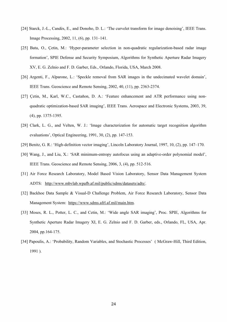
First we show an important capability of this method that is superresolution, which means that it can

reconstruct image details under bandwidth limitations. To demonstrate this property, we apply our method on

a synthetic scene composed of eight point scatterers with unit reflectivity magnitude and random (uniform)

uncorrelated phase. The magnitude field for this scene is shown in Fig. 1 (a). We set our system parameters so

that the system resolution is twice the image pixel size, so we seek superresolution reconstructions. Fig. 1 (b)

shows conventional spotlight mode SAR reconstruction using the polar format algorithm (PFA) [1] that

cannot resolve closely-spaced scatterers and suffers from high sidelobes. Fig. 1(c) shows the result of

nonquadratic regularization reconstruction method [2] by using regularizers for both point and region feature

enhancement. Note that this method also has superresolution capability when we just use the point

enhancement regularizer. However, as we usually do not have enough prior knowledge about the scene, here

16

we consider the scene may contain both point and region-based features. As it is seen, this technique fails to

reconstruct the scene accurately.

Fig. 1(d) shows the result of the proposed sparse representation method in which we observe that the

reconstructed image is very close to the true image. To be comparable with the result of nonquadratic

regularization method, here we have exploited an overcomplete shape-based dictionary which consists of

points as well as squares of various sizes at every possible location in the scene. Note that such a dictionary

can be used to sparsely represent many scenes containing point-like targets as well as smooth regions.

Experiment 2:

To demonstrate the capabilities of the proposed framework and contrast it with existing methods, in this

experiment we consider a more general synthetic scene composed of point scatterers as well as a smooth

distributed region as shown in Fig. 2(a). The image consists of 32×32 complex-valued pixels, and we show

only the magnitude field in Fig. 2(a). Phase is randomly distributed with a uniform density function in [-π,π].

The conventional image reconstruction based on PFA is shown in Fig. 2(b) which is a poor result. Fig. 2(c)

shows the nonquadratic regularization method with regularizers for both point and region enhancement. Note

that this method cannot enhance both types of features simultaneously in the reconstructed image due to

applying two contrary regularizers on the whole image. Whether the points or the regions are better preserved

is a trade off that could be adjusted through the regularization parameters.

Fig. 2(d) through Fig. 2(f) show the reconstructed images with the proposed sparse representation method

using dictionaries described in subsections 2.5.1 and 2.5.2. The shape-based (SB) dictionary here, which

consists of points as well as squares of various sizes at every possible location of the scene, has a good sparse

representation for the magnitude of this synthetic image, so the reconstructed image with this dictionary in

Fig. 2(d) is very close to the perfect reconstruction. Note that for better comparison of all results, we have not

shown the values below 50 dB of the maximum value of the image.

The multiresolution wavelet dictionary is a much more general dictionary that can be used for unknown

complicated scenes. Here we have used the Haar wavelet. Its result which is shown in Fig. 2(e) shows an

interesting and relatively good agreement with the true scene. As this figure shows, it seems that using

wavelet dictionary alone in the proposed framework is not so powerful to reconstruct the point scatterers. To

17

overcome this problem we propose to use an overcomplete dictionary composed of point dictionary (i.e.,

spikes) and the wavelet. The result obtained by using this overcomplete dictionary is shown in Fig. 2(f) where

it clearly represents both the smooth region and point targets. Consider that while the shape-based dictionary

appears to be very good in terms of reconstruction quality, computationally it is the most demanding one as it

is based on a highly redundant overcomplete dictionary. Evaluation results using quality metrics defined in

Section 3.2 are shown in Table 1 which demonstrate the superiority of the proposed SR-based methods.

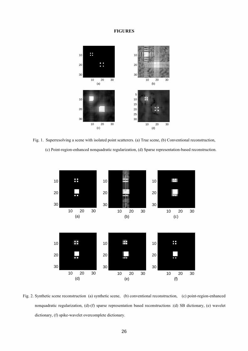
Experiment 3:

To be more realistic, in this experiment we use a synthetic image, constructed from the MIT Lincoln

Laboratory Advanced Detection Technology Sensor (ADTS) data set [31] by segmentation techniques, as

well as addition of some point scatterers (with random phase), as shown in Fig. 3(a). The conventional and

nonquadratic regularization reconstructions are shown in Fig. 3(b) and Fig. 3(c) respectively. Fig. 3(d)

through Fig. 3(f) show the reconstructed images with the sparse representation method with different

dictionaries. We have used the same shape-based dictionary described in the previous experiment. Because of

nonzero background and arbitrary distributed regions, the representation of this image is not as sparse as the

one in the previous synthetic scene, however the resultant reconstructed image still is in good agreement with

the true image. We can see in Fig. 3(f) that for this more realistic scene, the overcomplete spike-wavelet

dictionary has excellent result. We have used the Haar wavelet for this experiment. Evaluation results using

previously defined quality metrics are depicted in Table 1 which show the improvements achieved using the

proposed SR-based methods.

3.4 AFRL BACKHOE DATA

Experiment 4:

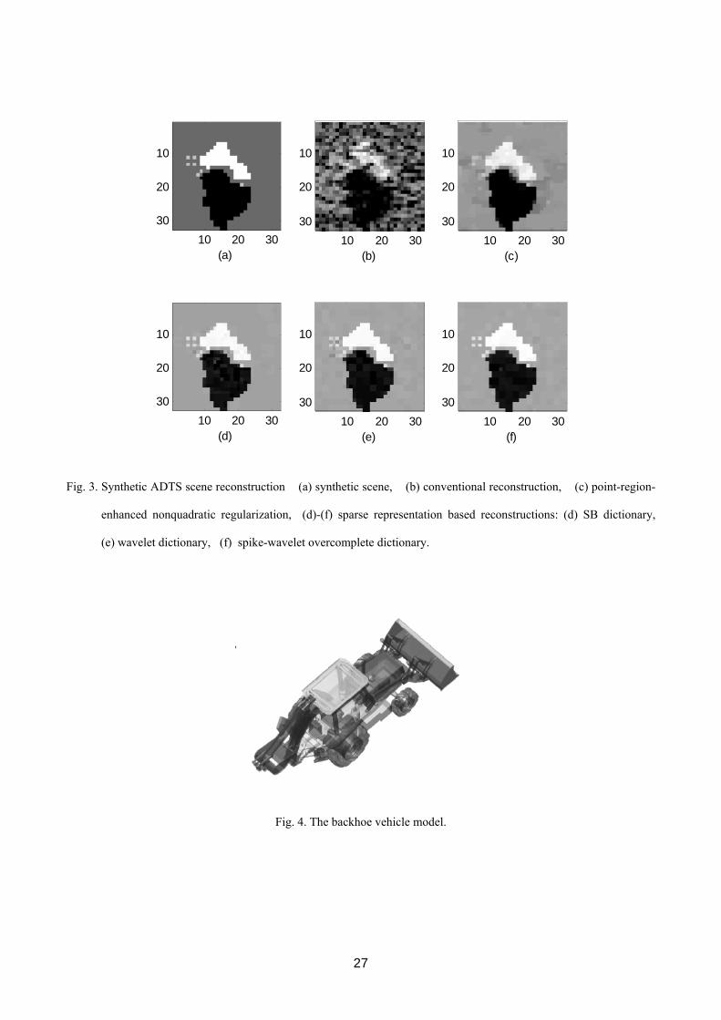
We now present our experimental results based on the AFRL Backhoe Data [32], which is a wideband, full

polarization, complex-valued backscattered data from a backhoe vehicle (shown in Fig. 4) in free space. In

our experiment we use VV polarization data centered at 10 GHz with three available bandwidths of 500 MHz,

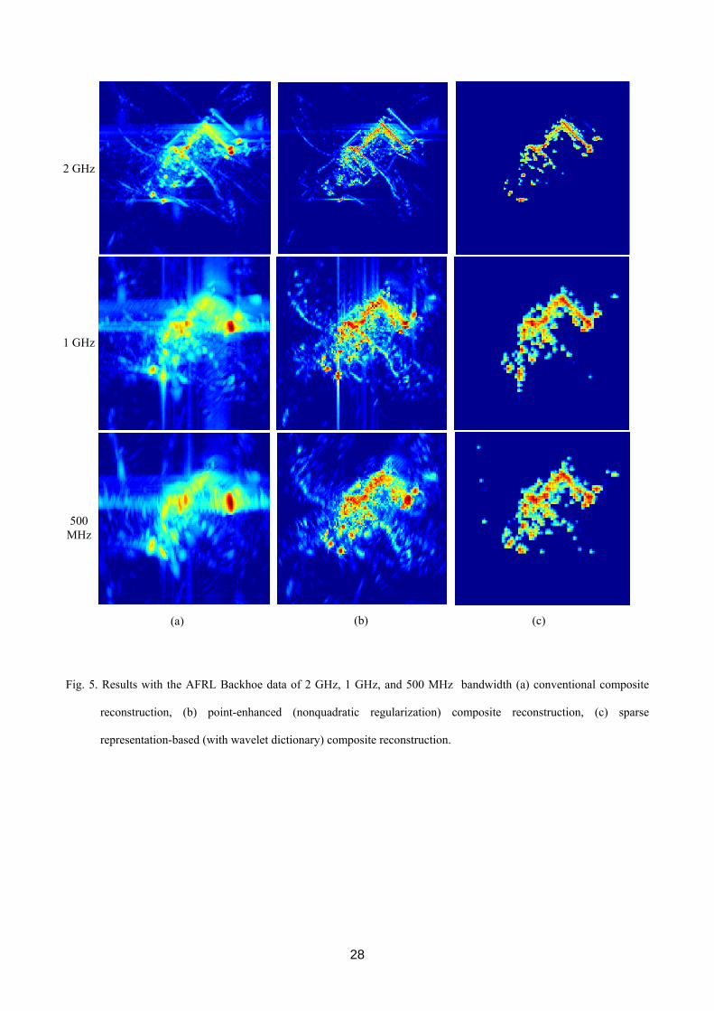
1 GHz, and 2 GHz, with an azimuthal span of 110° (centered at 45°). Fig. 5(a) shows the conventional

composite reconstructions of this data as described in [33] for bandwidths of 500 MHz, 1GHz, and 2GHz. We

obtain the composite images through combination of 19 subapertures, in each of which we use the spotlight-

18

mode SAR formulation. Also, a point-enhanced composite reconstruction method using nonquadratic

regularization has been recently presented in [5] for backhoe data. Fig. 5(b) shows the reconstructed images

based on this technique. Fig. 5(c) shows the results based on our proposed method using the wavelet

dictionary. We should expect to get the sparsest representation of the important/interested features (according

to the selected dictionary) in the reconstructed image. For better comparison, in all results of Fig. 5, the values

below 55dB of the image maximum value are not shown. As it is expected, for this complicated scene using

the wavelet dictionary, the sparse representation method produces very good results with very little artifacts.

Also based on our knowledge of the shape and structure of the scene there are very little false targets/features

out of the expected zone of the backhoe vehicle. We have used the Daubechies 2 (db2) wavelet for this

experiment. Quantitative evaluation results depicted in Tables 2 and 3 demonstrate the improved quality of

SR-based reconstructions in terms of all quality metrics except the MLW, for which the nonquadratic

regularization method is the best with the proposed SR-based method following close behind. Note that the

point-enhanced nonquadratic method is optimized for enhancing spike like targets and therefore it is expected

to have better MLW.

Experiment 5:

Finally in the last experiment we show the improved robustness of the sparse representation method in data

limitation scenarios. One important data limitation scenario that may occur in many SAR applications is

frequency band omission that may be encountered in several situations such as jamming and data dropouts or

in VHF/UHF frequency band systems such as foliage penetration (FOPEN) radar in which it is likely that we

will not be able to use an uninterrupted frequency band [5]. In this experiment for each of the three available

bandwidths of Backhoe data, we consider the case of frequency-band omissions where 20% of the spectral

data within that bandwidth are available. We have selected the available band randomly, with a preference for

contiguous bands (expressed through a parameter used in random band generation). The corresponding results

for this case are shown in Fig. 6. In these results the top 50 dB part of all images are shown for better

comparison. Robustness of the proposed sparse representation framework to bandwidth limitations as well as

frequency band data limitations is clearly revealed in these results. In Tables 2 and 3 computed quality

metrics are depicted which show the improvements provided by the proposed SR-based reconstructions in

19

terms of all quality metrics. It is interesting that here MLW of SR-based are better than that of nonquadratic

method which shows its excellent robustness to data limitation scenarios.

4. CONCLUSIONS

In this paper we have proposed a new approach for SAR image formation based on sparse signal

representation. Due to the complex-valued nature of the SAR reflectivities, we have designed our approach to

sparsely represent the magnitude of the complex-valued scattered field in terms of the features of interest. We

have formulated the mathematical framework for this method and proposed an iterative algorithm to solve the

corresponding joint optimization problem over the representation of magnitude and phase of the underlying

field reflectivities. In various experiments, we have demonstrated the performance of this approach which

produces high quality SAR images with enhanced features and very little artifacts, which is ideal for

automatic recognition tasks. Selection of the dictionary depends on the application. For SAR images of

natural scenes wavelet dictionary seems to be a good choice and for images of man-made targets with known-

shape parts, SB dictionaries could result in better reconstructions than the standard dictionaries at the expense

of higher computational load. Also as we have demonstrated, this approach exhibits interesting features

including superresolution, and robustness to bandwidth limitations as well as to uncertain and limited data.

Thus, it could be a good choice in such scenarios. In addition to these characteristics, the proposed approach

has the potential to provide enhanced image quality in non-conventional data collection scenarios, e.g. those

involving sparse apertures.

APPENDIX A

DERIVATION OF THE PDF OF β

Consider the complex random variable ijiiii ervju φ=+=)(β . Here, we know that ri=1 independent of φi,

and φi possesses a uniform pdf over |φi|<π which we denote it by U(φi). The pdf of the complex valued

random variable (β)i can be defined as [34]:

),(),(p

),(p))((pii

iiiii rJ

rvu

φφ

==β (A-1)

where the Jacobian J(ri,φi) = ri . Since ri and φi are independent:

20

)(U)1(δ)(p)(p),(p iiiiii rrr φφφ −== (A-2)

Thus, p((β)i) can be written as:

))((U)1|)((|δ)(U)1(δ)(U)1(δ1),(),(p

),(p))((p iiiiiiiii

iiiii rr

rrJr

vu βββ ∠−=−=−=== φφφφ

(A-3)

Since |(β)i| = 1 , ∀ i independent of each other and the phase terms, and also since all φi random variables are

assumed to be independent, Equation (12) follows.

APPENDIX B

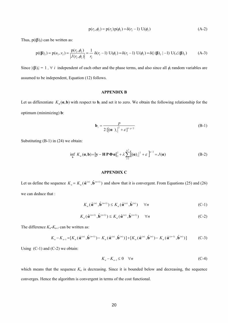
Let us differentiate ),(α bαK with respect to bi and set it to zero. We obtain the following relationship for the

optimum (minimizing) b:

2/12 ])([2 pi

ip

−+=

εαb (B-1)

Substituting (B-1) in (24) we obtain:

[ ] )()(),(inf2

1

2/222 αααΦPHybα

bJK

N

i

p

i =++−= ∑=

ελα (B-2)

APPENDIX C

Let us define the sequence )ˆ,ˆ( )1()( += nnn KK bαα and show that it is convergent. From Equations (25) and (26)

we can deduce that :

nKK nnnn ∀≤+ )ˆ,ˆ()ˆ,ˆ( )()()1()( bαbα αα (C-1)

nKK nnnn ∀≤ +++ )ˆ,ˆ()ˆ,ˆ( )1()()1()1( bαbα αα (C-2)

The difference Kn-Kn-1 can be written as:

])ˆ,ˆ()ˆ,ˆ([])ˆ,ˆ()ˆ,ˆ([ )()1()()()()()1()(1

nnnnnnnnnn KKKKKK bαbαbαbα −+− −+−=− αααα (C-3)

Using (C-1) and (C-2) we obtain:

nKK nn ∀≤− − 01 (C-4)

which means that the sequence Kn is decreasing. Since it is bounded below and decreasing, the sequence

converges. Hence the algorithm is convergent in terms of the cost functional.

21

APPENDIX D

We want to find s that minimizes ),( sββK of Equation (31). The portion of ),( sββK that depends on s is its

second term, as follows:

∑=

−2

1

21)(N

iiSβ (D-1)

[ ]{ }[ ]iiiiiii jj sββββsSβ −ℜ−+=−−=− )(exp()(21)(1)()exp(1)( 222 φ (D-2)

where [ ]i)(βφ denotes the phase of the complex number i)(β . The sum in (D-1) takes its minimum value when

the term inside the bracket in (D-2) has a zero imaginary part for all i. Therefore the s that minimizes the sum

in (D-1) and hence Equation (31) satisfies:

iii ∀= ])[(βs φ (D-3)

With this s, we have Sβ = |β|, and hence:

)()1)((),(inf2

1

222 βββBHysβ

sJK

N

ii =−′+−= ∑

=

λβ (D-4)

APPENDIX E

Considering that B=diag{Φα } and P=diag{β}, the cost functions of (8) and (14) both are actually functions

of α and β. Note that the first part ( 2l -norm data dependent term) of both cost functions are equal for given

α and β, so we denote the data term by J1(α ,β). Based on that, let us define a total cost function as below:

∑=

−′++=2

1

21 1))((),(),(

N

ii

ppt λJJ βαβαβα λ (E-1)

Note that finding the minimizing α for ),( βαtJ reduces to the optimization problem in (8), and finding the

minimizing β for ),( βαtJ reduces to the optimization problem in (14). Thus, the overall image reconstruction

algorithm of Section 2.2 is actually a block coordinate descent approach as follows:

)ˆ,(minargˆ )()1( lt

l J βααα

=+ (E-2)

),ˆ(minargˆ )1()1( βαββ

++ = lt

l J (E-3)

22

where l denotes the iteration number of the overall algorithm. Using Equations (E-2) and (E-3), convergence

of the overall algorithm in terms of cost functional can be easily established in a similar way to the one in

Appendix C.

REFERENCES

[1] Carrara, W. G., Goodman, R. S., and Majewski, R. M.: ‘Spotlight Synthetic Aperture Radar: Signal

Processing Algorithms’ (Artech House, Boston, MA, 1995).

[2] Çetin, M., and Karl, W.C.: ‘Feature-enhanced synthetic aperture radar image formation based on

nonquadratic regularization’, IEEE Trans. Image Processing, 2001, 10, (4), pp. 623–631.

[3] Munson Jr., D. C., O’Brien, J. D., and Jenkins, W. K.: ‘A tomographic formulation of spotlight-mode

synthetic aperture radar’, Proceedings of the IEEE, 1983, 71, pp. 917-925.

[4] Kak, A. C., and Slaney, M.: ‘Principles of Computerized Tomographic Imaging’ (IEEE Press, New York,

1988).

[5] Çetin, M., and Moses, R. L.: ‘SAR imaging from partial-aperture data with frequency-band omissions’,

SPIE Defense and Security Symposium, Algorithms for Synthetic Aperture Radar Imagery XII, E. G.

Zelnio and F. D. Garber, Eds., Orlando, Florida, USA, March 2005, pp. 32-43.

[6] Chen, S. S., Donoho, D. L., and Saunders, M. A.: ‘Atomic decomposition by basis pursuit’, SIAM J. Sci.

Comput., 1998, 20, pp. 33-61.

[7] Donoho, D. L., and Huo, X.: ‘Uncertainty principles and ideal atomic decomposition’, IEEE Trans. Inf.

Theory, 2001, 47, (7), pp. 2845–2862.

[8] Donoho, D. L., and Elad, M.: ‘Maximal sparsity representation via l1 minimization’, Proc. Nat. Acad. Sci.,

2003, 100, pp. 2197–2202.

[9] Elad, M., and Bruckstein, A.: ‘A generalized uncertainty principle and sparse representation in pairs of

bases’, IEEE Trans. Inf. Theory, 2002, 48, (9), pp. 2558–2567.

[10] Chartrand, R.: ‘Exact reconstruction of sparse signals via nonconvex minimization’, IEEE Signal

Processing Letters, 2007, 14, (10), pp. 707-710.

23

[11] Malioutov, D.M., Cetin, M., Willsky, A.S.: ‘Optimal sparse representations in general overcomplete

bases’, IEEE International Conference on Acoustics, Speech, and Signal Processing (ICASSP), May

2004, pp. 793-796.

[12] S. M. Kay: ‘Fundamentals of Statistical Signal Processing: Estimation Theory’ ( Prentice-Hall,

Englewood Cliffs, NJ, 1993).

[13] B. Borden: ‘Maximum entropy regularization in inverse synthetic aperture radar imagery’, IEEE Trans.

Signal Processing, 1992, 40, (4), pp. 969–973.

[14] Mensa, D. L.: ‘High Resolution Radar Imaging’ ( Artech House, Dedham, MA, 1981).

[15] Munson Jr., D. C., and Sanz, J. L. C.: ‘Image reconstruction from frequency-offset Fourier data’,

Proceedings of the IEEE, 1984, 72, pp. 661–669.

[16] Vogel, C. R., and Oman, M. E.: ‘Iterative methods for total variation denoising’, SIAM J. Sci. Comput.,

1996, 17, (1), pp. 227–238.

[17] Golub, G. H., and Van Loan, C. F.: ‘Matrix Computations’ ( The Johns Hopkins University Press,

Baltimore, MD, 1996).

[18] Çetin, M., Karl, W.C., and Willsky, A. S.: ‘Feature-preserving regularization method for complex-valued

inverse problems with application to coherent imaging’, Optical Engineering, 2006, 45, (1): 017003.

[19] Geman, D., and Yang, C.: ‘Nonlinear image recovery with half-quadratic regularization’, IEEE Trans.

Image Processing, 1995, 4, (7), pp. 932–946.

[20] Starck, J. L., Elad, M., and Donoho, D. L.: ‘Image decomposition via the combination of sparse

representations and a variational Approach’, IEEE Trans. Image Processing, 2005, 14, (10), pp. 1570-

1582.

[21] Donoho, D. L., and Johnstone, I.: ‘Ideal spatial adaptation via wavelet shrinkage’, Biometrika, 1994, 81,

pp. 425-455.

[22] Zeng, Z., and Cumming, I. G.: ‘SAR image data compression using a tree-structured wavelet transform’,

IEEE Trans. Geoscience and Remote Sensing, 2001, 39, (3), pp. 546-552.

[23] Rilling, G., Davies, M., and Mulgrew, B.: ‘Compressed sensing based compression of SAR raw data’,

Signal Processing with Adaptive Sparse Structured Representations Workshop, Saint-Malo, France,

April 2009.

24

[24] Starck, J.-L., Candès, E., and Donoho, D. L.: ‘The curvelet transform for image denoising’, IEEE Trans.

Image Processing, 2002, 11, (6), pp. 131–141.

[25] Batu, O., Çetin, M.: ‘Hyper-parameter selection in non-quadratic regularization-based radar image

formation’, SPIE Defense and Security Symposium, Algorithms for Synthetic Aperture Radar Imagery

XV, E. G. Zelnio and F. D. Garber, Eds., Orlando, Florida, USA, March 2008.

[26] Argenti, F., Alparone, L.: ‘Speckle removal from SAR images in the undecimated wavelet domain’,

IEEE Trans. Geoscience and Remote Sensing, 2002, 40, (11), pp. 2363-2374.

[27] Çetin, M., Karl, W.C., Castañon, D. A.: ‘Feature enhancement and ATR performance using non-

quadratic optimization-based SAR imaging’, IEEE Trans. Aerospace and Electronic Systems, 2003, 39,

(4), pp. 1375-1395.

[28] Clark, L. G., and Velten, W. J.: ‘Image characterization for automatic target recognition algorithm

evaluations’, Optical Engineering, 1991, 30, (2), pp. 147-153.

[29] Benitz, G. R.: ‘High-definition vector imaging’, Lincoln Laboratory Journal, 1997, 10, (2), pp. 147–170.

[30] Wang, J., and Liu, X.: ‘SAR minimum-entropy autofocus using an adaptive-order polynomial model’,

IEEE Trans. Geoscience and Remote Sensing, 2006, 3, (4), pp. 512-516.

[31] Air Force Research Laboratory, Model Based Vision Laboratory, Sensor Data Management System

ADTS: http://www.mbvlab.wpafb.af.mil/public/sdms/datasets/adts/.

[32] Backhoe Data Sample & Visual-D Challenge Problem, Air Force Research Laboratory, Sensor Data

Management System: https://www.sdms.afrl.af.mil/main.htm.

[33] Moses, R. L., Potter, L. C., and Cetin, M.: ‘Wide angle SAR imaging’, Proc. SPIE, Algorithms for

Synthetic Aperture Radar Imagery XI, E. G. Zelnio and F. D. Garber, eds., Orlando, FL, USA, Apr.

2004, pp.164-175.

[34] Papoulis, A.: ‘Probability, Random Variables, and Stochastic Processes’ ( McGraw-Hill, Third Edition,

1991 ).

25

LIST OF FIGURE CAPTIONS

Fig. 1. Superresolving a scene with isolated point scatterers. (a) True scene, (b) Conventional reconstruction,

(c) Point-region-enhanced nonquadratic regularization, (d) Sparse representation-based reconstruction.

Fig. 2. Synthetic scene reconstruction (a) synthetic scene, (b) conventional reconstruction, (c) point-region-enhanced

nonquadratic regularization, (d)-(f) sparse representation based reconstructions :(d) SB dictionary, (e) wavelet

dictionary, (f) spike-wavelet overcomplete dictionary.

Fig. 3. Synthetic ADTS scene reconstruction (a) synthetic scene, (b) conventional reconstruction, (c) point-region-

enhanced nonquadratic regularization, (d)-(f) sparse representation based reconstructions: (d) SB dictionary,

(e) wavelet dictionary, (f) spike-wavelet overcomplete dictionary.

Fig. 4. The backhoe vehicle model.

Fig. 5. Results with the AFRL Backhoe data of 500 MHz, 1 GHz, and 2 GHz bandwidth (a) conventional composite

reconstruction, (b) point-enhanced (nonquadratic regularization) composite reconstruction, (c) sparse

representation-based (with wavelet dictionary) composite reconstruction.

Fig. 6. Results with the AFRL Backhoe data of 500 MHz, 1 GHz, and 2 GHz bandwidth with frequency band omissions

(20% of the full band data available) (a) conventional composite reconstruction, (b) point-enhanced (nonquadratic

regularization) composite reconstruction, (c) sparse representation-based (with wavelet dictionary) composite

reconstruction.

26

FIGURES

(a)10 20 30

10

20

30

(b)10 20 30

10

20

30

(c)10 20 30

10

20

30

(d)10 20 30

5

10

15

20

25

30

Fig. 1. Superresolving a scene with isolated point scatterers. (a) True scene, (b) Conventional reconstruction,

(c) Point-region-enhanced nonquadratic regularization, (d) Sparse representation-based reconstruction.

(a)10 20 30

10

20

30

(b)10 20 30

10

20

30

(c)10 20 30

10

20

30

(e)10 20 30

10

20

30

(d)10 20 30

10

20

30

(f)10 20 30

10

20

30

Fig. 2. Synthetic scene reconstruction (a) synthetic scene, (b) conventional reconstruction, (c) point-region-enhanced

nonquadratic regularization, (d)-(f) sparse representation based reconstructions :(d) SB dictionary, (e) wavelet

dictionary, (f) spike-wavelet overcomplete dictionary.

27

(a)10 20 30

10

20

30

(b)10 20 30

10

20

30

(c)10 20 30

10

20

30

(e)10 20 30

10

20

30

(d)10 20 30

10

20

30

(f)10 20 30

10

20

30

Fig. 3. Synthetic ADTS scene reconstruction (a) synthetic scene, (b) conventional reconstruction, (c) point-region-

enhanced nonquadratic regularization, (d)-(f) sparse representation based reconstructions: (d) SB dictionary,

(e) wavelet dictionary, (f) spike-wavelet overcomplete dictionary.

Fig. 4. The backhoe vehicle model.

28

Fig. 5. Results with the AFRL Backhoe data of 2 GHz, 1 GHz, and 500 MHz bandwidth (a) conventional composite

reconstruction, (b) point-enhanced (nonquadratic regularization) composite reconstruction, (c) sparse

representation-based (with wavelet dictionary) composite reconstruction.

(a) (b) (c)

500 MHz

1 GHz

2 GHz

29

Fig. 6. Results with the AFRL Backhoe data of 2 GHz, 1 GHz, and 500 MHz bandwidth with frequency band omissions

(20% of the full band data available) (a) conventional composite reconstruction, (b) point-enhanced (nonquadratic

regularization) composite reconstruction, (c) sparse representation-based (with wavelet dictionary) composite

reconstruction.

(a) (b) (c)

500 MHz

1 GHz

2 GHz

30

Table1 Evaluation results of experiments2 and 3 Conventional Nonquadratic SR-SB SR-wavelet SR-spkwav

SNR(dB) 11.50 16.22 27.76 22.07 27.95 Experiment 2 TLM(%) 85.25 92.57 98.14 96.87 99.70

SNR(dB) 13.87 23.01 29.72 28.31 30.03 Experiment 3 TLM(%) 78.22 98.82 99.80 99.31 100

Table 2 Evaluation results of experiments 4 and 5 ( true scene-dependent metrics) 1GHz 500MHz

Conventional Nonquadratic SR-wav Conventional Nonquadratic SR-wav SNR(dB) 28.01 28.65 31.33 28.19 28.55 30.87 Experiment

4 TLM(%) 80.71 85.11 91.02 80.88 85.89 91.01 SNR(dB) 26.27 27.39 30.34 26.03 26.50 29.87 Experiment

5 TLM(%) 77.76 86.36 89.24 77.60 84.90 89.85

Table 3 Evaluation results of experiments 4 and 5 (unknown scene metrics) 2GHz 1GHz 500MHz

Conv. Nonq. SR-wav Conv. Nonq. SR-wav Conv. Nonq. SR-wav TBR(dB) 50.01 55.31 71.99 43.07 47.42 60.47 42.47 47.86 58.42 MLW(m) 0.061 0.016 0.019 0.141 0.034 0.040 0.293 0.074 0.082 ENT 1.485 1.003 0.475 2.324 1.789 1.026 2.138 1.865 1.140

Exper-iment

4 TBED 1.633 2.546 3.890 0.930 1.735 3.362 0.973 1.779 3.230 TBR(dB) 36.48 45.88 60.04 29.49 40.88 55.87 27.66 33.36 51.55 MLW(m) 0.099 0.028 0.020 0.185 0.040 0.040 0.456 0.091 0.084 ENT 3.250 2.118 0.804 4.048 2.690 1.271 4.403 3.657 1.323

Exper-iment

5 TBED 0.576 1.396 3.445 0.337 1.244 2.979 0.287 0.814 2.877