Sparse margin–based discriminant analysis for feature extraction

REVIEW

Sparse margin–based discriminant analysis for feature extraction

Zhenghong Gu • Jian Yang

Received: 29 October 2011 / Accepted: 30 July 2012

� Springer-Verlag London Limited 2013

Abstract The existing margin-based discriminant analy-

sis methods such as nonparametric discriminant analysis

use K-nearest neighbor (K-NN) technique to characterize

the margin. The manifold learning–based methods use

K-NN technique to characterize the local structure. These

methods encounter a common problem, that is, the nearest

neighbor parameter K should be chosen in advance. How to

choose an optimal K is a theoretically difficult problem. In

this paper, we present a new margin characterization

method named sparse margin–based discriminant analysis

(SMDA) using the sparse representation. SMDA can

successfully avoid the difficulty of parameter selection.

Sparse representation can be considered as a generalization

of K-NN technique. For a test sample, it can adaptively

select the training samples that give the most compact

representation. We characterize the margin by sparse

representation. The proposed method is evaluated by using

AR, Extended Yale B database, and the CENPARMI

handwritten numeral database. Experimental results show

the effectiveness of the proposed method; its performance

is better than some other state-of-the-art feature extraction

methods.

Keywords Sparse margin � Dimensional reduction �Feature extraction

1 Introduction

The curse of dimensionality [1] is a significant difficulty in

pattern recognition and computer vision. Dimensionality

reduction is an effective way to avoid this problem and

improving the computational efficiency. Researchers have

developed many algorithms for dimensional algorithms.

Among the linear algorithms, PCA [2, 3] and LDA [4] are

the two well-known methods and become the most popular

techniques in face recognition [2, 5]. LDA aims to find the

optimal projection such that the Fisher criterion (i.e., the

ratio of the between-class scatter to the within-class scatter)

is maximized after the projection of samples. LDA is

optimal in Bayes sense in the case that all classes share the

normal distribution with the same covariance matrix and

different means that cannot always be satisfied in read-

world applications. To overcome this problem, Fukunaga

et al. [6] presented a method named nonparametric dis-

criminant analysis (NDA). The method is a classic margin–

based discriminant analysis. The basis of extension of NDA

is a nonparametric between-class scatter matrix. It measures

between-class scatter based on marginal information, using

K-nearest neighbor (K-NN) technique. Li et al. [7, 8]

extended NDA to multi-class cases and developed a method

NSA. Li et al. [7, 8] further improved NSA by introducing a

nonparametric within-class scatter matrix. Qiu and Wu [9]

proposed a nonparametric margin maximum criterion

(NMMC) method. All of these nonparametric methods

characterize the margin by K-NN technique.

Linear models may fail to find the essential data structures

that are nonlinear. The maximal recognition rate of each

method and the corresponding dimension are listed in Table 1.

Manifold learning–based methods are developed to address

this problem. The purpose of manifold learning is to directly

find the intrinsic low-dimensional nonlinear data structures.

Z. Gu (&) � J. Yang

School of Computer Science and Technology,

Nanjing University of Science and Technology of China,

Nanjing 210094, People’s Republic of China

e-mail: [email protected]; [email protected]

J. Yang

e-mail: [email protected]

123

Neural Comput & Applic

DOI 10.1007/s00521-012-1124-x

Among the well-known are LPP [11], NPE [12], ISOMAP

[10], LLE [13], and Laplacian Eigenmap [14]. Recently,

Yan et al. [15] proposed a general dimensionality reduction

framework called graph embedding and developed a new

method MFA. LLE, ISOMAP, and Laplacian Eigenmap can

all be reformulated as a unified model in this framework.

These manifold methods such as MFA, LLE, and NPE

characterize the local structures by K-NN technique.

Both nonparametric methods and manifold-learning

methods encounter a problem that the neighborhood

parameter K should be chosen in advance. How to choose an

optimal K is a theoretically difficult problem. In this paper,

we present a new margin characterization method by virtue

of sparse representation. For a signal, sparse representation

searches its most compact representation in an overcomplete

dictionary. The signal will be represented as a compact

combination of a small number of atoms in the dictionaries.

In other words, the theory of sparse representation reveals

that sparse is the essential attribute of signals [16–20].

Wright et al. [21] exploit the discriminative nature of sparse

representation for classification and develop a classifier

based on sparse representation called SRC. Motived by this,

Zhang et al. [22] provided a dictionary method for face

recognition by discriminative K-SVD and sparse represen-

tation. Calderbank et al. [23] provided a compressed

learning method for sparse dimensionality reduction. SRC is

a linear method. Gao et al. [24] provided a Kernel sparse

representation for face recognition. Qiao et al. [25] provided

a dimensional reduction method called sparsity-preserving

projection (SPP) that constructs the weight matrix of the

data set based on a modified sparse representation frame-

work. In this paper, we propose a new discriminant analysis

method named sparse margin–based discriminant analysis

(SMDA). We construct the scatter matrix based on marginal

information that is characterized by sparse representation

instead of K-NN technique, so we call this margin as sparse

margin. The present method SMDA can successfully avoid

the difficulty of parameter selection. The proposed method

is applied to feature extraction.

The remainder of this paper is organized as follows: Sect. 2

gives a review of NDA and SPP. Section 3 describes our

method SMDA. Experimental evaluation of the proposed

method using the AR database, the Extended Yale B data-

base, and CENPARMI handwritten numeral database are

presented in Sect. 4. Finally, we give our conclusion in Sect. 5.

2 Related work

2.1 Nonparametric discriminant analysis

NDA is a classic margin–based discriminant analysis

method. The basis of extension of NDA is a nonparametric

between-class scatter matrix. It measures between-class

scatter based on marginal information, using K-NN tech-

nique. We denote the samples of class C1 and C2 as x and y,

respectively.

SNDAb ¼

XN1

i¼1

wiðxi � miÞðxi � miÞT

þXN2

j¼1

wjðyj � mjÞðyj � mjÞT ð1Þ

where N1 and N2 are the number of sample of C1 and C2,

respectively. mi ¼PK

l¼1 yil, mj ¼PK

l¼1 xjl, where yil is the

l-th nearest neighbor (NN) from C2 to xi, xjl is the l-th NN

from class 1 to yj, and wi is a weighting function to

deemphasize the samples far from the classification mar-

gin. NDA, however, encounters the problem of how to

choose the optimal K.

2.2 Sparsity preserving projection

The manifold method NPE aims to preserve the local

neighborhood structure of the data. NPE uses the affinity

weighting matrix using local least squares approximation.

The locality is characterized by K-NN technique. Instead of

K-NN technique, SPP constructed affinity weight matrix of

the data based on a modified sparse representation frame-

work. Given a set of training samples fxigni¼1, let D =

[x1, x2, …, xn][Rm9n be the dictionary matrix constructed

by all the training samples. SPP seeks a sparse recon-

structive weight vector Si for each xi through the modified

l1 minimization problem:

Min sik k1 s:t: xi ¼ Dsi; 1 ¼ 1T si ð2Þ

where si = [si1, …, si,i?1, 0, si1, …, sin]T. Then, the sparse

reconstructive weight matrix is S = [s1, s2, …, sn]T. SPP

uses the matrix S to reflect the intrinsic geometric

properties of the data. Similar to NPE, it seeks the

projections that best preserve the optimal weight vector si

by the following function

arg minW

WT DDT W¼1

Xn

i¼1

WT xi �WT Dsi

�� 2 ð3Þ

3 Sparse margin–based discriminant analysis

We use sparse representation to design a new discriminant

analysis method SMDA. SPP uses the sparse representation

Table 1 The maximal recognition rates (%) of PCA, LDA, LPP,

NDA, SPP, and SMDA and the corresponding dimensions on the

CENPARMI handwritten numeral database

PCA LDA LPP NDA SPP SMDA

87.0 88.4 89.2 88.4 85.8 92.5

29 9 30 19 30 25


123

to design the reconstructive weight matrix. SMDA uses

sparse representation to characterize between-class and

within-class scatters. This section introduces the basic idea

of SMDA, then formulates the algorithm for two-class

cases, and extends it to multi-class cases.

3.1 SMDA for two-class cases

The nonparametric between-class scatter matrix of NDA

involves a clustering procedure by the K-NN technique.

Sparse representation is used to replace K-NN technique in

our method. It can be referred to as a generalization of the

clustering problem [26].

Given two pattern classes C1 and C1, the training sam-

ples are x1,l, (l = 1, 2, …, N1) and x2,l, (l = 1, 2, …, N2),

respectively.

Let’s consider the one-side case first and begin with the

samples in C1. For a given sample x1,i [ C1, we denote

A ¼ ½x1;1; . . .x1;i�1;x1;iþ1; . . .; x1;N1� and B ¼ ½x2;1; . . .; x2;N2

�.Then, the overcomplete dictionary for x1,i is D = [A, B].

We seek a reconstructive vector by

a_

1;i ¼ arg min a1;i

�� 0

Subject to x1;i ¼ Da1;i ð4Þ

It is an NP-hard problem, but if the solution is sparse

enough, the solution of (4) is equivalent to the following

L1-minimization problem [27]:

a_

1;i ¼ arg min a1;i

�� 1

Subject to x1;i ¼ Da1;i ð5Þ

This problem can be solved by standard convex

programming method [28]. Our implementation is based

on sparselab [29]. Let’s change the form of the

representation as follows

x1;i ¼ Da1;i ¼ ½A;B�aA

1;i

aB1;i

� �¼ AaA

1;i þ BaB1;i ð6Þ

x1,i is decomposed into two parts, that is, the within-class

part AaA1;i and the between-class part BaB

1;i, following the

parallelogram rule, as illustrated by Fig. 1.

In NDA, margin samples are searched by K-NN tech-

nique, and the parameter K is nonadaptive. In our method,

margin samples are the support training samples of Class

C2, that is, the samples of Class C2 corresponding to non-

zero components of aB1;i. The number of margin samples

obtained by sparse representation is self-adaptive. On the

other hand, the importance of margin samples is different

for classification. Sparse representation computes the

weighting values of the margin samples, that is, aB1;i.

The individual between-class difference defined as

Db1;i ¼ x1;i � BaB

1;i ¼ AaA1;i ð7Þ

As illustrated by Fig. 1, the local sparse margin for sample

x1,i can be measured by L2-norm of Db1;i. The between-class

scatter matrix with respect to C1 is defined as

S1;b ¼XN1

i¼1

Db1;iðD

b1;iÞ

T ð8Þ

NDA uses a complicated weighting function to

deemphasize the samples far from the classification

margin, which exert negative influence for classification.

Our method does not need the weighting function, since the

farther away x1,i is from the classification margin, the less

the information BaB1;i contains. As a result, the weighting

function is unnecessary in our method SMDA.

The within-class scatter of x1,i is measured by within-

class difference Dw1;i.

Dw1;i ¼ x1;i � AaA

1;i ¼ BaB1;i ð9Þ

Then, we can also give a nonparametric version of within-

class scatter matrix Sw constructed by Dw1;i. Note that NDA

only suggests a nonparametric version of between-class

scatter matrix Sb.

The within-class scatter matrix with respect to Class C1

is defined as

S1;w ¼XN1

i¼1

Dw1;iðD

w1;iÞ

T ð10Þ

For the two-class cases, the between-class and within-class

scatter matrices are defined as

Sb ¼ S1;b þ S2;b ð11Þ

Sw ¼ S1;w þ S2;w ð12Þ

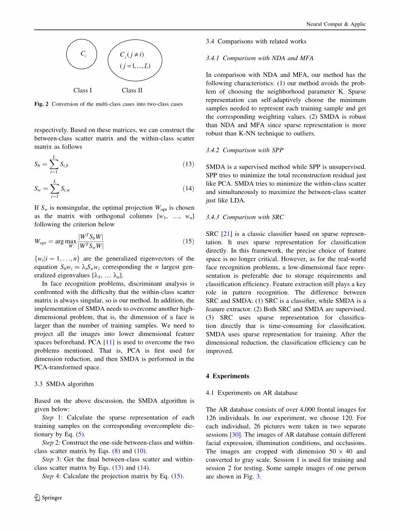
3.2 Extensions to multi-class cases

It is not hard to extend the SMDA algorithm to multi-class

cases. Suppose there are L pattern classes C1, …, CL. Let us

convert the multi-class cases into two-class cases in the

following way: Ci is viewed as one class and the remaining

is viewed as the other class, as illustrated by Fig. 2.

The between-class scatter matrix Si,b and within-class

scatter matrix Si,w can computed by (8) and (10),

1,ix

1,AiAα

1,BiBα1,

wiΔ

1,b

iΔ

1C 2C

Fig. 1 Illustration of SMDA for two-class cases. Here, O is the base

point. AaA1;i and BaB

1;i form the side a parallelogram. Db1;i is the local

sparse margin of x1,i. Dw1;i measures the within-class scatter of x1,i


123

respectively. Based on these matrices, we can construct the

between-class scatter matrix and the within-class scatter

matrix as follows

Sb ¼XL

i¼1

Si;b ð13Þ

Sw ¼XL

i¼1

Si;w ð14Þ

If Sw is nonsingular, the optimal projection Wopt is chosen

as the matrix with orthogonal columns [w1, …, wn]

following the criterion below

Wopt ¼ arg maxW

WT SbWj jWTSwWj j ð15Þ

wiji ¼ 1; . . .; nf g are the generalized eigenvectors of the

equation Sbwi = kiSwwi corresponding the n largest gen-

eralized eigenvalues [k1, … kn].

In face recognition problems, discriminant analysis is

confronted with the difficulty that the within-class scatter

matrix is always singular, so is our method. In addition, the

implementation of SMDA needs to overcome another high-

dimensional problem, that is, the dimension of a face is

larger than the number of training samples. We need to

project all the images into lower dimensional feature

spaces beforehand. PCA [11] is used to overcome the two

problems mentioned. That is, PCA is first used for

dimension reduction, and then SMDA is performed in the

PCA-transformed space.

3.3 SMDA algorithm

Based on the above discussion, the SMDA algorithm is

given below:

Step 1: Calculate the sparse representation of each

training samples on the corresponding overcomplete dic-

tionary by Eq. (5).

Step 2: Construct the one-side between-class and within-

class scatter matrix by Eqs. (8) and (10).

Step 3: Get the final between-class scatter and within-

class scatter matrix by Eqs. (13) and (14).

Step 4: Calculate the projection matrix by Eq. (15).

3.4 Comparisons with related works

3.4.1 Comparison with NDA and MFA

In comparison with NDA and MFA, our method has the

following characteristics: (1) our method avoids the prob-

lem of choosing the neighborhood parameter K. Sparse

representation can self-adaptively choose the minimum

samples needed to represent each training sample and get

the corresponding weighting values. (2) SMDA is robust

than NDA and MFA since sparse representation is more

robust than K-NN technique to outliers.

3.4.2 Comparison with SPP

SMDA is a supervised method while SPP is unsupervised.

SPP tries to minimize the total reconstruction residual just

like PCA. SMDA tries to minimize the within-class scatter

and simultaneously to maximize the between-class scatter

just like LDA.

3.4.3 Comparison with SRC

SRC [21] is a classic classifier based on sparse represen-

tation. It uses sparse representation for classification

directly. In this framework, the precise choice of feature

space is no longer critical. However, as for the real-world

face recognition problems, a low-dimensional face repre-

sentation is preferable due to storage requirements and

classification efficiency. Feature extraction still plays a key

role in pattern recognition. The difference between

SRC and SMDA: (1) SRC is a classifier, while SMDA is a

feature extractor. (2) Both SRC and SMDA are supervised.

(3) SRC uses sparse representation for classifica-

tion directly that is time-consuming for classification.

SMDA uses sparse representation for training. After the

dimensional reduction, the classification efficiency can be

improved.

4 Experiments

4.1 Experiments on AR database

The AR database consists of over 4,000 frontal images for

126 individuals. In our experiment, we choose 120. For

each individual, 26 pictures were taken in two separate

sessions [30]. The images of AR database contain different

facial expression, illumination conditions, and occlusions.

The images are cropped with dimension 50 9 40 and

converted to gray scale. Session 1 is used for training and

session 2 for testing. Some sample images of one person

are shown in Fig. 3.

Class I Class II

iC ( )

( 1,..., )jC j i

j L

≠

=

Fig. 2 Conversion of the multi-class cases into two-class cases


123

Our method is compared with Eigenface [2], Fisheface

[5], Laplacianface [31], nonparametric discriminant anal-

ysis (NDA) [6], and SPP [25]. All of these methods

including our method are used for feature extraction. In the

PCA phase of Fisherface, Laplacianface, NDA, SPP and

SMDA, we select the number of principal components as

180. After feature extraction, the nearest neighbor classifier

with cosine distance is employed for classification. The

recognition rate over the variation of dimensions is plotted

in Fig. 4. The maximal recognition rates of each method

and the corresponding dimension are listed in Table 2.

Figure 4 indicates that SMDA consistently performs better

than other methods when the dimension is over 40.

4.2 Experiment using the extended Yale B database

The Yale B face database [32] contains 5,760 single light

source images of 10 subjects each seen under 576 viewing

conditions (9 poses 9 64 illumination conditions). It was

updated to the Extended Yale B database [33] that contains

38 human subjects under 9 poses and 64 illumination

conditions. All test image data used in the experiments are

manually aligned, cropped, and then re-sized to 168 9 192

images [33].

All test images are under pose 00. Some sample images

of one person are shown in Fig. 5. In our experiment, we

resize each image to 42 9 48 pixels and further pre-pro-

cess it using histogram equalization. In our test, we use the

first 16 images per subject for training, the remaining 48

images for testing.

Fig. 3 Sample images of a person. The first row is from Session 1; the second row is from Session 2

10 20 30 40 50 60 70 80 90 100 110 1200

0.1

0.2

0.3

0.4

0.5

0.6

0.7

0.8

Dimension

Rec

ogni

tion

rate

Eigenface

Fisherface

LaplacianfaceNDA

SPP

SMDA

Fig. 4 Recognition rates of Eigenface, Fisherface, Laplacianface,

NDA, SPP, and SMDA on AR database

Fig. 5 Samples of a person under pose 00 and different illuminations,

which are cropped images in the extended Yale B face database

Table 2 The maximal recognition rates (%) of Eigenface, Fisherface,

Laplacianface, NDA, and SMDA and the corresponding dimensions

on the AR database

Eigenface Fisherface Laplacianface NDA SPP SMDA

61.8 66.9 57.4 67.1 68.6 72.3

120 110 120 110 120 120


123

In the PCA phase of Fisherface, Laplacianface, NDA,

SPP, and SMDA, we select the number of principal com-

ponents as 150. After feature extraction, we also use NN

classifier with cosine distance for classification. Figure 6

shows the recognition rate curve versus the variation of

dimensions. The maximal recognition rate of each method

and the corresponding dimension are listed in Table 3.

SMDA can outperform all the other methods when the

dimension is over 40. It seems that our method SMDA is

robust to variation of illumination.

4.3 Experiment using the CENPARMI handwritten

numeral database

The experiment was done on Concordia University

CENPARMI handwritten numeral database. The database

contains 6,000 samples of 10 numeral classes (each class

has 600 samples). In our experiment, we choose the first

200 samples of each class for training, the remaining 400

samples for testing. Thus, the total number of training

samples is 2,000 while the total number of testing samples

is 4,000.

PCA, LDA, LPP, NDA, SPP, and the proposed SMDA

are used, respectively, used for feature extraction based on

the original 121-dimensional Legendre moment features

[34]. The recognition rate curve of each method versus the

variation of dimensions is shown in Fig. 7.

5 Conclusion

We present a new linear feature extraction method called

sparse margin–based discriminant analysis (SMDA) in this

paper. The method characterizes the margin by sparse

representation. Based on this characterization, a class

margin criterion is designed for determining an optimal

transform matrix such that the sparse margin is maximal in

the transformed space. The proposed method was applied

to feature extraction and evaluated on the AR, the extended

Yale B database, and the CENPARMI handwritten numeral

database. The experimental results show that the proposed

method is more effective than Eigenface, Fisherface,

Laplacianface, NDA, and SPP methods.

Acknowledgments This work was partially supported by the

Program for New Century Excellent Talents in University of China,

the NUST Outstanding Scholar Supporting Program, the National

Science Foundation of China under Grants No. 60973098, 60632050

and 90820306.

References

1. Jain AK, Duin RPW, Mao J (2000) Statistical pattern recognition:

a review. IEEE Trans PAMI 22(1):4–37

2. Turk M, Pentland A (1991) Face recognition using eigenfaces. In:

IEEE conference on computer vision and pattern recognition.

Maui

3. Joliffe I (1986) Principal component analysis. Springer,

New York

4. Fisher RA (1936) The use of multiple measurements in taxo-

nomic problems. Ann Eugenics 7(2):179–188

20 40 60 80 100 1200.3

0.4

0.5

0.6

0.7

0.8

0.9

Dimension

Rec

ogni

tion

rate

Eigenface

Fisherface

LaplacianfaceNDA

SPP

SMDA

Fig. 6 Recognition rates of Eigenface, Fisherface, Laplacianface,

NDA, SPP, and SMDA on the Extended Yale B database

Table 3 The maximal recognition rates (%) of Eigenface, Fisherface,

Laplacianface, NDA, SPP, and SMDA and the corresponding

dimensions on the Extended Yale B database

Eigenface Fisherface Laplacianface NDA SPP SMDA

64.9 85.4 78.1 80.6 81.3 92.6

115 37 121 121 118 121

5 10 15 20 25 300

0.1

0.2

0.3

0.4

0.5

0.6

0.7

0.8

0.9

Dimension

Rec

ogni

tion

rate

PCA

LDA

LPPNDA

SPP

SMDA

Fig. 7 Recognition rates of PCA, LDA, LPP, NDA, SPP, and SMDA

versus the variation of dimensions on the CENPARMI handwritten

numeral database


123

5. Belhumeur P, Hespanha J, Kriegman D (1997) Eigenfaces versus

fisherfaces: recognition using class specific linear projection.

IEEE Trans Patt Anal Mach Intell 19(7):711–720

6. Fukunaga K, Mantock J (1983) Nonparametric discriminant

analysis. IEEE Trans Patt Anal Mach Intell 5:671C678

7. Li Z, Liu W, Lin D, Tang X (2005) Nonparametric subspace

analysis for face recognition. In: Proceedings of IEEE conference

on computer vision and pattern recognition

8. Li ZL, Lin DH, Tang XO (2009) Nonparametric discriminant

analysis for face recognition. IEEE Trans Patt Anal Mach Intell

31(4):2691–2698

9. Qiu XP, Wu LD (2005) Face recognition by stepwise nonpara-

metric margin maximum criterion. In: Proceedings of IEEE

conference on computer vision (ICCV 2005), Beijing

10. Tenenbaum JB, deSilva V, Langford JC (2000) A global geo-

metric framework for nonlinear dimensionality reduction. Sci-

ence 290:2319–2323

11. He X, Niyogi P (2002) Locality preserving projections (LPP).

TR-2002-09, 29 October

12. He X, Cai D, Yan S, Zhang H (2005) Neighborhood preserving

embedding. In: Proceedings in international conference on com-

puter vision (ICCV)

13. Roweis ST, Saul LK (2000) Nonlinear dimensionality reduction

by locally linear embedding. Science 290:2323–2326

14. Belkin M, Niyogi P (2003) Laplacian eigenmaps for dimen-

sionality reduction and data representation. Neural Comput

15(6):1373–1396

15. Yan S, Xu D, Zhang B, Zhang H-J (2005) Graph embedding: a

general framework for dimensionality reduction. In: Proceedings

of IEEE conference on computer vision and pattern recognition,

pp. 830–837

16. Mallat S, Zhang Z (1993) Matching pursuit in a time-frequency

dictionary. IEEE Trans Sig Process 41:3397–3415

17. Chen SS, Donoho DL, Saunders MA (1999) Atomic decompo-

sition by basis pursuit. SIAM J Sci Comput 20:33–61

18. Donoho DL, Huo X (2001) Uncertainty principles and ideal

atomic decomposition. IEEE Trans Inf Theor 47:2845–2862

19. Donoho DL (2006) Compressed sensing. IEEE Trans Inf Theor

52(4):1289–1306

20. Candes EJ, Wakin MB (2008) An introduction to compressive

sampling. IEEE Sig Process Mag 47:2845–2862

21. Wright J, Yang AY, Ganesh A, Sastry SS, Ma Y (2008) Robust

face recognition via sparse representation. Patt Anal Mach Intell

IEEE Trans 31(2):210–227

22. Zhang Q, Li B (2010) Discriminatie K-SVD for dictionary

learning in face recognition. IEEE, CVPR, pp 2691–2698

23. Calderbank R, Jafarpour S, Schapire R (2009) Compressed

learning: universal sparse dimensionality reduction and learning

in the measurement domain. Preprint

24. Gao S, Tsang I, Chia LT (2010) Kernel sparse representation for

image classification and face recognition, computer vision—

ECCV. Springer, Berlin, pp 1–14

25. Qiao L, et al (2009) Sparsity preserving projections with appli-

cation to face recognition. Patt Recogn 59:797–829

26. Aharon M, Elad M, Bruckstein AM (2006) The K-SVD: an

algorithm for designing of overcomplete dictionaries for sparse

representation. IEEE Trans Sig Process 54(11):4311–4322

27. Donoho D (2006) For most large underdetermined systems of

linear equations the minimal L1-norm solution is also the sparsest

solution. Comm Pure Appl Math 59(6):797–829

28. Chen S, Donoho D, Saunders M (2001) Atomic decomposition by

basis pursuit. SIAM Rev 43(1):129–159

29. Donoho D, Drori I, Stodden V, Tsaig Y (2005) Sparselab,

http://sparselab.stanford.edu/

30. Martinez A, Benavente R (1998) The AR face database. CVC

technical report 24

31. He X, Yan S, Hu Y, Niyogi P, Zhang H (2005) Face recognition

using laplacianfaces. IEEE Trans Patt Anal Mach Intell 27(3):

328–340

32. Georghiades AS, Belhumeur PN, Kriegman DJ (2001) From few

to many: illumination cone models for face recognition under

variable lighting and pose. IEEE Trans Patt Anal Mach Intell

23(6):643–660

33. Lee KC, Ho J, Driegman D (2005) Acquiring linear subspaces for

face recognition under variable lighting. IEEE Trans Patt Anal

Mach Intell 27(5):684–698

34. Liao SX, Pawlak M (1996) On image analysis by moments. IEEE

Trans Patt Anal Mach Intell 18(3):254–266


123

http://sparselab.stanford.edu/

Documents

Sparse margin–based discriminant analysis for feature extraction