Embed Size (px)
Citation preview

Sparse LA
Sathish Vadhiyar

Motivation Sparse computations much more
challenging than dense due to complex data structures and memory references
Many physical systems produce sparse matrices

Sparse Matrix-Vector Multiplication

Cache in GPUs Fermi has 16KB/48KB L1 cache per SM, and a global
768 KB L2 cache Each cache line is 128 bytes, to provide high
memory bandwidth Thus when using 48KB cache, only
(48KB/128bytes=384) cache lines can be stored GPUs execute up to 1536 threads per SM If all threads access different cache lines, 384 of
them will get cache hits, and others will get cache miss
Thus threads in the same block should work on the same cache lines

Compressed Sparse Row (CSR) Format
SpMV (Sparse Matrix-Vector Multiplication) using CSR

Naïve CUDA Implementation Assign one thread to each row Define block size as multiple of warp size, e.g.,
128 Can handle max of 128x65535=8388480 rows,
where 65535 is the max number of blocks

Naïve CUDA Implementation - Drawbacks
For large matrices with several elements per row, the implementation suffers from a high cache miss rate since cache can’t hold all cache lines being used
Thus coalescing/caching is poor for long rows
If nnz per row have high variance, warp divergence will occur

Thread Cooperation Multiple threads can be assigned to work on
the same row Cooperating threads act on adjacent elements
of the row; perform multiplication with elements of vector x; add up their results in shared memory using reduction
First thread of the group writes the result to vector y
If the number of cooperating threads, coop, is less than warp size, the synchronization between cooperating threads is implicit

Analysis
Same cache lines are used by cooperating threads
Improves coalescing/caching If the length of the row is not a
multiple of 32, can lead to warp divergence, and loss in performance
Coop = 4
Coalesced access; Good caching Warp divergence

Granularity If a group of cooperating threads act on only
row, then the number of blocks required for entire matrix may be more than 65535
Thus, more than one row per cooperating group can be processed
Number of rows processing by a cooperating group is denoted as repeat
A thread block processes repeat*blockSize/coop consecutive rows
An algorithm can be parametrized by blockSize, coop and repeat

Parametrized Algorithm

References
Efficient Sparse Matrix-Vector Multiplication on cache-based GPUs. Reguly, Giles. InPar 2012.
Tridiagonal Matrices

Parallel solution of linear system with special matricesTridiagonal Matrices
a1 h1
g2 a2 h2
g3 a3 h3
gn an
x1
x2
x3
.
.
xn
=
b1
b2
b3
.
.
bn
In general:
gixi-1 + aixi + hixi+1 = bi
Substituting for xi-1 and xi+1 in terms of {xi-2, xi} and {xi, xi+2} respectively:
Gixi-2 + Aixi + Hixi+2 = Bi

Tridiagonal Matrices
A1 H1
A2 H2
G3 A3 H3
G4 A4 H4
Gn-2 An
x1
x2
x3
.
.
xn
=
B1
B2
B3
.
.
Bn
Reordering:

Tridiagonal Matrices
A2 H2
G4 A4 H4
Gn An
A1 H1
G3 A3 H3
Gn-3 An-1
x2
x4
.
xn
x1
x3
.
xn-1
=
B2
B4
.
Bn
B1
B3
.
Bn-1

Tridiagonal Systems Thus the problem of size n has been split
into even and odd equations of size n/2 This is odd–even reduction For parallelization, each process can divide
the problem into subproblems of smaller size and solve the subproblems
This is divide-and-conquer technique

Tridiagonal Systems - Parallelization At each stage one representative process of the domain of
processes is chosen This representative performs the odd-even reduction of
problem i to two problems of size i/2 The problems are distributed to 2 representatives
1 2 3 4 5 6 7 8
1
2 6
1 3 5 7
n
n/2
n/4
n/8

Sparse Cholesky
To solve Ax = b; Most of the research and the base
case are in sparse symmetric positive definite matrices
A = LLT; Ly = b; LTx = y; Cholesky factorization introduces
fill-in

Column oriented left-looking Cholesky

Fill-in
10
13
2
4
5
6
7
8
9
10
13
2
4
5
6
7
8
9
Fill: new nonzeros in factor

Permutation Matrix or Ordering Thus ordering to reduce fill or to enhance
numerical stability Choose permutation matrix P so that
Cholesky factor L’ of PAPT has less fill than L.
Triangular solve:L’y = Pb; L’Tz = y; x = PTz The fill can be predicted in advance Static data structure can be used –
symbolic factorization
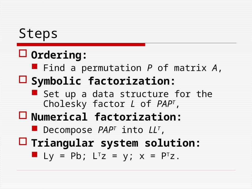
Steps Ordering:
Find a permutation P of matrix A, Symbolic factorization:
Set up a data structure for the Cholesky factor L of PAPT,
Numerical factorization: Decompose PAPT into LLT,
Triangular system solution: Ly = Pb; LTz = y; x = PTz.

Sparse Matrices and Graph Theory
1
2
3
4
5
6
7
1
2
3
4
5
6
7
1
2
3
4
5
6
7
2
3
4
5
6
7
1
2
3
4
5
6
7
1
2
3
4
5
6
7
3
4
5
6
7
4
5
6
7
G(A)

Sparse and Graph1
2
3
4
5
6
7
5
6
7
1
2
3
4
5
6
7
6
7
1
2
3
4
5
6
7
7
F(A)

Ordering
The above order of elimination is “natural”
The first heuristic is minimum degree ordering
Simple and effective But efficiency depends on tie
breaking strategy Difficult to parallelize!

Minimum degree ordering for the previous Matrix
1
2
3
4
5
6
7
Ordering – {2,4,5,7,3,1,6}
No fill-in !
6
1
5
2
3
7
4

Ordering Another ordering is nested dissection (divide-
and-conquer) Find separator S of nodes whose removal
(along with edges) divides the graph into 2 disjoint pieces
Variables in each pieces are numbered contiguously and variables in S are numbered last
Leads to bordered block diagonal non-zero pattern
Can be applied recursively Can be parallelized using divide-and-conquer
approach

Nested Dissection Illustration1
2
3
4
5
6
7
8
9
10
11
12
13
14
15
16
17
18
19
20
21
22
23
24
25
S

Nested Dissection Illustration1
3
5
7
9
2
4
6
8
10
21
22
23
24
25
11
13
15
17
19
12
14
16
18
20
S

Numerical Factorization
cmod(j, k): modification of column j by column k, k < j
cdiv(j) : division of column j by a scalar

Algorithms

Elimination Tree
T(A) has an edge between two vertices i and j, with i > j, if i = p(j), i.e., L(i, j) is first non-zero entry in the jth column below diagonal. i is the parent of j.
1
3
2
45
6
7
8
9
10

Parallelization of Sparse Cholesky
Most of the parallel algorithms are based on elimination trees
Work associated with two disjoint subtrees can proceed independently
Same steps associated with sequential sparse factorization
One additional step: assignment of tasks to processors

Ordering
2 issues: - ordering in parallel - find an ordering that will help in
parallelization in the subsequent steps

Ordering for Parallel Factorization
1
2
3
4
5
6
7
Natural order
1
2
3
4
5
6
7
Elimination Tree
No fill.
No scope for parallelization
No agreed objective for ordering for parallel factorization: Not all orderings that reduce fill-in can provide scope for parallelization

Example (Contd..)1
2
3
4
5
6
7
Nested dissection order
1
Elimination TreeFill.
But scope for parallelization
2
3
4 5
6
7
5
6
4
7
2
3
1

Ordering for parallel factorization – Tree restructuring
Decouple fill reducing ordering and ordering for parallel elimination
Determine a fill reducing ordering P of G(A)
Form the elimination tree T(PAPT) Transform this tree T(PAPT) to one with
smaller height and record the corresponding equivalent reordering, P’

Ordering for parallel factorization – Tree restructuring
Efficiency depends on if such an equivalent reordering can be found
Also on the limitations of the initial ordering, P
Only minor modifications to the initial ordering. Hence only limited improvement in parallelism
Algorithm by Liu (1989) based on elimination tree rotation to reduce the height
Algorithm by Jess and Kees (1982) based on chordal graph to reduce the height

Height and Parallel Completion time Not all elimination trees with minimum heights give
rise to small parallel completion times. Let each node, v, in elimination tree be associated
with x,y x – time[v] or time for factorization of column v y – level[v] level[v] = time[v] if v is the root of elimination tree,
time[v]+level[parent of v] otherwise Represents minimum time to completion starting at
node v Parallel completion time – maximum level value
among all nodes

Height and Parallel Completion time
a b c d e f g
h i
e
d
c
b
a
f
g
h
i
f
e
d
c
b
g
h
i
a1
2
3
4
5
6
7
8
9
1
2
3
4
5
6
7
8
9
2, 14
3, 12
3, 9
3, 6
4, 24
6, 20
6, 14
5, 8
3,3
2, 19
3, 17
3, 14
3, 11
3, 8
4, 21
6, 17
6, 11
5, 5

Minimization of Cost
Thus some algorithms (Weng-Yang Lin, J. of Supercomputing: 2003) pick at each step for ordering, the nodes with the minimum cost (greedy approach)

Ordering in Parallel – Nested dissection
Nested dissection can be carried in parallel Also leads to elimination trees that can be
parallelized during subsequent factorizations
But parallelization only in the later levels of dissection
Can be applied to only limited class of problems

Nested Dissection Algorithms
Use a graph partitioning heuristic to obtain a small edge separator of the graph
Transform the small edge separator into a small node separator
Number nodes of the separator last and recursively apply


K-L for ND Form a random initial partition Form edge separator by applying K-L
to form partitions P1 and P2 Let V1 in P1 such that nodes in V1
incident on atleast one edge in the separator set. Similarly V2
V1 U V2 (wide node separator), V1 or V2 (narrow node separator) by
Gilbert and Zmijewski (1987)

Step 2: Mapping Problems on to processors Based on elimination trees Various strategies to map columns to
processors based on elimination trees. Two algorithms:
Subtree-to-Subcube Bin-Pack by Geist and Ng

Naïve Strategy2
1
0
3
2
1
0 0
3 3
2 2
1 1
0 0 0 0
1 1
0 0 0 0

Strategy 2 – Subtree-to-subcube mapping
Select an appropriate set of P subtrees of the elimination tree, say T0, T1…
Assign columns corresponding to Ti to Pi Where two subtrees merge into a single
subtree, their processor sets are merged together and wrap-mapped onto the nodes/columns of the separator that begins at that point.
The root separator is wrap-mapped onto the set of all processors.

Strategy 20
1
2
3
0
1
0 2
1 3
0 2
0 1
0 0 1 1
2 3
2 2 3 3

Strategy 3: Bin-Pack (Geist and Ng) Subtree-to-subcube mapping is not good for unbalanced trees Try to find disjoint subtrees Map the subtrees to p bins based on first-fit-decreasing bin-
packing heuristic Subtrees are processed in decreasing order of workloads A subtree is packed into the current lightest bin
Weight imbalance, α – ratio between lightest and heaviest bin If α >= user-specified tolerance, γ, stop Else explore the heaviest subtree from the heaviest bin and
split into subtrees. These subtrees are then mapped to p bins and repacked using bin-packing again
Repeat until α >= γ or the largest subtree cannot be split further
Load balance based on user-specified tolerance For the remaining nodes from the roots of the subtrees to the
root of the tree, wrap map.

Parallel Numerical Factorization – Submatrix Cholesky
Tsub(k)
Tsub(k) is partitioned into various subtasks Tsub(k,1),…,Tsub(k,P) where
Tsub(k,p) := {cmod(j,k) | j C Struct(L*k) ∩ mycols(p)}

Definitions
mycols(p) – set of columns owned by p map[k] – processor containing column k procs(L*k) = {map[j] | j in Struct(L*k)}

Parallel Submatrix Choleskyfor j in mycols(p) do if j is a leaf node in T(A) do cdiv(j) send L*j to the processors in procs(L*j) mycols(p) := mycols(p) – {j}
while mycols(p) ≠ 0 do receive any column of L, say L*k
for j in Struct(L*k) ∩ mycols(p) do cmod(j, k) if column j required no more cmod’s do cdiv(j) send L*j to the processors in procs(L*j) mycols(p) := mycols(p) – {j}Disadvantages:
1. Communication is not localized

Parallel Numerical Factorization – Sub column Cholesky
Tcol(j) is partitioned into various subtasks Tcol(j,1),…,Tcol(j,P) where
Tcol(j,p) aggregates into a single update vector every update vector u(j,k) for which k C Struct(Lj*) ∩ mycols(p)

Definitions
mycols(p) – set of columns owned by p map[k] – processor containing column k procs(Lj*) = {map[k] | k in Struct(Lj*)} u(j, k) – scaled column accumulated into
the factor column by cmod(j, k)

Parallel Sub column Choleskyfor j:= 1 to n do if j in mycols(p) or Struct(Lj*) ∩ mycols(p) ≠ 0 do u = 0 for k in Struct(Lj*) ∩ mycols(p) do u = u + u(j,k) if map[j] ≠ p do send u to processor q = map[j] else incorporate u into the factor column j while any aggregated update column for column j remains unreceived do receive in u another aggregated update column for column j incoprporate u into the factor column j cdiv(j)
Has uniform and less communication than sub matrix version for subtree-subcube mapping

A refined version – compute-ahead fan-in
The previous version can lead to processor idling due to waiting for the aggregates for updating column j
Updating column j can be mixed with compute-ahead tasks:
1. Aggregate u(i, k) for i > j for each completed column k in Struct(Li*) ∩ mycols(p)
2. Receive aggregate update column for i > j and incorporate into factor column i

Sparse Iterative Methods

Iterative & Direct methods – Pros and Cons.
Iterative methods do not give accurate results.
Convergence cannot be predicted But absolutely no fills.

Parallel Jacobi, Gauss-Seidel, SOR
For problems with grid structure (1-D, 2-D etc.), Jacobi is easily parallelizable
Gauss-Seidel and SOR need recent values. Hence ordering of updates and sequencing among processors
But Gauss-Seidel and SOR can be parallelized using red-black ordering or checker board

2D Grid example
13
9
5
1
14
10
6
2
15
11
7
3
16
12
8
4

Red-Black Ordering
Color alternate nodes in each dimension red and black
Number red nodes first and then black nodes
Red nodes can be updated simultaneously followed by simultaneous black nodes updates

2D Grid example – Red Black Ordering
15
5
11
1
7
13
3
9
16
6
12
2
8
14
4
10
In general, reordering can affect convergence

Graph Coloring In general multi-colored graph coloring
Ordering for parallel computing of Gauss-Seidel and SOR
Graph coloring can also be used for parallelization of triangular solves
The minimum number of parallel steps in triangular solve is given by the chromatic number of symmetric graph
Unknowns corresponding to nodes of same color are solved in parallel; computation proceeds in steps
Thus permutation matrix, P based on graph color ordering

Parallel Triangular Solve based on Multi-Coloring Unknowns corresponding to the vertices of same color can
be solved in parallel Thus parallel triangular solve proceeds in steps equal to the
number of colors
1, 1
2, 73, 2
4, 3 6, 8
7, 9
5, 4
8, 59, 6
10, 10
Original Order New Order

Graph Coloring Problem Given G(A) = (V, E) σ: V {1,2,…,s} is s-coloring of G if
σ(i) ≠ σ(j) for every (i, j) edge in E Minimum possible value of s is
chromatic number of G Graph coloring problem is to color
nodes with chromatic number of colors
NP-complete problem

Parallel graph Coloring – General algorithm

Parallel Graph Coloring – Finding Maximal Independent Sets – Luby (1986)I = nullV’ = VG’ = GWhile G’ ≠ empty Choose an independent set I’ in G’ I = I U I’; X = I’ U N(I’) (N(I’) – adjacent vertices to I’) V’ = V’ \ X; G’ = G(V’)end
For choosing independent set I’: (Monte Carlo Heuristic)1. For each vertex, v in V’ determine a distinct random number p(v)2. v in I iff p(v) > p(w) for every w in adj(v)
Color each MIS a different color
Disadvantage: Each new choice of random numbers requires a global
synchronization of the processors.

Parallel Graph Coloring – Gebremedhin and Manne (2003)
Pseudo-Coloring

References in Graph Coloring M. Luby. A simple parallel algorithm for the maximal
independent set problem. SIAM Journal on Computing. 15(4)1036-1054 (1986)
M.T.Jones, P.E. Plassmann. A parallel graph coloring heuristic. SIAM journal of scientific computing, 14(3): 654-669, May 1993
L. V. Kale and B. H. Richards and T. D. Allen. Efficient Parallel Graph Coloring with Prioritization, Lecture Notes in Computer Science, vol 1068, August 1995, pp 190-208. Springer-Verlag.
A.H. Gebremedhin, F. Manne, Scalable parallel graph coloring algorithms, Concurrency: Practice and Experience 12 (2000) 1131-1146.
A.H. Gebremedhin , I.G. Lassous , J. Gustedt , J.A. Telle, Graph coloring on coarse grained multicomputers, Discrete Applied Mathematics, v.131 n.1, p.179-198, 6 September 2003

References M.T. Heath, E. Ng, B.W. Peyton. Parallel
Algorithms for Sparse Linear Systems. SIAM Review. Vol. 33, No. 3, pp. 420-460, September 1991.
A. George, J.W.H. Liu. The Evolution of the Minimum Degree Ordering Algorithm. SIAM Review. Vol. 31, No. 1, pp. 1-19, March 1989.
J. W. H. Liu. Reordering sparse matrices for parallel elimination. Parallel Computing 11 (1989) 73-91

References Anshul Gupta, Vipin Kumar. Parallel
algorithms for forward and back substitution in direct solution of sparse linear systems. Conference on High Performance Networking and Computing. Proceedings of the 1995 ACM/IEEE conference on Supercomputing (CDROM).
P. Raghavan. Efficient Parallel Triangular Solution Using Selective Inversion. Parallel Processing Letters, Vol. 8, No. 1, pp. 29-40, 1998

References
Joseph W. H. Liu. The Multifrontal Method for Sparse Matrix Factorization. SIAM Review. Vol. 34, No. 1, pp. 82-109, March 1992.
Gupta, Karypis and Kumar. Highly Scalable Parallel Algorithms for Sparse Matrix Factorization. TPDS. 1997.