Sparse estimation of a covariance matrix

Biometrika (2011), 98, 4, pp. 807–820 doi: 10.1093/biomet/asr054C© 2011 Biometrika Trust

Printed in Great Britain

Sparse estimation of a covariance matrix

BY JACOB BIEN AND ROBERT J. TIBSHIRANI

Departments of Statistics and Health, Research & Policy, Stanford University, Sequoia Hall,390 Serra Mall, Stanford, California 94305-4065, U.S.A.

[email protected] [email protected]

SUMMARY

We suggest a method for estimating a covariance matrix on the basis of a sample of vectorsdrawn from a multivariate normal distribution. In particular, we penalize the likelihood with alasso penalty on the entries of the covariance matrix. This penalty plays two important roles:it reduces the effective number of parameters, which is important even when the dimension ofthe vectors is smaller than the sample size since the number of parameters grows quadraticallyin the number of variables, and it produces an estimate which is sparse. In contrast to sparseinverse covariance estimation, our method’s close relative, the sparsity attained here is in thecovariance matrix itself rather than in the inverse matrix. Zeros in the covariance matrix corre-spond to marginal independencies; thus, our method performs model selection while providing apositive definite estimate of the covariance. The proposed penalized maximum likelihood prob-lem is not convex, so we use a majorize-minimize approach in which we iteratively solve convexapproximations to the original nonconvex problem. We discuss tuning parameter selection anddemonstrate on a flow-cytometry dataset how our method produces an interpretable graphicaldisplay of the relationship between variables. We perform simulations that suggest that simpleelementwise thresholding of the empirical covariance matrix is competitive with our method foridentifying the sparsity structure. Additionally, we show how our method can be used to solve apreviously studied special case in which a desired sparsity pattern is prespecified.

Some key words: Concave-convex procedure; Covariance graph; Covariance matrix; Generalized gradient descent;Lasso; Majorization-minimization; Regularization; Sparsity.

1. INTRODUCTION

Estimation of a covariance matrix on the basis of a sample of vectors drawn from a multivariateGaussian distribution is among the most fundamental problems in statistics. However, with theincreasing abundance of high-dimensional datasets, the fact that the number of parameters toestimate grows with the square of the dimension suggests that it is important to have robustalternatives to the standard sample covariance matrix estimator. In the words of Dempster (1972),

The computational ease with which this abundance of parameters can be estimatedshould not be allowed to obscure the probable unwisdom of such estimation fromlimited data.

Following this note of caution, many authors have developed estimators which mitigate the sit-uation by reducing the effective number of parameters through imposing sparsity in the inversecovariance matrix. Dempster (1972) suggests setting elements of the inverse covariance matrix

at University of G

roningen on May 1, 2014

http://biomet.oxfordjournals.org/

Dow

nloaded from


808 JACOB BIEN AND ROBERT J. TIBSHIRANI

to zero. Meinshausen & Buhlmann (2006) propose using a series of lasso regressions to iden-tify the zeros of the inverse covariance matrix. More recently, Yuan & Lin (2007), Banerjee et al.(2008) and Friedman et al. (2007) frame this as a sparse estimation problem, performing penal-ized maximum likelihood with a lasso penalty on the inverse covariance matrix; this is known asthe graphical lasso. Zeros in the inverse covariance matrix are of interest because they correspondto conditional independencies between variables.

In this paper, we consider the problem of estimating a sparse covariance matrix. Zeros in acovariance matrix correspond to marginal independencies between variables. A Markov networkis a graphical model that represents variables as nodes and conditional dependencies betweenvariables as edges; a covariance graph is the corresponding graphical model for marginal inde-pendencies. Thus, sparse estimation of the covariance matrix corresponds to estimating a covari-ance graph as having a small number of edges. While less well-known than Markov networks,covariance graphs have also been met with considerable interest (Drton & Richardson, 2008). Forexample, Chaudhuri et al. (2007) consider the problem of estimating a covariance matrix given aprespecified zero-pattern; Khare & Rajaratnam (2011) formulate a prior for Bayesian inferencegiven a covariance graph structure; Butte et al. (2000) introduce the related notion of a relevancenetwork, in which genes with pairwise correlation exceeding a threshold are connected by anedge; and Rothman et al. (2009) consider applying shrinkage operators to the sample covariancematrix to get a sparse estimate. Most recently, Rothman et al. (2010) propose a lasso-regression-based method for estimating a sparse covariance matrix in the setting where the variables have anatural ordering.

The purpose of the present work is to develop a method which, in contrast to pre-existingmethods, estimates both the nonzero covariances and the graph structure, i.e., the locations ofthe zeros, simultaneously. In particular, our method is permutation invariant in that it does notassume an ordering to the variables (Rothman et al., 2008). In other words, our method does forcovariance matrices what the graphical lasso does for inverse covariance matrices. Indeed, aswith the graphical lasso, we propose maximizing a penalized likelihood.

2. OPTIMIZATION PROBLEM

Suppose that we observe a sample of n multivariate normal random vectors,X1, . . . , Xn ∼ Np(0, �). The loglikelihood is

�(�)=−np

2log 2π − n

2log det � − n

2tr(�−1S),

where we define S = n−1 ∑ni=1 Xi X T

i . The lasso (Tibshirani, 1996) is a well-studied regularizerwhich has the desirable property of encouraging many parameters to be exactly zero. In thispaper, we suggest adding to the likelihood a lasso penalty on P ∗�, where P is an arbitrarymatrix with nonnegative elements and ∗ denotes elementwise multiplication. Thus, we proposethe estimator that solves

Minimize��0

{log det � + tr(�−1S)+ λ‖P ∗�‖1

}, (1)

where for a matrix A, we define ‖A‖1 = ‖vecA‖1 =∑

i j |Ai j |. Two common choices for Pwould be the matrix of all ones or this matrix with zeros on the diagonal to avoid shrinkingdiagonal elements of �. Lam & Fan (2009) study the theoretical properties of a class of problemsincluding this estimator but do not discuss how to solve the optimization problem. Additionally,while writing this paper, we learned of independent and concurrent work by K. Khare and B.

at University of G



Dow

nloaded from


Sparse covariance estimation 809

Rajaratnam, presented at the 2010 Joint Statistical Meetings, in which they propose solving(1) with this latter choice for P . Another choice is to take Pi j = 1(i |= j)/|Si j |, which is thecovariance analogue of the adaptive lasso penalty (Zou, 2006). In § 6, we will discuss anotherchoice of P that provides an alternative method for solving the prespecified zeros problemconsidered by Chaudhuri et al. (2007).

In words, (1) seeks a matrix � under which the observed data would have been likely and forwhich many variables are marginally independent. The graphical lasso problem is identical to (1)except that the penalty takes the form ‖�−1‖1 and the optimization variable is �−1.

Solving (1) is a formidable challenge since the objective function is nonconvex and there-fore may have many local minima. A key observation in this work is that the optimizationproblem, although nonconvex, possesses special structure that suggests a method for per-forming the optimization. In particular, the objective function decomposes into the sum of aconvex and a concave function. Numerous papers in fields spanning machine learning andstatistics have made use of this structure to develop specialized algorithms: difference ofconvex programming focuses on general techniques to solving such problems both exactlyand approximately (Horst & Thoai, 1999; An & Tao, 2005); the concave-convex procedure(Yuille & Rangarajan, 2003) has been used in various machine learning applications and stud-ied theoretically (Yuille & Rangarajan, 2003; Argyriou et al., 2006; Sriperumbudur & Lanckriet,2009); majorization-minimization algorithms have been applied in statistics to solve problemssuch as least-squares multidimensional scaling, which can be written as the sum of a convexand concave part (de Leeuw & Mair, 2009); most recently, Zhang (2010) approaches regularizedregression with nonconvex penalties from a similar perspective.

3. ALGORITHM FOR PERFORMING THE OPTIMIZATION

3·1. A majorization-minimization approach

While (1) is not convex, we show in Appendix 1 that the objective is the sum of a convex and aconcave function, since tr(�−1S)+ λ‖P ∗�‖1 is convex in � while log det � is concave. Thisobservation suggests a majorize-minimize scheme to approximately solving (1).

Majorize-minimize algorithms work by iteratively minimizing a sequence of majorizing func-tions (Lange 2004, Ch. 6; Hunter & Li 2005). The function f (x) is said to be majorized byg(x | x0), if f (x) � g(x | x0) for all x and f (x0)= g(x0 | x0). To minimize f , the algorithmstarts at a point x (0) and then repeats until convergence, x (t) = argminx g(x | x (t−1)). This isadvantageous when the function g(· | x0) is easier to minimize than f (·). These updates havethe favourable property of being nonincreasing, i.e., f (x (t)) � f (x (t−1)).

A common majorizer for the sum of a convex and a concave function is to replace the latterpart with its tangent. This method has been referred to in various literatures as the concave-convex procedure, the difference of convex functions algorithm and multi-stage convex relax-ations. Since log det � is concave, it is majorized by its tangent plane: log det � � log det �0 +tr{�−1

0 (� −�0)}. Therefore, the objective function of (1),

f (�)= log det � + tr(�−1S)+ λ‖P ∗�‖1,

is majorized by g(� |�0)= log det �0 + tr(�−10 �)− p + tr(�−1S)+ λ‖P ∗�‖1. This sug-

gests the following majorize-minimize iteration to solve (1):

�(t) = argmin��0

[tr{(�(t−1))−1�} + tr(�−1S)+ λ‖P ∗�‖1

]. (2)

at University of G



Dow

nloaded from



To initialize the above algorithm, we may take �(0) = S or �(0) = diag(S11, . . . , Spp). Wehave thus replaced a difficult nonconvex problem by a sequence of easier convex problems, eachof which is a semidefinite program. The value of this reduction is that we can now appeal toalgorithms for convex optimization. A similar stategy was used by Fazel et al. (2003), who pose anonconvex log det-minimization problem. While we cannot expect (2) to yield a global minimumof our nonconvex problem, An & Tao (2005) show that limit points of such an algorithm arecritical points of the objective (1).

In the next section, we propose a method to perform the convex minimization in (2). It shouldbe noted that if S � 0, then by Proposition 1 of Appendix 2, we may tighten the constraint � � 0of (2) to � � δ Ip for some δ > 0, which we can compute and depends on the smallest eigenvalueof S. We will use this fact to prove a rate of convergence of the algorithm presented in the nextsection.

3·2. Solving (2) using generalized gradient descent

Problem (2) is convex and therefore any local minimum is guaranteed to be the global min-imum. We employ a generalized gradient descent algorithm, which is the natural extension ofgradient descent to nondifferentiable objectives (e.g., Beck & Teboulle 2009). Given a differen-tiable convex problem minx∈C L(x), the standard projected gradient step is x = PC{x − t∇L(x)}and can be viewed as solving the problem x = argminz∈C(2t)−1‖z − {x − t∇L(x)}‖2. To solveminx∈C L(x)+ p(x) where p is a nondifferentiable function, generalized gradient descentinstead solves x = argminz∈C(2t)−1‖z − {x − t∇L(x)}‖2 + p(z).

In our case, we want to solve

Minimize��δ Ip

{tr(�−1

0 �)+ tr(�−1S)+ λ‖P ∗�‖1}

,

where for notational simplicity we let �0 = �(t−1) be the solution from the previous iterationof (2). Since the matrix derivative of L(�)= tr(�−1

0 �)+ tr(�−1S) is d L(�)/d� =�−10 −

�−1S�−1, the generalized gradient steps are given by

� = argmin��δ Ip

{(2t)−1‖�−� + t (�−1

0 −�−1S�−1)‖2F + λ‖P ∗�‖1}

. (3)

Without the constraint �� δ Ip, this reduces to the simple update

�← S{� − t (�−1

0 −�−1S�−1), λt P}

,

where S is the elementwise soft-thresholding operator defined by S(A, B)i j = sign(Ai j )(Ai j −Bi j )+. Clearly, if the unconstrained solution to (3) happens to have minimum eigenvalue greaterthan or equal to δ, then the above expression is the correct generalized gradient step. In practice,we find that this is often the case, meaning we may solve (3) quite efficiently; however, whenwe find that the minimum eigenvalue of the soft-thresholded matrix is below δ, we perform theoptimization using the alternating direction method of multipliers (Boyd et al. 2011), which isgiven in Appendix 3.

Generalized gradient descent is guaranteed to get within ε of the optimal value in O(ε−1) stepsas long as d L(�)/d� is Lipschitz continuous (Beck & Teboulle, 2009). While this condition isnot true of our objective on � � 0, we show in Appendix 2 that we can change the constraintto � � δ Ip for some δ > 0 without changing the solution. On this set, d L(�)/d� is Lipschitz,with constant 2‖S‖2δ−3, thus establishing that generalized gradient descent will converge withthe stated rate.

at University of G



Dow

nloaded from



1: �← S2: repeat3: �0←�

4: repeat5: �← S{� − t (�−1

0 −�−1 S�−1), λt P} where S denotes elementwise soft-thresholding. If � �� δ Ip , then insteadperform alternating direction method of multipliers given in Appendix 3.

6: until convergence7: until convergence

Algorithm 1. Basic algorithm for solving (1).

Algorithm 1 presents our algorithm for solving (1). It has two loops: an outer loop in whichthe majorize-minimize algorithm approximates the nonconvex problem iteratively by a series ofconvex relaxations, and an inner loop in which generalized gradient descent is used to solve eachconvex relaxation. The first iteration is usually simple soft-thresholding of S, unless the resulthas an eigenvalue less than δ.

Generalized gradient descent belongs to a larger class of first-order methods, which do notrequire computing the Hessian. Nesterov (2005) shows that a simple modification of gradientdescent can dramatically improve the rate of convergence so that a value within ε of optimalis attained within only O(ε−1/2) steps (e.g., Beck & Teboulle 2009). Due to space restrictions,we do not include this latter algorithm, which is a straightforward modification of Algorithm 1.Running our algorithm on a sequence of problems in which � = Ip and with λ chosen to ensurean approximately constant proportion of nonzeros across differently sized problems, we estimatethat the run time scales approximately like p3. We will release an R package which implementsthis approach to the �1-penalized covariance problem.

For a different perspective of our minimize-majorize algorithm, we rewrite (1) as

Minimize��0,�0

{tr(�−1S)+ λ‖P ∗�‖1 + tr(�)− log det

}.

This is a biconvex optimization problem in that the objective is convex in either variable hold-ing the other fixed; however, it is not jointly convex because of the tr(�) term. The standardalternate minimization technique to this biconvex problem reduces to the algorithm of (2). Tosee this, note that minimizing over while holding � fixed gives =�−1.

3·3. A note on the p > n case

When p > n, S cannot be full rank and thus there exists v |= 0 such that Sv = 0. Let V = [v :V⊥] be an orthogonal matrix. Denoting the original problem’s objective as f (�)= log det � +tr(�−1S) + λ‖P ∗�‖1, we see that

f (αvvT + V⊥V T⊥)= log α + tr(V T

⊥SV⊥)+ λ‖P ∗ (αvvT + V⊥V T⊥)‖1→−∞, α→ 0.

Conversely, if S � 0, then, writing the eigenvalue decomposition of � =∑pi=1 λi ui uT

i withλ1 � · · ·� λp > 0, we have

f (�) � log det � + tr(�−1S)= constant+ log λp + uTp Su p/λp→∞

as λp→ 0 since uTp Su p > 0.

Thus, if S � 0, the problems inf��0 f (�) and inf��0 f (�) are equivalent, while if S is notfull rank, then the solution will be degenerate. We therefore set S = S + ε Ip for some ε > 0 whenS is not full rank. In this case, the observed data lie in a lower dimensional subspace of R p, and

at University of G



Dow

nloaded from



adding ε Ip to S is equivalent to augmenting the dataset with points that do not lie perfectly inthe span of the observed data.

3·4. Using the sample correlation matrix instead of the sample covariance matrix

Let D = diag(S11, . . . , Spp) so that R = D−1/2SD−1/2 is the sample correlation matrix.Rothman et al. (2008) suggest that, when estimating the concentration matrix, it can be advanta-geous to use R instead of S. In this section, we consider solving

(R, P)= argmin�0

{log det + tr(−1 R)+ λ‖P ∗‖1

}, (4)

and then taking � = D1/2(R, P)D1/2 as an estimate for the covariance matrix. Expressing theobjective function in (4) in terms of � = D1/2D1/2 gives, after some manipulation,

−p∑

i=1

log(Sii )+ log det � + tr(�−1S)+ λ‖(D−1/2 P D−1/2) ∗�‖1.

Thus, the estimator � based on the sample correlation matrix is equivalent to solving (1)with a rescaled penalty matrix: Pi j← Pi j/(Sii S j j )

1/2. This gives insight into (4): it applies astronger penalty to variables with smaller variances. For large n, Sii ≈�i i , and so we can thinkof this modification as applying the lasso penalty on the correlation scale, i.e., ‖P ∗�‖1 where�i j =�i j (�i i� j j )

−1/2, rather than on the covariance scale. An anonymous referee pointed outthat this estimator has the desirable property of being invariant to both scaling of variables andto permutation of variable labels.

4. CROSSVALIDATION FOR TUNING PARAMETER SELECTION

In applying this method, one will usually need to select an appropriate value of λ. Let �λ(S)

denote the estimate of � we get by applying our algorithm with tuning parameter λ to S =n−1 ∑n

i=1 Xi X Ti where X1, . . . , Xn are n independent Np(0, �) random vectors. We would like

to choose a value of λ that makes α(λ)= �{�λ(S);�} large, where �(�1;�2)=− log det �1 −tr(�2�

−11 ). If we had an independent validation set, we could simply use α(λ)= �{�λ(S); Svalid},

which is an unbiased estimator of α(λ); however, typically this will not be the case, and so weuse a crossvalidation approach instead: for A⊆ {1, . . . , n}, let SA = |A|−1 ∑

i∈A xi xTi and let

Aci denote the complement of A. Partitioning {1, . . . , n} into k subsets, A1, . . . ,Ak , we then

compute αCV (λ)= k−1 ∑ki=1 �{�λ(SAc

i); SAi }.

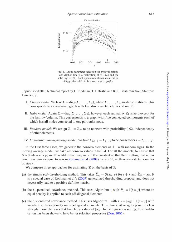
To select a value of λ that will generalize well, we choose λCV = argmaxλαCV (λ). Figure 1shows 20 realizations of crossvalidation for tuning parameter selection. While αCV (λ) appears tobe biased upward for α(λ), we see that the value of λ that maximizes α(λ) is still well estimatedby crossvalidation, especially considering the flatness of α(λ) around the maximum.

5. EMPIRICAL STUDY5·1. Simulation

To evaluate the performance of our covariance estimator, which we will refer to as the�1-penalized covariance method, we generate X1, . . . , Xn ∼ Np(0, �), where � is a sparsesymmetric positive semidefinite matrix. We take n = 200 and p= 100 and consider three typesof covariance graphs, corresponding to different sparsity patterns, considered for example in an

at University of G



Dow

nloaded from



0·00 0·02 0·04 0·06 0·08 0·10

−14·75

−14·65

Crossvalidation

λ

Log

likel

ihoo

d

Fig. 1. Tuning parameter selection via crossvalidation.Each dashed line is a realization of αCV (λ) and thesolid line is α(λ). Each open circle shows a realization

of λCV ; the solid circle shows argmaxλα(λ).

unpublished 2010 technical report by J. Friedman, T. J. Hastie and R. J. Tibshirani from StanfordUniversity:

I. Cliques model: We take � = diag(�1, . . . , �5), where �1, . . . , �5 are dense matrices. Thiscorresponds to a covariance graph with five disconnected cliques of size 20.

II. Hubs model: Again � = diag(�1, . . . , �5), however each submatrix �k is zero except forthe last row/column. This corresponds to a graph with five connected components each ofwhich has all nodes connected to one particular node.

III. Random model: We assign �i j =� j i to be nonzero with probability 0·02, independentlyof other elements.

IV. First-order moving average model: We take �i,i−1 =�i−1,i to be nonzero for i = 2, . . . , p.

In the first three cases, we generate the nonzero elements as ±1 with random signs. In themoving average model, we take all nonzero values to be 0·4. For all the models, to ensure thatS � 0 when n > p, we then add to the diagonal of � a constant so that the resulting matrix hascondition number equal to p as in Rothman et al. (2008). Fixing �, we then generate ten samplesof size n.

We compare three approaches for estimating � on the basis of S:

(a) the simple soft-thresholding method. This takes �i j = S(Si j , c) for i |= j and �i i = Sii . Itis a special case of Rothman et al.’s (2009) generalized thresholding proposal and does notnecessarily lead to a positive definite matrix;

(b) the �1-penalized covariance method. This uses Algorithm 1 with Pi j = 1{i |= j} where anequal penalty is applied to each off-diagonal element;

(c) the �1-penalized covariance method. This uses Algorithm 1 with Pi j = |Si j |−11{i |= j} withan adaptive lasso penalty on off-diagonal elements. This choice of weights penalizes lessstrongly those elements that have large values of |Si j |. In the regression setting, this modifi-cation has been shown to have better selection properties (Zou, 2006).

at University of G



Dow

nloaded from



We evaluate each method on the basis of its ability to correctly identify which elements of �

are zero and on its closeness to � based on both the root-mean-square error, ‖� −�‖F/p, andentropy loss, − log det(��−1)+ tr(��−1)− p. The latter is a natural measure for comparingcovariance matrices and has been used in this context by Huang et al. (2006).

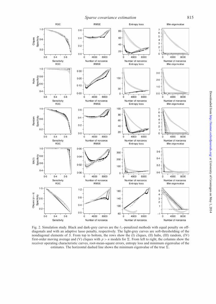
The first four rows of Fig. 2 show how the methods perform under the models for �

described above. We vary c and λ to produce a wide range of sparsity levels. From the receiveroperating characteristic curves, we find that simple soft-thesholding identifies the correct zeroswith comparable accuracy to the �1-penalized covariance approaches (b) and (c). Relatedly, J.Friedman, T. J. Hastie and R. J. Tibshirani, in their 2010 technical report, observe with surprisethe effectiveness of soft-thresholding of the empirical correlation matrix for identifying the zerosin the inverse covariance matrix. In terms of root-mean-square error, all three methods performsimilarly in the cliques model (I) and random model (III). In both these situations, method (b)dominates in the denser realm while method (a) does best in the sparser realm. In the movingaverage model (IV), both soft-thresholding (a) and the adaptive �1-penalized covariance method(c) do better in the sparser realm, with the latter attaining the lowest error. For the hubs model(II), �1-penalized covariance (b) attains the best root-mean-square error across all sparsity levels.In terms of entropy loss there is a pronounced difference between the �1-penalized covariancemethods and soft-thresholding. In particular, we find that the former methods get much closerto the truth in this sense than soft-thresholding in all four cases. This behaviour reflects thedifference in nature between minimizing a penalized Frobenius distance, as is done withsoft-thresholding, and minimizing a penalized negative loglikelihood, as in (1). The rightmostplot shows that for the moving average model (IV) soft-thresholding produces covarianceestimates that are not positive semidefinite for some sparsity levels. When the estimate is notpositive definite, we do not plot the entropy loss. In contrast, the �1-penalized covariance methodis guaranteed to produce a positive definite estimate regardless of the choice of P .

The bottom row of Fig. 2 shows the performance of the �1-penalized covariance method whenS is not full rank. In particular, we take n = 50 and p= 100. The receiver operating characteristiccurves for all three methods decline greatly in this case, reflecting the difficulty of estimationwhen p > n. Despite trying a range of values of λ, we find that the �1-penalized covariancemethod does not produce a uniform range of sparsity levels, but rather jumps from being about33% zero to 99% zero. As with model (IV), we find that soft-thresholding leads to estimates thatare not positive semidefinite, in this case for a wide range of sparsity levels.

5·2. Cell signalling dataset

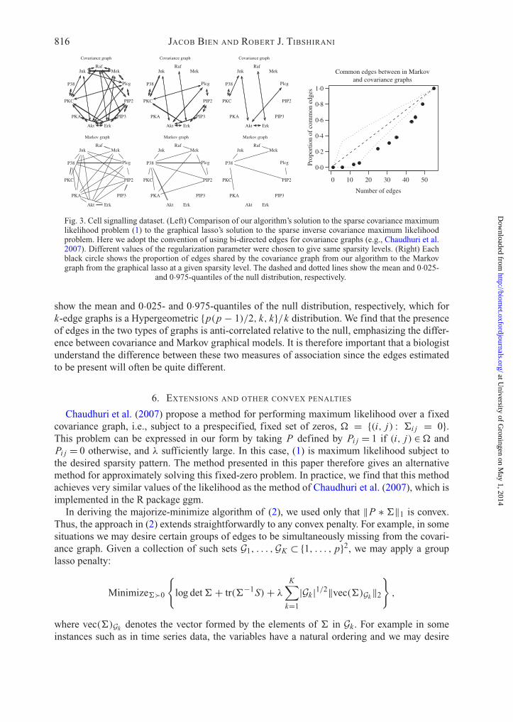
We apply our �1-penalized covariance method to a dataset that has previously been used inthe sparse graphical model literature (Friedman et al., 2007). The data consist of flow cytometrymeasurements of the concentrations of p= 11 proteins in n = 7466 cells (Sachs et al., 2005).Figure 3 compares the covariance graphs learned by the �1-penalized covariance method to theMarkov network learned by the graphical lasso (Friedman et al., 2007). The two types of graphhave different interpretations: if the estimated covariance graph has a missing edge between twoproteins, then we are stating that the concentration of one protein gives no information aboutthe concentration of another. On the other hand, a missing edge in the Markov network meansthat, conditional on all other proteins’ concentrations, the concentration of one protein gives noinformation about the concentration of another. Both of these statements assume that the data aremultivariate Gaussian. The right panel of Fig. 3 shows the extent to which similar protein pairs areidentified by the two methods for a series of sparsity levels. We compare the observed proportionof co-occurring edges to a null distribution in which two graphs are selected independently fromthe uniform distribution of graphs having a certain number of edges. The dashed and dotted lines

at University of G



Dow

nloaded from



Fig. 2. Simulation study. Black and dark-grey curves are the �1-penalized methods with equal penalty on off-diagonals and with an adaptive lasso penalty, respectively. The light-grey curves are soft-thresholding of thenondiagonal elements of S. From top to bottom, the rows show the (I) cliques, (II) hubs, (III) random, (IV)first-order moving average and (V) cliques with p > n models for �. From left to right, the columns show thereceiver operating characteristic curves, root-mean-square errors, entropy loss and minimum eigenvalue of the

estimates. The horizontal dashed line shows the minimum eigenvalue of the true �.

at University of G



Dow

nloaded from



RafMek

Plcg

PIP2

PIP3

ErkAkt

PKA

PKC

P38

Jnk

Covariance graph

RafMek

Plcg

PIP2

PIP3

ErkAkt

PKA

PKC

P38

Jnk

Markov graph

RafMek

Plcg

PIP2

PIP3

ErkAkt

PKA

PKC

P38

Jnk

Covariance graph

RafMek

Plcg

PIP2

PIP3

ErkAkt

PKA

PKC

P38

Jnk

Markov graph

RafMek

Plcg

PIP2

PIP3

ErkAkt

PKA

PKC

P38

Jnk

Covariance graph

RafMek

Plcg

PIP2

PIP3

ErkAkt

PKA

PKC

P38

Jnk

Markov graph

0 10 20 30 40 50

0·0

0·2

0·4

0·6

0·8

1·0

Common edges between in Markovand covariance graphs

Number of edges

Prop

ortio

n of

com

mon

edg

es

Fig. 3. Cell signalling dataset. (Left) Comparison of our algorithm’s solution to the sparse covariance maximumlikelihood problem (1) to the graphical lasso’s solution to the sparse inverse covariance maximum likelihoodproblem. Here we adopt the convention of using bi-directed edges for covariance graphs (e.g., Chaudhuri et al.2007). Different values of the regularization parameter were chosen to give same sparsity levels. (Right) Eachblack circle shows the proportion of edges shared by the covariance graph from our algorithm to the Markovgraph from the graphical lasso at a given sparsity level. The dashed and dotted lines show the mean and 0·025-

and 0·975-quantiles of the null distribution, respectively.

show the mean and 0·025- and 0·975-quantiles of the null distribution, respectively, which fork-edge graphs is a Hypergeometric {p(p − 1)/2, k, k}/k distribution. We find that the presenceof edges in the two types of graphs is anti-correlated relative to the null, emphasizing the differ-ence between covariance and Markov graphical models. It is therefore important that a biologistunderstand the difference between these two measures of association since the edges estimatedto be present will often be quite different.

6. EXTENSIONS AND OTHER CONVEX PENALTIES

Chaudhuri et al. (2007) propose a method for performing maximum likelihood over a fixedcovariance graph, i.e., subject to a prespecified, fixed set of zeros, � = {(i, j) : �i j = 0}.This problem can be expressed in our form by taking P defined by Pi j = 1 if (i, j) ∈� andPi j = 0 otherwise, and λ sufficiently large. In this case, (1) is maximum likelihood subject tothe desired sparsity pattern. The method presented in this paper therefore gives an alternativemethod for approximately solving this fixed-zero problem. In practice, we find that this methodachieves very similar values of the likelihood as the method of Chaudhuri et al. (2007), which isimplemented in the R package ggm.

In deriving the majorize-minimize algorithm of (2), we used only that ‖P ∗�‖1 is convex.Thus, the approach in (2) extends straightforwardly to any convex penalty. For example, in somesituations we may desire certain groups of edges to be simultaneously missing from the covari-ance graph. Given a collection of such sets G1, . . . ,GK ⊂ {1, . . . , p}2, we may apply a grouplasso penalty:

Minimize��0

{log det � + tr(�−1S)+ λ

K∑k=1

|Gk |1/2‖vec(�)Gk‖2}

,

where vec(�)Gk denotes the vector formed by the elements of � in Gk . For example in someinstances such as in time series data, the variables have a natural ordering and we may desire

at University of G



Dow

nloaded from



a banded sparsity pattern (Rothman et al., 2010). In such a case, one could take Gk = {(i, j) :|i − j | = k} for k = 1, . . . , p − 1. Estimating the kth band as zero would correspond to a modelin which a variable is marginally independent of the variable k time units earlier.

As another example, we could take Gk = {(k, i) : i |= k} ∪ {(i, k) : i |= k} for k = 1, . . . , p. Thisencourages a node-sparse graph considered by J. Friedman, T. J. Hastie and R. J. Tibshirani, intheir 2010 technical report, in the case of the inverse covariance matrix. Estimating �i j = 0 forall (i, j) ∈ Gk corresponds to the model in which variable k is independent of all others. It shouldbe noted however that a variable’s being marginally independent of all others is equivalent to itsbeing conditionally independent of all others. Therefore, if node-sparsity in the covariance graphis the only goal, i.e., no other penalties on � are present, a better procedure would be to applythis group lasso penalty to the inverse covariance, thereby admitting a convex problem.

We conclude with an extension that may be worth pursuing. A difficulty with (1) is that it isnot convex and therefore any algorithm that attempts to solve it may converge to a suboptimallocal minimum. Exercise 7.4 of Boyd & Vandenberghe (2004), on p. 394, remarks that the log-likelihood �(�) is concave on the convex set C0 = {� : 0≺� � 2S}. This fact can be verified bynoting that over this region the positive curvature of tr(�−1S) exceeds the negative curvature oflog det �. This suggests a related estimator that is the result of a convex optimization problem:let �c denote a solution to

Minimize0≺��2S

{log det � + tr(�−1S)+ λ‖P ∗�‖1

}. (5)

While of course we cannot in general expect �c to be a solution to (1), adding this con-straint may not be unreasonable. In particular, if n, p→∞ with p/n→ y ∈ (0, 1), then bya result of Silverstein (1985), λmin(�

−1/20 S�

−1/20 )→ (1− y1/2)2 almost surely, where S ∼

Wishart(�0, n). It follows that the constraint �0 � 2S will hold almost surely in this limit if(1− y1/2)2 > 0·5, i.e., y < 0·085. Thus, in the regime that n is large and p does not exceed0·085n, the constraint set of (5) contains the true covariance matrix with high probability.

ACKNOWLEDGEMENT

We thank Ryan Tibshirani and Jonathan Taylor for useful discussions and two anonymousreviewers and an associate editor for helpful comments. Jacob Bien was supported by the UrbanekFamily Stanford Graduate Fellowship and the Lieberman Fellowship; Robert Tibshirani was par-tially supported by the National Science Foundation and the National Institutes of Health, U.S.A.

SUPPLEMENTARY MATERIAL

Supplementary material available at Biometrika online includes a simulation evaluating theperformance of our estimator as n increases.

APPENDIX 1

Convex plus concave

Examining the objective of problem (1) term by term, we observe that log det � is concave whiletr(�−1S) and λ‖�‖1 are convex in �. The second derivative of log det � is −�−2, which is negative def-inite, from which it follows that log det � is concave. As shown in Example 3.4 of Boyd & Vandenberghe(2004), on p. 76, X T

i �−1 Xi is jointly convex in Xi and �. Since tr(�−1S)= n−1

∑ni=1 X T

i �−1 Xi , it follows

that tr(�−1S) is the sum of convex functions and therefore is itself convex.

at University of G



Dow

nloaded from



APPENDIX 2

Justifying the Lipschitz claim

Let L(�)= tr(�−10 �)+ tr(�−1S) denote the differentiable part of the majorizing function of (1).

We wish to prove that d L(�)/d� =�−10 −�−1S�−1 is Lipschitz continuous over the region of the

optimization problem. Since this is not the case for λmin(�)→ 0, we begin by showing that the constraintregion can be restricted to � � δ Ip.

PROPOSITION 1. Let � be an arbitrary positive definite matrix, e.g., � = S. Problem (1) is equivalentto

Minimize��δ Ip

{log det � + tr(�−1S)+ λ‖P ∗�‖1

}for some δ > 0 that depends on λmin(S) and f (�).

Proof. Let g(�)= log det � + tr(�−1S) denote the differentiable part of the objective functionf (�)= g(�)+ λ‖P ∗�‖1, and let � =∑p

i=1 λi ui uTi be the eigendecomposition of � with λ1 � · · ·�

λp.Given a point � with f (�) <∞, we can write (1) equivalently as

Minimize f (�) subject to � � 0, f (�) � f (�).

We show in what follows that the constraint f (�) � f (�) implies � � δ Ip for some δ > 0.Now, g(�)=∑p

i=1 log λi + uTi Sui/λi =

∑pi=1 h(λi ; uT

i Sui ), where h(x; a)= log x + a/x . For a > 0,the function h has a single stationary point at a, where it attains a minimum value of log a + 1, haslimx→0+ h(x; a)=+∞ and limx→∞ h(x; a)=+∞, and is convex for x � 2a. Also, h(x; a) is increas-ing in a for all x > 0. From these properties and the fact that λmin(S)=min‖u‖2=1 uT Su, it follows that

g(�) �p∑

i=1

h{λi ; λmin(S)}� h{λp; λmin(S)} +p−1∑i=1

h{λmin(S); λmin(S)}

= h{λp; λmin(S)} + (p − 1){log λmin(S)+ 1}.

Thus, f (�) � f (�) implies g(�) � f (�) and so

h{λp; λmin(S)} + (p − 1){log λmin(S)+ 1}� f (�).

This constrains λp to lie in an interval [δ−, δ+]= {λ : h{λ; λmin(S)}� c}, where c= f (�)− (p −1){log λmin(S)+ 1} and δ−, δ+ > 0. We compute δ− using Newton’s method. To see that δ− > 0, note thath is continuous and monotone decreasing on (0, a) and limx→0+ h(x; a)=+∞.

As λmin(S) increases, [δ−, δ+] becomes narrower and more shifted to the right. The interval also narrowsas f (�) decreases.

For example, we may take � = diag(S11, . . . , Spp) and P = 11T − Ip, which yields

h{λp, λmin(S)}�p∑

i=1

log{Sii/λmin(S)} + log λmin(S)+ 1.�

We next show that d L(�)/d� =�−10 −�−1S�−1 is Lipschitz continuous on � � δ Ip by bounding

its first derivative. Using the product rule for matrix derivatives, we have

d

d�(�−1

0 −�−1S�−1)=−(�−1S ⊗ Ip)(−�−1 ⊗�−1)− (Ip ⊗�−1){(Ip ⊗ S)(−�−1 ⊗�−1)}

= (�−1S�−1)⊗�−1 +�−1 ⊗ (�−1S�−1).

at University of G



Dow

nloaded from



We bound the spectral norm of this matrix:∥∥∥∥ d

d�

d L

d�

∥∥∥∥2

� ‖(�−1S�−1)⊗�−1‖2 + ‖�−1 ⊗�−1S�−1‖2

� 2‖�−1S�−1‖2‖�−1‖2

� 2‖S‖2‖�−1‖32.

The first inequality follows from the triangle inequality; the second uses the fact that the eigenvalues ofA ⊗ B are the pairwise products of the eigenvalues of A and B; the third uses the sub-multiplicativity ofthe spectral norm. Finally, � � δ Ip implies that �−1 � δ−1 Ip, from which it follows that∥∥∥∥ d

d�

d L

d�

∥∥∥∥2

� 2‖S‖2δ−3.

APPENDIX 3

Alternating direction method of multipliers for solving (3)

To solve (3), we repeat until convergence:

1. diagonalize {� − t (�−10 −�−1S�−1)+ ρk − Y k}/(1+ ρ)=U DU T;

2. �k+1←U DδU T where Dδ = diag{max(Dii , δ)};3. k+1← S{�k+1 + Y k/ρ, (λ/ρ)P}, i.e., soft-threshold elementwise;

4. Y k+1← Y k + ρ(�k+1 −k+1).

REFERENCES

AN, L. & TAO, P. (2005). The dc (difference of convex functions) programming and dca revisited with dc models ofreal world nonconvex optimization problems. Ann. Oper. Res. 133, 23–46.

ARGYRIOU, A., HAUSER, R., MICCHELLI, C. & PONTIL, M. (2006). A dc-programming algorithm for kernel selection.In Proc. 23rd Int. Conf. Mach. Learn. New York: Association for Computing Machinery.

BANERJEE, O., EL GHAOUI, L. E. & D’ASPREMONT, A. (2008). Model selection through sparse maximum likelihoodestimation for multivariate Gaussian or binary data. J. Mach. Learn. Res. 9, 485–516.

BECK, A. & TEBOULLE, M. (2009). A fast iterative shrinkage-thresholding algorithm for linear inverse problems. SIAMJ. Imag. Sci. 2, 183–202.

BOYD, S. & VANDENBERGHE, L. (2004). Convex Optimization. Cambridge: Cambridge University Press.BOYD, S., PARIKH, N., CHU, E., PELEATO, B. & ECKSTEIN, J. (2011). Distributed optimization and statistical learning

via the alternating direction method of multipliers. Foundat. Trends Mach. Learn. 3, 1–124.BUTTE, A. J., TAMAYO, P., SLONIM, D., GOLUB, T. R. & KOHANE, I. S. (2000). Discovering functional relationships

between RNA expression and chemotherapeutic susceptibility using relevance networks. Proc. Nat. Acad. Sci.U.S.A. 97, 12182–6.

CHAUDHURI, S., DRTON, M. & RICHARDSON, T. S. (2007). Estimation of a covariance matrix with zeros. Biometrika94, 199–216.

DE LEEUW, J. & MAIR, P. (2009). Multidimensional scaling using majorization: SMACOF in R. J. Statist. Software31, 1–30.

DEMPSTER, A. P. (1972). Covariance selection. Biometrics 28, 157–75.DRTON, M. & RICHARDSON, T. S. (2008). Graphical methods for efficient likelihood inference in Gaussian covariance

models. J. Mach. Learn. Res. 9, 893–914.FAZEL, M., HINDI, H. & BOYD, S. (2003). Log-det heuristic for matrix rank minimization with applications to Han-

kel and Euclidean distance matrices. In Am. Contr. Conf., 2003. Proc. 2003, vol. 3. Institute of Electrical andElectronics Engineers.

FRIEDMAN, J.,HASTIE, T. J. & TIBSHIRANI, R. J. (2007). Sparse inverse covariance estimation with the graphical lasso.Biostatistics 9, 432–41.

HORST, R. & THOAI, N. V. (1999). Dc programming: Overview. J. Optimiz. Theory Appl. 103, 1–43.HUANG, J., LIU, N., POURAHMADI, M. & LIU, L. (2006). Covariance matrix selection and estimation via penalised

normal likelihood. Biometrika 93, 85.

at University of G



Dow

nloaded from



HUNTER, D. R. & LI, R. (2005). Variable selection using MM algorithms. Ann. Statist. 33, 1617–42.KHARE, K. & RAJARATNAM, B. (2011). Wishart distributions for decomposable covariance graph models. Ann. Statist.

39, 514–55.LAM, C. & FAN, J. (2009). Sparsistency and rates of convergence in large covariance matrix estimation. Ann. Statist.

37, 4254–78.LANGE, K. (2004). Optimization. New York: Springer.MEINSHAUSEN, N. & BUHLMANN, P. (2006). High dimensional graphs and variable selection with the lasso. Ann.

Statist. 34, 1436–62.NESTEROV, Y. (2005). Smooth minimization of non-smooth functions. Math. Prog. 103, 127–52.ROTHMAN, A., LEVINA, E. & ZHU, J. (2008). Sparse permutation invariant covariance estimation. Electron. J. Statist.

2, 494–515.ROTHMAN, A., LEVINA, E. & ZHU, J. (2010). A new approach to Cholesky-based covariance regularization in high

dimensions. Biometrika 97, 539.ROTHMAN, A. J., LEVINA, E. & ZHU, J. (2009). Generalized thresholding of large covariance matrices. J. Am. Statist.

Assoc. 104, 177–86.SACHS, K., PEREZ, O., PE’ER, D., LAUFFENBURGER, D. & NOLAN, G. (2005). Causal protein-signaling networks

derived from multiparameter single-cell data. Science 308, 523–9.SILVERSTEIN, J. (1985). The smallest eigenvalue of a large dimensional Wishart matrix. Ann. Prob. 13, 1364–8.SRIPERUMBUDUR, B. & LANCKRIET, G. (2009). On the convergence of the concave-convex procedure. In Advances

in Neural Information Processing Systems, 22. Ed. Y. Bengio, D. Schuurmans, J. Lafferty, C. K. I. Williams &A. Culotta, pp. 1759–67.

TIBSHIRANI, R. (1996). Regression shrinkage and selection via the lasso. J. R. Statist. Soc. B 58, 267–88.YUAN, M. & LIN, Y. (2007). Model selection and estimation in the Gaussian graphical model. Biometrika 94, 19–35.YUILLE, A. L. & RANGARAJAN, A. (2003). The concave–convex procedure. Neural Comp. 15, 915–36.ZHANG, T. (2010). Analysis of multi-stage convex relaxation for sparse regularization. J. Mach. Learn. Res. 11,

1081–107.ZOU, H. (2006). The adaptive lasso and its oracle properties. J. Am. Statist. Assoc. 101, 1418–29.

[Received December 2010. Revised July 2011]

at University of G



Dow

nloaded from


Documents

Sparse estimation of a covariance matrix