Embed Size (px)
Citation preview


Sommario
L'organizzazione gerarchica dei sistemi di memoria e di comunicazione e la disponibilità di
molte unità di calcolo inuiscono notevolmente sulle prestazioni di un algoritmo. Il loro
eciente utilizzo è limitato dalle dierenti congurazioni che possono assumere. È cru-
ciale, per motivi economici e di portabilità, che gli algoritmi si adattino allo spettro delle
piattaforme esistenti e che la procedura di adattamento sia il più possibile automatizzata.
L'adattività può essere raggiunta sia tramite algoritmi aware, che utilizzano esplicitamen-
te opportuni parametri architetturali, sia tramite algoritmi oblivious, la cui sequenza di
operazioni è indipendente dalle caratteristiche dell'architettura sottostante. Gli algoritmi
oblivious esibiscono spesso prestazioni ottime su diverse architetture e sono attrattivi so-
prattutto nei contesti in cui i parametri architetturali sono dicili da stimare o non sono
noti.
Questa tesi si focalizza sullo studio degli algoritmi oblivious con due obiettivi principali:
l'indagine delle potenzialità e limitazioni delle computazioni oblivious e l'introduzione del
concetto di algoritmo oblivious in un sistema parallelo.
Inizialmente, vengono arontate varie problematiche legate all'esecuzione di algoritmi
cache-oblivious per permutazioni razionali, le quali rappresentano un'importante classe di
permutazioni che include la trasposizione di matrici e il bit-reversal di vettori. Si dimostra
un lower bound, valido anche per algoritmi cache-aware, sul numero di operazioni macchina
necessarie per eseguire una permutazione razionale assumendo un numero ottimo di accessi
alla memoria. Quindi, si descrive un algoritmo cache-oblivious che esegue qualsiasi permu-
tazione razionale e che richiede un numero ottimo di operazioni macchina e di accessi alla
memoria, assumendo l'ipotesi di tall-cache. Inne, si dimostra che per certe famiglie di per-
mutazioni razionali (tra cui la trasposizione e il bit-reversal) non può esistere un algoritmo
cache-oblivious che richieda un numero ottimo di accessi alla memoria per tutti i valori dei
parametri della cache, mentre esiste un algoritmo cache-aware con tali caratteristiche.
Nella tesi viene poi introdotto il framework network-oblivious per lo studio di algoritmi
oblivious in un sistema parallelo. Il framework esplora lo sviluppo di algoritmi paralle-
li di tipo bulk-synchronous che, senza usare parametri dipendenti dalla macchina, hanno
prestazioni ecienti su macchine parallele con dierenti gradi di parallelismo e valori di ban-
da/latenza. Vengono inoltre forniti algoritmi network-oblivious per alcuni problemi chiave
(moltiplicazione e trasposizione di matrici, trasformata discreta di Fourier, ordinamento) e
viene presentato un risultato di impossibilità sull'esecuzione di algoritmi network-oblivious
per la trasposizione di matrici che ricorda quello ottenuto per le permutazioni razionali.
Inne, per mostrare ulteriormente le potenzialità del framework, vengono presentati
algoritmi network-oblivious ottimi per eseguire un'ampia classe di computazioni risolvibili
tramite il paradigma di programmazione ad eliminazione gaussiana, tra cui il calcolo dei
cammini minimi in un grafo, l'eliminazione gaussiana senza pivoting e la moltiplicazione di
matrici.


Abstract
The hierarchical organization of the memory and communication systems and the availabil-
ity of numerous processing units play an important role in the performance of algorithms.
Their actual exploitation is made hard by the dierent congurations they may assume. It
is crucial, for economical and portability issues, that algorithms adapt to a wide spectrum of
executing platforms, possibly in an automatic fashion. Adaptivity can be achieved through
either aware algorithms, which make explicit use of suitable architectural parameters, or
oblivious algorithms, whose sequence of operations is independent of the characteristics
of the underlying architecture. Oblivious algorithms are more desirable in contexts where
architectural parameters are unknown and hard to estimate, and, in some cases, they still
exhibit optimal performance across dierent architectures.
This thesis focuses on the study of oblivious algorithms pursuing two main objectives:
the investigation of the potentialities and intrinsic limitations of oblivious computations in
comparison with aware ones, and the introduction of the notion of oblivious algorithm in
the parallel setting.
We study various aspects concerning the execution of cache-oblivious algorithms for ra-
tional permutations, an important class of permutations including matrix transposition and
the bit-reversal of a vector. We provide a lower bound, which is also valid for cache-aware
algorithms, on the work complexity required by the execution of a rational permutation
with an optimal cache complexity. Then, we develop a cache-oblivious algorithm perform-
ing any rational permutation, which exhibits optimal work and cache complexities under
the tall-cache assumption. We then show that for certain families of rational permutations
(including transposition and bit-reversal) no cache-oblivious algorithm can exhibit optimal
cache complexity for all values of the cache parameters, while there exists a cache-aware
algorithm with this property.
We introduce the network-oblivious framework for the study of oblivious algorithms
in the parallel setting. This framework explores the design of bulk-synchronous parallel
algorithms that, without resorting to parameters for tuning the performance on the target
platform, can execute eciently on parallel machines with dierent degree of parallelism
and bandwidth/latency characteristics. We illustrate the framework by providing optimal
network-oblivious algorithms for a few key problems (i.e., matrix multiplication and trans-
position, discrete Fourier transform and sorting) and by presenting an impossibility result
on the execution of network-oblivious algorithms for matrix transposition, which is similar,
in spirit, to the one provided for rational permutations.
Finally, we present a number of network-oblivious algorithms, which exhibit optimal
communication and computation complexities, for solving a wide class of computations
encompassed by the Gaussian Elimination Paradigm, including all-pairs shortest paths,
Gaussian elimination without pivoting and matrix multiplication.


Ringraziamenti
Ecco, nalmente, la pagina che ho desiderato a lungo di scrivere e che sicuramente sarà la
più letta. Negli anni trascorsi come dottorando nel Dipartimento di Ingegneria Informatica
ho incontrato persone eccezionali con cui ho condiviso bellissimi momenti e che mi han-
no aiutato a crescere professionalmente e umanamente. Sono riconoscente a tutte queste
persone e ad alcune di loro voglio dedicare un pensiero.
Il primo grazie va ad Andrea. Mi ritengo fortunato ad aver avuto Andrea come advisor
in questi anni: è sempre stato disponibile a consigliarmi e ad aiutarmi, facendo sempre
più del suo dovere. Lo ringrazio soprattutto per aver cercato di migliorare, e sopportato,
il mio modo non lineare di pensare accompagnato da un usso impulsivo di parole. Rin-
grazio poi Geppino per il suo corso di Fondamenti di Informatica II, che mi ha introdotto
all'algoritmica, e per essere stato un ottimo co-advisor.
Un ringraziamento speciale va alla vecchia guardia di dottorandi e assegnisti del labo-
ratorio ACG: Alberto B., Fabio, Francesco, Marco e Paolo; con loro ho condiviso i momenti
migliori e più allegri del mio dottorato e stretto bellissime amicizie. In particolare sono
grato a Fabio per le lunghe chiacchierate e per avermi contagiato con la sua passione per
la ricerca (prima o poi pubblicheremo qualcosa insieme!), e a Marco per avermi ricordato
che le risorse della Terra sono nite. Sono poi riconoscente a Alberto P., Carlo, Enoch,
Gianfranco, Mattia e Michele per le interessanti discussioni (quelle di Gianfranco anche
particolarmente lunghe) e ad Alessandra, il cuore della Scuola di Dottorato, per la sua
gentilezza e disponibilità.
Non posso dimenticare Bruno che con tutta la sua energia mi ha permesso di capire e
apprezzare gli Stati Uniti D'America.
Un grazie speciale va ad Adriano per essere stato un vero amico in tutti questi anni
e per tutte le birre bevute insieme. Ringrazio poi Alberto e Martina per aver condiviso
l'appartamento, ma soprattutto per aver sopportato i miei go tentativi di far saltare la
pasta in padella.
Inne, voglio dire grazie alle tre persone più importanti della mia vita, anche se non
sono in grado di esprimere quello che sono stati e hanno fatto per me: senza di loro non
avrei mai provato quei sentimenti di cui ora non posso più fare a meno. A mia mamma
Fanny e a mio papà Giuliano: il vostro amore è stato un punto di riferimento e un aiuto in
tutti questi anni; senza di voi, non sarei arrivato n qui. E ad Elisa, la mia futura moglie:
grazie per avermi sempre ascoltato, consigliato ed essere stata al mio anco; grazie a te ora
sono Felice.


Acknowledgements
It is very dicult for me to translate my feelings into English, but I would like to thank the
few people that cannot understand my language. I'm grateful to Vijaya Ramachandran for
inviting me to spend some months at the University of Texas at Austin and for the useful
discussions. I also thank Rezaul Alam Chowdhury for his collaboration.


Contents
Chapter 1: Introduction 1
Chapter 2: Models for Memory and Communication Hierarchies 9
2.1 Models for memory hierarchy . . . . . . . . . . . . . . . . . . . . . . 10
2.1.1 External Memory model . . . . . . . . . . . . . . . . . . . . . 11
2.1.2 Ideal Cache model . . . . . . . . . . . . . . . . . . . . . . . . 12
2.2 Models for communication hierarchy . . . . . . . . . . . . . . . . . . 15
2.2.1 D-BSP model . . . . . . . . . . . . . . . . . . . . . . . . . . . 17
Chapter 3: Limits of Cache-Oblivious Rational Permutations 21
3.1 Rational permutations . . . . . . . . . . . . . . . . . . . . . . . . . . 23
3.2 Lower bounds . . . . . . . . . . . . . . . . . . . . . . . . . . . . . . . 26
3.3 Cache-oblivious algorithm for rational permutations . . . . . . . . . . 33
3.3.1 Computing the values of a rational permutation . . . . . . . . 33
3.3.2 Performing a rational permutation . . . . . . . . . . . . . . . 35
3.4 Limits of cache-oblivious rational permutations . . . . . . . . . . . . 39
3.4.1 The simulation technique . . . . . . . . . . . . . . . . . . . . . 40
3.4.2 Impossibility result for rational permutations . . . . . . . . . . 42
Chapter 4: Network-Oblivious Algorithms 47
4.1 The framework . . . . . . . . . . . . . . . . . . . . . . . . . . . . . . 49
4.2 Algorithms for key problems . . . . . . . . . . . . . . . . . . . . . . . 54
4.2.1 Matrix multiplication . . . . . . . . . . . . . . . . . . . . . . . 54
4.2.2 Matrix transposition . . . . . . . . . . . . . . . . . . . . . . . 61
4.2.3 Impossibility result for matrix transposition . . . . . . . . . . 63
4.2.4 FFT . . . . . . . . . . . . . . . . . . . . . . . . . . . . . . . . 65
4.2.5 Sorting . . . . . . . . . . . . . . . . . . . . . . . . . . . . . . . 67
Chapter 5: Network-Oblivious Algorithms for GEP 71
5.1 Preliminaries . . . . . . . . . . . . . . . . . . . . . . . . . . . . . . . 72
5.1.1 Denition of GEP . . . . . . . . . . . . . . . . . . . . . . . . . 72
i

ii Contents
5.1.2 Previous cache-oblivious and parallel implementations of GEP 73
5.2 Network-Oblivious Algorithms . . . . . . . . . . . . . . . . . . . . . . 75
5.2.1 N-GEP . . . . . . . . . . . . . . . . . . . . . . . . . . . . . . . 76
5.2.2 εN-GEP . . . . . . . . . . . . . . . . . . . . . . . . . . . . . . 90
5.2.3 PN-GEP . . . . . . . . . . . . . . . . . . . . . . . . . . . . . . 101
Chapter 6: Conclusions 103
6.1 Summary . . . . . . . . . . . . . . . . . . . . . . . . . . . . . . . . . 103
6.2 Further research . . . . . . . . . . . . . . . . . . . . . . . . . . . . . . 105
Appendix A: Properties of Function f(x) 107
Appendix B: Pseudocode of PI-GEP1 and PI-GEP2 111
Bibliography 115

Chapter 1
Introduction
You have to be fast on your feet and
adaptive or else a strategy is useless.
(Charles de Gaulle)
Since the advent of computers, the request of computational power from applica-
tions has been continuously growing and has increased signicantly in the last twenty
years with the emergence of novel applications in computational sciences as well as
in many other contexts. This phenomenon has posed formidable challenges to both
computer architects and software/algorithm designers, and much progress has been
made in the development of architectures, algorithms and compilers. Nevertheless,
the potential power of actual platforms can hardly be fully exploited.
One of the main reasons which limit the eciency of an application is the so-
called memory wall. While the clock speed of functional units has been growing
exponentially, at least until recent years when physical limits have been approached
[ABC+06], the advances in the realization of memory supports have been less impres-
sive. This phenomenon has increased the gap in eciency between functional units
and memory supports, which is the main cause of ineciency in sequential applica-
tions [Bac78]. Several architectural approaches have been adopted to mitigate the
impact of this gap. The traditional approach consists in the introduction, between
the main memory and the functional unit(s), of several levels of caches, which are
fast yet small memories [HP06]. The main justication for this hierarchical orga-
nization of the memory system is that an algorithm typically reuses small sets of
data within relatively short time intervals, a property referred to as temporal locality
of reference. Thus, the time required for retrieving these data can be decreased if
they are stored in faster caches. Another important aspect is the movement of data
in batches of contiguous segments (blocks) between adjacent levels of the memory
hierarchy. The motivation is that an algorithm usually requires data that reside in
1

2 Chapter 1. Introduction
contiguous memory locations within a short time interval, a property referred to as
spatial locality of reference. Since accessing all data in one shot is less expensive than
performing several independent accesses, it is convenient to move data in blocks.
A number of compilers, prefetching techniques and runtime speculative analy-
ses [KA02, HP06] have been introduced to reduce the programmers' eort when
dealing with the memory hierarchy. Although, these approaches yield some perfor-
mance improvements, more substantial optimizations can be made at the algorithm
design level. For this reason, a number of computational models have been intro-
duced to help programmers develop algorithms which perform eciently in memory
hierarchies (see [Vit01, MSS03] and references therein). These models aim at rep-
resenting only the most important features of the hierarchy in order to simplify the
design process. Examples are the External Memory model of Aggarwal and Vitter
[AV88] and the Ideal Cache model of Frigo et al. [FLPR99]. The rst represents
a disk-RAM hierarchy [Vit01, GVW96, SN96], while the second a RAM-cache one
[Dem02, ABF05].
As already noted, the clock speed cannot be increased indenitely since the nite
speed of light and thermodynamic laws impose physical limitations. A natural solu-
tion to increase the number of operations executed per time unit is the resort to par-
allel architectures. Parallelism has been studied for decades [JáJ92, Lei92, CSG98],
and has been explored at the bit level, instruction level, and thread level. Many
compilers [Wol96] and languages [MHS05] have been proposed to help programmers
extract parallelism automatically from their applications, but they do not always
provide optimal solutions. Indeed, the best approach is to expose parallelism explic-
itly at the algorithm design level. However, there is practical evidence that this is
not an easy task. Furthermore, the situation is made more complex by the lack of
a widely accepted model of computation which strikes a good balance between the
conicting requirements of usability, eectiveness and portability. In the sequential
setting one such model has been constituted for many years by the Random Access
Machine based on the Von Neumann organization [AHU74]. Unfortunately, in the
parallel setting there is still no agreement on a common model for algorithm de-
sign and analysis, although some proposals have received considerable attention and
a broad consensus. Among them we recall the Bulk Synchronous Parallel (BSP)
model by Valiant [Val90] and successive extensions, like the Decomposable-BSP (D-
BSP) model by De la Torre and Kruskal [DlTK96], which have been both extensively
studied (see [BPP07] and references therein).
A major obstacle to the achievement of high performance in parallel architec-
tures, is represented by the cost of communication. Since the relevance of this factor

3
increases with the size of the system, communication will play an even greater role
in future years. Thus, reducing the communication requirements of algorithms is of
paramount importance, if they have to run eciently. The cost of communication is
in general dependent on the distance between the processors involved, and in typ-
ical parallel architectures processors communicate through a hierarchical intercon-
nection featuring dierent bandwidth and latency characteristics at dierent levels.
Thus programs run eciently if they are able to conne data exchanges within small
regions of the interconnection, a property referred to as submachine locality. This
scenario is reected in several models [Lei85, BP97, BP99, ACS90, CKP+96], and
constitute the fundamental grounds upon which the aforementioned D-BSP model,
which eectively describes a very large and signicant class of parallel platforms
[BPP07], has been dened.
Therefore, it is evident that parallelism on the one hand and the hierarchical
organization of the memory and of the interconnection on the other play a key role
in the performance of applications, and their combination has become even more
evident with the advent of Chip Multi-Processors [ONH+96]. As we have already
observed, optimizations based on these factors can be reached, to some extent, by
automatic techniques, but the best results are obtained through a judicious algo-
rithm design process. In aggressive optimizations, an algorithm is tuned to match
almost perfectly the characteristics of the target machine. Although this approach is
common in applications which require expensive or special purpose platforms (such
as IBM BlueGene/L [Aea02] and APE computers for Quantum Chromo Dynam-
ics [BPP+05]), in general it is undesirable for economical and portability reasons.
Moreover, an aggressive optimization could not be possible in scenarios, like grid
environments [FK03], where software may be required to run, for availability or load
management purposes, on widely dierent congurations, which may be revealed
only at runtime. An alternative approach, which is becoming more and more popu-
lar, is provided by adaptive algorithms, that is, algorithms which adapt themselves
to the target machine where they run. We can distinguish two dierent kinds of
adaptive algorithms: aware and oblivious.
Aware adaptive algorithms use machine dependent parameters that are set at run
time to match adaptively the structure of the actual platform. Some libraries that
follow this approach are: Fast Fourier Transform in The West (FFTW ) [FJ98] for
the discrete Fourier transform (DFT), Automatically Tuned Linear Algebra Software
(ATLAS ) [WPD01] for linear algebra problems, Finite-Elements Multifrontal Solver
(FEMS ) [Ber08] for applications based on the Finite-Elements method. The FFTW
library computes a plan for the machine where it is running, which provides informa-

4 Chapter 1. Introduction
tion on how the DFT can be eciently computed on that machine. If the machine
does not change, the plan can be reused for many transforms, amortizing the cost of
plan building. ATLAS is an implementation of a style of performance software pro-
duction called Automated Empirical Optimization of Software (AEOS ) [WPD01]; in
an AEOS-enabled library, many dierent ways of performing a given kernel operation
are supplied, and timers are used to empirically determine which implementation is
best for a given architecture. FEMS is a solver designed for distributed-memory
parallel machines and arranges the computation based on the organization of the
memory system and on the subdivision of processors into clusters.
Oblivious adaptive algorithms are algorithms where no parameters dependent on
machine characteristics need to be tuned to achieve eciency, and still exhibit high
performance on several machines. This tape of algorithms has recently been intro-
duced by Frigo et al. in [FLPR99] through the notion of cache-oblivious algorithms.
These algorithms are designed for the Random Access Machine, but are analyzed
on the Ideal Cache model. Cache-oblivious algorithms are desirable because if op-
timal in the Ideal Cache model they can be proved, under some assumptions, to
be optimal also in multi-level memory hierarchies. Cache-oblivious algorithms have
been proposed for many problems (see [Dem02, ABF05] and references therein), and
they have also been adopted in the commercial software Tokutek [Tok]. Intuitively,
a key paradigm for cache-oblivious algorithms is divide and conquer : problems are
recursively decomposed into smaller problems which, at some point of the recursion,
will t in the cache of the machine. However, it must be said that some problems
can be solved optimally by non-recursive cache-oblivious algorithms.
Although the aware approach in practical settings reaches better results than the
oblivious one [YRP+07], we think that the latter embodies valuable ideas and oppor-
tunities. As noted in [Fri99], with reference to cache-oblivious computations, since
divide and conquer is advantageous for portable high-performance programs, archi-
tectural innovations and compiler techniques to reduce the cost of procedure calls are
to be sought. An improvement in this direction will reduce the practical gap between
oblivious and aware algorithms, and make oblivious algorithms more appealing for
their higher portability. Another advantage of obliviousness over awareness is that
it requires no parameters to be tuned. Hence the executing platform can be dynami-
cally changed without requiring a parameter recalibration to adapt the algorithm to
the new machine, a property very desirable in grid or global computing environments
[Aeo, FK03].
This thesis focuses on the study of oblivious algorithms pursuing two main ob-
jectives. The rst objective is to further investigate the potentialities and intrinsic

5
limitations of oblivious versus aware algorithms. The second objective is to introduce
the notion of oblivious computation in the parallel setting.
In principle, aware algorithms are able to use the target platforms more eec-
tively than oblivious algorithms, since they have more knowledge about the system
on which they are running. Nevertheless, for several notable problems the oblivious
approach is asymptotically equivalent to the aware one [FLPR99, Dem02, ABF05].
In [FLPR99], the authors ask if there exists a separation in asymptotic complex-
ity between cache-aware and cache-oblivious algorithms. Few works have recently
made contributions in this direction. Bilardi and Peserico [BP01] provided a rst
study of this gap in the context of DAG computations on the Hierarchical Mem-
ory model [AACS87], and, recently, Brodal and Fagerberg [BF03] have proved that
cache-oblivious algorithms for sorting and permuting cannot be optimal for a full
range of values of the cache parameters.
Inspired by these works, we have looked for other problems where the aware and
oblivious approaches exhibit an asymptotical separation. Specically, in the thesis
we consider an important class of permutations. Permuting a vector is a funda-
mental primitive that arises in many problems; in particular the so-called rational
permutations are widely used. A permutation is rational if it is dened by a per-
mutation of the bits of the binary representations of the vector indices. Matrix
transposition, bit-reversal, and some permutations implemented in the Data En-
cryption Standard (DES ) [FIP99] are notable examples of rational permutations.
We study the execution of these permutations in cache hierarchies, with particular
emphasis on the cache-oblivious settings. We rst prove a lower bound on the work
needed to execute a rational permutation with an optimal cache complexity. Then,
we develop a cache-oblivious algorithm to perform any rational permutation, which
exhibits optimal work and cache complexities in those cache that satisfy the tall-
cache assumption [FLPR99], that is where the cache size is at least the square of
the block length. We nally show that for certain families of rational permutations
(including matrix transposition and bit-reversal) no cache-oblivious algorithm can
exhibit optimal cache complexity for all values of the cache parameters, while this
is attainable through a cache-aware algorithm. Our results and the ones in [BF03]
provide evidence that, in some cases, the tall-cache assumption is required in order
to achieve cache optimality in an oblivious fashion. While caches in modern archi-
tectures are usually tall, this in general is not the case for the Translation Lookaside
Buer (TLB) which can be regarded as a type of cache [HP06, Kum03]. Hence these
results may shed some light on the interaction that algorithms have with the TLB,
highlighting some non-optimal behaviors.

6 Chapter 1. Introduction
To the best of our knowledge, cache-oblivious algorithms constitute the only
example of oblivious adaptiveness studied in the algorithmic eld. A prominent
scenario where an oblivious approach is desirable is that of parallel computations.
Attempts to introduce the notion of oblivious computation in the parallel setting
have recently been made in [BFGK05, FS06, CR08]. However, most parallel algo-
rithms adapt in an aware fashion to parameters that relate to parallelism in the
architecture, such as, for example, processor number and bandwidth/latency of the
interconnection. In this thesis, we dene an environment for the design, analysis
and execution of oblivious parallel algorithms, which we refer to as the network-
oblivious framework. This framework has been inspired by the following vision of
cache-oblivious algorithms. Cache-oblivious algorithms can be studied by means of
three models: the specication model (the Random Access Machine), where the only
parameter is the input size; the evaluation model (the Ideal Cache), which consists
of a two-level memory hierarchy and species as parameters the cache size and the
block length; the execution machine model which features a multi-level hierarchy
and represents more accurately actual architectures. A cache-oblivious algorithm is
designed in the specication model; its cache complexity is assessed in the evalua-
tion model and optimality in the evaluation model translates into optimality in the
execution model, under certain assumptions.
In a similar fashion, the network-oblivious framework is based on three distinct
models: the specication model where algorithms are developed, consisting of a
clique of processor/memory pairs, whose number is function exclusively of the in-
put size and which support a bulk-synchronous programming style; the evaluation
model where algorithms are analyzed, which is similar to the specication model but
provides two parameters, namely processor number and communication block-size,
which capture parallelism and granularity of communication, respectively; the exe-
cution model where algorithms are eventually executed, which is a block-variant of
the D-BSP model. We prove that, for a wide class of network-oblivious algorithms,
optimality in the evaluation model implies optimality in the execution model. We
substantiate our study by providing optimal network-oblivious algorithms for some
fundamental computational kernels, namely matrix multiplication and transposi-
tion, discrete Fourier transform and sorting. We also prove a result on the separa-
tion between the oblivious and the aware approaches: specically, we show that no
network-oblivious algorithm for matrix transposition can be optimal for all values of
the evaluation model parameters, while this is attainable through an aware parallel
approach.
In this thesis, we further show the potential of the network-oblivious approach for

7
an important class of applications. Specically, as argued in [CR06], notable prob-
lems such as all-pairs shortest paths, Gaussian elimination without pivoting and
matrix multiplication, can be solved by a generic algorithmic paradigm referred to
as the Gaussian Elimination Paradigm (GEP). Building on previous parallel cache-
oblivious algorithms developed in [CR07, CR08], which correctly implement several
GEP computations, we derive three network-oblivious algorithms, named N-GEP,
εN-GEP and PN-GEP, which correctly solve a wide class of GEP computations,
included the aforementioned ones. All of these algorithms exhibit optimal perfor-
mance in the evaluation model and, furthermore, we show that one of them, namely
N-GEP, performs optimally also on a D-BSP model for certain signicant ranges of
parameters.
The remaining part of the thesis is structured a follows. Chapter 2 presents an
overview of models for memory and communication hierarchies and describes the
three computational models that will be used in the thesis, namely the External
Memory, the Ideal Cache and the Decomposable-BSP models. Chapter 3 presents
the results regarding the execution of rational permutations in cache hierarchies.
Chapter 4 introduces the network-oblivious framework and network-oblivious algo-
rithms for the aforementioned computational kernels. Chapter 5 provides the three
network-oblivious algorithms for GEP computations. Finally, Chapter 6 concludes
with a brief summary and some open problems.
Part of the results contributed by the thesis have been published in the open
literature. Results described in Chapter 3 appeared as a preliminary version in
[Sil06] and, in the current form, in [Sil08]. The contents of Chapter 4 are based
on a joint work with Gianfranco Bilardi, Andrea Pietracaprina, and Geppino Pucci,
which appeared in [BPPS07]. Part of the results in Chapter 5 are a joint work
with Rezaul Alam Chowdhury and Vijaya Ramachandran. The research activities
of the thesis have been supported by the EU/IST Project AEOLUS , by MIUR
of Italy under the project MAINSTREAM and the fellowship Legge 170 . The
research that led to the results in Chapter 5 was also supported by NSF Grants
CCF-0514876 and CCF-0850775 and carried out in part while the candidate was
visiting the Department of Computer Sciences of the University of Texas at Austin.

8 Chapter 1. Introduction

Chapter 2
Models for Memory and
Communication Hierarchies
Martin's Law of Communication. The
inevitable result of improved and enlarged
communication between dierent levels in
a hierarchy is a vastly increased area of
misunderstanding.
(Thomas L. Martin, Jr.)
As seen in Chapter 1, the idea behind memory and communication hierarchies
is that good (sequential and parallel) algorithms exhibit high locality that can be
exploited by the hardware in the following way:
• An algorithm usually refers to the same data within relatively small time in-
tervals (temporal locality of reference), hence it is convenient to store this data
in the fastest levels (which are also the smallest ones) to decrease the access
time; moreover, contiguous memory locations are involved in consecutive oper-
ations (spatial locality of reference), thus moving segments of consecutive data
between memory levels can decrease latency.
• Communications performed by a parallel algorithm are usually enclosed in
small areas of the network (submachine locality): by means of a hierarchical in-
terconnection, communications within small areas can exploit high bandwidth
and low latency.
Algorithms, data structures and models for memory and communication hierar-
chies have been studied for many years, resulting in a large body of works appeared
in the literature. The aim of this chapter is not to give a survey on the argument, but
9

10 Chapter 2. Models for Memory and Communication Hierarchies
to focus on the models that will be used in this dissertation. Section 2.1 describes two
models for memory hierarchy: the External Memory model of Aggarwal and Vitter
[AV88] in Section 2.1.1; the Ideal Cache model and the cache-oblivious framework of
Frigo et al. [FLPR99] in Section 2.1.2. Section 2.2 focuses on the model for communi-
cation hierarchy originally introduced by De la Torre and Kruskal [DlTK95, BPP07]
which is called Decomposable Bulk Synchronous Parallel model.
In this section, the models for memory and communication hierarchies are ana-
lyzed separately, as it is common in the literature. However, it deserves to be noticed
that a number of works in the literature (e.g., [PPS06, Sil05, FPP06, DHMD99,
SK97]) have explored the relations between locality of reference and submachine
locality. This thesis does not cover this topic, but some remarks will be made in
Chapter 4, where we describe the network-oblivious framework, which embodies a
suitable adaptation of the ideas at the core of the cache-oblivious one.
2.1 Models for memory hierarchy
The typical memory hierarchy of a uniprocessor consists of many levels: it is common
to nd two or three levels of caches, an internal memory (the traditional Random
Access Memory [AHU74]), and an external memory (an hard disk or a tape). Due
to technological constraints, the levels which are close to the CPU have small access
times, but small capacities as well. Furthermore, for latency hiding, data movements
between adjacent memory levels involve blocks of consecutive memory locations, a
feature usually referred to as block transfer. Thus, an algorithm must expose tempo-
ral and spatial locality of reference in order to take advantage of such a hierarchical
organization.
Many models have been proposed to explicitly account for the hierarchical nature
of the memory system. We can divide these works basically in three classes: models
that represent a disk-RAM hierarchy, models that represent a RAM-cache hierarchy,
and models that feature a multilevel hierarchy (i.e., more than two levels).
According to Vitter [Vit01] the study of relations between disk and memory
started with Demuth's Ph.D. on sorting [Dem56, Dem85] and the Knuth's extensive
study [Knu98] of sorting on magnetic tapes and disks. At about the same time,
Floyd dened a model which consists of a memory of M words and blocks of length
M/2 [Flo72]. Hong and Kung [HK81] dened a pebbling game for proving lower
bounds in a model without the block transfer feature, which was later taken into
account by Savage and Vitter [SV87]. One of the most famous models is the External
Memory (EM) model by Aggarwal and Vitter [AV88], which features a two-level

2.1. Models for memory hierarchy 11
disk-RAM hierarchy where P blocks can be transferred in parallel between the disk
and the RAM; they also proposed tight lower and upper bounds for sorting, matrix
transposition and the Fast Fourier Transform (FFT). This model was improved by
the Vitter's Parallel Disk model [VS94], which allows P concurrent block transfers
from P disks. Surveys on the disk-RAM models appeared in [Arg04, Vit01, GVW96,
SN96].
The RAM-cache hierarchy is similar to the disk-RAM one, except that data
movements cannot be controlled explicitly by the algorithm but are orchestrated by
some automatic policy. Frigo et al. [FLPR99] proposed the Ideal Cache (IC) model,
a two-level hierarchy composed of a memory and a fully-associative cache with an
optimal replacement policy [Bel66]. In [FLPR99], the authors pioneer the study of a
class of algorithms called cache-oblivious algorithms, which aim at obtaining optimal
performance on dierent caches without explicitly using the cache parameters. Other
models which extend the IC model taking into account the limited associativity of
caches were proposed by Mehlhorn and Sanders [MS00] and by Sen et al. [SCD02].
Finally, some models feature a complex memory hierarchy. In the Hierarchical
Memory (HM) model of Aggarwal et al. [AACS87], the access time to location x
in memory requires time f(x), where f is a non decreasing function. The block
transfer feature was added to the HM model in [ACS87]. These two models can be
considered a continuous version of memory hierarchy. Alpern et al. [ACFS94] dened
the Uniform Memory Hierarchy where the parameters of a multilevel memory (i.e.,
bandwidth, memory size and block length) grow at uniform rates.
In the following sections we will use matrix multiplication as an example for
understanding the EM and IC models: we denote with n-MM the multiplication of
two n × n matrices using only semiring operations. We suppose all matrices to be
stored in the slowest level according with a row-major layout (other layouts, like the
column-major and the bit-interleaved, can be adopted as well).
2.1.1 External Memory model
The External Memory model (EM(M,B)) of Aggarwal and Vitter [AV88] features
two levels of memory: a (fast) RAM memory of M words and an arbitrarily large
(slow) disk. The processor can only reference words that reside in RAM. The disk is
divided into blocks of B adjacent words called B-blocks, or simply blocks if B is clear
from the context. An input operation moves a B-block of the disk into B words of
the RAM, and an output operation moves B words of the RAM into a B-block of the
disk. The input/output operations (I/Os) are explicitly controlled by the algorithm
and the I/O complexity of an EM algorithm is the number of I/Os performed by the

12 Chapter 2. Models for Memory and Communication Hierarchies
algorithm.
Note that the above denition is slightly dierent from the one given in [AV88]
for two reasons. Firstly, in the described model the starting position of a B-block
in the disk is xed1, while in the original model a block can start in any position;
however, as noted in [AV88], the two versions are equivalent from the point of view of
asymptotic analysis. Secondly, in the original model at most P I/Os are performed
concurrently but, as noted by Vitter in [Vit01] this kind of parallelism is unrealistic
in that the P I/Os are allowed to take place in the same disk (the Parallel Disk
model improves in some sense the original specication of the EM by introducing
concurrent disks).
As mentioned above, we describe an EM algorithm for the n-MM problem.
Theorem 2.1. There exists an optimal EM algorithm for the n-MM problem whose
I/O complexity on an EM(M,B) is
Θ
(n3
B√M
+n2
B+ 1
).
Proof. Let A and B be the two input matrices and let C be the output matrix,
which we suppose to be initially set to zero. For simplicity, we suppose n2 > M and
M > B2 (for the remaining cases we refer to [GVL96]). Consider A (resp., B and C)
divided into submatrices of size s× s where s = α√M , with α a suitable constant in
(0, 1), and denote each submatrix with Ai,j (resp., Bi,j and Ci,j), for 0 ≤ i, j < n/s.
The algorithm is composed of (n/s)3 steps, and in each one the algorithm fetches
Ai,k, Bk,j and Ci,j from the disk, for suitable values of i, j and k, and computes
Ci,j ← Ci,j +Ai,k ·Bk,j with the traditional Θ (s3) iterative algorithm; then data are
written into the disk. The correctness of the algorithm is straightforward and the
I/O complexity of the algorithm is O(n3/B
√M), since O (s2/B) = O (M/B) I/Os
are required for loading and writting submatrices from and to the disk. Optimality
descends from [HK81].
EM algorithms for matrix transposition, sorting and FFT are given in [AV88],
while [Vit01] provides a complete survey.
2.1.2 Ideal Cache model
The Ideal Cache model (IC(M,B)) was introduced by Frigo et al. in [FLPR99] and
consists of an arbitrarily large main memory and a (data) cache of M words. The
1Loosely speaking, the initial position of the B-block containing memory location x is x mod B.

2.1. Models for memory hierarchy 13
main memory is organized into blocks of B adjacent words called B-blocks, or simply
blocks if B is clear from the context. The cache is fully associative and organized in
M/B > 1 lines of B words each. At any time during the execution of an algorithm,
a line is either empty or it contains a B-block of the memory. The processor can
only reference words that reside in cache: if a referenced word belongs to a block in
a cache line, a cache hit occurs; otherwise there is a cache miss and the block has
to be copied into a line, replacing the line's previous content. The model adopts an
optimal o-line replacement policy, that is, it replaces the block whose next access
is furthest in the future [Bel66]. It is easy to see that an IC algorithm is formulated
as a traditional RAM algorithm. We denote as work complexity of an algorithm the
number of (elementary) operations it performs, and as cache complexity the number
of misses it incurs. Note that the work complexity is not dened in the EM model
since an I/O is a very slow operation, and the execution time of an algorithm is
generally determined by disk accesses.
There is a natural correspondence between I/Os in the EM model and cache
misses in the IC model: a miss requires the fetching of a B-block from memory and
the eviction of a B-block from cache if there is no empty line; hence, a miss corre-
sponds to at most two I/Os, and for these reasons we will intentionally mix the two
terms. Lower bounds on the cache complexity on IC(M,B) naturally translate into
lower bounds on the I/O complexity on EM(M,B). Furthermore, an EM algorithm
translates into an IC algorithm by removing I/O operations, and its cache-complexity
is not bigger than the I/O complexity of the original algorithm, if the same values
are used for corresponding parameters.
One of the most restrictive assumptions of the IC model is the optimal o-line
replacement policy, however Frigo et al. proved that the cache complexity of a wide
class of IC algorithms does not change asymptotically on an IC model with a Last
Recently Used (LRU ) replacement policy.
Corollary 2.2. [FLPR99, Corollary 13] Consider an algorithm A with input
size n whose cache complexity is Q(n,M,B) on an IC(M,B). If Q(n,M,B) satises
the regularity condition
Q(n,M,B) ∈ O (Q(n, 2M,B)) , (2.1)
then the cache complexity of A on an IC(M,B) with an LRU replacement policy is
Θ (Q(n,M,B)).

14 Chapter 2. Models for Memory and Communication Hierarchies
Cache-oblivious algorithms
As dened in [FLPR99], a cache-oblivious (resp., cache-aware) algorithm is an IC
algorithm whose specication is independent of (resp., dependent on) the cache pa-
rametersM and B. A cache-optimal (resp., work-optimal) cache-oblivious algorithm
denotes a cache-oblivious algorithm which reaches the best cache (resp., work) com-
plexity on an IC(M,B) for all values of M and B; if an algorithm is both cache and
work-optimal, it is said optimal. A number of cache-oblivious algorithms proposed
in literature are cache-optimal only under the tall-cache assumption, that is, when
M ≥ B2.
In [FLPR99] it is also proved that optimal cache-oblivious algorithms exhibit, un-
der certain circumstances, optimal performance on platforms with multi-level mem-
ory hierarchies.
Lemma 2.3. [FLPR99, Lemma 15] A cache-optimal cache-oblivious algorithm
whose cache complexity satises the regularity condition 2.1 incurs an optimal num-
ber of cache misses on each level of a multilevel hierarchy of IC caches with an LRU
replacement policy.
A number of optimal cache-oblivious algorithms [FLPR99, Dem02] and data
structures [ABF05] have been proposed in literature for important problems. As
we will see in details in Chapter 3, potentialities and intrinsic limitations of oblivi-
ous versus aware algorithms has been studied by Bilardi and Peserico [BP01] and by
Brodal and Fagerberg [BF03].
Cache-oblivious algorithms are attractive especially in a global computing envi-
ronment [FK03], which provides dependable and cost-eective access to a number of
platforms of varying computational capabilities, irrespective of their physical loca-
tions or access points. Indeed, the actual platform(s) onto which an application is
ultimately run, may not be known at the time when the application is designed.
As in the EM model, we describe a cache-oblivious algorithm for the n-MM
problem.
Theorem 2.4. [FLPR99, Theorem 1] There exists a cache-oblivious algorithm
for the n-MM problem that requires optimal work
W (n,M,B) ∈ Θ(n3),
and, under the tall-cache assumption, optimal cache complexity
Q(n,M,B) ∈ Θ
(n3
B√M
+n2
B+ 1
). (2.2)

2.2. Models for communication hierarchy 15
Proof. This is a sketch of the original proof. Let A and B be the two n × n input
matrices and let C be the output matrix, which we suppose to be initially set to zero.
The algorithm divides each matrix into four n/2×n/2 submatrices, which we denote
by Ai,j and Bi,j, for i, j ∈ 0, 1. Then, eight subproblems Ci,j ← Ci,j + Ai,k · Bk,j
are computed recursively for all values of i, j and k, with i, j, k ∈ 0, 1. The
recursion stops when the subproblem size is a constant. It easy to see that the cache
complexity is given by the following recurrence, where the base case is reached when
the subproblem is entirely contained in cache (α ∈ (0, 1) is a suitable constant):
Q(n,M,B) ≤
8Q(n
2,M,B
)+O
(n2
B
)if n2 > αM
O
(n2
B+ 1
)if n2 ≤ αM
which yields Equation 2.2. Optimality follows from [HK81]. The correctness of the
algorithm and its work complexity can be easily derived.
Note that the cache-oblivious algorithm for n-MM exhibits the traditional divide
and conquer structure of cache-oblivious algorithms: the problem is recursively de-
composed into smaller subproblems, until the subproblem ts in cache. Since the
cache size cannot be used in the algorithm, the recursion nishes when the subprob-
lem has a constant size.
As we will see in Chapter 4, it is convenient to study the denition and analysis
of cache-oblivious algorithms with reference to the following three distinct models:
the specication model, which is a Random Access Machine; the evaluation model,
which is an IC(M,B); the execution machine model which is a hierarchy of many ICs
with an LRU replacement policy. A cache-oblivious algorithm is an algorithm dened
in the specication model whose cache and work complexities are measured in the
evaluation model (clearly, a so dened algorithm is independent of IC parameters)
and which is carried out in the execution model.
2.2 Models for communication hierarchy
The denition of the amount of communication performed by an algorithm presents
many obstacles: indeed, communication is dened only with respect to a specic
mapping of a computation onto a specic machine structure. Furthermore, the
impact of communication on performance depends on the latency and bandwidth
properties of the channels connecting dierent parts of the target machine. In this
scenario, algorithm design, optimization, and analysis can become highly machine

16 Chapter 2. Models for Memory and Communication Hierarchies
dependent, which is undesirable from the economical perspective of developing e-
cient and portable software, and it is not clear whether a single model of computation
can adequately capture the communication requirements of an algorithm for all ma-
chines. This problem has been widely acknowledged and a number of approaches
have been proposed to tackle it.
We can organize the existing parallel models of computation in a spectrum and
outline three classes. On one end of the spectrum, we have the parallel slackness
approaches, based on the assumption that, if a sucient amount of parallelism is
provided by algorithms, then general and automatic latency-hiding techniques can
be deployed to achieve an ecient execution. Broadly speaking, the required algo-
rithmic parallelism must be at most proportional to the product of the number of
processing units by the worst-case latency of the target machine [Val90]. Assuming
that this amount of parallelism is typically available in computations of practical
interest, algorithm design can dispense altogether with communication concerns and
focus on the maximization of parallelism. The functional/data-ow [Arv81] and the
Parallel RAM (PRAM ) [KR90, FW78, Gol78] models of computation have often
been supported with similar arguments. Unfortunately, as argued in [BP97, BP99],
latency hiding is not a scalable technique, due to fundamental physical constraints.
Hence, parallel slackness does not really solve the communication problem.
On the other end of the spectrum, we could place the universality approaches,
whose objective is the development of machines (nearly) as ecient as any other
machine of (nearly) the same cost (e.g., [Lei85, BBP99]). To the extent that a
universal machine with very small performance and cost gaps could be identied,
one could adopt a model of computation suciently descriptive of such a machine,
and focus most of the algorithmic eort on this model. As technology approaches
the inherent physical limitations to information processing, storage, and transfer,
the emergence of a universal architecture becomes more likely. Economy of scale can
also be a force favoring convergence in the space of commercial machines. While this
appears as a perspective worthy of investigation, at this stage, neither the known
theoretical results nor the trends of commercially available platforms indicate an
imminent convergence.
In the middle of the spectrum, a variety of models proposed in the literature
can be viewed as variants of an approach aiming at realizing an eciency/port-
ability/design-complexity tradeo. Well-known examples of these models are the
Local PRAM [ACS90], Bulk Synchronous Parallel (BSP) [Val90] and its renements
(e.g., [DlTK96, BPP07, BDP99]), LogP [CKP+96], Queuing Shared Memory (QSM )
[GMR99], and several others. These models aim at capturing by means of parameters

2.2. Models for communication hierarchy 17
relevant features common to most (reasonable) machines, while ignoring less relevant
features, specic of the various architectures. The hope is that performance of real
machines are largely determined by the modeled features, so that optimal algorithms
in the model translate into near optimal ones on real machines.
One of the most prominent models is the BSP model of Valiant [Val90]. It is
composed of P processing elements, each one equipped with a CPU and a local
memory, which communicate through a network. An algorithm is composed of a
sequence of supersteps. During a superstep a processor executes operations on data
residing in the local memory, sends/receives messages to/from other processors, and,
at the end, performs a global synchronization instruction. A message sent during
a superstep becomes available to the receiver only at the beginning of the next
superstep. If during a superstep the maximum number of operations performed by a
processor on local data is τ and each processor sends and receives at most h messages
(h-relation), then the superstep time is dened to be τ + gh + l, where parameters
g and l account for the inverse of the bandwidth and for latency/synchronization
costs, respectively.
The BSP provides an elegant and simple way to deal with some of the most
important aspects of actual platforms: granularity of memory, non uniformity of
memory-access time, communication and synchronization's costs. For these rea-
sons the BSP has been regarded an optimal bridging model, that is, a model which
combines the following contrastant properties: usability, eectiveness, portability.
However, the BSP model makes a restrictive assumption on the interconnection net-
work: specically, the cost of an h-relation depends only on the value of h and not
on the communication pattern. This assumption is not true in most interconnection
networks (e.g., multidimensional arrays and fat tree) where it is cheaper to move
information between near neighbors than distant nodes. The Decomposable-BSP
(D-BSP) model [DlTK96, BPP07] has been motivated by this consideration.
2.2.1 D-BSP model
The Decomposable-BSP was introduced by [DlTK96] and successively studied in
many papers (e.g., [BPP07, BPP99, BFPP01, FPP06, FPP03, Fan03]). It is an
extension of the BSP aiming at accounting for submachine locality. The D-BSP
described in this section is a variant of the one presented in the aforementioned papers
because it features a minimum block size for message exchanges. (A similar feature
was introduced in another extension of the BSP called BSP∗ [BDP99, BDadH98].)
The D-BSP(P,g,B), where g = (g0, g1, . . . glogP−1) and B = (B0, B1, . . . BlogP−1),
consists of P processing elements, P0, . . . , PP−1, each one equipped with a CPU and a

18 Chapter 2. Models for Memory and Communication Hierarchies
local memory, which communicate through a network. Specically, for 0 ≤ i ≤ logP ,
the P processors are partitioned into 2i xed and disjoint i-clusters Ci0, C
i1 . . . C
i2i−1
of P/2i processors each, where the processors of a cluster are capable of commu-
nicating among themeselves independently of the other clusters. The clusters form
a hierarchical, binary decomposition tree of the D-BSP machine, in the sense that
C logPj = Pj, for 0 ≤ j < P , and Ci
j = Ci+12j ∪ Ci+1
2j+1, for 0 ≤ i < logP and
0 ≤ j < 2i.
A D-BSP program consists of a sequence of labeled supersteps. In an i-superstep,
with 0 ≤ i < logP , each processor executes internal computation on locally held data
and sends/receives messages exclusively to/from processors within its i-cluster. The
superstep ends with a barrier, which synchronizes processors independently within
each i-cluster. It is assumed that each message contains a constant number of words,
and that messages sent in one superstep become available at the destinations only at
the beginning of the following superstep. Consider the execution of an i-superstep s
and let τ s ≥ 0 be the maximum number of operations (computation time) performed
by a processor during the local computation, and let wsjk be the number of words
Pj sends to Pk, with 0 ≤ j, k < P . Words exchanged between two processors in an
i-superstep can be envisioned as traveling within blocks of xed size Bi (in words).
The block-degree hs of the i-superstep s is
hs = max0≤j<P
max
(P−1∑k=0
dwsjk/Bie,P−1∑k=0
dwskj/Bie
),
while its communication time is gihs. The communication time (resp., computation
time) of an algorithm is the sum of the communication times (resp., computation
times) of its supersteps. Hence, the model rewards batched over ne-grained com-
munications.
For simplicity, we take P and all of the Bi's to be powers of two. Also, we assume
that both the Bi's and the ratios gi/Bi are non increasing for 0 ≤ i < logP . It is
indeed reasonable that, in smaller submachines, smaller block sizes are used and
blocks can be dispatched at a faster rate.
Previous versions of D-BSP [DlTK96, BPP99] do not model blocked communi-
cation but include a latency parameter vector (l0, l1, . . . llogP−1), so that the com-
munication time of an i-superstep s, in which each processor sends or receives at
most hs words, is hsgi + li. The introduction of blocks makes the model more de-
scriptive of actual platforms and also compensates for the absence of the latency
parameters. Furthermore, in the general formulation of the D-BSP model [DlTK96],
processors can be aggregated into an arbitrary collection of clusters which can change

2.2. Models for communication hierarchy 19
dynamically: this feature makes it possible to incorporate the ne details of point-to-
point network interconnections. However, the simple binary decomposition presented
above (referred as recursive D-BSP in [DlTK96]) makes algorithm design easier while
it eectively abstracts many prominent interconnections [BPP07].
As example, we describe a simple and optimal D-BSP algorithm for multiplying,
using only semiring operations, two n × n matrices distributed according with the
row-major layout among the processors2 (i.e., the n-MM problem).
Theorem 2.5. There exists an optimal D-BSP algorithm for the n-MM problem
whose communication and computation times on D-BSP(P, g,B) are respectively:
D(n, P, g,B) ∈ Θ
(n2
P
logP−1∑i=0
2i/2giBi
), (2.3)
T (n, P, g,B) ∈ Θ
(n3
P
), (2.4)
when P ≤ n2 and Bi ∈ O (n2/P ) for each i with 0 ≤ i < logP .
Proof. Let A and B be the two input matrices and let C be the output matrix,
which we suppose to be initially set to zero. The D-BSP algorithm is similar to
the cache-oblivious one described in Theorem 2.4: each matrix is divided into four
n/2 × n/2 submatrices, denoted by Ai,j and Bi,j, with 0 ≤ i, j ≤ 1; then eight
subproblems Ci,j ← Ai,k ·Bk,j are recursively solved in parallel in two rounds by the
four 2-clusters. In order to keep memory requirements at minimum, subproblems
are solved in the following order:
• First round: A0,0 ·B0,0, A0,1 ·B1,1, A1,1 ·B1,0, A1,0 ·B0,1;
• Second round: A0,1 ·B1,0, A0,0 ·B0,1, A1,0 ·B0,0, A1,1 ·B1,1.
In each round, each 2-cluster solves one subproblem. The recursion stops when the
subproblem size is n/√P × n/
√P , that is, when the subproblem is solved by a
logP -cluster (a singleton processor); in this case a simple sequential algorithm is
used.
The value for D(n, P,g,B) given in Equation 2.3 is obtained by solving the
following recurrence (for notational convenience, we leave P , g and B out from
2An n × n matrix A is distributed according with the row-major layout among P processorsP0, P1, . . . PP−1 as follows: A is divided into P submatrices Ai,j of size dn/pe × minn, n2/p,with 0 ≤ i < n/dn/pe and 0 ≤ j < n/minn, n2/p; Ai,j is contained in processor Pk, wherek = i · n/minn, n2/p+ j.

20 Chapter 2. Models for Memory and Communication Hierarchies
D(n, i)):
D(n, i) ≤
2D(n
2, i+ 2
)+O
(n2giPBi
)if i < logP
0 if i ≥ logP
Hence, we get
D(n, i) ∈ O
n2
P
d(logP−i)/2e−1∑j=0
2jgi+2j
Bi+2j
,
from which Equation 2.3 follows by setting i = 0. The optimality of the communi-
cation time is a consequence of Corollary 4.10, and we refer to it for more details.
The correctness and the optimality of computation time can be easily derived.

Chapter 3
Limits of Cache-Oblivious Rational
Permutations
A likely impossibility is always preferable
to an unconvincing possibility.
(Aristotle)
A number of optimal cache-oblivious algorithms [FLPR99, Dem02] and data
structures [ABF05] have been proposed in literature. However, in several cases,
optimality is attained under the so-called tall-cache assumption which requires the
cache size in words to be at least the square of the cache line size in words. Recently,
Brodal and Fagerberg [BF03] have proved that a cache-oblivious algorithm for sort-
ing cannot be optimal for every set of the values of the cache parameters. Moreover,
they have shown that no cache-oblivious algorithm for permuting can exhibit optimal
cache complexity for all values of the cache parameters, even under the tall-cache
assumption. Impossibility results of a similar avor have been proved by Bilardi and
Peserico [BP01] in the context of DAG computations on the Hierarchical Memory
model [AACS87], which does not account for the spatial locality of reference. This
kind of results gives important theoretical insights on the inherent trade-o between
eciency and portability among dierent memory hierarchies of cache-oblivious al-
gorithms, and on the exploitation of the Translation Lookaside Buer (TLB), as
explained below.
The TLB is a memory used by platforms which support virtual memory [Rah02,
HP06]. Virtual memory means that each program has an unique logical address space
which is independent of the physical address space assigned to it at the execution
time. Both the logical and physical address spaces are divided into contiguous pages
of B words and, during the execution of a program, logical pages are randomly
mapped by the platform to physical pages. When a program refers to a logical
21

22 Chapter 3. Limits of Cache-Oblivious Rational Permutations
address x contained in the logical page y, the platform translates y into the physical
page address where the datum is actually stored. The translation is done by looking
up the page table, a data structure in main memory which contains the map between
logical and physical pages. An access to this structure for each memory request
would lead to an unacceptable slowdown: for this reason, the TLB is used to speed up
address translation. A TLB is a fast associative memory which holds ` translations of
recently-accessed logical pages (dierent replacement policies can be adopted): if an
access to a logical address results in a translation contained in the buer (TLB hit),
there is no delay, otherwise a slow access to the page table (TLB miss) is required.
It is easy to see that the rationale behind a TLB is the exploitation of the locality
of reference, as in standard data caches. Furthermore, a TLB can be modelled as an
Ideal Cache IC(B`,B) [Kum03], where a cache line contains all the words within the
same virtual page, that is, by the B words that benet from the same translation
stored in the TLB. Programs are usually oblivious of TLB parameters, however a
TLB does generally not satisfy the tall-cache assumption1: indeed, typical values
of the parameters are ` ∼ 128 and B ∼ 4KB. Hence, impossibility results on
cache-obliviousness give also deep insights on TLB exploitation of algorithms (even
if cache-aware).
In this chapter we focus the attention on lower and upper bounds for performing
an important class of permutations in an oblivious fashion. Permuting a vector is
a fundamental primitive for many problems and, in particular, the so-called ratio-
nal permutations are widely used. A permutation is rational if it is dened by a
permutation of the bits of the binary representations of the vector indices. Matrix
transposition, bit-reversal and some permutations implemented in the Data Encryp-
tion Standard (DES) [FIP99] are notable examples of rational permutations. There
are some works in literature which deal with the ecient implementation of specic
rational permutations in a memory hierarchy: for example, Frigo et al. [FLPR99]
propose a cache-oblivious algorithm for matrix transposition which is optimal under
the tall-cache assumption; Carter and Kang [CG98] give an optimal cache-aware
algorithm for the bit-reversal of a vector. To the best of our knowledge, the only
works in literature which propose a general approach to rational permutations are
[ACS87, ACFS94, Cor93b, Cor93a]. The rst two papers propose ecient algo-
rithms for performing any rational permutation in the blocked Hierarchical Memory
1More exactly, the unit of the IC parameters (B and M) is really the size of the data element ofan algorithm (e.g., double precision oating-point numbers)[Fri08]. Hence a TLB can be modelledas an IC(B`/s,B/s), where s denotes the size in words of a data element. If s is big (e.g., whena data element consists of 3D vector elds of pressure and velocity, and some scalars such astemperature and voltage), a TLB (barely) satises the tall-cache assumption. On the other hand,if a data element requires few words, the TLB is generally not tall.

3.1. Rational permutations 23
[ACS87] and in the Uniform Memory Hierarchy [ACFS94] models, respectively. In
[Cor93b, Cor93a] a lower bound on the number of disk accesses and an optimal al-
gorithm for performing rational permutations are given for the Parallel Disk model
[VS94] (which is similar to the EM model of [AV88]).
In this chapter we rst present a lower bound on the work needed to execute any
family of rational permutations in the IC model with an optimal cache complexity.
The result requires a technical lemma which employs an adaptation of the argument
used in [AV88] to bound from below the number of disk accesses of an algorithm
for matrix transposition in the EM model. Then, we propose a new algorithm for
performing any rational permutation: this algorithm, dierently from the one in
[Cor93b], is cache-oblivious, and exhibits optimal cache and work complexities under
the tall-cache assumption. Finally, we show that for certain families of rational
permutations (including matrix transposition and bit-reversal) there is no cache-
oblivious algorithm which achieves optimality for every set of the values of the cache
parameters. To this purpose we follow a similar approach to the one employed
in [BF03]. Specically, let A be a cache-oblivious algorithm for a specic class
of rational permutations and consider the two sequences of misses generated by its
executions on two dierent ICs, where one model satises a the tall-cache assumption
while the other does not. We simulate these two executions in the EM model and
obtain a new EM algorithm solving the same problem asA. By adapting the technicallemma given in the argument for bounding from below the work complexity, we
conclude that A cannot be optimal in both ICs.
The chapter is organized as follows. In Section 3.1 we give a formal deni-
tion of rational permutation. In Section 3.2 we present the lower bound on the
work complexity and the aforementioned technical lemma. In Section 3.3 we de-
scribe the cache-oblivious algorithm for performing rational permutations. In Sec-
tion 3.4 we present the simulation technique and apply it to prove the limits of any
cache-oblivious algorithm performing certain families of rational permutations. An
overview of the EM and IC models has been given in Chapter 2.
The results presented in this chapter were published in a preliminary version in
[Sil06] and in the nal form in [Sil08].
3.1 Rational permutations
An N-permutation ΠN is a bijective function from and to the set 0, . . . , N − 1.This paper focuses on rational permutations, dened as follows. Let N = 2n and
denote with σ an n-permutation and with (ai,n−1, . . . , ai,0) the binary representation

24 Chapter 3. Limits of Cache-Oblivious Rational Permutations
of the value i, where 0 ≤ i < N and ai,0 denotes the least signicant bit (LSB). The
rational N -permutation ΠσN maps each value i, with 0 ≤ i < N to the value whose
binary representation is (ai,σ(n−1), . . . , ai,σ(0)). We refer to σ as the bit-permutation
dening ΠσN , and denote with σ−1 its inverse. Note that the inverse of Πσ
N is Π(σ−1)N .
In the remaining part of this section we dene some concepts related to rational
permutations that are used later in the chapter.
Given an n-permutation σ and an index j, with 0 ≤ j < n, we dene the
following sets of bit positions which, in some sense, provide a measure of how far
bits are permuted by σ:
• j-outgoing set : OUT (j, σ) = k : (k < j) ∧ (σ−1(k) ≥ j);
• j-incoming set : IN (j, σ) = k : (k ≥ j) ∧ (σ−1(k) < j).
For convenience, we impose OUT (j, σ) = IN (j, σ) = ∅ when j ≥ n. We call a bit
position in OUT (j, σ) (resp., IN (j, σ)) j-outgoing bit position (resp., j-incoming
bit position). Observe that σ−1(k) denotes the position where k is permuted, then
OUT (j, σ) contains the positions of the j LSBs that are permuted by σ in positions
bigger or equal than j, while IN (j, σ) contains the positions of the j most signi-
cant bits (MSBs) that are permuted in positions smaller than j. It is evident that,
if OUT (j, σ) positions of the j LSBs are permuted into the (n − j) MSBs, then
OUT (j, σ) positions of the (n− j) MSBs must be permuted into the j LSBs: hence
|OUT (j, σ)| = |IN (j, σ)|. Thus, we dene the j-cardinality ζ(j, σ) as the cardinality
of OUT (j, σ) (or IN (j, σ) equivalently).
Let V = V [0], V [1], . . . , V [N−1] be a vector of N entries. An algorithm performs
the N -permutation ΠN on V if it returns a vector U , which does not overlap with V ,
such that U [i] = V [ΠN(i)] for each i, with 0 ≤ i < N . Note that V [i] is permuted into
U [Π−1N (i)], where Π−1
N is the inverse of ΠN . We suppose that a vector entry requires
one machine word and a word suces to represent the index of a vector entry. We
also assume that the entries of any vector are stored in consecutive memory locations,
sorted by indices, and that the rst entry of a vector stored in the memory (resp.,
disk) of the IC(M,B) (resp., EM(M,B)) model is aligned with a B-block.
Let Σ denote an innite set of permutations which contains at most one2 n-
permutation for each n ∈ N. An algorithm performs the rational permutations
dened by Σ if, when given in input an n-permutation σ ∈ Σ and a vector V of
N = 2n entries, it performs ΠσN on V . For each N = 2n such that there exists an
2The results in this chapter can be extended to the case where Σ contains an arbitrary numberof n-permutations for any value of n ∈ N. However, for simplicity, we assume that there is at mostone n-permutation in Σ for each value of n ∈ N.

3.1. Rational permutations 25
n-permutation σ ∈ Σ, we denote by ζΣ(j,N) the j-cardinality ζ(j, σ). The above def-
inition allows us to use the asymptotic notation in the results given in the subsequent
sections, when the asymptotics are made with respect to N , hence n.
Let us see some notable examples of rational permutations. Let V be a vector
representing a√N ×
√N matrix stored in a row-major layout, with N = 2n and n
even. Transposing the matrix stored in V is equivalent to performing the rational
permutations dened by ΣT = τn : ∀ n > 1 and n even, where
τn(j) =(j +
n
2
)mod n. (3.1)
Since the j-outgoing and j-incoming sets of τn are
OUT (j, τn) =
∅ if j = 0
0, . . . , j − 1 if 0 < j ≤ n2
j − n2, . . . n
2− 1 if n
2< j < n
,
IN (j, τn) =
∅ if j = 0
n2, . . . , n
2+ j − 1 if 0 < j ≤ n
2
j, . . . n− 1 if n2< j < n
, (3.2)
the j-cardinality of ΣT is
ζΣT (j, 2n) = minj, n− j. (3.3)
Another interesting example is provided by the bit-reversal of a vector, which arises
from the Fast Fourier Transform [CLRS01]. The bit-reversal is equivalent to the
rational permutations dened by ΣR = ρn,∀ n ≥ 1, where
ρn(j) = n− j − 1.
The j-outgoing and j-incoming sets of a bit-permutation ρn are
OUT (j, ρn) =
∅ if j = 0
0, . . . , j − 1 if 0 < j ≤⌊n2
⌋0, . . . , n− j − 1 if
⌊n2
⌋< j < n
,

26 Chapter 3. Limits of Cache-Oblivious Rational Permutations
IN (j, ρn) =
∅ if j = 0
n− j, . . . n− 1 if 0 < j ≤⌊n2
⌋j, . . . , n− 1 if
⌊n2
⌋< j < n
.
Hence, the j-cardinality of ΣR is
ζΣR(j, 2n) = minj, n− j. (3.4)
3.2 Lower bounds
In this section we derive the Ω (N +NζΣ(logB,N)/ log(1 +M/B)) lower bound on
the work complexity of any algorithm which performs a given family Σ of rational
permutations with optimal cache complexity. To this purpose, we dene a potential
function and prove a technical lemma that provides an upper bound on the increase
of the potential due to a miss. This result is an adaptation of a technical result given
in [AV88] for bounding from below the number of disk accesses of an algorithm for
matrix transposition in the EM model. The lower bound on the cache complexity
given in [Cor93b] can be proved as a corollary of this technical lemma. Finally, we
prove that the cache-aware algorithm obtained by adapting the one given in [Cor93a]
for the EM model exhibits optimal cache and work complexities when executed on
an IC(M,B) for each M and B.
Let Σ be an innite set of n-permutations dened as in Section 3.1, and consider
an algorithm for IC(M,B) which is able to perform any rational N -permutation
dened by Σ on a vector of N = 2n entries. We denote with QΣ(N,M,B) the
cache complexity of this algorithm, and with V and U the input and output vectors,
respectively. (Distinct areas of the RAM in the IC(M,B) machine are reserved for
storing vectors V and U .)
We remind that the output vector U consists of N/B B-blocks and the i-th B-
block, with 0 ≤ i < N/B, contains entries U [iB, . . . , (i+1)B−1]. We dene the i-th
target group, with 0 ≤ i < N/B, to be the set of entries of V which will be mapped
by the permutation into the i-th B-block of U , that is, into U [iB, . . . , (i+ 1)B − 1].
We dene the following convex function:
f(x) =
x log x if x > 0
0 if x = 0. (3.5)
Let γ be a B-block of the memory (if there is a copy of the block in cache, we
refer to that copy). The togetherness rating of γ (Cγ(q)) and the potential function

3.2. Lower bounds 27
(POT (q)) after q misses are dened as:
Cγ(q) =
N/B−1∑i=0
f(xγ,i), POT (q) =∑
∀B-block γ
Cγ(q),
where xγ,i denotes the number of entries in γ belonging to the i-th target group
just before the (q + 1)-st miss3. As proved in [Cor93b], the values of the potential
function at the beginning and at the end of the algorithm are given by the following
equations:
POT (0) = N log
(B
2ζΣ(logB,N)
), POT (QΣ(N,M,B)) = N logB. (3.6)
Let ∆POT (q) denote the increase in potential due to the q-th miss, with 1 ≤ q ≤QΣ(N,M,B), that is ∆POT (q) = POT (q) − POT (q − 1). The following lemma
provides an upper bound on ∆POT (q), that is, the maximum increase due to a
rearrangement of the entries in cache after the q-th miss.
Lemma 3.1. Let γ be the block fetched into the cache as a consequence of the q-th
miss, and C be the set of at most M/B − 1 blocks residing in cache with γ. Denote
with W the number of entries that are in γ just before the q-th miss and are in a
block in C when γ is evicted from the cache, or vice versa. Then,4
∆POT (q) ≤ B +W log2eM
W(3.7)
for each q, with 1 ≤ q ≤ QΣ(N,M,B).
Proof. If there is no empty cache line when γ is fetched, then a block is evicted
from the cache, but this operation does not aect the potential function. Block γ
exchanges entries with blocks in C without incurring any miss: then, at most M/B
blocks can increase their togetherness ratings before the next miss. We consider
only data exchanged between γ and blocks in C, while we ignore the increase in the
potential function due to rearrangements between two blocks α and β in C since
it was considered when β was fetched in cache (if we suppose that β was fetched
after α). Indeed, data movements after a miss can be reorganized in two rounds as
follows: in the rst round, data are moved within blocks in C; in the second round,
data are moved between γ and blocks in C. Since we are considering the maximum
increase in the potential function after each miss, the growth of the potential during
3If there is no (q + 1)-st miss, we consider the end of the algorithm.4We denote with e the Napier's constant.
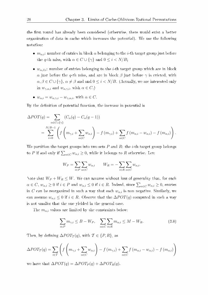
28 Chapter 3. Limits of Cache-Oblivious Rational Permutations
the rst round has already been considered (otherwise, there would exist a better
organization of data in cache which increases the potential). We use the following
notation:
• mα,i: number of entries in block α belonging to the i-th target group just before
the q-th miss, with α ∈ C ∪ γ and 0 ≤ i < N/B;
• wα,β,i: number of entries belonging to the i-th target group which are in block
α just before the q-th miss, and are in block β just before γ is evicted, with
α, β ∈ C ∪γ, α 6= β and and 0 ≤ i < N/B. (Actually, we are interested only
in wγ,α,i and wα,γ,i, with α ∈ C.)
• wα,i = wα,γ,i − wγ,α,i, with α ∈ C.
By the denition of potential function, the increase in potential is
∆POT (q) =∑
α∈C∪γ
(Cα(q)− Cα(q − 1))
=
N/B−1∑i=0
(f
(mγ,i +
∑α∈C
wα,i
)− f (mγ,i) +
∑α∈C
f (mα,i − wα,i)− f (mα,i)
).
We partition the target groups into two sets P and R: the i-th target group belongs
to P if and only if∑
α∈C wα,i ≥ 0, while it belongs to R otherwise. Let:
WP =∑i∈P
∑α∈C
wα,i WR = −∑i∈R
∑α∈C
wα,i.
Note that WP + WR ≤ W . We can assume without loss of generality that, for each
α ∈ C, wα,i ≥ 0 if i ∈ P and wα,i ≤ 0 if i ∈ R. Indeed, since∑
α∈C wα,i ≥ 0, entries
in C can be reorganized in such a way that each wα,i is non negative. Similarly, we
can assume wα,i ≤ 0 if i ∈ R. Observe that the ∆POT (q) computed in such a way
is not smaller that the one yielded in the general case.
The mα,i values are limited by the constraints below:∑i∈P
mγ,i ≤ B −WP ,∑α∈C
∑i∈R
mα,i ≤M −WR. (3.8)
Then, by dening ∆POTT (q), with T ∈ P,R, as
∆POTT (q) =∑i∈T
(f
(mγ,i +
∑α∈C
wα,i
)− f (mγ,i) +
∑α∈C
f (mα,i − wα,i)− f (mα,i)
)
we have that ∆POT (q) = ∆POTP (q) + ∆POTR(q).

3.2. Lower bounds 29
When i ∈ P , we have wα,i ≥ 0 and, by Lemma A.1, f (mα,i − wα,i)− f (mα,i) ≤−f (wα,i). Then,
∆POTP (q) ≤∑i∈P
[f
(mγ,i +
∑α∈C
wα,i
)− f (mγ,i)−
∑α∈C
f (wα,i)
].
By Inequalities 3.8 and Corollary A.4, an upper bound on ∆POTP (q) is obtained by
plugging mγ,i = (B −WP )/|P | and wα,i = WP/(|P ||C|) into the previous equation:
∆POTP (q) ≤ B logB
|P |− (B −WP ) log
B −WP
|P |−WP log
WP
|P ||C|
≤ (B −WP ) logB
B −WP
+WP logB|C|WP
≤ B +WP logM
WP
, (3.9)
since |C| < M/B.
When i ∈ R, we have wα,i ≤ 0 and, by Lemma A.1, f(mγ,i +
∑α∈C wα,i
)−
f (mγ,i) ≤ −∑
α∈C f (−wα,i). Therefore, we have:
∆POTR(q) ≤∑i∈R
∑α∈C
[f (mα,i − wα,i)− f (mα,i)− f (−wα,i)] .
By Lemma A.3 an upper bound on ∆POTR(q) is obtained by setting mα,i = (M −WR)/(|R||C|) and wα,i = −WR/(|R||C|). Then:
∆POTR(q) ≤M logM
|R||C|− (M −WR) log
M −WR
|R||C|−WR log
WR
|R||C|
≤ (M −WR) log
(1 +
WR
M −WR
)+WR log
M
WR
≤ WR logeM
WR
, (3.10)
since (1 + 1/x)x ≤ e if x ≥ 1.
By Equations 3.10 and 3.9, and the fact that WR + WP ≤ W , we derive the
following upper bound:
∆POT (q) ≤ B +WP logM
WP
+WR logeM
WR
≤ B +W log2eM
W.
Corollary 3.2. The increase in the potential function due to the q-th miss, with

30 Chapter 3. Limits of Cache-Oblivious Rational Permutations
1 ≤ q ≤ N/B, is upper bounded by 2B log 2eMB
.
Proof. When a block γ is fetched into the cache, at most 2B entries are exchanged be-
tween γ and the other blocks residing in cache. The corollary follows from Lemma 3.1
by setting W = 2B.
The following theorem restats the lower bound proved in [Cor93b, Theorem 2.23].
Theorem 3.3. Let Σ be an innite set of permutations which contains at most
one n-permutation for each n ∈ N. An algorithm which performs any rational N-
permutation ΠσN dened by an n-permutation σ ∈ Σ requires
Ω
(NζΣ(logB,N)
B log(1 +M/B)+N
B+ 1
)(3.11)
misses on an IC(M,B), for each value of M and B. 5
Proof. The Ω (N/B + 1) lower bound is straightforward because the input and output
vectors are distinct. The rst term of Equation 3.11 follows from Corollary 3.2 and
Equations 3.6 since
QΣ(N,M,B)∑q=1
∆POT (q) ≥ POT (QΣ(N,M,B))− POT (0)
2B log2eM
BQΣ(N,M,B) ≥ NζΣ(logB,N),
which yields
QΣ(N,M,B) ≥ NζΣ(logB,N)
2B log 2eMB
.
An obvious lower bound on the work complexity of an algorithm performing
rational permutations is Ω (N) since N entries have to be moved from the input
vector V to the output vector U . Moreover, this work complexity is attained by
the naïve algorithm which reads V sequentially and moves each entry V [i] directly
into U [Πσ−1
N (i)] (we remind that Πσ−1
N is the inverse of ΠσN), but this algorithm is
not cache-optimal. We wonder whether there is a cache-optimal IC algorithm whose
5Note that the lower bound given in [Cor93b] is Ω(N maxζΣ(logM,N),ζΣ(logB,N)
B log(M/B) + NB + 1
), but
it easy to see that it is asymptotically equivalent to Equation 3.11.

3.2. Lower bounds 31
work complexity is Θ (N) for each value of IC parameters. The following theorem
states that such an algorithm cannot exist.
Theorem 3.4. Let Σ be an innite set of permutations which contains at most one
n-permutation for each n ∈ N. Consider an algorithm which performs any rational
N-permutation ΠσN dened by an n-permutation σ ∈ Σ and whose cache complexity
is
QΣ(N,M,B) ∈ Θ
(NζΣ(logB,N)
B log(1 +M/B)+N
B+ 1
),
on an IC(M,B), for each value of M and B. Then its work complexity is
WΣ(N,M,B) ∈ Ω
(NζΣ(logB,N)
log(1 +M/B)+N
)(3.12)
when M/B > b, for a suitable constant b > 1.
Proof. If ζΣ(logB,N) ≤ log(1 + M/B), Equation 3.12 becomes the Ω (N) lower
bound. Suppose ζΣ(logB,N) > log(1 + M/B), and let c and d be two suitable
constants such that
cNζΣ(logB,N)
B log(1 +M/B)≤ QΣ(N,M,B) ≤ d
NζΣ(logB,N)
B log(1 +M/B). (3.13)
Denote with Q′Σ(N,M,B) the number of misses each of which increases the potential
by at least (B/2d) log(1 + M/B). We claim that Q′Σ(N,M,B) = Θ (QΣ(N,M,B)).
Let ∆POT be the upper bound given in Corollary 3.2 on the increase in the potential
function due to a miss, and let ∆POT1 = (B/2d) log(1 +M/B). Then,
POT (Q)−POT (0) ≤
≤ (QΣ(N,M,B)−Q′Σ(N,M,B)) ∆POT1 +Q′Σ(N,M,B)∆POT
≤ QΣ(N,M,B)∆POT1 +Q′Σ(N,M,B)∆POT
From Equations 3.6 and Inequality 3.13, we derive
Q′Σ(N,M,B)
(2B log
(2eM
B
))≥ NζΣ(logB,N)− dNζΣ(logB,N)
2d,
which implies
Q′Σ(N,M,B) ∈ Ω
(NζΣ(logB,N)
B log(1 +M/B)
).
Let q be a miss which increases the potential by at least ∆POT1, and let γ be the

32 Chapter 3. Limits of Cache-Oblivious Rational Permutations
block fetched into the cache in the q-th miss. By Lemma 3.1, if at most W entries
are exchanged between γ and the other blocks resident in cache with γ, the potential
increases by at most (B+W log(2eM/W )). IfM/B ≥ b for a suitable constant b > 1
and W < B/4d, then (B + W log(2eM/W )) < ∆POT1, which is a contradiction.
Then W = Θ (B). Since an IC operation moves only a constant number of words
between blocks, there are at least Ω (B) operations per miss. The theorem follows.
Corollary 3.5. Let Σ be an innite set of permutations which contains at most one
n-permutation for each n ∈ N. Each rational N-permutation ΠσN , dened by an
n-permutation σ ∈ Σ, can be performed by an optimal cache-aware algorithm with
work complexity
W (N,M,B) ∈ Θ
(Nζ(logB, σ)
log(1 +M/B)+N
),
and cache complexity
Q(N,M,B) ∈ Θ
(Nζ(logB, σ)
B log(1 +M/B)+N
B+ 1
),
on an IC(M,B), for each value of M and B.
Proof. An optimal algorithm for performing a rational permutation ΠσN in the Par-
allel Disk model [VS94] with p disks is given in [Cor93a]. By setting p = 1, this
algorithm translates automatically into an EM algorithm; then, by removing all I/O
operations, the algorithm becomes a cache-aware IC algorithm. Clearly, the number
of block transfers performed by the optimal o-line policy of the IC model cannot be
bigger than the number of disk accesses performed in the Parallel Disk model with
p = 1. This cache-aware algorithm is composed of ζ(logB, σ)/(B log(1 + M/B))
phases, each of which requires Θ (N) work and Θ (N/B) misses. By Theorems 3.3
and 3.4, this algorithm exhibits optimal cache and work complexities on an IC(M,B),
for each value of M and B.
Corollary 3.6. Matrix transposition and bit-reversal can be performed by an optimal
cache-aware algorithm with work complexity
W (N,M,B) ∈ Θ
(N log minB,N/B
log(1 +M/B)+N
),

3.3. Cache-oblivious algorithm for rational permutations 33
and cache complexity6
Q(N,M,B) ∈ Θ
(N log minB,N/BB log(1 +M/B)
+N
B+ 1
), (3.14)
on an IC(M,B), for each value of M and B.
Proof. The statement follows by Corollary 3.5 and Equations 3.3 and 3.4.
3.3 Cache-oblivious algorithm for rational permuta-
tions
In this section we propose an optimal cache-oblivious algorithm which performs each
rational permutation ΠσN on a vector V of N = 2n entries, where σ denotes an n-
permutation. It incurs Θ (N/B) misses and requires Θ (N) work on an IC(M,B)
that satises the tall-cache assumption. We also describe an ecient cache-oblivious
algorithm for computing all the values ΠσN(i), with 0 ≤ i < N , since the computation
of any such value cannot be considered as an elementary operation.
3.3.1 Computing the values of a rational permutation
Let N = 2n and let ΠσN be the rational permutation dened by the n-permutation σ.
In this subsection we describe an algorithm which computes a vector P of N entries,
where P [i] = ΠσN(i) for each i, with 0 ≤ i < N . The algorithm derives Πσ
N(i) from
ΠσN(i − 1) (note that Πσ
N(0) = 0 for each σ), comparing the binary representations
of i and i− 1.
Specically, the algorithm uses four vectors:
• S where S[j] = σ(j) for each j, with 0 ≤ j < n;
• I where I[j] = σ−1(j) for each j, with 0 ≤ j < n;
• P where, at the end of the algorithm, P [i] = ΠσN(i) for each i, with 0 ≤ i < N ;
• A where A[j] stores the j-th bit of the binary representation of the current
index i, with 0 ≤ j < n and 0 ≤ i < N (A[0] is the LSB).
6 In [AV88] a lower bound on the I/O complexity of matrix transposition in the EM model is
provided, which is Ω(N log minM,
√N,N/B
B log(1+M/B) + NB + 1
). This is also a valid lower bound on the cache
complexity of matrix transposition in the IC model, and coincides with Equation 3.14.

34 Chapter 3. Limits of Cache-Oblivious Rational Permutations
INPUT: a vector S of n entries which represents the n-permutation σ;OUTPUT: a vector P of N entries, with N = 2n, where P [i] = Πσ
N (i) for eachi, with 0 ≤ i < N ;
1: Compute I from S through Mergesort;2: Set all entries of A to 0;3: P [0]← 0;4: N ← 2n;5: for i = 1 to N − 1 do
6: P [i]← P [i− 1];7: j ← 0;8: while A[j] = 1 do9: A[j]← 0; // The j-th bit of i is set to 0
10: P [i]← P [i]− 2I[j]; // The I[j]-th bit of P [i] is set to 0
11: j ← j + 1;12: A[j]← 1; // The j-th bit of i is set to 1
13: P [i]← P [i] + 2I[j]; // The I[j]-th bit of P [i] is set to 1
Figure 3.1: Cache-oblivious algorithm for computing the values of a bit-permutationσ.
More succinct data structures can be adopted, but we maintain the ones above for
the sake of simplicity. The input of the algorithm is S (i.e., the bit-permutation
σ), while the output is P . Note that I can be computed from S through sorting.
The algorithm for computing P is divided into N − 1 stages: in the i-th stage, with
0 < i < N , the algorithm adds 1 (modulo N) to the binary representation of i − 1
stored in A, and derives P [i] from P [i− 1] according to the dierences between the
binary representations of i and i− 1. The pseudocode for the algorithm is reported
in Figure 3.1. Note that the algorithm is cache-oblivious and based on the binary
counter [CLRS01].
Theorem 3.7. The work and cache complexities of the algorithm in Figure 3.1 are:
W (N,M,B) ∈ Θ (N) , (3.15)
Q(N,M,B) ∈ Θ
(N
B
)(3.16)
on an IC(M,B), for each value of M and B such that M/B ≥ 4.
Proof. The vector I can be eciently computed through Mergesort with work com-
plexity o (N) and cache complexity o(N/B) [BF03].
In order to bound the cache complexity of the for loop (Steps 5-13), we describe a
particular replacement policy for the cache and compute the cache complexity using
this policy: since the IC model adopts an optimal o-line replacement policy, the
actual cache complexity cannot be larger than the one achieved by the policy we

3.3. Cache-oblivious algorithm for rational permutations 35
describe. We suppose the cache to have at least four lines, and we associate the
vectors I, P and A with three distinct cache lines: that is, there is exactly one cache
line for all the constituent blocks of each vector. The fourth line is used for support
variables. Since the entries of P are required in sequential order, each constituent
block of P is fetched only once into the line associated with P . Therefore, the number
of misses due to P is Θ (N/B).
Let αi be the memory block which contains entries A[iB], . . . , A[(i + 1)B − 1],
with 0 ≤ i < dn/Be. When an entry A[iB+ k], with 0 ≤ i < dn/Be and 1 ≤ k < B,
is required, the corresponding block αi is in cache since the previous required A's
entry was A[iB + k − 1], which also belongs to αi. On the other hand, when A[iB]
is referenced, block αi is not in cache and a miss occurs. Since A[j] ips N/2j times,
with 0 ≤ j < n, during the course of the algorithm [CLRS01], each block αi is fetched
into the cache N/2iB times. Therefore, the number of misses due to A is Θ(N/2B).
Since I[j] is read only after A[j] for each j, with 0 ≤ j < n, the upper bound for A is
also valid for I. Then, the number of misses due to I is Θ(N/2B). Equation 3.16 fol-
lows. Since there are Θ(B) operations for each block, Equation 3.15 follows as well.
3.3.2 Performing a rational permutation
In this subsection we present a cache-oblivious algorithm which performs any rational
permutation ΠσN on a vector V of N = 2n entries, where σ and V are given as input.
As usual, U denotes the output vector.
Before describing the algorithm, note that the recursive cache-oblivious algorithm
for matrix transposition described in [FLPR99] moves each entry of the input matrix
to the corresponding entry of the output matrix in an order based on the Z-Morton
layout [CLPT99]. This particular access pattern to V minimizes the cache complexity
of the algorithm under the tall-cache assumption. In the same fashion, our algorithm
rst derives an ecient access pattern for V from σ, and then it moves each entry
of V , in the order specied by the pattern, into the right entry of U . The access
pattern to V is dened by the n-permutation πσ: the i-th accessed element is V [j]
where j = ΠπσN (i) for each i, with 0 ≤ i < N . The n-permutation πσ is computed by
the algorithm in Figure 3.2.7
The algorithm for performing the rational permutation ΠσN on V is divided into
N steps: in the i-th step, the entry V [ΠπσN (i)] is moved into U [Π
(σ−1)N (Ππσ
N (i))], with
0 ≤ i < N . The pseudocode of the algorithm is given in Figure 3.3.
7For simplifying algorithms in Figures 3.2 and 3.3, we consider πσ, π−1σ , σ, σ−1 as vectors.

36 Chapter 3. Limits of Cache-Oblivious Rational Permutations
INPUT: an n-permutation σ;OUTPUT: the n-permutation πσ;1: Compute σ−1 from σ through Mergesort;2: i = 0; j = 0;3: while j < n do
4: if σ−1(i) ≥ i then π−1σ (j) = i; j = j + 1;
5: if σ(i) > i then π−1σ (j) = σ(i); j = j + 1;
6: i = i+ 1;7: Compute πσ from π−1
σ through Mergesort;
Figure 3.2: Cache-oblivious algorithm for computing the values of a bit-permutationπσ.
INPUT: an n-permutation σ, and a vector V of N = 2n entries;OUTPUT: a vector U of N entries, where U [Πσ−1
N (i)] = V [i] for each i, with0 ≤ i < N ;
1: Compute σ−1 from σ through Mergesort;2: Compute πσ through algorithm in Figure 3.2;
3: Compute the values of the bit-permutations ΠπσN and Π(σ−1)
N through algorithmin Figure 3.1;
4: for i = 0 to N − 1 do
5: U [Π(σ−1)N (Ππσ
N (i))] = V [ΠπσN (i)];
Figure 3.3: Cache-oblivious algorithm for performing a rational permutation ΠσN .
Let k be an arbitrary power of two, with 0 ≤ k ≤ N , and let l be an arbitrary
value with 0 ≤ l < N/k. Observe that, intuitively, the access pattern dened by
πσ guarantees that the k entries of V and U which are read and written during the
kl, . . . , k(l+ 1)− 1-st accesses, dier in at most (log k)/2 of the n− (log k)/2 MSBs.
This implies that Θ(√
k)cache lines of size Θ
(√k)suce to permute the k entries
incurring O(k/B +
√k)misses. An example of πσ is given later in Equation 3.17.
In order to prove the correctness and to evaluate the cache and work complexities
of the algorithm in Figure 3.3, we introduce the following two lemmas. The rst one
shows a property of πσ and that the algorithm in Figure 3.2 is well dened, while
the second lemma proves that πσ is actually an n-permutation.
Lemma 3.8. Let σ be an n-permutation, π−1σ (k) be the function computed in the
algorithm in Figure 3.2, and let %i,σ = π−1σ (k) : 0 ≤ k ≤ i + ζ(i + 1, σ). The
algorithm in Figure 3.2 is well dened and we have
%i,σ = 0, . . . , i ∪ IN (i+ 1, σ).
Proof. In order to prove the lemma, we show by induction on i, with 0 ≤ i < n− 1,
that at the end of the i-th iteration of the algorithm in Figure 3.2, we have j =

3.3. Cache-oblivious algorithm for rational permutations 37
i+ ζ(i+ 1, σ) + 1 (which also implies that %i,σ is well dened at the end of the i-th
iteration) and %i,σ = 0, . . . , i ∪ IN (i+ 1, σ). If i = 0 the claim is clearly true. Let
i > 0. Denote with j the value of j at the beginning of the i-th iteration, that is
j = (i − 1) + ζ(i, σ) + 1 by the inductive hypothesis. If i is assigned to π−1σ (j) in
Step 4, then i /∈ %i−1,σ: otherwise i ∈ %i−1,σ and, in particular, i ∈ IN (i, σ). If σ(i) is
assigned to π−1σ (j) or π−1
σ (j+1) in Step 5, then either σ(i) ∈ IN (i+1, σ)−IN (i, σ),
or σ(i) ∈ IN (i, σ). A simple case analysis shows that at the end of the i-th iteration
j = i+ ζ(i+ 1, σ) + 1 and %i,σ = 0, . . . , i ∪ IN (i+ 1, σ).
Since i < n in each iteration, σ(i) and σ−1(i) in Lines 4 and 5 do exist and,
therefore, the algorithm is well dened.
Lemma 3.9. Let σ be an n-permutation. Then the function πσ dened by the algo-
rithm in Figure 3.2 is an n-permutation.
Proof. We claim that π−1σ (hence πσ) is a permutation. Suppose, for the sake of
contradiction, that there are two values j′ and j′′, 0 ≤ j′ < j′′ < n such that
π−1σ (j′) = π−1
σ (j′′) = p. Clearly, p cannot be assigned to both π−1σ (j′) and π−1
σ (j′′) by
two steps of the same kind. Then, suppose that p is assigned to π−1σ (j′) in Step 4 and
to π−1σ (j′′) in Step 5: by the if statements in Steps 4 and 5, it follows that σ−1(p) ≥ p
and p > σ−1(p), respectively, but this is a contradiction. In the same fashion, it can
be proved that p cannot be assigned to π−1σ (j′) in Step 5 and to π−1
σ (j′′) in Step 4.
Therefore, π−1σ is a permutation since there are n values and no duplicates.
As example, consider the bit-permutation τn associated with the transposition of
a 2n/2 × 2n/2 matrix (Equation 3.1). Then π−1τn is so dened:
π−1τn (i) =
i2
if i even and 0 ≤ i < n
n2
+ i−12
if i odd and 0 ≤ i < n
. (3.17)
The access pattern dened by π−1τn coincides with the Z-Morton layout, that is, with
the access pattern used in the cache-oblivious algorithm for matrix transposition
given in [FLPR99]. According with Lemma 3.8 and Equation 3.2, it is easy to see
that:
%i,τn =
0, . . . , i ∪ n
2. . . n
2+ i if 0 ≤ i < n
2
0, . . . , n− 1 if n2≤ i < n− 1
.

38 Chapter 3. Limits of Cache-Oblivious Rational Permutations
Theorem 3.10. Let Σ be an innite set of permutations which contains at most one
n-permutation for each n ∈ N. The cache-oblivious algorithm in Figure 3.3 performs
each rational permutation ΠσN dened by an n-permutation σ ∈ Σ, and requires
W (N,M,B) ∈ Θ (N) (3.18)
work and
Q(N,M,B) ∈
O
(N
B
)if M
B≥ 21+ζ(logB,σ)
O
(NB
M
)if M
B< 21+ζ(logB,σ)
(3.19)
misses on an IC(M,B), for each value of M and B such that M/B > 4.
Proof. The correctness of the algorithm in Figure 3.3 follows from the fact that πσ
and ΠπσN are permutations.
We now analyze the work and cache complexities of the algorithm in Figure 3.3.
Recall that ζ(logB, σ) is the cardinality of OUT (j, σ) (or IN (j, σ) equivalently).
For simplifying the notation, we denote ζ(logB, σ) with ζ.
We now show that Steps 1, 2 and 3 require Θ (N) work and Θ (N/B) misses.
As argued in the proof of Theorem 3.7, the computation of the inverse of an n-
permutation requires o (N) work and o (N/B) misses. Thus, the computation of σ−1
and of the algorithm in Figure 3.2 (Steps 1-2) can be performed in o (N) operations
and o (N/B) misses. The computation of the values of ΠπσN and Π
(σ−1)N (Step 3)
requires linear work and Θ (N/B) misses (by Theorem 3.7).
We now upper bound the cache complexity of Steps 4-5, in which all the entries of
V are permuted into U . We distinguish between two cases: when the number M/B
of cache lines is bigger or smaller than 21+ζ . In both cases we analyze the number of
distinct blocks touched by a consecutive sequence (whose length is dierent in each
case) of accesses to V and U in the order dened by πσ. We show that, in the rst
case, Θ(2ζ)blocks of V and U are touched by B2ζ consecutive accesses while, in
the second case, O (M/B) blocks are touched by 2ϕM/(2B) accesses (ϕ is a suitable
value dened later).
Suppose MB≥ 21+ζ and partition the sequence of N accesses to V into N/(B2ζ)
segments. Let F i = ΠπσN (iB2ζ), . . . ,Ππσ
N ((i+ 1)B2ζ − 1), with 0 ≤ i < N/B2ζ , be
the set of the indices of the entries accessed in the i-th segment. By Lemma 3.8, the
binary representations of the values in F i dier on (logB + ζ) bit positions, and ζ
of these are the (logB)-incoming bit positions of σ, which are among the log(N/B)

3.4. Limits of cache-oblivious rational permutations 39
MSBs by denition. Then, the B2ζ entries of V with indices in F i are distributed
among 2ζ blocks. Moreover, in the (logB + ζ) bit positions there are also ζ (logB)-
outgoing bit positions of σ. Then, by the denition of outgoing bit position, the
B2ζ entries are permuted into 2ζ blocks of the output vector U . Since there are at
least 21+ζ cache lines, the permutation of entries indexed by the values in Fi requiresΘ(2ζ)misses, and the permutation of the whole vector V requires Θ (N/B) misses.
Suppose MB
< 21+ζ . Let ϕ be the maximum integer in [0, logB) such that
|OUT (logB, σ) ∩ OUT (ϕ, σ)| = log(M/2B), that is ϕ denotes the bigger bit po-
sition such that exactly log(M/2B) (logB)-incoming bit positions are permuted
into positions smaller than ϕ. Note that ϕ is well dened since |OUT (logB, σ)| =
ζ > log(M/(2B)). We use the previous argument, except for the segment length.
Specically, partition the sequence of N accesses to V into N/(2ϕM/(2B)) seg-
ments and let F i = ΠπσN (i2ϕM/(2B)), . . . ,Ππσ
N ((i+ 1)2ϕM/(2B)− 1, with 0 ≤ i <
N/(2ϕM/(2B)), be the set of the indices of the entries required in the i-th segment.
The binary representations of the values in F i dier on ϕ + log(M/(2B)) bit posi-
tions, and (log(M/2B)) of these are (logB)-incoming bit positions of σ. Then the
2ϕM/(2B) entries of V with indices in F i are distributed among M/(2B) blocks.
An argument similar to the one used above proves that these 2ϕM/(2B) entries are
permuted into at most M/(2B) blocks of the output vector U . Therefore, the per-
mutation steps requires O (N/2ϕ) = O (NB/M) misses, since ϕ ≥ log(M/(2B)), and
Equation 3.19 follows. The proof of Equation 3.18 is straightforward.
By Theorem 3.10 and the lower bounds on the work and cache complexities given
in Section 3.2, the cache-oblivious algorithm in Figure 3.3 is optimal when M/B ≥21+ζ(logB,σ). Since ζ(logB, σ) ≤ logB, the tall-cache assumption (i.e., M ≥ B2) is
sucient to guarantee cache and work optimality of the cache-oblivious algorithm for
each rational permutation. Recall that by Corollary 3.5, there exists a cache-aware
algorithm for performing rational permutations which exhibits optimal cache and
work complexities for all values of the IC parameters. In the next section, we will
show that an optimal cache-oblivious algorithm for all values of the IC parameters
cannot exist.
3.4 Limits of cache-oblivious rational permutations
Theorem 3.4 proves that the work complexity of a cache-optimal algorithm is ω(N)
when M/B ∈ o(2ζΣ(logB,N)
), and Θ (N) otherwise. Clearly, the work complexity of
a cache-oblivious algorithm is independent of the cache parameters (this is not the

40 Chapter 3. Limits of Cache-Oblivious Rational Permutations
case, in general, for cache complexity). Hence, a cache-oblivious algorithm cannot
have optimal work complexity for each value of M and B. One can wonder whether
there exists a cache-oblivious algorithm which is cache-optimal for each M and B,
regardless of the work complexity. In this section we will prove that such an algorithm
cannot exist. To this purpose we follow a similar approach to the one employed in
[BF03].
Let Σ be an innite set of permutations which contains at most one n-permutation
for each n ∈ N and let A be a cache-oblivious algorithm which performs any rational
N -permutation dened by an n-permutation σ ∈ Σ on a vector ofN entries. Consider
the two sequences of misses generated by the executions of A in two dierent ICs,
where one model satises a particular assumption we will dene, while the other
does not. We simulate these two executions in the EM model and obtain a new EM
algorithm solving the same problem as A. By adapting the argument described in
Subsection 3.2 to bound from below the number of disk accesses, we conclude that
A cannot be optimal in both ICs.
3.4.1 The simulation technique
In this subsection we describe a technique for obtaining an EM algorithm from two
executions of a cache-oblivious algorithm in two dierent IC models. The technique
is presented in a general form and is a formalization of the ad-hoc one employed in
[BF03] for proving the impossibility result for general permutations.
Consider two models C1=IC(M,B1) and C2 = IC(M,B2), where B1 < B2. For
convenience, we assume B2 to be a multiple of B1. Let A be a cache-oblivious
algorithm for an arbitrary problem and let Q1 and Q2 be its cache complexities
in the two models, respectively. We dene an algorithm A′ for EM(2M,B2) which
emulates in parallel the executions of A in both C1 and C2 and solves the same
problem as A.Let us regard the memory in EM(2M,B2) as partitioned into two contiguous
portions of size M each, which we refer to as M1 and M2, respectively. In turn,
portion M1 is subdivided into blocks of B1 words (which we call B1-rows), and
portionM2 is subdivided into blocks of B2 words (which we call B2-rows), so that
we can establish a one-to-one mapping between the cache lines of C1 and the B1-rows
ofM1, and a one-to-one mapping between the cache lines of C2 and the B2-rows of
M2. Algorithm A′ is organized so that its I/Os coincide (except for some slight
reordering) with the I/Os performed by A in C2, and occur exclusively between the
disk and M2. On the other hand, A′ executes all operations prescribed by A on

3.4. Limits of cache-oblivious rational permutations 41
data inM1.8 Since there are no I/Os betweenM1 and the disk, data are inserted
intoM1 by means of transfers of B1-rows betweenM1 andM2, which coincide with
the I/Os performed by A in C1.
Let us now see in detail how the execution of A′ in the EM(2M,B2) develops.
Initially all the words inM1 andM2 are empty, that is lled with NIL values, and the
EM disk contains the same data as the memory of C2 (or C1 indistinguishably) with
the same layout (a one-to-one relation between the B2-blocks of C2 and the B2-blocks
of the disk can be simply realized). Let oi be the i-th operation of A, i = 1 . . . h.
The execution of A in Ci, 1 ≤ i ≤ 2, can be seen as a sequence Li of operationsinterleaved with I/Os. Since operations in L1 and L2 are the same, we build a new
sequence L=Γ21Γ1
1o1 . . .Γ2jΓ
1joj . . .Γ
2hΓ
1hohΓ
2h+1Γ1
h+1. Each Γij, with 1 ≤ j ≤ h+ 1 and
1 ≤ i ≤ 2, is dened as follows:
• Γi1 is the sequence of I/Os that precede o1 in Li.
• Γij, 1 < j ≤ h, is the sequence of I/Os which are enclosed between oj−1 and oj
in Li.
• Γih+1 is the sequence of I/Os performed after oh in Li.
Note that a Γij can be empty. The length of L, denoted as |L|, is the sum of the
number h of operations and the size of all Γij, with 1 ≤ j ≤ h+ 1 and 1 ≤ i ≤ 2. Let
A′ be divided into |L| phases. The behavior of the j-th phase is determined by the
j-th entry lj of L:
1. lj is an operation: A′ executes the same operation inM1.
2. lj is an input of a B2-block (i.e., an input of L2): A′ fetches the same B2-block
from the disk into the B2-row ofM2 associated with the line used in C2.
3. lj is an input of a B1-block (i.e., an input of L1): let γ be such a B1-block and
γ′ be the B2-block containing γ. Since there is no prefetch in the IC model,
the next operation of A requires an entry in γ; thus γ′ must be in the cache of
C2, too. For this reason, we can assume that γ′ was, or has just been, fetched
into a B2-row ofM2. A′ copies γ in the right B1-row ofM1 and replaces the
copy of γ inM2 with B1 NIL values.
4. lj is an output of a B2-block (i.e., an output of L2): A′ moves the respective
B2-row ofM2 to the disk, replacing it with B2 NIL values.
8Note that the operations of A do not include I/Os since block transfers are automaticallycontrolled by the machine. Moreover, A's operations are the same no matter whether execution isin C1 or C2.

42 Chapter 3. Limits of Cache-Oblivious Rational Permutations
5. lj is an output of a B1-block (i.e., an output of L1): let γ be such a B1-block
and γ′ be the B2-block containing γ. If γ′ is still inM2, then A′ copies γ from
M1 into γ′ and replaces γ's row with B1 NIL values. The second possibility
(i.e., γ′ is not inM2) can be avoided since no operations are executed between
the evictions of γ′ and γ. If some operations were executed, both blocks γ and
γ′ would be kept in cache (and so inM1 andM2). Therefore, we can suppose
γ was removed just prior to the eviction of γ′.
It is easy to see that every operation of A can be executed by A′ in M1, since
there is a one to one relation between the cache lines of C1 and the rows ofM1 (except
for the B1-blocks whose evictions from cache were anticipated, see fth point). M2
is a quasi-mirror of C2, in the sense that it contains the same B2-blocks of C2 while
A is being executed, except for those sub B1-blocks which are also inM1. By rules
2 and 4, the I/O complexity of A′ is at most 2Q2 (note that a miss in the IC model
is equivalent to at most two I/Os in the EM model).
Let K = Q1B1/Q2; it is easy to see that K ≤ B2. Indeed, if K were greater
than B2, a replacement policy for C1 which requires Q2B2/B1 < Q1 misses would be
built from the execution of A in C2; but this is a contradiction since the replacement
policy of the IC model is optimal. A′ can be adjusted so that there are at most K
words exchanged between M1 and a B2-block in M2 before this block is removed
from the memory: it is sucient to insert some dummy I/Os. This increases the I/O
complexity of A′ from 2Q2 to at most 2Q2 + 2Q1B1/K = 4Q2 I/Os. In particular,
there are at most 2Q2 inputs and 2Q2 outputs of B2-blocks.
We dene the working set W(q) after q I/Os as the content of M1 plus the
words in the corresponding B2-blocks ofM2 that will be used by A′ (moved toM1)
before the B2-blocks are evicted. When A′ fetches a B2-block from the disk, we can
suppose that the at most K entries which will be moved betweenM1 and the block
are immediately included in the working set.
Note that the EM algorithm A′ could not be implementable in practice; however,
since we are interested in lower bounding its I/O complexity, this is not relevant ex-
cept in the case where the arguments used for bounding suppose the implementability
of A′. The argument used in the following section is based on a potential function
and does not require the algorithm to be implementable.
3.4.2 Impossibility result for rational permutations
In this subsection we prove that a cache-oblivious algorithm which performs the
rational permutations dened by a set Σ cannot be optimal for each value of the
cache parameters.

3.4. Limits of cache-oblivious rational permutations 43
Theorem 3.11. Let Σ be an innite set of permutations which contains at most one
n-permutation for each n ∈ N, and N range over 2n : ∃ an n-permutation σ ∈ Σ.Consider a cache-oblivious algorithm A which performs any rational N-permutation
dened by an n-permutation σ ∈ Σ. If there exists a function g(N) ≤ log(δN), with
δ ∈ (0, 1), such that ζΣ(g(N), N) ∈ ω(1), then A cannot be cache-optimal for each
value of the M and B parameters.
Proof. We begin by asserting that a lower bound on the cache complexity in the IC
model translates into a lower bound on the I/O complexity in the EM model, and
vice versa, since the IC model adopts an optimal o-line replacement policy [SCD02].
Moreover, the lower bound provided in Theorem 3.3 is tight since it can be matched
by an aware algorithm, as established in Corollary 3.5. Assume, for the sake of
contradiction, that A attains optimal cache complexity for each value of M and B.
In particular, consider two models C1=IC(M,B1) and C2 = IC(M,B2) where B2 is a
multiple of B1, and let Q1 and Q2 be the cache complexities of A in the two models,
respectively. We will show that B1 and B2 can be suitably chosen so that Q1 and
Q2 cannot be both optimal, thus reaching a contradiction. To achieve this goal, we
apply the simulation technique described in the previous subsection to A, and obtain
an algorithm A′ for the EM(2M,B2) solving the same problem as A. We then apply
an adaptation of Lemma 3.1 (which is based on a technical result given in [AV88] for
bounding from below the number of disk accesses of matrix transposition in the EM
model) to A′, and we prove the impossibility of the simultaneous optimality of A in
the two IC models. We denote with Q and QI the I/O complexity and the number
of inputs of B2-blocks, respectively, of A′; recall that Q ≤ 4Q2 and QI ≤ 2Q2.
As in Section 3.2, we dene the i-th target group, with 0 ≤ i < N/B2, to be
the set of entries that will ultimately be in the i-th B2-block of the output vector
(remember that it must be entirely in the disk at the end of A′). Let γ be a B2-block
of the disk or a B2-row ofM2; the togetherness rating of γ after q I/Os is dened
as:
Cγ(q) =
N/B2−1∑i=0
f(xγ,i),
where xγ,i denotes the number of entries in γ belonging to the i-th target group just
before the (q+ 1)-st I/O, and f is the convex function given in Equation 3.5. These
entries are not included in the working set W(q) and are not NIL symbol. We also

44 Chapter 3. Limits of Cache-Oblivious Rational Permutations
dene the togetherness rating for the working set W(q) as:
CW(q) =
N/B2−1∑i=0
f(si),
where si is the number of entries in the working set W(q) which belong to the i-th
target group just before the (q+ 1)-st I/O. The potential function of A′ after q I/Osis dened as:
POT (q) = CW(q) +∑γ∈disk
Cγ(q) +∑γ∈M2
Cγ(q).
At the beginning and at the end of the algorithm the above denition is equivalent
to the one given in Section 3.2. Then by Equations 3.6,
POT (0) = N log(B2/2ζΣ(logB2,N)), POT (Q) = N logB2.
Hence, POT (Q)− POT (0) = NζΣ(logB2, N).
We now bound the increase in the potential function due to the input of a B2-
block since the eviction of a block from the memory does not increase the potential.
Suppose that the q-th I/O is an input and a B2-block γ is fetched into a B2-row of
M2. Before the q-th input, the intersection between γ and the working setW(q−1)
was empty; after the input, at most K = Q1B1/Q2 entries of γ are inserted into
W(q − 1). We use the following notation:
• si: number of entries in the working set W(q − 1) belonging to the i-th target
group;
• ki: number of entries in γ belonging to the i-th target group just before the
q-th miss;
• wi: number of entries in the (at most) K words, inserted inW(q−1), belonging
to the i-th target group.
The si, ki and wi values are limited by the following constraints:
N/B2−1∑i=0
si ≤ 2M −K,N/B2−1∑i=0
ki ≤ B2,
N/B2−1∑i=0
wi ≤ K.

3.4. Limits of cache-oblivious rational permutations 45
The increase in the potential function due to the q-th miss (∆POT (q)) is:
∆POT (q) =
N/B2−1∑i=0
[f(si + wi) + f(ki − wi)− f(si)− f(ki)] .
By Lemma A.1, we have that f(ki − wi)− f(ki) ≤ −f(wi). Thus,
∆POT (q) ≤N/B2−1∑i=0
[f(si + wi)− f(si)− f(wi)] . (3.20)
According with Corollary A.4 an upper bound on ∆POT (q) is obtained by setting
si = (2M −K)/(N/B2) and wi = K/(N/B2) in Inequality 3.20:
∆POT (q) ≤N/B2−1∑i=0
[si log
si + wisi
+ wi logsi + wiwi
]≤ K log e+K log
2M
K= K log
2eM
K,
since (1 + 1/x)x ≤ e if x ≥ 1. Let C1 be a cache with more than 2ζΣ(logB1,N) lines,
while C2 be a cache with less than 2ζΣ(logB2,N) lines. By Theorem 3.3, cN/B1 ≤Q1 ≤ dN/B1 for two suitable positive constants c and d. Since the number of input
operations is QI ≤ 2Q2 (remember that the output of a block does not increase the
potential and that K = Q1B1/Q2), we have that
POT (Q)− POT (0) ≤QI∑q=1
∆POT (q) ≤ 2Q2K log2eM
K≤ 2dN log
2eMQ2
cN.
By recalling that POT (Q)− POT (0) = N log 2ζΣ(logB2,N),
N log 2ζΣ(logB2,N) ≤ 2dN log2eMQ2
cN.
Hence,
Q2 ∈ Ω
(N
2ζΣ(logB2,N)
2d
M
). (3.21)
By setting B2 = δ′M and M = 2g(N)/δ′, for a constant δ, with 0 < δ′ < δ, we have
ζΣ(logB2, N) = ζΣ(g(N), N) ∈ ω(1),

46 Chapter 3. Limits of Cache-Oblivious Rational Permutations
which yields (the asymptotic is on N)
Q2 ∈ ω(NζΣ(g(N), N)
M
).
However, by optimality of A and Theorem 3.3, Q2 must be Θ(N ζΣ(g(N),N)
M
)when
B2 = δ′M , which yields a contradiction.
Corollary 3.12. There cannot exists a cache-oblivious algorithm for matrix trans-
position or bit-reversal that yields optimality for all values of the IC parameters.
Proof. Matrix transposition and bit-reversal are examples of rational permutations
which, by Equation 3.3 and 3.4, satisfy the hypothesis of Theorem 3.11 by setting
g(N) = dlog√Ne. Thus, Theorem 3.11 implies that cache-oblivious algorithms for
matrix transposition or the bit-reversal of a vector cannot exhibit optimal cache
complexity for all values of the cache parameters.
Note that Theorem 3.11 do not rule out the existence of an optimal cache-
oblivious algorithm for some particular ranges of the cache parameters. Indeed by
Theorem 3.10, there exists an optimal cache-oblivious algorithm under the tall-cache
assumption.

Chapter 4
Network-Oblivious Algorithms
I'm totally, totally oblivious. Usually.
(Paul Hewitt)
As seen in Section 2.2, a number of parallel models aim at realizing an eciency/
portability/ design-complexity tradeo by capturing features common to most ma-
chines through a number of parameters. One parameter present in virtually all
models is the number of processors, and most models also exhibit parameters de-
scribing the time required to route certain communication patterns. Increasing the
number of parameters, from just a small constant to logarithmically many in the
number of processors (like in the D-BSP), can considerably increase the eectiveness
of the model with respect to realistic architectures, such as point-to-point networks,
as extensively discussed in [BPP07]. However, a price is paid in the increased com-
plexity of algorithm design necessary to gain greater eciency across a larger class
of machines.
It is natural to wonder whether, at least for some problems, algorithms can be
designed that, while independent of any machine/model parameters, are nevertheless
ecient for a wide range of such parameters. In other words, we are interested in
exploring the world of ecient network-oblivious algorithms, in the same spirit as
the exploration of ecient cache-oblivious algorithms proposed in [FLPR99].
Of course, the rst step is to develop a framework where the concept of network-
obliviousness and of algorithmic eciency are precisely dened. The framework we
propose is based on three models of computation, each with a dierent role, as briey
outlined next.
• Specication model. This model, denoted by M(n), is a set of n CPU/memory
nodes, called processing elements (PEs), computing in supersteps, and able to
exchange messages. Network-oblivious algorithms will be formulated in this
47

48 Chapter 4. Network-Oblivious Algorithms
model. The number of PEs is chosen by the algorithm designer exclusively as
a function of the input size n. (Reasonably, n reects the amount of parallelism
of the algorithm at hand).
• Evaluation model. This model, denoted by M(p,B), has two parameters: the
number of processors, p, and a block size, B, which models the xed payload
size of any message exchanged by two processors. As forM(n), the computation
is organized in supersteps. A cost function is dened, called the block degree of
a superstep, which, when summed over all supersteps of an algorithm, gives the
communication complexity of the algorithm. An M(n) algorithm will execute
on an M(p,B), with p ≤ n, by letting each M(p,B) processor carry out the
work of a pre-specied set of n/p PEs of M(n).
The quality of a network-oblivious algorithm A, with input size n, is dened
with respect to the communication complexity HA(n, p,B) of its execution on
M(p,B), by measuring how close HA(n, p,B) comes to the minimum communi-
cation complexity H∗(n, p,B) achievable by any M(p,B) algorithm solving the
same problem as A. Algorithm A is optimal if HA(n, p,B) = O (H∗(n, p,B)),
for a suitably large range of (p,B) values.
• Execution machine model. This model aims at describing the set of platforms
on which we expect the network-oblivious algorithm to be actually executed.
Technically, we adopt for this role the block-based variant of the Decompos-
able Bulk Synchronous Parallel model, D-BSP(P, g,B), [BPP07] described in
Section 2.2.1, where g and B are vectors of length logP .
Fortunately, as shown in the next section, for a wide and interesting class of
network-oblivious algorithms, optimality with respect to the M(p,B) model,
for suitable ranges of (p,B), translates into optimality with respect to the
D-BSP(p, g,B), for suitable ranges of g and B. It is this circumstance that
motivates the introduction of the evaluation model, as a tool to substantially
simplify the performance analysis of oblivious algorithms.
To help placing our network-oblivious framework in perspective, it may be useful
to compare it with the well established cache-oblivious framework [FLPR99]. In
the latter, the algorithm formulation model is the Random Access Machine; the
algorithm evaluation model is the Ideal Cache model IC(M,B), a machine with only
one level of cache of size M and line length B; and the machine execution model is
a machine with a hierarchy of caches, each with its own size and line length. In the
cache-oblivious context, the simplication in the analysis arises from the fact that,

4.1. The framework 49
under certain conditions, optimality on IC(M,B) for all values ofM and B translates
into optimality on multilevel hierarchies.
The structure of this chapter is as follows. In Section 4.1, we dene rigorously the
three models relevant to the framework and establish the key relations among them.
In Section 4.2, we illustrate the framework by deriving positive and negative results
on network-oblivious algorithms for key problems, such as matrix multiplication
and transposition, FFT, and sorting. We also show that matrix transposition does
not admit network-oblivious algorithms, for some range of parameters. The results
presented in this chapter were published in [BPPS07].
4.1 The framework
In this section, we introduce the models of computation for the formulation and
analysis of network-oblivious algorithms, and develop some key relations between
these models, which provide the justication for the framework.
Specication model. Let Π be a given computational problem and let n (for
simplicity, a power of two) be a suitable function of the input size. A network-
oblivious algorithm A for Π is designed for a complete network M(n) of n Processing
Elements (PEs), PE0, . . ., PEn−1, each consisting of a CPU and an unbounded local
memory. A consists of a sequence of labeled supersteps1, with labels in the integer
range [0, log n). For 0 ≤ i < log n and 0 ≤ j < n, in an i-superstep, PEj can perform
operations on locally held data, and send words of data only to any PEk whose index
k agrees with j in the i most signicant bits, that is, bj2i/nc ≤ k < bj2i/nc+ n/2i.
The superstep ends with a global synchronization.
Evaluation model. In order to analyze A's communication complexity on dier-
ent machines, we introduce the machine model M(p,B), where the parameters p and
B are positive integers (for simplicity, powers of two). M(p,B) is essentially an M(p)
with a communication cost function parameterized by B, whose processing elements
are called processors and denoted as pj, with 0 ≤ j < p, to distinguish them from
those of M(n). Words exchanged between two processors in a superstep can be en-
visioned as traveling within blocks of xed size B (in words). For each superstep we
dene the block-degree as the maximum number of blocks sent/received by a single
processor in that superstep. More formally, the block-degree of a superstep s where
1The results would hold even if, in the various models considered, supersteps were not explicitlylabeled. However, explicit labels can help reduce synchronization costs; they become crucial forecient simulation of algorithms on point-to-point networks, especially those of large diameter.

50 Chapter 4. Network-Oblivious Algorithms
processor pj sends wsjk words to pk, with 0 ≤ j, k < p, is dened as
hs(p,B) = max0≤j<p
max
(p−1∑k=0
dwsjk/Be,p−1∑k=0
dwskj/Be
).
The communication complexity of an algorithm is the sum of the block-degrees of
its supersteps. Hence, the model rewards batched over ne-grained communication.
The quantity hs = hs(p, 1) is also called the word-degree of superstep s. Clearly,
dhs/Be ≤ hs(p,B) ≤ hs. Although the network-oblivious framework is primarily
concerned with communication, we dene a cost function, called computation com-
plexity, which measures, in some sense, the degree of parallelism. The computation
complexity of an algorithm is the sum over all supersteps of the maximum number
of operations performed by a processor on locally held data during a superstep.
A network-oblivious algorithm A formulated for M(n) can be naturally executed
on an M(p,B) machine, for every 1 ≤ p ≤ n and for every B, by stipulating that
processor pj, with 0 ≤ j < p, of M(p,B) will carry out the operations of the n/p
consecutively numbered processing elements of M(n) starting with PE(n/p)j. Super-
steps with a label i < log p on M(n) become supersteps with the same label on
M(p,B); supersteps with label i ≥ log p become local computation. Let us number
the supersteps of A from 1 to S, where S is the number of supersteps executed by
the algorithm on M(p,B), and let hs(n, p,B) be the block-degree of the execution of
superstep s. The central quantity in our analysis is the communication complexity
HA(n, p,B) =S∑s=1
hs(n, p,B),
of A on an M(p,B), for varying p and B.
With regard to the computation complexity of a network-oblivious algorithm
for M(n), we observe that the simulation of a superstep s on M(p,B) requires
O ((n/p)(τ s + hs)) operations, where τ s is the maximum number of operations ex-
ecuted by a PE on locally held data and hs is the maximum number of words
sent/received by a PE (i.e, the word-degree on M(n, 1)); O ((n/p)hs) is the cost
of a naïve message dispatching. Without loss of generality we assume hs ∈ O (τ s),
that is, Ω (1) operations are performed for each sent or received message. We de-
note with TA(n, p,B) the computation complexity of a network-oblivious algorithm
A with input size n on M(p,B).
As a cache-oblivious algorithm ignores, hence cannot explicitly use, cache size
and line length, so does a network-oblivious algorithm ignore, hence cannot explicitly

4.1. The framework 51
use, the actual number of processors that will carry out the computation, and the
block size of the communication.
Denition 4.1. A network-oblivious algorithm A for a problem Π is optimal if for
every p and B, with 1 < p ≤ n and B ≥ 1, the execution of A on an M(p,B) machine
yields an algorithm with asymptotically minimum communication complexity among
all M(p,B) algorithms for Π.
Execution machine model. To substantiate the usefulness of the above deni-
tion, we now show that, under certain assumptions, an optimal network-oblivious
algorithm can run optimally on an wide class of parallel machines, whose underlying
interconnection network exhibits a hierarchical structure with respect to its band-
width characteristics. To model machines in this class, we use the block variant
of the Decomposable BSP (D-BSP) model described in Section 2.2.1, denoted as a
D-BSP(P, g,B), where g = (g0, g1, . . . glogP−1) and B = (B0, B1, . . . BlogP−1). Note
that a D-BSP(P, g,B) is essentially an M(P ) machine, where the communication
time of superstep s is dened to be hs(P,Bi)gi, where i is the label of the superstep
and hs(P,Bi) denotes the block-degree of the superstep.
In the reminder of this section, we show that an optimal network-oblivious algo-
rithm A translates into an optimal D-BSP algorithm under some reasonable assump-
tions on the communication pattern employed by the algorithm and on the machine
parameters. We begin with the following technical lemma.
Lemma 4.2. For m ≥ 1, let 〈X0, X1, . . . , Xm−1〉 and 〈Y0, Y1, . . . , Ym−1〉 be two arbi-
trary sequences of nonnegative integers, and let 〈f0, f1, . . . , fm−1〉 be a nonincreasing
sequence of nonnegative real values. If∑i
j=0 Xj ≤∑i
j=0 Yj, for every 0 ≤ i < m,
thenm−1∑j=0
Xjfj ≤m−1∑j=0
Yjfj.
Proof. By dening S−1 = 0 and Sj =∑j
i=0(Yi − Xi) ≥ 0, for 0 ≤ j ≤ m − 1, we
have:
m−1∑j=0
fj(Yj −Xj) =m−1∑j=0
fj(Sj − Sj−1) =m−1∑j=0
fjSj −m−1∑j=1
fjSj−1 ≥
≥m−1∑j=0
fjSj −m−1∑j=1
fj−1Sj−1 = fm−1Sm−1 ≥ 0.

52 Chapter 4. Network-Oblivious Algorithms
In the next denitions, we introduce some useful parameters and properties of
network-oblivious algorithms.
Denition 4.3. Given an algorithm A for M(n), we dene i-granularity bi, for
0 < i ≤ log n, the minimum number of words ever exchanged by two communicating
PEs in any superstep of the execution of A on an M(2i, 1).
In other words, when executing A on M(2i, 1), in any superstep, if pj sends any
words to pk, then it sends at least bi words to it.
Denition 4.4. Let α > 0 be constant. An algorithm A for M(n) is said to be
(α, P )-wise if, for any i with 1 < 2i ≤ P , we have
HA(n, 2i, 1) ≥ αn
2i
∑s∈Li
hs(n, n, 1).
where Li is the set of indices of the supersteps with labels j < i.
To put the above denition into perspective, we observe that an algorithm where
for each j-superstep and for every i > j there is always at least one segment of n/2i
consecutively numbered PEs each communicating the maximum amount of words
for that superstep to PEs outside the segment, is surely an (α, P )-wise algorithm.
However, (α, P )-wiseness holds even if the aforementioned communication scenario
is realized only in an average sense.
Many algorithms are likely to exhibit a good level of granularity and can be ar-
ranged to be (α, P )-wise. Indeed, this is the case for all network-oblivious algorithms
presented in this chapter. Quite interestingly, these algorithms achieve optimal per-
formance on D-BSP, as better established in the following theorem.
Theorem 4.5. Let A be an (α, P ∗)-wise optimal network-oblivious algorithm for a
problem Π with input size n, specied for the M(n) model, with i-granularity bi, for
0 ≤ i < logP ∗. Then, A exhibits asymptotically optimal communication time when
executed on any D-BSP(P, g,B), with P ≤ P ∗ and Bi ≤ blogP , for 0 ≤ i < logP .
Proof. Let DA(i), with 0 ≤ i < logP , be the sum of block-degrees of all i-supersteps
when A is executed on D-BSP(P, g,B). From the hypothesis on the granularity of A,we have that the minimum amount of words ever exchanged by two communicating
PEs in any superstep is at least blogP ≥ Bi, for every 0 ≤ i < logP . Hence,
DA(i) ≤ 2n
P
∑s∈Li+1\Li
hs(n, n, 1)
Bi
, ∀0 ≤ i < logP.

4.1. The framework 53
Since A is (α, P ∗)-wise, we have that
HA(n, 2i, Bi) ≥HA(n, 2i, 1)
Bi
≥ α∑s∈Li
n
2ihs(n, n, 1)
Bi
≥ αi−1∑j=0
n
2iBi
∑s∈Lj+1\Lj
hs(n, n, 1) ≥ α
2
i−1∑j=0
P
2iDA(j)
Bj
Bi
.
By denition, the overall communication time of A on D-BSP(P, g,B) is H =∑logP−1j=0 DA(j)gj. Suppose A′ were an asymptotically faster D-BSP(P, g,B) algo-
rithm for Π. Then, for every constant ε > 0 and suciently large input size n, A′
would exhibit communication time H ′ < εH, so that, with obvious notation,
logP−1∑j=0
DA′(j)gj < ε
logP−1∑j=0
DA(j)gj.
The above relation can be rewritten as
logP−1∑j=0
DA′(j)BjgjBj
< ε
logP−1∑j=0
DA(j)BjgjBj
.
Recalling from Section 2.2.1 that the ratios gi/Bi are assumed to be non-increasing,
we can apply Lemma 4.2, with m = logP , fj = gj/Bj, Xj = εDA(j)Bj, and
Yj = DA′(j)Bj, to show that there exists an i ≤ logP such that
i−1∑j=0
DA′(j)Bj < εi−1∑j=0
DA(j)Bj.
Now, we can naturally interpret A′ as an M(2i, Bi) algorithm, whose communication
complexity satises
HA′(n, 2i, Bi) ≤
i−1∑j=0
P
2iDA′(j)
Bj
Bi
< εi−1∑j=0
P
2iDA(j)
Bj
Bi
≤ 2ε
αHA(n, 2i, Bi),
which is a contradiction, since 2ε/α is an arbitrary value and, by denition, A is
asymptotically optimal for M(2i, Bi). (Note that in the above inequalities we used
the fact that the Bj's are powers of two and non-increasing.)
As a nal remark, observe that by setting all block sizes equal to 1, the above
framework can be specialized to the case where the block transfer feature is not

54 Chapter 4. Network-Oblivious Algorithms
accounted for.
4.2 Algorithms for key problems
In this section we present optimal network-oblivious algorithms for a number of rel-
evant computational problems, namely matrix multiplication, matrix transposition,
FFT and sorting. In some cases, optimality requires additional constraints on the
relative values of some machine and input parameters and, in one case, we will prove
that these constraints are necessary to obtain network-oblivious optimality. The cor-
rectness of the algorithms will not be discussed since they are straightforward (e.g.,
matrix transposition) or already proved in the literature (e.g., matrix multiplication,
FFT, sorting).
This section is organized as follows. In Sections 4.2.1 and 4.2.2 we describe
the network-oblivious algorithms for matrix multiplication and transposition, re-
spectively. In Section 4.2.3 we show that there cannot exist a network-oblivious
algorithm for matrix transposition which is optimal for all values of the parameters.
Then, in Sections 4.2.4 and 4.2.5, we provide network-oblivious algorithms for FFT
and sorting, respectively.
4.2.1 Matrix multiplication
The n-MM problem requires to multiply two n× n matrices using only semiring op-
erations [Ker70]. In this section we propose two network-oblivious algorithms which
both yield optimal communication complexities, while they exhibit dierent memory
requirements. We rst establish lower bounds on the communication complexity of
any M(p,B) algorithm for this problem.
Theorem 4.6. Let A be any algorithm solving the n-MM problem on an M(p,B),
with 1 < p ≤ n2 and B ≥ 1. If initially the inputs are evenly distributed among the
p processors, then the communication complexity of the algorithm is
Ω
(n2
Bp2/3
). (4.1)
Moreover, if each processor cannot contain more than O (n2/p) entries of the input
and output matrices in each superstep, then the communication complexity is:
Ω
(n2
B√p
). (4.2)

4.2. Algorithms for key problems 55
Proof. The lower bound in Equation 4.2 is a consequence of [ITT04, Theorem 4.1]:
this theorem requires the local memory of each processor to be upper bounded by
O (n2/p), thus making no distinction between the local memory used for storing input
and output entries (and their possible copies) and the local memory used for others
data structures (e.g., the space required for simulating network-oblivious algorithms
on an M(p,B)). Nevertheless, the proof remains valid when imposing the O (n2/p)
limit only to the number of input and output entries in a processor.
Irony et al. [ITT04, Lemma 5.1] provided the lower bound in Equation 4.1 as-
suming a O(n2/p2/3
)upper bound on the local memory of each processor. However,
the same lower bound was proved, without the assumption, in [Pie95, CFSV95] for
M(p, 1).
Next, we describe an optimal network-oblivious algorithm, which we name N-MM
(Network-oblivious Matrix Multiplication), for the n-MM problem whose communica-
tion complexity matches the lower bound in Equation 4.1. The algorithm is specied
on M(n2). Let A, B and C denote the two input matrices and the output matrix,
respectively, and suppose that their entries are evenly distributed among the PEs.
For 0 ≤ i, j < n, we denote with P (i, j) the processing element PEin+j of M(n2),
and require that such a PE holds A[i, j], B[i, j], and C[i, j]. We denote a quadrant
of matrix E (E ∈ A,B,C) with Ehk, with h, k ∈ 0, 1.2 Let ` ∈ 0, 1, deneMhk` = Ah` ·B`k, whence Chk = Mhk0+Mhk1. The algorithm is based on the following
simple recursive strategy, where we denote withm and q the number of rows/columns
of the (sub)matrices involved and the number of assigned PEs, respectively (initially,
m = n and q = n2).
1. Regard the q PEs as partitioned into eight segments Shk`, with h, k, ` ∈ 0, 1,of q/8 PEs each. Replicate and distribute the inputs so that the entries of Ah`
and B`k are evenly spread among the PEs in Shk`. (Note that each Shk` is an
M(q/8) machine.)
2. For h, k, ` ∈ 0, 1 in parallel, compute recursively the product Mhk` within
Shk`.
3. For h, k ∈ 0, 1 in parallel, Mhk0 and Mhk1 are evenly distributed among PEs
in Shk0 and Shk1 is such a way that Mhk0[i, j] and Mhk1[i, j] are contained by
the same PE for each 0 ≤ i, j < m/2.
2Quadrants are the following: E00 (top-left), E01 (top-right), E10 (bottom-left), E11 (bottom-right).

56 Chapter 4. Network-Oblivious Algorithms
4. For 0 ≤ i, j < m in parallel, C[i, j] is computed by adding Mhk0[i, j] and
Mhk1[i, j].
The recurrence stops when only one PE is assigned to a subproblem (i.e., q = 1).
The parameter m decreases by a factor two, while the number q of PEs assigned to
each subproblem by a factor eight. Since, at the beginning of the algorithm, m = n
and q = n2, each PE, in the base case, must multiply sequentially two matrices of
size n1/3 × n1/3.
Theorem 4.7. The communication and computation complexities of the network-
oblivious algorithm N-MM for the n-MM problem, when executed on an M(p,B)
machine, with 1 < p ≤ n2 and 1 ≤ B ≤ n2/p, are
HN−MM(n, p,B) ∈ Θ
(n2
Bp2/3
), (4.3)
TN−MM(n, p,B) ∈ Θ
(n3
p
), (4.4)
which are optimal for all values of p and B in the specied ranges. The algorithm
requires a O(n2/3
)memory blow-up per processor.
Proof. Consider the execution of a recursive call with input size m and q assigned
PEs, and let r be the number of M(p,B) processors that simulate the q PEs (r ≤ q).
Let H(m, r) be the communication complexity of a recursive call to N-MM. Since
there is no communication when the q PEs are simulated by the same processor, it
follows that (for simplicity B and q are omitted from H(m, r)):
H(m, r) ≤
H(m
2,r
8
)+O
(m2
Br
)if r > 1
0 if r ≤ 1
which yields
H(m, r) ∈ O(
m2
Br2/3
).
Equation 4.3 follows by setting m = n, q = n2 and r = p; its optimality descends
from Theorem 4.6. Let T (m, q, r) denote the computation complexity of a recursive
call to N-MM, where m, q and r are dened as in H(m, r); clearly, TN−MM(n, p,B) =

4.2. Algorithms for key problems 57
T (n, n2, p). T (m, q, r) is upper bounded by the following recurrence:
T (m, q, r) ≤
T(m
2,q
8,r
8
)+O
(m2
r
)if r > 1
8T(m
2,q
8, 1)
+O(m2)
if r ≤ 1 and q > 1
O(m3)
if r ≤ 1 and q ≤ 1
which yields
T (m, q, r) ∈ O(m3
r
).
Note that the inequality q > 1 in the recurrence is equivalent to m > n1/3. Each PE
in M(n2) requires S(n, n2) space, where S(m, q) denotes the space required by a PE
for executing a recursive call of N-MM with parameters m and q. S(m, q) is upper
bounded by the following equation:
S(m, q) ≤
S(m
2,q
8
)+O
(m2
q
)if q > 1
O(m2)
if q ≤ 1
from which it follows that
S(m, q) ∈ O(m2
q2/3
).
Each M(p,B) processor requires O (S(n, n2)n2/p) space, hence the algorithm incurs
a O(n2/3
)memory blow-up.
N-MM solves the eight recursive subproblems Mhk` in parallel: the parallelism
decreases the communication complexity of the algorithm, but it causes a non-
constant memory blow-up. By solving the subproblems in two rounds, during which
only four subproblems are solved in parallel, it is possible to dene a network-
oblivious algorithm with a constant memory blow-up, but communication complexity
Θ(n2/B
√p). The algorithm, which we denote with SN-MM (Succinct Network-
oblivious Matrix Multiplication), is optimal for Theorem 4.6 because each processor
holds at most Θ (n2/p) entries of the input and output matrices.
SN-MM is dened in M(n2) and computes C+A ·B, where A, B and C are three
n × n matrices. Suppose the three matrices to be distributes among the PEs as in
N-MM. As before, we refer to a quadrant of a matrix E (E ∈ A,B,C) as Ehk,with h, k ∈ 0, 1. The algorithm is based on the following simple recursive strategy,

58 Chapter 4. Network-Oblivious Algorithms
where parameters m and q are employed with the same meaning as before (initially,
m = n and q = n2):
1. Regard the q PEs as partitioned into four segments Shk, with h, k ∈ 0, 1, ofq/4 PEs each. (Note that each Shk is an M(q/4) machine.)
2. Redistribute the inputs so that the entries of Ah0 and B0h are evenly spread
among the PEs in Shh, and the entries of Ah1 and B1k evenly spread among
the PEs in Shk, for h, k ∈ 0, 1 and h 6= k.
3. For h, k ∈ 0, 1 and h 6= k in parallel, compute recursively Chh + Ah0 · B0h
within Shh. and Chk + Ah1 ·B1k within Shk.
4. Redistribute the inputs so that the entries of Ah1 and B1h are evenly spread
among the PEs in Shh, and the entries of Ah0 and B0k evenly spread among
the PEs in Shk, for h, k ∈ 0, 1 and h 6= k.
5. For h, k ∈ 0, 1 and h 6= k in parallel, compute recursively Chh + Ah1 · B1h
within Shh. and Chk + Ah0 ·B0k within Shk.
6. Redistribute the inputs so that the entries of Ahk and Bhk are evenly spread
among the PEs in Shk, for h, k ∈ 0, 1.
Since the subproblem size m2 and the number of assigned PEs decrease by a factor
four, it follows that in each recursive call with input size m there are m2 PEs. The
recurrence stops when a subproblem is solved by an unique PE, that is, when the
subproblem size is one: in this case, C + A · B is computed locally. SN-MM is
equivalent to the D-BSP algorithm given in Theorem 2.5 when P = n2, where P
denotes the number of D-BSP processors.
Theorem 4.8. The communication and computation complexities of the network-
oblivious algorithm SN-MM for the n-MM problem, when executed on an M(p,B)
machine, with 1 < p ≤ n2 and 1 ≤ B ≤ n2/p, are
HSN−MM(n, p,B) ∈ Θ
(n2
B√p
), (4.5)
TSN−MM(n, p,B) ∈ Θ
(n3
p
), (4.6)
which are optimal for all values of p and B in the specied ranges. The algorithm
incurs a O (log n) memory blow-up per processor.

4.2. Algorithms for key problems 59
Proof. Observe that any recursive call with input size m is solved by q = m2 PEs.
Let H(m, r) denote the communication complexity of a recursive call to SN-MM,
where m and r denote the input size and the number of assigned M(p,B) processors,
respectively. It follows that:
H(m, r) ≤
2H(m
2,r
4
)+O
(m2
Br
)if r > 1
0 if r ≤ 1
which yields
H(m, r) ∈ O(m2
B√r
).
Equation 4.5 follows because HSN−MM(n, p,B) = H(n, p). Let T (m, r) denote the
computation complexity of a recursive call to SN-MM, where m and r are dened as
usual.
T (m, r) ≤
2T(m
2,r
4
)+O
(m2
r
)if r > 1
8T(m
2, 1)
+O(m2)
if r ≤ 1 and m > 1
O (1) if r ≤ 1 and m ≤ 1
which yields
T (m, r) ∈ O(m3
q
).
Since the input and output matrices are evenly distributed among the PEs and their
entries are not replicated, the optimality of the communication complexity follows
from Equation 4.2 of Theorem 4.6. The memory blow-up is due to the machine stack
size of each PE, which has size O (log n) because each PE performs log n recursive
and nested calls to SN-MM. The execution of SN-MM on an M(p,B) exhibits the
same memory blow-up.
The next lemma states that SN-MM can be transformed into an iterative network-
oblivious algorithm without increasing its communication and computation complex-
ities.
Lemma 4.9. The network-oblivious algorithm SN-MM can be transformed into an
iterative network-oblivious algorithm. Its communication and computation complex-
ities on an M(p,B), with 1 < p ≤ n2 and 1 ≤ B ≤ n2/p, do not change, while no

60 Chapter 4. Network-Oblivious Algorithms
additional space for stack is required.
Proof. We show that the stack of a PE can be simulated by a constant number of
words. In a recursive call of SN-MM, each PE must know the size of the subproblem
and on which submatrices of A, B and C is working. However, the size can be
represented in a global variable m which is divided by two before a recursive call and
multiplied by two when a call nishes. Furthermore, the submatrices of A, B and C
on which a PE is working is uniquely determined by the size of the subproblem and
the PE's ID.
Thus, the stack is required only for storing the return address of a recursive call.
However, in SN-MM there are only two possible return addresses (Lines 3 and 5),
thus only one bit is sucient for storing them. Since there are at most log n nested
calls, it follows that the machine stack can be simulated by log n bits. Since on an
M(n2) there are n2 PEs, we can suppose the log n bits to be stored in a constant
number of words.
The additional memory due to the stack is also required by the network-oblivious
algorithms for FFT and sorting, but we will not discus this issue further since the
approach used for SN-MM applies to these algorithms as well.
We now apply Theorem 4.5 to show that N-MM and SN-MM are both optimal
in a D-BSP. (Remember that the D-BSP model assumes that both the Bi's and the
ratios gi/Bi are non increasing.)
Corollary 4.10. SN-MM and N-MM perform optimally on a D-BSP(P, g,B) where
1 < P ≤ n2 and 1 ≤ Bi ≤ n2/P for each 0 ≤ i < logP . In particular, the
communication time of SN-MM is:
DSN−MM(n, P, g,B) ∈ Θ
(n2
P
logP−1∑i=0
2i/2giBi
). (4.7)
Proof. Consider an i-superstep s of SN-MM or N-MM and let hs be the maximum
number of words sent or received by a PE. It is easy to see that there exists a set
of q = n2/2i consecutive numbered PEs where almost all PEs in the rst half of q/2
PEs send Θ (hs) messages to PEs in the second half. Hence, the word-degree of s
on an M(2j, 1), with j > i, is Θ (hsn2/2j) and algorithms SN-MM and N-MM are
(α, n2)-wise, for a suitable constant α. Since the i-granularity of SN-MM is Θ (n2/2i),
the corollary follows from Theorem 4.5. Equation 4.7 can be derived as Equation 2.3
in Theorem 2.5.

4.2. Algorithms for key problems 61
In conclusion, N-MM attains a better communication time than SN-MM, however
the former requires a O(n2/3
)memory blow-up. If a constant memory blow-up is
desired, the (iterative) SN-MM algorithm must be used; however, communication
time will increase [ITT04]. For the optimality of SN-MM in the D-BSP, it follows
that Equation 4.7 provides also a lower bound on the communication time for the
n-MM problem on a D-BSP(P,g,B) where Bi ≤ n2/P for each i, with 0 ≤ i < logP .
4.2.2 Matrix transposition
The n-MT problem consists of transposing an n × n matrix. To completely specify
the problem in the parallel setting, we require that, initially (resp., nally), the
entries of the matrix are evenly distributed among the available PEs according to a
row-major (resp., column-major) ordering. While the problem is trivially solved on
any M(p, 1) machine, as we will see, it becomes harder for larger block sizes. The
following theorem establishes a lower bound on the communication complexity of the
n-MT problem.
Theorem 4.11. Let A be an algorithm solving the n-MT problem on an M(p,B),
with 1 < p ≤ n2 and 1 ≤ B ≤ n2/p. The communication complexity of the algorithm
is
Ω
(n2
Bp
(1 +
log(min(n2/p), p)log(1 + n2/(Bp))
)).
Proof. We use an argument similar to the one employed in [AV88] (see also Sec-
tion 3.2) to bound from below the I/O complexity of transposition in the EM model.
For 0 ≤ i < p, we dene the i-th target group as the set of entries that will be in
processor pi at the end of the algorithm. Let H be the communication complexity
of the algorithm and H ′ ≤ Hp be the overall number of blocks exchanged by the
processors during the entire execution. Let us index the blocks communicated among
the processors from 1 to H ′, so that the indices assigned to blocks communicated
in one superstep are smaller than those assigned to blocks communicated in any
subsequent superstep. For 0 ≤ t ≤ H ′, dene xi,j(t) as the number of entries of the
i-th target group held by pj after block t has been communicated (xi,j(0) reects the
initial condition). We dene the potential of A after the block of index t has been
communicated as
POT(t) =
p−1∑i=0
p−1∑j=0
f(xi,j(t)),
where f(x) = x log x, for x > 0, and f(0) = 0. We now bound POT(0): if p ≥ n, each
processor contains one entry for each of n2/p target groups, hence POT (0) = 0; if
p < n, each processor contains n/p rows of the input matrix, hence it contains n2/p2

62 Chapter 4. Network-Oblivious Algorithms
entries of p target groups and POT (0) ≤ n2 log(n2/p2). It follows that POT(0) ≤n2 log(d(n/p)2e) for each 1 ≤ p ≤ n2; clearly, POT(H ′) = n2 log(n2/p). By reasoning
as in [AV88], it can be shown that, for a suitable constant c > 0, the block of index
t increases the potential by the quantity3
POT(t)− POT(t− 1) ≤ cB log
(1 +
n2
Bp
)def
= ∇POT. (4.8)
Therefore,
p ·H · ∇POT ≥ POT(H ′)− POT(0) = n2 log
(n2
p
)− n2 log
(⌈(n
p
)2⌉)
,
and the theorem follows.
We now describe a network-oblivious algorithm, named N-MT, for the n-MT
problem on M(n2). For a nonnegative integer i, let B(i) denote the binary repre-
sentation of i, and let B−1(·) be such that B−1(B(i)) = i. Given two binary strings
u = (ud−1 . . . u0) and v = (vd−1 . . . v0) we let u ./ v denote their bitwise interleaving,
that is, u ./ v = ud−1vd−1 . . . u0v0. Let A be the n × n input matrix and let P (i, j)
denote the processing element PEin+j, which initially holds A[i, j] and at the end
will hold AT [i, j], with 0 ≤ i, j < n. The algorithm consists of a 1-superstep followed
by a 0-superstep.
1. For 0 ≤ i, j < n, P (i, j) sends A[i, j] to the PEq, where q = B−1(B(i) ./ B(j));
2. For 0 ≤ q < n2, if the PEq has received entry A[i, j] in the previous substep,
then it forwards it to P (j, i).
We observe that the rst superstep rearranges matrix entries according the Z-Morton
permutation dened in [CLPT02]. The correctness of the algorithm is evident. The
communication complexity of the above algorithm, whose correctness is immediate,
is established in the following theorem.
Theorem 4.12. The communication and computation complexities of the network-
oblivious algorithm N-MT when executed on an M(p,B) machine, with 1 < p ≤ n2
3Equation 4.8 can, loosely speaking, be derived from Lemma 3.1 by setting M = n2/p andW = B.

4.2. Algorithms for key problems 63
and 1 ≤ B ≤ n/√p, are
HN−MT(n, p,B) ∈ Θ
(n2
Bp
)(4.9)
TN−MT(n, p,B) ∈ Θ
(n2
p
)(4.10)
respectively, which are optimal for the specied ranges of p and B.
Proof. Suppose B, p and n are powers of two and 1 ≤ B ≤ n/√p. Let Bk, with
0 ≤ k < n2/B, denotes the k-th segment of B consecutive PEs of M(n2), that
is, PEkB . . . PE(k+1)B−1. Note that PEs within the same Bk hold A's entries that
are in the same row and belong to B dierent columns whose addresses dier in
the logB least signicant bits, assuming B ≤ n/√p. Hence, in the rst superstep
PEs in every Bk send their entries to PEs belonging to a segment of size at most
B2/2 ≤ n2/p. In the second superstep, P (j, i) receives an entry from PEq, where
q = B−1(B(i) ./ B(j)); thus PEs in every Bk receives all their data from PEs be-
longing to a segment of size B2. Therefore, since a segment of B2 ≤ 2n2/p PEs is
contained in at most four M(p,B) processors, the block-degree of the communication
involved in each superstep is O (n2/(Bp)). Optimality follows from Theorem 4.11.
If B, n or p are not powers of two, then the algorithm and the proof work by con-
sidering the nearest powers of two (which are a multiplicative factor two apart).
The following corollary is a consequence of Theorems 4.5 and 4.12:
Corollary 4.13. The network-oblivious algorithm N-MT performs optimally on a
D-BSP(P, g,B) where 1 < P ≤ n2 and 1 ≤ Bi ≤ n/√p, for each 0 ≤ i < logP .
Proof. It is easy to see that in each i-superstep, with i ∈ 0, 1 and for each
i < j < log n2, there exists a segment of Θ (n2/2j) consecutive numbered PEs
each communicating the maximum amount of words (that is, O (n2/2j)) for that
superstep to PEs outside the segment; then the algorithm is (α, n2)-wise. From the
proof of Theorem 4.12, it follows that two communicating processors of M(2i, B),
with 0 < i ≤ log n2 and B ≤ n/2i/2, exchange at least Ω (B) words; hence, the
i-granularity is Θ(n/2i/2
). The corollary follows from Theorem 4.5.
4.2.3 Impossibility result for matrix transposition
The constraint on B in the above theorem is what we call small-block assumption and
is reminiscent of the tall-cache assumption made in the context of cache-oblivious

64 Chapter 4. Network-Oblivious Algorithms
algorithms [FLPR99]. We will now prove that, under reasonable constraints, the
small-block assumption is necessary to achieve network-oblivious optimality for the
n-MT problem, just as the tall-cache assumption was shown to be necessary to
achieve cache-oblivious optimality for n-MT (see Section 3). We say that an M(p,B)
algorithm is full if in each of its supersteps all processors send/receive the same
number of blocks, within constants, and each block contains Θ (B) data words.
Theorem 4.14. There cannot exist a network-oblivious algorithm A for the n-MT
problem such that, for every 1 < p ≤ n2 and 1 ≤ B ≤ n2/p, its execution on M(p,B)
yields a full algorithm whose communication complexity matches the one stated in
Theorem 4.11.
Proof. Assume that such a network-oblivious algorithm A exists, and let H1 and H2
be the communication complexities of A when executed on M(p1, B1) and M(p2, B2),
with p1 > p2. Since the two executions are full by hypothesis, and every data commu-
nicated in the M(p2, B2) execution must be also communicated in the M(p1, B1) exe-
cution, we must have that B1p1H1 ∈ Ω (B2p2H2), whence B1p1H1/(B2p2H2) ∈ Ω (1)
(the asymptotic is with reference to n). Now, let us choose p1 = n2/2, B1 = 1,
p2 = Θ (n2−ε), for an arbitrary constant 0 < ε < 1, and B2 ∈ Θ (n2/p2). Then, by
Theorem 4.11 we have that (B1p1H1)/(B2p2H2) ∈ Θ (1/ log n) = o (1), a contradic-
tion.
Next, we prove that the n-MT lower bound can always be matched by parameter-
aware full algorithms, hence the impossibility stated above stems from requiring
network-obliviousness.
Theorem 4.15. For every 1 < p ≤ n2 and 1 ≤ B ≤ n2/p, there exists a full M(p,B)
algorithm for the n-MT problem whose communication complexity matches the one
stated in Theorem 4.11.
Proof. The algorithm is obtained by suitably parallelizing the strategy of [AV88]
employed for solving the n-MT problem in the EM model. In each processor, the
Θ (n2/p) records are partitioned into dierent target groups; each group in the de-
composition is called a target subgroup. Before the start of the algorithm, the size of
each target subgroup is d(n/p)2e.The algorithm uses a merging procedure. The records in the same target subgroup
remain together throughout the course of the algorithm. In each superstep, target
subgroups are merged and become bigger. The algorithm terminates when each
target subgroup is complete, that is, when each target subgroup has size Θ (n2/p). In
each superstep, which has block-degree Θ (n2/(Bp)), the size of each target subgroup

4.2. Algorithms for key problems 65
increases by the multiplicative factor n2/(Bp). Hence, the number i of supersteps
required by the algorithm is given by:⌈n
p
⌉2(n2
Bp
)i≥ n2
p.
Since the block-degree of each round is Θ (n2/(Bp)) the theorem follows.
As an example, consider the case when B = Θ (n2/p). The algorithm divides the
input matrix into n2/k2 submatrices of size k × k, with k = minn, n2/p. Since
the matrix is distributed according with a row-major layout, each processor contains
dn/pe rows of a submatrix. Then, in parallel, processors assigned to a submatrix
transpose it by means of a binary merge; after that, each processor completely con-
tains one target group and, in the nal superstep, the target groups are moved in
the right nal destinations. It is easy to see that the algorithm requires
Θ
(log
k
dn/pe
)= Θ
(log minn2/p, p
)supersteps, whose block-degree is O (1).
4.2.4 FFT
The n-FFT problem consists of computing an n-input FFT dag. The following
theorem establishes a lower bound on the communication complexity of any M(p,B)
algorithm for this problem.
Theorem 4.16. Let A be any algorithm solving the n-FFT problem on an M(p,B)
with 1 < p ≤ n and B ≥ 1. If the word-degree of each superstep is Θ (n/p), then the
communication complexity of A is:
Ω
(n
Bp
log n
log(1 + n/p)
).
Proof. Observe that the or of n bits can be computed by means of the FFT dag.
Hence, the lower bound given in [Goo99, Theorem 4.2] on the number of supersteps
for computing the or of n bits on an M(p, 1) translates into a lower bound for the
n-FFT problem. Since the word-degree of each superstep is Θ (n/p), the theorem
follows.
The network-oblivious n-FFT algorithm, called N-FFT, on M(n) exploits the

66 Chapter 4. Network-Oblivious Algorithms
well-known recursive decomposition of the dag into two sets of√n-input FFT sub-
dags, with each set containing√n such dags [ACS87]. Inputs are initially distributed
one per PE in such a way that the inputs of the j-th subdag in the rst set are assigned
to the j-th segment of√n consecutively numbered PEs (i.e., an M(
√n) machine).
The outputs of the rst set of subdags are permuted to become the inputs of the
second set, where the permutation pattern is equivalent to the matrix transposition
of an√n×√n matrix (i.e.,
√n-MT); thus, the permutation can be performed with
the network-oblivious algorithm N-MT. We have:
Theorem 4.17. The communication and computation complexities of the network-
oblivious algorithm N-FFT, when executed on an M(p,B) machine, with 1 < p ≤ n
and 1 ≤ B ≤√n/p, are
HN−FFT(n, p,B) ∈ Θ
(n
Bp
log n
log(1 + n/p)
)(4.11)
TN−FFT(n, p,B) ∈ Θ
(n
plog n
)(4.12)
which are optimal for the specied ranges of p and B.
Proof. When the algorithm is run on an M(p,B) machine with p ≤√n, each subdag
is computed locally by a single processor, and in this case, we must account only for
the transposition step, which entails each processor sending and receiving O (n/(Bp))
blocks for Theorem 4.12.
Each recursive call of the algorithm with input size m is solved by m PEs, and
let r be the number of M(p,B) processors that simulate these PEs. Since in each
recursive level, the m PEs perform a matrix transposition, each processor has block-
degree O (m/(Br)) and the communication complexity of the recursive call, H(m, r)
obeys the subsequent recurrence (for simplicity B is omitted from H(m, r)):
H(m, r) ≤
2H
(√m,
r√m
)+O
( mBr
)if r > 1
0 if r ≤ 1
which yields
H(m, r) ∈ O(m
Br
logm
log(1 +m/r)
).
Equation 4.11 is obtained by settingm = n and r = p, and its optimality follows from
Theorem 4.16 since the word-degree of an M(p,B) processor is Θ (n/p). The com-
putation complexity, T (m, r), of the recursive call is instead given by the following

4.2. Algorithms for key problems 67
recurrence:
T (m, r) ≤
2T
(√m,
r√n
)+O
(mr
)if r > 1
2√mT
(√m, 1
)+O (m) if r ≤ 1 and m > 1
O (1) if r ≤ 1 and m ≤ 1
and we have
T (m, r) ∈ O(mr
logm)
Equation 4.12 is obtained by setting m = n and r = p, and is optimal because an
n-input FFT dag contains Θ (n log n) nodes.
Observe that the small-block assumption is needed to guarantee an O (n/(Bp))
communication complexity for the matrix transposition problem within the algo-
rithm. It is an interesting open problem to determine to what extent such an
assumption is really needed in the n-FFT case. A similar question regarding the
tall-cache assumption is open in the realm of cache-obliviousness.
The following theorem is a consequence of Theorems 4.5 and 4.17:
Corollary 4.18. The network-oblivious algorithm N-FFT performs optimally on a
D-BSP(P, g,B) where 1 < P ≤ n and 1 ≤ Bi ≤√n/p for each 0 ≤ i < logP .
Proof. Note that N-FFT's communications are due to matrix transposition. By
Corollary 4.13, it follows that N-FFT is (α, n)-wise4 and its i-granularity is Θ(n/2i/2
).
The corollary follows from Theorem 4.5.
4.2.5 Sorting
The n-Sort problem consists of sorting n keys. We require that the inputs are evenly
distributed among the PEs, and that, at the end, the keys held by the i-th PE are
all smaller than or equal to those held by the j-th PE, for every j > i. The following
theorem establishes a lower bound on the communication complexity of any M(p,B)
algorithm for this problem.
Theorem 4.19. Let A be an algorithm solving the n-Sort problem on an M(p,B),
with 1 < p ≤ n and B ≥ 1. If the word-degree of each superstep is Θ (n/p), then the
4The algorithm given by the concatenation of supersteps of (α, P )-wise algorithms is still (α, P )-wise.

68 Chapter 4. Network-Oblivious Algorithms
communication complexity of A is:
Ω
(n
Bp
log n
log(1 + n/p)
)
Proof. The theorem follows by dividing by B the lower bound for M(p, 1) given in
[Goo99]
We now describe a network-oblivious algorithm, called N-Sort, for n-Sort based
on a recursive version of the Columnsort algorithm as described in [Lei92]. We
regard both the n keys and the PEs of M(n) as arranged on a s × r matrix with
s = n1/3 and r = n2/3. The algorithm consists of seven phases numbered from 1 to
7. During Phases 1, 3, 5 and 7 the keys in each row are sorted recursively (except
in Phase 5 where adjacent rows are sorted in reverse order) by r consecutive PEs
(i.e., an M(n2/3) machine). During Phase 2 (resp., 4) a transposition (resp., reverse
transposition) of the s×r matrix is performed maintaining the s×r shape. In Phase
6 two steps of odd-even transposition sort are applied to each column.
Theorem 4.20. The communication and computation complexities of the network-
oblivious algorithm N-Sort, when executed on an M(p,B) machine with 1 < p ≤ n
and 1 ≤ B ≤√n/p are
HN−Sort(n, p,B) ∈ O
(n
Bp
(log n
log(1 + n/p)
)log3/2 4),
TN−Sort(n, p,B) ∈ O(n
Bp(log n)log3/2 4
).
The communication complexity is optimal when p ≤ n1−ε, for any constant ε with
0 < ε < 1.
Proof. The transposition performed in Phases 2 and 4 can be implemented by sep-
arately transposing in parallel the r/s submatrices of size s × s and then suitably
permuting the rows of the s × r matrix. By employing the network-oblivious al-
gorithm described in Subsection 4.2.2 for each submatrix and by using the stated
upper bound on B, the transposition of the s × r matrix has communication com-
plexity Θ (n/(Bp)). The stated communication and computation complexities of the
entire algorithm is obtained by solving the following recurrences, where H(m, τ) and
T (m, τ) are the communication and computation complexities of a recursive call with

4.2. Algorithms for key problems 69
input size m and solved by τ processors of M(p,B).
H(m, τ) ≤
4H(m2/3,
τ
m1/3
)+O
( mBτ
)if τ > 1
0 if v ≤ 1
∈ O
(m
Bτ
(logm
log(1 +m/τ)
)log3/2 4)
T (m, τ) ≤
4T(m2/3,
τ
m1/3
)+O
(mτ
)if τ > 1
4m1/3T(m2/3, 1
)+O (m) if m > 1 and τ > 1
O (1) if m ≤ 1 and τ ≤ 1
∈ O(mr
(logm)log3/2 4).
Observe that when executed on an M(p,B) the network-oblivious algorithm N -Sort
has the property that the word-degree of each superstep is Θ (n/p), hence the lower
bound given in Theorem 4.19 applies to it.
We conjecture that a similar result can be obtained by adapting other known sorting
algorithms such as, for example, the one in [Goo99].
The following theorem is a consequence of Theorems 4.5 and 4.20:
Corollary 4.21. The above network-oblivious algorithm for the n-Sort problem per-
forms optimally on a D-BSP(P, g,B) where P ≤ n1−ε and 1 ≤ Bi ≤√n/p for each
0 ≤ i < logP .
Proof. The proof is similar to the one for Corollary 4.18.

70 Chapter 4. Network-Oblivious Algorithms

Chapter 5
Network-Oblivious Algorithms for
the Gaussian Elimination Paradigm
An algorithm must be seen to be believed.
(Donald Knuth)
In Chapter 4, we described the network-oblivious framework and proposed some
network-oblivious algorithms for fundamental problems, namely matrix multipli-
cation and transposition, FFT and sorting. In this chapter we present network-
oblivious algorithms which implement the Gaussian Elimination Paradigm (GEP)
[CR06]. Prominent problems, like Floyd-Warshall's all-pairs shortest paths, Gaus-
sian Elimination without pivoting, LU decomposition, and matrix multiplication,
can be solved through this paradigm.
Specically, we propose three algorithms, named N-GEP, εN-GEP and PN-GEP,
which exploit the recursive structure of parallel and cache-oblivious implementations
of GEP introduced in [CR07, CR08]. The three algorithms exhibit optimal commu-
nication and computation complexities in the evaluation model for suitable values
of the processor number and communication block size. Furthermore, N-GEP yields
optimal performance also in the D-BSP model for certain ranges of the parameters.
The rest of the chapter is organized as follows. In Section 5.1, we dene GEP
and the two parallel implementations given in [CR07, CR08]. Then, in Section 5.2,
we describe and analyze our network-oblivious algorithms.
71

72 Chapter 5. Network-Oblivious Algorithms for GEP
INPUT: n × n matrix x, function f : S × S × S × S → S, set Σf of triplets〈i, j, k〉, with 0 ≤ i, j, k < n.
OUTPUT: transformation of x dened by f and Σf .1: for k ← 0 to n− 1 do2: for i← 0 to n− 1 do3: for j ← 0 to n− 1 do
4: if 〈i, j, k〉 ∈ Σf then
5: x[i, j]← f(x[i, j], x[i, k], x[k, j], x[k, k]);
Figure 5.1: Gaussian Elimination Paradigm (GEP).
5.1 Preliminaries
5.1.1 Denition of GEP
Let x be an n × n matrix with entries chosen from an arbitrary domain S, and let
f : S ×S ×S ×S → S be an arbitrary function, which we call update function. (For
simplicity, we assume n to be a power of two). By Gaussian Elimination Paradigm
(GEP) we refer to the computation dened by the pseudocode in Figure 5.1 where
the algorithm modies x by applying a given set of updates, denoted by 〈i, j, k〉, withi, j, k ∈ [0, n), of the form
x[i, j]← f(x[i, j], x[i, k], x[k, j], x[k, k]).
We let Σf denote the set of such updates that the algorithm needs to perform. We
refer to Σf and n as update set and input size, respectively. We suppose that the
inclusion check in Line 4 and function f are computed in constant time and without
indirect addressing (for avoiding unexpected cache misses). Observe that an entry
of x can be used many times and assume dierent values as a result of updates in
Σf ; by changing the order of the updates, the result of the GEP computation can
be dierent.
As noted in [CR06] and illustrated in Figure 5.2, many problems can be solved
using a GEP computation, including Floyd-Warshall's all-pairs shortest paths, Gaus-
sian Elimination without pivoting, LU decomposition and matrix multiplication.
The following denition will be used for proving the correctness of the network-
oblivious algorithms for GEP. We say a GEP computation is commutative if its
update function f exhibits the following property: for each y, u1, v1, w1, u2, v2, and
w2 in S,
f(f(y, u1, v1, w1), u2, v2, w2) = f(f(y, u2, v2, w2), u1, v1, w1).

5.1. Preliminaries 73
INPUT: n× n matrix x.OUTPUT: Gaussian elimination without pivoting of x.1: for k ← 0 to n− 1 do
2: for i← 0 to n− 1 do
3: for j ← 0 to n− 1 do
4: if (k < n− 2) ∧ (k < i < n− 1) ∧ (k < j) then5: x[i, j]← x[i, j]− x[i,k]
x[k,k]x[k, j];
INPUT: n× n matrix x.OUTPUT: the all-pairs shortest paths of an n-node graph dened by the adja-
cency matrix x.1: for k ← 0 to n− 1 do
2: for i← 0 to n− 1 do
3: for j ← 0 to n− 1 do
4: x[i, j]← x[i, j] min(x[i, k] + x[k, j]);
INPUT: three n× n matrices a, b and c.OUTPUT: c← a · b.1: for k ← 0 to n− 1 do
2: for i← 0 to n− 1 do3: for j ← 0 to n− 1 do4: c[i, j]← c[i, j] + a[i, k] · b[k, j];Remark: the computation requires three matrices, but it can easily transformedinto a GEP computation by considering one n×n matrix that encloses a, b and c.
Figure 5.2: Examples of GEP computations. From the top: Gaussian eliminationwithout pivoting, Floyd-Warshall's all-pairs shortest paths, matrix multiplicationwith semiring operations.
Not all GEP computations are commutative, however all of the instances of GEP for
the aforementioned problems can be easily seen to be commutative.
5.1.2 Previous cache-oblivious and parallel implementations
of GEP
Chowdhury and Ramachandran proposed in [CR06] a cache-oblivious recursive im-
plementation of the GEP paradigm, called I-GEP. It executes updates in Σf in an
order dierent than the one induced by the algorithm in Figure 5.1. Updates are
performed in I-GEP in such a way to minimize cache misses and increase implicit par-
allelism. In general, changing the order of the updates may yield a dierent output,
thus aecting the correctness of the computation. In fact, it is proved in [Cho07] that
I-GEP produces the correct output under certain conditions on f and Σf , which are
met by all notable instances mentioned before. Furthermore, in [CR07] the authors
present an extension of I-GEP, referred to as C-GEP, which implements correctly any

74 Chapter 5. Network-Oblivious Algorithms for GEP
instance of GEP with no degradation in performance. We refer to the original papers
for more details. The cache complexity of I-GEP is O(n3/B
√M)when executed on
an IC(M,B), which is optimal in the worst-case because it matches the lower bound
on the cache complexity of matrix multiplication with semiring operations [HK81].
Below we describe two parallel implementations of I-GEP, which will be at the
base of our network-oblivious algorithms. These two versions, which we name PI-
GEP1 and PI-GEP2, have been presented in [CR07] and [CR08], respectively, for
a CREW (concurrent read, exclusive write) shared-memory model composed of p
processors and one level of cache, which can be either shared or distributed1. In
this model parallel tasks are assigned to processors by a scheduler. PI-GEP1 and
PI-GEP2 correctly solve any GEP computation that is correctly solved by I-GEP,
however they can be extended to fully generality by adopting the ideas in C-GEP.
PI-GEP1, whose pseudocode is reproduced in Appendix B for completeness,
adopts a recursive strategy where in each call it performs all updates
x[i, j]← f(x[i, j], x[i, k], x[k, j], x[k, k])
such that 〈i, j, k〉 ∈ Σf ∩ (I × J ×K), where I = [i0, i1], J = [j0, j1] and K = [k0, k1]
are suitable subranges of the full range [0, n). For the initial call we have I = J =
K = [0, n). Put in another way, we can imagine that the four operands of f come,
in order, from the following four submatrices of x, some of which may coincide:
• X ≡ x[I, J ],
• U ≡ x[I,K],
• V ≡ x[K, J ],
• W ≡ x[K,K].
There are four dierent types of recursive calls which are implemented by four re-
cursive functions A, B, C and D. Function A is invoked when I = J = K, hence
X = U = V = W . Function B is invoked when I = K and I ∩ J = ∅, hence X = V
and U = W . Function C is invoked when J = K and I ∩ J = ∅, hence X = U and
V = W . Finally, function D is invoked when both I ∩K = ∅ and J ∩K = ∅, henceall four submatrices X,U, V and W are disjoint. The initial call is A(x, n). In each
function, the four submatrices X,U, V and W are partitioned into four quadrants
referred to, with obvious notation, as Xi,j, Ui,j, Vi,j and Wi,j, with 0 ≤ i, j ≤ 1, and
the eight subproblems they induce are solved recursively (some in parallel). It is
1In [CR07] and [CR08], both PI-GEP1 and PI-GEP2 are referred to as I-GEP.

5.2. Network-Oblivious Algorithms 75
Algorithm(constraints onp and B)
Communicationcomplexity on
M(p,B)
Computationcomplexity on
M(p,B)
Optimality onM(p,B)
Optimality onD-BSP(P,g,B)
N-GEP(p ≤ n2/ log2 n,
B ≥ 1)O(
n2
B√p + n log2 n
)Θ(n3
p
) whenp ≤ n2/ log4 n
and B ≤n/(√p log2 n)
whenP ≤ n/ log nand Bi ∈O(n2i/2
P logn
)εN-GEP with ε
arbitraryconstant in
(0, 1)(p ≤ n2/ log4/3,B ≤ (n/
√p)1+ε)
O(
n2
B√p log2 logn
log(n2/p)
)O(n3
p log2 lognlog(n2/p)
)when p ≤ n2−δ,
andB ≤ (n/
√p)1+ε,
with δ anarbitrary
constant in (0, 2)
open problem
PN-GEP(p ≤ n2,B ≥ 1)
O(
n2
B√p + n
)Θ(n3
p
)when p ≤ n2 and
B ≤ n/√p no
Figure 5.3: Properties of network-oblivious algorithms described in this chapter.
shown in [CR07] that the algorithm requires O(n3/p+ n log2 n
)computational time
and the number of misses performed by all p processors matches the O(n3/B
√M)
upper bound of the sequential implementation.
PI-GEP2 is an improved version of [CR08] which achieves optimal computational
time Θ (n3/p+ n), without increasing the number of misses. Its pseudocode is given
in Appendix B. The implementation still uses the four functions A, B, C and Dspecied before. However, in any invocation of one of these functions, each of the
submatrices X,U, V and W , of size, say, m ×m, is partitioned into r2 smaller sub-
matrices of size m/r×m/r, which are denoted, with obvious notation, by Xi,j, Ui,j,
Vi,j and Wi,j, with 0 ≤ i, j < r. These smaller submatrices induce r3 subproblems
which are solved in r rounds. Parameter r is a suitable value chosen as a function of
m. When r = 2, PI-GEP2 coincides with PI-GEP1.
5.2 Network-Oblivious Algorithms
In this section we propose three network-oblivious algorithms, N-GEP, εN-GEP and
PN-GEP, for performing GEP computations. They exhibit optimal communication
and computation complexities on an M(p,B) for wide ranges of the parameters and
are based on the shared-memory implementations by [CR07, CR08], briey described
in the previous section. Results are summarized in the table in Figure 5.3.
N-GEP is a recursive algorithm, based on PI-GEP1, which exhibits optimal com-

76 Chapter 5. Network-Oblivious Algorithms for GEP
munication and computation complexities on an M(p,B) when p ≤ n2/ log4 n and
B ≤ n/(√p log2 n). It also exhibits optimal performance in the D-BSP model for cer-
tain ranges of the parameters. εN-GEP, which is built on PI-GEP2, is an algorithm
parametric in the constant ε ∈ (0, 1). It has optimal communication and computation
complexities when p ≤ n2−δ and B ≤ (n/√p)1+ε, where δ is an arbitrary constant
in (0, 2). Thus, εN-GEP exploits large communication blocks more eciently than
N-GEP. Furthermore, εN-GEP is interesting since, when ε is increased by a constant
factor, it achieves optimality for larger communication block sizes, while its com-
munication and computation complexities increase only by a constant factor. When
ε tends to one the algorithm becomes N-GEP. We do not analyze its performance
on the D-BSP model. Finally, PN-GEP is a fast algorithm derived by εN-GEP by
setting ε = 0. It exhibits optimal communication and computation complexities on
an M(p,B) when p ≤ n2 and B ≤ n/√p. Although PN-GEP exhibits optimality in
the evaluation model, it is not optimal on a D-BSP.
The section is organized as follows: in Section 5.2.1 we describe N-GEP, in Sec-
tion 5.2.2 εN-GEP, and in Section 5.2.3 PN-GEP.
5.2.1 N-GEP
Algorithm Specication
N-GEP (Network-oblivious GEP) is built on PI-GEP1 [CR07], from which it inherits
the recursive structure, and is designed for an M(n2/ log2 n). (The number of PEs in
the specication model reects the critical pathlength of PI-GEP1.) Its pseudocode
is given in Figures 5.4, 5.5, 5.6 and 5.7. Here, the construct sync indicates the
global synchronization at the end of a superstep (superstep labels are not reported
for simplicity) and the assignment L2 ← L1, with L1 and L2 matrices of equal
dimension, involves the copy of each entry of L1 into the corresponding entry of L2
and is achieved by means of a suitable communication among the PEs.
N-GEP consists of four functions, A, B, C and D∗: the rst three functions
are suitable adaptations of their counterparts in PI-GEP1, while D∗ is based on PI-
GEP1's D but solves subproblems in a dierent order and is equivalent to D when the
GEP computation is commutative. The initial call is A(x, n,P , n2/ log2 n), where
x is the n × n matrix on which the GEP computation has to be performed and
P = PE0, . . . , PEn2/ log2 n−1 denotes the set of all the M(n2/ log2 n) PEs.
The dierences between N-GEP and PI-GEP1 are a consequence of the dierent
models for which they have been designed. Indeed, PI-GEP1 is built on a shared-
memory model featuring concurrent reads and where computation is mapped on

5.2. Network-Oblivious Algorithms 77
processors by a scheduler. On the other hand, N-GEP is dened in a distributed-
memory model (i.e., the specication model) where PEs communicate in a point-to-
point fashion and computation has to be explicitly partitioned among the PEs.
Each function receives as inputs at most four m × m matrices (i.e., X, U , V
and W ) and the set P containing the q consecutive numbered PEs assigned to the
function. We assume each of the four input matrices to be distributed according
with a row-major layout among minq,m2 PEs, evenly chosen from the q PEs of
P . We note that the algorithm does not guarantee the number q of assigned PEs to
be small than the number m2 of entries in a matrix.
When m = 1 or q = 1, each function solves the problem sequentially through
I-GEP [CR06]. Observe that the second base case (i.e, q = 1), which is not present
in PI-GEP1, is required since computation has to be explicitly mapped on PEs by
the algorithm (this base case is not required in N-GEP's A because q ≥ m all the
times).
When m > 1 and q > 1, each input matrix is split into four m/2×m/2 quadrants
as in PI-GEP1, and then eight subproblems are solved recursively through calls to A,B, C and D∗: the order in which subproblems are solved and the parallelism among
them depend on the function and is shown in the pseudocode. The order in which
subproblems are solved in D∗ diers from the one used in PI-GEP1's D: hence, thetwo functions in general are not equivalent, but D∗ guarantees a constant memory
blow-up, which would not be obtained by PI-GEP1's D.Each subproblem is solved by q/k consecutive numbered PEs of P , where k, with
k ∈ 1, 2, 4, denotes the number of subproblems which are solved concurrently. In
functions A, B and C, inputs of the eight subproblems are stored in new matrices of
size m/2 ×m/2 allocated among the q PEs of P ; hence O (dm2/qe) new words per
PE are allocated in each invocation. In contrast, in D∗ no new space is required per
PE.
The following theorem shows that N-GEP can correctly solve a wide class of GEP
computations.
Theorem 5.1. The network-oblivious algorithm N-GEP performs correctly any com-
mutative GEP computation which is correctly solved by PI-GEP1, and each PE ex-
hibits a constant memory blow-up.
Proof. When a GEP computation is commutative, updates in PI-GEP1's D can be
performed in any order since U , V and W are xed in D. Then, it can be proved by
induction that N-GEP's D∗ is equivalent to PI-GEP1's D. As a consequence, A, Band C are also equivalent to their respective implementations in PI-GEP1. The rst
part of the theorem follows.

78 Chapter 5. Network-Oblivious Algorithms for GEP
A(X,m,P, q)INPUT: matrix X ≡ x[I, I] with I = [i0, i1] ⊆ [0, n) and m = i1 − i0 + 1; segment P of q
consecutive numbered PEs.OUTPUT: execution of all updates 〈i, j, k〉 ∈ T , with T = Σf ∩ (I × I × I).1: if T = ∅ then return;2: if m = 1 then3: X[0, 0]← f(X[0, 0], X[0, 0], X[0, 0], X[0, 0]); // X is a 1× 1 matrix.
4: else
5: Let Xi,j , with 0 ≤ i, j ≤ 1, be the four quadrants of X;6: Let P0 and P1 be the partition of P where each set contains q/2 consecutive numbered
PEs;7: Allocate space for eight m/2 ×m/2 matrices denoted as X, X0, X1, U , U ′, V , V ′
and W , which are allocated as follows: U ′ and X0 (resp., V ′ and X1) are distributedaccording with a row-major layout among the rst minq/2,m2/4 PEs of P0 (resp.,P1); X, U , V and W are distributed according with a row-major layout among therst minq,m2/4 PEs of P;
8: X ← X0,0; sync;9: A(X,m/2,P, q);10: X0,0 ← X; sync;
11: X0 ← X0,1, X1 ← X1,0, U ′ ← X0,0, V ′ ← X0,0; sync;12: In parallel invoke B(X0, U
′,m/2,P0, q/2) and C(X0, V′,m/2,P1, q/2); sync;
13: X0,1 ← X0, X1,0 ← X1; sync;
14: X ← X1,1, U ← X1,0, V ← X0,1, W ← X0,0; sync;15: D∗(X, U, V,W,m/2,P, q);16: X1,1 ← X; sync;
17: X ← X1,1; sync;18: A(X,m/2,P, q);19: X1,1 ← X; sync;
20: X0 ← X1,0, X1 ← X0,1, U ′ ← X1,1, V ′ ← X1,1; sync;21: In parallel invoke B(X0, U
′,m/2,P0, q/2) and C(X1, V′,m/2,P1, q/2); sync;
22: X1,0 ← X0, X0,1 ← X1; sync;
23: X ← X0,0, U ← X0,1, V ← X1,0, W ← X1,1; sync;24: D∗(X, U, V,W,m/2,P, q);25: X0,0 ← X; sync;
26: Delete the eight temporary matrices;
Figure 5.4: Function A of N-GEP.

5.2. Network-Oblivious Algorithms 79
B(X,U,m,P, q)INPUT: matrices X ≡ x[I, J ] and U ≡ x[I, I], with I = [i0, i1] ⊆ [0, n), J = [j0, j1] ⊆
[0, n), I ∩J = ∅ and m = i1− i0 +1 = j1− j0 +1; segment P of q consecutive numberedPEs.
OUTPUT: execution of all updates 〈i, j, k〉 ∈ T , with T = Σf ∩ (I × J × I).1: if T = ∅ then return;2: if m = 1 or q = 1 then3: Solve the problem sequentially with I-GEP;4: else
5: Let Xi,j and Ui,j , with 0 ≤ i, j ≤ 1, be the four quadrants of X and U ;6: Let P0 and P1 be the partition of P where each set contains q/2 consecutive numbered
PEs;7: Allocate space for eight m/2 × m/2 matrices, denoted as Xi, Ui, Vi, and Wi for
0 ≤ i ≤ 1, in such a way that Xi, Ui, Vi and Wi are distributed according with arow-major layout among the rst minq/2,m2/4 PEs of Pi;
8: Xi ← X0,i, Ui ← U0,0 for each i with 0 ≤ i ≤ 1; sync;9: In parallel invoke B(Xi, Ui,m/2,Pi, q/2) for each i with 0 ≤ i ≤ 1; sync;10: X0,i ← Xi for each i with 0 ≤ i ≤ 1; sync;
11: Xi ← X1,i, Ui ← U1,0, Vi ← X0,i, Wi ← U0,0 for each i with 0 ≤ i ≤ 1; sync;12: In parallel invoke D∗(Xi, Ui, Vi,Wi,m/2,Pi, q/2) for each i with 0 ≤ i ≤ 1; sync;13: X1,i ← Xi for each i with 0 ≤ i ≤ 1; sync;
14: Xi ← X1,i, Ui ← U1,1 for each i with 0 ≤ i ≤ 1; sync;15: In parallel invoke B(Xi, Ui,m/2,Pi, q/2) for each i with 0 ≤ i ≤ 1; sync;16: X1,i ← Xi for each i with 0 ≤ i ≤ 1; sync;
17: Xi ← X0,i, Ui ← U0,1; Vi ← X1,i, Wi ← U1,1 for each i with 0 ≤ i ≤ 1; sync;18: In parallel invoke D∗(Xi, Ui, Vi,Wi,m/2,Pi, q/2) for each i with 0 ≤ i ≤ 1; sync;19: X0,i ← Xi for each i with 0 ≤ i ≤ 1; sync;
20: Delete the eight temporary matrices;
Figure 5.5: Function B of N-GEP.

80 Chapter 5. Network-Oblivious Algorithms for GEP
C(X,V,m,P, q)INPUT: matrices X ≡ x[I, J ] and V ≡ x[J, J ], with I = [i0, i1] ⊆ [0, n), J = [j0, j1] ⊆
[0, n), I ∩J = ∅ and m = i1− i0 +1 = j1− j0 +1; segment P of q consecutive numberedPEs.
OUTPUT: execution of all updates 〈i, j, k〉 ∈ T , with T = Σf ∩ (I × J × J).1: if T = ∅ then return;2: if m = 1 or q = 1 then3: Solve the problem sequentially with I-GEP;4: else
5: Let Xi,j and Vi,j , with 0 ≤ i, j ≤ 1, be the four quadrants of X and V ;6: Let P0 and P1 be the partition of P where each set contains q/2 consecutive numbered
PEs;7: Allocate space for eight m/2 × m/2 matrices, denoted as Xi, Ui, Vi, and Wi for
0 ≤ i ≤ 1, in such a way that Xi, Ui, Vi and Wi are distributed according with arow-major layout among the rst minq/2,m2/4 PEs of Pi;
8: Xi ← Xi,0, Vi ← V0,0 for each i with 0 ≤ i ≤ 1; sync;9: In parallel invoke C(Xi, Vi,m/2,Pi, q/2) for each i with 0 ≤ i ≤ 1; sync;10: Xi,0 ← Xi for each i with 0 ≤ i ≤ 1; sync;
11: Xi ← Xi,1, Ui ← Xi,0, Vi ← V0,1, Wi ← V0,0 for each i with 0 ≤ i ≤ 1; sync;12: In parallel invoke D∗(Xi, Ui, Vi,Wi,m/2,Pi, q/2) for each i with 0 ≤ i ≤ 1; sync;13: Xi,1 ← Xi for each i with 0 ≤ i ≤ 1; sync;
14: Xi ← Xi,1, Vi ← V1,1 for each i with 0 ≤ i ≤ 1; sync;15: In parallel invoke C(Xi, Ui,m/2,Pi, q/2) for each i with 0 ≤ i ≤ 1; sync;16: Xi,1 ← Xi for each i with 0 ≤ i ≤ 1; sync;
17: Xi ← Xi,0, Ui ← Xi,1; Vi ← V1,0, Wi ← V1,1 for each i with 0 ≤ i ≤ 1; sync;18: In parallel invoke D∗(Xi, Ui, Vi,Wi,m/2,Pi, q/2) for each i with 0 ≤ i ≤ 1; sync;19: Xi,0 ← Xi for each i with 0 ≤ i ≤ 1; sync;
20: Delete the eight temporary matrices;
Figure 5.6: Function C of N-GEP.

5.2. Network-Oblivious Algorithms 81
D∗(X,U, V,W,m,P, q)INPUT: matrices X ≡ x[I, J ], U ≡ x[I,K], V ≡ x[K,J ] and W ≡ x[K,K], with I =
[i0, i1] ⊆ [0, n), J = [j0, j1] ⊆ [0, n), K = [k0, k1] ⊆ [0, n), I ∩K = ∅, J ∩K = ∅ andm = i1− i0 + 1 = j1− j0 + 1 = k1− k0 + 1; segment P of q consecutive numbered PEs.
OUTPUT: execution of all updates 〈i, j, k〉 ∈ T , with T = Σf ∩ (I × J ×K).1: if T = ∅ then return;2: if m = 1 or q = 1 then3: Solve the problem sequentially with I-GEP;4: else
5: Let Pi,j , with 0 ≤ i, j ≤ 1, be a partition of P where each set contains q/4 consecutivenumbered PEs;
6: Let Xi,j , Ui,j , Vi,j and Wi,j , with 0 ≤ i, j ≤ 1, be the four quadrants of X, U , V , W ;
7: W0,1 ←W1,1, W1,0 ←W0,0; sync;
8: Execute the following data movements:
• distribute the entries of each of X0,0, U0,0, V0,0 and W0,0 among the PEs inP0,0 in row-major;
• distribute the entries of each of X0,1, U0,1, V1,1 and W0,1 among the PEs inP0,1 in row-major;
• distribute the entries of each of X1,0, U1,1, V1,0 and W1,1 among the PEs inP1,0 in row-major;
• distribute the entries of each of X1,1, U1,0, V0,1 and W1,0 among the PEs inP1,1 in row-major;
9: sync;10: In parallel invoke:
D∗(X0,0, U0,0, V0,0,W0,0,m/2,P0,0, q/4),D∗(X0,1, U0,1, V1,1,W0,1,m/2,P0,1, q/4),D∗(X1,0, U1,1, V1,0,W1,1,m/2,P1,0, q/4),D∗(X1,1, U1,0, V0,1,W1,0,m/2,P1,1, q/4);
11: sync;
12: Execute the following data movements:
• distribute the entries of each of X0,0, U0,1, V1,0 and W1,1 among the PEs inP0,0 in row-major;
• distribute the entries of each of X0,1, U0,0, V0,1 and W1,0 among the PEs inP0,1 in row-major;
• distribute the entries of each of X1,0, U1,0, V0,0 and W0,0 among the PEs inP1,0 in row-major;
• distribute the entries of each of X1,1, U1,1, V1,1 and W0,1 among the PEs inP1,1 in row-major;
13: sync;14: In parallel invoke:
D∗(X0,0, U0,1, V1,0,W1,1,m/2,P0,0, q/4),D∗(X0,1, U0,0, V0,1,W1,0,m/2,P0,1, q/4),D∗(X1,0, U1,0, V0,0,W0,0,m/2,P1,0, q/4),D∗(X1,1, U1,1, V1,1,W0,1,m/2,P1,1, q/4);
15: sync;
16: Re-establish the initial layout; sync;
Figure 5.7: Function D∗ of N-GEP.

82 Chapter 5. Network-Oblivious Algorithms for GEP
Function D∗ does not require additional space. On the other hand, the addi-
tional space required by A, B and C is S(m, q), which is bounded by the following
recurrence:
S(m, q) ≤
S(m
2,q
2
)+O
(⌈m2
q
⌉)if m > 1 and q > 1
O (1) otherwise
Hence, we yield:
S(m, q) ∈ O(m2
q+ log minm, q
).
Since the algorithm starts with m = n and q = n2/ log2 n, the additional space per
PE is O(log2 n
), which is asymptotically optimal because the n2/ log2 n PEs must
hold the n× n input matrix x.
We observe that if subproblems in function D∗ are solved in the same order of
PI-GEP1's D (see Figure B.4), N-GEP can be extended to perform correctly any
GEP computation which is correctly solved by I-GEP. However, each PE would
exhibit a O (log n) memory blow-up for replicating quadrants of U and V which are
required concurrently by two subproblems. In contrast, the proposed order in D∗
avoids replications and a constant memory blow-up is required.
N-GEP can be extended to correctly implement any commutative GEP compu-
tation, without performance degradation, by adopting the ideas in C-GEP. We do
not analyze this issue further since it does not provide more interesting results.
Complexity of N-GEP on M(p,B)
Here, we provide upper bounds on the communication and computation complexities
of N-GEP when it is executed on an M(p,B) machine.
Theorem 5.2. A commutative GEP computation on an n × n matrix can be per-
formed by N-GEP with communication and computation complexities
HN−GEP(n, p,B) ∈ O(
n2
B√p
+ n log2 n
), (5.1)
TN−GEP(n, p,B) ∈ Θ
(n3
p
). (5.2)
on an M(p,B), for 1 < p ≤ n2/ log2 n and B ≥ 1.
Proof. It is easily seen that functions B and C exhibit the same complexities, hence
we will analyze only B. Consider the execution of T , for T ∈ A,B,D∗, with input

5.2. Network-Oblivious Algorithms 83
sizem and q assigned PEs. We denote with r, where r ≤ q, the number of consecutive
M(p,B) processors that simulate the q PEs, and with HT (m, r) the communication
complexity of T . Observe that m2 can be either smaller or bigger than q. To simplify
the notation, we omit B from HT (m, r). When T is in a base case or is completely
solved by PEs simulated by the same processor, there is no communication, hence
HT (m, r) = 0. Otherwise, each processor performs a constant number of supersteps
with block-degree O (dm2/Bre) for redistributing data.
When T = D∗, we have:
HD∗(m, r) ≤
2HD∗(m
2,r
4
)+O
(⌈m2
Br
⌉)if m > 1 and r > 1
0 if m ≤ 1 or r ≤ 1
which yields
HD∗(m, r) ∈ O(⌈
m2
Br
⌉min
√r,m
). (5.3)
The communication complexity of B is provided by the following recursive rela-
tion:
HB(m, r) ≤
2HB
(m2,r
2
)+ 2HD∗
(m2,r
2
)+O
(⌈m2
Br
⌉)if m > 1 and r > 1
0 if m ≤ 1 or r ≤ 1
≤ 2iHB
(m2i,r
2i
)+O
(i∑
j=1
2j(HD∗
(m2j,r
2j
)+
⌈m2
2jBr
⌉)).
The last two terms in the summation can be upper bounded by Equation 5.3. If
m ≥ r, the recurrence stops when the subproblem is solved by an unique M(p,B)
processor. Hence by setting i = log r, we get
HB(m, r) ∈ O
(log r∑j=1
2j⌈m2
2jBr
⌉√r
2j
)∈ O
(m2
B√r
+ r
). (5.4)
Ifm < r, the recurrence stops when the subproblem size is one. By setting i = logm,
we have
HB(m, r) ∈ O
logdm2/re∑j=1
2j⌈m2
2jBr
⌉√r
2j+
logm∑j=logdm2/re+1
2j⌈m2
2jBr
⌉m
2j
,

84 Chapter 5. Network-Oblivious Algorithms for GEP
which yields
HB(m, r) ∈ O(m2
B√r
+m logm
). (5.5)
Note that the upper bound given by Equation 5.5 does not match the one in Equa-
tion 5.4 when r = Θ (m), and that HB(m, r) when m ≥ r can also be upper bounded
by Equation 5.5.
The communication complexity of A is given by the following recurrence:
HA(m, r) ≤
≤
2HA
(m2, r)
+ 2HB
(m2,r
2
)+ 2HD∗
(m2,r
2
)+O
(⌈m2
Br
⌉)if m > 1
0 if m ≤ 1
Observe that the recursion in function A stops when the subproblem size is one,
that is, when i = logm. Since HB(m, r) and HD∗(m, r) are both upper bounded by
Equation 5.5, we have:
HA(m, r) ∈ O
(logm∑j=1
(m2
2jB√r
+m logm
2j
)),
from which we get
HA(m, r) ∈ O(m2
B√r
+m log2m
).
Since HN−GEP(n, p,B) = HA(n, p), Equation 5.1 follows.
Let us denote with TT (m, q, r) the computation complexity of function T . Re-
minding that the number q of M(n2/ log2 n) PEs can be bigger that m2, we note
that each PE performs O (dm2/qe) operations on local data in each superstep, and
therefore eachM(p,B) processor performs O (dm2/qe(q/r)) operations per superstep.
The computation complexity of D∗ is upper bounded as follows:
TD∗(m, q, r) ≤
2TD∗
(m2,q
4,r
4
)+O
(⌈m2
q
⌉q
r
)if m > 1 and r > 1
8TD∗(m
2,q
4, 1)
+O
(⌈m2
q
⌉q
)if m > 1, q > 1 and r ≤ 1
m3 if m ≤ 1 or q ≤ 1

5.2. Network-Oblivious Algorithms 85
By unfolding the recurrence, we have:
TD∗(m, q, r) ≤
≤
2iTD∗
(m2i,q
4i,r
4i
)+O
(m2
r2i +
q
r2i)
if m > 1 and r > 1
8iTD∗(m
2i,q
4i, 1)
+O(2im2 + 2iq
)if m > 1, q > 1 and r ≤ 1
m3 if m ≤ 1 or q ≤ 1
which yields
TD∗(m, q, r) ∈ O(m3
r+mq
r
).
The computation complexity of B is given by the following relation:
TB(m, q, r) ≤
≤
2TB
(m2,q
2,r
2
)+ 2TD∗
(m2,q
2,r
2
)+O
(⌈m2
q
⌉q
r
)if m > 1 and r > 1
4TB
(m2,q
2, 1)
+ 2TD∗(m
2,q
2, 1)
+O
(⌈m2
q
⌉q
)if m > 1, q > 1 and r ≤ 1
m3 if m ≤ 1 or q ≤ 1
≤
2iTB
(m2i,q
2i,r
2i
)+O
(i∑
j=1
(m3
2jr+mq
r
))if m > 1 and r > 1
4iTB
(m2i,q
2i, 1)
+O
(i∑
j=1
(m3
2j+mq
))if m > 1, q > 1 and r ≤ 1
m3 if m ≤ 1 or q ≤ 1
Hence,
TB(m, q, r) ∈ O(m3
r+mq
rlogm
).
The computation complexity of A is given by the following relation:
TA(m, q, r) ≤
≤
2TA
(m2, q, r
)+ 2TB
(m2,q
2,r
2
)+ 2TD∗
(m2, q, r
)+O
(⌈m2
q
⌉q
r
)if m > 1
O (1) if m ≤ 1
∈ O
(2iTA
( m2ir
, q, r)
+
logm∑i=1
(m3
4j+mq
rlogm
))
which gives
TA(m, q, r) ∈ O(m3
r+mq
rlog2m
).

86 Chapter 5. Network-Oblivious Algorithms for GEP
Since TN−GEP(n, p,B) = TA(n, n2/ log2 n, p), Equation 5.2 follows.
Corollary 5.3. A commutative GEP computation on an n × n matrix can be per-
formed by N-GEP with optimal communication and computation complexities when
1 < p ≤ n2/ log4 n and B ≤ n/(√p log2 n).
Proof. The n-MM problem (i.e., matrix multiplication with only semiring opera-
tions) can be computed by a commutative GEP computation. Hence, lower bounds
on communication and computation complexities for matrix multiplication trans-
late into worst-case lower bounds for an algorithm which performs any commutative
GEP computation. An algorithm for solving the n-MM problem on M(p,B) requires
Ω (n3/p) operations and Ω(n2/B
√p)communications per processor if each one uses
Θ (n2/p) words (Theorem 4.6). It follows that N-GEP is optimal when p ≤ n2/ log4 n
and B ≤ n/(√p log2 n), since each PE ofM(n2/ log2 n) uses Θ
(log2 n
)space and each
M(p,B) processor simulates n2/(p log2 n) PEs.
D-BSP
We conclude by showing that, under certain circumstances, N-GEP performs opti-
mally also on a D-BSP. Theorem 4.5 proves that a network-oblivious algorithm which
performs optimally on an M(p,B) for some values of p and B and satises some
assumptions on the granularity and wiseness of communications exhibits asymptot-
ically optimal communication time also in the D-BSP model for a wide range of
parameters. However, this theorem cannot be applied to N-GEP, because it does
not satisfy the wiseness assumption. This is due to the fact that, when executing
N-GEP on M(p, 1), many supersteps are such that some PEs of M(n2/ log2 n) do not
send messages. Nevertheless, the next theorem and corollary show that N-GEP is
still optimal in the D-BSP model:
Theorem 5.4. A commutative GEP computation on an n × n matrix can be per-
formed by N-GEP with communication and computation times
DN−GEP(n, P, g,B) ∈ O
(logP−1∑i=0
(n22
i2
BiP+ n log n
)gi
)(5.6)
TN−GEP(n, P, g,B) ∈ Θ
(n3
P
)(5.7)
on a D-BSP(P, g,B), for 1 < P ≤ n2/ log2 n.

5.2. Network-Oblivious Algorithms 87
Proof. As before, we consider only one among functions B and C, since they have thesame asymptotic complexities. Remember that Bj and gj denote the block size and
the inverse of the bandwidth, respectively, in a j-cluster with r = P/2j processors.
Consider the execution of function T , with T ∈ A,B,D∗, in a D-BSP(P,g,B) with
input size m and q assigned PEs; let j be the label of the cluster (hence r = P/2j
processors) that simulates the q PEs. We denote with DT (m, j) the communication
time of T . For notational convenience, we leave B and g out from DT (m, j). The
DT (m, j)'s are derived by recursive relations similar to ones employed in Theorem 5.2
for the communication complexity; however, dierent Bi's and gi's are used in each
recursive level.
The communication time of D∗ is given by the following recurrence:
DD∗(m, j) ≤
2DD∗(m
2, j + 2
)+O
(⌈m22j
BjP
⌉gj
)if m > 1 and j < logP
0 if m ≤ 1 or j ≥ logP
∈ O
(2iDD∗
(m2i, j + 2i
)+
i−1∑k=0
2k(
m22j
Bj+2kP+ 1
)gj+2k
).
By observing that the recurrence terminates when m/2i ≤ 1 if m2 < P/2j and when
j + 2i ≥ logP otherwise, we derive the following bound:
DD∗(m, j) ∈ O
log minnq
P
2j,m
o−1∑
k=0
2k(
m22j
Bj+2kP+ 1
)gj+2k
,
which, by changing the index of the summation, yields:
DD∗(m, j) ∈ O
log minP,m22j−2∑i=j
2i−j2
(m22j
BiP+ 1
)gi
. (5.8)
The communication time of function B is given by the following recurrence:
DB(m, j) ≤
≤
2DB
(m2, j + 1
)+ 2DD∗
(m2, j + 1
)+O
(⌈m22j
BjP
⌉gj
)if m > 1 and j < logP
0 if m ≤ 1 or j ≥ logP
∈ O
(2iDB
(m2i, j + i
)+
i∑k=1
2k(DD∗
(m2k, j + k
)+
(m22j
2kBj+k−1
+ 1
)gj+k−1
)).

88 Chapter 5. Network-Oblivious Algorithms for GEP
As in the derivation ofDD∗(m, j), we observe that the recurrence ends whenm/2i ≤ 1
if m < P/2j and when j + i ≥ logP otherwise, and we get
DB(m, j) ∈ O
log min P2j,m∑
k=1
2kDD∗(m
2k, j + k
)+
(m22j
Bj+k−1
+ 2k)gj+k−1
.
Since DD∗(m, j) is bounded by Equation 5.8, which assumes two dierent values
according with the relative values of m, j and P , we have:
DB(m, j) ∈ O
D1(m, j) +D2(m, j) +
log min P2j,m−1∑
k=0
(m22j
Bj+kP+ 2k
)gj+k
,
where D1(m, j) includes the contributions of 2kDD∗(m/2k, j + k) for those values of
k for which m2/4k ≥ P/2j+k, while D2(m, j) includes the others. Thus, recalling
that P/2j can be bigger than m2, we have2:
D1(m, j) ∈ O
loglm22j
P
m∑k=1
logP−1∑i=j+k
2i−j2
(m22j
2k2BiP
+ 2k2
)gi
,
which, after tedious but simple calculations, yields
D1(m, j) ∈ O
(logP−1∑i=j+1
2i−j2
(m22j
BiP+ 2
i−j2
)gi
).
D2(m, j) is bounded as follows:
D2(m, j) ∈ O
logm∑k=1+log
lm22j
P
mj+logm2−k−1∑
i=j+k
2i−j2
(m22j
2k2BiP
+ 2k2
)gi
from which we derive:
D2(m, j) ∈ O
log minP,m22j−2∑i=1+j+log
lm22j
P
m(
2i−j2m22j
BiP+m
)gi
.
2For notational convenience we impose∑bj=a(. . .) = 0 when a > b.

5.2. Network-Oblivious Algorithms 89
Hence, we get:
DB(m, j) ∈ O
log minP,m22j−1∑i=j
(2i−j2m22j
BiP+m
)gi
. (5.9)
Finally, we can derive the communication time of A from the following recursive
relation:
DA(m, j) ≤
≤
2DA
(m2, j)
+ 2DB
(m2, j + 1
)+ 2DD∗
(m2, j)
+O
(⌈m22j
BjP
⌉gj
)if m > 1
0 if m ≤ 1
∈ O
(2iDA
(m2i, j)
+i∑
k=1
2k(DB
(m2k, j + 1
)+DD∗
(m2k, j)
+
⌈m22j
4kBjP
⌉gj
))
By observing that the right-hand side of Equation 5.9 gives also an upper bound on
DD∗(m, j), we get:
DA(m, j) ∈ O
(m22j
BjP+m
)gj +
logm∑k=1
log minnP,m
22j
4k
o−1∑
i=j
(2i−j2m22j
2kBiP+m
)gi
which, after some calculations, yields:
DA(m, j) ∈ O
minP,m22j−1∑i=j
(2i−j2m22j
BiP+m logm
)gi
.
Since DN−GEP(n, P,g,B) = DA(n, 0) and P ≤ n2, Equation 5.6 follows.
The computation time of N-GEP corresponds to the computation complexity of
N-GEP on M(P, 1), since it is independent of the communication block size.
Corollary 5.5. The communication time of N-GEP on a D-BSP(P, g,B) is optimal
when P ≤ n/ log n and Bi ∈ O(n2i/2
P logn
)for each 0 ≤ i < logP .
Proof. Remember that Equation 4.7 bounds from below the communication time
required for solving the n-MM problem on a D-BSP where Bi ≤ n2/P and each
processor uses Θ (n2/P ) space. By setting P ≤ n/ log n and Bi ∈ O(n2i/2
P logn
)for
0 ≤ i < logP , Equation 5.6 matches the lower bound for matrix multiplication. The

90 Chapter 5. Network-Oblivious Algorithms for GEP
result follows by recalling that the n-MM problem can be solved by a commutative
GEP computation, and that N-GEP uses Θ (n2/P ) space per processor.
The ranges of D-BSP optimality for N-GEP can be widened. Indeed, if gi =
g(P/2i)α and Bi = b(P/2i)β, with α and β constants in (0, 1) and b, g > 0 arbi-
trary constants (this is the case of many point-to-point interconnections [BFPP01]),
communication optimality is obtained for each P ≤(
nb logn
)2/(1+2α)
. Finally, observe
that the algorithm exhibits optimal computation time for every P ≤ n2/ log2 n,
independently of the values of B and g.
5.2.2 εN-GEP
εN-GEP requires a slight dierent denition of network-oblivious algorithm. We still
dene it as a sequence of labelled supersteps, but we allow some PEs to skip some
supersteps with the following restriction: if PEj does not perform an i-superstep s,
then also all processing elements PEk, where k shares the i most signicant bits with
j, do not perform s. In other words, we allow some i-clusters to be idle while the
others are executing an i-superstep.
Algorithm specication
εN-GEP (ε-Network-oblivious GEP) extends N-GEP as PI-GEP2 [CR08] extends PI-
GEP1[CR07]: in each function, the at most four input matrices are divided intom2−2ε
submatrices of size mε ×mε, referred as Xi,j, Ui,j, Vi,j and Wi,j for3 0 ≤ i, j < m1−ε,
and then m3−3ε subproblems are solved through recursive calls. The order in which
subproblems are solved is dierent from the one adopted in PI-GEP2, however εN-
GEP's A, B and C are completely equivalent to their counterpart in PI-GEP2, while
D∗ corresponds to PI-GEP2's D when the GEP computation is commutative, as in
N-GEP. The adopted order is a consequence of the specication model, since it does
not feature concurrent reads as in PI-GEP2, and allows the algorithm to yield a
constant memory blow-up.
We assume that each input matrix at the beginning and at the end of a recursive
call is distributed among the q PEs according with a bit interleaved layout4. We
3X0,j (resp. Xm1−ε−1,j) represents the submatrices at the top (resp., bottom) of X, while Xi,0
(resp., Xi,m1−ε−1) represents the submatrices at the left (resp., right) of X. Similarly for Ui,j , Vi,jand Wi,j .
4An n × n matrix E is distributed according with the bit-interleaved layout among r PEs,PE0,PE1,. . . PEr−1, of M(h(n)) as follows: E is divided into r submatrices Ei,j , with 0 ≤ i, j <
√r,
of size n/√r × n/
√r. Each Ei,j is assigned to each PEk where k = B−1(B(i) ./ B(j)), adopting
the notation introduced in Section 4.2.2.

5.2. Network-Oblivious Algorithms 91
denote by Pi,j, with 0 ≤ i, j < m1−ε, the q/m2−2ε (consecutive numbered) PEs that
hold Xi,j, Ui,j, Vi,j and Wi,j when the function begins, and with Xki,j, for 0 ≤ k <
m1−ε, the value of Xi,j when it has been updated by k recursive calls to A, B, C or
D∗ (X0i,j reects the initial value of Xi,j).
Each function, when not in a base case, consists of a number of phases and during
each phase PEs in Pi,j computes recursively Xki,j for some k or are idle. The four
functions are dened below (we do not use pseudocode due to the technical dicult
of the algorithm).
• Base case of each function: m ≤ log2/3 log n. The problem is solved se-
quentially by a PE by means of I-GEP [CR06]. After the description of the
four functions, it will be simple to see that q ≤ 1 when m ≤ log2/3 log n.
• Function A(X,m, q): It consists of 5m1−ε − 4 phases during which each Pi,j,if not idle, computes Xk
i,j for some k, with 0 ≤ k < m1−ε, and sends/receives
messages to/from its neighbors (i.e., Pi±1,j±1) through a superstep involving
the q PEs. During the t-th phase, with 1 ≤ t ≤ 5m1−ε − 4, each Pi,j, with0 ≤ i, j < m1−ε, performs one of the following cases according with the relative
values of i, j and t:
Case 1: there exists an integer k, with 0 ≤ k < m1−ε, such that t = 3k+ 1
and i = j = k. Pk,k computes recursively A(Xk−1k,k ,m
ε, q/m2−2ε), and then
forwards Xkk,k to Pk±1,k and Pk,k±1.
Case 2: there exists an integer k, with 0 ≤ k < m1−ε, such that t =
3k + 1 + |k − j|, i = k and j 6= k. Suppose j > k: Pk,j receives Xkk,k
from Pk,j−1 and solves recursively B(Xk−1k,j , X
kk,k,m
ε, q/m2−2ε); then, Xkk,j
is forwarded to Pk±1,j and Xkk,k to Pk,j+1 and Pk±1,j. Case j < k is similar.
Case 3: there exists an integer k, with 0 ≤ k < m1−ε, such that t =
3k + 1 + |k − i|, j = k and i 6= k. Suppose i > k: Pi,k receives Xkk,k
from Pi−1,k and solves recursively C(Xk−1i,k , Xk
k,k,mε, q/m2−2ε); then, Xk
i,k
is forwarded to Pi,k±1 and Xkk,k to Pi+1,k. Case i < k is similar.
Case 4: there exists an integer k, with 0 ≤ k < m1−ε, such that t =
3k + 1 + |k − i|+ |k − j| and i, j 6= k. Suppose i, j > k; Pi,j receives Xkk,k
and Xkk,j from Pi−1,j and Xk
i,k from Pi,j−1; then it computes recursively
D(Xk−1i,j , Xk
i,k, Xkk,j, X
kk,k) and forwards Xk
k,j and Xkk,k to Pi,j+1, and Xk
i,k
to Pi+1,j. Cases i, j < k, i < k < j and j < k < i are similar.
Case 5: Pi,j does not belong to one of the above cases. Pi,j is idle until
the t-th phase ends.

92 Chapter 5. Network-Oblivious Algorithms for GEP
• Function B(X,U,m, q): It consists of 3m1−ε + logm1−ε − 2 phases. In each
phase, Pi,0, . . .Pi,m1−ε−1 compute in parallel and recursively Xki,0,. . . , X
ki,m1−ε−1
for some k, with 0 ≤ k < m1−ε, using Ui,k, and send/receive messages through
a superstep involving all q PEs. Note that Ui,k is required in m1−ε subproblems
concurrently, hence it must be replicated m1−ε times. During the t-th phase,
with t > logm1−ε, each Pi,j, with 0 ≤ i, j < m1−ε, performs one of the following
cases according with the relative values of i, j and t:
Case 1: there exists an integer k, with 0 ≤ k < m1−ε, such that t =
2k + 1 + logm1−ε and i = k. Each Pk,j, with 0 ≤ j < m1−ε, computes
recursively B(Xk−1k,j , Uk,k,m
ε, q/m2−2ε) and forwardXkk,j and Uk,k to Pk±1,j.
Case 2: there exists an integer k, with 0 ≤ k < m1−ε, such that t =
2k + 1 + logm1−ε + |k − i| is an integer and i 6= k. Suppose i > k: each
Pi,j, with 0 ≤ j < m1−ε, receives Xkk,j and Uk,k from Pi−1,j and computes
recursively D∗(Xk−1i,j , Ui,k, X
kk,j, Uk,k); nally, X
kk,j and Uk,k are forwarded
to Pi+1,j. The case i < k is similar.
Case 3: Pi,j does not belong to one of the above cases. Pi,j is idle until
the t-th phase ends.
Each Pi,j performs also the replications described below. Ui,k, with 0 ≤ i, k <
m1−ε, must be in Pi,j for every 0 ≤ j < m1−ε at the beginning of the 2k +
1 + logm1−ε + |k − i|-th phase. The replication of Ui,k is performed by the
m1−ε Pi,j starting from the 2k+ 1 + |k− i|-th phase using a binary tree. Thus,
Pi,0, . . .Pi,m1−ε−1 start a new replication every two phases and perform at most
(logm1−ε)/2 concurrent replications. If the copies are not evenly distributed,
some Pi,j could exhibit a non constant memory blow-up. However, it is not
dicult to see that there are no more than O (m1−ε) copies in Pi,0, . . .Pi,m1−ε−1
at any time and, if copies are evenly distributed among the Pi,j, each PE incurs
a constant memory blow-up.
In order to keep the memory blow-up constant, we impose that Pk,j, with 0 ≤j < m1−ε, contains only Xk−1
k,j and Uk,k when the call B(Xk−1k,j , Uk,k,m
ε, q/m1−ε)
is invoked during the 2k + 1 + logm1−ε-th phase; if Pk,j holds other variables(e.g., for replications), then they are moved to P(k+1) mod m1−ε,j before the call
to B, and then bring back after it.
• Function C(X, V,m, q): It is similar to function B, but the roles of U and V
and of rows and columns are inverted.

5.2. Network-Oblivious Algorithms 93
• Function D∗(X,U, V,W,m, q): It consists of m1−ε phases. In the t-th one,
Pi,j computes recursively D(Xk−1i,j , Ui,k, Vk,j,Wk,k) where k = (i + j + t − 1)
mod m1−ε. Each submatrix of X, U and V is used once in each phase and they
are moved to the respective Pi,j through a permutation. However, Wk,k is used
m1−ε times in each phase: since only entries on the left-to-right diagonal of W
are used, each Wk,k can be replicated m1−ε times at the beginning of function
D∗ by setting Wk,j = Wk,k for each 0 ≤ j < m1−ε.
Theorem 5.6. The network-oblivious algorithm εN-GEP performs correctly any
commutative GEP computation that is correctly solved by PI-GEP2, and each PE
exhibits a constant memory blow-up.
Proof. Let us prove the rst part of the theorem by showing that εN-GEP, when
the GEP computation is commutative, is equivalent to the PI-GEP2 implementation
shown in Figure B.5 with r = m1−ε. The base cases (m ≤ log2/3 log n) are obviously
correct, then we assume m > log2/3 log n.
• Function D∗: When the GEP computation is commutative, the order by
which subproblems are scheduled in D∗ does not matter since U , V and the
left-to-right diagonal ofW do not change within function D∗. Hence εN-GEP'sD∗ gives the same result of PI-GEP2's D.
• Function B: Let us dene
τ(i, k) = logm1−ε + 2k + 1 + |k − i|.
Since a replication requires logm1−ε phases, Ui,k is in Pi,j for every j with
0 ≤ j < m1−ε at the beginning of the τ(i, k)-th phase. By an inductive
argument on k, it can be proved that Xki,j is solved by Pi,j during the τ(i, k)-th
phase.
Denote by Xki,j the value of Xi,j in PI-GEP2 when it has been updated by k
recursive calls to B or D (X0i,j reects the initial value of Xi,j). Remember that
εN-GEP's D∗ is equivalent to PI-GEP2's D; then, by inductively assuming that
εN-GEP's B coincides with PI-GEP2's B for smaller problems (which is true
in the base case), it can be proved that Xki,j = Xk
i,j for each 0 ≤ i, j, k < m1−ε
by induction on k.
• Function C: εN-GEP's function C coincides with PI-GEP2's function C, andthe proof is a straightforward adaptation of the previous one.

94 Chapter 5. Network-Oblivious Algorithms for GEP
• Function A: By an inductive argument on k, it can be proved that Xki,j is
solved by Pi,j during the τ(i, j, k)-th phase, where
τ(i, j, k) = 3(k − 1) + |k − i|+ |k − j|.
Denote with Xki,j the value of Xi,j in PI-GEP2 when it has been updated by k
recursive calls to A, C, B or D (X0i,j reects the initial value of Xi,j). Remember
that εN-GEP's D∗, B and C are equivalent to their counterpart in PI-GEP2;
then, by inductively assuming that εN-GEP's A coincides with PI-GEP2's Afor smaller problems (which is true in the base case), it can be proved that
Xki,j = Xk
i,j for each 0 ≤ i, j, k < m1−ε by induction on k.
It follows that εN-GEP is equivalent to PI-GEP2 for commutative GEP compu-
tations. By construction, each PE uses O(
log4/3 log n)space which is optimal since
there are n2/ log4/3 log n PEs and the input matrix has size n × n. The theorem
follows.
We observe that if subproblems in function D∗ are solved in the same order of
PI-GEP2's D, εN-GEP can be extended to perform correctly any GEP computation
which is correctly solved by I-GEP. However, each PE would exhibit a O (log log n)
memory blow-up for replicating submatrices of U and V which are required con-
currently by many subproblems in D. In contrast, the proposed order in D∗ avoidsreplications and incurs a constant memory blow-up.
As in N-GEP, εN-GEP can be extended to correctly implement any commutative
GEP computation, without performance degradation, by adopting the ideas in C-
GEP.
Complexity of εN-GEP on M(p,B)
Here, we provide upper bounds on the communication and computation complexities
of εN-GEP when it is executed on an M(p,B) machine. To this purpose we need the
following technical lemma, which is used in the proof of the subsequent theorem for
solving some recurrence relations.
Lemma 5.7. Let 0 < ε < 1 be a constant and i ≥ 1 an integer. Then, for m > 1,
we have:i∑
j=1
1
mεj∈ Θ
(1
mεi
)and
i∑j=1
mεj ∈ Θ (mε) .
Proof. Let ` = log((1− ε))/ log ε. If i < `, the summation has a constant number of
terms, hence the theorem follows.

5.2. Network-Oblivious Algorithms 95
Suppose i > `. When 1 ≤ j ≤ i− `, we get:
mεj
mεj+1 = mεj(1−ε) ⇒ mεj = mεj(1−ε)mεj+1 ≥ mεimεj+1
, (5.10)
from which follows that mεj ≥ (mεi)i−`−jmεi−` if j ≤ i− `. Therefore we have:
i∑j=1
1
mεj≤ 1
mεi−`
i−∑j=1
1
(mεi)i−`−j+
i∑j=i−`+1
1
mεj
≤ 1
mεi
i−`−1∑j=0
1
(mεi)j+ `
1
mεi∈ Θ
(1
mεi
),
from which follows the rst part of the lemma.
For j ≤ i− `, we derive the following inequality from Equation 5.10:
mεj+1 ≤ mεj
mεi⇒ mεj ≤ mε
(mεi)j−1.
Thus:
i∑j=1
mεj ≤ mε
i−∑j=1
1
(mεi)j−1+
i∑j=i−`+1
mεj ∈ Θ (mε) ,
which proves the second part of the lemma.
Theorem 5.8. Let ε be a constant in (0, 1). A commutative GEP computation on
an n× n matrix can be performed by εN-GEP with communication and computation
complexities:
HεN−GEP(n, p,B) ∈ O(
n2
B√p
log2 log n
log(n2/p)
), (5.11)
TεN−GEP(n, p,B) ∈ O(n3
plog2 log n
log(n2/p)
), (5.12)
on an M(p,B), with 1 < p ≤ n2/ log4/3 log n and 1 ≤ B ≤(n/√p)1+ε
.
Proof. As before, we consider functions B and C equivalent. Consider the executionof T , for T ∈ A,B,D∗, with input size m and q assigned PEs. We denote with
r, where r ≤ q, the number of consecutive M(p,B) processors that simulate the
q PEs, and with HT (m, r) the communication complexity of T . For notational
convenience, we omit B from HT (m, r). Since m2/r equals n2/p in each recursive

96 Chapter 5. Network-Oblivious Algorithms for GEP
call and B ≤ (n/√p)1+ε, we have B ≤ (m/
√r)1+ε.
Let us consider function D∗. If r ≤ m2−2ε, we have that
HD∗(m, r) ∈ O(m2
B√r
).
Indeed each processor simulates PEs in Pi,j with i ∈ [i0..i1] and j ∈ [j0..j1], where
i0, i1, j0, j1 are suitable values and i1 − i0 = j1 − j0 = m1−ε/√r. Moreover, it
is not dicult to see that all PEs in Pi,j send/receive O (m2ε) messages to/from
PEs in P(i±1) mod m1−ε,(j±1) mod m1−ε , during the O (m1−ε) supersteps. If r > m2−2ε,
HD∗(m, r) is given by the following recurrence:
HD∗(m, r) ≤
m1−εHD∗
(mε,
r
m2−2ε
)+O
(m1−εm
2
Br
)if r > m2−2ε
O
(m2
B√r
+m1−ε)
if r ≤ m2−2ε
≤ m1−εiHD∗(mεi ,
r
m2−2εi
)+O
(m2
Br
i∑j=1
m1−εj),
which yields
HD∗(m, r) ∈ O(m2
B√r
).
Let us consider function B. If r ≤ m2−2ε, the communication complexity of B is:
HB(m, r) ∈ O(m2
B√r
). (5.13)
Indeed, replications of U 's submatrices require
O
(⌈m2ε
B
⌉m1−ε√r
log r
)blocks, whilst other
O
(⌈m1+ε
B√r
⌉m1−ε
)blocks are required for communications between adjacent rows. Equation 5.13 follows
since B ≤ (m/√r)1+ε. On the other hand, if r > m2−2ε, HB(m, r) is given by the

5.2. Network-Oblivious Algorithms 97
following recurrence:
HB(m, r) ≤
≤
m1−εHB
(mε,
r
m2−2ε
)+O
(m1−ε
(HD∗
(mε,
r
m2−2ε
)+m2
Br
))if r > m2−2ε
O
(m2
B√r
+m1−ε)
if r ≤ m2−2ε
≤ m1−εiHB
(mεi ,
r
m2−2εi
)+O
(m2
B√ri
).
Hence,
HB(m, r) ∈ O(m2
B√r
logεlogm2/r
logm
).
Similarly, if r ≤ m2−2ε, the communication complexity of A is
HA(m, r) ∈ O(m2
B√r
),
while, if r ≤ m2−2ε, HA(m, r) is given by the following recurrence:
HA(m, r) ≤
≤
m1−εHA
(mε,
r
m2−2ε
)+O
(m1−εHB
(mε,
r
m2−2ε
)+m1−εHD∗
(mε,
r
m2−2ε
)+m1−εm
2
Br
)if r > m2−2ε
O
(m2
B√r
+m1−ε)
if r ≤ m2−2ε
From which follows that
HA(m, r) ≤ m1−εHA
(mε,
r
m2−2ε
)+O
(im2
B√r
logεlogm2/r
logm
),
and then
HA(m, r) ∈ O(m2
B√r
log2ε
logm2/r
logm
). (5.14)
Since HεN−GEP(n, p,B) = O (HA(n, p)) and ε is a constant in (0, 1), Equation 5.11
follows.
Note that in εN-GEP there are some idle PEs in each superstep. In the network-
oblivious algorithms described previously there are no idle PEs and the overhead
incurred simulating each such network-oblivious algorithm on M(p,B) is asymptoti-
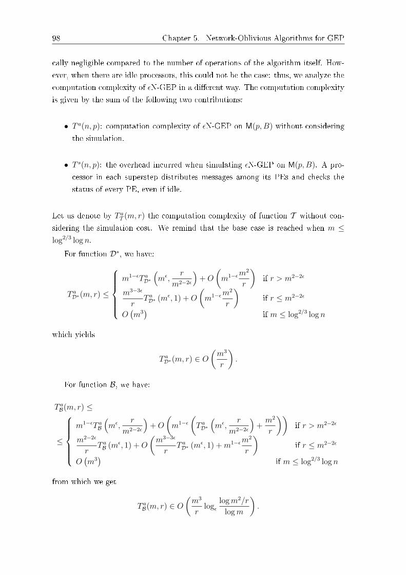
98 Chapter 5. Network-Oblivious Algorithms for GEP
cally negligible compared to the number of operations of the algorithm itself. How-
ever, when there are idle processors, this could not be the case: thus, we analyze the
computation complexity of εN-GEP in a dierent way. The computation complexity
is given by the sum of the following two contributions:
• T a(n, p): computation complexity of εN-GEP on M(p,B) without considering
the simulation.
• T s(n, p): the overhead incurred when simulating εN-GEP on M(p,B). A pro-
cessor in each superstep distributes messages among its PEs and checks the
status of every PE, even if idle.
Let us denote by T aT (m, r) the computation complexity of function T without con-
sidering the simulation cost. We remind that the base case is reached when m ≤log2/3 log n.
For function D∗, we have:
T aD∗(m, r) ≤
m1−εT aD∗
(mε,
r
m2−2ε
)+O
(m1−εm
2
r
)if r > m2−2ε
m3−3ε
rT aD∗ (mε, 1) +O
(m1−εm
2
r
)if r ≤ m2−2ε
O(m3)
if m ≤ log2/3 log n
which yields
T aD∗(m, r) ∈ O(m3
r
).
For function B, we have:
T aB(m, r) ≤
≤
m1−εT aB
(mε,
r
m2−2ε
)+O
(m1−ε
(T aD∗
(mε,
r
m2−2ε
)+m2
r
))if r > m2−2ε
m2−2ε
rT aB (mε, 1) +O
(m3−3ε
rT aD∗ (mε, 1) +m1−εm
2
r
)if r ≤ m2−2ε
O(m3)
if m ≤ log2/3 log n
from which we get
T aB(m, r) ∈ O(m3
rlogε
logm2/r
logm
).

5.2. Network-Oblivious Algorithms 99
Finally, T aA(m, r) is bounded by this recurrence:
T aA(m, r) ≤
≤
m1−εT aA
(mε,
r
m2−2ε
)+O
(m1−ε
(T aB
(mε,
r
m2−2ε
)+ T aD∗
(mε,
r
m2−2ε
)+m2
r
))if r > m2−2ε
m1−εT aA (mε, 1) +O
(m2−2ε
rT aB (mε, 1) +
m3−3ε
rT aD∗ (mε, 1) +m1−εm
2
r
)if r ≤ m2−2ε
O(m3)
if m ≤ log2/3 log n
which provides the following equation:
T aA(m, r) ∈ O(m3
rlog2
ε
logm2/r
logm
).
Since ε is a constant in (0, 1), we obtain:
T a(n, p) = T aA(n, p) ∈ O(n3
plog2 log n
log(n2/p)
).
The cost of message distribution is upper bounded by T a(n, p), since each PE
performs an operation on every sent/received message and a naïve distribution
requires O (1) operations per message; therefore, we ignore it in T s(n, p). Since
each processor performs O (1) operations per PE in each superstep, we have that
T s(n, p) = O ((h(n)/p)Λ(n)), where Λ(n) denotes the number of supersteps of εN-
GEP inM(h(n)). We dene by ΛT (n), with T ∈ A,B,D, the number of superstepsin T . Let `(n) =
√n2/h(n) = log2/3 log n. Since each phase of A, B and D∗ consists
of a constant number of supersteps, it is not dicult to see that:
ΛD∗(m) ≤
m1−εΛD∗(m
ε) +O (m1−ε) if m > `(n)
0 if m ≤ `(n),
which yields
ΛD∗(m) ∈ O(
m
`(n)
).
Similarly, it can be proved that:
ΛB(m) ∈ O(
m
`(n)logε
log `(n)
logm
), ΛA(m) ∈ O
(m
`(n)log2
ε
log `(n)
logm
).

100 Chapter 5. Network-Oblivious Algorithms for GEP
Since ε is a constant in (0, 1) and by setting m = n, it follows that
T s(n, p) ∈ O(
n2
l2(n)pΛA(n)
)∈ O
(n3
l(n)3plog2 log n
log l(n)
)∈ O
(n3
p
).
Note that, if εN-GEP were specied in an M(n2), the cost of simulation would have
been asymptotically bigger that the number of operations due to εN-GEP itself. For
this reason, εN-GEP has been described on M(h(n)), with h(n) = n2/ log4/3 log n.
Equation 5.12 follows since TεN−GEP(n, p,B) ∈ O (T a(n, p) + T s(n, p)).
Corollary 5.9. Let ε be a constant in (0, 1). A commutative GEP computation on an
n×n matrix can be performed by εN-GEP on an M(p,B) with optimal communication
and computation complexities when p ≤ n2−δ, with δ an arbitrary constant in (0, 2),
and B ≤ (n/√p)1+ε.
Proof. The proof descends from Theorem 5.8, and can be proved as Corollary 5.3.
N-GEP exhibits optimal communication and computation complexities for a
wider range of values of p than εN-GEP; however the restriction on the block size
B is less restrictive in εN-GEP. Since the assumption on the block B in N-GEP is
likely to be satised in practical scenarios and εN-GEP requires strong assumptions
on the integrality of the quantities involved, N-GEP is more appealing than εN-GEP.
Nevertheless, εN-GEP is still interesting because it is a parametric algorithm which
becomes N-GEP when ε = 1 − 1/ logm, and becomes PN-GEP (described in the
next section) when ε = 0. Moreover, observe that, by increasing ε by a constant
factor, εN-GEP achieves optimality for bigger communication block sizes, whilst its
communication and computation complexities increase by a constant factor.
εN-GEP requires the matrix on which the GEP computation will be applied
to be distributed among the PEs according with the bit-interleaved layout. This
assumption can be relaxed and, by means of a network-oblivious algorithm similar
to the one in Section 4.2.2 for matrix transposition, a row or column-major layout
can be used. However, the new implementation exhibits optimal communication
complexity on M(p,B) if p ≤ n2−δ, for an arbitrary constant δ in (0, 2), and B ≤minn, (n/√p)1+ε.
It must be remarked that εN-GEP does not satisfy the fullness assumption since,
when p ≤ n2−2ε, the PEs that a processor is simulating send O (n2/p) messages,
however only O(n1+ε√p
)of these are addressed outside the processor. We do not

5.2. Network-Oblivious Algorithms 101
analyze the communication time of εN-GEP in a D-BSP, however note that it requires
O (n1−ε) 0-supersteps, while N-GEP uses only O (1) 0-supersteps.
εN-GEP is not of appealing in practical scenarios for requiring strong assump-
tions on the integrality of the quantities involved. Nevertheless, it is still interesting
because it is a parametric algorithm which becomes N-GEP when ε = 1− 1/ logm,
and becomes PN-GEP when ε = 0. Moreover, by increasing ε by a constant fac-
tor, εN-GEP achieves optimality for bigger communication block sizes, whilst its
communication and computation complexities increase by a constant factor.
5.2.3 PN-GEP
PN-GEP (Pipelined GEP) is a network-oblivious algorithm for performing any GEP
computation, whose specication is given in M(n2). It is a reminiscent of the systolic
algorithm proposed by Lewis and Kung in [LK91] for the algebraic path problems,
which are special cases of GEP computations and include Floyd-Warshall all-pairs
shortest paths and matrix multiplication.
The algorithm descends from function A of εN-GEP by setting5 ε = 0. Speci-
cally, PN-GEP partitions the n × n input matrix into n2 submatrices of size 1 × 1,
thus dening n3 subproblems. Subproblems, which fall immediately into the base
cases, are solved as in εN-GEP's function A. It is immediate to see that PN-GEP
implements correctly all GEP computations for which I-GEP is correct, although
correctness in the general case can be achieved by modifying the algorithm using
similar techniques to those employed in C-GEP [CR07].
The following theorem and corollary show the optimality of PN-GEP on an
M(p,B), for all values of p and a wide range of values of B. Note also that the
restriction to commutative GEP computations is not needed in this case.
Theorem 5.10. A GEP computation on an n× n matrix can be performed by PN-
GEP with communication and computation complexities
HN−GEP (n, p,B) ∈ O(
n2
B√p
+ n
), (5.15)
TN−GEP (n, p,B) ∈ Θ
(n3
p
)(5.16)
on an M(p,B), with 1 < p ≤ n2 and B ≥ 1.
Proof. Each M(p,B) processor holds an n/√p × n/√p submatrix of PEs, but only
PEs on the border send messages outside the processor. Since the algorithm is com-
5εN-GEP is dened when 0 < ε < 1, but function A is well dened when ε = 0.

102 Chapter 5. Network-Oblivious Algorithms for GEP
posed of Θ (n) supersteps, Equations 5.15 and 5.16 follows.
Corollary 5.11. A commutative GEP computation on an n× n matrix can be per-
formed by PN-GEP with optimal communication and computation complexities when
1 < p ≤ n2 and 1 ≤ B ≤ n/√p.
Proof. The proof is straightforward.
Although, PN-GEP yields optimal computation and communication complexities
in the evaluation model for a wide range of the parameters, it is not optimal in a
D-BSP. Indeed, PN-GEP uses only 0-supersteps and does not exploit the hierarchical
structure of the D-BSP interconnection topology.

Chapter 6
Conclusions
Philosophically, the reason research in
math matters is that by pursuing math
ideas that are deep and interesting for
their own sake, you will get real-world
applications in the future.
(Steven Hofmann)
In this nal chapter we summarize the main contributions of the thesis and discuss
some future research directions.
6.1 Summary
In this thesis we contributed novel results on oblivious algorithms, pursuing two main
directions: the investigation of the potentialities and intrinsic limitations of oblivious
versus aware algorithms, and the introduction of the notion of oblivious algorithm
in parallel setting.
In Chapter 3, we studied various aspects concerning the execution of rational
permutations in a cache-RAM hierarchy focusing, in particular, on the oblivious set-
tings. We rst proved a lower bound on the work complexity of any algorithm that
executes rational permutations with optimal cache complexity. By virtue of this
bound we were able to show the work optimality of the cache-aware algorithm deriv-
able from the one in [Cor93a], which also exhibits optimal cache complexity. Then,
we developed a cache-oblivious algorithm for performing any rational permutation,
which exhibits optimal cache and work complexities under the tall-cache assump-
tion. When the rational permutation is a matrix transposition, our cache-oblivious
algorithm represents an iterative version of the recursive cache-oblivious algorithm
103

104 Chapter 6. Conclusions
given in [FLPR99]. Finally, we investigate the separation in asymptotic complex-
ity between cache-aware and cache-oblivious algorithms, showing that for certain
families of rational permutations, including matrix transposition and bit-reversal, a
cache-oblivious algorithm which achieves optimal cache complexity for all values of
the Ideal Cache parameters cannot exist, while this is attainable through a cache-
aware algorithm. This result specializes to the case of rational permutations the
result proved in [BF03] for general permutations, and it is achieved by means of a
simulation technique which formalizes the approach used in [BF03]. To the best of
our knowledge, the only impossibility results of the kind presented in this chapter
and in [BF03], were proved in [BP01]. These results provide interesting insights
on the trade-o between eciency and portability of cache-oblivious algorithms, and
also shed light on the interaction of algorithms with the Translation Lookaside Buer
(TLB) which, if regarded as a cache, does generally not satisfy the tall-cache assump-
tion [Kum03]. Indeed, several algorithms, even if aware, do not use TLB parameters,
and with respect to this component they are oblivious.
In Chapter 4, we proposed a framework for the study of oblivious algorithms in
the parallel setting. This framework explores the design of bulk-synchronous parallel
algorithms that, without resorting to parameters for tuning the performance on the
target platform, can execute eciently on parallel machines with dierent degree of
parallelism and bandwidth characteristics. A network-oblivious algorithm is designed
on the specication model, which consists of a clique of processor/memory pairs,
called processing elements, whose number is function exclusively of the input size.
Then, the communication and computation complexities of the network-oblivious
algorithm are analyzed in the evaluation model, which is similar to the specication
model but provides two parameters, namely processor number and communication
block-size, which capture parallelism and granularity of communication. Finally, the
algorithm is run on the execution model, which is a block-variant of the D-BSP
model. The framework is appealing because, as proved in the thesis, for a wide
class of network-oblivious algorithms, optimality in the evaluation model implies op-
timality in the D-BSP model. We showed that a number of key problems, namely
matrix multiplication and transposition, discrete Fourier transform and sorting, ad-
mit network-oblivious algorithms which are optimal for a wide range of machine
parameters. We also present a further result on the separation between oblivious
and aware approaches, showing the impossibility of designing a network-oblivious
algorithm for matrix transposition which is optimal for all values of the evaluation
model parameters, while this is attainable through an aware parallel approach.
Finally, in Chapter 5 we presented three algorithms, called N-GEP, εN-GEP

6.2. Further research 105
and PN-GEP, for solving a wide class of computations encompassed by the Gaussian
Elimination Paradigm [CR06], which includes all-pairs shortest paths, Gaussian elim-
ination without pivoting and matrix multiplication. They are based on the parallel
and cache-oblivious implementations of the GEP paradigm given in [CR07, CR08],
and perform optimally in the evaluation model for dierent ranges of the parameters.
In particular, εN-GEP and PN-GEP exploit large communication block size and an
high number of processors, respectively, better than N-GEP. However, N-GEP is
more appealing since we proved that it is also optimal in the D-BSP model for some
ranges of the parameters, while this is not the case for PN-GEP and we conjecture
for εN-GEP as well.
6.2 Further research
An interesting avenue for further research is to continue the study of the theoretical
separation between oblivious and aware approaches, for instance, by proving impos-
sibility results similar to those presented in this thesis and in previous works, for
other fundamental problems. Moreover, deeper investigations are required to under-
stand why the tall-cache and small-block assumptions are so crucial in certain cases
to obtain optimal cache and network-oblivious algorithms.
The network-oblivious framework oers several interesting directions for further
work. Naturally, one goal is to design ecient network-oblivious algorithms for other
important problems, beyond the ones proposed in this thesis. Another issue regards
the necessity of the assumptions made in Theorem 4.5 to prove that optimality in
the evaluation model translates into optimality in the D-BSP. In fact, in the thesis
we developed a network-oblivious algorithm, N-GEP, which does not satises these
assumptions, and yet it is optimal in a D-BSP for certain ranges of the parameters.
It is evident that assumptions in the theorem are too conservative. Furthermore,
it would be interesting to study the relations between optimality in the evaluation
model and optimality in other execution models alternative to the D-BSP.
So far the network-oblivious framework and the algorithms developed as case
studies have been investigated only from a theoretical perspective by means of asymp-
totic analysis. Cache-oblivious algorithms are fully compatible with actual platforms
in the sense that the simulation of the specication model in the execution model
is performed by the system through automatic replacement policies of cache lines.
An analogous simulation tool is not available for running network-oblivious algo-
rithms on parallel architectures. Hence, the realization of a library to support the
execution of network-oblivious algorithms is of fundamental importance for assessing

106 Chapter 6. Conclusions
experimentally the actual performance attained by this type of algorithms.
Finally, another interesting research work is to develop new compiling techniques
or to design specic architectural features which provide (a more) eective support
to the execution of oblivious algorithms. One example, as noted in [Fri99], is the
development of techniques to reduce the cost of procedure calls which are useful
in cache and network-oblivious algorithms. Another one is the identication of fast
techniques to support execution of large number of light threads, that would be useful
for the simulation of processing elements of the specication model in processors of
the execution model in the network-oblivious framework.

Appendix A
Properties of Function f (x)
We prove some lemmas that have been used in Chapter 3. Remind that the convex
function f(x) is dened as follows:
f(x) =
x log x if x > 0
0 if x = 0.
Lemma A.1. If bi ≥ 0 for each i, with 0 ≤ i < k, and∑k−1
i=1 bi ≤ b0, then
f
(b0 −
k−1∑i=1
bi
)+
k−1∑i=1
f(bi) ≤ f(b0).
Proof. Without loss of generality we suppose bi > 0 for each i, with 0 ≤ i < k, and∑k−1i=1 f(bi) > f(b0). (The general case is a simple adaptation.) By the denition of
f we get:
f
(b0 −
k−1∑i=1
bi
)+
k−1∑i=1
f(bi) =
(b0 −
k−1∑i=1
bi
)log
(b0 −
k−1∑i=1
bi
)+
(k−1∑i=1
bi log bi
)
≤
(b0 −
k−1∑i=1
bi
)log b0 +
(k−1∑i=1
bi
)log b0 = f(b0).
Lemma A.2. Let a = (a0, . . . , as−1) and ak > 0 for each k, with 0 ≤ k < s. The
function
F (a) = f
(s−1∑k=0
ak
)−
s−1∑k=0
f (ak)
is concave and non decreasing for each ak, with 0 ≤ k < s.
107

108 Appendix A. Properties of Function f(x)
Proof. Let H(a) be the Hessian matrix of F (a) and denote with hi,j(a) the entry
of H in the i-th row and j-th column, that is, the second order partial derivative
of function F (a) with respect to variables aj and ai (in the given order). It is not
dicult to see that:
hi,j(a) =
1∑s−1k=0 ak
if i 6= j
1∑s−1k=0 ak
− 1
aiif i = j
.
Let x = (x0, . . . , xn−1) and x ∈ Rs. We get:
xH(a)xT = − 1∑s−1k=0 ak
s−1∑i=0
s−1∑j=0
(√aiajxi −
√ajaixj
)2
≤ 0
Hence, H(a) is a negative semidenite matrix and F (a) is concave.
Since the rst order partial derivatives of F (a) are non negative when ak > 0 for
each k, with 0 ≤ k < s, F (a) is non decreasing for each ak.
Lemma A.3. Let A be an r × s matrix, with r, s ≥ 1, and denote with ai,j ≥ 0 the
entry of A in the i-th row and j-th column. For 0 ≤ j < s let Mj be a xed value
such that∑r−1
i=0 ai,j ≤Mj. Then an upper bound on the function
F (A) =r−1∑i=0
[f
(s−1∑j=0
ai,j
)−
s−1∑j=0
f (ai,j)
](A.1)
is given by setting ai,j = Mj/r for all i and j, with 0 ≤ i < r and 0 ≤ j < s.
Proof. Suppose ai,j > 0 for each i and j, with 0 ≤ i < r and 0 ≤ j < s. F (A) can
be rewritten as follows:
F (A) = rr−1∑i=0
F ((ai,0, . . . , ai,s−1))
r.
Since F (·) is concave, we can apply the multivariate Jensen's inequality [Neu90]:
F (A) ≤ rF
(r−1∑i=0
(ai,0, . . . , ai,s−1)
r
)
≤ rF
((r−1∑i=0
ai,0r, . . . ,
r−1∑i=0
ai,s−1
r
))

109
Since∑r−1
i=0 ai,j ≤Mj and F (·) is non decreasing for each component, we get:
F (A) ≤r−1∑i=0
F
((M0
r, . . . ,
Ms−1
r
))
≤r−1∑i=0
[f
(s−1∑j=0
Mj
r
)−
s−1∑j=0
f
(Mj
r
)],
from which the lemma follows. The previous equation is an upper bound on F (A)
even if there are some ai,j = 0 since F (·) is continuous and non decreasing in each
component.
Corollary A.4. Let A be an r×s matrix, with r, s ≥ 1, and denote with ai,j the entry
of A in the i-th row and j-th column. Let M0 and M be two xed values such that∑r−1i=0 ai,0 ≤ M0 and
∑s−1j=1
∑r−1i=0 ai,j ≤ M . Then, an upper bound to function F (A),
dened in Equation A.1, is given by setting ai,0 = M0/r and ai,j = M/(r(s− 1)) for
each i and j, with 0 ≤ i < r and 1 ≤ j < s.
Proof. Let Mj denote the partial sum∑r−1
i=0 ai,j for each j with 0 ≤ j < s. By
Lemma A.3, we have that
F (A) ≤r−1∑i=0
[f
(s−1∑j=0
Mj
r
)−
s−1∑j=0
f
(Mj
r
)].
≤r−1∑i=0
[f
(M0
r+
s−1∑j=1
M
r(s− 1)
)− f
(M0
r
)]−
r−1∑i=0
s−1∑j=1
f
(Mj
r
). (A.2)
For the Jensen's inequality, we have:
−r−1∑i=0
s−1∑j=1
f
(Mj
r
)≤ −
r−1∑i=0
s−1∑j=1
f
(M
r(s− 1)
).
Thus,the following upper bound on F (A) follows:
F (A) ≤r−1∑i=0
[f
(M0
r+
s−1∑j=1
M
r(s− 1)
)− f
(M0
r
)−
s−1∑j=1
f
(M
r(s− 1)
)].

110 Appendix A. Properties of Function f(x)

Appendix B
Pseudocode of PI-GEP1 and
PI-GEP2
In this appendix, we reproduce the pseudocode of the two implementations of I-
GEP described in [CR07] and [CR08] for a CREW (concurrent read, exclusive write)
shared-memory model composed of p processors and one level of cache that can be
either shared or distributed. We refer to them as PI-GEP1 and PI-GEP2, respec-
tively. The initial call in both algorithms is A(x, n), where x is the n × n input
matrix of the GEP computation.
A(X,m)INPUT: matrix X ≡ x[I, I] with I = [i0, i1] ⊆ [0, n) with m = i1 − i0 + 1.OUTPUT: execution of all updates 〈i, j, k〉 ∈ T , with T = Σf ∩ (I × I × I).1: if T = ∅ then return;2: if m = 1 then3: X[i0, i0]← f(X[i0, i0], X[i0, i0], X[i0, i0], X[i0, i0]);4: else
5: A(X0,0,m/2);6: In parallel invoke B(X0,1, X0,0,m/2), C(X1,0, X0,0,m/2)7: D(X1,1, X1,0, X0,1, X0,0,m/2);8: A(X1,1,m/2);9: In parallel invoke B(X1,0, X1,1,m/2), C(X0,1, X1,1,m/2);10: D(X0,0, X0,1, X1,0, X1,1,m/2);
Figure B.1: Function A of PI-GEP1[CR07].
111

112 Appendix B. Pseudocode of PI-GEP1 and PI-GEP2
B(X,U,m)INPUT: matrices X ≡ x[I, J ] and U ≡ x[I, I], with I = [i0, i1] ⊆ [0, n), J = [j0, j1] ⊆
[0, n), I ∩ J = ∅ and m = i1 − i0 + 1 = j1 − j0 + 1.OUTPUT: execution of all updates 〈i, j, k〉 ∈ T , with T = Σf ∩ (I × J × I).1: if T = ∅ then return;2: if m = 1 then3: X[i0, i0]← f(X[i0, j0], U [i0, i0], X[i0, j0], U [i0, i0]);4: else
5: parallel: B(X0,0, U0,0,m/2),B(X0,1, U0,0,m/2);6: parallel: D(X1,0, U1,0, X0,0, U0,0,m/2),D(X1,1, U1,0, X0,1, U0,0,m/2);7: parallel: B(X1,0, U1,1,m/2),B(X1,1, U1,1,m/2);8: parallel: D(X0,0, U0,1, X1,0, U1,1,m/2),D(X0,1, U0,1, X1,1, U1,1,m/2);
Figure B.2: Function B of PI-GEP1[CR07].
C(X,V,m)INPUT: matrices X ≡ x[I, J ] and V ≡ x[J, J ], with I = [i0, i1] ⊆ [0, n), J = [j0, j1] ⊆
[0, n), I ∩ J = ∅ and m = i1 − i0 + 1 = j1 − j0 + 1.OUTPUT: execution of all updates 〈i, j, k〉 ∈ T , with T = Σf ∩ (I × J × J).1: if T = ∅ then return;2: if m = 1 then3: X[i0, j0]← f(X[i0, j0], X[i0, j0], V [j0, j0], V [j0, j0]);4: else
5: parallel: C(X0,0, V0,0,m/2), C(X1,0, V0,0,m/2);6: parallel: D(X0,1, X0,0, V0,1, V0,0,m/2),D(X1,1, X1,0, V0,1, V0,0,m/2);7: parallel: C(X0,1, V1,1,m/2), C(X1,1, V1,1,m/2);8: parallel: D(X0,0, X0,1, V1,0, V1,1,m/2),D(X1,0, X1,1, V1,0, V1,1,m/2);
Figure B.3: Function C of PI-GEP1[CR07].
D(X,U, V,W,m)INPUT: matrices X ≡ x[I, J ], U ≡ x[I,K], V ≡ x[K,J ] and W ≡ x[K,K], with I =
[i0, i1] ⊆ [0, n), J = [j0, j1] ⊆ [0, n), K = [k0, k1] ⊆ [0, n), I ∩K = ∅, J ∩K = ∅ andm = i1 − i0 + 1 = j1 − j0 + 1 = k1 − k0 + 1.
OUTPUT: execution of all updates 〈i, j, k〉 ∈ T , with T = Σf ∩ (I × J ×K).1: if T = ∅ then return;2: if m = 1 then3: X[i0, j0]← f(X[i0, j0], U [i0, k0], V [k0, j0],W [k0, k0]);4: else
5: parallel: D(X0,0, U0,0, V0,0,W0,0,m/2),D(X0,1, U0,0, V0,1,W0,0,m/2),D(X1,0, U1,0, V0,0,W0,0,m/2),D(X1,1, U1,0, V0,1,W0,0,m/2);
6: parallel: D(X0,0, U0,1, V1,0,W1,1,m/2),D(X0,1, U0,1, V1,1,W1,1,m/2),D(X1,0, U1,1, V1,0,W1,1,m/2),D(X1,1, U1,1, V1,1,W1,1,m/2).
Figure B.4: Function D of PI-GEP1[CR07].

113
A(X,m)1: As in Lines 1-4 of A in Figure B.1;2: for k ← 0 to r − 1 do
3: A(Xk,k,m/r);4: parallel: B(Xk,j , Xk,k,m/r), C(Xi,k, Xk,k,m/r), for all 0 ≤ i, j < r and
i, j 6= k;5: parallel: D(Xi,j , Xi,k, Xk,j , Xk,k,m/r), for all 0 ≤ i, j < r and i, j 6= k;
B(X,U,m)1: As in Lines 1-4 of B in Figure B.2;2: for k ← 0 to r − 1 do
3: parallel: B(Xk,j , Uk,k,m/r), for all 0 ≤ j < r and j 6= k;4: parallel: D(Xi,j , Ui,k, Xk,j , Uk,k,m/r), for all 0 ≤ i, j < r and i, j 6= k;
C(X,V,m)1: As in Lines 1-4 of C in Figure B.3;2: for k ← 0 to r − 1 do
3: parallel: C(Xi,k, Vk,k,m/r), for all 0 ≤ i < r and i 6= k;4: parallel: D(Xi,j , Xi,k, Vk,j , Vk,k,m/r), for all 0 ≤ i, j < r and i, j 6= k;
D(X,U, V,W,m)1: As in Lines 1-4 of D in Figure B.4;2: for k ← 0 to r − 1 do
3: parallel: D(Xi,j , Ui,k, Vk,j ,Wk,k,m/r), for all 0 ≤ i, j < r;
Figure B.5: Functions A, B, C and D of PI-GEP2 [CR08].

114 Appendix B. Pseudocode of PI-GEP1 and PI-GEP2

Bibliography
[AACS87] Alok Aggarwal, Bowen Alpern, Ashok K. Chandra, and Marc Snir. A
model for hierarchical memory. In Proceedings of the 19th ACM Sympo-
sium on Theory of Computing, pages 305314, 1987.
[ABC+06] Krste Asanovic, Ras Bodik, Bryan Christopher Catanzaro, Joseph James
Gebis, Parry Husbands, Kurt Keutzer, David A. Patterson,
William Lester Plishker, John Shalf, Samuel Webb Williams, and
Katherine A. Yelick. The landscape of parallel computing research: A
view from Berkeley. Technical Report UCB/EECS-2006-183, EECS De-
partment, University of California, Berkeley, December 2006.
[ABF05] Lars Arge, Gerth Stølting Brodal, and Rolf Fagerberg. Cache-oblivious
data structures. In Dinesh P. Mehta and Sartaj Sahni, editors, Handbook
of Data Structures and Applications, chapter 34, page 27. CRC Press,
2005.
[ACFS94] Bowen Alpern, Larry Carter, Ephraim Feig, and Ted Selker. The uniform
memory hierarchy model of computation. Algorithmica, 12(2/3):72109,
1994.
[ACS87] Alok Aggarwal, Ashok K. Chandra, and Marc Snir. Hierarchical memory
with block transfer. In Proceedings of the 28th IEEE Symposium on
Foundations of Computer Science, pages 204216, 1987.
[ACS90] Alok Aggarwal, Ashok K. Chandra, and Marc Snir. Communication
complexity of PRAMs. Theoretical Computer Science, 71:328, 1990.
[Aea02] Narasimha R. Adiga and et al. An overview of the BlueGene/L su-
percomputer. In Proceedings of the ACM/IEEE Conference on Super-
computing, pages 122, Los Alamitos, CA, USA, 2002. IEEE Computer
Society Press.
[Aeo] AEOLUS project website http://aeolus.ceid.upatras.gr.
115

116 Bibliography
[AHU74] Alfred V. Aho, John E. Hopcroft, and Jerey D. Ullman. The Design
and Analysis of Computer Algorithms. Addison-Wesley, 1974.
[Arg04] Lars Arge. External geometric data structures. In Kyung-Yong Chwa
and J. Ian Munro, editors, Proceedings of the 10th Annual International
Conference of Computing and Combinatorics, volume 3106 of Lecture
Notes in Computer Science. Springer, 2004.
[Arv81] Arvind. Data ow languages and architecture. In Proceedings of the 8th
Annual Symposium on Computer Architecture, 1981.
[AV88] Alok Aggarwal and Jerey Scott Vitter. The input/output complexity of
sorting and related problems. Communications of the ACM, 31(9):1116
1127, 1988.
[Bac78] John K. Backus. Can programming be liberated from the Von Neumann
style? A functional style and its algebra of programs. Communication
of the ACM, 21(8):613641, 1978.
[BBP99] Sandeep N. Bhatt, Gianfranco Bilardi, and Geppino Pucci. Area-
universal circuits with constant slowdown. In Proceedings of the 18th
International Conference on Advanced Research in VLSI, pages 8998,
1999.
[BDadH98] Armin Bäumker, Wolfgang Dittrich, and Friedhelm Meyer auf der Heide.
Truly ecient parallel algorithms: 1-optimal multisearch for an exten-
sion of the BSP model. In Selected papers from the 3rd European Sym-
posium on Algorithms, pages 175203, Amsterdam, The Netherlands,
1998. Elsevier Science Publishers B. V.
[BDP99] Armin Bäumker, Wolfgang Dittrich, and Andrea Pietracaprina. The
complexity of parallel multisearch on coarse-grained machines. Algorith-
mica, 24(3-4):209242, 1999.
[Bel66] Laszlo A. Belady. A study of replacement algorithms for a virtual storage
computer. IBM Systems Journal, 5(2):78101, 1966.
[Ber08] Alberto Bertoldo. An adaptive parallel solver for nite-elements appli-
cations. PhD thesis, Department of Information Engineering, University
of Padova, 2008.

Bibliography 117
[BF03] Gerth Stølting Brodal and Rolf Fagerberg. On the limits of cache-
obliviousness. In Proceedings of the 35th ACM Symposium on Theory of
Computing, pages 307315, June 2003.
[BFGK05] Michael A. Bender, Jeremy T. Fineman, Seth Gilbert, and Bradley C.
Kuszmaul. Concurrent cache-oblivious B-trees. In Proceedings of the
17th ACM Symposium on Parallelism in Algorithms and Architectures,
pages 228237, New York, NY, USA, 2005. ACM.
[BFPP01] Gianfranco Bilardi, Carlo Fantozzi, Andrea Pietracaprina, and Geppino
Pucci. On the eectiveness of D-BSP as a bridging model of parallel
computation. In Proceedings of the International Conference on Com-
putational Science-Part II, volume 2074 of Lecture Notes in Computer
Science, pages 579588, London, UK, 2001. Springer-Verlag.
[BP97] Gianfranco Bilardi and Franco Preparata. Processor-time tradeos un-
der bounded-speed message propagation: Part I, upper bounds. Theory
of Computing Systems, 30:523546, 1997.
[BP99] Gianfranco Bilardi and Franco Preparata. Processor-time tradeos un-
der bounded-speed message propagation: Part II, lower bounds. Theory
of Computing Systems, 32:531559, 1999.
[BP01] Gianfranco Bilardi and Enoch Peserico. A characterization of temporal
locality and its portability across memory hierarchies. In Proceedings
of the 28th International Colloquium on Automata, Languages and Pro-
gramming, volume 2076 of Lecture Notes in Computer Science, pages
128139, 2001.
[BPP99] Gianfranco Bilardi, Andrea Pietracaprina, and Geppino Pucci. A quan-
titative measure of portability with application to bandwidth-latency
models for parallel computing. In Proceedings of the 5th International
Euro-Par Conference on Parallel Processing, volume 1685 of Lecture
Notes in Computer Science, pages 543551, September 1999.
[BPP+05] Gianfranco Bilardi, Andrea Pietracaprina, Geppino Pucci, Fabio Schi-
fano, and Raaele Tripiccione. The potential of on-chip multiprocessing
for QCD machines. In Proceedings of the 12th International Confer-
ence on High-Performance Computing, volume 3769 of Lecture Notes in
Computer Science, pages 386397, 2005.

118 Bibliography
[BPP07] Gianfranco Bilardi, Andrea Pietracaprina, and Geppino Pucci. Decom-
posable BSP: A bandwidth-latency model for parallel and hierarchical
computation. In John Reif and Sanguthevar Rajasekaran, editors, Hand-
book of Parallel Computing: Models, Algorithms and Applications, pages
277315. CRC Press, 2007.
[BPPS07] Gianfranco Bilardi, Andrea Pietracaprina, Geppino Pucci, and
Francesco Silvestri. Network-oblivious algorithms. In Proceedings of the
21st IEEE International Parallel and Distributed Processing Symposium,
March 2007.
[CFSV95] Thomas Cheatham, Amr F. Fahmy, Dan C. Stefanescu, and Leslie G.
Valiant. Bulk synchronous parallel computing - a paradigm for trans-
portable software. In Proceedings of the 28th Hawaii International Con-
ference on System Sciences, page 268, Washington, DC, USA, 1995.
IEEE Computer Society.
[CG98] Larry Carter and Kang Su Gatlin. Towards an optimal bit-reversal
permutation program. In Proceedings of the 39th IEEE Symposium on
Foundations of Computer Science, pages 544555, 1998.
[Cho07] Rezaul A. Chowdhury. Cache-ecient Algorithms and Data Structures:
Theory and Experimental Evaluation. PhD thesis, Department of Com-
puter Sciences, The University of Texas at Austin, August 2007.
[CKP+96] David E. Culler, Richard M. Karp, David A. Patterson, Abhijit Sa-
hay, Eunice E. Santos, Klaus E. Schauser, Ramesh Subramonian, and
Thorsten von Eicken. LogP: A practical model of parallel computation.
Communications of the ACM, 39(11):7885, November 1996.
[CLPT99] Siddhartha Chatterjee, Alvin R. Lebeck, Praveen K. Patnala, and
Mithuna Thottethodi. Recursive array layouts and fast parallel matrix
multiplication. In Proceedings of the 11th ACM Symposium on Parallel
Algorithms and Architectures, pages 222231, 1999.
[CLPT02] Siddhartha Chatterjee, Alvin R. Lebeck, Praveen K. Patnala, and
Mithuna Thottethodi. Recursive array layouts and fast matrix mul-
tiplication. IEEE Transactions on Parallel and Distributed Systems,
13(11):11051123, November 2002.

Bibliography 119
[CLRS01] Thomas H. Cormen, Charles E. Leiserson, Ronald L. Rivest, and Cliord
Stein. Introduction to Algorithms. The MIT Press, Cambridge, MA,
USA, second edition, September 2001.
[Cor93a] Thomas H. Cormen. Fast permuting on disk arrays. Journal of Parallel
and Distributed Computing, 17(1-2), 1993.
[Cor93b] Thomas H. Cormen. Virtual Memory for Data-Parallel Computing. PhD
thesis, Massachussetts Institute of Technology, 1993.
[CR06] Rezaul A. Chowdhury and Vijaya Ramachandran. Cache-oblivious dy-
namic programming. In Proceedings of the 17th ACM-SIAM Symposium
on Discrete Algorithm, pages 591600, 2006.
[CR07] Rezaul A. Chowdhury and Vijaya Ramachandran. The cache-oblivious
Gaussian elimination paradigm: theoretical framework, parallelization
and experimental evaluation. In Proceedings of the 19th annual Sympo-
sium on Parallelism in Algorithms and Architectures, pages 7180, New
York, NY, USA, 2007. ACM.
[CR08] Rezaul A. Chowdhury and Vijaya Ramachandran. Cache-ecient dy-
namic programming algorithms for multicores. In Proceedings of the
20th Symposium on Parallelism in Algorithms and Architectures, pages
207216, New York, NY, USA, 2008. ACM.
[CSG98] David Culler, J. P. Singh, and Anoop Gupta. Parallel Computer Archi-
tecture: A Hardware/Software Approach. Morgan Kaufmann, August
1998.
[Dem56] Howard B. Demuth. Electronic Data Sorting. PhD thesis, Stanford
University, October 1956.
[Dem85] Howard B. Demuth. Electronic data sorting. IEEE Transactions on
Computers, 34(4):296310, 1985.
[Dem02] Erik Demaine. Cache-oblivious algorithms and data structures. Lecture
Notes from the EEF Summer School on Massive Data Sets, 2002.
[DHMD99] Frank Dehne, David Hutchinson, Anil Maheshwari, and Wolfgang Dit-
trich. Reducing I/O complexity by simulating coarse grained parallel
algorithms. In Proceedings of the 13th International Symposium on Par-
allel Processing and the 10th Symposium on Parallel and Distributed

120 Bibliography
Processing, pages 1420, Washington, DC, USA, 1999. IEEE Computer
Society.
[DlTK95] Pilar De la Torre and Clyde P. Kruskal. A structural theory of re-
cursively decomposable parallel processor-networks. In Proceedings of
the IEEE Symposium on Parallel and Distributeed Processing, page 570,
Washington, DC, USA, 1995. IEEE Computer Society.
[DlTK96] Pilar De la Torre and Clyde P. Kruskal. Submachine locality in the bulk
synchronous setting. In Proceedings of the 2nd International Euro-Par
Conference on Parallel Processing-Volume II, volume 1124 of Lecture
Notes in Computer Science, pages 352358, August 1996.
[Fan03] Carlo Fantozzi. A Computational Model for Parallel and Hierarchical
Machines. PhD thesis, Department of Information Engineering, Univer-
sity of Padova, 2003.
[FIP99] FIPS PUB 46-3. Data Encryption Standard (DES). National Institute
for Standards and Technology, Gaithersburg, MD, USA, October 1999.
[FJ98] Matteo Frigo and Steven G. Johnson. FFTW: an adaptive software
architecture for the FFT. Proceedings of the IEEE International Con-
ference on Acoustics, Speech and Signal Processing, 3:13811384 vol.3,
May 1998.
[FK03] Ian Foster and Carl Kesselman. The Grid 2: Blueprint for a New Com-
puting Infrastructure. Morgan Kaufmann Publishers Inc., San Francisco,
CA, USA, 2003.
[Flo72] Richard W. Floyd. Permuting information in idealized two-level stor-
age. In R. Miller and J. W. Thatche, editors, Complexity of Computer
Computations, pages 105109. Plenum, 1972.
[FLPR99] Matteo Frigo, Charles E. Leiserson, Harald Prokop, and Sridhar Ra-
machandran. Cache-oblivious algorithms. In Proceedings of the 40th
IEEE Symposium on Foundations of Computer Science, pages 285298,
1999.
[FPP03] Carlo Fantozzi, Andrea Pietracaprina, and Geppino Pucci. A general
Pram simulation scheme for clustered machines. International Journal
on Foundations of Computer Science, 14(6):11471164, 2003.

Bibliography 121
[FPP06] Carlo Fantozzi, Andrea Pietracaprina, and Geppino Pucci. Translating
submachine locality into locality of reference. Journal of Parallel and
Distributed Computing, 66(5):633646, 2006.
[Fri99] Matteo Frigo. Portable High-Performance Programs. PhD thesis, Mas-
sachusetts Institute of Technology, June 1999.
[Fri08] Matteo Frigo. Personal communication, 2008.
[FS06] Matteo Frigo and Volker Strumpen. The cache complexity of multi-
threaded cache oblivious algorithms. In Proceedings of the 18th ACM
Symposium on Parallelism in Algorithms and Architectures, pages 271
280, New York, NY, USA, 2006. ACM.
[FW78] Steven Fortune and James Wyllie. Parallelism in random access ma-
chines. In Proceedings of the 10th ACM Symposium on Theory of Com-
puting, pages 114118, New York, NY, USA, 1978. ACM.
[GMR99] Phillip B. Gibbons, Y. Matias, and Vijaya Ramachandran. Can a shared-
memory model serve as a bridging-model for parallel computation? The-
ory of Computing Systems, 32(3):327359, 1999.
[Gol78] Leslie M. Goldschlager. A unied approach to models of synchronous
parallel machines. In Proceedings of the 10th annual ACM symposium
on Theory of computing, pages 8994, New York, NY, USA, 1978. ACM.
[Goo99] Michael T. Goodrich. Communication-ecient parallel sorting. SIAM
Journal on Computing, 29(2):416432, 1999.
[GVL96] Gene H. Golub and Charles F. Van Loan. Matrix Computations. The
Johns Hopkins University Press, October 1996.
[GVW96] Garth A. Gibson, Jerey Scott Vitter, and John Wilkes. Strategic di-
rections in storage I/O issues in large-scale computing. ACM Computer
Survey, 28(4):779793, 1996.
[HK81] Jia-Wei Hong and H. T. Kung. I/O complexity: The red-blue pebble
game. In Proceedings of the 13th ACM Symposium on Theory of Com-
puting, pages 326333, New York, NY, USA, 1981. ACM.
[HP06] John L. Hennessy and David A. Patterson. Computer Architecture,
Fourth Edition: A Quantitative Approach. Morgan Kaufmann Publish-
ers Inc., San Francisco, CA, USA, 2006.

122 Bibliography
[ITT04] Dror Irony, Sivan Toledo, and Alexander Tiskin. Communication lower
bounds for distributed-memory matrix multiplication. Journal of Par-
allel and Distributed Computing, 64(9):10171026, 2004.
[JáJ92] Joseph JáJá. An Introduction to Parallel Algorithms. Addison Wesley
Longman Publishing Co., Inc., Redwood City, CA, USA, 1992.
[KA02] Ken Kennedy and John R. Allen. Optimizing Compilers for Modern
Architectures: A Dependence-based Approach. Morgan Kaufmann Pub-
lishers Inc., San Francisco, CA, USA, 2002.
[Ker70] Leslie Robert Kerr. The eect of algebraic structure on the computa-
tional complexity of matrix multiplication. PhD thesis, Cornell Univer-
sity, 1970.
[Knu98] Donald E. Knuth. Art of Computer Programming, Volume 3: Sorting
and Searching. Addison-Wesley Professional, second edition, April 1998.
[KR90] Richard M. Karp and Vijaya Ramachandran. Parallel algorithms for
shared-memory machines. In Handbook of Theoretical Computer Science,
Volume A: Algorithms and Complexity, pages 869942. MIT Press, 1990.
[Kum03] Piyush Kumar. Cache oblivious algorithms. In Meyer et al. [MSS03],
pages 193212.
[Lei85] Charles E. Leiserson. Fat-trees: universal networks for hardware-ecient
supercomputing. IEEE Transactions on Computers, 34(10):892901, Oc-
tober 1985.
[Lei92] Frank Thomson Leighton. Introduction to Parallel Algorithms and Ar-
chitectures: Arrays • Trees • Hypercubes. Kaufmann, 1992.
[LK91] Paul S. Lewis and Sun-Yuan Kung. An optimal systolic array for the
algebraic path problem. IEEE Transactions on Computers, 40(1):100
105, 1991.
[MHS05] Marjan Merenik, Jan Heering, and Anthony M. Sloane. When and
how to develop domain-speciï¬c languages. ACM Computer Surveys,
37(4):316344, 2005.
[MS00] Kurt Mehlhorn and Peter Sanders. Scanning multiple sequences via
cache memory. Algorithmica, 35:2003, 2000.

Bibliography 123
[MSS03] Ulrich Meyer, Peter Sanders, and Jop F. Sibeyn, editors. Algorithms for
Memory Hierarchies, Advanced Lectures (Dagstuhl Research Seminar,
March 10-14, 2002), volume 2625 of Lecture Notes in Computer Science.
Springer, 2003.
[Neu90] Edward Neuman. Inequalities involving multivariate convex functions
ii. Proceedings of the American Mathematical Society, 109(4):965974,
1990.
[ONH+96] Kunle Olukotun, Basem A. Nayfeh, Lance Hammond, Ken Wilson, and
Kunyung Chang. The case for a single-chip multiprocessor. In Pro-
ceedings of the 7th International Conference on Architectural Support
for Programming Languages and Operating Systems, pages 211. ACM
Press, 1996.
[Pie95] Andrea Pietracaprina. Lower bound for BSPC matrix multiplication.
Manuscript, 1995.
[PPS06] Andrea Pietracaprina, Geppino Pucci, and Francesco Silvestri. Cache-
oblivious simulation of parallel programs. In Proceedings of the 8th Work-
shop on Advances in Parallel and Distributed Computational Models,
April 2006.
[Rah02] Naila Rahman. Algorithms for hardware caches and TLB. In Meyer
et al. [MSS03], pages 171192.
[SCD02] Sandeep Sen, Siddhartha Chatterjee, and Neeraj Dumir. Towards a
theory of cache-ecient algorithms. Journal of the ACM, 49(6):828
858, 2002.
[Sil05] Francesco Silvestri. Simulazione di algoritmi paralleli per il modello
D-BSP su una gerarchia di cache ideali. Master's thesis, Department
of Information Engineering, University of Padova, Italy, October 2005.
Laurea Thesis (in italian).
[Sil06] Francesco Silvestri. On the limits of cache-oblivious matrix transpo-
sition. In Ugo Montanari, Donald Sannella, and Roberto Bruni, edi-
tors, Proceedings of the 2nd Symposium of Trustworthy Global Comput-
ing, volume 4661 of Lecture Notes in Computer Science, pages 233243.
Springer, 2006.

124 Bibliography
[Sil08] Francesco Silvestri. On the limits of cache-oblivious rational permuta-
tions. Theoretical Computer Science, 402(2-3):221233, 2008.
[SK97] Jop F. Sibeyn and Michael Kaufmann. BSP-like external-memory com-
putation. In Proceedings of the 3rd Italian Conference on Algorithms
and Complexity, pages 229240, London, UK, 1997. Springer-Verlag.
[SN96] Elizabeth A.M. Shriver and Mark Nodine. An introduction to parallel
I/O models and algorithms. In Input/output in parallel and distributed
computer systems, pages 3168. Kluwer Academic Publishers, 1996.
[SV87] John E. Savage and Jerey Scott Vitter. Parallelism in space-time trade-
os. In Advances in Computing Research, volume 4, pages 117146.
North-Holland, 1987.
[Tok] Tokutek website: www.tokutek.com.
[Val90] Leslie G. Valiant. A bridging model for parallel computation. Commu-
nications of the ACM, 33(8):103111, August 1990.
[Vit01] Jerey Scott Vitter. External memory algorithms and data structures:
dealing with massive data. ACM Computing Surveys, 33(2):209271,
2001.
[VS94] Jerey Scott Vitter and Elizabeth A.M. Shriver. Algorithms for parallel
memory I: Two-level memories. Algorithmica, 12(2/3):110147, 1994.
[Wol96] Michael Wolfe. Parallelizing compilers. ACM Computer Surveys,
28(1):261262, 1996.
[WPD01] R. Clinton Whaley, Antoine Petitet, and Jack Dongarra. Automated
empirical optimizations of software and the ATLAS project. Parallel
Computing, 27(1-2):335, 2001.
[YRP+07] Kamen Yotov, Thomas Roeder, Keshav Pingali, John A. Gunnels, and
Fred G. Gustavson. An experimental comparison of cache-oblivious and
cache-conscious programs. In Proceedings of the 19th ACM Symposium
on Parallel Algorithms and Architectures, 2007.