Embed Size (px)
Citation preview
Abstract This article examines current account deficit adjustments in selected transitioncountries in the 1990s and at the beginning of the 21st century. For this purpose we primarily investigate the main characteristics of sharp current account reversals in Albania, Armenia, Belarus, Bosnia and Herzegovina, Kyrgyz R., Lithuania, Moldova, Poland, Slovenia and Ukraine. Results suggest that restrictively definedreversals seem to be closely related to factors such as domestic savings, real export growth, international reserves and external indebtedness as well as to budget and trade balances. While the role of exchange rate depreciation seems ambiguous, we found that sharp current account reversals are systematically associated with a gradual GDP growth slowdown in the pre-reversal period and with robust GDP growth impetus afterwards.
JEL Classification: C33, F32, F34Keywords: Current account balance, reversals, macroeconomic, variables, eastern Europe, former Soviet Union
South-Eastern Europe Journal of Economics 1 (2006) 9-45
*Corresponding author: Department of Economics and Public Sector Management, Gosarjeva ul. 5, 1000 Ljubljana, Slovenia, e-mail: [email protected]
We are grateful to annonymous referres, whose comments helped us in improving the content and expostition of the paper. Earlier version of the paper was presented at ‘4th International Symposium Economy & Business 2005: Economic development and growth’ in Bourgas, Bulgaria. Comments from conference participants led to the current version of the paper. The paper is also part of Aleksander Aristovnik’s Ph.D. research titled ‘Current Account Sustainability in Selected Transition Countries’. Any remaining errors and ambiguities are our responsibility.
SOME CHARACTERISTICS OF SHARP CURRENT ACCOUNTDEFICIT REVERSALS IN TRANSITION COUNTRIES
ALEKSANDER ARISTOVNIKa*, ANDREJ KUMARb
University of LjubljanaaFaculty of Administration
bFaculty of Economics
10 A. ARISTOVNIK, A. KUMAR, South-Eastern Europe Journal of Economics 1 (2006) 9-45
1. For instance from an intertemporal perspective, Bussière et al. (2004) found that current accounts in most CEE countries (i.e. new EU member countries) are broadly in line with their structural cur-
1. Introduction
After the centrally planned economy ceased to exist, the process of post-socialist transformation has advanced significantly. 27 countries in central and eastern Europe(CEE), southern and eastern Europe (SEE) and the Commonwealth of Independent States (CIS) have since been involved in vast systematic changes. Undoubtedly, these changes have been leading to full-fledged market economies, although the preciseoutcome of transformation is not going to be the same for all countries involved. In fact, some leaders, i.e. the CEE region, joined the EU in 2004 while others, especially countries of the CIS region, are lagging behind in systematic changes and maintain-ing a hybrid system with remnants of central planning existing alongside elements of market regulation and a growing private sector. However, these changes have in-fluenced their external balances significantly, raising doubts about their sustainabilityand concerns over the potential impact that a rapid and disorderly correction of these imbalances might have. Roubini and Wachtel (1999) argued that the current account deficits seen in transition economies reflect two important aspects. On the one hand,these deficits reflect the success of structural changes that have enabled capital andinvestment inflows and have opened up prospects of fast economic growth. On theother hand, from another perspective current account deficits frequently reflect mis-managed transition processes featuring unsustainable imbalances that are potentially a source of a value or a currency and/or balance of payments crisis (e.g. Czech Rep. (1997), Russia (1998)). In fact, the general view is that postponing current account adjustments increases the costs of adjustment in the economy. However, given that fi-nancial markets in transition countries are gradually beginning to operate efficiently,the deterioration of current account balances might offer good investment opportuni-ties in the region when compared to the rest of the world. Indeed, a growing deficitmight be a sign of the gradual growth of the economic strength of the transition economies and is thus not necessarily a bad thing. In line with this, strong demands have emerged for assessing the sustainability of the current account positions as well as those factors determining the current account deficit reversals of the so far mainly(empirically) neglected transition countries. The current account position’s significance stems from the fact that the current ac-count balance, reflecting the saving-investment ratio, is closely related to the status ofthe budget balance and private savings - which are key factors of economic growth. Practically all transition countries have been involved in their own catching-up proc-esses, which include financing a huge amount of productive investment without en-dangering their external sustainability as far as their current account positions and external debt are concerned.1 In fact, these countries suffer from relatively low and
A. ARISTOVNIK, A. KUMAR, South-Eastern Europe Journal of Economics 1 (2006) 9-45 11
even stagnant saving rates. Hence, to close the gap they need to turn to foreign sav-ing, which has generally induced the high and even growing current account deficitsof the last decade. In this respect, the problem of external imbalances is particularly important for CEE countries which have already expressed their desire to adopt the euro as soon as possible. Consequently, for the new (and other prospective) members of the EU a trade-off has emerged between the catching up process and meeting the qualitative current account Maastricht criteria.2
While there are well-known characteristics of current account reversals in devel-oped countries where, in particular, currency depreciation and a decrease in GDP growth are involved (see e.g. Freund (2000), Debelle and Galati (2005), Clarida et al. (2005), Adalet and Eichengreen (2005) and Croke et al. (2005)) there are few surveys for current account adjustments in transition countries (Roubini and Wachtel (1999), Zanghieri, P. (2004), Melecky (2005)), mainly due to the short time span as well as data unreliability and deficiencies. Therefore, the present paper seeks to fill this gapin at least three analytical directions. First, we examine those factors that might have triggered the reversals and provide some insights into the current account adjustment process. We investigate the role of domestic internal factors such as output growth and domestic savings and external sector factors such as the real effective exchange rate and external indebtedness. We focus on two different reversal episodes, i.e. Reversal I (68 episodes) and Reversal II (10 episodes), where the first one is significantly lessrestrictive. Second, we also try to reveal some characteristics of persistent current ac-count deficits in the region. We identify and examine 10 episodes of current accountdeficit persistency in twelve transition countries. Moreover, we undertake a study ofthe indicators and consequences of current account deficit reversals and persistencyin transition countries over the 1992-2003 period using an analysis similar to Milesi-Ferretti (2000, hereafter ‘MFR’), Freund (2000), Debelle and Galati (2005). Finally, we also examine the direct impact of the reversals on economic growth in the region. The experiences of many emerging market countries in recent years, such as Mexico (in 1994), the Asian countries (1997), and Argentina (2001), set out an association between current account adjustment and GDP growth slowdown. This outcome is also empirically tested and confirmed by recent research into current account adjust-ments in these countries (see MFR (2000) and Edwards (2004)). However, in order to
rent account positions. Nevertheless, one needs to underline that this does not necessarily rule out the possibility of a sharp current account adjustment due to other reasons not included in the model (e.g. liquidity and solvency issues).2. Article 121 (Treaty of the European Union, 1992) states that among other (qualitative) criteria «the situation and the evolution of the balance of current payments» of the applicant countries have to be examined before they enter the Euro Area. Recently, an important step towards the Euro Area was taken by Estonia, Lithuania and Slovenia which joined the ERM II with effect from 28 June 2004 and Latvia from 2 May 2005.
12 A. ARISTOVNIK, A. KUMAR, South-Eastern Europe Journal of Economics 1 (2006) 9-45
examine the external adjustment impact on growth in the transition countries, we - in a way - upgrade the work of Melecky (2005) by extending the time span and number of transition countries included in the sample. The paper is organized as follows. The next section of the paper contains a dis-cussion of some theoretical and empirical issues of the current account reversals. Section 3 summarizes trends and developments in current account balances in transi-tion countries. This section also defines episodes of reversals and the persistency ofcurrent account balances in the region in order to examine the current account ad-justment process in the sample countries. The next section empirically estimates the static effect of a current account reversal on economic growth. Thus, the empirical framework and results from the pooled cross-sectional and time-series data estima-tions with a variety of robustness tests are presented in Section 4. The final sectionprovides concluding remarks.
2. Theoretical Background And Recent Empirical Literature
In his comprehensive review Edwards (2001) describes the evolving views of econo-mists regarding the nature and consequences of current account deficits. The attitudehas changed from ‘the current account matters’ to ‘the current account deficit doesnot matter as long as the public sector is in balance’, then to ‘the current account deficit may matter’. In fact, in the 1970s this elastic approach to the current accountwas placed on the backburner and attention was switched to the intertemporal proper-ties of current account deficits. In terms of national accounting, the current accountis simply the difference between national saving and investment. Since both saving and investment are inherently intertemporal phenomena, e.g. saving with respect to the lifetime of individuals and investment with respect to the expected future return on investment, the same must also hold for the current account. In this respect, Obstfeld and Rogoff (1996) provided an extensive review of mod-ern models of the current account that assume intertemporal optimisation on behalf of consumers and firms. In this type of model (assuming a constant interest rate), con-sumption smoothing across periods is one of the fundamental drivers of the current account. According to the intertemporal approach, if output falls below its permanent value there will be a higher current account deficit. Similarly, if investment increasesabove its permanent value the current account deficit will grow. The reason for this isthat new investment projects will be partially financed by an increase in foreign bor-rowing, thus generating a bigger current account deficit. Likewise, increased govern-ment consumption will result in a higher current account deficit. If the constant worldinterest rate assumption is relaxed, a country’s net foreign asset position and the level of the world interest rate would fundamentally affect the current account deficit. Ac-cordingly, if a country is a net foreign debtor, and the world interest rate exceeds its permanent level, the current account deficit would be higher (Miller, 2002).
A. ARISTOVNIK, A. KUMAR, South-Eastern Europe Journal of Economics 1 (2006) 9-45 13
During the last three decades most financial crises have highlighted the part playedby large current account deficits in the run-up to crisis episodes. Consequently, theconcept of a sustainable current account deficit has become an important theoretical,political and economic issue.3 In this respect, Corsetti et al. (1998) concluded that, on the whole, those countries hit hardest by currency crises were those which had persistent current account deficits throughout the 1990s.4 This result is confirmed byRadelet and Sachs (2000), Kamin et al. (2001), Fischer (2003) and Edwards (2004); Edwards shows that the probability of experiencing abrupt current account reversals is closely linked to the size of current account deficits. Accordingly, although this isnot a universal truth, the conventional wisdom is that current account deficits above5 percent of GDP generally represent a problem, especially if funded through short-term borrowing. However, because of the lasting improvement in capital market ac-cess and as predicted by the intertemporal models, the persistent enhancement of the terms of trade and productivity growth seen in transition countries can financemoderate current account deficits on an ongoing basis. Nevertheless, Edwards (2001)affirmed the relevance of current account imbalances, as there is strong evidence thatlarge current account deficits should be a cause for concern in economic policy. Generally, there is a common view that current account adjustment tends to pro-ceed more smoothly in developed countries as it emerges through marked changes in quantities. The main reasons for the smoother adjustment process in developed countries involve the developed and functioning institutional framework, deep and liquid capital markets, more diversified real economy and the ability to issue liabili-ties in domestic currency. A wide range of literature is devoted to adjustment proc-esses in developed countries. For example, Freund (2000) analyses the adjustment process in 25 developed (industrial) countries. By examining the episodes of current account reversals (between 1980 and 1997), she noted that typical reversals occurred when the current account to GDP ratio reached 5 percent. Further, the reversals were typically characterized by a substantial output growth decline and a 10-20 percent real depreciation of the currency, as well as by an increase in real export growth,
3. According to Milesi-Ferretti and Razin (1996) three different yet interrelated concepts can be distinguished: an economy’s solvency, current account sustainability and current account deficitexcessiveness. First, an economy is treated as solvent if the present discounted value of the future trade surplus is equal to the current external indebtedness. Second, a narrower definition of sol-vency brings us to a more widespread idea i.e. the definition of sustainability. A current accountis sustainable if the continuation of the current government policy stance and/or of present private sector behavior will not entail a need for a ‘drastic’ policy shift or a balance of payments (currency) crisis.4. Finally, an unsustainable deficit should be distinguished from an excessive one, i.e. a deficitwhich is too large to be explained in the terms of any given model of consumption, investment and production.
14 A. ARISTOVNIK, A. KUMAR, South-Eastern Europe Journal of Economics 1 (2006) 9-45
a decline in domestic investment, and some levels off in the budget deficit and thenet international investment position. As she concluded, current account adjustment processes tend to be driven by cyclical factors. Later studies, mostly building on Freund’s (2000) work, yield similar results (sizable economic growth slowdown and large exchange rate depreciations) which have been additionally set out by Edwards (2004), Freund and Warnock (2005), and Debelle and Galati (2005). On the other hand, Croke et al. (2005) could not find that the adjustment process was associatedwith a significant and sustained depreciation of the real exchange rate in developedcountries. Even more, the most substantial depreciation occurred among those epi-sodes where GDP growth picked up during the adjustment. Accordingly, they con-clude that these findings weaken the historical basis for predicting disruptive currentaccount adjustments. On the other hand, significant attention has also focused on examinations of largecurrent account adjustments in low and middle income countries (see e.g. Calvo and Reinhart (1999), MFR (1998, 2000), Edwards (2001, 2004), Calvo (2003)). Gener-ally, they show that variables such as current account balance, openness, the level of reserves, terms of trade shocks, US growth and real interest rate help predict current account reversals in these countries. In particularly extensive research, MFR (1998) examined empirical regularities during current account reversals and currency crises using data from 105 low and middle income countries. In addition to the above find-ings, he concluded that reversals are more likely to occur in countries that have run persistent deficits, in countries with high official transfers and whose debt is largelyon concessional terms. Moreover, reversals are not systematically associated with a decline in output growth and are not strongly associated with a currency crisis (less than one-third of reversals were preceded by a currency crisis). According to up-to-date theoretical and empirical literature we can expect that current account adjustments in transition countries are probably less benign than in developed countries.5 Indeed, external adjustments in transition countries have often involved the abandonment of fixed exchange rate regimes (e.g. Czech R. (1997),Slovakia (1998) and Poland (2000)) and, in those circumstances, it is possible to anticipate the extent of the currency depreciation6 and GDP growth slowdown.7 Fur-
5. Nevertheless, this does not imply that a large deficit always leads to a crisis, nor that a crisis canonly occur if a large current account deficit is present (Summers, 2000).6. Melecky (2005) found that after a current account reversal in central and eastern Europe (in-cluding Malta, Cyprus and some less developed old EU member states) the GDP growth rate had declined by 1.10 percentage points in the current year. In addition, the reversals are likely to be eliminated after 3.3 years when the actual growth rate is restored and the cumulative loss associated with a sudden stop in capital flows is about 2.3 percentage points in the region.7. For example, Edwards (2004) confirms that countries with more flexible exchange rate regimesare better able to accommodate than countries with relatively more fixed exchange rate regimes.
A. ARISTOVNIK, A. KUMAR, South-Eastern Europe Journal of Economics 1 (2006) 9-45 15
thermore, another possible reason for expecting a less benign scenario is that in the transition countries great uncertainty exists about monetary policy and fiscal sol-vency, which leads to greater financial volatility during adjustment episodes than indeveloped countries. Moreover, we can assume that current account reversals in tran-sition countries might be generally reversed because of their internal macroeconomic imbalances. Indeed, as an economy grows domestic demand growth exceeds domes-tic output, which results in a widening trade and current account balance. Growing domestic demand induces the rapid growth of credit and an additional rise in infla-tion. Restrictive monetary policy slows GDP growth down and depresses inflation.The combination of a slowdown in the economy and the resulting easing in monetary policy usually reduces the attractiveness of the domestic economy, resulting in a de-preciation of the exchange rate. In addition, the fiscal position deteriorates as a resultof both fiscal stabilizers as well as imprudent government measures. However, to testthe less benign scenario presented, and to provide some further insights into the cur-rent account adjustment processes in transition countries, different approaches will be applied in the rest of this paper.
3. Current Account Imbalances And Reversals In Transition Countries
3.1 Current account imbalances in transition countries
The overview of the current account balance in transition countries shows that, with the exception of Russia – a major commodity exporter - the opening up to external trade has been accompanied by significant current account deficits (see Table 1). In CEE current account balances were not problematic, with even a moderate posi-tive balance as a share of GDP up until 1994 (averaging around 1 percent of GDP), reflecting contractions in domestic demand, real exchange rate undervaluations andexternal financing constraints. Afterwards, significant current account deficit dete-rioration was observed in the region, peaking at almost 7 percent of GDP in 1998 on average (e.g. Lithuania (11.7), Latvia (10.7) and Slovakia (9.6)), mostly as a result of growing imports of both consumption and investment goods. Moreover, the gradual growth of the current account deficit in the CEE region reflects a combination oflong-term growth and structural factors, external shocks and domestic policies. More precisely, the deterioration of current accounts in the region was the result of the growth of merchandise trade deficits, downward trends in the service balance, risingindebtedness and profit repatriation as well as the consequence of the continuous realappreciation of domestic currency in most cases examined.
16 A. ARISTOVNIK, A. KUMAR, South-Eastern Europe Journal of Economics 1 (2006) 9-45
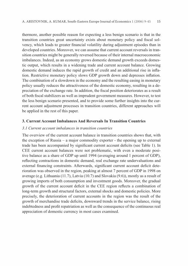
Figure 1. Average current account balance (CA), budget balance (GB) and private balance (PB) in transition countries (in percentage of GDP; unweighted averages).
Similar but even more intensive current account deficit dynamics were seen in theCIS region by achieving the top average current account deficit at a significantlyhigher level (13.7 percent of GDP) than the CEE region in 1998. The major contribu-tors to such a huge deterioration in the current account balance were some countries in the region with current account deficits above 20 percent of GDP (e.g. Turkmeni-stan (37.4), Azerbaijan (30.7) etc.). Several factors contributed to this development. First, many countries in the region experienced large losses in their terms of trade as prices for energy imports from the former Council for Mutual Economic Assistance (CMEA) trading partners moved to market-determined levels. Second, these coun-tries ran high negative fiscal imbalances as authorities tried to absorb the revenue andexpenditure pressure associated with sharp falls in national income and fiscal restruc-turing (see Table 1). Third, as a result of slow progress in building a competitive and diversified export sector trade liberalization mainly stimulated imports of consumergoods and services. As a response to the Russian crisis the average current account deficits narrowed in the group. However, in many cases the deficits remained high– around or even above 10 percent of GDP (Azerbaijan (15.9), Armenia (8.1) etc.) on average in the recent 2001-2003 period. On the other hand, the SEE region achieved
A. ARISTOVNIK, A. KUMAR, South-Eastern Europe Journal of Economics 1 (2006) 9-45 17
the highest average current account deficit with around 20 percent of GDP in 1992due to the enormous deficit seen in Albania (68.5 percent). Later these huge externalimbalances improved significantly. However, at the beginning of the second half ofthe 1990s and in the first years of the 21st century they again deteriorated. Eventually,the average current account deficit was 8.2 percent of GDP in the 2001-2003 periodin comparison to the previous three years when it averaged out at 5.9 percent of GDP (see Figure 1).
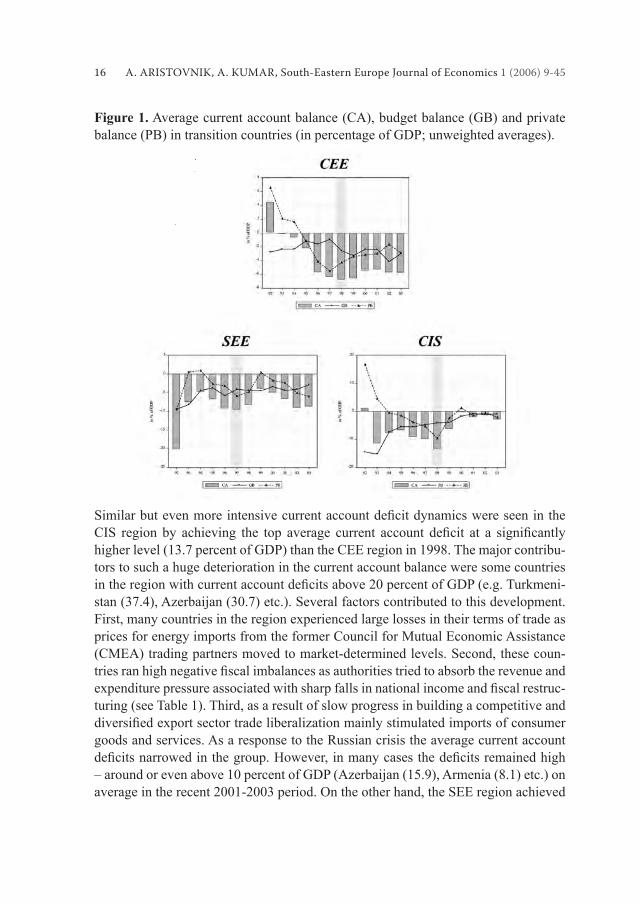
Table 1. Saving/Investment Imbalances in Transition Countries (in percentage of GDP; unweighted averages)
Sources: WDI (2004), EIU (2004), EBRD (2004), own calculations.
18 A. ARISTOVNIK, A. KUMAR, South-Eastern Europe Journal of Economics 1 (2006) 9-45
Development of investment and saving rates in transition countries
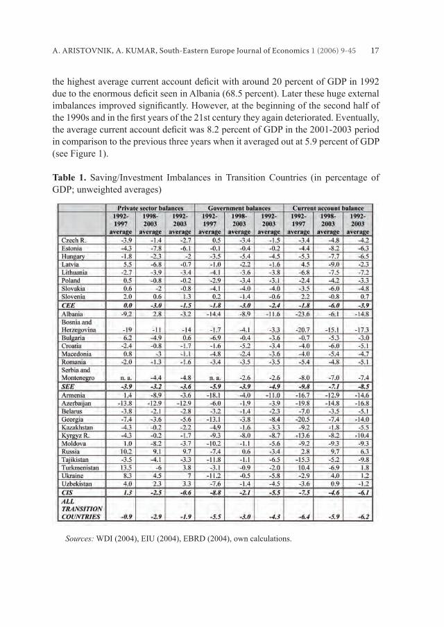
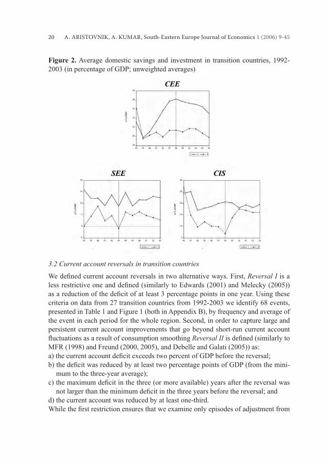
At the start of the transition more than a decade ago the investment-to-GDP ratio in all transition countries practically bottomed out in line with the drop in output (see Figure 2). Moreover, much of the capital stock at that time became obsolete over-night. Afterwards, investment rebounded, particularly in the CEE region (an aver-age of some 28 percent of GDP in 1998), when economies fought to transform their economies into market-oriented ones. Nevertheless, the rise in total investment in most transition countries during the 1990s was largely concentrated in the business sector. In fact, in most transition countries average government capital expenditure was less than 5 percent of GDP in the period. However, as part of the process of real convergence the investment ratio, also including public investment, may have to rise further to maintain strong economic growth. The various structural reforms being undertaken in transition countries should lead to an increase in the marginal productivity of domestic investment. Consequent-ly, the further reform of financial markets, particularly in the SEE and CIS regions,with respective investment rates of only around 13 and 18 percent of GDP in the 2001-2003 period, are needed to ensure efficient and productive capital allocation.Moreover, in order to spur growth potential and boost the capacity to service future debt repayments in transition countries, external borrowing for investment purposes is preferred to borrowing for consumption purposes. In this respect, capital inflows,in particular FDI, have been crucial in supporting these countries’ stronger invest-ment needs. In fact, for transition countries it may be best to attract foreign savings and direct them to productive investment. Data suggest that CEE has been the most successful region with its net FDI averaging out at almost 5 percent of GDP, whereas the CIS region attracted a net FDI of just above 4 percent of GDP on average in the 1992-2003 period.8 These figures are much higher than in developed countries, espe-cially in the EU-15, which averaged less than 3 percent of GDP in the same period. In most transition countries, during the pre-transition era domestic saving rates were exceptionally high. At the end of the 1980s the average saving rates of CEE, SEE and CIS were 32.9, 30.7 and 28.8 percent of GDP, respectively. These numbers are relatively high, especially given the EU-15 member states’ average saving rate of only some 20 percent of GDP in the same period.9 However, saving rates within the
8. Indeed, all three countries (Czech R., Slovakia and Poland) were confronted with a significantGDP slowdown in the following years. Eventually, when comparing annual GDP growth in the year before switching the exchange rate regime with the following three-year average, Czech R, Slovakia and Poland demonstrated a GDP growth decline of 3.5, 2.0 and 1.8 percentage points, respectively.9. In the 2000-2003 period the economies most attractive to FDI in the CEE region were Slovakia and Czech Republic with an average net FDI of 8.8 and 8.5 percent of GDP, respectively. In the CIS region, the biggest attractions are Azerbaijan and Kazakhstan with an average of 13.6 and 9.1 percent of GDP, respectively, in the same period.
A. ARISTOVNIK, A. KUMAR, South-Eastern Europe Journal of Economics 1 (2006) 9-45 19
transition economies differed widely, with Poland on top (42.7 percent) in 1989 and Tajikistan (12.5) and Kyrgyz Republic (13.1) at the bottom. Denizer and Wolf (2000) revealed three main factors which affected savings in the pre-transition era: first therewere ‘planned’ savings for funding ‘centrally planned’ investment. Second, the lack of consumer goods exposed limits on consumption below the desired levels and con-sequently induced so-called ‘involuntary savings’. Third, savings that were voluntary but driven by expectations of a systemic change, e.g. reflecting expectations of thegreater availability of goods. With the start of the transition process, the drop in domestic saving rates was enormous. Schrooten and Stephan (2003) pointed out at least three important factors which should be taken into account: consumption constraint, the savings overhang inherited from the past, and the massive uncertainty at the beginning of the transition process (high inflation, high unemployment, GDP decline etc.). However, a relativelyslow recovery has been observed despite huge differences both between and within the group of transition countries. For example, saving rates in CEE have stabilized at around 20 percent of GDP (the highest in the Czech Republic with around 26 percent, the lowest in Poland with around 15 percent) on average in recent years. On the other hand, in spite of significant saving rates improvements in CIS since 1998, they haverecently remained quite low, at around 17 percent of GDP (the highest in Russia with around 32 percent, the lowest in Moldova with even a negative savings rate of around 12 percent).10
A decomposition of the external imbalance between savings and investment shows that the main determinant of growing current account deficits has been, ingeneral, a remarkable increase in the average investment rate in CEE and a signifi-cant decline in the average saving rate in SEE and CIS in the 1992-2003 period.11 Indeed, the trends presented above mainly suggest an intertemporal approach to the current account, where transition countries (in particular CEE) use foreign savings to cushion their consumption in the face of unusually high investment needs. Moreo-ver, consumption smoothing in the intertemporal approach to the current account predicts a lower saving rate as private agents increase their consumption today based on expectations of a higher income in the future. In the case of transition countries, in particular in the latter stages of the transition process, the recent liberalization of financial markets and steadily improving access to credit by the domestic private sec-tor might be confronted with a declining saving rate as uncertainty becomes reduced and liquidity constraints are eased.12
10. The EU-15 average savings rate has remained stable at around 20 percent of GDP since then. 11. Due to data deficiencies it is hard to estimate a reliable level of the saving rate for the SEEregion. Nevertheless, according to the available data almost all economies in the region have rela-tively low or even negative saving rates.12. In fact, international comparisons (see MFR, 1996) suggest that low and falling saving rates make current account deficits less sustainable and potentially make the economy fragile.
20 A. ARISTOVNIK, A. KUMAR, South-Eastern Europe Journal of Economics 1 (2006) 9-45
Figure 2. Average domestic savings and investment in transition countries, 1992-2003 (in percentage of GDP; unweighted averages)
3.2 Current account reversals in transition countries
We defined current account reversals in two alternative ways. First, Reversal I is a less restrictive one and defined (similarly to Edwards (2001) and Melecky (2005))as a reduction of the deficit of at least 3 percentage points in one year. Using thesecriteria on data from 27 transition countries from 1992-2003 we identify 68 events, presented in Table 1 and Figure 1 (both in Appendix B), by frequency and average of the event in each period for the whole region. Second, in order to capture large and persistent current account improvements that go beyond short-run current account fluctuations as a result of consumption smoothing Reversal II is defined (similarly toMFR (1998) and Freund (2000, 2005), and Debelle and Galati (2005)) as:a) the current account deficit exceeds two percent of GDP before the reversal;b) the deficit was reduced by at least two percentage points of GDP (from the mini-
mum to the three-year average);c) the maximum deficit in the three (or more available) years after the reversal was
not larger than the minimum deficit in the three years before the reversal; andd) the current account was reduced by at least one-third.While the first restriction ensures that we examine only episodes of adjustment from
A. ARISTOVNIK, A. KUMAR, South-Eastern Europe Journal of Economics 1 (2006) 9-45 21
a current account deficit, the second and third ones ensure that there was a sustainedimprovement in the current account balances rather than sharp but temporary revers-als. The last restriction ensures that small improvements in very large current account deficits will not be considered as an adjustment (e.g. from 15 to 12 percent). As pre-sented in Table 1 and Figure 1 (Appendix B) we identify ten episodes of an (Reversal II) adjustment with CA/GDP ratio minimums concentrated between the 1997-2000 period. Moreover, for the complete transition region the incidence of Reversal I was 22.2 percent of all country-year observations, while it was just 3.3 percent for the Reversal II definition. The lowest incidence of reversals occurred in the advancedtransition economies (CEE) with only around 13 percent and in SEE with 2.5 percent for Reversals I and II, respectively. The region with the highest number of incidences is the CIS region with 27.6 percent and 3.7 percent, respectively. 3.3 Dynamics of the current account adjustment process
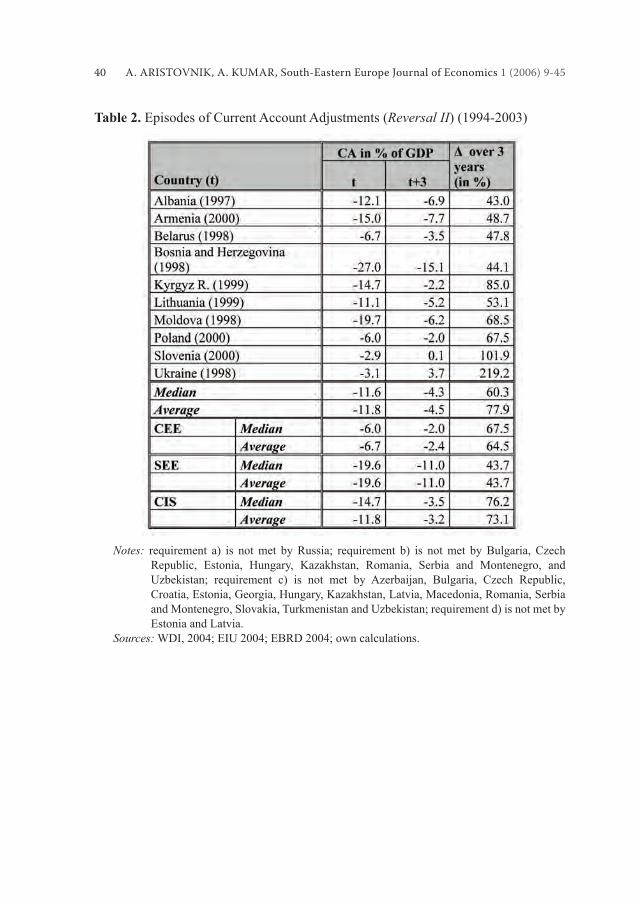
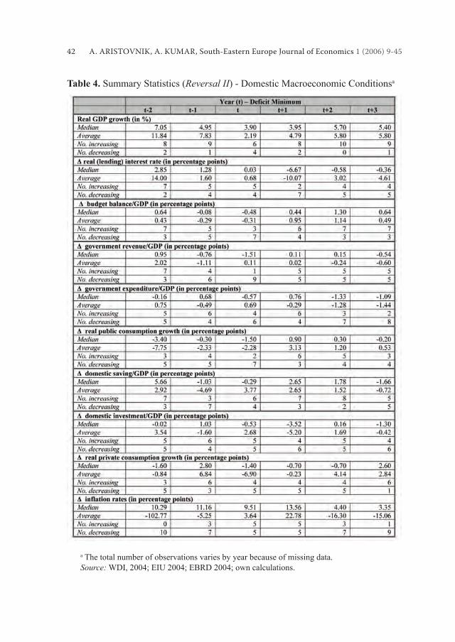
First, to study the adjustment process we focused on ten episodes of Reversals II among transition countries. In order to examine external adjustment process in transi-tion countries, we use different domestic internal and external macroeconomic aggre-gates such as real GDP growth, budget balance, savings, investments, the exchange rate, trade balance, external debt, international reserves and net international invest-ment position. The tabular (Table 4 and 5, Appendix B) and graphical evidence (Fig-ure 2-5, Appendix B) reveals several interesting findings on the behavior of currentaccount and macroeconomic variables during the ten episodes, which are discussed below. Current Account Balance: Figure 2 (in Appendix B) depicts the median and aver-age CA/GDP ratio for all ten transition countries under consideration and shows that the CA/GDP ratio continued to worsen at least 3 years before it hit its minimum and then jumped substantially in the first year of the reversal by around 8.5 percentagepoints on average. Afterwards, the adjustment process includes a gradual worsening of the current account balance in practically all the countries. In a typical case, the current account deficit reached almost 12 percent of GDP when it hit its minimum.However, the magnitude of the deficit/GDP ratio before the adjustment varies sub-stantially between regions (the lowest deficit was found in the CEE region with about6 percent of GDP; the highest was seen in the SEE region with almost 20 percent of GDP) as well as between countries (from 27 percent in Bosnia and Herzegovina (1998) to 2.9 percent in Slovenia (2000)).13 Similarly, the relative improvements of
13. Rodrik (2000) estimated that a 1-percentage point increase in the private-credit-to-income ratio would lower the long-term private saving rate by 0.74 of a percentage point in five CEE econo-mies.
22 A. ARISTOVNIK, A. KUMAR, South-Eastern Europe Journal of Economics 1 (2006) 9-45
current account balance in three years vary between 43 percent in Albania to around 220 percent in Ukraine (see Table 2 and Figure 2, Appendix B). Real GDP Growth: Analysis shows that the average and median real GDP growth peaks about two years before the deficit reaches its trough and is lowest when thedeficit bottoms out. In contrast to previous findings (e.g. Freund (2000), Freund andWarnock (2005), Melecky (2005) etc.) where in the typical case the annual real in-come hit its trough in the first year the current account improved, income growth intransition countries reaches its trough simultaneously with current account deficitsof more than 2 percent on average. Indeed, if we take into consideration the five-year period around the deficit minimum, only Poland and Slovenia reach their GDPgrowth minimum in the first or second year of their recovery. Moreover, annual realGDP growth was around 5 percent or even more before the trough of the current ac-count balance and then slowed down to around 2 percent in the year of the deficit’strough. Latter, however, the growth returned and stabilized between 5 and 6 percent annually, on average (see Figure 3, Appendix B). While in most countries GDP slow-down is seen in the pre-reversal period, we can assume that the GDP growth can have some predictive power for the reversal episode. Section 4 discusses this phenomenon in more detail. Budget Balance: As expected, the deterioration of the current account balance was associated with an expansion of the budget balance. However, not surprisingly, in the recovery period strong fiscal consolidation took place in the economies.14 In the typical case there was a budget deficit between 4 and 6 percent of GDP in the yearthe current CA/GDP ratio bottomed out. As GDP growth has returned and stabilized, most countries have experienced improvements in their budget balances. These de-velopments confirm the results of Aristovnik (2005) who claims that a 1 percentage point increase in the government budget deficit is associated on average with a 0.42of a percentage point increase in the current account deficit-to-GDP ratio, with eve-rything else being equal. The estimated coefficient also suggests that in transitioncountries private savings provide a significant but not a complete Ricardian offsetto changes in public saving. In fact, as a ratio to GDP, increases in private saving by about 0.6 of a percentage point are expected when the ratio of government saving to GDP decreases by 1 percentage point.15
14. Evidence for developed countries showed (see Mann (1999), Freund (2000) and Chinn and Prasad (2003)) that, on average, the current account tended to adjust when it approached levels of around 4-5 percent of GDP.15. Indeed, Calvo (2003) argues that reversals are strongly associated with the fiscal system andits institutions. Moreover, he emphasizes that lowering the fiscal deficit is highly effective in themedium term yet it could be counterproductive in the short run if it relies on higher taxes.
A. ARISTOVNIK, A. KUMAR, South-Eastern Europe Journal of Economics 1 (2006) 9-45 23
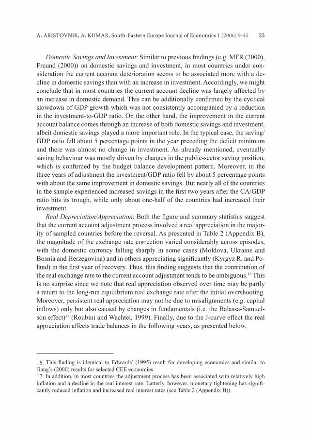
Domestic Savings and Investment: Similar to previous findings (e.g. MFR (2000),Freund (2000)) on domestic savings and investment, in most countries under con-sideration the current account deterioration seems to be associated more with a de-cline in domestic savings than with an increase in investment. Accordingly, we might conclude that in most countries the current account decline was largely affected by an increase in domestic demand. This can be additionally confirmed by the cyclicalslowdown of GDP growth which was not consistently accompanied by a reduction in the investment-to-GDP ratio. On the other hand, the improvement in the current account balance comes through an increase of both domestic savings and investment, albeit domestic savings played a more important role. In the typical case, the saving/GDP ratio fell about 5 percentage points in the year preceding the deficit minimumand there was almost no change in investment. As already mentioned, eventually saving behaviour was mostly driven by changes in the public-sector saving position, which is confirmed by the budget balance development pattern. Moreover, in thethree years of adjustment the investment/GDP ratio fell by about 5 percentage points with about the same improvement in domestic savings. But nearly all of the countries in the sample experienced increased savings in the first two years after the CA/GDPratio hits its trough, while only about one-half of the countries had increased their investment. Real Depreciation/Appreciation: Both the figure and summary statistics suggestthat the current account adjustment process involved a real appreciation in the major-ity of sampled countries before the reversal. As presented in Table 2 (Appendix B), the magnitude of the exchange rate correction varied considerably across episodes, with the domestic currency falling sharply in some cases (Moldova, Ukraine and Bosnia and Herzegovina) and in others appreciating significantly (Kyrgyz R. and Po-land) in the first year of recovery. Thus, this finding suggests that the contribution ofthe real exchange rate to the current account adjustment tends to be ambiguous.16 This is no surprise since we note that real appreciation observed over time may be partly a return to the long-run equilibrium real exchange rate after the initial overshooting. Moreover, persistent real appreciation may not be due to misalignments (e.g. capital inflows) only but also caused by changes in fundamentals (i.e. the Balassa-Samuel-son effect)17 (Roubini and Wachtel, 1999). Finally, due to the J-curve effect the real appreciation affects trade balances in the following years, as presented below.
16. This finding is identical to Edwards’ (1995) result for developing economies and similar toJiang’s (2000) results for selected CEE economies.17. In addition, in most countries the adjustment process has been associated with relatively high inflation and a decline in the real interest rate. Latterly, however, monetary tightening has signifi-cantly reduced inflation and increased real interest rates (see Table 2 (Appendix B)).
24 A. ARISTOVNIK, A. KUMAR, South-Eastern Europe Journal of Economics 1 (2006) 9-45
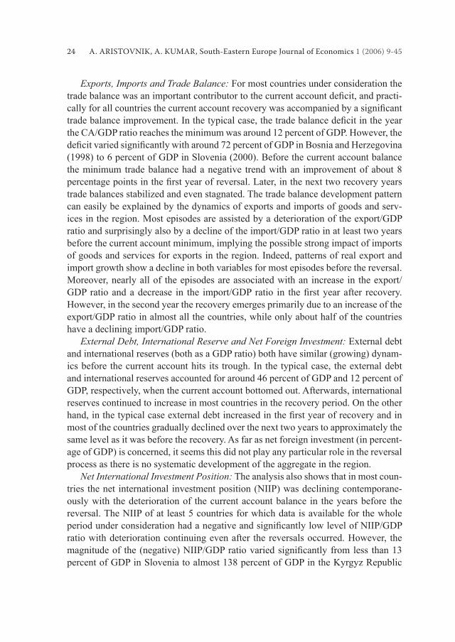
Exports, Imports and Trade Balance: For most countries under consideration the trade balance was an important contributor to the current account deficit, and practi-cally for all countries the current account recovery was accompanied by a significanttrade balance improvement. In the typical case, the trade balance deficit in the yearthe CA/GDP ratio reaches the minimum was around 12 percent of GDP. However, the deficit varied significantly with around 72 percent of GDP in Bosnia and Herzegovina(1998) to 6 percent of GDP in Slovenia (2000). Before the current account balance the minimum trade balance had a negative trend with an improvement of about 8 percentage points in the first year of reversal. Later, in the next two recovery yearstrade balances stabilized and even stagnated. The trade balance development pattern can easily be explained by the dynamics of exports and imports of goods and serv-ices in the region. Most episodes are assisted by a deterioration of the export/GDP ratio and surprisingly also by a decline of the import/GDP ratio in at least two years before the current account minimum, implying the possible strong impact of imports of goods and services for exports in the region. Indeed, patterns of real export and import growth show a decline in both variables for most episodes before the reversal. Moreover, nearly all of the episodes are associated with an increase in the export/GDP ratio and a decrease in the import/GDP ratio in the first year after recovery.However, in the second year the recovery emerges primarily due to an increase of the export/GDP ratio in almost all the countries, while only about half of the countries have a declining import/GDP ratio. External Debt, International Reserve and Net Foreign Investment: External debt and international reserves (both as a GDP ratio) both have similar (growing) dynam-ics before the current account hits its trough. In the typical case, the external debt and international reserves accounted for around 46 percent of GDP and 12 percent of GDP, respectively, when the current account bottomed out. Afterwards, international reserves continued to increase in most countries in the recovery period. On the other hand, in the typical case external debt increased in the first year of recovery and inmost of the countries gradually declined over the next two years to approximately the same level as it was before the recovery. As far as net foreign investment (in percent-age of GDP) is concerned, it seems this did not play any particular role in the reversal process as there is no systematic development of the aggregate in the region. Net International Investment Position: The analysis also shows that in most coun-tries the net international investment position (NIIP) was declining contemporane-ously with the deterioration of the current account balance in the years before the reversal. The NIIP of at least 5 countries for which data is available for the whole period under consideration had a negative and significantly low level of NIIP/GDPratio with deterioration continuing even after the reversals occurred. However, the magnitude of the (negative) NIIP/GDP ratio varied significantly from less than 13percent of GDP in Slovenia to almost 138 percent of GDP in the Kyrgyz Republic
A. ARISTOVNIK, A. KUMAR, South-Eastern Europe Journal of Economics 1 (2006) 9-45 25
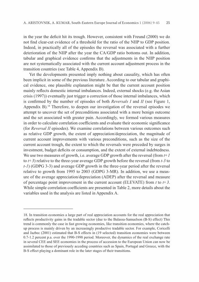
in the year the deficit hit its trough. However, consistent with Freund (2000) we donot find clear-cut evidence of a threshold for the ratio of the NIIP to GDP position. Indeed, in practically all of the episodes the reversal was associated with a further deterioration of the NIIP after the year the CA/GDP ratio bottoms out. In addition, tabular and graphical evidence confirms that the adjustments in the NIIP positionare not systematically associated with the current account adjustment process in the transition countries (see Table 4, Appendix B). Yet the developments presented imply nothing about causality, which has often been implicit in some of the previous literature. According to our tabular and graphi-cal evidence, one plausible explanation might be that the current account position mainly reflects domestic internal imbalances. Indeed, external shocks (e.g. the Asiancrisis (1997)) eventually just trigger a correction of those internal imbalances, which is confirmed by the number of episodes of both Reversals I and II (see Figure 1, Appendix B).18 Therefore, to deepen our investigation of the reversal episodes we attempt to uncover the set of preconditions associated with a more benign outcome and the set associated with greater pain. Accordingly, we formed various measures in order to calculate correlation coefficients and evaluate their economic significance(for Reversal II episodes). We examine correlations between various outcomes such as relative GDP growth, the extent of appreciation/depreciation, the magnitude of current account improvements with various preconditions, such as the size of the current account trough, the extent to which the reversals were preceded by surges in investment, budget deficits or consumption, and the extent of external indebtedness.We use two measures of growth, i.e. average GDP growth after the reversal (from t+1 to t+3) relative to the three-year average GDP growth before the reversal (from t-3 to t-1) (GDPG 3-3) and average GDP growth in the three-year period after the reversal relative to growth from 1995 to 2003 (GDPG 3-MR). In addition, we use a meas-ure of the average appreciation/depreciation (ADEP) after the reversal and measure of percentage point improvement in the current account (ELEVATE) from t to t+3. While simple correlation coefficients are presented in Table 2, more details about thevariables used in the analysis are listed in Appendix A.
18. In transition economies a large part of real appreciation accounts for the real appreciation that reflects productivity gains in the tradable sector (due to the Balassa-Samuelson (B-S) effect) Thistrend is commonly the case in fast growing economies, like transition economies, where the catch-up process is mainly driven by an increasingly productive tradable sector. For example, Coricelli and Jazbec (2001) estimated that B-S effects in (19 selected) transition economies were between 0.7-1.2 percent p.a. over the 1990-1998 period. Moreover, the dynamics of the real exchange rate in several CEE and SEE economies in the process of accession to the European Union can now be assimilated to those of previously acceding countries such as Spain, Portugal and Greece, with the B-S effect playing a dominant role in the later stages of their transitions.
26 A. ARISTOVNIK, A. KUMAR, South-Eastern Europe Journal of Economics 1 (2006) 9-45
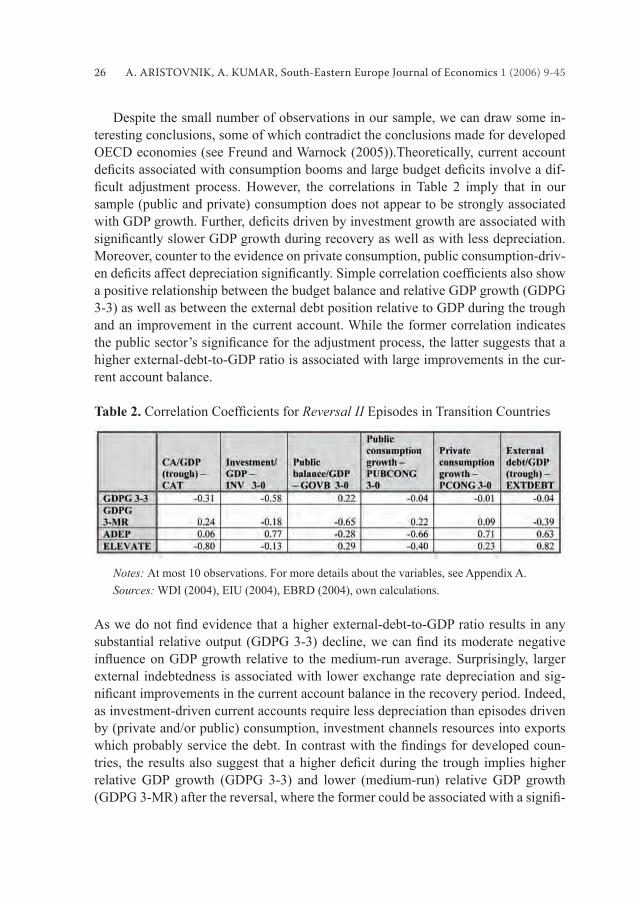
Despite the small number of observations in our sample, we can draw some in-teresting conclusions, some of which contradict the conclusions made for developed OECD economies (see Freund and Warnock (2005)).Theoretically, current account deficits associated with consumption booms and large budget deficits involve a dif-ficult adjustment process. However, the correlations in Table 2 imply that in oursample (public and private) consumption does not appear to be strongly associated with GDP growth. Further, deficits driven by investment growth are associated withsignificantly slower GDP growth during recovery as well as with less depreciation.Moreover, counter to the evidence on private consumption, public consumption-driv-en deficits affect depreciation significantly. Simple correlation coefficients also showa positive relationship between the budget balance and relative GDP growth (GDPG 3-3) as well as between the external debt position relative to GDP during the trough and an improvement in the current account. While the former correlation indicates the public sector’s significance for the adjustment process, the latter suggests that ahigher external-debt-to-GDP ratio is associated with large improvements in the cur-rent account balance.
Table 2. Correlation Coefficients for Reversal II Episodes in Transition Countries
Notes: At most 10 observations. For more details about the variables, see Appendix A. Sources: WDI (2004), EIU (2004), EBRD (2004), own calculations.
As we do not find evidence that a higher external-debt-to-GDP ratio results in anysubstantial relative output (GDPG 3-3) decline, we can find its moderate negativeinfluence on GDP growth relative to the medium-run average. Surprisingly, largerexternal indebtedness is associated with lower exchange rate depreciation and sig-nificant improvements in the current account balance in the recovery period. Indeed,as investment-driven current accounts require less depreciation than episodes driven by (private and/or public) consumption, investment channels resources into exports which probably service the debt. In contrast with the findings for developed coun-tries, the results also suggest that a higher deficit during the trough implies higherrelative GDP growth (GDPG 3-3) and lower (medium-run) relative GDP growth (GDPG 3-MR) after the reversal, where the former could be associated with a signifi-
A. ARISTOVNIK, A. KUMAR, South-Eastern Europe Journal of Economics 1 (2006) 9-45 27
cant deterioration of GDP growth during the period when the deficit is worsening.19 Moreover, a higher current account at the minimum implies a (negligible) exchange rate depreciation in the recovery period. Finally, the results also show that current account deficits are 80 percent reversed after three years, which is about the same asfor industrial countries (see Freund and Warnock, 2005).
3.4 Current account deficit persistency in transition countries
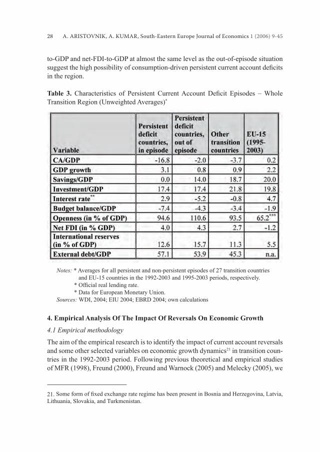
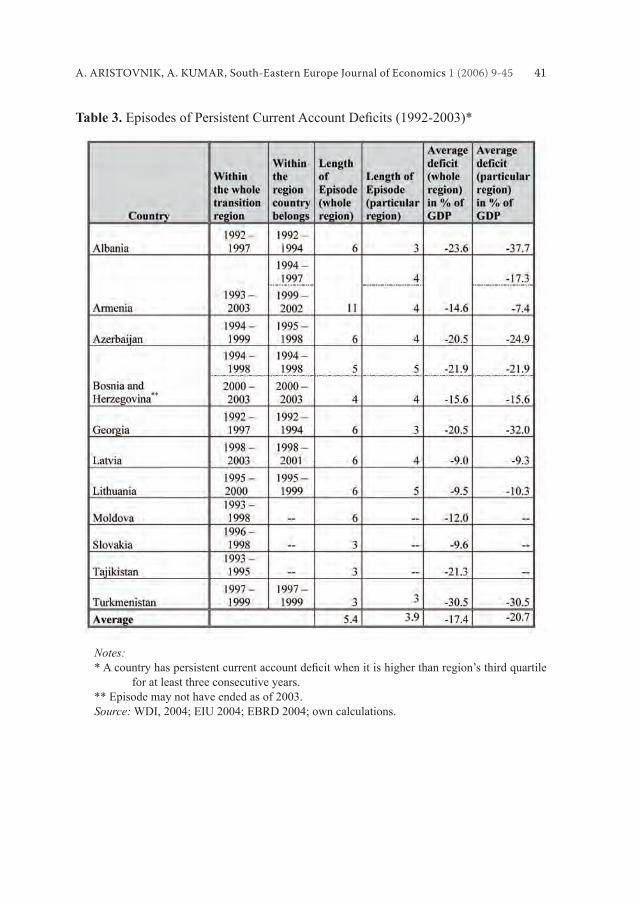
In addition to reversals, we briefly investigate the persistency of current account defi-cits which could be, according to Section 3, quite a common event in the region. We define deficit as persistent (similar to Edwards (2004)) if the current-account-deficit-to-GDP ratio is higher than the region’s third quartile for at least three consecutive years. As is seen in Table 3 in Appendix B, a relatively large number of countries has experienced periods of high and persistent deficits. Indeed, we identify twelve epi-sodes of persistent deficits in 11 countries when taking into account the whole transi-tion region and ten episodes in 8 countries when considering a particular transition region (CEE, SEE and CIS), whereas five episodes coincide with the reversal event(Albania, Armenia, Bosnia and Herzegovina, Lithuania and Moldova) (see Tables 2 and 3, Appendix B). According to arbitrarily defined persistency and considering thewhole transition region, the average current account deficit reaches around 17 percentof GDP and the average duration of a persistent episode is more than five years. By analyzing and comparing persistent deficits (in episodes) with the current ac-count deficits outside the episodes and also with all other transition countries as wellas EU-15 countries, more or less expected results can be observed (see Table 3). By definition, the current account position in the time horizons of a persistent deficit ison average extremely poor in comparisons with the out-of-episode period and with those countries that have not run persistent deficits. Moreover, key characteristicsinclude lower than average and even zero savings rates, somewhat elevated positive real interest rates, a higher budget deficit and gross external debt. They are also some-what more open, even though this measure is highly variable and does not account for country size. Moreover, the higher level of international reserves in countries with persistent (out-of-episode) deficits in comparison with other transition countiesmay be the result of the frequent use of some form of fixed exchange rate regimes inthe former countries.20 Finally, significantly higher GDP growth with investments-
19. Indeed, Edwards (2004) calculated that only around 29 percent of reversals in Eastern Europe coincided with ‘sudden stops’ of capital inflows and that around 43 percent of these ‘sudden stops’happened at the same time as reversals. Moreover, McGettigan (2000) set out internal factors (in particular a worsening of the fiscal situation) of the predicament of both countries.20. On the contrary, a simple regression between CA/GDP (trough) and GDP 3-3 for Reversal I epi-sodes reveals that a 1 percentage point higher deficit (in % of GDP) during a trough implies around(a statistically significant) 0.1 percentage point lower average relative GDP growth (GDP 3-3).
28 A. ARISTOVNIK, A. KUMAR, South-Eastern Europe Journal of Economics 1 (2006) 9-45
to-GDP and net-FDI-to-GDP at almost the same level as the out-of-episode situation suggest the high possibility of consumption-driven persistent current account deficitsin the region.
Table 3. Characteristics of Persistent Current Account Deficit Episodes – WholeTransition Region (Unweighted Averages)*
Notes: * Averages for all persistent and non-persistent episodes of 27 transition countries and EU-15 countries in the 1992-2003 and 1995-2003 periods, respectively. * Official real lending rate. * Data for European Monetary Union. Sources: WDI, 2004; EIU 2004; EBRD 2004; own calculations
4. Empirical Analysis Of The Impact Of Reversals On Economic Growth
4.1 Empirical methodology
The aim of the empirical research is to identify the impact of current account reversals and some other selected variables on economic growth dynamics21 in transition coun-tries in the 1992-2003 period. Following previous theoretical and empirical studies of MFR (1998), Freund (2000), Freund and Warnock (2005) and Melecky (2005), we
21. Some form of fixed exchange rate regime has been present in Bosnia and Herzegovina, Latvia, Lithuania, Slovakia, and Turkmenistan.
A. ARISTOVNIK, A. KUMAR, South-Eastern Europe Journal of Economics 1 (2006) 9-45 29
estimate a model which may be expressed in the following general form:
GDPGit = αi + γt + β’xit + εit ,
where the dependent variable is the percentage growth of real GDP (GDPG) for the i-th unit at time t and the vector of independent variables (xi) includes relative GDP, the investment rate, the government (public) balance, openness of the economy, external debt and impulse dummy variable accounting for reversals. αi represents individual effects which are specific to individual countries, the vector β’ is a vector of regres-sion coefficients, γt denotes time-specific effects which are peculiar to a particularperiod but constant for all countries while the error term εit represents the effects of the omitted variables that are peculiar to both the individual units and time periods. According to the previous theoretical and empirical considerations, we expect a negative relationship between the growth of real GDP and the (lagged) relative GDP level. In fact, countries with a higher GDP level tend to grow relatively slower. More-over, the variable may also be treated as a control for the cyclical part given the yearly frequency of observations. On the other hand, a positive effect is expected in the case of the investment rate as fixed capital formation should be an important impetus fordomestic income growth. Further, an increase of government sector savings would probably have a positive impact on GDP growth while the impact of the openness of the economy is likely to be ambiguous. On the contrary, theoretical and empirical literature suggests a strong negative sign for the reversal dummy variable in at least the first recovery year. However, with econometric analysis we seek to examine thefindings presented in the previous sections, i.e. that reversals in transition countriesare systematically associated with GDP growth slowdown, which would confirm up-to-date empirical results (e.g. Melecky (2005)).
4.2 Data
We estimate model (1) on the basis of pooled cross-sectional and time-series (panel) data for transition countries in the 1992-2003 period. The data set comes from the EBRD Transition Reports, the Economist Intelligence Unit (EIU), IMF International Financial Statistics (IFS) and Eurostat, and covers the 27 transition countries, i.e. eight CEE, seven SEE and twelve CIS countries with 68 Reversal I episodes. Our estimates are based on unbalanced panel data while for some countries included in the sample data were unavailable for the whole period. The dependent variable is the growth of real GDP (GDPG), expressed as a percentage. Independent variables are (lagged) relative GDP (RGDP) as measured by the ratio of a country’s actual GDP per capita and EU-15 GDP per capita (in PPS), the investment rate (INVEST) meas-ured as gross capital formation, the degree of openness (OPEN) measured as the sum of exports and imports of goods and services, government expenditure (GOVEXP)
(1)
30 A. ARISTOVNIK, A. KUMAR, South-Eastern Europe Journal of Economics 1 (2006) 9-45
and external debt (EXTDEBT), all expressed as a percentage of GDP. The final andmost important variable in our research, i.e. reversal (REV), is an impulse dummy variable measured with the value 1 for the year when the current account reaches the trough (t) and zeros otherwise. The empirical results are summarised in the next section where we estimate model (1) with the fixed-effect estimates (FEM), random-effect estimates (REM), estimates based on the feasible GLS method (FGLS) and panel corrected standard errors (OLS-PCSE). The results and tests are presented in Table 4.
4.3 Empirical Procedure
Since panel data typically exhibit group-wise heteroscedastic, contemporaneously and serially correlated residuals, we must take into account the existence of a non-spheri-cal error structure. As heterogeneity is the main characteristic of the countries under consideration, other specifications might be preferred to a simple OLS specificationin our analysis. In fact, in the case of transition countries this argument is plausible once differences like macroeconomic conditions and structural reforms are taken into account. First we run the FEM model and REM model specifications with countryeffects and also time effects. The Breusch-Pagan LM test confirms the appropriate-ness of the model based on panel data. Moreover, Hausman’s test indicates that for the model in the case of transition countries a random effect model (REM) provides a better specification. In order to ensure a higher degree of robustness of the estimateswe also employed two other methods: a revised Parks-Kmenta GLS method22 and the Beck-Katz PCSE method including country and time-specific effects. First, we applied a modified Wald test for group-wise heteroscedasticity to checkfor any common variance in the panels. Critical values of Chi-squared with 25 de-grees of freedom at a 1 percent significance level are 44.31, which are considerablylower than the test values obtained. Hence, we can reject the null hypothesis of ho-moscedasticity across the panels due to the different characteristics of the economies under consideration. Second, the contemporaneous or cross-sectional correlation is tested with the Breusch-Pagan LM test. According to the critical Chi-squared values a rejection of the null hypothesis of no cross-sectional correlation is possible. Third, the estimation rejects the null hypothesis of no serial correlation. In fact, critical val-ues of Chi-squared with 1 degree of freedom at 1 percent significance level are equalto 6.63. To sum up, the results of the tests presented above revealed that there is panel heteroscedasticity, cross-sectional correlation and a serial correlation of error terms
22. The forces governing long-run economic growth are presented in Barro and Sala-i-Martin (1995).
A. ARISTOVNIK, A. KUMAR, South-Eastern Europe Journal of Economics 1 (2006) 9-45 31
in the sample. Therefore, we follow Beck and Katz’s (1996) proposal that in the case of more countries than annual observations per economy, as in our group of transi-tion countries, the use of ordinary least squares with panel corrected standard errors (OLS-PCSE) is mostly preferred. However, Chen et al. (2005) suggest that use of the OLS-PCSE method is most appropriate if we are concentrating on testing hypotheses and the use of the FGLS method if our prime interest is accurate coefficient estimates.Therefore, we additionally ran the model by using the FGLS method in order to en-sure some degree of robustness.
4.4 Empirical Results
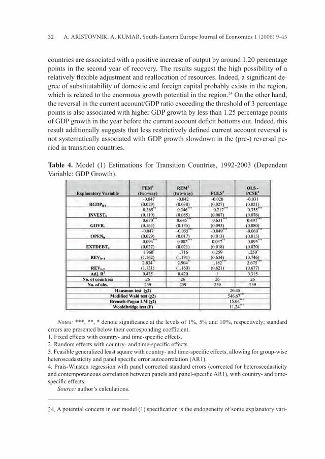
We now discuss the estimation results.23 The estimation results show that the conver-gence variable (relative lagged GDP) exhibits a correct but insignificant sign, whichprevents us confirming that countries with a higher GDP level tend to grow relativelyslower. Moreover, fixed capital accumulation is confirmed to be an important factorfor economic growth in the region. In fact, a significant positive coefficient suggeststhat a 1 percentage point increase in capital formation would elevate real GDP growth by 0.22 percentage points in the region. The results further imply that the general government sector balance (i.e. budget balance) has a strong positive impact on real GDP growth in transition countries. By reducing the public deficit by one percentagepoint, GDP growth would increase by almost two-thirds of a percentage point. This suggests that fiscal consolidation in the region with an additional reduction of publicdeficits should be one of the key factors of the further real convergence process. Theempirical results also imply there is a negative statistically significant relationshipbetween the openness of an economy and economic growth, albeit relatively negligi-ble. This result is inconsistent with a number of open-economy macroeconomic mod-els which postulate that the costs of foreign shocks (including reversals) are inversely proportional to the country’s degree of openness. However, another possible explana-tion here could be the large heterogeneity emerging due to the different development stages in the considered transition countries. Finally, the most important variable for our analysis, i.e. the impulse dummy vari-able for reversal, is included in the model. Exploring the dynamics of the reversals by leading and lagging the dummy variable, all except for the one-year leading and two-year lagging impulse dummy variables did not bring any statistically significantresults. Hence, we cannot statistically confirm any influence of reversals on the realGDP growth in the current (t) and subsequent year (t+1). Nevertheless, in accordance with the analyses in previous sections we calculated that the reversals in transition
23. The Parks-Kmenta method was revised by Beck and Katz (1996) who proposed the use of Fea-sible Generalized Least squares (FGLS) instead of GLS.
32 A. ARISTOVNIK, A. KUMAR, South-Eastern Europe Journal of Economics 1 (2006) 9-45
countries are associated with a positive increase of output by around 1.20 percentage points in the second year of recovery. The results suggest the high possibility of a relatively flexible adjustment and reallocation of resources. Indeed, a significant de-gree of substitutability of domestic and foreign capital probably exists in the region, which is related to the enormous growth potential in the region.24 On the other hand, the reversal in the current account/GDP ratio exceeding the threshold of 3 percentage points is also associated with higher GDP growth by less than 1.25 percentage points of GDP growth in the year before the current account deficit bottoms out. Indeed, thisresult additionally suggests that less restrictively defined current account reversal isnot systematically associated with GDP growth slowdown in the (pre-) reversal pe-riod in transition countries.
Table 4. Model (1) Estimations for Transition Countries, 1992-2003 (Dependent Variable: GDP Growth).
Notes: ***, **, * denote significance at the levels of 1%, 5% and 10%, respectively; standarderrors are presented below their corresponding coefficient.1. Fixed effects with country- and time-specific effects.2. Random effects with country- and time-specific effects.3. Feasible generalized least square with country- and time-specific effects, allowing for group-wiseheteroscedasticity and panel specific error autocorrelation (AR1).4. Prais-Winsten regression with panel corrected standard errors (corrected for heteroscedasticity and contemporaneous correlation between panels and panel-specific AR1), with country- and time-specific effects. Source: author’s calculations.
24. A potential concern in our model (1) specification is the endogeneity of some explanatory vari-
A. ARISTOVNIK, A. KUMAR, South-Eastern Europe Journal of Economics 1 (2006) 9-45 33
5. Conclusions
The paper has presented some characteristics of sharp reductions in current account deficits in transition countries. The analysis focuses on three important aspects ofthose current account reversals: a) to examine the factors that might have triggered the reversals and to provide some insights into the current account adjustment proc-ess; b) to reveal some characteristics of persistent current account deficits; and c) toexamine the direct impact of the reversals on economic growth in the region. The results of analyzing these issues reveal the following: a) When taking into account a restrictively defined reversal (Reversal II type), a typi-cal adjustment occurs when the current account deficit has grown for at least twoconsecutive years and reaches about 6 percent of GDP in CEE, 20 percent in SEE and 15 percent in CIS region. In the pre-reversal period the current account deterioration is likely to be associated with a deterioration in real GDP growth, domestic savings and export growth, as well as in the decreasing budget and trade balance. Accord-ingly, growing external debt and a declining net international investment position are no surprise in the years before the reversal of the current account. In the recovery pe-riod, however, reversals involve real GDP growth, a domestic savings increase and a decline in investment, substantial budget balance improvements, real export growth, an increase of international reserves and an eventual leveling off of the external debt. Nevertheless, the role of exchange rate depreciation in a typical current account re-versal episode seems to be ambiguous in the transition countries. Some deeper insights into the adjustment process suggest that deficits driven byinvestment growth are associated with significantly slower GDP growth during re-covery as well as with significantly less depreciation/higher appreciation in com-parisons with those episodes driven by private or public consumption. Moreover, (public) consumption-driven deficits increase exchange rate depreciation suggestingthe public sector’s high level of significance in the adjustment process. In contrastwith the findings for developed countries the results also suggest that a higher deficitduring a trough implies higher relative GDP growth after the reversal (in comparison with the pre-reversal period) and lower relative GDP growth (in comparison with the medium-run average). Finally, the results also show that current account deficits are80 percent reversed after three years, which is approximately the same as with indus-trial countries.
ables, reflected in correlation between these variables and error term causing biased and inconsist-ent estimates. According to Green (1997), one-year-lagged values of government expenditure are used as the instrument. Nevertheless, the results are principally supportive of the conclusions based on panel data estimates from Table 4.
34 A. ARISTOVNIK, A. KUMAR, South-Eastern Europe Journal of Economics 1 (2006) 9-45
b) The average persistent current account deficit reaches around 17 percent of GDPand the average duration of a persistent episode is more than five years. Moreover,the current account position in the time horizons of a persistent deficit is on averageextremely poor in comparisons with an out-of-episode period and with those transi-tion countries that have not run persistent deficits. In addition, key characteristicsinclude lower than average and even zero savings rates, somewhat elevated positive real interest rates, a higher budget deficit and gross external debt. Finally, the resultssuggest the high possibility of consumption-driven persistent current account deficitsin the region. c) The empirical investigation suggests that the reversal (Reversal I type) in the cur-rent account/GDP ratio exceeding the threshold of 3 percentage points is not sys-tematically associated with GDP growth slowdown in the years of the recovery. The empirical results might reflect the heterogeneity across episodes and are in a wayconsistent with the findings of Milesi-Ferretti and Razin (1998) for developing coun-tries. However, the results reveal that the reversals in the region are associated with GDP growing by less than 1.25 percentage point in the year before the current ac-count deficit bottoms out and with an increase of output by around 1.20 percentagepoints in the second year of recovery.
A. ARISTOVNIK, A. KUMAR, South-Eastern Europe Journal of Economics 1 (2006) 9-45 35
ReferencesAdalet, M., and Eichengreen, B., 2005, ‘Current Account Reversals: Always a Problem?’ NBER
Conference: G7 Current Account Imbalances: Sustainability and Adjustment, June 2005.Aristovnik, A., 2005, ‘Public Sector Stability and Balance of Payments Crises in Se-
lected Transition Economies.’ Democratic Governance for the XXI Century: Challenges and Responses in CEE Countries, May 2005.
Barro, Robert J. and Sala-i-Martin, X., 1995, Economic growth, Boston: McGraw-Hill, Mass.Beck, N., Katz, J. N., 1996, ‘Nuisance vs. substance: specifying and estimating time-series-cross
models.’ Political Analysis, Vol. 6: 1-36.Bussière, M., Fratzscher, M., and Müller G. J., 2004, ‘Current account dynamics in OECD and EU
acceding countries – an intertemporal approach.’ Frankfurt: EIB, Working Paper Series, No. 311.
Calvo, A. G., and Reinhart, C. M., 1999, ‘When Capital Inflows Come to a Sudden Stop: Conse-quences and Policy Options.’ Mimeo. University of Maryland.
Calvo, A.G., 2003, ‘Explaining Sudden Stops, Growth Collapse and BOP Crisis: The Case of Dis-tortionary Output Taxes.‘ IMF Staff Papers, Vol. 50, Special Issue.
Chen, X., Lin, S., and Reed, W.R., 2005, ‘Another Look At What To Do With Time-Series Cross-Section Data.’ Economics Working Paper Archive at WUSTL, No. 0506004
Chinn M., and Prasad, E. S., 2000, ‘Medium-term Determinants of Current Accounts in Industrial and Developing Countries: An Empirical Exploration’, NBER Working Paper, No. 7581.
Clarida, R., M. Goretti and M. Taylor, 2005, ‘Are There Thresholds of Current Account Adjust-ment?’ NBER Conference: G7 Current Account Imbalances: Sustainability and Adjustment, June 2005.
Coricelli, F., and Jazbec, B., 2001, ‘Real Exchange Rate Dynamics in Transition Economies.’ CEPR Discussion Papers, No. 2869.
Corsetti, G., Pensenti, P., and Roubini, N., 1998, ‘Paper Tigers? A Model of the Asian Crisis. ’ NBER Working Paper, No. 6783.
Croke, H., S. Kamin, and Leduc S., 2005, ‘Financial Market Developments and Economic Activity during Current Account Adjustments in Industrial Economies’ Federal Reserve Board, Interna-tional Finance Discussion Paper, No. 827.
Debelle, G. and Galati G., 2005, ‘Current Account Adjustment and Capital Flows.’ BIS Working Papers No. 169.
Denizer, C., and Wolf, H. C., 2000, ‘The Savings Collapse during the Transition in Eastern Europe.’ Washington: World Bank, Working Paper.
Edwards, S., 1995, ‘Why are Saving Rates So Different Across Countries?, An International Com-parative Analysis’, National Bureau of Economic Research, Cambridge, MA, NBER Working Paper, No. 5097.
Edwards, S., 2001, ‘Does the Current Account Matter?’, NBER Working Paper, No. 8275.Edwards, S., 2004, ‘Thirty Years of Current Account Imbalances’, Current Account Reversals and
Sudden Stops, NBER Working Paper, No. 10276.Fidrmuc, J., 2003, ‘The Feldstein-Horioka Puzzle and Twin Deficits in Selected Economies.’ Eco-
nomics of Planning, Vol. 36: 135-152.Fischer, S., 2003, ‘Financial Crisis and Reform of the International Financial System.’ Review of
World Economics/Weltwirtscahfliches Archiv, 139(1):1-37.Frankel, J., Rose A., 1996, ‘Currency crashes in emerging markets: an empirical treatment.’ Journal
of International Economics 41(3-4), 351-66.Freund, C., 2000, ‘Current Account Adjustment in Industrial Countries.’ International Finance Dis-
cussion Papers, No. 692.
36 A. ARISTOVNIK, A. KUMAR, South-Eastern Europe Journal of Economics 1 (2006) 9-45
Freund, C., and Warnock, F., 2005, ‘Current Account Deficits in Industrial Countries: The BiggerThey Are, The Harder They Fall?’ NBER Conference: G7 Current Account Imbalances: Sus-tainability and Adjustment, June 2005.
Greene William H., 1997, Econometric Analysis. New York, Prentice Hall, 1997.Kamin, S., Schindler, J., and Samuel, S., 2001, ‘The Contribution of Domestic and External Factors
to Emerging Market Devaluation Crises: An Early Warning Systems Approach’, International Finance Discussion Papers, No. 711.
Mann, C., 1999, ‘Is the US Trade Deficit Sustainable?’ Institute for International Economics. McGettigan, D., 2000, ‘Current Account and External Sustainability in the Baltics, Russia, and
Other Countries of the Former Soviet Union.’ IMF Occasional Paper, No. 189.Melecky, M., 2005, ‘The Impact of Current Account Reversals on Growth in Central and Eastern
Europe.’ Economics Working Paper Archive at WUSTL, No. 0502004.Milesi-Ferretti, G.M., Razin, A., 1996, ‘Sustainability of Persistent Current Account Deficits.’
NBER Working Paper, No. 5467.Milesi-Ferretti, G.M., Razin, A., 1998, ‘Current Account Reversals and Currency Crises: Empirical
Regularities.’ NBER Working Paper, No. 6620.Miller, N. C., 2002, Balance of Payments and Exchange Rate Theories. Cheltenham: Edward Elgar
Publishing Limited.Obstfeld, M., and Rogoff K., 1996, Foundations of International Macroeconomics, Cambridge,
MA: MIT Press. Radelet, S., and Sachs, J., 2000, ‘The Onset of the East Asian Currency Crisis.’ NBER Working
Paper, No. 6680.Rodrik, D., 2000, ‘Saving Transitions’. World Bank Economic Review, 14(3): 481-507.Roubini, N., and Wachtel, P., 1999, ‘Current-Account Sustainability in Transition Economies.’ Bal-
ance of Payments, Exchange Rates, and Competitiveness in Transition Economies, Kluwer Academic Publishers.
Schrooten, M., and Stephan, S., 2003, ‘Back on track? Savings Puzzles in EU-Accession Coun-tries.’ Berlin: German Institute for Economic Research. Discussion Papers of DIW Berlin, No. 306.
Summers, L. H., 2000, ‘International Financial Crises: Causes, Prevention, and Cures.’ American Economic Review, 90 (2).
Svejnar, J., 2002, ‘Transition Economies: Performance and Challenges.’ William Davidson Working Paper, No. 415.
Zanghieri, P., 2004, ‘Current Account Dynamics in New EU Members: Sustainability and Policy Issues.’ CEPII, Working Papers, 2004-07.
A. ARISTOVNIK, A. KUMAR, South-Eastern Europe Journal of Economics 1 (2006) 9-45 37
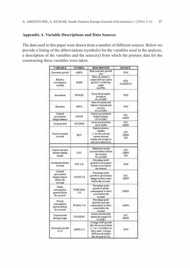
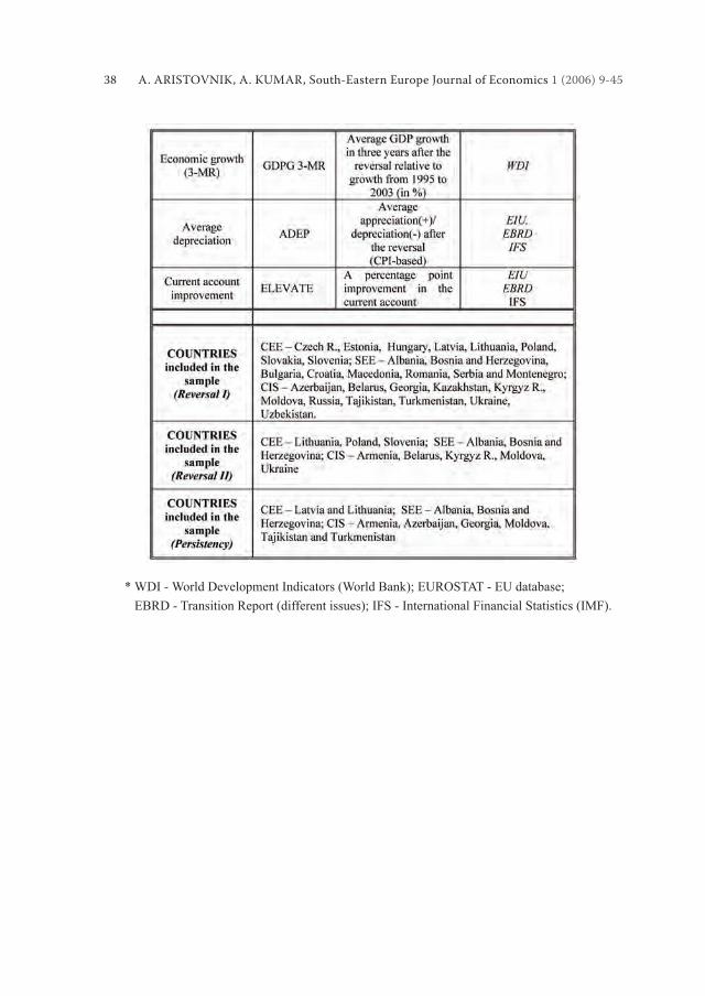
Appendix A. Variable Descriptions and Data Sources
The data used in this paper were drawn from a number of different sources. Below we provide a listing of the abbreviations (symbols) for the variables used in the analysis, a description of the variables and the source(s) from which the primary data for the constructing these variables were taken.
38 A. ARISTOVNIK, A. KUMAR, South-Eastern Europe Journal of Economics 1 (2006) 9-45
* WDI - World Development Indicators (World Bank); EUROSTAT - EU database; EBRD - Transition Report (different issues); IFS - International Financial Statistics (IMF).

A. ARISTOVNIK, A. KUMAR, South-Eastern Europe Journal of Economics 1 (2006) 9-45 39
Appendix B. Figures and Tables
Table 1. Current Account Reversals in Transition Countries (1992-2003)
Notes: *Russia’s current account reversals include significant improvements in the current account surplus, as well as in some cases in Turkmenistan and Ukraine. Sources: WDI, 2004; EIU 2004; EBRD 2004; own calculations.
40 A. ARISTOVNIK, A. KUMAR, South-Eastern Europe Journal of Economics 1 (2006) 9-45
Table 2. Episodes of Current Account Adjustments (Reversal II) (1994-2003)
Notes: requirement a) is not met by Russia; requirement b) is not met by Bulgaria, Czech Republic, Estonia, Hungary, Kazakhstan, Romania, Serbia and Montenegro, and Uzbekistan; requirement c) is not met by Azerbaijan, Bulgaria, Czech Republic, Croatia, Estonia, Georgia, Hungary, Kazakhstan, Latvia, Macedonia, Romania, Serbia and Montenegro, Slovakia, Turkmenistan and Uzbekistan; requirement d) is not met by Estonia and Latvia.
Sources: WDI, 2004; EIU 2004; EBRD 2004; own calculations.
A. ARISTOVNIK, A. KUMAR, South-Eastern Europe Journal of Economics 1 (2006) 9-45 41
Table 3. Episodes of Persistent Current Account Deficits (1992-2003)*
Notes: * A country has persistent current account deficit when it is higher than region’s third quartile
for at least three consecutive years. ** Episode may not have ended as of 2003. Source: WDI, 2004; EIU 2004; EBRD 2004; own calculations.
42 A. ARISTOVNIK, A. KUMAR, South-Eastern Europe Journal of Economics 1 (2006) 9-45
Table 4. Summary Statistics (Reversal II) - Domestic Macroeconomic Conditionsa
a The total number of observations varies by year because of missing data. Source: WDI, 2004; EIU 2004; EBRD 2004; own calculations.
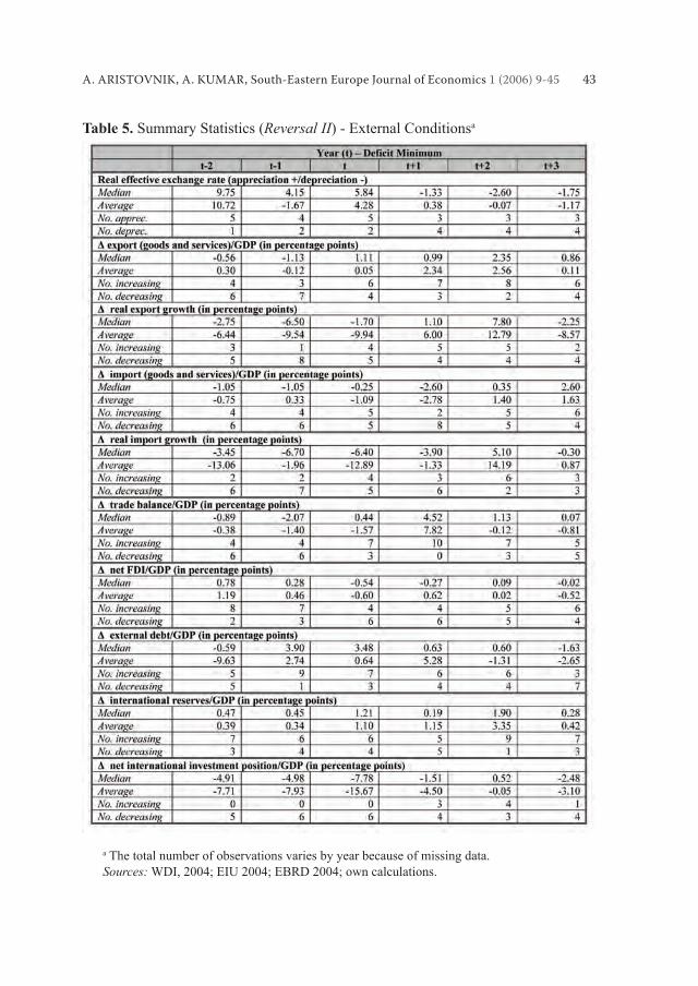
A. ARISTOVNIK, A. KUMAR, South-Eastern Europe Journal of Economics 1 (2006) 9-45 43
Table 5. Summary Statistics (Reversal II) - External Conditionsa
a The total number of observations varies by year because of missing data. Sources: WDI, 2004; EIU 2004; EBRD 2004; own calculations.
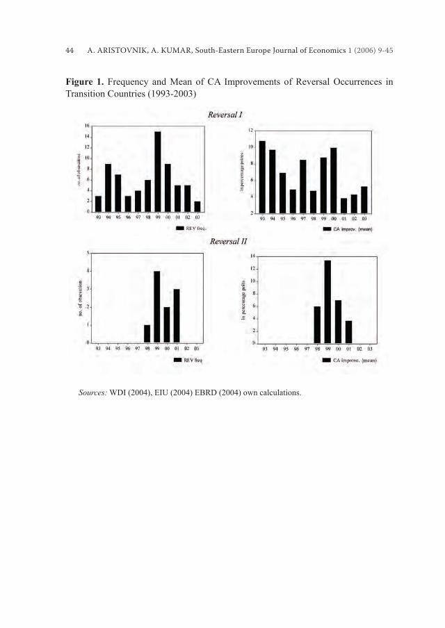
44 A. ARISTOVNIK, A. KUMAR, South-Eastern Europe Journal of Economics 1 (2006) 9-45
Figure 1. Frequency and Mean of CA Improvements of Reversal Occurrences in Transition Countries (1993-2003)
Sources: WDI (2004), EIU (2004) EBRD (2004) own calculations.
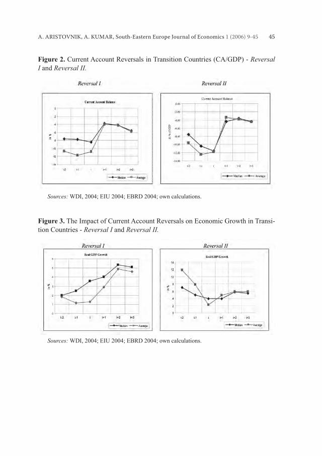
A. ARISTOVNIK, A. KUMAR, South-Eastern Europe Journal of Economics 1 (2006) 9-45 45
Figure 2. Current Account Reversals in Transition Countries (CA/GDP) - Reversal I and Reversal II.
Sources: WDI, 2004; EIU 2004; EBRD 2004; own calculations.
Figure 3. The Impact of Current Account Reversals on Economic Growth in Transi-tion Countries - Reversal I and Reversal II.
Sources: WDI, 2004; EIU 2004; EBRD 2004; own calculations.