thales-logo

1/1

Solving Sparse Systems with the BlockWiedemann Algorithm

E�cient Implementation over GF(2)

Sonia Belaid Sylvain Lachartre

Séminaire SALSA

2011, 8 July

grid

thales-logo

8/07/2011 2/1

Outline

grid

thales-logo

8/07/2011 3/1

Outline

grid

thales-logo

8/07/2011 4/1

Introduction

� Wiedemann's algorithm was introduced by Wiedemann in1986 [?]

� It was extended by Coppersmith in 1994 [?] to performparallel computations

� It was improved and used by Emmanuel Thomé [?] and aninternational team of researchers in 2009 to break a 768 bitsRSA key [?]

grid

thales-logo

8/07/2011 5/1

Scalar Wiedemann

� Input : large sparse matrix B

� Computation of the linearly recurrent sequence

xT · Bk · z

with x and z random vectors

� Computation of the minimal polynomial µ(X ) = X · µ′(X )(because B is singular) using Berlekamp-Massey

� Exhibition of the kernel vector v such that

v = µ′(B)

grid

thales-logo

8/07/2011 6/1

Outline

grid

thales-logo

8/07/2011 7/1

Outline

grid

thales-logo

8/07/2011 8/1

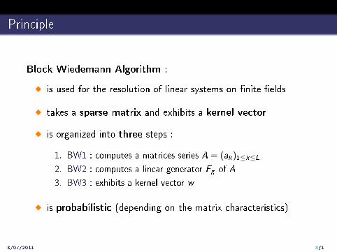
Principle

Block Wiedemann Algorithm :

� is used for the resolution of linear systems on �nite �elds

� takes a sparse matrix and exhibits a kernel vector

� is organized into three steps :

1. BW1 : computes a matrices series A = (ak)1≤k≤L

2. BW2 : computes a linear generator Fg of A

3. BW3 : exhibits a kernel vector w

� is probabilistic (depending on the matrix characteristics)

grid

thales-logo

8/07/2011 9/1

Main Algorithm

Algorithm 1 Wiedemann

Input: matrix B ∈ GF(2)N×N

Output: vector w ∈ GF(2)N

1. (A, z)← BW1(B) // z ∈ GF(2)N×n (random)

2. Fg ← BW2(A) // Fg ∈ GF(2)N (linear generator)

3. w ← BW3(Fg ,B,A, z)

4. return w

� Input : large sparse matrix B

� Output : kernel vector w

� N : input matrix dimension

� m,n : columns number of random blocks x and z

grid

thales-logo

8/07/2011 10/1

BW1 : Sequence A

� The �rst step consists in computing the series

A(X)← Σkak · X k with ak ← xT · Bk · z ∈ GF(2)m×n

� Only the �rst L = Nm + N

n + 1 coe�cients are needed

Algorithm 2 BW1

Input: matrix BOutput: polynomial A ∈ GF(2)[[X ]]m×n, matrix z ∈ GF(2)N×n

1. (x , z)← random matrices ∈ GF(2)N×m ×GF(2)N×n

2. v ← B · z3. for k ← 0 to L do

4. A[k] a← xT · v5. v ← B · v6. endfor

7. return A

a. A[k] represents the degree k coe�cient of A

grid

thales-logo

8/07/2011 11/1

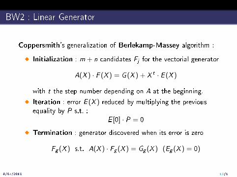
BW2 : Linear Generator

Coppersmith's generalization of Berlekamp-Massey algorithm :

� Initialization : m + n candidates Fj for the vectorial generator

A(X ) · F (X ) = G (X ) + X t · E (X )

with t the step number depending on A at the beginning.

� Iteration : error E (X ) reduced by multiplying the previousequality by P s.t. :

E [0] · P = 0

� Termination : generator discovered when its error is zero

Fg (X ) s.t. A(X ) · Fg (X ) = Gg (X ) (Eg (X ) = 0)

grid

thales-logo

8/07/2011 12/1

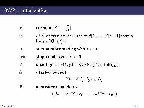
BW2 : Initialization

d constant d ← dNme

s F (t0) degree s.t. columns of A[0], . . . ,A[s − 1] form abasis of GF(2)m

t step number starting with t ← s

end stop condition end ← 0

δ quantity s.t. δ(f , g) = max(deg f , 1 + deg g)

∆ degrees bounds

∀j , δ(Fj ,Gj) ≤ ∆j

F generator candidates(In | X s−i1 · r1 . . . X s−im · rm

)

grid

thales-logo

8/07/2011 13/1

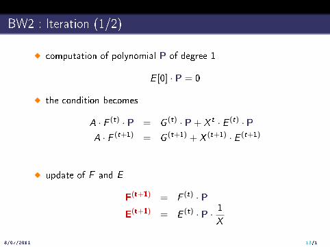
BW2 : Iteration (1/2)

� computation of polynomial P of degree 1

E [0] · P = 0

� the condition becomes

A · F (t) · P = G (t) · P + X t · E (t) · PA · F (t+1) = G (t+1) + X (t+1) · E (t+1)

� update of F and E

F(t+1) = F (t) · PE(t+1) = E (t) · P · 1

X

grid

thales-logo

8/07/2011 14/1

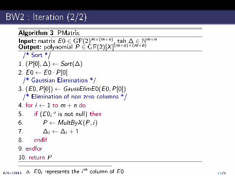
BW2 : Iteration (2/2)

Algorithm 3 PMatrix

Input: matrix E0 ∈ GF(2)m×(m+n), tab ∆ ∈ Nm+n

Output: polynomial P ∈ GF(2)[X ](m+n)×(m+n)

/* Sort */

1. (P[0],∆)← Sort(∆)

2. E0← E0 · P[0]/* Gaussian Elimination */

3. (E0,P[0])← GaussElimE0(E0,P[0])/* Elimination of non zero columns */

4. for i ← 1 to m + n do

5. if (E0ia is not null) then

6. P ← MultByX (P, i)

7. ∆i ← ∆i + 1

8. endif

9. endfor

10. return P

a. E0i represents the ith column of E0

grid

thales-logo

8/07/2011 15/1

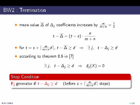
BW2 : Termination

� mean value ∆ of ∆j coe�cients increases by mm+n = 1

2

t −∆ = (t − s) · n

m + n

� for t = s + d mm+nde, t −∆ ≥ d ⇒ ∃ j , t −∆j ≥ d

� according to theorem 8.6 in [?]

∃ j , t −∆j ≥ d ⇒ Ej(X ) = 0

Stop Condition

Fj generator if t −∆j ≥ d (before s + d mm+nde steps)

grid

thales-logo

8/07/2011 16/1

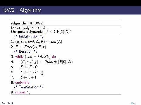
BW2 : Algorithm

Algorithm 4 BW2

Input: polynomial AOutput: polynomial F ∈ GF(2)[X ]n

/* Initialization */

1. (d , s, t, end ,∆,F )← Init(A)

2. E ← Error(A,F , t)/* Iteration */

3. while (end = FALSE ) do

4. (P, end , g)← PMatrix(E [0],∆)

5. F ← F · P6. E ← E · P · 1

X

7. t ← t + 1

8. endwhile/* Termination */

9. return Fg

grid

thales-logo

8/07/2011 17/1

BW3 : Kernel Vector

Kernel vector exhibition :

� coe�cient j of A(X ) · Fg (X )

(A·Fg )[j ] = xT ·B j−deg Fg+1·v with v =

deg Fg∑i=0

Bdeg Fg−i ·z ·Fg [i ]

� by construction

(A · Fg )[j ] = 0 for j ≥ δ(Fg )

� Bδ(F )−deg Fg+1 · v orthogonal to all vectors (BT )i · xk

� if these vectors form a basis of KN

B · (Bδ(Fg )−deg Fg · v︸ ︷︷ ︸Kernel Vector

) = 0

grid

thales-logo

8/07/2011 18/1

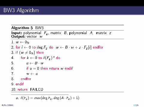
BW3 Algorithm

Algorithm 5 BW3

Input: polynomial Fg , matrix B, polynomial A, matrix zOutput: vector w

1. w ← 0N2. for i ← 0 to deg Fg do w ← B · w + z · Fg [i ] endfor

3. if (w 6= 0N) then

4. for k ← 0 to δ(Fg ) a do

5. u ← B · w6. if u = 0 then return w endif

7. w ← u

8. endfor

9. endif

10. return FAILED

a. δ(Fg ) = max(deg Fg , deg (A · Fg ) + 1)

grid

thales-logo

8/07/2011 19/1

Outline

grid

thales-logo

8/07/2011 20/1

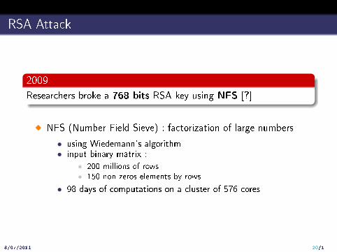
RSA Attack

2009

Researchers broke a 768 bits RSA key using NFS [?]

� NFS (Number Field Sieve) : factorization of large numbers

• using Wiedemann's algorithm• input binary matrix :

∗ 200 millions of rows∗ 150 non zeros elements by rows

• 98 days of computations on a cluster of 576 cores

grid

thales-logo

8/07/2011 21/1

Outline

grid

thales-logo

8/07/2011 22/1

Outline

grid

thales-logo

8/07/2011 23/1

Library M4RI [?]

� Linear algebra library in C language focused on dense matricesover GF(2)

� Created by Gregory Bard

� Now maintained by Martin Albrecht

� We use it to compute operations on dense matrices

• BW1 : to compute the products of x · (Bk · z)

• BW2 : to perform all the operations involving blocks

• BW3 : to compute the products (B · z) · F

grid

thales-logo

8/07/2011 24/1

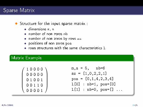
Sparse Matrix

� Structure for the input sparse matrix :

• dimensions m, n• number of non zeros nb• number of non zeros by rows sz• positions of non zeros pos• rows structures with the same characteristics l

Matrix Example1 0 0 0 00 0 0 0 00 1 0 0 10 0 1 1 00 0 0 0 1

m,n = 5, nb=6

sz = [1,0,2,2,1]

pos = [0,1,4,2,3,4]

l[0] : nb=1, pos=[0]

l[1] : nb=0, pos=[] ...

grid

thales-logo

8/07/2011 25/1

Sparse Dense Operations

Algorithm 6 Sparse Dense Product

Input: matrix B, matrix vOutput: matrix res ← B · v1. res ← 0

2. p ← Bpos

3. for i ← 0 to N do

4. for j ← 0 to Bi nb do

5. resi ← resi ⊕ vp

6. p ← p + 1

7. endfor

8. endfor

9. return res

� Complexity : linear with the number of non zeros.

grid

thales-logo

8/07/2011 26/1

Outline

grid

thales-logo

8/07/2011 27/1

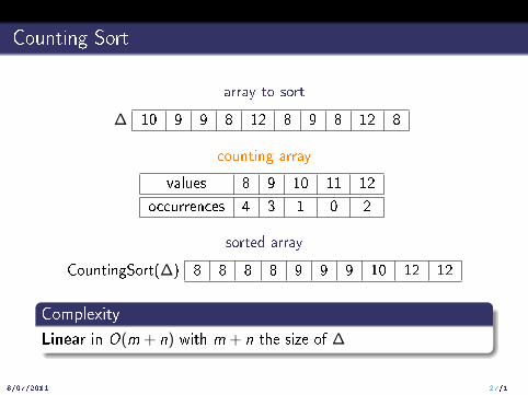
Counting Sort

array to sort

∆ 10 9 9 8 12 8 9 8 12 8

counting array

values 8 9 10 11 12

occurrences 4 3 1 0 2

sorted array

CountingSort(∆) 8 8 8 8 9 9 9 10 12 12

Complexity

Linear in O(m + n) with m + n the size of ∆

grid

thales-logo

8/07/2011 28/1

Outline

grid

thales-logo

8/07/2011 29/1

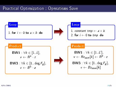
Practical Optimization : Operations Save

1. for i ← 0 to a× b do

Loop

1. constant tmp ← a× b

2. for i ← 0 to tmp do

Loop

BW1 : ∀k ∈ [1..L],v ← Bk · z

BW3 : ∀k ∈ [1.. deg Fg ],v ← Bk · z

Product

BW1 : ∀k ∈ [1..L′],v ← Bzsave [k]← Bk · z

BW3 : ∀k ∈ [1.. deg Fg ],v ← Bzsave [k]

Product

grid

thales-logo

8/07/2011 30/1

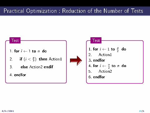
Practical Optimization : Reduction of the Number of Tests

1. for i ← 1 to n do

2. if (i < n2

) then Action1

3. else Action2 endif

4. endfor

Test

1. for i ← 1 to n2

do

2. Action1

3. endfor

4. for i ← n2to n do

5. Action2

6. endfor

Test

grid

thales-logo

8/07/2011 31/1

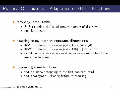
Practical Optimization : Adaptation of M4RI 1 Functions

� removing initial tests

• A · B : number of A's columns = number of B's rows• equality to zero

� adapting to my matrices constant dimensions

• BW1 : products of matrices (64× N)× (N × 64)• BW2 : products of matrices (64× 128)× (128× 128)• global : most matrices whose dimensions are multiples of the

size a machine word

� improving some functions

• mzd_is_zero : stopping at the �rst non zero word• mzd_transpose : clearing before transposing

1. released 2009-05-12

grid

thales-logo

8/07/2011 32/1

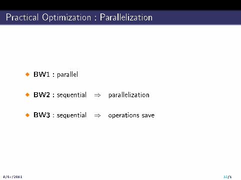
Practical Optimization : Parallelization

� BW1 : parallel

� BW2 : sequential ⇒ parallelization

� BW3 : sequential ⇒ operations save

grid

thales-logo

8/07/2011 33/1

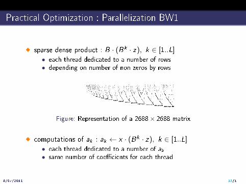
Practical Optimization : Parallelization BW1

� sparse dense product : B · (Bk · z), k ∈ [1..L]

• each thread dedicated to a number of rows• depending on number of non zeros by rows

Figure: Representation of a 2688× 2688 matrix

� computations of ak : ak ← x · (Bk · z), k ∈ [1..L]

• each thread dedicated to a number of ak• same number of coe�cients for each thread

grid

thales-logo

8/07/2011 34/1

Practical Optimization : Parallelization BW2

� polynomials products F · P and E · P• each thread dedicated to a number of coe�cients of F or E• same number of coe�cients for each thread

� product of P by X

• each thread dedicated to a number of columns of P• same number of columns for each thread

grid

thales-logo

8/07/2011 35/1

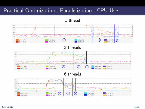
Practical Optimization : Parallelization : CPU Use

1 thread

3 threads

6 threads

grid

thales-logo

8/07/2011 36/1

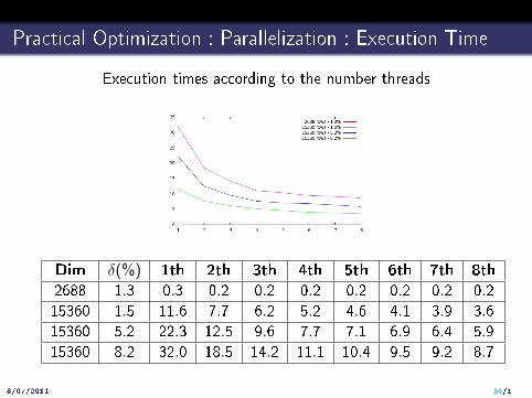
Practical Optimization : Parallelization : Execution Time

Execution times according to the number threads

Dim δ(%) 1th 2th 3th 4th 5th 6th 7th 8th

2688 1.3 0.3 0.2 0.2 0.2 0.2 0.2 0.2 0.2

15360 1.5 11.6 7.7 6.2 5.2 4.6 4.1 3.9 3.6

15360 5.2 22.3 12.5 9.6 7.7 7.1 6.9 6.4 5.9

15360 8.2 32.0 18.5 14.2 11.1 10.4 9.5 9.2 8.7

grid

thales-logo

8/07/2011 37/1

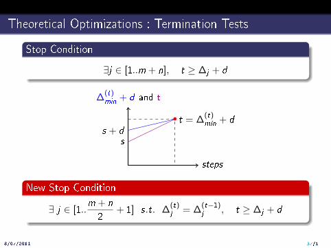
Theoretical Optimizations : Termination Tests

Stop Condition

∃j ∈ [1..m + n], t ≥ ∆j + d

∆(t)min + d and t

steps

ss + d

t = ∆(t)min + d

New Stop Condition

∃ j ∈ [1..m + n

2+ 1] s.t. ∆

(t)j = ∆

(t−1)j , t ≥ ∆j + d

grid

thales-logo

8/07/2011 38/1

Theoretical Optimizations : Error Degree Update (1/2)

� for large matrices

• high error degree in BW2

• product E · P expensive

� but only E[0] used in each step

� knowing the number of reminding steps, we can :

• determine the useful degree of E

• decrease the number of coe�cients to update

grid

thales-logo

8/07/2011 39/1

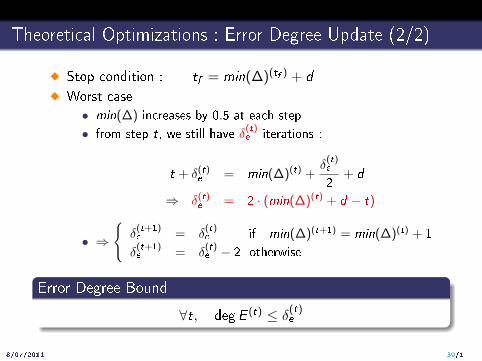
Theoretical Optimizations : Error Degree Update (2/2)

� Stop condition : tf = min(∆)(tf ) + d

� Worst case

• min(∆) increases by 0.5 at each step

• from step t, we still have δ(t)e iterations :

t + δ(t)e = min(∆)(t) +δ(t)e

2+ d

⇒ δ(t)e = 2 · (min(∆)(t) + d − t)

• ⇒

{δ(t+1)e = δ

(t)e if min(∆)(t+1) = min(∆)(t) + 1

δ(t+1)e = δ

(t)e − 2 otherwise

Error Degree Bound

∀t, deg E (t) ≤ δ(t)e

grid

thales-logo

8/07/2011 40/1

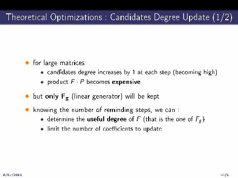
Theoretical Optimizations : Candidates Degree Update (1/2)

� for large matrices

• candidates degree increases by 1 at each step (becoming high)

• product F · P becomes expensive

� but only Fg (linear generator) will be kept

� knowing the number of reminding steps, we can :

• determine the useful degree of F (that is the one of Fg )

• limit the number of coe�cients to update

grid

thales-logo

8/07/2011 41/1

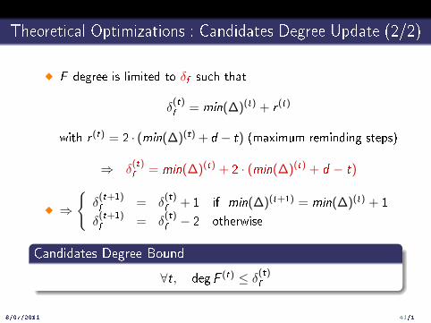
Theoretical Optimizations : Candidates Degree Update (2/2)

� F degree is limited to δf such that

δ(t)f = min(∆)(t) + r (t)

with r (t) = 2 · (min(∆)(t) + d − t) (maximum reminding steps)

⇒ δ(t)f = min(∆)(t) + 2 · (min(∆)(t) + d − t)

� ⇒

{δ(t+1)f = δ

(t)f + 1 if min(∆)(t+1) = min(∆)(t) + 1

δ(t+1)f = δ

(t)f − 2 otherwise

Candidates Degree Bound

∀t, deg F (t) ≤ δ(t)f

grid

thales-logo

8/07/2011 42/1

Outline

grid

thales-logo

8/07/2011 43/1

Outline

grid

thales-logo

8/07/2011 44/1

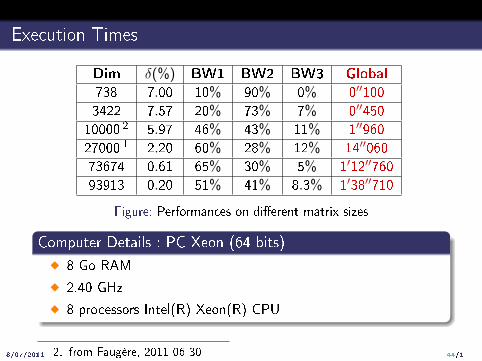
Execution Times

Dim δ(%) BW1 BW2 BW3 Global

738 7.00 10% 90% 0% 0′′100

3422 7.57 20% 73% 7% 0′′450

10000 2 5.97 46% 43% 11% 1′′960

27000 1 2.20 60% 28% 12% 14′′060

73674 0.61 65% 30% 5% 1′12′′760

93913 0.20 51% 41% 8.3% 1′38′′710

Figure: Performances on di�erent matrix sizes

Computer Details : PC Xeon (64 bits)

� 8 Go RAM

� 2.40 GHz

� 8 processors Intel(R) Xeon(R) CPU

2. from Faugère, 2011-06-30

grid

thales-logo

8/07/2011 45/1

Outline

grid

thales-logo

8/07/2011 46/1

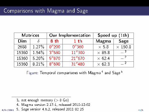
Comparisons with Magma and Sage

Matrices Our Implementation Speed up (1th)

Dim δ 8 th 1 th Magma Sage

2688 1.27% 0′′200 0′′360 × 5.8 × 150.0

15360 1.54% 3′′580 11′′300 × 85.8 − 3

15360 5.20% 5′′870 21′′670 × 62.4 − 2

15360 8.21% 8′′690 31′′480 × 62.3 − 2

Figure: Temporal comparisons with Magma 4 and Sage 5

3. not enough memory (> 8 Go)4. Magma version 2.17-1, released 2010-12-025. Sage version 4.6.2, released 2011-02-25

grid

thales-logo

8/07/2011 47/1

Outline

grid

thales-logo

8/07/2011 48/1

� Summary

• E�cient implementation of the Block Wiedemann algorithmover GF(2) in C language

• Practical and theoretical optimizations

• Encouraging results compared to existing methods

� Further Work

• Algebraic Cryptanalysis of HFE Cryptosystems Using Gröbner

Bases [?] using Block Wiedemann algorithm

• Use of Gröbner bases algorithm [?]

• Comparisons with LinBox

• Work on applications

• Open source ?

grid

thales-logo

8/07/2011 49/1

Bibliography