Solving Large Retrograde Analysis Problems

Using a Network of Workstations

Robert LakeJonathan Schaeffer

Paul Lu

Department of Computing ScienceUniversity of AlbertaEdmonton, AlbertaCanada T6G 2H1

ABSTRACT

Chess endgame databases, while of important theoretical interest, have yet tomake a significant impact in tournament chess. In the game of checkers, how-ever, endgame databases have played a pivotal role in the success of our WorldChampionship challenger program Chinook. Consequently, we are interestedin building databases consisting of hundreds of billions of positions. Sincedatabase positions arise frequently in Chinook’s search trees, the databasesmust be accessible in real-time, unlike in chess. This paper discusses tech-niques for building large endgame databases using a network of workstations,and how this data can be organized for use in a real-time search. Althoughcheckers is used to illustrate many of the ideas, the techniques and toolsdeveloped are also applicable to chess.

1. Introduction

In computer chess, the impact of precomputed endgame databases on tournamentplay has been relatively small. There are primarily three reasons for this. First, thevariety of chess pieces result in different classes of endgames, many of which are rarelyseen in actual play. Second, the outcome of most chess games is usually decided wellbefore the endgame, meaning that even if databases were available, they would rarelyplay a role in determining a game’s outcome. Consequently, few chess programs usenon-trivial databases as part of their real-time search. Third, the substantial computa-tional resources required to build endgame databases in the conventional way [12, 13]makes it difficult for most chess programmers to build their own. Fortunately, however,the databases are being made available to the public [6, 14, 15]. For chess at least, themain benefit of database construction seems to be educational, revealing many newendgame results to the players (see [5] for an interesting example) without, as yet, reveal-ing their secrets ([9] represents one attempt).

Our goal is to build a checkers endgame database of 150 billion positions (all the1-7 piece endgames, and the 4×4 subset of the 8-piece endgames). This paper discussestechniques for building large endgame databases using a network of workstations, andhow this data can be organized for use in a real-time search.

- 2 -

This work has been applied to the domain of computer checkers (8 × 8 draughts),which is an interesting point of comparison for computer chess. In checkers, since thereare only checker and king pieces, all games play into a limited set of endgame classes.Also, the lower branching factor of checkers trees and the forced captures of the gameresult in deeper search trees than in chess. Although the root of the tree may be far fromthe endgame, the leaf nodes already may be in the databases. Consequently, the utility ofthe endgame databases is higher in checkers than chess.

Computing the checkers endgame databases with the resources available to us hasbeen a challenge. The problem requires excessive memory, time, I/O and mass storage tosolve using either the sequential version of Thompson’s algorithm [4, 13] or Stiller’svector-processing method [12]. Of course, as computers get more powerful, many ofthese problems will be overcome, but we want the databases now! Other approaches tosolving the problem, such as proving some properties of the search space (an interestingexample can be found in [2]), have not been successful.

The memory problem is addressed by decomposing the 150 billion positions wewant to solve into small pieces (10 million positions) and solving them individually. Thetime problem is solved using a distributed network of heterogeneous workstations. TheI/O problem is (partially) solved by dividing the computation into distinct phases orpasses to eliminate redundant I/O. The mass storage problem is solved by anapplication-dependent compression algorithm that also allows real-time access. Interest-ingly, the problem has been sufficiently decomposed that a single modern workstationcan be used to solve the entire problem. The same techniques can be applied to buildingchess endgames databases.

More generally, the construction of endgame databases may have a greater impactthan just in computer game playing. Many problems in mathematics and the sciencesrequire finding the optimal solution in a large combinatorial search space. In essence, theconstruction of an endgame database is a backwards search from the solution. Whencombined with a forward search tree, as with computer games, the optimal solution maybe found in less time. Therefore, some types of optimization problems can benefit fromthe approach taken in this paper.

The success of the Chinook checkers program (8 × 8 draughts) is largely due to itsendgame databases [10]. The project began in June 1989 with the short-term goal ofdeveloping a program capable of defeating the human world champion and the long-termgoal of solving the game. Chinook has achieved significant successes and also has hadsome setbacks. It was the first program to earn the right to play a reigning world cham-pion for the title by placing second to then World Champion, Dr. Marion Tinsley, at theU.S. National Open in 1990, the biennial event for the determining the next challenger.At the 1992 Silicon Graphics World Draughts Championship in London, Dr. Tinsleydefeated Chinook with 4 wins, 2 losses and 33 draws [11]. Previous to that match, Dr.Tinsley had lost only 7 games in over 40 years of competitive play. The techniquesdescribed in this paper have allowed us to significantly increase the number of positionsin the endgame databases available to Chinook for the next Tinsley-Chinook match, ten-tatively scheduled for 1994.

- 3 -

2. Retrograde Analysis

Retrograde analysis can be used to help solve a large combinatorial search space bybuilding the optimal solution in a bottom-up manner (searching from the solution back-wards towards the problem statement). With an appropriate top-down search algorithm(searching from the problem statement forwards towards a solution), a better approximatesolution, or possibly the optimal solution, can be obtained. For our problem domain,solving the game of checkers, the search space consists of 5 × 1020 positions.

The construction of a checkers endgame database is simply the computation of atransitive closure. Each position is a member of either the set of wins, losses or draws.Once computed, the classification of a database entry represents perfect knowledge as tothe theoretical value of that position. Since a checkers database is a lookup table test forset membership, the simple techniques discussed in this paper can be applied to otherproblem domains.

Initially, all positions are given the value of unknown. Some of the positions canbe classified as either a win or a loss according the the rules of the game. For exam-ple, a player without any pieces on the board (i.e. without material) or without a legalmove is a loss in checkers. The set membership of the other positions depends on themembership of positions reachable by the legal moves of the game. Given a sufficientamount of information, the classification of a position can be changed from unknown toeither a win, loss or draw. Specifically, if the side to play has a legal move that leads to aposition that has already been classified as a win for itself, then the current position isalso a win. If the side to play only has legal moves leading to positions that are wins forthe opponent, then its current position is a loss for itself. The transitive closure is com-plete when there is insufficient information to change the value of any other positions.At that point, all of the unknown positions are declared to be draws since neither playercan force a win.

In theory, if all of the leaf nodes of the minimax game tree are from the endgamedatabases, then there is no error in the evaluation of the root position. Consequently, itmay be possible to compute the game theoretic value of the game of checkers using theperfect knowledge of the endgame databases. In practice, such as playing a game underreal-time constraints, limitations on time and space may not allow the search to extend allof the leaf nodes into the endgame databases. For each leaf node not in the databases, aheuristic evaluation function is used to assess the position. Each application of theevaluation function introduces the possibility of error. A combination of leaf nodes fromthe databases and from the evaluation function is the most common situation. As the per-cent of leaf nodes taken from the databases increases, the accuracy of the search resultimproves.

The goal of our project is to solve 150 billion checkers positions. A naive approachto tackling the problem would exceed the computational, storage and input-output (I/O)facilities of most current day computers. Of course, computers continue to increase intheir capabilities, but solving the problem with the current technology requires a morerefined approach. Furthermore, although there may exist computers capable of dealingwith the size of the endgame database problem, they are neither affordable or available tothis team of researchers. The design tradeoffs and issues relating to solving large prob-lems with limited resources is both challenging and important. There will always be

- 4 -

problems that are technologically feasible, but too large to solve with the resources avail-able. In fact, a simple implementation of retrograde analysis would be CPU-bound,memory-bound and I/O-bound, the classic triad of a large computational problem. In thefollowing sections, each of these bottlenecks is addressed.

3. Basic Algorithm

All endgame databases are built according to the number of pieces on the board.Constructing an N-piece endgame database requires enumerating all positions with Npieces and computing whether each position is a win, loss, or draw. All database entriesdescribe positions with Black to move. White to move results are determined by revers-ing the board, changing the colors of the pieces, and retrieving the appropriate Black tomove result.

An N-piece database is computed using an iterative algorithm, building on theresults of the previously computed 1, 2, ..., (N-1)-piece databases, as per a backwardssearch. Initially all N-piece positions are viewed as having a value of UNKNOWN. Eachiteration scans through a subset of the positions to determine whether there is enoughinformation to change a position’s value to WIN, LOSS or DRAW. This is idea behindThompson’s original algorithm [13].

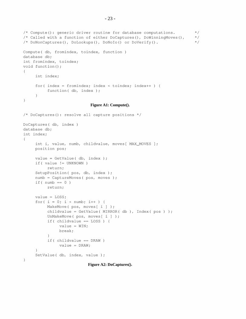
The execution strategy of the first iterative pass depends on an important rule ofcheckers: a capture must be played when one or more capture moves are present amongthe available legal moves. As a result, the first pass determines the value of all capturepositions and defers the rest for later passes (analogous to resolving all mate positions inchess). Since a capture leads to a position with N-1 or fewer pieces, each N-piece cap-ture position is resolved by retrieving the values from the previously computed databasesfor N-1 or fewer pieces. The capture position is then assigned the highest valueretrieved from the previously computed positions. These values are ranked in descendingorder as win, draw and loss (hence 2 bits of storage per position †). Approximately halfof the positions in a database are capture positions. In Appendix A, the pseudo-code forthe DoCaptures() routine is given.

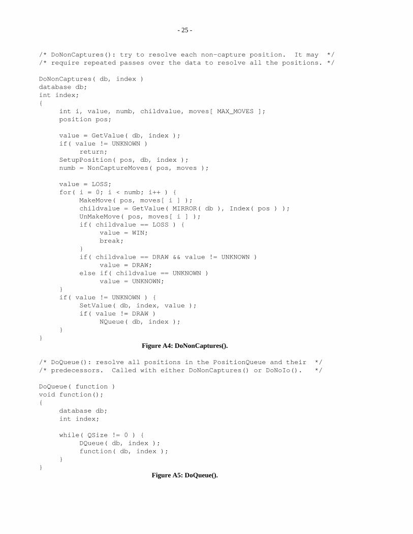
The second and subsequent iterations through the database resolve only non-capturepositions. For each position considered, all the legal moves are generated. Each move isexecuted and the resulting position’s value is retrieved from the current N-piece data-base. The unknown position is assigned a value only when one of the legal moves resultsin a win or all legal moves have been resolved. The program iterates until no more N-piece positions can be resolved (DoNonCaptures() in Appendix A). At that point, allremaining unknown positions are set to draws.

This algorithm is summarized in Figure 1. This method resolves positions in orderof least to most moves required to play into a lesser database. Thus, the algorithm can beapplied to problems such as finding all wins in 1 move, then 2, then 3, and so on.

There are, in fact, two opposite approaches to resolving unknown positions. The"forward" approach described above takes each unresolved position, generates its succes-sor positions, and from these tries to determine the value of the parent. The "backward"approach takes a resolved position, uses a reverse move generator to find its predecessor_ ______________Some implementations use 1 bit per position. The justification for 2 bits is given in Section 3.3.

- 5 -

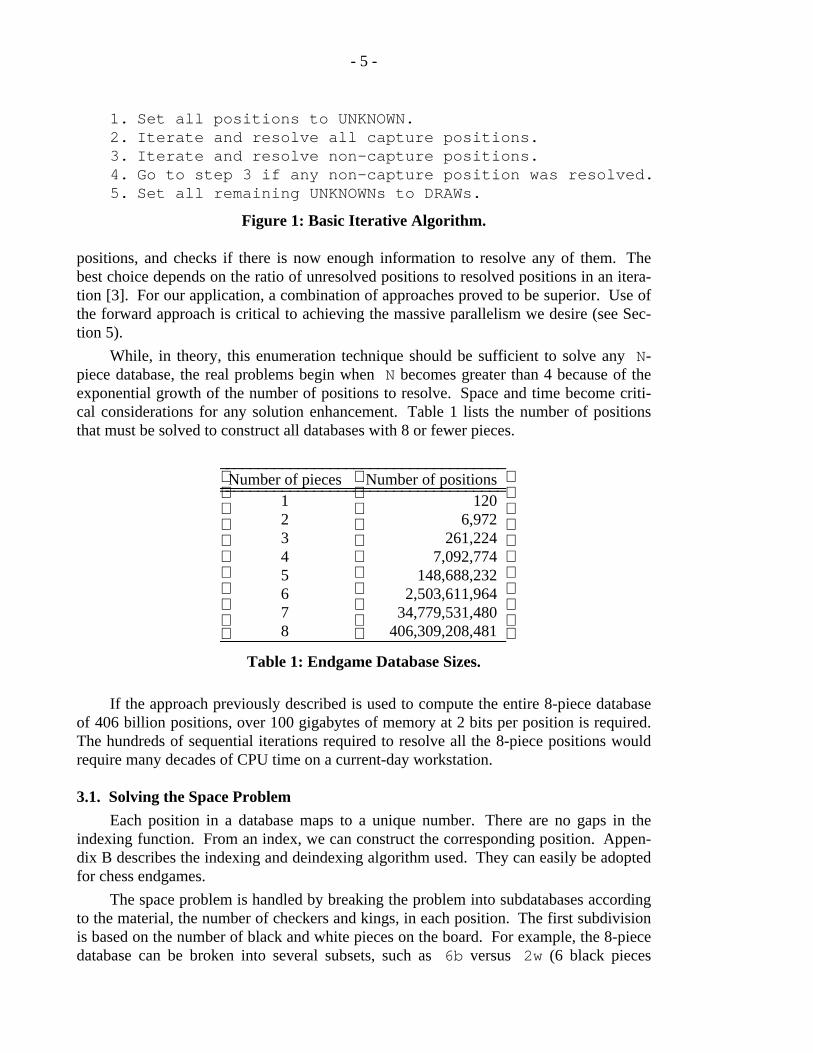
1. Set all positions to UNKNOWN.2. Iterate and resolve all capture positions.3. Iterate and resolve non-capture positions.4. Go to step 3 if any non-capture position was resolved.5. Set all remaining UNKNOWNs to DRAWs.

Figure 1: Basic Iterative Algorithm.

positions, and checks if there is now enough information to resolve any of them. Thebest choice depends on the ratio of unresolved positions to resolved positions in an itera-tion [3]. For our application, a combination of approaches proved to be superior. Use ofthe forward approach is critical to achieving the massive parallelism we desire (see Sec-tion 5).

While, in theory, this enumeration technique should be sufficient to solve any N-piece database, the real problems begin when N becomes greater than 4 because of theexponential growth of the number of positions to resolve. Space and time become criti-cal considerations for any solution enhancement. Table 1 lists the number of positionsthat must be solved to construct all databases with 8 or fewer pieces.

_ ___________________________________Number of pieces Number of positions_ ____________________________________ ___________________________________

1 1202 6,9723 261,2244 7,092,7745 148,688,2326 2,503,611,9647 34,779,531,4808 406,309,208,481_ ___________________________________

Table 1: Endgame Database Sizes.

If the approach previously described is used to compute the entire 8-piece databaseof 406 billion positions, over 100 gigabytes of memory at 2 bits per position is required.The hundreds of sequential iterations required to resolve all the 8-piece positions wouldrequire many decades of CPU time on a current-day workstation.

3.1. Solving the Space Problem

Each position in a database maps to a unique number. There are no gaps in theindexing function. From an index, we can construct the corresponding position. Appen-dix B describes the indexing and deindexing algorithm used. They can easily be adoptedfor chess endgames.

The space problem is handled by breaking the problem into subdatabases accordingto the material, the number of checkers and kings, in each position. The first subdivisionis based on the number of black and white pieces on the board. For example, the 8-piecedatabase can be broken into several subsets, such as 6b versus 2w (6 black pieces

- 6 -

against 2 white) or 4b versus 4w. Table 2 shows the number of database positionswithin each subset. The entries where one side has 0 pieces, a loss by the rules of thegame, are not included.

_ ________________________________________________________________________________________________________

Black White Pieces

Pieces _________________________________________________________________________________________________

1 2 3 4 5 6 7_ _________________________________________________________________________________________________________ ________________________________________________________________________________________________________1 23,488 98,016 1,773,192 23,204,660 233,999,928 1,891,451,952 12,586,073,760

2 98,016 2,662,932 46,520,744 587,139,846 5,702,475,480 44,328,555,960

3 1,773,192 46,520,744 783,806,128 9,527,629,380 88,991,228,360

4 23,204,660 587,139,846 9,527,629,380 111,378,534,401

5 233,999,928 5,702,475,480 88,991,228,360

6 1,891,451,952 44,328,555,960

7 12,586,073,760_ ________________________________________________________________________________________________________

Table 2: Subdividing the Database.

The second subdivision is based on the number of kings and checkers. Since check-ers can promote into kings, but not visa-versa, positions in a database with k kings cannever play into positions with the same number of pieces and less than k kings. Hence,these subsets can be further broken down by computing king-only positions first andworking backwards towards checker-only positions.

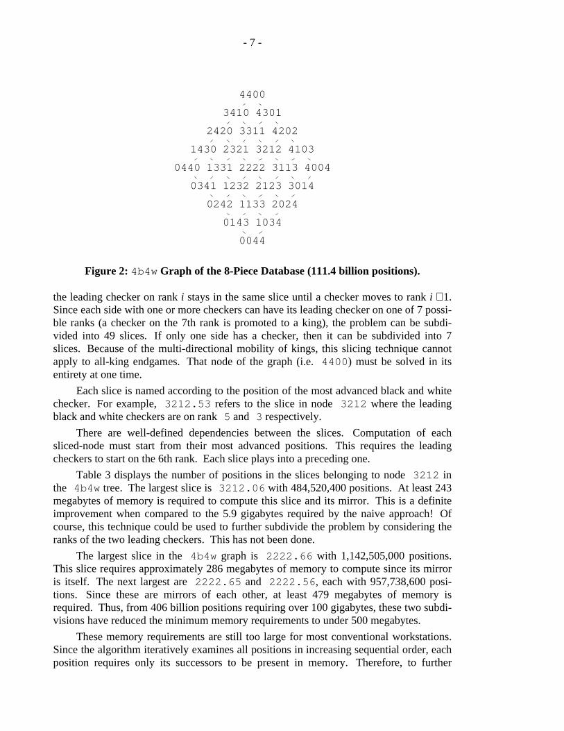
This subdivision can be represented by a set of graphs. Each graph contains allpositions composed of b black pieces and w white pieces. The nodes represent subdata-bases holding positions with similar numbers of kings and checkers. Figure 2 shows thesubdivision of the 4b versus 4w positions. Each node is named using four digits torepresent the number of black kings, white kings, black checkers, and white checkers inthe subdatabase. The first subdatabase computed is 4400 (4 kings versus 4 kings) andthe last is 0044 (4 checkers versus 4 checkers).

Because lower node positions lead to upper node positions, all database computa-tions begin at the top of each graph and fan downward. Since every position must beresolved for both color’s turn to play, each database computation requires two nodes: theactive (or original) database and its mirror. The mirror is defined as the node (or graph)where the colors are reversed. For example, the mirror for node 4112 in the 5b3wgraph is node 1421 in the 3b5w graph. While most nodes have mirrors in a separategraph, a few nodes have their mirror in the same graph.

Although this database partitioning into graphs helps reduce space difficulties,many of the nodes are still too large to calculate on most computers. For example, node3212 in the 4b4w graph contains 11,799,496,800 positions. When combined with itsmirror, the memory requirement to compute the entire subdatabase is at least 5.9 giga-bytes.

The key to solving nodes this large is to partition the subdatabase into yet smallerparts. The approach used is to slice the positions up based on the rank of the leading(most advanced) checker for each side. The ranks are numbered 0 to 7. A position with

- 7 -

4400

3410 4301

2420 3311 4202

1430 2321 3212 4103

0440 1331 2222 3113 4004

0341 1232 2123 3014

0242 1133 2024

0143 1034

0044

Figure 2: 4b4w Graph of the 8-Piece Database (111.4 billion positions).

the leading checker on rank i stays in the same slice until a checker moves to rank i + 1.Since each side with one or more checkers can have its leading checker on one of 7 possi-ble ranks (a checker on the 7th rank is promoted to a king), the problem can be subdi-vided into 49 slices. If only one side has a checker, then it can be subdivided into 7slices. Because of the multi-directional mobility of kings, this slicing technique cannotapply to all-king endgames. That node of the graph (i.e. 4400) must be solved in itsentirety at one time.

Each slice is named according to the position of the most advanced black and whitechecker. For example, 3212.53 refers to the slice in node 3212 where the leadingblack and white checkers are on rank 5 and 3 respectively.

There are well-defined dependencies between the slices. Computation of eachsliced-node must start from their most advanced positions. This requires the leadingcheckers to start on the 6th rank. Each slice plays into a preceding one.

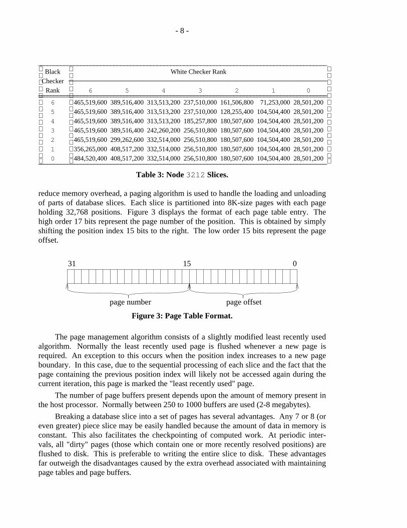
Table 3 displays the number of positions in the slices belonging to node 3212 inthe 4b4w tree. The largest slice is 3212.06 with 484,520,400 positions. At least 243megabytes of memory is required to compute this slice and its mirror. This is a definiteimprovement when compared to the 5.9 gigabytes required by the naive approach! Ofcourse, this technique could be used to further subdivide the problem by considering theranks of the two leading checkers. This has not been done.

The largest slice in the 4b4w graph is 2222.66 with 1,142,505,000 positions.This slice requires approximately 286 megabytes of memory to compute since its mirroris itself. The next largest are 2222.65 and 2222.56, each with 957,738,600 posi-tions. Since these are mirrors of each other, at least 479 megabytes of memory isrequired. Thus, from 406 billion positions requiring over 100 gigabytes, these two subdi-visions have reduced the minimum memory requirements to under 500 megabytes.

These memory requirements are still too large for most conventional workstations.Since the algorithm iteratively examines all positions in increasing sequential order, eachposition requires only its successors to be present in memory. Therefore, to further

- 8 -

_ ______________________________________________________________________________________Black White Checker Rank

Checker _ _____________________________________________________________________________

Rank 6 5 4 3 2 1 0_ _______________________________________________________________________________________ ______________________________________________________________________________________6 465,519,600 389,516,400 313,513,200 237,510,000 161,506,800 71,253,000 28,501,200

5 465,519,600 389,516,400 313,513,200 237,510,000 128,255,400 104,504,400 28,501,200

4 465,519,600 389,516,400 313,513,200 185,257,800 180,507,600 104,504,400 28,501,200

3 465,519,600 389,516,400 242,260,200 256,510,800 180,507,600 104,504,400 28,501,200

2 465,519,600 299,262,600 332,514,000 256,510,800 180,507,600 104,504,400 28,501,200

1 356,265,000 408,517,200 332,514,000 256,510,800 180,507,600 104,504,400 28,501,200

0 484,520,400 408,517,200 332,514,000 256,510,800 180,507,600 104,504,400 28,501,200_ ______________________________________________________________________________________

Table 3: Node 3212 Slices.

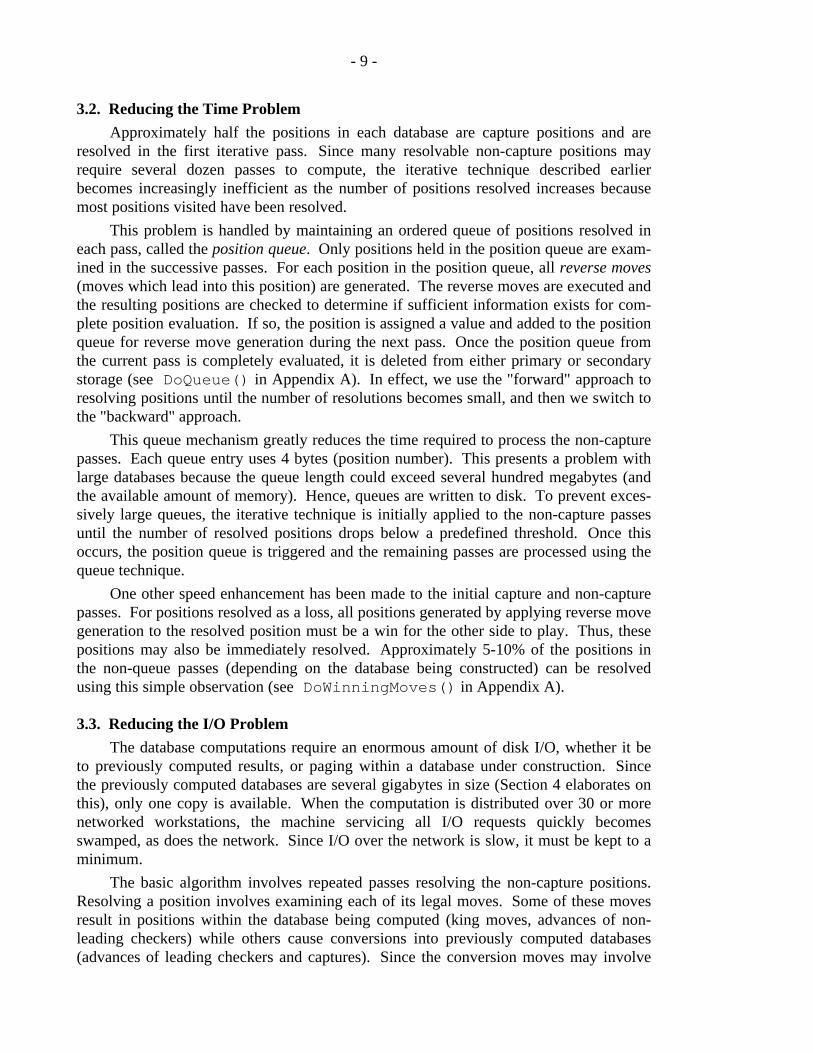
reduce memory overhead, a paging algorithm is used to handle the loading and unloadingof parts of database slices. Each slice is partitioned into 8K-size pages with each pageholding 32,768 positions. Figure 3 displays the format of each page table entry. Thehigh order 17 bits represent the page number of the position. This is obtained by simplyshifting the position index 15 bits to the right. The low order 15 bits represent the pageoffset.

0 15 31

page number page offset

Figure 3: Page Table Format.

The page management algorithm consists of a slightly modified least recently usedalgorithm. Normally the least recently used page is flushed whenever a new page isrequired. An exception to this occurs when the position index increases to a new pageboundary. In this case, due to the sequential processing of each slice and the fact that thepage containing the previous position index will likely not be accessed again during thecurrent iteration, this page is marked the "least recently used" page.

The number of page buffers present depends upon the amount of memory present inthe host processor. Normally between 250 to 1000 buffers are used (2-8 megabytes).

Breaking a database slice into a set of pages has several advantages. Any 7 or 8 (oreven greater) piece slice may be easily handled because the amount of data in memory isconstant. This also facilitates the checkpointing of computed work. At periodic inter-vals, all "dirty" pages (those which contain one or more recently resolved positions) areflushed to disk. This is preferable to writing the entire slice to disk. These advantagesfar outweigh the disadvantages caused by the extra overhead associated with maintainingpage tables and page buffers.

- 9 -

3.2. Reducing the Time Problem

Approximately half the positions in each database are capture positions and areresolved in the first iterative pass. Since many resolvable non-capture positions mayrequire several dozen passes to compute, the iterative technique described earlierbecomes increasingly inefficient as the number of positions resolved increases becausemost positions visited have been resolved.

This problem is handled by maintaining an ordered queue of positions resolved ineach pass, called the position queue. Only positions held in the position queue are exam-ined in the successive passes. For each position in the position queue, all reverse moves(moves which lead into this position) are generated. The reverse moves are executed andthe resulting positions are checked to determine if sufficient information exists for com-plete position evaluation. If so, the position is assigned a value and added to the positionqueue for reverse move generation during the next pass. Once the position queue fromthe current pass is completely evaluated, it is deleted from either primary or secondarystorage (see DoQueue() in Appendix A). In effect, we use the "forward" approach toresolving positions until the number of resolutions becomes small, and then we switch tothe "backward" approach.

This queue mechanism greatly reduces the time required to process the non-capturepasses. Each queue entry uses 4 bytes (position number). This presents a problem withlarge databases because the queue length could exceed several hundred megabytes (andthe available amount of memory). Hence, queues are written to disk. To prevent exces-sively large queues, the iterative technique is initially applied to the non-capture passesuntil the number of resolved positions drops below a predefined threshold. Once thisoccurs, the position queue is triggered and the remaining passes are processed using thequeue technique.

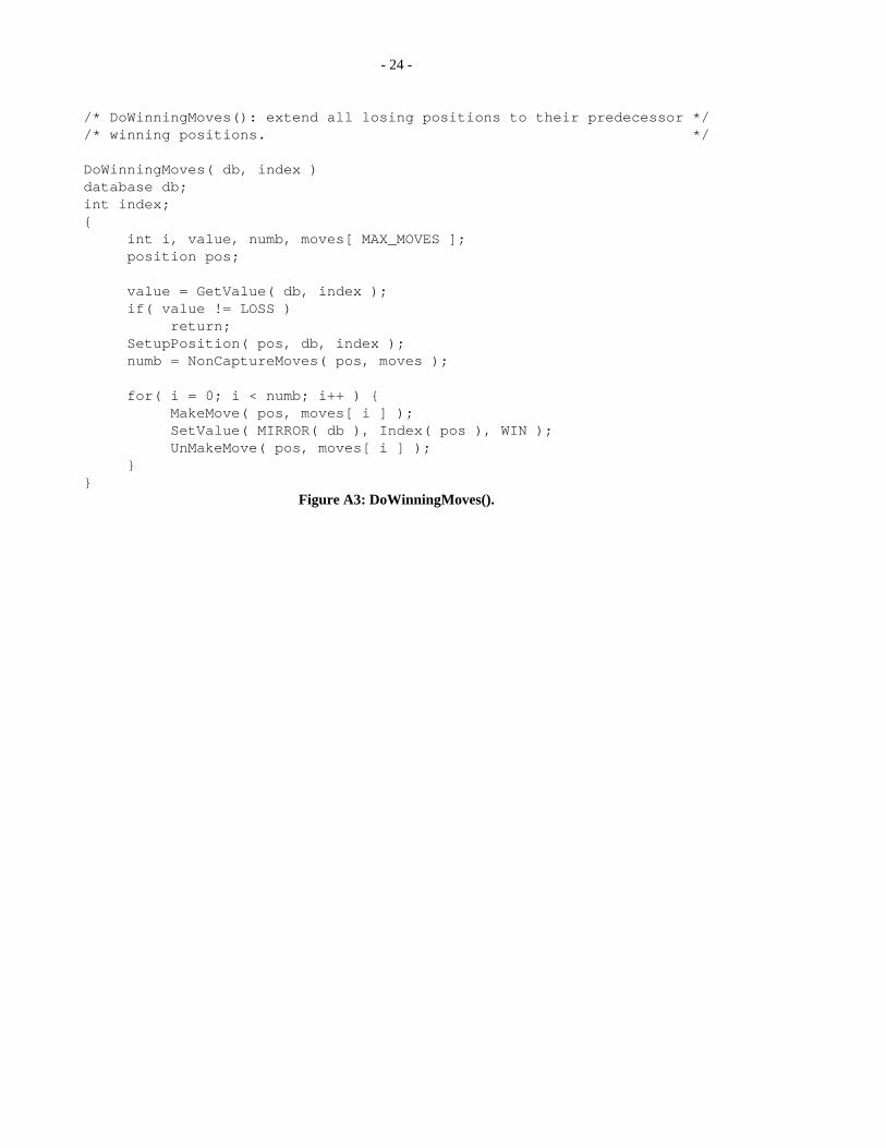
One other speed enhancement has been made to the initial capture and non-capturepasses. For positions resolved as a loss, all positions generated by applying reverse movegeneration to the resolved position must be a win for the other side to play. Thus, thesepositions may also be immediately resolved. Approximately 5-10% of the positions inthe non-queue passes (depending on the database being constructed) can be resolvedusing this simple observation (see DoWinningMoves() in Appendix A).

3.3. Reducing the I/O Problem

The database computations require an enormous amount of disk I/O, whether it beto previously computed results, or paging within a database under construction. Sincethe previously computed databases are several gigabytes in size (Section 4 elaborates onthis), only one copy is available. When the computation is distributed over 30 or morenetworked workstations, the machine servicing all I/O requests quickly becomesswamped, as does the network. Since I/O over the network is slow, it must be kept to aminimum.

The basic algorithm involves repeated passes resolving the non-capture positions.Resolving a position involves examining each of its legal moves. Some of these movesresult in positions within the database being computed (king moves, advances of non-leading checkers) while others cause conversions into previously computed databases(advances of leading checkers and captures). Since the conversion moves may involve

- 10 -

I/O, and they are repeated every time a position is revisited, it is desirable to obtain thisinformation once, thereby reducing the I/O.

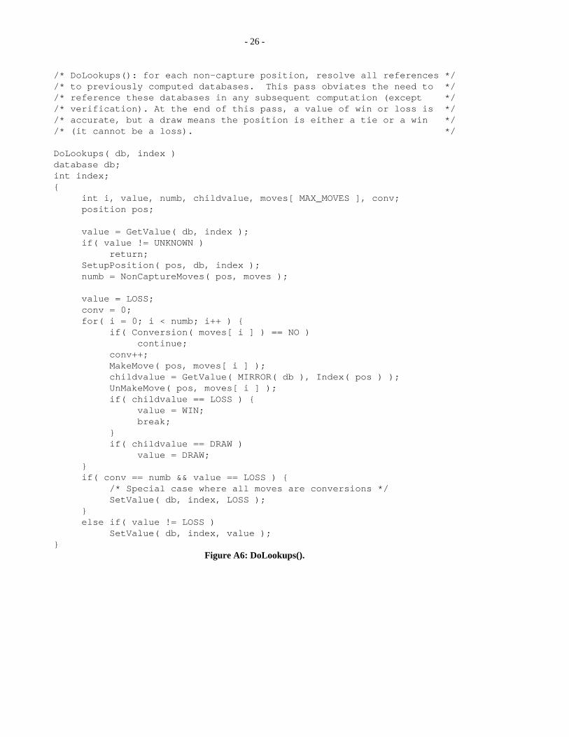
The non-capture pass has been broken up into two components. The first, calledDoLookups(), takes each non-capture position and looks up each legal conversionmove and stores the results of this I/O back in the database. The second, DoNoIo(),then uses the I/O information to do repeated passes through the data, only doing I/O onthe current database and never having to refer back to a previously computed result.Appendix A contains pseudo-code for both DoLookups() and DoNoIo().

Each position can take on one of 4 values. DoLookups() takes advantage of the2-bit per position representation to encode the result of the conversion moves. Themeaning of a position value of WIN or LOSS remains unchanged. The value of DRAWmeans that the conversion moves imply that this position has a value of DRAW or better.In other words, there is at least one conversion move leading to a draw, but none to a win.Thus, consideration of the non-conversion moves can only leave the value as a DRAW orpossibly improve it to a WIN. A value of UNKNOWN implies that consideration of theconversion moves gave no lower bound on the value of the position (i.e. any of WIN,LOSS or DRAW is still possible). The result of DoLookups() is either an accurateresult or a lower bound value for each non-capture position.

DoNoIo() essentially iterates through all DRAW and UNKNOWN values trying toimprove the value. Any resolved position is added to the queue for further processing.The value of a position is never allowed to go below that set by DoLookups().

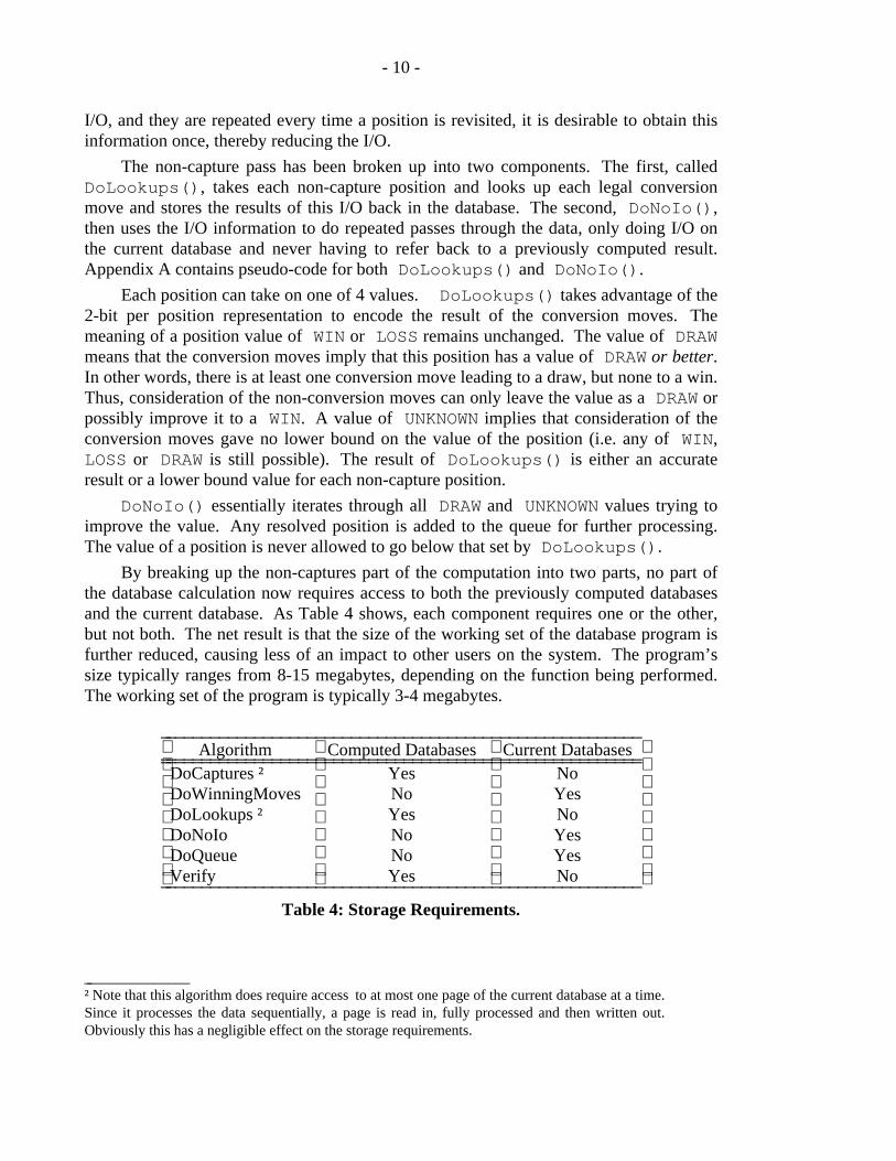
By breaking up the non-captures part of the computation into two parts, no part ofthe database calculation now requires access to both the previously computed databasesand the current database. As Table 4 shows, each component requires one or the other,but not both. The net result is that the size of the working set of the database program isfurther reduced, causing less of an impact to other users on the system. The program’ssize typically ranges from 8-15 megabytes, depending on the function being performed.The working set of the program is typically 3-4 megabytes.

_ ______________________________________________________Algorithm Computed Databases Current Databases_ _______________________________________________________ ______________________________________________________

DoCaptures † Yes NoDoWinningMoves No YesDoLookups † Yes NoDoNoIo No YesDoQueue No YesVerify Yes No_ ______________________________________________________

Table 4: Storage Requirements.

_ ______________† Note that this algorithm does require access to at most one page of the current database at a time.Since it processes the data sequentially, a page is read in, fully processed and then written out.Obviously this has a negligible effect on the storage requirements.

- 11 -

3.4. Putting it all Together

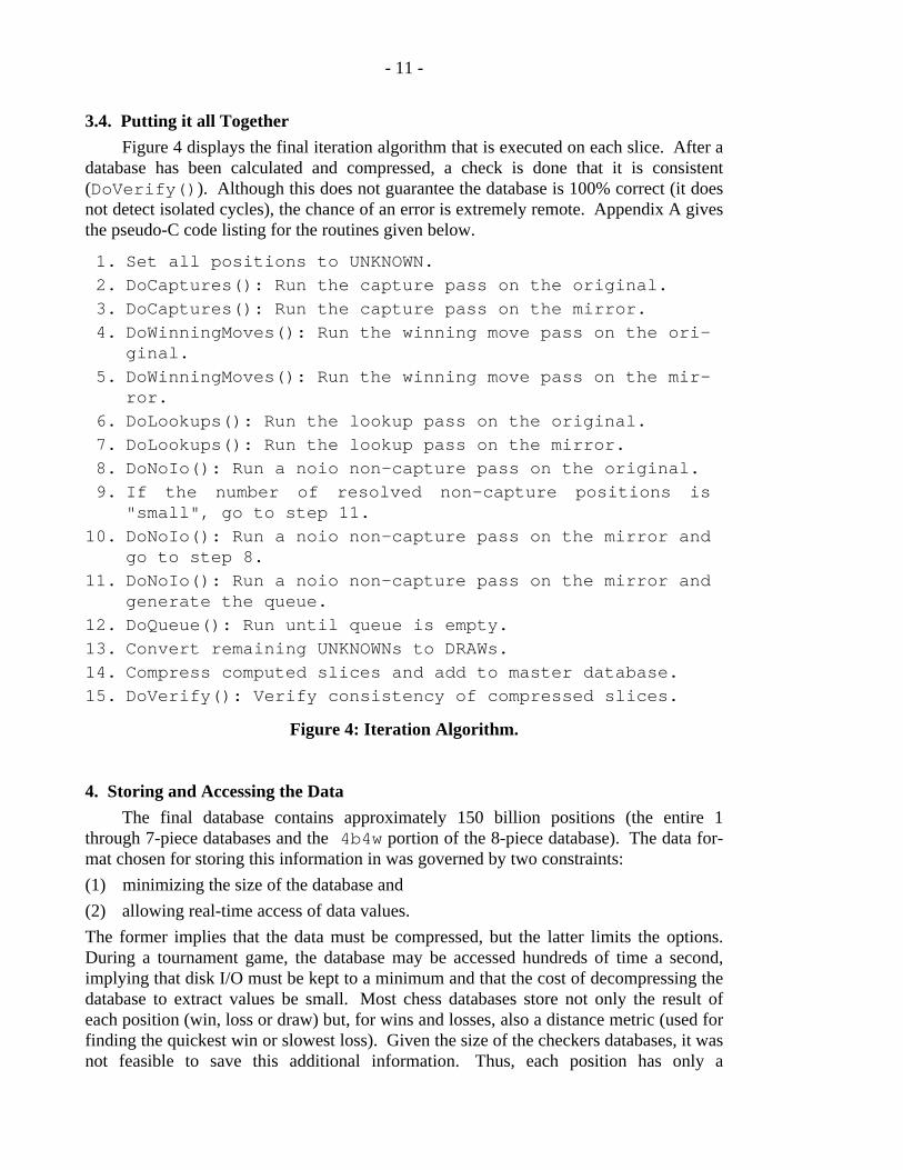
Figure 4 displays the final iteration algorithm that is executed on each slice. After adatabase has been calculated and compressed, a check is done that it is consistent(DoVerify()). Although this does not guarantee the database is 100% correct (it doesnot detect isolated cycles), the chance of an error is extremely remote. Appendix A givesthe pseudo-C code listing for the routines given below.

Set all positions to UNKNOWN. 1.

DoCaptures(): Run the capture pass on the original. 2.

DoCaptures(): Run the capture pass on the mirror. 3.

DoWinningMoves(): Run the winning move pass on the ori-ginal.

4.

DoWinningMoves(): Run the winning move pass on the mir-ror.

5.

DoLookups(): Run the lookup pass on the original. 6.

DoLookups(): Run the lookup pass on the mirror. 7.

DoNoIo(): Run a noio non-capture pass on the original. 8.

If the number of resolved non-capture positions is"small", go to step 11.

9.

DoNoIo(): Run a noio non-capture pass on the mirror andgo to step 8.

10.

DoNoIo(): Run a noio non-capture pass on the mirror andgenerate the queue.

11.

DoQueue(): Run until queue is empty. 12.

Convert remaining UNKNOWNs to DRAWs. 13.

Compress computed slices and add to master database. 14.

DoVerify(): Verify consistency of compressed slices. 15.

Figure 4: Iteration Algorithm.

4. Storing and Accessing the Data

The final database contains approximately 150 billion positions (the entire 1through 7-piece databases and the 4b4w portion of the 8-piece database). The data for-mat chosen for storing this information in was governed by two constraints:

(1) minimizing the size of the database and

(2) allowing real-time access of data values.

The former implies that the data must be compressed, but the latter limits the options.During a tournament game, the database may be accessed hundreds of time a second,implying that disk I/O must be kept to a minimum and that the cost of decompressing thedatabase to extract values be small. Most chess databases store not only the result ofeach position (win, loss or draw) but, for wins and losses, also a distance metric (used forfinding the quickest win or slowest loss). Given the size of the checkers databases, it wasnot feasible to save this additional information. Thus, each position has only a

- 12 -

win/loss/draw designation. Note that under this scenario, it is possible for Chinook toreach a database win but be unable to win it because it cannot search far enough ahead tofind a conversion into another subdatabase. This has never happened.

Five position values can be stored in a byte (35 = 243 < 256). This naive compres-sion results in 150 billion positions requiring 30 gigabytes of disk storage. Unfor-tunately, with today’s technology, this is an expensive proposition. Numerous schemeshave been tried to gain further compression. Some achieve high compression ratios, butat a prohibitive run-time decompression cost. Others, such as the 5 positions per bytescheme, have minimal decompression costs but low compression ratios. In this report,only the scheme finally chosen will be discussed in detail (the scheme described in [10]is not quite as efficient). One failed attempt worth mentioning was the use of an evalua-tion function to predict the value of a position (a technique used for compressing chessgames [1]). If the routine was sufficiently accurate, then only exception positions needbe stored. While seemingly a promising approach, we were never able to develop a func-tion that gave better results than the scheme eventually chosen. Finally, because of thepresence of checkers and the non-symmetric nature of the board, one cannot take advan-tage of symmetries, as is possible in chess.

In the game of checkers, capture moves are forced. They have the same affect onthe game tree as do checking moves in chess; the branching factor drops to an average of1.3 [8]. Since capture positions comprise roughly half of all positions in the database,these positions can be omitted since their result can be easily computed. In a search, if acapture position in a database is reached, it is searched an additional ply deeper to find itsvalue. Further, positions where one side could capture if the side-to-move were switchedcomprise an additional 25% of the positions (capture-threat). Again, by removing thesepositions from the database, additional compression can be achieved, at the cost of amore complicated search algorithm for resolving values.

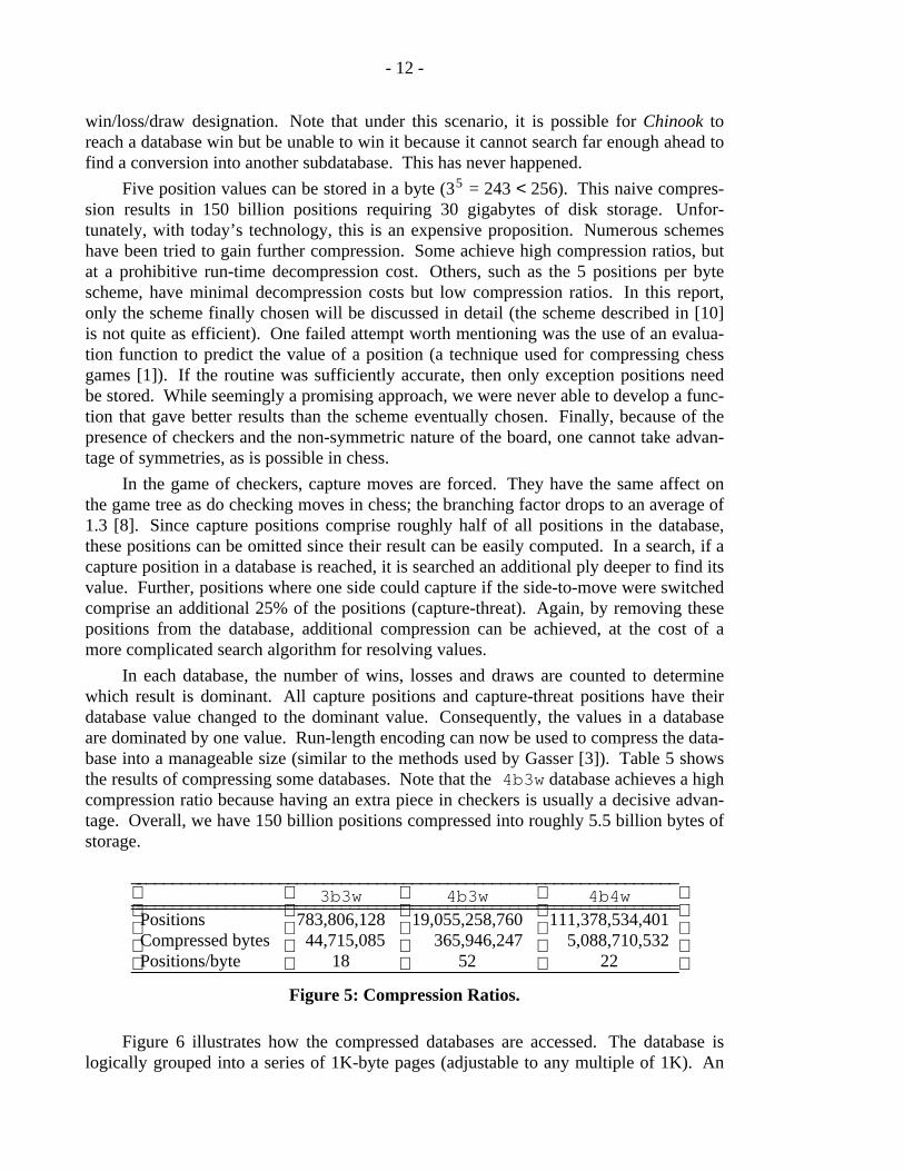
In each database, the number of wins, losses and draws are counted to determinewhich result is dominant. All capture positions and capture-threat positions have theirdatabase value changed to the dominant value. Consequently, the values in a databaseare dominated by one value. Run-length encoding can now be used to compress the data-base into a manageable size (similar to the methods used by Gasser [3]). Table 5 showsthe results of compressing some databases. Note that the 4b3w database achieves a highcompression ratio because having an extra piece in checkers is usually a decisive advan-tage. Overall, we have 150 billion positions compressed into roughly 5.5 billion bytes ofstorage.

_ _____________________________________________________________3b3w 4b3w 4b4w_ ______________________________________________________________ _____________________________________________________________

Positions 783,806,128 19,055,258,760 111,378,534,401Compressed bytes 44,715,085 365,946,247 5,088,710,532Positions/byte 18 52 22_ _____________________________________________________________

Figure 5: Compression Ratios.

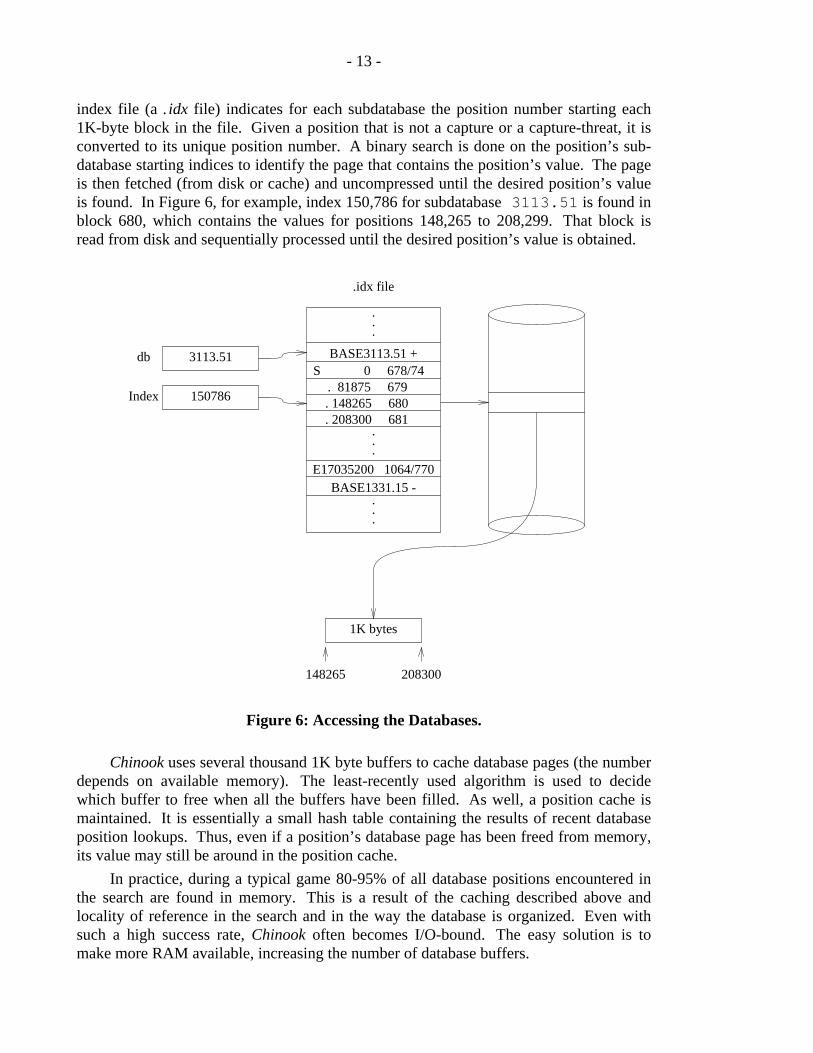
Figure 6 illustrates how the compressed databases are accessed. The database islogically grouped into a series of 1K-byte pages (adjustable to any multiple of 1K). An

- 13 -

index file (a . idx file) indicates for each subdatabase the position number starting each1K-byte block in the file. Given a position that is not a capture or a capture-threat, it isconverted to its unique position number. A binary search is done on the position’s sub-database starting indices to identify the page that contains the position’s value. The pageis then fetched (from disk or cache) and uncompressed until the desired position’s valueis found. In Figure 6, for example, index 150,786 for subdatabase 3113.51 is found inblock 680, which contains the values for positions 148,265 to 208,299. That block isread from disk and sequentially processed until the desired position’s value is obtained.

3113.51 db

150786 Index

.idx file

BASE3113.51 +S 0 678/74

. 81875 679. 148265 680. 208300 681

E17035200 1064/770BASE1331.15 -

.

.

.

.

.

.

.

.

.

1K bytes

148265 208300

Figure 6: Accessing the Databases.

Chinook uses several thousand 1K byte buffers to cache database pages (the numberdepends on available memory). The least-recently used algorithm is used to decidewhich buffer to free when all the buffers have been filled. As well, a position cache ismaintained. It is essentially a small hash table containing the results of recent databaseposition lookups. Thus, even if a position’s database page has been freed from memory,its value may still be around in the position cache.

In practice, during a typical game 80-95% of all database positions encountered inthe search are found in memory. This is a result of the caching described above andlocality of reference in the search and in the way the database is organized. Even withsuch a high success rate, Chinook often becomes I/O-bound. The easy solution is tomake more RAM available, increasing the number of database buffers.

- 14 -

5. Parallelism

While an entire database may be computed sequentially on a single workstationusing the algorithm presented in Figure 4, in reality many workstations work simultane-ously on many databases by taking advantage of three types of parallelism provided bythe database structure and two from the iteration algorithm design.

The first database parallelism opportunity occurs with the database subsets sortedaccording to the number of black and white pieces. These form independent subsetsbecause no position from one subset with N pieces play into positions from another Npiece subset. This enables subsets such as 4b4w and 5b3w to be computed indepen-dently.

The second database parallelism occurs within the graphs describing each subset(for example, Figure 2). All nodes horizontally adjacent to each other may be computedin parallel because positions within one node never lead to positions in same level nodes.The only exception occurs with symmetric graphs because some horizontal nodes may bemirrors of each other. For example, referring to Figure 2 again, nodes 2222,3113/1331 and 4004/0440 may be computed in parallel.

The third database parallelism occurs with the ranks of the leading checker. Eachgraph node is computed diagonally downward from the highest to lowest rank. Figure 7displays the order of computation for a 49-slice node. All entries along each diagonal arecomputed in parallel provided any two diagonal squares are not mirrors of each other.

6 5 4 3 2 1 0

6

5

4

3

2

1

0

White Rank

BlackRank

Figure 7: Leading Checker Rank Parallelism.

Many steps in the iteration algorithm are frequently computed in parallel for severaldatabase slices simultaneously. For example, the DoCaptures pass may be computedin parallel on any number of N-piece slices since this pass references only previouslycomputed databases with N-1 or fewer pieces. Another example is the DoLookupsand DoVerify phase; they can execute on the original and mirror simultaneously.

Despite using the parallelism described above, many difficulties and inefficienciesstill exist with the computations. If each slice is given to a single workstation for execu-tion, computation time is wasted because of differing slice sizes and machine speeds.Occasionally a workstation may handle a very large slice (such as 2222.66) whichrequires several days to compute. This creates a bottleneck for processors waiting to

- 15 -

compute the next set of slices. Since most slices differ in size, workstations which finishcomputing smaller slices often sit idle waiting for the completion of larger slices. Afurther bottleneck is present in the top and bottom of the graphs since these areas affordthe least amount of parallelism.

The solution to these problems is to slice each database slice into a set of mini-slices. The starting and finishing position for each mini-slice is aligned on a page boun-dary to enable each workstation to compute its mini-slice without interference from otherworkstations. By keeping the size of the each mini-slice small (usually 10 million orfewer positions per mini-slice), many computers may now process a single database slicein parallel. This also handles differences in machine speed because faster workstationsmay compute two or more mini-slices while the slower machines handle one.

Computing mini-slices in parallel hinges on having each piece of work not interferewith each other. Verifications only read computed databases, so they never conflict withwork in progress. Captures and lookups need to be able to write to a database. Thuseach of their mini-slices represents a disjoint interval of the database for which they writetheir values. For DoNoIo, the choice of the "forward" approach to resolving positions(looking at the successors rather than the predecessors of a move) is critical here. Usingthis approach, consecutive addresses are considered for value updates, whereas using the"backward" approach, resolved predecessor positions are distributed throughout theentire range of values. The "forward" approach allows each slice to have its disk writeslocalized, preventing interference with other slices and reducing the number of disk I/Owrites. Processing the position queue, however, has no locality (because it uses the"backward" approach) and is currently done sequentially. There is room for some paral-lelism here, but it has not been implemented.

5.1. Creating a Supercomputer

With the amount of parallelism offered by the mini-slices and database structure,keeping 30 or more machines busy required too much manual labor. Consequently, a jobqueue file has been built to describe the required computations. Each line in the jobqueue file describes an action to be performed on either a database slice or mini-slice. Acontrolling shell script parses the top entry, sets up the necessary parameters, and forks aprocess to execute the job. This shell script runs on every workstation performing data-base computations.

Most job queue entries have one of the following two formats:

job_type slice -max maxslices -n thisslicejob_type slice first_position last_position -n thisslice

The first parameter specifies the type of work to be performed. This can be one ofthe following:

cap capture passwinmove winning move passlookup lookup passnoioo noio pass on the original

- 16 -

noiom noio pass on the mirrorque queue passbuild build compressed databasever verify compressed database consistencystop graceful exit from shell script

The second parameter specifies either the slice or mini-slice involved in the compu-tation. Two formats are possible for the remaining parameters. The first specifies themaximum number of slices and the slice number of this job. These parameters align thefirst and last positions of the slice onto page boundaries as follows:

numPos = number o f positions in slice

positionsperpage = 8K *4 = 32 , 768

o ff set = ( (numPos / positionsperpage) / maxslices) × positionsperpage

f irstPosition = thisslice × o ff set

lastPosition = ( thisslice + 1 ) × o ff set

lastPosition is set to numPos if it exceeds the value of numPos.

The second job queue entry format specifies a starting position, final position, andmini-slice number. This format is useful if a previously computed mini-slice prema-turely terminated due to conditions such as a machine reboot. Rather than resuming thecomputation from the beginning of the slice, a starting index near the last completedindex is specified and the job continues from that point.

The controlling shell script recognizes several dependencies between phases of adatabase slice computation. For example, noiom waits until its noioo pass is com-plete; que waits for completion of noiom; and build waits until que is done. Toprevent processors from being idle during these periods, jobs involving other slicescurrently being computed in parallel are inserted into the job queue.

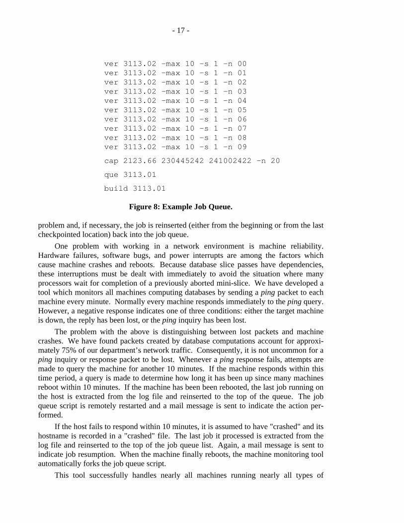
Figure 8 displays an example job queue. Note that the build cannot start until theque is completed. Rather than let a processor take the build and then wait, we usu-ally insert enough work between such dependencies so that when the build is eventu-ally taken, the que has completed.

5.2. A Day in the Life of a Network Supercomputer

We have used as many as 90 workstations computing simultaneously, and keepingtrack of what has been computed and what problems have arisen can be a difficult andtime-consuming task. Before we developed the tools described in this section, manage-ment of the distributed database calculation required a significant time investment everyday. We needed tools to check the consistency of the work being performed and alert usin the event of an error.

The first check occurs with the job queue shell script. For every job computed, thisscript creates a lock file whose name reflects the job being executed. Upon completionof the job, the shell script checks the output file to determine if the job exited normally.If so, the file is removed; otherwise the file remains as a notice that an unusual cir-cumstance occurred. The output files are then manually inspected for the cause of the

- 17 -

ver 3113.02 -max 10 -s 1 -n 00ver 3113.02 -max 10 -s 1 -n 01ver 3113.02 -max 10 -s 1 -n 02ver 3113.02 -max 10 -s 1 -n 03ver 3113.02 -max 10 -s 1 -n 04ver 3113.02 -max 10 -s 1 -n 05ver 3113.02 -max 10 -s 1 -n 06ver 3113.02 -max 10 -s 1 -n 07ver 3113.02 -max 10 -s 1 -n 08ver 3113.02 -max 10 -s 1 -n 09

cap 2123.66 230445242 241002422 -n 20

que 3113.01

build 3113.01

Figure 8: Example Job Queue.

problem and, if necessary, the job is reinserted (either from the beginning or from the lastcheckpointed location) back into the job queue.

One problem with working in a network environment is machine reliability.Hardware failures, software bugs, and power interrupts are among the factors whichcause machine crashes and reboots. Because database slice passes have dependencies,these interruptions must be dealt with immediately to avoid the situation where manyprocessors wait for completion of a previously aborted mini-slice. We have developed atool which monitors all machines computing databases by sending a ping packet to eachmachine every minute. Normally every machine responds immediately to the ping query.However, a negative response indicates one of three conditions: either the target machineis down, the reply has been lost, or the ping inquiry has been lost.

The problem with the above is distinguishing between lost packets and machinecrashes. We have found packets created by database computations account for approxi-mately 75% of our department’s network traffic. Consequently, it is not uncommon for aping inquiry or response packet to be lost. Whenever a ping response fails, attempts aremade to query the machine for another 10 minutes. If the machine responds within thistime period, a query is made to determine how long it has been up since many machinesreboot within 10 minutes. If the machine has been been rebooted, the last job running onthe host is extracted from the log file and reinserted to the top of the queue. The jobqueue script is remotely restarted and a mail message is sent to indicate the action per-formed.

If the host fails to respond within 10 minutes, it is assumed to have "crashed" and itshostname is recorded in a "crashed" file. The last job it processed is extracted from thelog file and reinserted to the top of the job queue list. Again, a mail message is sent toindicate job resumption. When the machine finally reboots, the machine monitoring toolautomatically forks the job queue script.

This tool successfully handles nearly all machines running nearly all types of

- 18 -

database computations. The only manual intervention required occurs when our fileserver is rebooted. In this case, a check of all machines is done to ensure no potentialerrors.

The job queue mechanism with automatic restart upon machine reboot is ideal for aset of identical workstations (with identical performance) and no other users on the net-work. Since many workstations we use belong to other faculty and staff members whoare active during the day, a second tool has been developed to monitor these machines foractivity. Whenever activity is detected, the computations are checkpointed and one oftwo actions are taken. If the workstation swap space is large, the process is suspendedand the operating system migrates the process to the swap space. The monitoring toolrestarts the process after 10 minutes of workstation inactivity. If the workstation does nothave sufficient available swap space, the process is terminated, the job reinserted to thetop of the queue, and a mail message is sent to us describing the action taken. A newprocess is then started on the workstation after normal working hours and monitoringresumes at that time.

Since the database structure and the mini-slice breakdown allows us a high degreeof parallelism, we can always productively use additional workstations. At our peak, wehave had 90 machines performing databases computations in the background at lowpriority. The machines are a heterogeneous collection of Sun, SGI, HP, and MIPSworkstations. Using a single job queue list for a diverse variety of machines is infeasiblebecause of varying processor speeds, amount of available RAM per processor, and day-time restrictions for privately owned machines. Consequently, the job queue list hasbeen sub-divided into four separate lists and each machine obtains its work from one ofthe lists. These queues are called prime, non-prime, slow, and small. Works-tations using prime are assumed to be fast, have sufficient memory to handle any jobtype, and are always accessible. This queue contains immediate, high-priority jobs suchas lookup, noio, or que for the database slice being computed. Workstations usingnon-prime are similar to those using prime except daytime restrictions apply. Thus,this queue is fed low priority work during the day and high priority work during eveningsand weekends. All slow workstations with sufficient memory to handle any job type readtheir jobs from slow. This queue usually contains medium to low priority jobs.Finally, machines with restricted amounts of memory (for example 8 megabytes or less)obtain their jobs from small. This queue contains jobs which are low priority andrequire small amounts of memory (principally DoCaptures()).

Another important tool we have developed is addq. Manually adding work to thequeues occasionally introduced errors. To eliminate this, addq takes a computation,breaks it into mini-slices (roughly 10 million positions per slice) and adds it to the workqueue. This utility is invoked with the name of a queue, the work type to be performed,and the database slice to be acted on. For example,

addq p lookup 3113.01

appends

lookup 3113.01 -max 02 -s 1 -n 00lookup 3113.01 -max 02 -s 1 -n 01

to the prime queue for 3113.01 with 17,035,200 positions. In Figure 8, the

- 19 -

verification of 3113.02 was added using addq.

The primary advantage with using job queues has been obtaining nearly 100%machine utilization for our computations. Very few machines sit idle waiting for the lastmini-slice of a dependency to be completed. The job queue, in addition to the the toolsjust described, has also reduced the manual labor required for database computations.Most effort is now spent moving files between disks, archiving files to tape, and planningthe correct order to insert work into the queues to maximize machine utilization.

Appendix C gives a brief summary of the tools used to manage our network super-computer.

5.3. Using a "Real" Supercomputer

Our retrograde analysis program has also been implemented on a shared memorymultiprocessor, the BBN TC2000 [7]. The basic algorithms, and most of the sourcecode, remain the same but the hardware, software and human overheads are different.

On the TC2000, each process of the parallel job is equivalent to a process workingon a mini-slice in the network supercomputer. The entire active and mirror databases arestored in shared memory to eliminate the I/O on those pages. When a process needs toaccess a portion of the databases that is part of a different mini-slice, it can simply do aread from shared memory. As previously, a process can look up the value of a positionin a different mini-slice, but it can only change positions in its own mini-slice. With thenetwork of workstations, the distributed processes operating on the same database use ashared file system to communicate partial results. Each process works on a disjointmini-slice, but as soon as a page is flushed to disk, another parallel process can access thenew results. In effect, the network file system emulates the communication power ofshared memory, albeit with relatively high latency and low bandwidth. Having sharedmemory supported in hardware, as with the TC2000, reduces the high overheads of theworkstation network. Partial results can be used by other processes more readily, thusincreasing the ability to resolve positions more quickly.

Another advantage of a multiprocessor machine is the ease with which parallelprocesses are created and synchronized. The TC2000 is designed to be used as a mul-tiprocessor, therefore the different processes of a parallel job can be started with a singlecommand instead of having to update one or more network job queues. The homogene-ous nature of the TC2000 processors also make process placement a trivial task. Further-more, with the network of workstations, the central scheduling process implicitly syn-chronizes the processes by how and when it initiates them. Only when one iteration ofthe database is complete are processes for the next iteration initiated. There is also theoverhead of starting up new processes in the network environment, but in a sharedmemory multiprocessor the processes can simply synchronize with a barrier mechanismand continue. Processes are not repeatedly initiated and exited which reduces the startupoverheads and also the human overhead of having to manage the job queues.

Clearly, the BBN TC2000 with its dedicated interconnection network, hardwaresupported shared memory and parallel processors mainly offers a performance advantageto the network of workstations. However, the fact that over a hundred parallel processesare available and the fact that the machine is designed to run parallel programs leads to asubstantial performance advantage over a network of dozens of workstations using

- 20 -

specialized software to manage the distributed processes. We do not exclusively use theTC2000 for the database computations because the addition of the network supercom-puter significantly increases our throughput.

6. Conclusions

During the academic term, we have access to 25-30 workstations in our department,mainly machines on professor’s desks and in graduate student laboratories. Thesemachines allow us to compute roughly 300 million database positions per day. The BBNTC2000 and an additional 60 workstations that we get access to between academic termsallow even greater throughput. The overall throughput averages out to 425 million posi-tions per day.

The 4b4w subset of the 8-piece databases is the last database to be computed.Completing the rest of the 8-piece databases is a daunting task. The 186 billion positionsin the 5b3w endgame will take over a year to complete. Completing this is necessarybefore the 5b4w database (1,997,749,399,776 positions) can be computed. Unless addi-tional computing resources and further motivation can be found, it is unlikely we willtackle this task.

When we first started out in 1989, the 5-piece databases seemed an impossible taskgiven the workstation environment that we had. Now the 7-piece databases are a "trivial"problem. The evolution from a single machine, large address space algorithm to a distri-buted solution that minimizes disk space, execution time and I/O operations has taken along time and an enormous effort. Whether it was all worthwhile depends on the out-come of the next Chinook-Tinsley match (tentatively scheduled for 1994) and whetherthe databases we have are sufficient to solve the game of checkers.

Since most of the database construction process is now automated, we could, intheory, let it continue to run and add 300-400 million positions per day to the databases.However, the other users in our computing environment may have something to sayabout that! Instead, the network supercomputer tools we developed for this project willbe applied to other aspects of checkers. For example, our work queues will be modifiedto specify opening positions. In this way, we can distribute the task of building and veri-fying an opening book. As well, when we start trying to solve the game of checkers, wecan use our network supercomputer to solve different subtrees in the search space inparallel.

Acknowledgements

Various people have helped with the databases including Joseph Culberson, BrentKnight, Patrick Lee and Tim Jellard. Norman Treloar and Duane Szafron have beeninstrumental in the development of Chinook. The technical assistance of Steve Sutphenhas been invaluable. Ken Thompson originally constructed the 5-piece databases for us.Access to the BBN TC2000 was provided by the Massively Parallel Computing Initiative(MPCI) at Lawrence Livermore Laboratory. Brent Gorda of MPCI was an invaluablesource of help for us. The sponsorship of Silicon Graphics International made possiblethe first Chinook-Tinsley match and provided us the opportunity to see what the data-bases could do. This research was funded by the Natural Sciences and EngineeringResearch Council of Canada, grant number OGP-8173, and a grant from the University

- 21 -

of Alberta Central Research Fund.

Finally, the cooperation of the faculty, staff and graduate students in the Departmentof Computing Science at the University of Alberta is appreciated. They have toleratedour thirst for machine cycles with very few complaints.

References

1. I. Althofer, Data Compression Using an Intelligent Generator: the Storage of ChessGames as an Example, Artificial Intelligence 52, 1 (1991), 109-114.

2. S.T. Dekker, H.J. van den Jerik and I.S. Herschberg, Complexity Starts at Five,Journal of the International Computer Chess Association 10, 3 (1987), 125-138.

3. R. Gasser, Applying Retrograde Analysis to Nine Men’s Morris, in Heuristic Pro-gramming in Artificial Intelligence II, D.N.L. Levy and D.F. Beal (ed.), Ellis Hor-wood, London, England, 1991, 161-173.

4. H.J. van den Herik and I.S. Herschberg, The Construction of an OmniscientEndgame Data Base, Journal of the International Computer Chess Association 8, 2(1985), 66-87.

5. H.J. van den Herik, I.S. Herschberg and N. Nakad, A Six-Men-Endgame Database:KRP(a2)KbBP(a3), Journal of the International Computer Chess Association 10, 4(1987), 163-180.

6. H.J. van den Herik and I.S. Herschberg, Thompson: Quintets with Variations,Journal of the International Computer Chess Association 16, 2 (1993), 86-90.

7. R. Lake, P. Lu and J. Schaeffer, Using Retrograde Analysis to Solve Large Com-binatorial Search Spaces, in The 1992 MPCI Yearly Report: Harnessing the KillerMicros, E.D. Brooks, B.J. Heston, K.H. Warren and L.J. Woods (ed.), UCRL-ID-107022-92, I Lawrence Livermore National Laboratory, Livermore, CA, 1992,181-188.

8. P. Lu, Parallel Search of Narrow Game Trees, M.Sc thesis, Department of Comput-ing Science, University of Alberta, 1993.

9. D. Michie and I. Bratko, Ideas on Knowledge Synthesis Stemming from theKBBKN Endgame, Journal of the International Computer Chess Association 10, 1(1987), 3-13.

10. J. Schaeffer, J. Culberson, N. Treloar, B. Knight, P. Lu and D. Szafron, A WorldChampionship Caliber Checkers Program, Artificial Intelligence 53, 2-3 (1992),273-290.

11. J. Schaeffer, N. Treloar, P. Lu and R. Lake, Man Versus Machine for the WorldCheckers Championship, AI Magazine 14, 2 28-35.

12. L. Stiller, Group Graphs and Computational Symmetry on Massively ParallelArchitecture, Journal of Supercomputing 5, (1991), 99-117.

13. K. Thompson, Retrograde Analysis of Certain Endgames, Journal of the Interna-tional Computer Chess Association 9, 3 (1986), 131-139.

14. K. Thompson, Chess Endgames Vol. 1, Journal of the International ComputerChess Association 14, 1 (1991), 22.

- 22 -

15. K. Thompson, Chess Endgames Vol. 2, Journal of the International ComputerChess Association 15, 3 (1992), 149.

Appendix A: Algorithms

In this section, the pseudo code for the various algorithms discussed in this paperare given. The code assumes the following routines:

MakeMove( pos, move )In position pos, move is made, leading to a new position stored in pos.

UnMakeMove( pos, move )In position pos, a move is undone, modifying pos back to the state it wasbefore move was played. MakeMove and UnMakeMove are inverses of eachother.

SetupPosition( pos, db, index )Position number index in db is converted to a board position pos.

index = Index( pos )Convert position pos into its unique number index. SetupPosition andIndex are inverses of each other.

numb = CaptureMoves( pos, moves )In position pos, find all the legal capture moves. The number of moves found isreturned in numb, with the moves being stored in the array moves.

numb = NonCaptureMoves( pos, moves )In position pos there are no capture moves. Find all the legal non-capture moves.The number of moves found is returned in numb, with the moves being stored inthe array moves.

SetValue( db, index, value )Set the value of position index in database db to value. Valid values areWIN, LOSS, DRAW and UNKNOWN.

childvalue = GetValue( db, index )In database db, return the value of position index.

mirror = MIRROR( db )MIRROR is a macro that returns the mirror database of db.

NQueue( db, index )Add the position represented by db and index to a queue of positions. Itassumes there is a global variable PositionQueue indexed by QSize which isinitialized to 0. Each addition to the queue increments QSize. This queue is pro-cessed by DoQueue.

DeQueue( db, index )Remove the position from the head of the PositionQueue, returning its data-base in db and position number in index.

convert = Conversion( move )Determine whether move will cause a conversion to a previously computed data-base. Conversion occurs by a capture move, or by advancing the leading checker.

- 23 -

/* Compute(): generic driver routine for database computations. *//* Called with a function of either DoCaptures(), DoWinningMoves(), *//* DoNonCaptures(), DoLookups(), DoNoIo() or DoVerify(). */

Compute( db, fromindex, toindex, function )database db;int fromindex, toindex;void function();{

int index;

for( index = fromindex; index < toindex; index++ ) {function( db, index );

}}

Figure A1: Compute().

/* DoCaptures(): resolve all capture positions */

DoCaptures( db, index )database db;int index;{

int i, value, numb, childvalue, moves[ MAX_MOVES ];position pos;

value = GetValue( db, index );if( value != UNKNOWN )

return;SetupPosition( pos, db, index );numb = CaptureMoves( pos, moves );if( numb == 0 )

return;

value = LOSS;for( i = 0; i < numb; i++ ) {

MakeMove( pos, moves[ i ] );childvalue = GetValue( MIRROR( db ), Index( pos ) );UnMakeMove( pos, moves[ i ] );if( childvalue == LOSS ) {

value = WIN;break;

}if( childvalue == DRAW )

value = DRAW;}SetValue( db, index, value );

}Figure A2: DoCaptures().

- 24 -

/* DoWinningMoves(): extend all losing positions to their predecessor *//* winning positions. */

DoWinningMoves( db, index )database db;int index;{

int i, value, numb, moves[ MAX_MOVES ];position pos;

value = GetValue( db, index );if( value != LOSS )

return;SetupPosition( pos, db, index );numb = NonCaptureMoves( pos, moves );

for( i = 0; i < numb; i++ ) {MakeMove( pos, moves[ i ] );SetValue( MIRROR( db ), Index( pos ), WIN );UnMakeMove( pos, moves[ i ] );

}}

Figure A3: DoWinningMoves().

- 25 -

/* DoNonCaptures(): try to resolve each non-capture position. It may *//* require repeated passes over the data to resolve all the positions. */

DoNonCaptures( db, index )database db;int index;{

int i, value, numb, childvalue, moves[ MAX_MOVES ];position pos;

value = GetValue( db, index );if( value != UNKNOWN )

return;SetupPosition( pos, db, index );numb = NonCaptureMoves( pos, moves );

value = LOSS;for( i = 0; i < numb; i++ ) {

MakeMove( pos, moves[ i ] );childvalue = GetValue( MIRROR( db ), Index( pos ) );UnMakeMove( pos, moves[ i ] );if( childvalue == LOSS ) {

value = WIN;break;

}if( childvalue == DRAW && value != UNKNOWN )

value = DRAW;else if( childvalue == UNKNOWN )

value = UNKNOWN;}if( value != UNKNOWN ) {

SetValue( db, index, value );if( value != DRAW )

NQueue( db, index );}

}Figure A4: DoNonCaptures().

/* DoQueue(): resolve all positions in the PositionQueue and their *//* predecessors. Called with either DoNonCaptures() or DoNoIo(). */

DoQueue( function )void function();{

database db;int index;

while( QSize != 0 ) {DQueue( db, index );function( db, index );

}}

Figure A5: DoQueue().

- 26 -

/* DoLookups(): for each non-capture position, resolve all references *//* to previously computed databases. This pass obviates the need to *//* reference these databases in any subsequent computation (except *//* verification). At the end of this pass, a value of win or loss is *//* accurate, but a draw means the position is either a tie or a win *//* (it cannot be a loss). */

DoLookups( db, index )database db;int index;{

int i, value, numb, childvalue, moves[ MAX_MOVES ], conv;position pos;

value = GetValue( db, index );if( value != UNKNOWN )

return;SetupPosition( pos, db, index );numb = NonCaptureMoves( pos, moves );

value = LOSS;conv = 0;for( i = 0; i < numb; i++ ) {

if( Conversion( moves[ i ] ) == NO )continue;

conv++;MakeMove( pos, moves[ i ] );childvalue = GetValue( MIRROR( db ), Index( pos ) );UnMakeMove( pos, moves[ i ] );if( childvalue == LOSS ) {

value = WIN;break;

}if( childvalue == DRAW )

value = DRAW;}if( conv == numb && value == LOSS ) {

/* Special case where all moves are conversions */SetValue( db, index, LOSS );

}else if( value != LOSS )

SetValue( db, index, value );}

Figure A6: DoLookups().

- 27 -

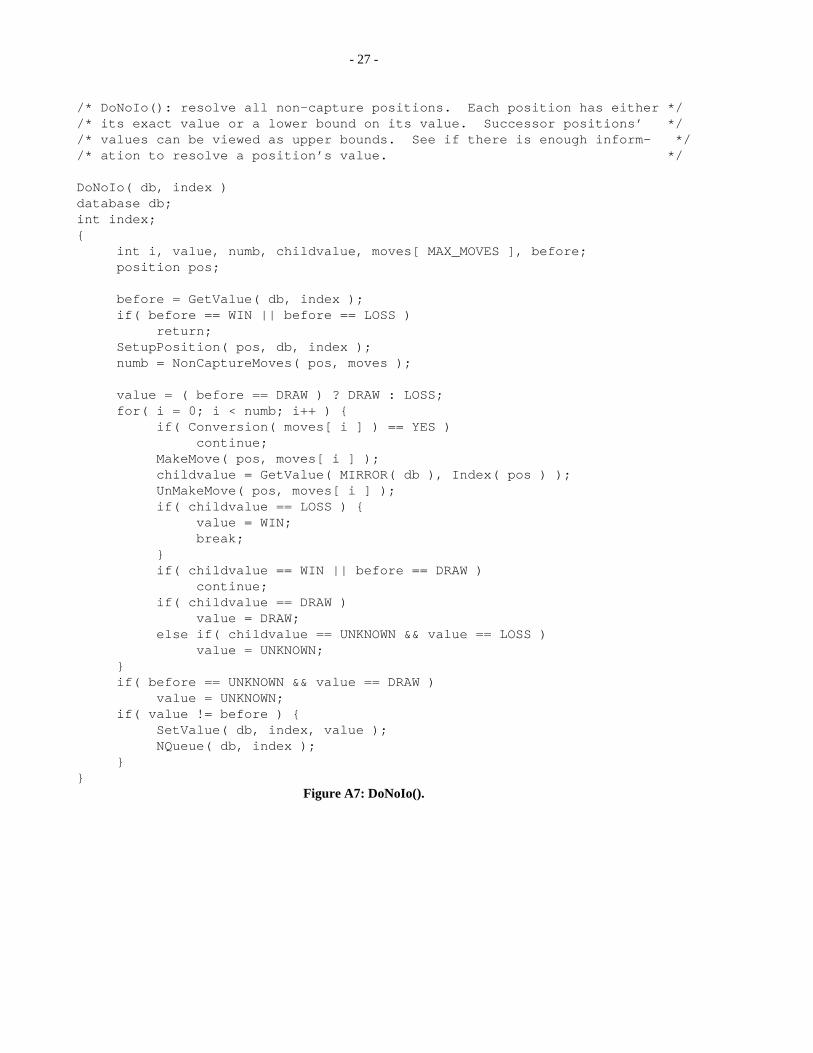
/* DoNoIo(): resolve all non-capture positions. Each position has either *//* its exact value or a lower bound on its value. Successor positions’ *//* values can be viewed as upper bounds. See if there is enough inform- *//* ation to resolve a position’s value. */

DoNoIo( db, index )database db;int index;{

int i, value, numb, childvalue, moves[ MAX_MOVES ], before;position pos;

before = GetValue( db, index );if( before == WIN || before == LOSS )

return;SetupPosition( pos, db, index );numb = NonCaptureMoves( pos, moves );

value = ( before == DRAW ) ? DRAW : LOSS;for( i = 0; i < numb; i++ ) {

if( Conversion( moves[ i ] ) == YES )continue;

MakeMove( pos, moves[ i ] );childvalue = GetValue( MIRROR( db ), Index( pos ) );UnMakeMove( pos, moves[ i ] );if( childvalue == LOSS ) {

value = WIN;break;

}if( childvalue == WIN || before == DRAW )

continue;if( childvalue == DRAW )

value = DRAW;else if( childvalue == UNKNOWN && value == LOSS )

value = UNKNOWN;}if( before == UNKNOWN && value == DRAW )

value = UNKNOWN;if( value != before ) {

SetValue( db, index, value );NQueue( db, index );

}}

Figure A7: DoNoIo().

- 28 -

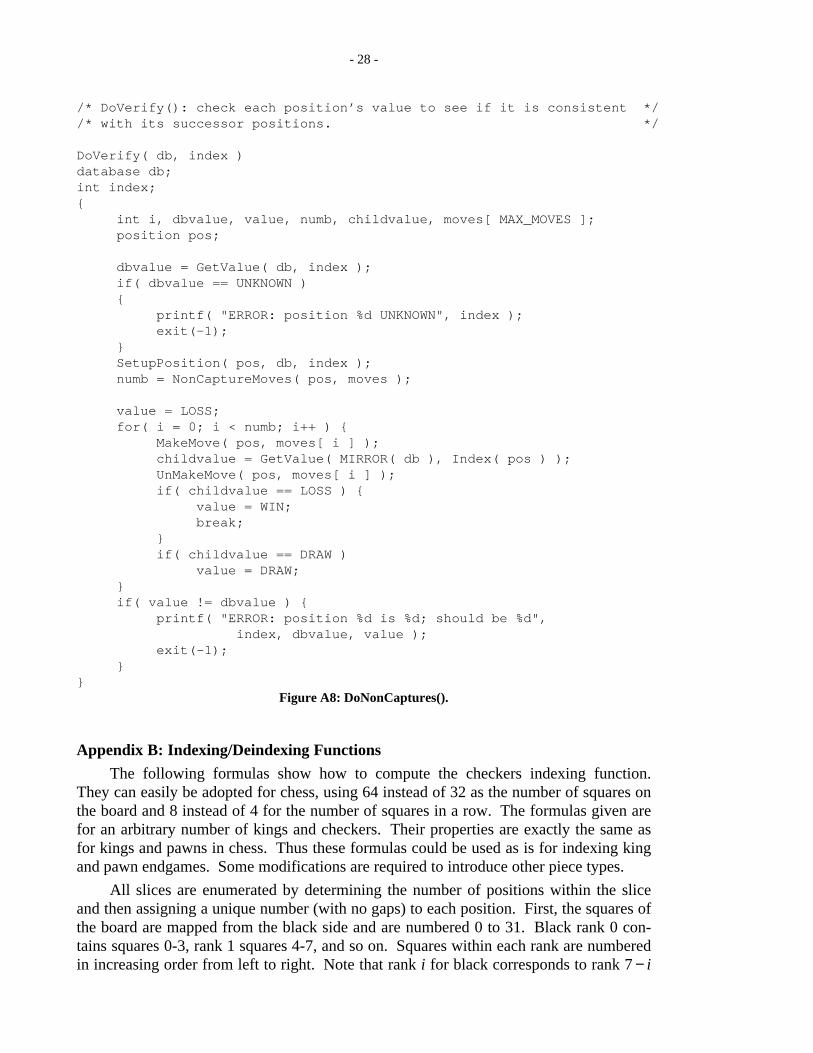
/* DoVerify(): check each position’s value to see if it is consistent *//* with its successor positions. */

DoVerify( db, index )database db;int index;{

int i, dbvalue, value, numb, childvalue, moves[ MAX_MOVES ];position pos;

dbvalue = GetValue( db, index );if( dbvalue == UNKNOWN ){

printf( "ERROR: position %d UNKNOWN", index );exit(-1);

}SetupPosition( pos, db, index );numb = NonCaptureMoves( pos, moves );

value = LOSS;for( i = 0; i < numb; i++ ) {

MakeMove( pos, moves[ i ] );childvalue = GetValue( MIRROR( db ), Index( pos ) );UnMakeMove( pos, moves[ i ] );if( childvalue == LOSS ) {

value = WIN;break;

}if( childvalue == DRAW )

value = DRAW;}if( value != dbvalue ) {

printf( "ERROR: position %d is %d; should be %d",index, dbvalue, value );

exit(-1);}

}Figure A8: DoNonCaptures().

Appendix B: Indexing/Deindexing Functions

The following formulas show how to compute the checkers indexing function.They can easily be adopted for chess, using 64 instead of 32 as the number of squares onthe board and 8 instead of 4 for the number of squares in a row. The formulas given arefor an arbitrary number of kings and checkers. Their properties are exactly the same asfor kings and pawns in chess. Thus these formulas could be used as is for indexing kingand pawn endgames. Some modifications are required to introduce other piece types.

All slices are enumerated by determining the number of positions within the sliceand then assigning a unique number (with no gaps) to each position. First, the squares ofthe board are mapped from the black side and are numbered 0 to 31. Black rank 0 con-tains squares 0-3, rank 1 squares 4-7, and so on. Squares within each rank are numberedin increasing order from left to right. Note that rank i for black corresponds to rank 7 − i

- 29 -

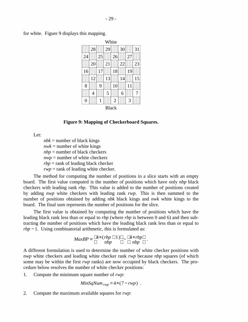
for white. Figure 9 displays this mapping.

0 1 2 3

4 5 6 7

8 9 10 11

12 13 14 15

16 17 18 19

20 21 22 23

24 25 26 27

28 29 30 31

. . . . .. . . . .. . . . .. . . . .. . . . .. . . . .

. . . . .. . . . .. . . . .. . . . .. . . . .. . . . .

. . . . .. . . . .. . . . .. . . . .. . . . .. . . . .

. . . . .. . . . .. . . . .. . . . .. . . . .. . . . .. . . . .. . . . .. . . . .

. . . . .. . . . .

. . . . .

. . . . .. . . . .. . . . .. . . . .. . . . .. . . . .

. . . . .. . . . .. . . . .. . . . .. . . . .. . . . .

. . . . .. . . . .. . . . .. . . . .. . . . .. . . . .. . . . .. . . . .. . . . .

. . . . .. . . . .

. . . . .

. . . . .. . . . .. . . . .. . . . .. . . . .. . . . .

. . . . .. . . . .. . . . .. . . . .. . . . .. . . . .

. . . . .. . . . .. . . . .. . . . .. . . . .. . . . .. . . . .. . . . .. . . . .

. . . . .. . . . .

. . . . .

. . . . .. . . . .. . . . .. . . . .. . . . .. . . . .

. . . . .. . . . .. . . . .. . . . .. . . . .. . . . .

. . . . .. . . . .. . . . .. . . . .. . . . .. . . . .. . . . .. . . . .. . . . .

. . . . .. . . . .

. . . . .

. . . . .. . . . .. . . . .. . . . .. . . . .. . . . .

. . . . .. . . . .. . . . .. . . . .. . . . .. . . . .

. . . . .. . . . .. . . . .. . . . .. . . . .. . . . .. . . . .. . . . .. . . . .

. . . . .. . . . .

. . . . .

. . . . .. . . . .. . . . .. . . . .. . . . .. . . . .

. . . . .. . . . .. . . . .. . . . .. . . . .. . . . .

. . . . .. . . . .. . . . .. . . . .. . . . .. . . . .. . . . .. . . . .. . . . .

. . . . .. . . . .

. . . . .

. . . . .. . . . .. . . . .. . . . .. . . . .. . . . .

. . . . .. . . . .. . . . .. . . . .. . . . .. . . . .

. . . . .. . . . .. . . . .. . . . .. . . . .. . . . .. . . . .. . . . .. . . . .

. . . . .. . . . .

. . . . .

. . . . .. . . . .. . . . .. . . . .. . . . .. . . . .

. . . . .. . . . .. . . . .. . . . .. . . . .. . . . .

. . . . .. . . . .. . . . .. . . . .. . . . .. . . . .

Black

White

Figure 9: Mapping of Checkerboard Squares.

Let:nbk = number of black kingsnwk = number of white kingsnbp = number of black checkersnwp = number of white checkersrbp = rank of leading black checkerrwp = rank of leading white checker.

The method for computing the number of positions in a slice starts with an emptyboard. The first value computed is the number of positions which have only nbp blackcheckers with leading rank rbp. This value is added to the number of positions createdby adding nwp white checkers with leading rank rwp. This is then summed to thenumber of positions obtained by adding nbk black kings and nwk white kings to theboard. The final sum represents the number of positions for the slice.

The first value is obtained by computing the number of positions which have theleading black rank less than or equal to rbp (where rbp is between 0 and 6) and then sub-tracting the number of positions which have the leading black rank less than or equal torbp − 1. Using combinatorial arithmetic, this is formulated as:

MaxBP = nbp4×(rbp + 1 )

− nbp4×rbp

.

A different formulation is used to determine the number of white checker positions withnwp white checkers and leading white checker rank rwp because nbp squares (of whichsome may be within the first rwp ranks) are now occupied by black checkers. The pro-cedure below resolves the number of white checker positions:

1. Compute the minimum square number of rwp:

MinSqNum rwp = 4×( 7 − rwp) .

2. Compute the maximum available squares for rwp:

- 30 -

MaxAvail rwp = 4×(rwp + 1 ) .

3. For each black checker configuration with leading checker rank rbp (i.e. for0≤ i < MaxBP):

3.1. Compute the number of squares within white ranks 0 to rwp occupied by blackcheckers:

NumBP = # o f _black_checker_squares≥MinSqNum rwp .

3.2. Subtract from MaxAvail rwp to obtain the actual number of available whitechecker squares:

Avail rwp = MaxAvail rwp − NumBP .

3.3. Compute Avail rwp − 1 .

3.4. Compute the number of white checker positions with leading rank rwp for thisblack checker configuration:

NumWP i = nwpAvail rwp

− nwpAvail rwp − 1

.

3.5. Add this value to the total number of white checker positions:

MaxWP = MaxWP + NumWP i .

Calculations for MaxBK and MaxWK are much simpler because the multi-directional mobility of the kings does not require specifying a leading rank. Hence, thenumber of positions with nbk black kings given nbp black checkers and nwp white check-ers is:

MaxBK = nbk32 − nbp − nwp

,

and the number of positions with nwk white kings given nbp black checkers, nwp whitecheckers, and nbk black kings is:

MaxWK = nwk32 − nbp − nwp − nbk

.

Thus, the total number of positions for the slice is:

NumPos = MaxBP×MaxWP×MaxBK×MaxWK .

The enumeration algorithm initially assigns the nbp black checkers to the black sideof the board on squares (0, 1, ..., nbp − 1). If the leading rank is greater than zero then thelast checker is assigned to the square rbp×4. White checkers are placed on the white sideof the board: (31, 30, ..., 31-(nwp − 1)). Again, if the leading white rank is greater thanzero then the last checker is assigned to the square 31 − (rwp×4 ). Each white checker ischecked for possible conflicts with other pieces already on the board before its square isassigned. If such a conflict is present, the starting white checker square is decremented.Black kings are assigned initial squares of (0, 1, ..., nbk − 1). As with the white checkers,each black king square is checked for possible conflicts. This time, however, a conflict

- 31 -

results in an increment of the starting king square. White kings are handled similarly toblack kings.

Each position is representable by four tuples, one for each set of pieces. These areexpressed as (bp 0 , bp 1 , ... ,bp nbp − 1 ), (wp 0 , wp 1 , ... ,wp nwp − 1 ), (bk 0 , bk 1 , ... ,bk nbk − 1 ),and (wk 0 , wk 1 , ... ,wk nwk − 1 ). The entries in each tuple correspond to square numbersoccupied by their pieces, sorted left to right in increasing order.

The next index for a tuple, Sq i , is determined by scanning left to right and incre-menting the first element satisfying either Sq i < Sq i + 1 − 1, or i = n andSq n < LastSq ( = 32 ). If neither of these two conditions can be met, the last position forthe tuple has been reached. Otherwise, Sq i is checked for piece conflicts and, if neces-sary, incremented again until a vacant square is found. Elements Sq 0 , Sq 1 , ... ,Sq i − 1 arereset to 0, 1, ..., i − 1 and similar conflict checks are made with each.

The tuples are ordered wk, bk, wp, and bp from least significant to most significant.The next position is obtained by incrementing the lowest available element from thelowest significant tuple. If the tuple affected is not the least significant tuple, then alllower ordered tuples are reset.

The deindexing function takes a numerical value and creates the positioncorresponding to this number. Recall from the discussion of the indexing function thevalues MaxBP, MaxWP, MaxBK, MaxWK, and NumWP i . For any index n where0≤n < NumPos, the method to compute the position described by n is generalized as fol-lows:

1. Initialize tuples bp, wp, bk, and wk.

2. Set i = 0.

3. If n < MaxWK then increment tuple wk n times, and exit.

4. If n < MaxBK×MaxWK then increment tuple bk b times where n = (b×MaxWK) + r.Set n = n − (b×MaxWK) and go to Step 3.

5. If n < NumWP i ×MaxBK×MaxWK then increment tuple wp b times wheren = (b×MaxBK×MaxWK) + r. Set n = n − (b×MaxBK×MaxWK) and go to Step 4.

6. Since n≥NumWP i ×MaxBK×MaxWK, tuple bp must be incremented. The numberof times this tuple is incremented is determined by the values NumWP i obtainedwhen the number of positions in the slice was first determined. Note 0≤ i < MaxBP.

6.1. If n≥NumWP i ×MaxBK×MaxWK then increment tuple bp; else go to Step 5.

6.2. Set n = n − (NumWP i ×MaxBK×MaxWK), i = i + 1, and go to Step 6.1.

The above algorithm requires minor modification whenever one (or more) of thetuples is the empty set.

Appendix C: Network Supercomputer

The following shell scripts and files form the basis for our network supercomputer.

Job queue for prime workstations.db.list.p

Job queue for non-prime workstations.db.list.n

- 32 -

Job queue for workstations with less available memory.db.list.m

Job queue for slow workstations.db.list.s

Edit a job list queue file. This script creates a lock file which preventsany other process from editing the specified job queue file while anediting session is in progress.

vidb

Add syntactically correct job entries to a specific job queue.Example: addq p lookup 3113.01

addq

Display status of capture pass for a specified slice.Example: capcheck 3113.01

capcheck

Display status of lookup pass for a specified slice.Example: lookcheck 3113.01

lookcheck

Display status of non-capture pass for a specified slice.Example: noncheck 3113.01

noncheck

Display status of slice verification.Example: vercheck 3113.01

vercheck

List of workstations eligible for computing databases. Each entry hasthe following format:hostname queue_suffix platform_type memory_sizepublic_or_private night_only,where hostname is the workstation name, queue_suffix is one of p, n, m,s and represents the queue the workstation reads its jobs from,memory_size is the amount of available random access memory forpage tables, public_or_private indicates if a database computation onthe workstations should be suspended during normal working hours,and night_only specifies if the database process should run only atnight and on weekends, and be terminated otherwise.

hosts

Display status of active database computations on all workstationslisted in the hosts file.

dbstatus

Start database processes on a target list of workstations. The programchecks the hosts file to find the architecture of each machine, andspawns the appropriate executable. For example, dbstart host1host2 forks a database process on host1 and host2.

dbstart

Monitor a workstation for interactive activity. If activity is detected,either suspend the process until the interactive session is complete, orcheckpoint and terminate the process.

wswatch

Monitor all workstations computing databases for machine crashes andreboots.

wsmonitor