Embed Size (px)
Citation preview

Environment for Development
Discussion Paper Series June 2008 EfD DP 08-22
Soil Conservation and Small-Scale Food Production in Highland Ethiopia
A Stochastic Metafrontier Approach Ha i lese lass ie A Medh in and Gunnar Koumlh l in
Environment for Development
The Environment for Development (EfD) initiative is an environmental economics program focused on international research collaboration policy advice and academic training It supports centers in Central America China Ethiopia Kenya South Africa and Tanzania in partnership with the Environmental Economics Unit at the University of Gothenburg in Sweden and Resources for the Future in Washington DC Financial support for the program is provided by the Swedish International Development Cooperation Agency (Sida) Read more about the program at wwwefdinitiativeorg or contact infoefdinitiativeorg
Central America Environment for Development Program for Central America Centro Agronoacutemico Tropical de Investigaciacuteon y Ensenanza (CATIE) Email centralamericaefdinitiativeorg
China Environmental Economics Program in China (EEPC) Peking University Email EEPCpkueducn
Ethiopia Environmental Economics Policy Forum for Ethiopia (EEPFE) Ethiopian Development Research Institute (EDRIAAU) Email ethiopiaefdinitiativeorg
Kenya Environment for Development Kenya Kenya Institute for Public Policy Research and Analysis (KIPPRA) Nairobi University Email kenyaefdinitiativeorg
South Africa Environmental Policy Research Unit (EPRU) University of Cape Town Email southafricaefdinitiativeorg
Tanzania Environment for Development Tanzania University of Dar es Salaam Email tanzaniaefdinitiativeorg
copy 2008 Environment for Development All rights reserved No portion of this paper may be reproduced without permission of the authors
Discussion papers are research materials circulated by their authors for purposes of information and discussion They have not necessarily undergone formal peer review
Soil Conservation and Small-Scale Food Production in Highland Ethiopia A Stochastic Metafrontier Approach
Haileselassie A Medhin and Gunnar Koumlhlin
Abstract This study adopts the stochastic metafrontier approach to investigate the role of soil conservation
in small-scale highland agriculture in Ethiopia Plot-level stochastic frontiers and metafrontier technology-gap ratios were estimated for three soil-conservation technology groups and a group of plots without soil conservation Plots with soil conservation were found to be more technically efficient than plots without The metafrontier estimates showed that soil conservation enhances the technological position of naturally disadvantaged plots
Key Words Soil conservation technical efficiency metafrontier technology adoption Ethiopia JEL Classification Q12 Q16 L25
Contents
Introduction 1
2 Conceptual Framework 3
21 Efficiency and Its Measurements 4
22 The Stochastic Metafrontier Model 6
23 Estimation of the Stochastic Metafrontier Curve 9
24 A Brief Empirical Review 11
3 Data and Empirical Specification 12
4 Discussion of Results 17
41 Technical Efficiency and Soil Conservation Group Stochastic Frontiers 17
42 Technical Efficiency and Technology Gaps Metafrontier Estimation 25
5 Concluding Remarks 29
References 31
Environment for Development Medhin and Koumlhlin
1
Soil Conservation and Small Scale Food Production in Highland Ethiopia A Stochastic Metafrontier Approach
Haileselassie A Medhin and Gunnar Koumlhlinlowast
Introduction
Agriculture is the fundamental economic activity in Ethiopia It provides livelihoods for more than three-fourths of the countryrsquos population and accounts for half of the gross domestic product The bulk of the agricultural output comes from mainly subsistent small-holders concentrated in the highlands which are home to more than 80 percent of Ethiopiarsquos population (World Bank 2004) Ethiopian highland agriculture is characterized by high dependency on rainfall traditional technology high population pressure and severe land degradationmdashcompounded by one of the lowest productivity levels in the world
According to World Bank (2005) estimates in the period 2002ndash2004 the average yield was 1318 kghectare which is less than 60 percent of other low-income countries and less than 40 percent of the world average There were only three tractors per arable area of 100 square km (The average was 66 tractors for low-income countries generally) Moreover the agricultural value-added per Ethiopian worker during this period was US$ 123 (in 2000 US dollars) while it was $375 for low-income countries and $776 for the whole world (World Bank 2005) As a result Ethiopia has been one of the top food-aid recipients for decades
In the period 1998ndash2000 the inflow of food aid was more than triple that of total commercial imports (WRI 2005) The Ethiopian highlands have some of the most degraded lands in the world (Hurni 1988) According to Swinton et al (2003) over 10 million hectares will not
lowast Haileselassie A Medhin Environmental Economics Policy Forum for Ethiopia Ethiopian Development Research Institute Blue BuildingAddis Ababa Stadium PO Box 2479 Addis Ababa Ethiopia (email) hailaatyahoocom (tel) + 251 11 5 506066 (fax) +251 115 505588 and Gunnar Koumlhlin Department of Economics University of Gothenburg PO Box 640 405 30 Gothenburg Sweden (email) gunnarkohlineconomicsguse (tel) + 46 31 786 4426 (fax) +46 31 7861043 Financial support for this work from Sida (the Swedish International Development and Cooperation Agency) through the Environment for Development (EfD) initiative at University of Gothenburg Sweden is gratefully acknowledged The authors would also like to acknowledge with thanks access to the data collected by the departments of economics at Addis Ababa University and University of Gothenburg through a collaborative research project entitled ldquoStrengthening Ethiopian Research Capacity in Resource and Environmental Economicsrdquo and financed by SidaSAREC
Resources for the Future Medhin and Koumlhlin
2
be able to support cultivation by 2010 Given such complex environmental and technological constraints it is a daunting challenge for development agents to design efficient policies and strategies to boost agricultural productivity in order to keep up with the ever-growing population
Soil and water conservation (SWC) is one of the most important farm technologies for improving agricultural productivity in areas with high land degradation and limited access to modern inputs1 As with any other farm technology SWC is subject to the complexities of farmersrsquo choices That is its successful adoption depends on the nature of the maximization problem each farmer faces Much of the scarce economic literature on SWC is concentrated on this issue of adoption Most of the studies stress the point that expected yield increase is not the only factor farmers take into consideration in their decision on which technology to adopt Additional factors include risk behavior and time preference (Yesuf 2004 Shively 2001 Shiferaw and Holden 1999) land tenure issues (Swinton et al 2003 Alemu 1999) off-farm activities and resource endowment (Grepperud 1995 Shively 2001) yield variability effect (Shively 1999) and public policies and market structure (Diagna 2003 Yesuf et al 2005 Holden et al 2001)
The economics literature investigating the impact of soil and water conservation shows mixed results Using nationwide Ugandan plot-level data Byiringaro and Reardon (1996) found that farms with greater investment in soil conservation had much better land productivity than the average Nyangena (2006) after controlling for plot-quality characteristics that affect the probability of soil conservation investment concluded that soil and water conservation increased the yield of degraded plots in three districts in Kenya
On the other side Kassie (2005) used plot-level data from a high rainfall area in north-western Ethiopia with a long history of soil conservation which indicated that returns from non-conserved plots were higher than from conserved plotsmdasheven for plots with similar endowments He also pointed out the inappropriateness of the technology for the local area as the main reason for the negative effect But he also stressed that although the soil conservation structures affected yield negatively by becoming breeding stations for pests and weeds their advantage as sources of natural grass for fodder could offset their adverse effect Holden et al
1 Nyangena (2006) also notes that inorganic fertilizers could have negative environmental externalities if not properly used
Resources for the Future Medhin and Koumlhlin
3
(2001) too used data from an Ethiopian highland village and found that conservation technologies had no significant positive short-run effect on land productivity Shively (1999) assessed the effect of hedgerow contours relative to conventional tillage practices for low-income farms in the Philippines These results indicated that although hedgerows can increase yield over time they also increased yield variability Given the risk-aversion behavior of poor farmers the study indicated that establishing hedgerows was not necessarily a better production strategy than conventional practices
Two points are worth mentioning about the existing literature on the role of SWC in small-scale highland agriculture First the results are very case specific both in the type of SWC and in the agro-ecological characteristics of the study areas Therefore one cannot generalize about the impact of SWC on agricultural productivity generally Second the divergence of empirical results is partly related to methodological differences which in turn emanates from the desire to establish theoretically sound and empirically efficient methodological approaches
Based on a concept of productivity decomposition this study aims to contribute to the assessment of the role of SWC in small-scale farming Economic theory indicates that productivity change can be decomposed in to two sources change in technology and change in efficiency (Coelli et al 1998) In this terminology ldquotechnological changerdquo means pushing the production possibility frontier (PPF) outward and ldquoimproving efficiencyrdquo means producing as close as possible to the available PPF A vital relationship between the two is that a change in technology can also bring a change in efficiency Most importantly the effect of technological change on efficiency can be positive or negative Hence it can be said that the effect of a SWC technology as observed in yield change is the net effect of the two sources the direct technology effect and the indirect efficiency effect The existing literature on the yield effect of soil conservation does not distinguish between these two sources of productivity change
Decomposing the yield change into technology and efficiency effects could have important policy relevance It has been mentioned above that the application of SWC has shown mixed results with respect to yield Interventions could be better targeted if it were possible to disentangle these results and show in which circumstances the proposed technology is simply inappropriate as opposed to inefficiently utilized
2 Conceptual Framework
The main goal of this study was to apply such a decomposition as just mentioned This task included two steps First plot-level stochastic production functions and technical
Resources for the Future Medhin and Koumlhlin
4
efficiencies were estimated This gave us a chance to examine the determinants of technical efficiency (TE) in relation to SWC Second efficiency gaps were estimated by testing for any technology gaps between plots cultivated under different SWC technologies A careful look into the role of SWC in the nature of the technology gaps accounting for plot characteristics was the core goal of the study
21 Efficiency and Its Measurements
Farrell (1957) proposed that the efficiency of a firm consists of two components technical efficiency (TE) and allocative efficiency (AE) TE is the ability of a firm to obtain maximum output from a given set of inputs Thus technical inefficiency occurs when a given set of inputs produce less output than what is possible given the available production technology Allocative efficiency is the ability of a firm to use the inputs in optimal proportions given their prices and the production technology (see Coelli et al 1998)
A technically inefficient producer could produce the same outputs with less of at least one input or could use the same inputs to produce more of at least one output In short if there is technical inefficiency there is a room to increase output without increasing input amounts at the present level of technology
Farrell (1957) illustrated efficiency measures with the help of diagrams using two types of measures namely input-oriented measures and output-oriented measures Input-oriented measures tell us the amount of input quantity that can be proportionally reduced without changing the output quantities Output-oriented measures tell us the amount of output quantities that can be proportionally expanded without altering the input amounts used The choice is a matter of convenience as both approaches are expected to give similar measures at least theoretically The input-oriented approach is adopted in this study
Figure 1 is a simple representation of the measurement of efficiency using conventional isoquant and isocost diagrams Assume a firm which produces output Y using two inputs X1 and X2 SSrsquo is a set of fully efficient combinations of X1 and X2 which produce a specific amount of output Ymdashan isoquant Similarly AArsquo is a minimum cost input-price ratio or simply an isocost Now assume that the actual input combination point to produce Y is P Clearly the firm is experiencing both technical and allocative inefficiencies The measures can be estimated as follows
OPQP
OPOQ
TE minus== 1 (1)
Resources for the Future Medhin and Koumlhlin
5
Figure 1 Input-Oriented Technical and Allocative Efficiencies
It is easy to see from equation (1) that TE is always between zero and 1 If the firm is fully technically efficient or if it produces on the isoquant OP equals OQmdashwhich makes the value of TE unity As technical inefficiency increases the distance OP increases which pushes the value of TE towards zero
Similarly allocative efficiency (AE) is defined as
OQORAE = (2)
Equation (2) suggests the possible reduction in costs that can be achieved by using correct input proportions or by producing at the point where the isocost line is tangential to the isoquant line Note that it is possible for a technically efficient point to be allocatively inefficient More specifically the extent of TE does not affect the level of allocative efficiency On the other hand an allocatively efficient point is also technically efficient as Qrsquo is the only allocatively efficient input mix to produce Yrsquo
The total economic efficiency (EE) is defined as the product of the two measures TE and AE That is
OPOR
OQOR
OPOQEE =⎟⎟
⎠
⎞⎜⎜⎝
⎛bull⎟⎟
⎠
⎞⎜⎜⎝
⎛= (3)
X1Y
Source Coelli et al (1998)
Resources for the Future Medhin and Koumlhlin
6
The above efficiency measures assume that the underlining production function is known Therefore the estimation of the production is mandatory for the estimation of efficiency measures Throughout the years various methods of estimating production frontiers have been developed for the purpose of predicting reliable efficiency measures These methods vary from deterministic and non-deterministic (stochastic) econometric models to non-econometric models While the stochastic frontier analysis is the most commonly used among the first group data envelopment analysis is the competent representative of the latter group Battese (1992) indicated that stochastic frontier models better fit agricultural efficiency analysis given the higher noise usually experienced in agricultural data The stochastic metafrontier model is a stochastic frontier model designed to incorporate regional and technological differences among firms in an industry In this study we are mainly interested with the measurement of TE
22 The Stochastic Metafrontier Model
As the prefix ldquometardquo indicates the stochastic metafrontier2 is an umbrella of stochastic
production frontiers estimated for groups of firms operating under different technologies Hence it is more instructive if we start with the definition of stochastic production frontier
The stochastic frontier first introduced by Aigner et al (1977) was developed to remedy the constraints of deterministic models mainly the assumption that the production frontier is common to all firms and that inter-firm variation in performance is therefore attributable only to differences in efficiency Foslashrsund et al (1980) also stated that such an assumption ignores the very real possibility that a firmrsquos performance may be affected by factors entirely beyond its control as well as by factors under its control (inefficiency) In general terms a stochastic production frontier can be written as
( ) ( )ii UVii eXfY minus= β jni 21= (4)
where Yi = output of the ith firm Xi = vector of inputs β = vector of parameters Vi = random error term and Ui = inefficiency term
In agricultural analysis the term Vi captures random factors such as measurement errors weather condition drought strikes luck etc (Battese 1992)
3 Vi is assumed to be independently
2 The stochastic metafrontier applied here is mainly adopted from Battese and Rao (2002) Rao et al (2003) and Battese et al (2004)
Resources for the Future Medhin and Koumlhlin
7
and identically distributed normal random variables with constant variance independent of Ui which is assumed to be non-negative exponential or half-normal or truncated (at zero) variables of N(μi σ2) where μi is defined by some inefficiency model (Coelli et al1998 Battese and Rao 2002) This arises from the nature of production andor cost functions The fact that these functions involve the concepts of minimality or maximality puts bound to the dependent variable To allow this most econometric frontiers assume one-sided inefficiency disturbances (Foslashrsund et al 1980)
Another important point here is the choice of the functional form of f () Battese (1992) noted that the translog or Cobb-Douglas production functions are the most commonly used functional forms for efficiency analysis The Cobb-Douglas specification was adopted for this study It is worth noting that each functional form has its own limitations most of which are related to the technical convenience of the functions and is not the result of deliberate empirical hypotheses In this case the robustness and the parametric linearity of the Cobb-Douglas function make it superior over other functional forms (Coelli 1995 Afriat 1972) The use of translog functions may also lead to excessive multicollinearity (Andre and Abbi 1996 Nyangena 2006)
For this application assume that there are j groups of firms in an industry classified according to their regional or organizational differences (or simply based on their ldquotechnologyrdquo) Suppose that for the stochastic frontier for a sample data of nj firms the jth group is defined by
( ) ( )ijij UVijij eXfY minus= β
jni 21= (5)
Assuming the production function is a Cobb-Douglas or translog form this can be re-written as
( ) ( ) ijijijijij UVXUVijij eeXfY minus+minus == ββ jni 21= (6)
3 One would argue that attributing rainfall and moisture differentials as error elements in a region known for its high dependence on rainfall and severe droughts excludes relevant variables It is a reasonable argument Unfortunately the data used in this study are not endowed with such variables However we firmly believe that as far as efficiency and productivity differentials are concerned this will have a limited impact on the results for two reasons First the data deal with areas of similar geo-climatic characteristics Second the study uses cross-sectional data Therefore it is more likely that rainfall and drought variations would affect efficiency and productivity evenly
Resources for the Future Medhin and Koumlhlin
8
We can soon see the advantage of such a representation Think now about the ldquooverallrdquo stochastic frontier of the firms in the industry without stratifying them into groups Such a frontier can be written as
( ) ( ) iiiii UVXUVii eeXfY minus+minus == ββ ni 21= sum= jnn (7)
Equation (7) is nothing but the stochastic metafrontier function The super-scripts differentiate the parameters and error terms of the metafrontier function from the group-level stochastic functions Note that Yi and Xi remain the same the only difference here is that separate samples of output and inputs of different groups are pooled into a single sample The metafrontier equation is considered to be an envelope function of the stochastic frontiers of the different groups This indicates that we can have two estimates of the TE of a firm with respect to the frontier of its group and with respect to the metafrontier
Mathematically iUi eTE minus= and
iUi eTE minus= respectively
The parameters of both the group frontiers and the metafrontier can be estimated using the method of maximum likelihood estimation After estimating β and β it is expected that the deterministic values Xijβ and Xiβ should satisfy the inequality Xijβ le Xiβ because Xiβ is from the metafrontier According to Battese and Rao (2002) this relationship can be written as
Xi
Xij
1 Ui
Ui
Vi
Vi
ee
ee
ee
minus
minus
sdotsdot= β
β
(8)
Equation (8) simply indicates that if there is a difference between the estimated parameters of a given group and the metafrontier it should arise from a difference in at least one of the three ratios namely the technology gap ratio (TGR) the random error ratio (RER) and the technical efficiency ratio (TER) That is
)(Xi
Xij
i
iUi
UiViVi
Vi
Vi
iXi
i TETE
eeTERande
eeRERe
eeTGR
iequiv=equiv=equiv= minus
minusminusminusminus ββ
β
β
(9)
The technology gap ratio indicates the technology gap for the given group according to currently available technology for firms in that group relative to the technology available in the who industry Note that this assumes all groups have potential access to the best available technology in the industry The TGR and the TER can be estimated for each individual firm
Note from our previous graphical presentation that 0 lt TEi le 1 and 0 lt TEi le 1 It also should be the case that TEi le TEi That is given that the frontier function of the group
Resources for the Future Medhin and Koumlhlin
9
containing firm i is enveloped by the metafrontier function the TE of firm i relative to the metafrontier is at least lower than that of relative to the group frontier Hence the TER is expected to be greater than or equal to unity
The random error ratio is not observable because it is based on the non-observable disturbance term Vi Therefore as far as estimation is concerned equation (8) can be rewritten as
iiUi
Ui
TERTGRee
ee
times=sdot= minus
minus
Xi
Xij
1 β
β
(10)
Combining (9) and (10) gives
ii TGRTETEi
times= (11)
Thus from equation (11) the TE relative to the metafrontier function is the product of the TE relative to the group frontier and the TGR of the technology group This is a very important identity in the sense that it enables us to estimate to what extent the efficiency (hence productivity) of a given firm or group of firms could be increased if it adopted the best available technology in the industry In our case we used this approach to estimate the technology gap between plots with and without soil conservation and investigate the role of different soil conservation practices in defining the technology of farm plots
23 Estimation of the Stochastic Metafrontier Curve
The metafrontier curve is an envelope of the stochastic frontier curves of the technology groups under discussion If each technology group has at least one firm which uses the best technology in the industry (ie if the TGR for the firm is 1) the metafrontier would be the curve connecting these best-practice firms from all groups In cases where no single firm of a given group qualifies for the best technology requirement the stochastic frontier of the group would lie below the metafrontier curve Stochastic frontiers for groups 2 and 4 in figure 2 are examples of this case
Resources for the Future Medhin and Koumlhlin
10
Figure 2 The Stochastic Metafrontier Curve
In reality all production points of the group stochastic frontiers may not lie on or below the metafrontier That is there could be outlier points to group stochastic frontiers (that is why they are stochastic) which could be also outliers to the metafrontier This indicates that estimating the metafrontier demands the very definition of the metafrontier as an assumption That is it assumes that all production points of all groups are enveloped by the metafrontier curve Therefore given the coefficients of group production functions output values and input values estimating the metafrontier is simply the search for the meta coefficients that result in a curve which best fits to the tangent points of the frontier group production functions with best technology firms
According to Battese et al (2004) for a Cobb-Douglas production function (or any function log-linear in parameters) β the metafrontier can be estimated using a simple optimization problem expressed as
Minimize Xrsquoβ
Subject to Xiβ le Xiβ (12)
In equation 12 Xrsquo is the row vector of means of all inputs for each technology group β is the vector group coefficients and β is the vector of meta coefficients we are looking for This is simply a linear programming problem Each plotrsquos production point will be an equation line in a sequence of simultaneous equation with an unknown right hand side variable Note that βs are
S frontier for Group1
S frontier for Group 2
S frontier for Group 4
The metafrontier curve Output Y
Inputs X
S frontier for Group 3
Resources for the Future Medhin and Koumlhlin
11
the maximum likelihood coefficients of the group stochastic frontier from our FRONTIER 414
estimations The constraint inequality is nothing but the envelope assumption we pointed out above
Once we obtain the solutions to out linear programming problem (βs) it is easy to calculate the TGRs and metafrontier technical efficiencies From equation (9) we know that
Xi
Xij
β
β
eeTGRi = and from equation (11) we have ii TGRTETE
itimes= Note that the TEi is already
estimated in our group stochastic frontiers
24 A Brief Empirical Review
A number of studies have investigated the TE of agriculture in various countries Helfand and Levine (2004) assessed the relationship between farm size and efficiency for Brazilian farmers using the data envelopment analysis and found that the relationship is more quadratic than the usual inverse linear relationship It also indicated that type of tenure access to institutions and modern input use have a significant relationship with efficiency differences Coelli and Battese (1996) used a stochastic frontier analysis for three villages in India Their results indicated that farm size age of household head and education are positively related with TE Battese at al (1996) found the same results for four agricultural districts of Pakistan On the other hand Bravo-Utreta and Evenson (1994) although they found significant levels of inefficiency for peasant farmers in Paraguay found no clear relationship of the high inefficiency with the determinants
Very few studies have assessed the relationship of soil conservation and efficiency In their TE analysis of potato farmers in Quebec Amara et al (1998) found that efficient farmers were most likely to invest in soil conservation Yoa and Liu (1998) assessed the TE of 30 Chinese provinces Their results showed that efficiency differentials were significantly related to the ldquodisaster indexrdquo which included physical characteristics such as soil water and infrastructure Irrigation was also found to have positive effect on TE
In the Ethiopian case Admassie and Heindhues (1996) found a positive relationship between TE and fertilizer use Seyum et al (1998) compared farmers within and outside the Sasakowa-Global 2000 project which primarily provided extension and technical assistance for
4 FRONTIER 41 is a software commonly used to estimate production frontiers and efficiency
Resources for the Future Medhin and Koumlhlin
12
farmers Their results showed that farmers participating in the project performed better Abrar (1998) pointed out that farm size age household size and off-farm income are the major determinants of TE in highland Ethiopia
To our knowledge no study has used the metafrontier approach to investigate agricultural efficiency in Ethiopia More importantly we have not found any other study that has used the metafrontier approach to assess the role soil conservation technologies in improving agricultural productivity
3 Data and Empirical Specification
The study is based on the Ethiopian Environmental Household Survey data collected by the departments of economics at Addis Ababa University and University of Gothenburg and managed by the Environmental Economics Policy Forum for Ethiopia (EEPFE) The survey covers six weredas
5 of two important highland zones in the Amhara Region in north Ethiopia Given the similarity of the socio-economic characteristics of the survey areas with other highland regions we believe that the results of the study can be used to comment on policies that aim to increase the productivity of highland small scale agriculture in Ethiopia
Due to the huge coverage of the data set in terms of crop type and land management activity the study focused on two major crop types (teff
6 and wheat) and three main soil conservation activities namely stone bund terracing soil bund terracing and bench terracing It should be noted that even though this data was dropped in the analysis part plots with other soil conservation types were also included in estimating the metafrontier efficiency estimates for the sake of methodological accuracy
The core motive for the need of the metafrontier approach to estimating efficiency is the expectation that plots under different soil conservation practices operate under different technologies If that is the case the traditional way of estimating efficiency by pooling all plots into the same data set may give biased estimates as plots with better technology will appear more efficient This indicates that one needs to test for the feasibility of the traditional approach before adopting the metafrontier That is we should test whether indeed plots under different
5 Wereda is the name for the second lowest administrative level in Ethiopia The lowest is kebele 6 Teff is a tiny grain used to make Ethiopiarsquos most common food item injera The grain has many variants based on its color
Resources for the Future Medhin and Koumlhlin
13
soil conservation practices have regularities in technical efficiency that make it useful to analyze them as different technologies In the meantime we will call them technology groups
As in former studies that applied the metafrontier approach this study uses the likelihood ratio test (LRT) To perform the LRT separate estimations should be performed for each technology group followed by an estimation of the pooled data
7
Teff and wheat crops were grouped according to the type of soil conservation applied in the 2002 main harvest season As can be seen from table 1 there are seven SWC technology groups The first four groups are the emphasis of this paper The stochastic frontier will have two major parts estimated simultaneously the production function and the technical effects While the first part estimates the coefficients of the farm inputs and the attached inefficiency the second part assesses the relationship between the estimated inefficiency and any expected determinants
This indicates that we have two sets of variables inputs and (efficiency) determinants Except for seed the inputs are described in table 1 for each group and for the pooled data The determinants include plot characteristics household characteristics market characteristics and social capital that are expected to affect the extent of TE Table 2 holds the details
Some input variables like fertilizer and manure have zero values for some plots As the model requires input and output values to be converted into logarithms dummy variables which detect such values were included in the production function This means the production function part of the model has two additional variables fertilizer dummy and manure dummy Hence 8 input and 23 determinant coefficients were estimated for each technology group While we identified the input coefficients as βi we identified the determinant coefficients as δi
7 The test compares the values of the likelihood functions of the sum of the separate group estimations and the pooled data In a simple expression the value of the likelihood-ratio test statistic (λ) equals -2ln[L(H0)] - ln[L(H1)] where ln[L(H0)] is the value of the log-likelihood function for the stochastic frontier estimated by pooling the data for all groups and ln[L(H1)] is the sum of the values of the log likelihood functions of the separate groups (Greene 2003)
Environment for Development Medhin and Koumlhlin
14
Table 1 SWC technology Groups
Technology Group Variable Min Max Mean Std
dev Var Technology Group Variable Min Max Mean Std
dev Var
Yield(kgha) 688 1097293 103587 98143 96321166 Yield(kgha) 1324 1726384 125140 120168 1444035
Labor(days) 190 28400 3861 3010 90620 Labor(days) 600 20800 4516 2707 7331
Traction(days) 25 6000 574 577 3337 Traction(days) 100 3600 756 433 18804
Fertilizer(ETB) 00 54900 2499 7726 597056 Fertilizer(ETB) 00 92200 4319 12055 145332
None
(667 plots)
Manure(kg) 00 620000 4179 30540 9327222
Contour furrowing
(473 plots)
Manure(kg) 00 805005 4337 41247 170132
Yield(kgha) 6018 809160 95576 92267 85132708 Yield(kgha) 20415 527798 143205 91721 841267
Labor(days) 350 31700 4897 4186 175293 Labor(days) 1300 10900 4421 2172 47173
Traction(days) 25 2600 479 409 1676 Traction(days) 100 4500 811 462 2131
Fertilizer(ETB) 00 48850 2066 6382 407389 Fertilizer(ETB) 00 50100 6544 14232 202552
Stone bunds
(357 plots)
Manure(kg) 00 93000 5803 15255 2327220
Contour plowing
(97 plots)
Manure(kg) 00 214668 5186 26964 727034
Yield(kgha) 6018 474422 81532 66799 4462131 Yield(kgha) 3833 299154 97934 63159 398906
Labor(days) 750 25900 3980 3742 140054 Labor(days) 850 24900 4563 4086 16691
Traction(days) 50 3600 523 461 2127 Traction(days) 100 1900 484 343 1176
Fertilizer(ETB) 00 25100 1416 4885 238694 Fertilizer(ETB) 00 50100 2716 8530 72766
Soil bunds
(98 plots)
Manure(kg) 00 68934 3726 12440 1547751
Others
(85 plots)
Manure(kg) 00 1760010 28189 191180 3654970
Yield(kgha) 994 397472 94379 63597 40446414 Yield(kgha) 688 1726384 107602 99643 992862
Labor(days) 700 21000 4796 3501 122585 Labor(days) 190 31700 4342 3303 10921
Traction(days) 50 5700 699 695 4832 Traction(days) 25 6000 615 514 2637
Fertilizer(ETB) 00 28000 2874 6963 484894 Fertilizer(ETB) 00 92200 3057 9180 84270
Manure(kg) 00 243335 6496 27313 7460520 Manure(kg) 00 1760010 5770 50430 254318
Bench terraces
(106 plots)
Notes Std dev = standard deviation ha = hectare ETB = Ethiopian birr US$ 1 = ETB 85 Oxen days
Pooled
(1883 plots)
Notes Std dev = standard deviation ha = hectare ETB = Ethiopian birr US$= ETB 85 Oxen days
Resources for the Future Medhin and Koumlhlin
15
Table 2 Definition of Variables
Part 1 Production function
Part 2 Technical effects function
Plot output and inputs Plot characteristics Household characteristics Social capital
LnOutput natural logarithm of kg output
plotage plot age (years that the household cultivated the plot)
Malehh dummy for sex of household head (1 if male 0 if female)
deboD dummy for Debo participation (1 if yes 0 if no)
LnLand natural logarithm of hectare plot area
plotdishome distance from home (minutes of walking)
Agehh age of household head in years
trust number of people the household trusts
LnLabor natural logarithm of labor (person days)
hireD hired labor use dummy (1 if used 0 otherwise)
Educhh years of schooling attended by household head
assi-inD dummy for any assistance received from neighbors (1 if yes 0 if no)
LnTraction natural logarithm of animal traction (oxen days)
Plot Slope meda as a base case Hhsize total family size of the household
assi-outD dummy for any assistance forwarded to neighbors (1 if yes 0 if no)
LnSeed natural logarithm kg seed
dagetD dummy for daget (1 if daget 0 otherwise)
mainacthh dummy for main activity of the household head (1 if farming 0 otherwise)
LnFert natural logarithm of fertilizer applied (ETB)
hillyD dummy for hilly (1 if hilly 0 otherwise)
Offarm total income earned off farm throughout the year
LnMan natural logarithm of manure (kg)
gedelD dummy for gedel (1 if gedel 0 otherwise)
Liv-value total value of livestock owned by the household
fertD dummy for fertilizer use (1 if used 0 otherwise)
LemD dummy for soil quality (1 if lem 0 otherwise)
Farmsize total farm size cultivated by the household in hectares
ManD dummy for manure use (1 if used 0 otherwise)
Cultivation arrangement own cultivation as a base case
Distownm distance to the nearest town in walking minutes
sharecD dummy for share cropping (1 if share cropped 0 otherwise)
rentD dummy for rented plot (1 if rented 0 otherwise)
irrigD irrigation dummy (1 if irrigated 0 otherwise)
Environment for Development Medhin and Koumlhlin
16
The mathematical expressions of the two parts of the stochastic frontier to be estimated are
(the production function)
)exp(
lnlnlnlnlnlnln
ijijijojijoj
ijojijojijojijojijojijojij
UVmanDFertD
manfertseedtractionlaborlandOutput
minus+++
+++++=
ββ
ββββββ
(13)
and the technical effects function (where μi is the mean level of technical inefficiency8 for plot i
in technology group j calculated from (13)
ijijjijjijjijjijj
ijjijjijjijjijjijj
ijjijjijjijjijjijj
ijjijjijjijjijjijjojij
eplotsidhiredDhillyDgedelDdagetD
lemDirrigDrentDsharecDplotageinDassi
outDassitrustdeboDdistownfarmsizevalueliv
offarmmainactDhhsizeeduchhagehhmalehh
ωδδδδδ
δδδδδδ
δδδδδδ
δδδδδδδμ
++++++
+++++minus+
minus+++++minus+
++++++=
hom2322212019
181716151413
121110987
654321
(14)
(wij is a random error term)
For each technology group equations (13) and (14) are (simultaneously) estimated using FRONTIER 41 In addition to the β and δ coefficients the TE of each plot and the log-likelihood functions are also estimated The pooled data are also estimated in the same manner The pooled estimation is critical to the formation of the metafrontier as one should perform the log likelihood test described above
If the LRT gives a green light for use the metafrontier the next step is estimating the stochastic metafrontier function This is done in accordance with the approach discussed in the second chapter Note that in our model we have 8 inputs 7 groups and 1883 plots
The Mathematica 51 software was used to solve the linear programming problem and estimate the meta coefficients Once we estimated the meta coefficients it was easy to calculate the TGR and metafrontier efficiency of each plot in each technology group Besides getting more precise estimates of TE a major emphasis of this study was to assess the extent of the technology-based productivity differential especially between the first four soil conservation groups in table 3 if any It should be noted that the fact that the LRT signals for the use the
8 μi is discussed in appendix 1 together with the maximum likelihood estimation of TE
Resources for the Future Medhin and Koumlhlin
17
metafrontier approach does not guarantee that some groups have better technology than others That is even if the test indicates plots with different soil conservation technologies cannot be pooled into the same frontier model it does not necessarily guarantee that some conservation technologies have better productivity than others Neither does it guarantee that technology gaps if any are only because of soil conservation as plot technology also constitutes many other factors some related to soil conservation adoption
4 Discussion of Results
Productivity change is caused by efficiency andor technology change If the production process of farm plots involves technical inefficiency this means that there is room for improving productivity at the presently available technology at least in the short run But an important point in the technology-efficiency paradigm of productivity change is that technology change may affect the level of efficiency either positively or negatively Therefore a careful analysis of any effect of technology on efficiency is important as it may give a clue to why some technologies that are efficient in controlled environments fail and why others happen to be surprisingly effective when they are applied in the real world The hypothesis is that the hidden change in efficiency because of the technological change may be the reason In this section our main emphasis is looking into the relationship of SWC and the determinants of TE
41 Technical Efficiency and Soil Conservation Group Stochastic Frontiers
Table 3 summarizes the maximum likelihood coefficient estimates of the stochastic production for the different technology groups including the pooled data Most of the estimates are positive and significantly different from zero Note that the parameter estimates of the pooled data are still relevant for the production function even if the LRT rejects the pooled representation That is technological variability within the pooled representation will only bias the TE estimates not the production function coefficient estimates
Plots cultivated under all SWC technologies experience a considerable level of technical inefficiency An important point is that plots without any SWC technology are the least efficient ones with a TE of 0654 At this stage we cannot conclude that plots with SWC have higher productivity than plots without SWC because they have higher TE Such comparison is valid only if we are sure that the two groups operate at similar technology or if the pooled
Resources for the Future Medhin and Koumlhlin
18
Table 3 Coefficients of the Production Function (βs)
Coefficient (t-ratio)
Variable None Soil bunds Stone bunds Bench terraces Pooled
β0
Land
Labor
Traction
Seed
Fertilizer
Manure
Fertilizer use dummy
Manure use
dummy
42487 (204663)
03496 (80103)
02794 (59290)
02081 (53726)
02502 (103058)
-00878
(-15757)
00613 (11711)
04230
(16245)
-02959 (-11053)
43130 (47752)
03436 (16600)
02992
(16263)
-01521 (-11041)
02678 (28847)
-01332
(-06145)
01215 (06437)
05533
(05705)
-03893 (-03986)
45430 (147057)
02377 (43778)
01408 (25056)
03395 (60643)
01193 (31099)
-00248
(-01993)
01541 (23833)
00575
(00973)
-06386 (-18279)
58685 (63162)
07310 (38998)
00082
(004735)
03116 (24046)
00866
(12983)
00381 (03887)
-01461
(-10644)
-00605 (-01352)
11504
(14711)
43618 (354124)
03149 (120299)
02290 (84113)
02071 (82998)
02337 (155857)
-00038 (01303)
00235
(08208)
00410 (02832)
00116
(00758)
Note significant at α=005 significant at α=010
representation is valid The value of the LRT statistic (λ) was calculated to be 37124 The Chi-square test at 8 degrees of freedom
9 shows that this is significant at α = 0005
10 That is the null
hypothesis that says the pooled stochastic estimation is a correct representation of the data is
9 The number of restrictions is 8 10 χ2
8 (0005) = 21 9550 lt 37124 the null hypothesis is rejected
Resources for the Future Medhin and Koumlhlin
19
rejected Most importantly it means that there is a significant technology differential among the four groups in tables 3 and 4
Table 4 Mean TE and the Coefficients of the Technical Effects Function
Variable None Soil bunds Stone bunds Bench Pooled
Mean TE 065498 077971 067615 068731 067825
δ0 -68962 (-26735)
10558 (01076)
-26569 (-20452)
-43708 (-04472)
-96613 (-43111)
Sex (dummy) 12182 (17476)
-68500 (-08454)
37077 (27549)
12617 (01090)
19818 (37108)
Age 04960 (29383)
-00433 (-03123)
02702 (23600)
04447 (22635)
06415 (48117)
Education -01404 (-04175)
-03246 (-04170)
-01417 (-03791)
-11810 (-10822)
-03474 (-18520)
Household size 02045 (05005)
-00578 (-00520)
-01968 (-03112)
25167 (16728)
07351 (27342)
Main activity -10623 (-17635)
21261 (02891)
-19442 (-25224)
-107105 (-10941
-94019 (-29118)
Off-farm income -00079 (-18921)
-00007 (-03056)
00060 (18899)
-00134 (-14099)
-00064 (-33254)
Livestock value -00059 (-29657)
-00030 (-12549)
-00009 (-08834)
-00034 (-18948)
-00077 (-51426)
Total farm size 21393 (18683)
12783 (040663)
-02277 (-11995)
10189 (30714)
2992 (36047)
Distance to town 00788 (27139)
00312 (04933)
00023 (09623)
-00263 (-04255)
00578 (39907)
Debo participationDagger 82177 (25904)
32114 (06406)
-12368 (-20270)
-17534 (-16866)
69117 (30831)
Trust 29064 (27174)
30401 (12716)
01730 (14437)
-64733 (-24664)
37709 (45653)
Assistance out 08798 (02607)
10665 (01862)
-01818 (-02995)
24201 (02505)
28926 (14989)
Assistance in 54461 (16355)
16024 (02104)
-43070 (-08385)
124097 (15060)
14449 (46344)
Plot age 00060 (0583)
-00979 (-04386)
-00145 (-071709
-1211 (-37327)
-02968 (-34008)
Sharecropping 9664 (25071)
-46274 (-04832)
-06560 (-10204)
-23074 (-23585)
-32866 (-13362)
Resources for the Future Medhin and Koumlhlin
20
Variable None Soil bunds Stone bunds Bench Pooled
Rented plot 27494 (23689)
-10917 (-10949)
-157011 (-13543)
00000 (00000)
117834 (12167)
Irrigated plot -177503 (-15543)
00000 (0000)
45381 (04590)
-66149 (-05901)
-37566 (-03838)
Soil quality (lem) 11298 (29373)
15768 (04681)
29235 (12979)
-11431 (-18835)
13511 (13065)
Slope 1 daget 30071 (08710)
-24226 (-07463)
-40035 (-13371)
-58438 (-10081)
-3894 (-27111)
Slope 2 gedel -63602 (-22769)
-99969 (-11439)
41842 (04611)
61680 (06356)
-10658 (-23365)
Slope 3 hilly -58643 (-18064)
11059 (01106)
14767 (25999)
00000 (00000)
376805 (42053)
Hired labor -8983 (-17960)
49991 (05541)
-14379 (-19570)
-87772 (-11541)
-15919 (-41300)
Plot distance to home
0066 (16809)
00162 (01325)
00915 (11901)
01137 (06470)
00594 (24021)
Sigma 2 20749 (39425)
2720 (29200)
8152 (53933)
59377 (36084)
28803 (59753)
Gamma 8977
(358897) 19297
(06559) 7453
(112089) 77165 (90520)
9260 (891217)
Notes significant at α=005 significant at α=010 Dagger See text footnote 13 for explanation of Debo project
Before going to the details it is important to clarify what the TE-determinant estimates in table 4 mean and what they do not mean in the presence of the technology differential First the estimates of the pooled specification in the last column are not valid any more Second any TE-based productivity comparison among the four groups should take into account that they operate at different technologies That is the fact that a given group has higher TE does not mean it is more productive it means plots under this group operate closer to their group technology frontier which is not necessarily the best technology frontier compared to frontiers of other groups Therefore productivity comparisons are only possible only if we know the position of group frontiers relative to the best technology frontier in all groups or the metafrontier Third the fact that the LRT rejects the pooled representation of the data does not invalidate the group-level TE and inefficiency-determinant coefficient estimates It only limits their universality across technology groups group technical inefficiency for plot i in technology group j is the
Resources for the Future Medhin and Koumlhlin
21
potential improvement in output if plot i applies the best technology available in group j This will be clear when we look into our results from the stochastic metafrontier estimation
In addition to technology differentials it is also appropriate to deal with non-random forces that could affect output The user cost of SWC is one such variable Even though our data failed to give a precise estimate some studies have shown that SWC investment takes away a considerable amount of land and labor from the production process (Shiferaw and Holden 1998 2001) In our case the land cost is important because the plot size in our production functions does not account for the land lost to SWC While the labor input in our production function does not include the amount of labor spent on constructing or maintaining SWC structures
11 the land
lost is included in the plot size as if it was used for crop cultivation Hence every unit of output lost for every unit of land occupied by SWC structures is detected as if it resulted from technical inefficiency This indicates that TE estimates for plots with SWC could be understated by our model which stresses our point that conserved plots are more efficient that unconserved ones Such downward effect is more interesting if the land cost varies with plot characteristics as will soon be shown
Some plot characteristics in the technical-effects model could be related to SWC adoption In such cases the results for each technology group should be interpreted by taking into consideration the adoption effect If for example the probability of a plot being conserved increases with the plot having an attribute i and ifmdashfor a given SWC technologymdashefficiency is positively related with attribute i it is logical to suspect that it is the presence of attribute imdashnot soil conservationmdashthat is the reason for better efficiency On the other hand if we have no evidence that the probability of soil conservation is related to the plot having attribute i and if efficiency is positively related to attribute i for conserved plots and negatively related (or not related at all) for unconserved plots we can conclude that SWC positively affects efficiency through attribute i However it should be noted that our results may not be as simple as these clean cases This is mainly because efficiency may have various determinants which could have different effects for each conservation technology
12
11 The labor cost of SWC does not affect the TE estimate even though it could affect allocative efficiency (AE) estimates 12 This indicates that SWC could also be related to AE Although the analysis of AE is far from the scope of this study we believe that it would have helped in understanding the complex relationship between soil conservation and productivity Among other things this requires good price data
Resources for the Future Medhin and Koumlhlin
22
It is assumed that farmers tend to conserve highly degraded plots relative to less degraded plots In the absence of detailed soil composition data plot slope and soil quality are the best proxies for soil degradation That is if highly degraded plots have a better chance of being conserved the probability of SWC could also increase with steep slope and poorer soil quality Table 5 shows the results of the Mann-Whitney test
Table 5 Mann-Whitney Test for Plot Slope and Soil Quality
Plot characteristics Hypotheses Z-value P-value
Slope H0 SlopeC = SlopeU
H1 SlopeC gt SlopeU 66104 0000
Soil quality H0 Soil QC = Soil QU
H1 Soil QC lt Soil QU 14220 00778
Notes C= conserved U = unconserved significant at α = 001 significant at α = 01
The null hypothesis that conserved plots and unconserved plots have similar slopes is rejected at a very high level of significance That is steeper plots have a higher likelihood of being conserved in the study areas As for soil quality the null hypothesis that plots with poorer soil quality get more attention in the conservation decision is not rejected unless we are willing to accept a 778-percent room for error The moderate decrease in soil quality with soil conservation could be because of the negative correlation between slope and soil quality (with partial correlation of 0158) In other words conservation decision may be based on expected vulnerability to soil erosion rather on increasing soil quality More specifically farmers may choose to conserve better soil-quality plots on steep slopes rather than low quality plots on moderate slopes This is certainly worth investigating in further research as it could be related to the risk aversion of poor farmers invest to protect what you already have rather than upgrade what is lost
We now have evidence that plot slope is related to the conservation decision This indicates that any relationship between slope and efficiency should be assessed critically taking into consideration that conserved plots have steeper slopes From table 4 steep slope is negatively related to technical inefficiency for plots without SWC On the other hand steep slope is positively related to technical inefficiency for plots with stone bunds while there is no significant relationship for the other SWC technologies That is unconserved steep plots have better TE than conserved steep plots An explanation for this could be the relationship between the per-hectare land cost of SWC with plot slope Shiferaw and Holden (2001) estimated that for
Resources for the Future Medhin and Koumlhlin
23
a 45-percent increase in slope the per-hectare land lost for SWC increases by 900 percent The fact that the negative impact of such high land costs on output is now absorbed as technical inefficiency justifies the result that the positive relationship of high slope and TE disappears with the introduction of SWC
High soil quality and TE are negatively related for unconserved plots and positively related for plots with bench terraces Furthermore there is no significant relationship for plots with stone bunds and soil bunds That is soil conservation erases or alters the negative relationship of high soil quality and TE This means even though high soil-quality plots have a slightly lower likelihood of being conserved they have higher TE than unconserved high soil-quality plots other things held constant
The relationship between the gender of household heads and TE is surprising The fact that a household is headed by a male is negatively related to TE for unconserved plots and for plots with stone bunds the relationship being stronger in the latter group This is contrary to many studies which showed female-headed households are less efficient than male-headed households Age of household head is also negatively related to efficiency except for plots with soil bunds where there is no significant relationship Education has a non-significant positive relationship with TE for all technology groups Unconserved and stone bund plots cultivated by household heads with farming as a main activity have higher TE The positive relationship is more pronounced in the case of stone bunds Off-farm income has a weak positive relationship with efficiency for plots without soil conservation and a rather weaker negative relationship for stone bund plots Increasing livestock wealth has a small but positive effect on efficiency although it is insignificant for stone and soil bunds Larger total farm size has a negative relationship with efficiency at least for unconserved plots and plots with bench terraces
Plot distance from home has a negative effect on TE for plots without conservation while it has no significant effect for plots with SWC The same is true for distance to the nearest town Sharecropping is negatively related to efficiency for unconserved plots while it has a strong positive relationship for plots with bench terraces Land rental is also negatively related to efficiency for plots without conservation while it has a non-significant relationship for conserved plots Plots which employed hired labor have better efficiency especially if they have stone bund structures
Resources for the Future Medhin and Koumlhlin
24
Unconserved plots cultivated by households who participate in Debo13 have lower efficiency while Debo participation is positively related to efficiency for plots with stone bunds and bench terraces It has no significant relationship for plots with soil bunds Unconserved plots cultivated by peasants who trust more people in their neighborhood are also less efficient than conserved plots That is soil conservation alters the negative relationship of higher social capital and efficiency
The above paragraphs indicate that in most cases negative relationships between various plot and household attributes and TE disappear or are reversed in the presence of one of the soil conservation technologies That is for some reason soil conservation positively affects the role of the determinants of efficiency Studying the explicit aspect in which soil conservation affects the role of plot household market characteristics and social capital in determining the level of TE could shed new lights on the economics of soil conservation adoption and productivity analysis This is certainly an attractive area of further research
It is important to note that the fact that conserved plots have higher TE does not necessarily mean they also have higher yield than plots without soil conservation It simply means that the chosen amounts of inputs were used more effectively in the case of conserved plots Table 6 below compares the yield and input values of plots with and without soil conservation The average yield for plots with conservation is significantly lower than that of plots without conservation even though the difference is not significant Conserved plots use a significantly higher amount of labor than unconserved plots while the latter use a higher amount of seed The differences in manure fertilizer and traction are insignificant
As can be seen in table 6 even though conserved plots have higher TE than unconserved plots they still have lower mean yield One reason for this is the fact that conservation decision is partly based on plot characteristics such as plot slope and soil quality that have a significant impact on yield in their own right Therefore direct yield and input comparisons can only be used to comment on the effect of productivity technologies if plots are homogenous or if the
13 Debo is a non-profit organization focused on helping alleviate extreme poverty in rural Ethiopia It offers a wide range of projects (education agriculture health water development and reforestation plus microcredit and job skills training) implemented with a local non-profit partner Debo Yeerdata Mahiber The agricultural projects work with rural communities ldquoto boost food production promote sustainable environment and overcome povertyrdquo primarily through reforestation to reclaim soil erosion and creation of local nurseries to supply trees See httpdeboethiopiaorgsourceProgramsDeboProgramshtml
Resources for the Future Medhin and Koumlhlin
25
conservation decision is independent of plot characteristics that affect output One point that should be kept in mind is that SWC could be productivity enhancing even if it does not lead to the highest yield simply because it is not the only determinant of yield The discussion of the metafrontier results in the next section elaborates this point
Table 6 Yield and Input Use Comparison
Variable With soil conservation Without soil conservation Difference
Mean Std dev Mean Std dev With-without P-value
Yield (kgh) 92897 83491 103587 98143 -10690 0 0421
Labor (days) 4718 3998 3862 3010 856 00002
Manure (kg) 5571 17761 4180 30540 1391 03309
Fertilizer (ETB) 2105 6271 2499 7727 -394 03594
Traction (oxen days)
528 491 574 578 -046 01391
Seed (kg) 1805 4074 2619 4018 -814 00000
Std dev = standard deviation ETB = Ethiopian birr US$ 1 = ETB 85
42 Technical Efficiency and Technology Gaps Metafrontier Estimation
Table 7 illustrates the results of the metafrontier estimation in combination with the group TE results from table 4 Note that while group technical inefficiency (1 - group TE) for plot i in technology group j is the potential improvement in output if plot i applies the best technology available in group j On the other hand metafrontier technical inefficiency for plot i in technology group j is the potential increase in output if plot i applies the best technology available in all groups The mean TGR for a given group quantifies the average gap between group technology and overall technology The maximum value 1000 indicates that at least one plot in the group uses the best technology available for all groups In other words group frontiers with maximum TGR of 1000 are tangential to the metafrontier curve All group frontiers are tangential to the metafrontier except for bench terraces
Plots with soil bunds have the lowest mean TGR 07806 This simply indicates that even if all soil bund plots attain the maximum technology available for the group they will still be about 219 percent away from the output that they could produce if they used the maximum
Resources for the Future Medhin and Koumlhlin
26
Table 7 Technology Gaps and Metafrontier TE
Technology group Variable Minimum Maximum Mean Std dev
None TGRa
Meta TE Group TE
06134 01133 01133
10000 098682 098687
09494 062061 065497
009972 017301 016892
Stone bunds TGR Meta TE Group TE
06558 012449 014898
10000 093073 093080
09539 064607 067614
008123 018027 017716
Soil bunds TGR Meta TE Group TE
05264 015034 017841
10000 092095 097442
07806 060600 077970
008881 015727 019122
Bench terraces
TGR Meta TE Group TE
05499 013687 013688
09999 094353 094464
09629 065748 068733
008881 020040 020766
TGR= technology gap ratio Std dev = standard deviation
technology available in the whole sample The significantly lower value of the meta TE relative to the all higher group TE says exactly the same Although the potential improvement in output relative to the best technology available for soil bund plots is only 2203 percent it is 394-percent relative to the best technology available for all groups Note that meta TE is not a real efficiency measure per se It only quantifies by how much output could be increased if a given group had the best technology We can say a plot is technically inefficient only if it fails to produce the maximum attainable output using the technology it applies
Now it is time to face the big question is SWC a good technology
From table 7 we see that plots without SWC have no significant technology gap relative to plots with three SWC technologies Moreover it is plots with soil bunds which have the highest technology gap (lowest TGR) From these results it seems logical to conclude that plots with SWC do not use higher technology than plots without soil conservation This may seem a short answer to the big question but it is not Actually it is not an answer to the question at all Our question is not whether plots with SWC have better technology it is whether SWC is a good
Resources for the Future Medhin and Koumlhlin
27
technology Given that a given plotrsquos technology constitutes other factors14
in addition to soil conservation it could be the case that plots without SWC have a better composite technology than plots with soil conservationmdashso soil conservation could still be a good technology
Note that this point is strictly related to our earlier finding that soil conservation adoption is dependent on plot characteristics
15 This means adoption of a given type of SWC technology is
related to a plotrsquos prior composite technology More specifically SWC technology has been shown to be adopted in plots with poor conditions In such cases it is possible that SWC improved the composite technology of conserved plots and that still unconserved plots have a higher composite technology Accordingly we can say that a given type of SWC is a better technology if among others one of the following is satisfied First a given SWC technology is good if conserved plots could have performed worse had they not been conserved Second soil conservation is a good technology if unconserved plots could have performed better had they been conserved
One way to assess these requirements is to start by answering the question of which plots have the best technology These are the plots with a TGR very close to the value 1000 from our metafrontier estimation Studying the technology characteristics of these frontier plots in some detail could shed some light on the role of soil conservation Table 8 is a summary of descriptive values and frequencies of plot characteristics that define the metafrontier technology We have now identified the 147 plots that define the best practice in the 1228 plots that were cultivated under the four technology groups including plots without conservation (which are 543 percent of the sample) Our goal was to look for the role of plot characteristics
16 in making the frontier in
all conservation types That is we were looking for the remaining variables that defined the composite technology besides soil conservation
17
14 Plot characteristics farming equipment and farmer ability are also primary components of the composite technology If plots and their farmers were homogenous we could argue that the difference in technology is only because of soil conservation 15 Plot characteristics could include plot slope and soil quality For simplicity we can identify them as natural technologies 16 Usage of modern inputs such as fertilizer also affects the composite technology But in table 6 we found that there is no significant difference in the use of such inputs between conserved and unconserved plots 17 If we had plot-level moisture data table 8 could have been more informative as moisture level would certainly affect the technology position of plots
Resources for the Future Medhin and Koumlhlin
28
Table 8 Characteristics of Best Technology Plots
Soil conservation technology ( share)
Plot characteristics None Stone bunds
Soil bunds
Bench terraces All best
share in whole sample
Plot slope
Meda Dagetma Gedel Hilly
773 227
0 0
679 250 71 0
250 500 250
0
833 83 83 0
728 231 41 0
700 267 24 07
Soil quality
Lem Lem-tef Tef Other Chora
413 307 280 00 00
482 375 143 00 00
250 500 250 00 00
250 750 00 00 00
422 374 204 00 00
401 416 180 01 01
Soil type
Black Red Brown Gray Black red
240 693 13 13 27
464 500 00 18 18
0 1000 00 00 00
833 167 00 00 00
367 585 7 14 20
420 511 2 19 29
Crop type
White teff Mixed teff Blackred teff Wheat
147 147 187 520
196 18
143 643
500 00
250 250
500 83
167 250
204 88
170 537
298 121 243 338
Number of frontier plots 75 56 4 12 147
Total number of plots 667 357 98 106 1228
Percentage of frontier plots
112 156 40 113 119
The roles of plot slope soil quality soil type and crop type were examined Of the plots which define the best practice 728 percent have a plain slope (meda) and 394 percent have no soil conservation technology It is worth noting that the share of steep plots in the best-practice group increases with SWC technology This could be again related to the fact that steep plots have a higher likelihood of being conserved This finding asserts our earlier proposition that the positive relationship between plot slope and technical inefficiency emanates from the increase of land costs of SWC with slope In all conservation types good soil-quality plots also have a better share in the best technology group
Corrected to its sample share the stone bunds group has the highest number of plots that qualify as best practice (156 percent) Bench terraces none and soil bunds follow with shares of
Resources for the Future Medhin and Koumlhlin
29
113 percent 112 percent and 40 percent respectively This indicates that even though the ldquono SWCrdquo group has the highest share of plots in the sample space soil conservation groups outrank it in the best plots scenario except for soil bunds In general the shares of different plot-characteristics categories in the best-practice group are closely related to their shares in the sample space An important lesson from table 8 is that plots with a better soil and topographic condition (advantaged plots) with or without SWC still define the best technology in the survey areas SWC helps by giving this chance to disadvantaged plots Therefore soil conservation is a good technology
The metafrontier approach also gives new insights into the group-level TE estimates The best example in our case is the soil bunds group Although plots cultivated with soil bunds have a relatively lower technology their high mean group TE indicates their lower technology is used more efficiently than plots cultivated with other soil conservation practices If in some way their high efficiency is related to their soil bund terraces we cannot conclude that soil bund terracing is a bad technology as there could be a net productivity improvement Output of plots with soil bunds could be increased by 4 percent if they were conserved with stone bunds because of better technology On the other hand the output of plots with stone bunds could be increased by 104 percent if they were conserved by soil bunds because of higher efficiency Therefore the output of plots with stone bunds could be increased by 64 percent if they were conserved by soil bunds because what matters is the net effect of technology and efficiency Soil bund terracing is an even better technology
5 Concluding Remarks
This study used the newly developed metafrontier approach to assess the TE of small-scale food production in the Ethiopian highlands at plot level with the main goal of investigating the role of soil conservation technology in enhancing agricultural productivity To this end stochastic frontiers were estimated for four technology groups including a group of plots without soil conservation technology After testing for technological difference among groups a metafrontier production curve was estimated and technology gaps of each plot in each technology group were calculated
The group stochastic frontier estimations showed that plots with SWC technologies are relatively more efficient than plots without soil conservation For all soil-conservation technology groups mean technical inefficiency was regressed against various plot household market and social capital variables The results indicated that the likelihood of negative technical effects decreased with SWC Most importantly these results showed that that the
Resources for the Future Medhin and Koumlhlin
30
decomposition of the yield productivity effect of farm technologies into technology and efficiency effects has indeed relevant policy values Studying the aspects in which a given SWC affects efficiency could shed some light on why laboratory-effective SWC technologies underperform in the real world
The stochastic metafrontier estimation showed that plots cultivated under different SWC practices operated under different technologies This indicated that efficiency estimations that fail to take into account such technology differential could lead to biased results An in-depth look at the characteristics of best-practice plots showed that SWC is a major part the definition of a plotrsquos composite technology but not all of it While advantaged plots dominated the frontier regardless of their conservation status disadvantaged plots made it to the frontier with the help of SWC Hence SWC proved to be good technology
The stochastic metafrontier proved to be promising in the quest for a methodology that enables us to assess the productivity effect of new technologies or policy interventions in industries with heterogeneous firms and production strategies In small-scale agriculture the prevalence of such heterogeneities is usually the biggest challenge in the design of policies and strategies to boost productivity For example a critical issue in the economics of SWC in small-scale agriculture is the matching problem which SWC practice fits which agro-economic environment One can approach this problem by performing a metafrontier estimation on plots under different agro-economic environments and identifying which SWC works better with which plothousehold attributes
Resources for the Future Medhin and Koumlhlin
31
References
Abrar S 1998 ldquoIdentifying the Sources of Technical Inefficiency of Ethiopian Farmers Using the (Single Stage) Stochastic Frontier Inefficiency Modelrdquo Working Papers series Addis Ababa Ethiopia Addis Ababa University Department of Economics
Admassie A and F Heindhues 1996 ldquoEstimation of Technical Efficiency of Smallholder Farmers in the Central Highlands of Ethiopiardquo Ethiopian Journal of Agricultural Economics 1(1) 19ndash35
Afriat SN 1972 ldquoEfficiency Estimation of Production Functionsrdquo International Economic Review 13(3) 568ndash95
Aigner DJ CAK Lovell and P Schmidt 1977 ldquoFormulation and Estimation of Stochastic Frontier Production Function Modelsrdquo Journal of Econometrics 6 21ndash37
Alemu T 1999 ldquoLand Tenure and Soil Conservation Evidence from Ethiopiardquo PhD diss (92) School of Economics and Commercial Law University of Gothenburg Sweden
Amara N N Traoreacute R Landry and R Romain 1998 ldquoTechnical Efficiency and Farmersrsquo Attitudes toward Technological Innovation The Case of the Potato Farmers in Quebecrdquo Canadian Journal of Agricultural Economics 47(1) 31ndash43
Croppenstedt A and A Mammo 1996 ldquoAn Analysis of the Extent of Technical Efficiency of Farmers Growing Cereals in Ethiopia Evidence from Three Regionsrdquo Ethiopian Journal of Economics 5(1) 39ndash62
Battese G E 1992 ldquoFrontier Production Functions and Technical Efficiency A Survey of Empirical Applications in Agricultural Economicsrdquo Agricultural Economics 7 185ndash208
Battese GE and TJ Coelli 1988 ldquoPrediction of Firm-Level Technical Efficiencies with Generalized Frontier Production Function and Panel Datardquo Journal of Econometrics 38 387ndash99
Battese GE SJ Malik and MA Gill 1996 ldquoAn Investigation of Technical Inefficiencies of Production of Wheat Farmers in Four Districts of Pakistanrdquo Journal of Agricultural Economics 47 37ndash49
Battese GE and DSP Rao 2002 ldquoTechnology Gap Efficiency and a Stochastic Metafrontier Functionrdquo International Journal of Business and Economics 1(2) 1ndash7
Resources for the Future Medhin and Koumlhlin
32
Battese GE DSP Rao and CJ OrsquoDonnell 2004 ldquoA Metafrontier Production Function for Estimation of Technical Efficiencies and Technology Gaps for Firms Operating under Different Technologiesrdquo Journal of Productivity Analysis 21 91ndash103
Bravo-Ureta BE and RE Evenson 1994 ldquoEfficiency in Agricultural Production The Case of Peasant Farmers in Eastern Paraguayrdquo Agricultural Economics 10 27ndash37
Byiringiro F and T Reardon 1996 ldquoFarm Productivity in Rwanda Effects of Farm Size Erosion and Soil Conservation Investmentrdquo Agricultural Economics 15 127ndash36
Coelli T 1995 ldquoRecent Developments in Frontier Modeling and Efficiency Measurementrdquo Australian Journal of Agricultural Economics 39(3) 219ndash45
Coelli T and GE Battese 1996 ldquoIdentification of the Factors Which Influence the Technical Inefficiency of Indian Farmersrdquo Australian Journal of Agricultural Economics 40(2) 103ndash28
Coelli T DSP Rao C OrsquoDonnell and GE Battese 1998 An Introduction to Productivity and Efficiency and Productivity Analysis 2nd ed New York Springer
Diagana B 2003 ldquoLand Degradation in Sub-Saharan Africa What Explains the Widespread Adoption of Unsustainable Farming Practicesrdquo Draft working paper Department of Agricultural Economics and Economics Montana State University Bozeman MT
Farrell MJ 1957 ldquoThe Measurement of Productive Efficiencyrdquo Journal of Royal Statistical Society Series A 120 253ndash81
Foslashrsund FR CAK Lovell and P Schmidt 1980 ldquoA Survey of Frontier Production Functions and Their Relationship to Efficiency Measurementrdquo Journal of Econometrics 13 5ndash25
Greene WH 2003 Econometric Analysis 5th ed Upper Saddle River NJ Prentice Hall
Grepperud S 1995 ldquoSoil Conservation and Government Policies in Tropical Areas Does Aid Worsen the Incentives for Arresting Erosionrdquo Agricultural Economics 12(1995) 12ndash140
Griffiths WE RC Hill and GG Judge 1993 Learning and Practicing Econometrics Hoboken NJ John Wiley amp Sons Inc
Helfand SM and ES Levine 2004 ldquoFarm Size and the Determinants of Productive Efficiency in the Brazilian Center Westrdquo Agricultural Economics 31 241ndash49
Resources for the Future Medhin and Koumlhlin
33
Holden S B Shiferaw and J Pender 2001 ldquoMarket Imperfections and Land Productivity in Ethiopian Highlandsrdquo Journal of Agricultural Economics 52(3) 53ndash70
Hurni H 1988 ldquoDegradation and Conservation of the Resources in the Ethiopian Highlandsrdquo Mountain Research and Development 8(23) 123ndash30
Kassie M 2005 ldquoTechnology Adoption Land Rental Contracts and Agricultural Productivityrdquo PhD diss (200520) Norwegian University of Life Sciences Arings
Nyangena W 2006 ldquoEssays on Soil Conservation Social Capital and Technology Adoptionrdquo PhD diss (148) School of Business Economics and Law University of Gothenburg Sweden
Seyum ET GE Battese and EM Fleming 1998 ldquoTechnical Efficiency and Productivity of Maize Producers in Eastern Ethiopia A Study of Farmers within and outside the Sasakowa-Global 2000 Projectrdquo Agricultural Economics 19 341ndash48
Shiferaw B and S Holden 1998 ldquoResource Degradation and Adoption of Land Conservation Technologies in the Ethiopian Highlands A Case Study in Andit Tid North Shewardquo Agricultural Economics 18 233ndash47
mdashmdashmdash 1999 ldquoSoil Erosion and Smallholdersrsquo Conservation Decisions in the Highlands of Ethiopiardquo World Development 27(4) 739ndash52
mdashmdashmdash 2001 ldquoFarm-Level Benefits to Investments for Mitigating Land Degradation Empirical Evidence for Ethiopiardquo Environment and Development Economics 6 336ndash59
Shively GE 1999 ldquoRisks and Returns from Soil Conservation Evidence from Low-Income Farms in the Philippinesrdquo Agricultural Economics 21 53ndash67
mdashmdashmdash 2001 ldquoPoverty Consumption Risk and Soil Conservationrdquo Journal of Development Economics 65 267ndash90
Swinton SM and B Gebremedhin 2003 ldquoInvestment in Soil Conservation in Northern Ethiopia The Role of Land Tenure Security and Public Programsrdquo Agricultural Economics 29 69ndash84
World Bank 2004 World Development Report 2004 Making Services Work for Poor People Washington DC World Bank
mdashmdashmdash 2005 ldquoWorld Development Indicators 2005rdquo Washington DC World Bank
Resources for the Future Medhin and Koumlhlin
34
WRI (World Resources Institute) 2005 ldquoWRI Downloadable Datasetsrdquo httparchivewriorgpubsdatasetscfmSortBy=1
Yesuf M 2004 ldquoRisk Time and Land Management under Market Imperfections Application to Ethiopiardquo PhD diss (139) School of Economics and Commercial Law University of Gothenburg Sweden
Yesuf M and J Pender 2005 ldquoDeterminants and Impacts of Land Management Technologies in the Ethiopian Highlands A Literature Reviewrdquo Draft paper Environmental Economics Policy Forum in Ethiopia (EEPFE) Addis Ababa Ethiopia and International Food Policy Research Institute (IFPRI) Washington DC httpwwwefdinitiativeorgresearchprojectsproject-repositoryeconomic-sector-work-on-poverty-and-land-degradation-in-ethiopia
Yoa S and Z Liu 1998 ldquoDeterminants of Grain Production and Technical Efficiency in Chinardquo Journal of Agricultural Economics 49 171ndash84

Environment for Development Medhin and Koumlhlin
1
Soil Conservation and Small Scale Food Production in Highland Ethiopia A Stochastic Metafrontier Approach
Haileselassie A Medhin and Gunnar Koumlhlinlowast
Introduction
Agriculture is the fundamental economic activity in Ethiopia It provides livelihoods for more than three-fourths of the countryrsquos population and accounts for half of the gross domestic product The bulk of the agricultural output comes from mainly subsistent small-holders concentrated in the highlands which are home to more than 80 percent of Ethiopiarsquos population (World Bank 2004) Ethiopian highland agriculture is characterized by high dependency on rainfall traditional technology high population pressure and severe land degradationmdashcompounded by one of the lowest productivity levels in the world
According to World Bank (2005) estimates in the period 2002ndash2004 the average yield was 1318 kghectare which is less than 60 percent of other low-income countries and less than 40 percent of the world average There were only three tractors per arable area of 100 square km (The average was 66 tractors for low-income countries generally) Moreover the agricultural value-added per Ethiopian worker during this period was US$ 123 (in 2000 US dollars) while it was $375 for low-income countries and $776 for the whole world (World Bank 2005) As a result Ethiopia has been one of the top food-aid recipients for decades
In the period 1998ndash2000 the inflow of food aid was more than triple that of total commercial imports (WRI 2005) The Ethiopian highlands have some of the most degraded lands in the world (Hurni 1988) According to Swinton et al (2003) over 10 million hectares will not
lowast Haileselassie A Medhin Environmental Economics Policy Forum for Ethiopia Ethiopian Development Research Institute Blue BuildingAddis Ababa Stadium PO Box 2479 Addis Ababa Ethiopia (email) hailaatyahoocom (tel) + 251 11 5 506066 (fax) +251 115 505588 and Gunnar Koumlhlin Department of Economics University of Gothenburg PO Box 640 405 30 Gothenburg Sweden (email) gunnarkohlineconomicsguse (tel) + 46 31 786 4426 (fax) +46 31 7861043 Financial support for this work from Sida (the Swedish International Development and Cooperation Agency) through the Environment for Development (EfD) initiative at University of Gothenburg Sweden is gratefully acknowledged The authors would also like to acknowledge with thanks access to the data collected by the departments of economics at Addis Ababa University and University of Gothenburg through a collaborative research project entitled ldquoStrengthening Ethiopian Research Capacity in Resource and Environmental Economicsrdquo and financed by SidaSAREC
Resources for the Future Medhin and Koumlhlin
2
be able to support cultivation by 2010 Given such complex environmental and technological constraints it is a daunting challenge for development agents to design efficient policies and strategies to boost agricultural productivity in order to keep up with the ever-growing population
Soil and water conservation (SWC) is one of the most important farm technologies for improving agricultural productivity in areas with high land degradation and limited access to modern inputs1 As with any other farm technology SWC is subject to the complexities of farmersrsquo choices That is its successful adoption depends on the nature of the maximization problem each farmer faces Much of the scarce economic literature on SWC is concentrated on this issue of adoption Most of the studies stress the point that expected yield increase is not the only factor farmers take into consideration in their decision on which technology to adopt Additional factors include risk behavior and time preference (Yesuf 2004 Shively 2001 Shiferaw and Holden 1999) land tenure issues (Swinton et al 2003 Alemu 1999) off-farm activities and resource endowment (Grepperud 1995 Shively 2001) yield variability effect (Shively 1999) and public policies and market structure (Diagna 2003 Yesuf et al 2005 Holden et al 2001)
The economics literature investigating the impact of soil and water conservation shows mixed results Using nationwide Ugandan plot-level data Byiringaro and Reardon (1996) found that farms with greater investment in soil conservation had much better land productivity than the average Nyangena (2006) after controlling for plot-quality characteristics that affect the probability of soil conservation investment concluded that soil and water conservation increased the yield of degraded plots in three districts in Kenya
On the other side Kassie (2005) used plot-level data from a high rainfall area in north-western Ethiopia with a long history of soil conservation which indicated that returns from non-conserved plots were higher than from conserved plotsmdasheven for plots with similar endowments He also pointed out the inappropriateness of the technology for the local area as the main reason for the negative effect But he also stressed that although the soil conservation structures affected yield negatively by becoming breeding stations for pests and weeds their advantage as sources of natural grass for fodder could offset their adverse effect Holden et al
1 Nyangena (2006) also notes that inorganic fertilizers could have negative environmental externalities if not properly used
Resources for the Future Medhin and Koumlhlin
3
(2001) too used data from an Ethiopian highland village and found that conservation technologies had no significant positive short-run effect on land productivity Shively (1999) assessed the effect of hedgerow contours relative to conventional tillage practices for low-income farms in the Philippines These results indicated that although hedgerows can increase yield over time they also increased yield variability Given the risk-aversion behavior of poor farmers the study indicated that establishing hedgerows was not necessarily a better production strategy than conventional practices
Two points are worth mentioning about the existing literature on the role of SWC in small-scale highland agriculture First the results are very case specific both in the type of SWC and in the agro-ecological characteristics of the study areas Therefore one cannot generalize about the impact of SWC on agricultural productivity generally Second the divergence of empirical results is partly related to methodological differences which in turn emanates from the desire to establish theoretically sound and empirically efficient methodological approaches
Based on a concept of productivity decomposition this study aims to contribute to the assessment of the role of SWC in small-scale farming Economic theory indicates that productivity change can be decomposed in to two sources change in technology and change in efficiency (Coelli et al 1998) In this terminology ldquotechnological changerdquo means pushing the production possibility frontier (PPF) outward and ldquoimproving efficiencyrdquo means producing as close as possible to the available PPF A vital relationship between the two is that a change in technology can also bring a change in efficiency Most importantly the effect of technological change on efficiency can be positive or negative Hence it can be said that the effect of a SWC technology as observed in yield change is the net effect of the two sources the direct technology effect and the indirect efficiency effect The existing literature on the yield effect of soil conservation does not distinguish between these two sources of productivity change
Decomposing the yield change into technology and efficiency effects could have important policy relevance It has been mentioned above that the application of SWC has shown mixed results with respect to yield Interventions could be better targeted if it were possible to disentangle these results and show in which circumstances the proposed technology is simply inappropriate as opposed to inefficiently utilized
2 Conceptual Framework
The main goal of this study was to apply such a decomposition as just mentioned This task included two steps First plot-level stochastic production functions and technical
Resources for the Future Medhin and Koumlhlin
4
efficiencies were estimated This gave us a chance to examine the determinants of technical efficiency (TE) in relation to SWC Second efficiency gaps were estimated by testing for any technology gaps between plots cultivated under different SWC technologies A careful look into the role of SWC in the nature of the technology gaps accounting for plot characteristics was the core goal of the study
21 Efficiency and Its Measurements
Farrell (1957) proposed that the efficiency of a firm consists of two components technical efficiency (TE) and allocative efficiency (AE) TE is the ability of a firm to obtain maximum output from a given set of inputs Thus technical inefficiency occurs when a given set of inputs produce less output than what is possible given the available production technology Allocative efficiency is the ability of a firm to use the inputs in optimal proportions given their prices and the production technology (see Coelli et al 1998)
A technically inefficient producer could produce the same outputs with less of at least one input or could use the same inputs to produce more of at least one output In short if there is technical inefficiency there is a room to increase output without increasing input amounts at the present level of technology
Farrell (1957) illustrated efficiency measures with the help of diagrams using two types of measures namely input-oriented measures and output-oriented measures Input-oriented measures tell us the amount of input quantity that can be proportionally reduced without changing the output quantities Output-oriented measures tell us the amount of output quantities that can be proportionally expanded without altering the input amounts used The choice is a matter of convenience as both approaches are expected to give similar measures at least theoretically The input-oriented approach is adopted in this study
Figure 1 is a simple representation of the measurement of efficiency using conventional isoquant and isocost diagrams Assume a firm which produces output Y using two inputs X1 and X2 SSrsquo is a set of fully efficient combinations of X1 and X2 which produce a specific amount of output Ymdashan isoquant Similarly AArsquo is a minimum cost input-price ratio or simply an isocost Now assume that the actual input combination point to produce Y is P Clearly the firm is experiencing both technical and allocative inefficiencies The measures can be estimated as follows
OPQP
OPOQ
TE minus== 1 (1)
Resources for the Future Medhin and Koumlhlin
5
Figure 1 Input-Oriented Technical and Allocative Efficiencies
It is easy to see from equation (1) that TE is always between zero and 1 If the firm is fully technically efficient or if it produces on the isoquant OP equals OQmdashwhich makes the value of TE unity As technical inefficiency increases the distance OP increases which pushes the value of TE towards zero
Similarly allocative efficiency (AE) is defined as
OQORAE = (2)
Equation (2) suggests the possible reduction in costs that can be achieved by using correct input proportions or by producing at the point where the isocost line is tangential to the isoquant line Note that it is possible for a technically efficient point to be allocatively inefficient More specifically the extent of TE does not affect the level of allocative efficiency On the other hand an allocatively efficient point is also technically efficient as Qrsquo is the only allocatively efficient input mix to produce Yrsquo
The total economic efficiency (EE) is defined as the product of the two measures TE and AE That is
OPOR
OQOR
OPOQEE =⎟⎟
⎠
⎞⎜⎜⎝
⎛bull⎟⎟
⎠
⎞⎜⎜⎝
⎛= (3)
X1Y
Source Coelli et al (1998)
Resources for the Future Medhin and Koumlhlin
6
The above efficiency measures assume that the underlining production function is known Therefore the estimation of the production is mandatory for the estimation of efficiency measures Throughout the years various methods of estimating production frontiers have been developed for the purpose of predicting reliable efficiency measures These methods vary from deterministic and non-deterministic (stochastic) econometric models to non-econometric models While the stochastic frontier analysis is the most commonly used among the first group data envelopment analysis is the competent representative of the latter group Battese (1992) indicated that stochastic frontier models better fit agricultural efficiency analysis given the higher noise usually experienced in agricultural data The stochastic metafrontier model is a stochastic frontier model designed to incorporate regional and technological differences among firms in an industry In this study we are mainly interested with the measurement of TE
22 The Stochastic Metafrontier Model
As the prefix ldquometardquo indicates the stochastic metafrontier2 is an umbrella of stochastic
production frontiers estimated for groups of firms operating under different technologies Hence it is more instructive if we start with the definition of stochastic production frontier
The stochastic frontier first introduced by Aigner et al (1977) was developed to remedy the constraints of deterministic models mainly the assumption that the production frontier is common to all firms and that inter-firm variation in performance is therefore attributable only to differences in efficiency Foslashrsund et al (1980) also stated that such an assumption ignores the very real possibility that a firmrsquos performance may be affected by factors entirely beyond its control as well as by factors under its control (inefficiency) In general terms a stochastic production frontier can be written as
( ) ( )ii UVii eXfY minus= β jni 21= (4)
where Yi = output of the ith firm Xi = vector of inputs β = vector of parameters Vi = random error term and Ui = inefficiency term
In agricultural analysis the term Vi captures random factors such as measurement errors weather condition drought strikes luck etc (Battese 1992)
3 Vi is assumed to be independently
2 The stochastic metafrontier applied here is mainly adopted from Battese and Rao (2002) Rao et al (2003) and Battese et al (2004)
Resources for the Future Medhin and Koumlhlin
7
and identically distributed normal random variables with constant variance independent of Ui which is assumed to be non-negative exponential or half-normal or truncated (at zero) variables of N(μi σ2) where μi is defined by some inefficiency model (Coelli et al1998 Battese and Rao 2002) This arises from the nature of production andor cost functions The fact that these functions involve the concepts of minimality or maximality puts bound to the dependent variable To allow this most econometric frontiers assume one-sided inefficiency disturbances (Foslashrsund et al 1980)
Another important point here is the choice of the functional form of f () Battese (1992) noted that the translog or Cobb-Douglas production functions are the most commonly used functional forms for efficiency analysis The Cobb-Douglas specification was adopted for this study It is worth noting that each functional form has its own limitations most of which are related to the technical convenience of the functions and is not the result of deliberate empirical hypotheses In this case the robustness and the parametric linearity of the Cobb-Douglas function make it superior over other functional forms (Coelli 1995 Afriat 1972) The use of translog functions may also lead to excessive multicollinearity (Andre and Abbi 1996 Nyangena 2006)
For this application assume that there are j groups of firms in an industry classified according to their regional or organizational differences (or simply based on their ldquotechnologyrdquo) Suppose that for the stochastic frontier for a sample data of nj firms the jth group is defined by
( ) ( )ijij UVijij eXfY minus= β
jni 21= (5)
Assuming the production function is a Cobb-Douglas or translog form this can be re-written as
( ) ( ) ijijijijij UVXUVijij eeXfY minus+minus == ββ jni 21= (6)
3 One would argue that attributing rainfall and moisture differentials as error elements in a region known for its high dependence on rainfall and severe droughts excludes relevant variables It is a reasonable argument Unfortunately the data used in this study are not endowed with such variables However we firmly believe that as far as efficiency and productivity differentials are concerned this will have a limited impact on the results for two reasons First the data deal with areas of similar geo-climatic characteristics Second the study uses cross-sectional data Therefore it is more likely that rainfall and drought variations would affect efficiency and productivity evenly
Resources for the Future Medhin and Koumlhlin
8
We can soon see the advantage of such a representation Think now about the ldquooverallrdquo stochastic frontier of the firms in the industry without stratifying them into groups Such a frontier can be written as
( ) ( ) iiiii UVXUVii eeXfY minus+minus == ββ ni 21= sum= jnn (7)
Equation (7) is nothing but the stochastic metafrontier function The super-scripts differentiate the parameters and error terms of the metafrontier function from the group-level stochastic functions Note that Yi and Xi remain the same the only difference here is that separate samples of output and inputs of different groups are pooled into a single sample The metafrontier equation is considered to be an envelope function of the stochastic frontiers of the different groups This indicates that we can have two estimates of the TE of a firm with respect to the frontier of its group and with respect to the metafrontier
Mathematically iUi eTE minus= and
iUi eTE minus= respectively
The parameters of both the group frontiers and the metafrontier can be estimated using the method of maximum likelihood estimation After estimating β and β it is expected that the deterministic values Xijβ and Xiβ should satisfy the inequality Xijβ le Xiβ because Xiβ is from the metafrontier According to Battese and Rao (2002) this relationship can be written as
Xi
Xij
1 Ui
Ui
Vi
Vi
ee
ee
ee
minus
minus
sdotsdot= β
β
(8)
Equation (8) simply indicates that if there is a difference between the estimated parameters of a given group and the metafrontier it should arise from a difference in at least one of the three ratios namely the technology gap ratio (TGR) the random error ratio (RER) and the technical efficiency ratio (TER) That is
)(Xi
Xij
i
iUi
UiViVi
Vi
Vi
iXi
i TETE
eeTERande
eeRERe
eeTGR
iequiv=equiv=equiv= minus
minusminusminusminus ββ
β
β
(9)
The technology gap ratio indicates the technology gap for the given group according to currently available technology for firms in that group relative to the technology available in the who industry Note that this assumes all groups have potential access to the best available technology in the industry The TGR and the TER can be estimated for each individual firm
Note from our previous graphical presentation that 0 lt TEi le 1 and 0 lt TEi le 1 It also should be the case that TEi le TEi That is given that the frontier function of the group
Resources for the Future Medhin and Koumlhlin
9
containing firm i is enveloped by the metafrontier function the TE of firm i relative to the metafrontier is at least lower than that of relative to the group frontier Hence the TER is expected to be greater than or equal to unity
The random error ratio is not observable because it is based on the non-observable disturbance term Vi Therefore as far as estimation is concerned equation (8) can be rewritten as
iiUi
Ui
TERTGRee
ee
times=sdot= minus
minus
Xi
Xij
1 β
β
(10)
Combining (9) and (10) gives
ii TGRTETEi
times= (11)
Thus from equation (11) the TE relative to the metafrontier function is the product of the TE relative to the group frontier and the TGR of the technology group This is a very important identity in the sense that it enables us to estimate to what extent the efficiency (hence productivity) of a given firm or group of firms could be increased if it adopted the best available technology in the industry In our case we used this approach to estimate the technology gap between plots with and without soil conservation and investigate the role of different soil conservation practices in defining the technology of farm plots
23 Estimation of the Stochastic Metafrontier Curve
The metafrontier curve is an envelope of the stochastic frontier curves of the technology groups under discussion If each technology group has at least one firm which uses the best technology in the industry (ie if the TGR for the firm is 1) the metafrontier would be the curve connecting these best-practice firms from all groups In cases where no single firm of a given group qualifies for the best technology requirement the stochastic frontier of the group would lie below the metafrontier curve Stochastic frontiers for groups 2 and 4 in figure 2 are examples of this case
Resources for the Future Medhin and Koumlhlin
10
Figure 2 The Stochastic Metafrontier Curve
In reality all production points of the group stochastic frontiers may not lie on or below the metafrontier That is there could be outlier points to group stochastic frontiers (that is why they are stochastic) which could be also outliers to the metafrontier This indicates that estimating the metafrontier demands the very definition of the metafrontier as an assumption That is it assumes that all production points of all groups are enveloped by the metafrontier curve Therefore given the coefficients of group production functions output values and input values estimating the metafrontier is simply the search for the meta coefficients that result in a curve which best fits to the tangent points of the frontier group production functions with best technology firms
According to Battese et al (2004) for a Cobb-Douglas production function (or any function log-linear in parameters) β the metafrontier can be estimated using a simple optimization problem expressed as
Minimize Xrsquoβ
Subject to Xiβ le Xiβ (12)
In equation 12 Xrsquo is the row vector of means of all inputs for each technology group β is the vector group coefficients and β is the vector of meta coefficients we are looking for This is simply a linear programming problem Each plotrsquos production point will be an equation line in a sequence of simultaneous equation with an unknown right hand side variable Note that βs are
S frontier for Group1
S frontier for Group 2
S frontier for Group 4
The metafrontier curve Output Y
Inputs X
S frontier for Group 3
Resources for the Future Medhin and Koumlhlin
11
the maximum likelihood coefficients of the group stochastic frontier from our FRONTIER 414
estimations The constraint inequality is nothing but the envelope assumption we pointed out above
Once we obtain the solutions to out linear programming problem (βs) it is easy to calculate the TGRs and metafrontier technical efficiencies From equation (9) we know that
Xi
Xij
β
β
eeTGRi = and from equation (11) we have ii TGRTETE
itimes= Note that the TEi is already
estimated in our group stochastic frontiers
24 A Brief Empirical Review
A number of studies have investigated the TE of agriculture in various countries Helfand and Levine (2004) assessed the relationship between farm size and efficiency for Brazilian farmers using the data envelopment analysis and found that the relationship is more quadratic than the usual inverse linear relationship It also indicated that type of tenure access to institutions and modern input use have a significant relationship with efficiency differences Coelli and Battese (1996) used a stochastic frontier analysis for three villages in India Their results indicated that farm size age of household head and education are positively related with TE Battese at al (1996) found the same results for four agricultural districts of Pakistan On the other hand Bravo-Utreta and Evenson (1994) although they found significant levels of inefficiency for peasant farmers in Paraguay found no clear relationship of the high inefficiency with the determinants
Very few studies have assessed the relationship of soil conservation and efficiency In their TE analysis of potato farmers in Quebec Amara et al (1998) found that efficient farmers were most likely to invest in soil conservation Yoa and Liu (1998) assessed the TE of 30 Chinese provinces Their results showed that efficiency differentials were significantly related to the ldquodisaster indexrdquo which included physical characteristics such as soil water and infrastructure Irrigation was also found to have positive effect on TE
In the Ethiopian case Admassie and Heindhues (1996) found a positive relationship between TE and fertilizer use Seyum et al (1998) compared farmers within and outside the Sasakowa-Global 2000 project which primarily provided extension and technical assistance for
4 FRONTIER 41 is a software commonly used to estimate production frontiers and efficiency
Resources for the Future Medhin and Koumlhlin
12
farmers Their results showed that farmers participating in the project performed better Abrar (1998) pointed out that farm size age household size and off-farm income are the major determinants of TE in highland Ethiopia
To our knowledge no study has used the metafrontier approach to investigate agricultural efficiency in Ethiopia More importantly we have not found any other study that has used the metafrontier approach to assess the role soil conservation technologies in improving agricultural productivity
3 Data and Empirical Specification
The study is based on the Ethiopian Environmental Household Survey data collected by the departments of economics at Addis Ababa University and University of Gothenburg and managed by the Environmental Economics Policy Forum for Ethiopia (EEPFE) The survey covers six weredas
5 of two important highland zones in the Amhara Region in north Ethiopia Given the similarity of the socio-economic characteristics of the survey areas with other highland regions we believe that the results of the study can be used to comment on policies that aim to increase the productivity of highland small scale agriculture in Ethiopia
Due to the huge coverage of the data set in terms of crop type and land management activity the study focused on two major crop types (teff
6 and wheat) and three main soil conservation activities namely stone bund terracing soil bund terracing and bench terracing It should be noted that even though this data was dropped in the analysis part plots with other soil conservation types were also included in estimating the metafrontier efficiency estimates for the sake of methodological accuracy
The core motive for the need of the metafrontier approach to estimating efficiency is the expectation that plots under different soil conservation practices operate under different technologies If that is the case the traditional way of estimating efficiency by pooling all plots into the same data set may give biased estimates as plots with better technology will appear more efficient This indicates that one needs to test for the feasibility of the traditional approach before adopting the metafrontier That is we should test whether indeed plots under different
5 Wereda is the name for the second lowest administrative level in Ethiopia The lowest is kebele 6 Teff is a tiny grain used to make Ethiopiarsquos most common food item injera The grain has many variants based on its color
Resources for the Future Medhin and Koumlhlin
13
soil conservation practices have regularities in technical efficiency that make it useful to analyze them as different technologies In the meantime we will call them technology groups
As in former studies that applied the metafrontier approach this study uses the likelihood ratio test (LRT) To perform the LRT separate estimations should be performed for each technology group followed by an estimation of the pooled data
7
Teff and wheat crops were grouped according to the type of soil conservation applied in the 2002 main harvest season As can be seen from table 1 there are seven SWC technology groups The first four groups are the emphasis of this paper The stochastic frontier will have two major parts estimated simultaneously the production function and the technical effects While the first part estimates the coefficients of the farm inputs and the attached inefficiency the second part assesses the relationship between the estimated inefficiency and any expected determinants
This indicates that we have two sets of variables inputs and (efficiency) determinants Except for seed the inputs are described in table 1 for each group and for the pooled data The determinants include plot characteristics household characteristics market characteristics and social capital that are expected to affect the extent of TE Table 2 holds the details
Some input variables like fertilizer and manure have zero values for some plots As the model requires input and output values to be converted into logarithms dummy variables which detect such values were included in the production function This means the production function part of the model has two additional variables fertilizer dummy and manure dummy Hence 8 input and 23 determinant coefficients were estimated for each technology group While we identified the input coefficients as βi we identified the determinant coefficients as δi
7 The test compares the values of the likelihood functions of the sum of the separate group estimations and the pooled data In a simple expression the value of the likelihood-ratio test statistic (λ) equals -2ln[L(H0)] - ln[L(H1)] where ln[L(H0)] is the value of the log-likelihood function for the stochastic frontier estimated by pooling the data for all groups and ln[L(H1)] is the sum of the values of the log likelihood functions of the separate groups (Greene 2003)
Environment for Development Medhin and Koumlhlin
14
Table 1 SWC technology Groups
Technology Group Variable Min Max Mean Std
dev Var Technology Group Variable Min Max Mean Std
dev Var
Yield(kgha) 688 1097293 103587 98143 96321166 Yield(kgha) 1324 1726384 125140 120168 1444035
Labor(days) 190 28400 3861 3010 90620 Labor(days) 600 20800 4516 2707 7331
Traction(days) 25 6000 574 577 3337 Traction(days) 100 3600 756 433 18804
Fertilizer(ETB) 00 54900 2499 7726 597056 Fertilizer(ETB) 00 92200 4319 12055 145332
None
(667 plots)
Manure(kg) 00 620000 4179 30540 9327222
Contour furrowing
(473 plots)
Manure(kg) 00 805005 4337 41247 170132
Yield(kgha) 6018 809160 95576 92267 85132708 Yield(kgha) 20415 527798 143205 91721 841267
Labor(days) 350 31700 4897 4186 175293 Labor(days) 1300 10900 4421 2172 47173
Traction(days) 25 2600 479 409 1676 Traction(days) 100 4500 811 462 2131
Fertilizer(ETB) 00 48850 2066 6382 407389 Fertilizer(ETB) 00 50100 6544 14232 202552
Stone bunds
(357 plots)
Manure(kg) 00 93000 5803 15255 2327220
Contour plowing
(97 plots)
Manure(kg) 00 214668 5186 26964 727034
Yield(kgha) 6018 474422 81532 66799 4462131 Yield(kgha) 3833 299154 97934 63159 398906
Labor(days) 750 25900 3980 3742 140054 Labor(days) 850 24900 4563 4086 16691
Traction(days) 50 3600 523 461 2127 Traction(days) 100 1900 484 343 1176
Fertilizer(ETB) 00 25100 1416 4885 238694 Fertilizer(ETB) 00 50100 2716 8530 72766
Soil bunds
(98 plots)
Manure(kg) 00 68934 3726 12440 1547751
Others
(85 plots)
Manure(kg) 00 1760010 28189 191180 3654970
Yield(kgha) 994 397472 94379 63597 40446414 Yield(kgha) 688 1726384 107602 99643 992862
Labor(days) 700 21000 4796 3501 122585 Labor(days) 190 31700 4342 3303 10921
Traction(days) 50 5700 699 695 4832 Traction(days) 25 6000 615 514 2637
Fertilizer(ETB) 00 28000 2874 6963 484894 Fertilizer(ETB) 00 92200 3057 9180 84270
Manure(kg) 00 243335 6496 27313 7460520 Manure(kg) 00 1760010 5770 50430 254318
Bench terraces
(106 plots)
Notes Std dev = standard deviation ha = hectare ETB = Ethiopian birr US$ 1 = ETB 85 Oxen days
Pooled
(1883 plots)
Notes Std dev = standard deviation ha = hectare ETB = Ethiopian birr US$= ETB 85 Oxen days
Resources for the Future Medhin and Koumlhlin
15
Table 2 Definition of Variables
Part 1 Production function
Part 2 Technical effects function
Plot output and inputs Plot characteristics Household characteristics Social capital
LnOutput natural logarithm of kg output
plotage plot age (years that the household cultivated the plot)
Malehh dummy for sex of household head (1 if male 0 if female)
deboD dummy for Debo participation (1 if yes 0 if no)
LnLand natural logarithm of hectare plot area
plotdishome distance from home (minutes of walking)
Agehh age of household head in years
trust number of people the household trusts
LnLabor natural logarithm of labor (person days)
hireD hired labor use dummy (1 if used 0 otherwise)
Educhh years of schooling attended by household head
assi-inD dummy for any assistance received from neighbors (1 if yes 0 if no)
LnTraction natural logarithm of animal traction (oxen days)
Plot Slope meda as a base case Hhsize total family size of the household
assi-outD dummy for any assistance forwarded to neighbors (1 if yes 0 if no)
LnSeed natural logarithm kg seed
dagetD dummy for daget (1 if daget 0 otherwise)
mainacthh dummy for main activity of the household head (1 if farming 0 otherwise)
LnFert natural logarithm of fertilizer applied (ETB)
hillyD dummy for hilly (1 if hilly 0 otherwise)
Offarm total income earned off farm throughout the year
LnMan natural logarithm of manure (kg)
gedelD dummy for gedel (1 if gedel 0 otherwise)
Liv-value total value of livestock owned by the household
fertD dummy for fertilizer use (1 if used 0 otherwise)
LemD dummy for soil quality (1 if lem 0 otherwise)
Farmsize total farm size cultivated by the household in hectares
ManD dummy for manure use (1 if used 0 otherwise)
Cultivation arrangement own cultivation as a base case
Distownm distance to the nearest town in walking minutes
sharecD dummy for share cropping (1 if share cropped 0 otherwise)
rentD dummy for rented plot (1 if rented 0 otherwise)
irrigD irrigation dummy (1 if irrigated 0 otherwise)
Environment for Development Medhin and Koumlhlin
16
The mathematical expressions of the two parts of the stochastic frontier to be estimated are
(the production function)
)exp(
lnlnlnlnlnlnln
ijijijojijoj
ijojijojijojijojijojijojij
UVmanDFertD
manfertseedtractionlaborlandOutput
minus+++
+++++=
ββ
ββββββ
(13)
and the technical effects function (where μi is the mean level of technical inefficiency8 for plot i
in technology group j calculated from (13)
ijijjijjijjijjijj
ijjijjijjijjijjijj
ijjijjijjijjijjijj
ijjijjijjijjijjijjojij
eplotsidhiredDhillyDgedelDdagetD
lemDirrigDrentDsharecDplotageinDassi
outDassitrustdeboDdistownfarmsizevalueliv
offarmmainactDhhsizeeduchhagehhmalehh
ωδδδδδ
δδδδδδ
δδδδδδ
δδδδδδδμ
++++++
+++++minus+
minus+++++minus+
++++++=
hom2322212019
181716151413
121110987
654321
(14)
(wij is a random error term)
For each technology group equations (13) and (14) are (simultaneously) estimated using FRONTIER 41 In addition to the β and δ coefficients the TE of each plot and the log-likelihood functions are also estimated The pooled data are also estimated in the same manner The pooled estimation is critical to the formation of the metafrontier as one should perform the log likelihood test described above
If the LRT gives a green light for use the metafrontier the next step is estimating the stochastic metafrontier function This is done in accordance with the approach discussed in the second chapter Note that in our model we have 8 inputs 7 groups and 1883 plots
The Mathematica 51 software was used to solve the linear programming problem and estimate the meta coefficients Once we estimated the meta coefficients it was easy to calculate the TGR and metafrontier efficiency of each plot in each technology group Besides getting more precise estimates of TE a major emphasis of this study was to assess the extent of the technology-based productivity differential especially between the first four soil conservation groups in table 3 if any It should be noted that the fact that the LRT signals for the use the
8 μi is discussed in appendix 1 together with the maximum likelihood estimation of TE
Resources for the Future Medhin and Koumlhlin
17
metafrontier approach does not guarantee that some groups have better technology than others That is even if the test indicates plots with different soil conservation technologies cannot be pooled into the same frontier model it does not necessarily guarantee that some conservation technologies have better productivity than others Neither does it guarantee that technology gaps if any are only because of soil conservation as plot technology also constitutes many other factors some related to soil conservation adoption
4 Discussion of Results
Productivity change is caused by efficiency andor technology change If the production process of farm plots involves technical inefficiency this means that there is room for improving productivity at the presently available technology at least in the short run But an important point in the technology-efficiency paradigm of productivity change is that technology change may affect the level of efficiency either positively or negatively Therefore a careful analysis of any effect of technology on efficiency is important as it may give a clue to why some technologies that are efficient in controlled environments fail and why others happen to be surprisingly effective when they are applied in the real world The hypothesis is that the hidden change in efficiency because of the technological change may be the reason In this section our main emphasis is looking into the relationship of SWC and the determinants of TE
41 Technical Efficiency and Soil Conservation Group Stochastic Frontiers
Table 3 summarizes the maximum likelihood coefficient estimates of the stochastic production for the different technology groups including the pooled data Most of the estimates are positive and significantly different from zero Note that the parameter estimates of the pooled data are still relevant for the production function even if the LRT rejects the pooled representation That is technological variability within the pooled representation will only bias the TE estimates not the production function coefficient estimates
Plots cultivated under all SWC technologies experience a considerable level of technical inefficiency An important point is that plots without any SWC technology are the least efficient ones with a TE of 0654 At this stage we cannot conclude that plots with SWC have higher productivity than plots without SWC because they have higher TE Such comparison is valid only if we are sure that the two groups operate at similar technology or if the pooled
Resources for the Future Medhin and Koumlhlin
18
Table 3 Coefficients of the Production Function (βs)
Coefficient (t-ratio)
Variable None Soil bunds Stone bunds Bench terraces Pooled
β0
Land
Labor
Traction
Seed
Fertilizer
Manure
Fertilizer use dummy
Manure use
dummy
42487 (204663)
03496 (80103)
02794 (59290)
02081 (53726)
02502 (103058)
-00878
(-15757)
00613 (11711)
04230
(16245)
-02959 (-11053)
43130 (47752)
03436 (16600)
02992
(16263)
-01521 (-11041)
02678 (28847)
-01332
(-06145)
01215 (06437)
05533
(05705)
-03893 (-03986)
45430 (147057)
02377 (43778)
01408 (25056)
03395 (60643)
01193 (31099)
-00248
(-01993)
01541 (23833)
00575
(00973)
-06386 (-18279)
58685 (63162)
07310 (38998)
00082
(004735)
03116 (24046)
00866
(12983)
00381 (03887)
-01461
(-10644)
-00605 (-01352)
11504
(14711)
43618 (354124)
03149 (120299)
02290 (84113)
02071 (82998)
02337 (155857)
-00038 (01303)
00235
(08208)
00410 (02832)
00116
(00758)
Note significant at α=005 significant at α=010
representation is valid The value of the LRT statistic (λ) was calculated to be 37124 The Chi-square test at 8 degrees of freedom
9 shows that this is significant at α = 0005
10 That is the null
hypothesis that says the pooled stochastic estimation is a correct representation of the data is
9 The number of restrictions is 8 10 χ2
8 (0005) = 21 9550 lt 37124 the null hypothesis is rejected
Resources for the Future Medhin and Koumlhlin
19
rejected Most importantly it means that there is a significant technology differential among the four groups in tables 3 and 4
Table 4 Mean TE and the Coefficients of the Technical Effects Function
Variable None Soil bunds Stone bunds Bench Pooled
Mean TE 065498 077971 067615 068731 067825
δ0 -68962 (-26735)
10558 (01076)
-26569 (-20452)
-43708 (-04472)
-96613 (-43111)
Sex (dummy) 12182 (17476)
-68500 (-08454)
37077 (27549)
12617 (01090)
19818 (37108)
Age 04960 (29383)
-00433 (-03123)
02702 (23600)
04447 (22635)
06415 (48117)
Education -01404 (-04175)
-03246 (-04170)
-01417 (-03791)
-11810 (-10822)
-03474 (-18520)
Household size 02045 (05005)
-00578 (-00520)
-01968 (-03112)
25167 (16728)
07351 (27342)
Main activity -10623 (-17635)
21261 (02891)
-19442 (-25224)
-107105 (-10941
-94019 (-29118)
Off-farm income -00079 (-18921)
-00007 (-03056)
00060 (18899)
-00134 (-14099)
-00064 (-33254)
Livestock value -00059 (-29657)
-00030 (-12549)
-00009 (-08834)
-00034 (-18948)
-00077 (-51426)
Total farm size 21393 (18683)
12783 (040663)
-02277 (-11995)
10189 (30714)
2992 (36047)
Distance to town 00788 (27139)
00312 (04933)
00023 (09623)
-00263 (-04255)
00578 (39907)
Debo participationDagger 82177 (25904)
32114 (06406)
-12368 (-20270)
-17534 (-16866)
69117 (30831)
Trust 29064 (27174)
30401 (12716)
01730 (14437)
-64733 (-24664)
37709 (45653)
Assistance out 08798 (02607)
10665 (01862)
-01818 (-02995)
24201 (02505)
28926 (14989)
Assistance in 54461 (16355)
16024 (02104)
-43070 (-08385)
124097 (15060)
14449 (46344)
Plot age 00060 (0583)
-00979 (-04386)
-00145 (-071709
-1211 (-37327)
-02968 (-34008)
Sharecropping 9664 (25071)
-46274 (-04832)
-06560 (-10204)
-23074 (-23585)
-32866 (-13362)
Resources for the Future Medhin and Koumlhlin
20
Variable None Soil bunds Stone bunds Bench Pooled
Rented plot 27494 (23689)
-10917 (-10949)
-157011 (-13543)
00000 (00000)
117834 (12167)
Irrigated plot -177503 (-15543)
00000 (0000)
45381 (04590)
-66149 (-05901)
-37566 (-03838)
Soil quality (lem) 11298 (29373)
15768 (04681)
29235 (12979)
-11431 (-18835)
13511 (13065)
Slope 1 daget 30071 (08710)
-24226 (-07463)
-40035 (-13371)
-58438 (-10081)
-3894 (-27111)
Slope 2 gedel -63602 (-22769)
-99969 (-11439)
41842 (04611)
61680 (06356)
-10658 (-23365)
Slope 3 hilly -58643 (-18064)
11059 (01106)
14767 (25999)
00000 (00000)
376805 (42053)
Hired labor -8983 (-17960)
49991 (05541)
-14379 (-19570)
-87772 (-11541)
-15919 (-41300)
Plot distance to home
0066 (16809)
00162 (01325)
00915 (11901)
01137 (06470)
00594 (24021)
Sigma 2 20749 (39425)
2720 (29200)
8152 (53933)
59377 (36084)
28803 (59753)
Gamma 8977
(358897) 19297
(06559) 7453
(112089) 77165 (90520)
9260 (891217)
Notes significant at α=005 significant at α=010 Dagger See text footnote 13 for explanation of Debo project
Before going to the details it is important to clarify what the TE-determinant estimates in table 4 mean and what they do not mean in the presence of the technology differential First the estimates of the pooled specification in the last column are not valid any more Second any TE-based productivity comparison among the four groups should take into account that they operate at different technologies That is the fact that a given group has higher TE does not mean it is more productive it means plots under this group operate closer to their group technology frontier which is not necessarily the best technology frontier compared to frontiers of other groups Therefore productivity comparisons are only possible only if we know the position of group frontiers relative to the best technology frontier in all groups or the metafrontier Third the fact that the LRT rejects the pooled representation of the data does not invalidate the group-level TE and inefficiency-determinant coefficient estimates It only limits their universality across technology groups group technical inefficiency for plot i in technology group j is the
Resources for the Future Medhin and Koumlhlin
21
potential improvement in output if plot i applies the best technology available in group j This will be clear when we look into our results from the stochastic metafrontier estimation
In addition to technology differentials it is also appropriate to deal with non-random forces that could affect output The user cost of SWC is one such variable Even though our data failed to give a precise estimate some studies have shown that SWC investment takes away a considerable amount of land and labor from the production process (Shiferaw and Holden 1998 2001) In our case the land cost is important because the plot size in our production functions does not account for the land lost to SWC While the labor input in our production function does not include the amount of labor spent on constructing or maintaining SWC structures
11 the land
lost is included in the plot size as if it was used for crop cultivation Hence every unit of output lost for every unit of land occupied by SWC structures is detected as if it resulted from technical inefficiency This indicates that TE estimates for plots with SWC could be understated by our model which stresses our point that conserved plots are more efficient that unconserved ones Such downward effect is more interesting if the land cost varies with plot characteristics as will soon be shown
Some plot characteristics in the technical-effects model could be related to SWC adoption In such cases the results for each technology group should be interpreted by taking into consideration the adoption effect If for example the probability of a plot being conserved increases with the plot having an attribute i and ifmdashfor a given SWC technologymdashefficiency is positively related with attribute i it is logical to suspect that it is the presence of attribute imdashnot soil conservationmdashthat is the reason for better efficiency On the other hand if we have no evidence that the probability of soil conservation is related to the plot having attribute i and if efficiency is positively related to attribute i for conserved plots and negatively related (or not related at all) for unconserved plots we can conclude that SWC positively affects efficiency through attribute i However it should be noted that our results may not be as simple as these clean cases This is mainly because efficiency may have various determinants which could have different effects for each conservation technology
12
11 The labor cost of SWC does not affect the TE estimate even though it could affect allocative efficiency (AE) estimates 12 This indicates that SWC could also be related to AE Although the analysis of AE is far from the scope of this study we believe that it would have helped in understanding the complex relationship between soil conservation and productivity Among other things this requires good price data
Resources for the Future Medhin and Koumlhlin
22
It is assumed that farmers tend to conserve highly degraded plots relative to less degraded plots In the absence of detailed soil composition data plot slope and soil quality are the best proxies for soil degradation That is if highly degraded plots have a better chance of being conserved the probability of SWC could also increase with steep slope and poorer soil quality Table 5 shows the results of the Mann-Whitney test
Table 5 Mann-Whitney Test for Plot Slope and Soil Quality
Plot characteristics Hypotheses Z-value P-value
Slope H0 SlopeC = SlopeU
H1 SlopeC gt SlopeU 66104 0000
Soil quality H0 Soil QC = Soil QU
H1 Soil QC lt Soil QU 14220 00778
Notes C= conserved U = unconserved significant at α = 001 significant at α = 01
The null hypothesis that conserved plots and unconserved plots have similar slopes is rejected at a very high level of significance That is steeper plots have a higher likelihood of being conserved in the study areas As for soil quality the null hypothesis that plots with poorer soil quality get more attention in the conservation decision is not rejected unless we are willing to accept a 778-percent room for error The moderate decrease in soil quality with soil conservation could be because of the negative correlation between slope and soil quality (with partial correlation of 0158) In other words conservation decision may be based on expected vulnerability to soil erosion rather on increasing soil quality More specifically farmers may choose to conserve better soil-quality plots on steep slopes rather than low quality plots on moderate slopes This is certainly worth investigating in further research as it could be related to the risk aversion of poor farmers invest to protect what you already have rather than upgrade what is lost
We now have evidence that plot slope is related to the conservation decision This indicates that any relationship between slope and efficiency should be assessed critically taking into consideration that conserved plots have steeper slopes From table 4 steep slope is negatively related to technical inefficiency for plots without SWC On the other hand steep slope is positively related to technical inefficiency for plots with stone bunds while there is no significant relationship for the other SWC technologies That is unconserved steep plots have better TE than conserved steep plots An explanation for this could be the relationship between the per-hectare land cost of SWC with plot slope Shiferaw and Holden (2001) estimated that for
Resources for the Future Medhin and Koumlhlin
23
a 45-percent increase in slope the per-hectare land lost for SWC increases by 900 percent The fact that the negative impact of such high land costs on output is now absorbed as technical inefficiency justifies the result that the positive relationship of high slope and TE disappears with the introduction of SWC
High soil quality and TE are negatively related for unconserved plots and positively related for plots with bench terraces Furthermore there is no significant relationship for plots with stone bunds and soil bunds That is soil conservation erases or alters the negative relationship of high soil quality and TE This means even though high soil-quality plots have a slightly lower likelihood of being conserved they have higher TE than unconserved high soil-quality plots other things held constant
The relationship between the gender of household heads and TE is surprising The fact that a household is headed by a male is negatively related to TE for unconserved plots and for plots with stone bunds the relationship being stronger in the latter group This is contrary to many studies which showed female-headed households are less efficient than male-headed households Age of household head is also negatively related to efficiency except for plots with soil bunds where there is no significant relationship Education has a non-significant positive relationship with TE for all technology groups Unconserved and stone bund plots cultivated by household heads with farming as a main activity have higher TE The positive relationship is more pronounced in the case of stone bunds Off-farm income has a weak positive relationship with efficiency for plots without soil conservation and a rather weaker negative relationship for stone bund plots Increasing livestock wealth has a small but positive effect on efficiency although it is insignificant for stone and soil bunds Larger total farm size has a negative relationship with efficiency at least for unconserved plots and plots with bench terraces
Plot distance from home has a negative effect on TE for plots without conservation while it has no significant effect for plots with SWC The same is true for distance to the nearest town Sharecropping is negatively related to efficiency for unconserved plots while it has a strong positive relationship for plots with bench terraces Land rental is also negatively related to efficiency for plots without conservation while it has a non-significant relationship for conserved plots Plots which employed hired labor have better efficiency especially if they have stone bund structures
Resources for the Future Medhin and Koumlhlin
24
Unconserved plots cultivated by households who participate in Debo13 have lower efficiency while Debo participation is positively related to efficiency for plots with stone bunds and bench terraces It has no significant relationship for plots with soil bunds Unconserved plots cultivated by peasants who trust more people in their neighborhood are also less efficient than conserved plots That is soil conservation alters the negative relationship of higher social capital and efficiency
The above paragraphs indicate that in most cases negative relationships between various plot and household attributes and TE disappear or are reversed in the presence of one of the soil conservation technologies That is for some reason soil conservation positively affects the role of the determinants of efficiency Studying the explicit aspect in which soil conservation affects the role of plot household market characteristics and social capital in determining the level of TE could shed new lights on the economics of soil conservation adoption and productivity analysis This is certainly an attractive area of further research
It is important to note that the fact that conserved plots have higher TE does not necessarily mean they also have higher yield than plots without soil conservation It simply means that the chosen amounts of inputs were used more effectively in the case of conserved plots Table 6 below compares the yield and input values of plots with and without soil conservation The average yield for plots with conservation is significantly lower than that of plots without conservation even though the difference is not significant Conserved plots use a significantly higher amount of labor than unconserved plots while the latter use a higher amount of seed The differences in manure fertilizer and traction are insignificant
As can be seen in table 6 even though conserved plots have higher TE than unconserved plots they still have lower mean yield One reason for this is the fact that conservation decision is partly based on plot characteristics such as plot slope and soil quality that have a significant impact on yield in their own right Therefore direct yield and input comparisons can only be used to comment on the effect of productivity technologies if plots are homogenous or if the
13 Debo is a non-profit organization focused on helping alleviate extreme poverty in rural Ethiopia It offers a wide range of projects (education agriculture health water development and reforestation plus microcredit and job skills training) implemented with a local non-profit partner Debo Yeerdata Mahiber The agricultural projects work with rural communities ldquoto boost food production promote sustainable environment and overcome povertyrdquo primarily through reforestation to reclaim soil erosion and creation of local nurseries to supply trees See httpdeboethiopiaorgsourceProgramsDeboProgramshtml
Resources for the Future Medhin and Koumlhlin
25
conservation decision is independent of plot characteristics that affect output One point that should be kept in mind is that SWC could be productivity enhancing even if it does not lead to the highest yield simply because it is not the only determinant of yield The discussion of the metafrontier results in the next section elaborates this point
Table 6 Yield and Input Use Comparison
Variable With soil conservation Without soil conservation Difference
Mean Std dev Mean Std dev With-without P-value
Yield (kgh) 92897 83491 103587 98143 -10690 0 0421
Labor (days) 4718 3998 3862 3010 856 00002
Manure (kg) 5571 17761 4180 30540 1391 03309
Fertilizer (ETB) 2105 6271 2499 7727 -394 03594
Traction (oxen days)
528 491 574 578 -046 01391
Seed (kg) 1805 4074 2619 4018 -814 00000
Std dev = standard deviation ETB = Ethiopian birr US$ 1 = ETB 85
42 Technical Efficiency and Technology Gaps Metafrontier Estimation
Table 7 illustrates the results of the metafrontier estimation in combination with the group TE results from table 4 Note that while group technical inefficiency (1 - group TE) for plot i in technology group j is the potential improvement in output if plot i applies the best technology available in group j On the other hand metafrontier technical inefficiency for plot i in technology group j is the potential increase in output if plot i applies the best technology available in all groups The mean TGR for a given group quantifies the average gap between group technology and overall technology The maximum value 1000 indicates that at least one plot in the group uses the best technology available for all groups In other words group frontiers with maximum TGR of 1000 are tangential to the metafrontier curve All group frontiers are tangential to the metafrontier except for bench terraces
Plots with soil bunds have the lowest mean TGR 07806 This simply indicates that even if all soil bund plots attain the maximum technology available for the group they will still be about 219 percent away from the output that they could produce if they used the maximum
Resources for the Future Medhin and Koumlhlin
26
Table 7 Technology Gaps and Metafrontier TE
Technology group Variable Minimum Maximum Mean Std dev
None TGRa
Meta TE Group TE
06134 01133 01133
10000 098682 098687
09494 062061 065497
009972 017301 016892
Stone bunds TGR Meta TE Group TE
06558 012449 014898
10000 093073 093080
09539 064607 067614
008123 018027 017716
Soil bunds TGR Meta TE Group TE
05264 015034 017841
10000 092095 097442
07806 060600 077970
008881 015727 019122
Bench terraces
TGR Meta TE Group TE
05499 013687 013688
09999 094353 094464
09629 065748 068733
008881 020040 020766
TGR= technology gap ratio Std dev = standard deviation
technology available in the whole sample The significantly lower value of the meta TE relative to the all higher group TE says exactly the same Although the potential improvement in output relative to the best technology available for soil bund plots is only 2203 percent it is 394-percent relative to the best technology available for all groups Note that meta TE is not a real efficiency measure per se It only quantifies by how much output could be increased if a given group had the best technology We can say a plot is technically inefficient only if it fails to produce the maximum attainable output using the technology it applies
Now it is time to face the big question is SWC a good technology
From table 7 we see that plots without SWC have no significant technology gap relative to plots with three SWC technologies Moreover it is plots with soil bunds which have the highest technology gap (lowest TGR) From these results it seems logical to conclude that plots with SWC do not use higher technology than plots without soil conservation This may seem a short answer to the big question but it is not Actually it is not an answer to the question at all Our question is not whether plots with SWC have better technology it is whether SWC is a good
Resources for the Future Medhin and Koumlhlin
27
technology Given that a given plotrsquos technology constitutes other factors14
in addition to soil conservation it could be the case that plots without SWC have a better composite technology than plots with soil conservationmdashso soil conservation could still be a good technology
Note that this point is strictly related to our earlier finding that soil conservation adoption is dependent on plot characteristics
15 This means adoption of a given type of SWC technology is
related to a plotrsquos prior composite technology More specifically SWC technology has been shown to be adopted in plots with poor conditions In such cases it is possible that SWC improved the composite technology of conserved plots and that still unconserved plots have a higher composite technology Accordingly we can say that a given type of SWC is a better technology if among others one of the following is satisfied First a given SWC technology is good if conserved plots could have performed worse had they not been conserved Second soil conservation is a good technology if unconserved plots could have performed better had they been conserved
One way to assess these requirements is to start by answering the question of which plots have the best technology These are the plots with a TGR very close to the value 1000 from our metafrontier estimation Studying the technology characteristics of these frontier plots in some detail could shed some light on the role of soil conservation Table 8 is a summary of descriptive values and frequencies of plot characteristics that define the metafrontier technology We have now identified the 147 plots that define the best practice in the 1228 plots that were cultivated under the four technology groups including plots without conservation (which are 543 percent of the sample) Our goal was to look for the role of plot characteristics
16 in making the frontier in
all conservation types That is we were looking for the remaining variables that defined the composite technology besides soil conservation
17
14 Plot characteristics farming equipment and farmer ability are also primary components of the composite technology If plots and their farmers were homogenous we could argue that the difference in technology is only because of soil conservation 15 Plot characteristics could include plot slope and soil quality For simplicity we can identify them as natural technologies 16 Usage of modern inputs such as fertilizer also affects the composite technology But in table 6 we found that there is no significant difference in the use of such inputs between conserved and unconserved plots 17 If we had plot-level moisture data table 8 could have been more informative as moisture level would certainly affect the technology position of plots
Resources for the Future Medhin and Koumlhlin
28
Table 8 Characteristics of Best Technology Plots
Soil conservation technology ( share)
Plot characteristics None Stone bunds
Soil bunds
Bench terraces All best
share in whole sample
Plot slope
Meda Dagetma Gedel Hilly
773 227
0 0
679 250 71 0
250 500 250
0
833 83 83 0
728 231 41 0
700 267 24 07
Soil quality
Lem Lem-tef Tef Other Chora
413 307 280 00 00
482 375 143 00 00
250 500 250 00 00
250 750 00 00 00
422 374 204 00 00
401 416 180 01 01
Soil type
Black Red Brown Gray Black red
240 693 13 13 27
464 500 00 18 18
0 1000 00 00 00
833 167 00 00 00
367 585 7 14 20
420 511 2 19 29
Crop type
White teff Mixed teff Blackred teff Wheat
147 147 187 520
196 18
143 643
500 00
250 250
500 83
167 250
204 88
170 537
298 121 243 338
Number of frontier plots 75 56 4 12 147
Total number of plots 667 357 98 106 1228
Percentage of frontier plots
112 156 40 113 119
The roles of plot slope soil quality soil type and crop type were examined Of the plots which define the best practice 728 percent have a plain slope (meda) and 394 percent have no soil conservation technology It is worth noting that the share of steep plots in the best-practice group increases with SWC technology This could be again related to the fact that steep plots have a higher likelihood of being conserved This finding asserts our earlier proposition that the positive relationship between plot slope and technical inefficiency emanates from the increase of land costs of SWC with slope In all conservation types good soil-quality plots also have a better share in the best technology group
Corrected to its sample share the stone bunds group has the highest number of plots that qualify as best practice (156 percent) Bench terraces none and soil bunds follow with shares of
Resources for the Future Medhin and Koumlhlin
29
113 percent 112 percent and 40 percent respectively This indicates that even though the ldquono SWCrdquo group has the highest share of plots in the sample space soil conservation groups outrank it in the best plots scenario except for soil bunds In general the shares of different plot-characteristics categories in the best-practice group are closely related to their shares in the sample space An important lesson from table 8 is that plots with a better soil and topographic condition (advantaged plots) with or without SWC still define the best technology in the survey areas SWC helps by giving this chance to disadvantaged plots Therefore soil conservation is a good technology
The metafrontier approach also gives new insights into the group-level TE estimates The best example in our case is the soil bunds group Although plots cultivated with soil bunds have a relatively lower technology their high mean group TE indicates their lower technology is used more efficiently than plots cultivated with other soil conservation practices If in some way their high efficiency is related to their soil bund terraces we cannot conclude that soil bund terracing is a bad technology as there could be a net productivity improvement Output of plots with soil bunds could be increased by 4 percent if they were conserved with stone bunds because of better technology On the other hand the output of plots with stone bunds could be increased by 104 percent if they were conserved by soil bunds because of higher efficiency Therefore the output of plots with stone bunds could be increased by 64 percent if they were conserved by soil bunds because what matters is the net effect of technology and efficiency Soil bund terracing is an even better technology
5 Concluding Remarks
This study used the newly developed metafrontier approach to assess the TE of small-scale food production in the Ethiopian highlands at plot level with the main goal of investigating the role of soil conservation technology in enhancing agricultural productivity To this end stochastic frontiers were estimated for four technology groups including a group of plots without soil conservation technology After testing for technological difference among groups a metafrontier production curve was estimated and technology gaps of each plot in each technology group were calculated
The group stochastic frontier estimations showed that plots with SWC technologies are relatively more efficient than plots without soil conservation For all soil-conservation technology groups mean technical inefficiency was regressed against various plot household market and social capital variables The results indicated that the likelihood of negative technical effects decreased with SWC Most importantly these results showed that that the
Resources for the Future Medhin and Koumlhlin
30
decomposition of the yield productivity effect of farm technologies into technology and efficiency effects has indeed relevant policy values Studying the aspects in which a given SWC affects efficiency could shed some light on why laboratory-effective SWC technologies underperform in the real world
The stochastic metafrontier estimation showed that plots cultivated under different SWC practices operated under different technologies This indicated that efficiency estimations that fail to take into account such technology differential could lead to biased results An in-depth look at the characteristics of best-practice plots showed that SWC is a major part the definition of a plotrsquos composite technology but not all of it While advantaged plots dominated the frontier regardless of their conservation status disadvantaged plots made it to the frontier with the help of SWC Hence SWC proved to be good technology
The stochastic metafrontier proved to be promising in the quest for a methodology that enables us to assess the productivity effect of new technologies or policy interventions in industries with heterogeneous firms and production strategies In small-scale agriculture the prevalence of such heterogeneities is usually the biggest challenge in the design of policies and strategies to boost productivity For example a critical issue in the economics of SWC in small-scale agriculture is the matching problem which SWC practice fits which agro-economic environment One can approach this problem by performing a metafrontier estimation on plots under different agro-economic environments and identifying which SWC works better with which plothousehold attributes
Resources for the Future Medhin and Koumlhlin
31
References
Abrar S 1998 ldquoIdentifying the Sources of Technical Inefficiency of Ethiopian Farmers Using the (Single Stage) Stochastic Frontier Inefficiency Modelrdquo Working Papers series Addis Ababa Ethiopia Addis Ababa University Department of Economics
Admassie A and F Heindhues 1996 ldquoEstimation of Technical Efficiency of Smallholder Farmers in the Central Highlands of Ethiopiardquo Ethiopian Journal of Agricultural Economics 1(1) 19ndash35
Afriat SN 1972 ldquoEfficiency Estimation of Production Functionsrdquo International Economic Review 13(3) 568ndash95
Aigner DJ CAK Lovell and P Schmidt 1977 ldquoFormulation and Estimation of Stochastic Frontier Production Function Modelsrdquo Journal of Econometrics 6 21ndash37
Alemu T 1999 ldquoLand Tenure and Soil Conservation Evidence from Ethiopiardquo PhD diss (92) School of Economics and Commercial Law University of Gothenburg Sweden
Amara N N Traoreacute R Landry and R Romain 1998 ldquoTechnical Efficiency and Farmersrsquo Attitudes toward Technological Innovation The Case of the Potato Farmers in Quebecrdquo Canadian Journal of Agricultural Economics 47(1) 31ndash43
Croppenstedt A and A Mammo 1996 ldquoAn Analysis of the Extent of Technical Efficiency of Farmers Growing Cereals in Ethiopia Evidence from Three Regionsrdquo Ethiopian Journal of Economics 5(1) 39ndash62
Battese G E 1992 ldquoFrontier Production Functions and Technical Efficiency A Survey of Empirical Applications in Agricultural Economicsrdquo Agricultural Economics 7 185ndash208
Battese GE and TJ Coelli 1988 ldquoPrediction of Firm-Level Technical Efficiencies with Generalized Frontier Production Function and Panel Datardquo Journal of Econometrics 38 387ndash99
Battese GE SJ Malik and MA Gill 1996 ldquoAn Investigation of Technical Inefficiencies of Production of Wheat Farmers in Four Districts of Pakistanrdquo Journal of Agricultural Economics 47 37ndash49
Battese GE and DSP Rao 2002 ldquoTechnology Gap Efficiency and a Stochastic Metafrontier Functionrdquo International Journal of Business and Economics 1(2) 1ndash7
Resources for the Future Medhin and Koumlhlin
32
Battese GE DSP Rao and CJ OrsquoDonnell 2004 ldquoA Metafrontier Production Function for Estimation of Technical Efficiencies and Technology Gaps for Firms Operating under Different Technologiesrdquo Journal of Productivity Analysis 21 91ndash103
Bravo-Ureta BE and RE Evenson 1994 ldquoEfficiency in Agricultural Production The Case of Peasant Farmers in Eastern Paraguayrdquo Agricultural Economics 10 27ndash37
Byiringiro F and T Reardon 1996 ldquoFarm Productivity in Rwanda Effects of Farm Size Erosion and Soil Conservation Investmentrdquo Agricultural Economics 15 127ndash36
Coelli T 1995 ldquoRecent Developments in Frontier Modeling and Efficiency Measurementrdquo Australian Journal of Agricultural Economics 39(3) 219ndash45
Coelli T and GE Battese 1996 ldquoIdentification of the Factors Which Influence the Technical Inefficiency of Indian Farmersrdquo Australian Journal of Agricultural Economics 40(2) 103ndash28
Coelli T DSP Rao C OrsquoDonnell and GE Battese 1998 An Introduction to Productivity and Efficiency and Productivity Analysis 2nd ed New York Springer
Diagana B 2003 ldquoLand Degradation in Sub-Saharan Africa What Explains the Widespread Adoption of Unsustainable Farming Practicesrdquo Draft working paper Department of Agricultural Economics and Economics Montana State University Bozeman MT
Farrell MJ 1957 ldquoThe Measurement of Productive Efficiencyrdquo Journal of Royal Statistical Society Series A 120 253ndash81
Foslashrsund FR CAK Lovell and P Schmidt 1980 ldquoA Survey of Frontier Production Functions and Their Relationship to Efficiency Measurementrdquo Journal of Econometrics 13 5ndash25
Greene WH 2003 Econometric Analysis 5th ed Upper Saddle River NJ Prentice Hall
Grepperud S 1995 ldquoSoil Conservation and Government Policies in Tropical Areas Does Aid Worsen the Incentives for Arresting Erosionrdquo Agricultural Economics 12(1995) 12ndash140
Griffiths WE RC Hill and GG Judge 1993 Learning and Practicing Econometrics Hoboken NJ John Wiley amp Sons Inc
Helfand SM and ES Levine 2004 ldquoFarm Size and the Determinants of Productive Efficiency in the Brazilian Center Westrdquo Agricultural Economics 31 241ndash49
Resources for the Future Medhin and Koumlhlin
33
Holden S B Shiferaw and J Pender 2001 ldquoMarket Imperfections and Land Productivity in Ethiopian Highlandsrdquo Journal of Agricultural Economics 52(3) 53ndash70
Hurni H 1988 ldquoDegradation and Conservation of the Resources in the Ethiopian Highlandsrdquo Mountain Research and Development 8(23) 123ndash30
Kassie M 2005 ldquoTechnology Adoption Land Rental Contracts and Agricultural Productivityrdquo PhD diss (200520) Norwegian University of Life Sciences Arings
Nyangena W 2006 ldquoEssays on Soil Conservation Social Capital and Technology Adoptionrdquo PhD diss (148) School of Business Economics and Law University of Gothenburg Sweden
Seyum ET GE Battese and EM Fleming 1998 ldquoTechnical Efficiency and Productivity of Maize Producers in Eastern Ethiopia A Study of Farmers within and outside the Sasakowa-Global 2000 Projectrdquo Agricultural Economics 19 341ndash48
Shiferaw B and S Holden 1998 ldquoResource Degradation and Adoption of Land Conservation Technologies in the Ethiopian Highlands A Case Study in Andit Tid North Shewardquo Agricultural Economics 18 233ndash47
mdashmdashmdash 1999 ldquoSoil Erosion and Smallholdersrsquo Conservation Decisions in the Highlands of Ethiopiardquo World Development 27(4) 739ndash52
mdashmdashmdash 2001 ldquoFarm-Level Benefits to Investments for Mitigating Land Degradation Empirical Evidence for Ethiopiardquo Environment and Development Economics 6 336ndash59
Shively GE 1999 ldquoRisks and Returns from Soil Conservation Evidence from Low-Income Farms in the Philippinesrdquo Agricultural Economics 21 53ndash67
mdashmdashmdash 2001 ldquoPoverty Consumption Risk and Soil Conservationrdquo Journal of Development Economics 65 267ndash90
Swinton SM and B Gebremedhin 2003 ldquoInvestment in Soil Conservation in Northern Ethiopia The Role of Land Tenure Security and Public Programsrdquo Agricultural Economics 29 69ndash84
World Bank 2004 World Development Report 2004 Making Services Work for Poor People Washington DC World Bank
mdashmdashmdash 2005 ldquoWorld Development Indicators 2005rdquo Washington DC World Bank
Resources for the Future Medhin and Koumlhlin
34
WRI (World Resources Institute) 2005 ldquoWRI Downloadable Datasetsrdquo httparchivewriorgpubsdatasetscfmSortBy=1
Yesuf M 2004 ldquoRisk Time and Land Management under Market Imperfections Application to Ethiopiardquo PhD diss (139) School of Economics and Commercial Law University of Gothenburg Sweden
Yesuf M and J Pender 2005 ldquoDeterminants and Impacts of Land Management Technologies in the Ethiopian Highlands A Literature Reviewrdquo Draft paper Environmental Economics Policy Forum in Ethiopia (EEPFE) Addis Ababa Ethiopia and International Food Policy Research Institute (IFPRI) Washington DC httpwwwefdinitiativeorgresearchprojectsproject-repositoryeconomic-sector-work-on-poverty-and-land-degradation-in-ethiopia
Yoa S and Z Liu 1998 ldquoDeterminants of Grain Production and Technical Efficiency in Chinardquo Journal of Agricultural Economics 49 171ndash84

Resources for the Future Medhin and Koumlhlin
2
be able to support cultivation by 2010 Given such complex environmental and technological constraints it is a daunting challenge for development agents to design efficient policies and strategies to boost agricultural productivity in order to keep up with the ever-growing population
Soil and water conservation (SWC) is one of the most important farm technologies for improving agricultural productivity in areas with high land degradation and limited access to modern inputs1 As with any other farm technology SWC is subject to the complexities of farmersrsquo choices That is its successful adoption depends on the nature of the maximization problem each farmer faces Much of the scarce economic literature on SWC is concentrated on this issue of adoption Most of the studies stress the point that expected yield increase is not the only factor farmers take into consideration in their decision on which technology to adopt Additional factors include risk behavior and time preference (Yesuf 2004 Shively 2001 Shiferaw and Holden 1999) land tenure issues (Swinton et al 2003 Alemu 1999) off-farm activities and resource endowment (Grepperud 1995 Shively 2001) yield variability effect (Shively 1999) and public policies and market structure (Diagna 2003 Yesuf et al 2005 Holden et al 2001)
The economics literature investigating the impact of soil and water conservation shows mixed results Using nationwide Ugandan plot-level data Byiringaro and Reardon (1996) found that farms with greater investment in soil conservation had much better land productivity than the average Nyangena (2006) after controlling for plot-quality characteristics that affect the probability of soil conservation investment concluded that soil and water conservation increased the yield of degraded plots in three districts in Kenya
On the other side Kassie (2005) used plot-level data from a high rainfall area in north-western Ethiopia with a long history of soil conservation which indicated that returns from non-conserved plots were higher than from conserved plotsmdasheven for plots with similar endowments He also pointed out the inappropriateness of the technology for the local area as the main reason for the negative effect But he also stressed that although the soil conservation structures affected yield negatively by becoming breeding stations for pests and weeds their advantage as sources of natural grass for fodder could offset their adverse effect Holden et al
1 Nyangena (2006) also notes that inorganic fertilizers could have negative environmental externalities if not properly used
Resources for the Future Medhin and Koumlhlin
3
(2001) too used data from an Ethiopian highland village and found that conservation technologies had no significant positive short-run effect on land productivity Shively (1999) assessed the effect of hedgerow contours relative to conventional tillage practices for low-income farms in the Philippines These results indicated that although hedgerows can increase yield over time they also increased yield variability Given the risk-aversion behavior of poor farmers the study indicated that establishing hedgerows was not necessarily a better production strategy than conventional practices
Two points are worth mentioning about the existing literature on the role of SWC in small-scale highland agriculture First the results are very case specific both in the type of SWC and in the agro-ecological characteristics of the study areas Therefore one cannot generalize about the impact of SWC on agricultural productivity generally Second the divergence of empirical results is partly related to methodological differences which in turn emanates from the desire to establish theoretically sound and empirically efficient methodological approaches
Based on a concept of productivity decomposition this study aims to contribute to the assessment of the role of SWC in small-scale farming Economic theory indicates that productivity change can be decomposed in to two sources change in technology and change in efficiency (Coelli et al 1998) In this terminology ldquotechnological changerdquo means pushing the production possibility frontier (PPF) outward and ldquoimproving efficiencyrdquo means producing as close as possible to the available PPF A vital relationship between the two is that a change in technology can also bring a change in efficiency Most importantly the effect of technological change on efficiency can be positive or negative Hence it can be said that the effect of a SWC technology as observed in yield change is the net effect of the two sources the direct technology effect and the indirect efficiency effect The existing literature on the yield effect of soil conservation does not distinguish between these two sources of productivity change
Decomposing the yield change into technology and efficiency effects could have important policy relevance It has been mentioned above that the application of SWC has shown mixed results with respect to yield Interventions could be better targeted if it were possible to disentangle these results and show in which circumstances the proposed technology is simply inappropriate as opposed to inefficiently utilized
2 Conceptual Framework
The main goal of this study was to apply such a decomposition as just mentioned This task included two steps First plot-level stochastic production functions and technical
Resources for the Future Medhin and Koumlhlin
4
efficiencies were estimated This gave us a chance to examine the determinants of technical efficiency (TE) in relation to SWC Second efficiency gaps were estimated by testing for any technology gaps between plots cultivated under different SWC technologies A careful look into the role of SWC in the nature of the technology gaps accounting for plot characteristics was the core goal of the study
21 Efficiency and Its Measurements
Farrell (1957) proposed that the efficiency of a firm consists of two components technical efficiency (TE) and allocative efficiency (AE) TE is the ability of a firm to obtain maximum output from a given set of inputs Thus technical inefficiency occurs when a given set of inputs produce less output than what is possible given the available production technology Allocative efficiency is the ability of a firm to use the inputs in optimal proportions given their prices and the production technology (see Coelli et al 1998)
A technically inefficient producer could produce the same outputs with less of at least one input or could use the same inputs to produce more of at least one output In short if there is technical inefficiency there is a room to increase output without increasing input amounts at the present level of technology
Farrell (1957) illustrated efficiency measures with the help of diagrams using two types of measures namely input-oriented measures and output-oriented measures Input-oriented measures tell us the amount of input quantity that can be proportionally reduced without changing the output quantities Output-oriented measures tell us the amount of output quantities that can be proportionally expanded without altering the input amounts used The choice is a matter of convenience as both approaches are expected to give similar measures at least theoretically The input-oriented approach is adopted in this study
Figure 1 is a simple representation of the measurement of efficiency using conventional isoquant and isocost diagrams Assume a firm which produces output Y using two inputs X1 and X2 SSrsquo is a set of fully efficient combinations of X1 and X2 which produce a specific amount of output Ymdashan isoquant Similarly AArsquo is a minimum cost input-price ratio or simply an isocost Now assume that the actual input combination point to produce Y is P Clearly the firm is experiencing both technical and allocative inefficiencies The measures can be estimated as follows
OPQP
OPOQ
TE minus== 1 (1)
Resources for the Future Medhin and Koumlhlin
5
Figure 1 Input-Oriented Technical and Allocative Efficiencies
It is easy to see from equation (1) that TE is always between zero and 1 If the firm is fully technically efficient or if it produces on the isoquant OP equals OQmdashwhich makes the value of TE unity As technical inefficiency increases the distance OP increases which pushes the value of TE towards zero
Similarly allocative efficiency (AE) is defined as
OQORAE = (2)
Equation (2) suggests the possible reduction in costs that can be achieved by using correct input proportions or by producing at the point where the isocost line is tangential to the isoquant line Note that it is possible for a technically efficient point to be allocatively inefficient More specifically the extent of TE does not affect the level of allocative efficiency On the other hand an allocatively efficient point is also technically efficient as Qrsquo is the only allocatively efficient input mix to produce Yrsquo
The total economic efficiency (EE) is defined as the product of the two measures TE and AE That is
OPOR
OQOR
OPOQEE =⎟⎟
⎠
⎞⎜⎜⎝
⎛bull⎟⎟
⎠
⎞⎜⎜⎝
⎛= (3)
X1Y
Source Coelli et al (1998)
Resources for the Future Medhin and Koumlhlin
6
The above efficiency measures assume that the underlining production function is known Therefore the estimation of the production is mandatory for the estimation of efficiency measures Throughout the years various methods of estimating production frontiers have been developed for the purpose of predicting reliable efficiency measures These methods vary from deterministic and non-deterministic (stochastic) econometric models to non-econometric models While the stochastic frontier analysis is the most commonly used among the first group data envelopment analysis is the competent representative of the latter group Battese (1992) indicated that stochastic frontier models better fit agricultural efficiency analysis given the higher noise usually experienced in agricultural data The stochastic metafrontier model is a stochastic frontier model designed to incorporate regional and technological differences among firms in an industry In this study we are mainly interested with the measurement of TE
22 The Stochastic Metafrontier Model
As the prefix ldquometardquo indicates the stochastic metafrontier2 is an umbrella of stochastic
production frontiers estimated for groups of firms operating under different technologies Hence it is more instructive if we start with the definition of stochastic production frontier
The stochastic frontier first introduced by Aigner et al (1977) was developed to remedy the constraints of deterministic models mainly the assumption that the production frontier is common to all firms and that inter-firm variation in performance is therefore attributable only to differences in efficiency Foslashrsund et al (1980) also stated that such an assumption ignores the very real possibility that a firmrsquos performance may be affected by factors entirely beyond its control as well as by factors under its control (inefficiency) In general terms a stochastic production frontier can be written as
( ) ( )ii UVii eXfY minus= β jni 21= (4)
where Yi = output of the ith firm Xi = vector of inputs β = vector of parameters Vi = random error term and Ui = inefficiency term
In agricultural analysis the term Vi captures random factors such as measurement errors weather condition drought strikes luck etc (Battese 1992)
3 Vi is assumed to be independently
2 The stochastic metafrontier applied here is mainly adopted from Battese and Rao (2002) Rao et al (2003) and Battese et al (2004)
Resources for the Future Medhin and Koumlhlin
7
and identically distributed normal random variables with constant variance independent of Ui which is assumed to be non-negative exponential or half-normal or truncated (at zero) variables of N(μi σ2) where μi is defined by some inefficiency model (Coelli et al1998 Battese and Rao 2002) This arises from the nature of production andor cost functions The fact that these functions involve the concepts of minimality or maximality puts bound to the dependent variable To allow this most econometric frontiers assume one-sided inefficiency disturbances (Foslashrsund et al 1980)
Another important point here is the choice of the functional form of f () Battese (1992) noted that the translog or Cobb-Douglas production functions are the most commonly used functional forms for efficiency analysis The Cobb-Douglas specification was adopted for this study It is worth noting that each functional form has its own limitations most of which are related to the technical convenience of the functions and is not the result of deliberate empirical hypotheses In this case the robustness and the parametric linearity of the Cobb-Douglas function make it superior over other functional forms (Coelli 1995 Afriat 1972) The use of translog functions may also lead to excessive multicollinearity (Andre and Abbi 1996 Nyangena 2006)
For this application assume that there are j groups of firms in an industry classified according to their regional or organizational differences (or simply based on their ldquotechnologyrdquo) Suppose that for the stochastic frontier for a sample data of nj firms the jth group is defined by
( ) ( )ijij UVijij eXfY minus= β
jni 21= (5)
Assuming the production function is a Cobb-Douglas or translog form this can be re-written as
( ) ( ) ijijijijij UVXUVijij eeXfY minus+minus == ββ jni 21= (6)
3 One would argue that attributing rainfall and moisture differentials as error elements in a region known for its high dependence on rainfall and severe droughts excludes relevant variables It is a reasonable argument Unfortunately the data used in this study are not endowed with such variables However we firmly believe that as far as efficiency and productivity differentials are concerned this will have a limited impact on the results for two reasons First the data deal with areas of similar geo-climatic characteristics Second the study uses cross-sectional data Therefore it is more likely that rainfall and drought variations would affect efficiency and productivity evenly
Resources for the Future Medhin and Koumlhlin
8
We can soon see the advantage of such a representation Think now about the ldquooverallrdquo stochastic frontier of the firms in the industry without stratifying them into groups Such a frontier can be written as
( ) ( ) iiiii UVXUVii eeXfY minus+minus == ββ ni 21= sum= jnn (7)
Equation (7) is nothing but the stochastic metafrontier function The super-scripts differentiate the parameters and error terms of the metafrontier function from the group-level stochastic functions Note that Yi and Xi remain the same the only difference here is that separate samples of output and inputs of different groups are pooled into a single sample The metafrontier equation is considered to be an envelope function of the stochastic frontiers of the different groups This indicates that we can have two estimates of the TE of a firm with respect to the frontier of its group and with respect to the metafrontier
Mathematically iUi eTE minus= and
iUi eTE minus= respectively
The parameters of both the group frontiers and the metafrontier can be estimated using the method of maximum likelihood estimation After estimating β and β it is expected that the deterministic values Xijβ and Xiβ should satisfy the inequality Xijβ le Xiβ because Xiβ is from the metafrontier According to Battese and Rao (2002) this relationship can be written as
Xi
Xij
1 Ui
Ui
Vi
Vi
ee
ee
ee
minus
minus
sdotsdot= β
β
(8)
Equation (8) simply indicates that if there is a difference between the estimated parameters of a given group and the metafrontier it should arise from a difference in at least one of the three ratios namely the technology gap ratio (TGR) the random error ratio (RER) and the technical efficiency ratio (TER) That is
)(Xi
Xij
i
iUi
UiViVi
Vi
Vi
iXi
i TETE
eeTERande
eeRERe
eeTGR
iequiv=equiv=equiv= minus
minusminusminusminus ββ
β
β
(9)
The technology gap ratio indicates the technology gap for the given group according to currently available technology for firms in that group relative to the technology available in the who industry Note that this assumes all groups have potential access to the best available technology in the industry The TGR and the TER can be estimated for each individual firm
Note from our previous graphical presentation that 0 lt TEi le 1 and 0 lt TEi le 1 It also should be the case that TEi le TEi That is given that the frontier function of the group
Resources for the Future Medhin and Koumlhlin
9
containing firm i is enveloped by the metafrontier function the TE of firm i relative to the metafrontier is at least lower than that of relative to the group frontier Hence the TER is expected to be greater than or equal to unity
The random error ratio is not observable because it is based on the non-observable disturbance term Vi Therefore as far as estimation is concerned equation (8) can be rewritten as
iiUi
Ui
TERTGRee
ee
times=sdot= minus
minus
Xi
Xij
1 β
β
(10)
Combining (9) and (10) gives
ii TGRTETEi
times= (11)
Thus from equation (11) the TE relative to the metafrontier function is the product of the TE relative to the group frontier and the TGR of the technology group This is a very important identity in the sense that it enables us to estimate to what extent the efficiency (hence productivity) of a given firm or group of firms could be increased if it adopted the best available technology in the industry In our case we used this approach to estimate the technology gap between plots with and without soil conservation and investigate the role of different soil conservation practices in defining the technology of farm plots
23 Estimation of the Stochastic Metafrontier Curve
The metafrontier curve is an envelope of the stochastic frontier curves of the technology groups under discussion If each technology group has at least one firm which uses the best technology in the industry (ie if the TGR for the firm is 1) the metafrontier would be the curve connecting these best-practice firms from all groups In cases where no single firm of a given group qualifies for the best technology requirement the stochastic frontier of the group would lie below the metafrontier curve Stochastic frontiers for groups 2 and 4 in figure 2 are examples of this case
Resources for the Future Medhin and Koumlhlin
10
Figure 2 The Stochastic Metafrontier Curve
In reality all production points of the group stochastic frontiers may not lie on or below the metafrontier That is there could be outlier points to group stochastic frontiers (that is why they are stochastic) which could be also outliers to the metafrontier This indicates that estimating the metafrontier demands the very definition of the metafrontier as an assumption That is it assumes that all production points of all groups are enveloped by the metafrontier curve Therefore given the coefficients of group production functions output values and input values estimating the metafrontier is simply the search for the meta coefficients that result in a curve which best fits to the tangent points of the frontier group production functions with best technology firms
According to Battese et al (2004) for a Cobb-Douglas production function (or any function log-linear in parameters) β the metafrontier can be estimated using a simple optimization problem expressed as
Minimize Xrsquoβ
Subject to Xiβ le Xiβ (12)
In equation 12 Xrsquo is the row vector of means of all inputs for each technology group β is the vector group coefficients and β is the vector of meta coefficients we are looking for This is simply a linear programming problem Each plotrsquos production point will be an equation line in a sequence of simultaneous equation with an unknown right hand side variable Note that βs are
S frontier for Group1
S frontier for Group 2
S frontier for Group 4
The metafrontier curve Output Y
Inputs X
S frontier for Group 3
Resources for the Future Medhin and Koumlhlin
11
the maximum likelihood coefficients of the group stochastic frontier from our FRONTIER 414
estimations The constraint inequality is nothing but the envelope assumption we pointed out above
Once we obtain the solutions to out linear programming problem (βs) it is easy to calculate the TGRs and metafrontier technical efficiencies From equation (9) we know that
Xi
Xij
β
β
eeTGRi = and from equation (11) we have ii TGRTETE
itimes= Note that the TEi is already
estimated in our group stochastic frontiers
24 A Brief Empirical Review
A number of studies have investigated the TE of agriculture in various countries Helfand and Levine (2004) assessed the relationship between farm size and efficiency for Brazilian farmers using the data envelopment analysis and found that the relationship is more quadratic than the usual inverse linear relationship It also indicated that type of tenure access to institutions and modern input use have a significant relationship with efficiency differences Coelli and Battese (1996) used a stochastic frontier analysis for three villages in India Their results indicated that farm size age of household head and education are positively related with TE Battese at al (1996) found the same results for four agricultural districts of Pakistan On the other hand Bravo-Utreta and Evenson (1994) although they found significant levels of inefficiency for peasant farmers in Paraguay found no clear relationship of the high inefficiency with the determinants
Very few studies have assessed the relationship of soil conservation and efficiency In their TE analysis of potato farmers in Quebec Amara et al (1998) found that efficient farmers were most likely to invest in soil conservation Yoa and Liu (1998) assessed the TE of 30 Chinese provinces Their results showed that efficiency differentials were significantly related to the ldquodisaster indexrdquo which included physical characteristics such as soil water and infrastructure Irrigation was also found to have positive effect on TE
In the Ethiopian case Admassie and Heindhues (1996) found a positive relationship between TE and fertilizer use Seyum et al (1998) compared farmers within and outside the Sasakowa-Global 2000 project which primarily provided extension and technical assistance for
4 FRONTIER 41 is a software commonly used to estimate production frontiers and efficiency
Resources for the Future Medhin and Koumlhlin
12
farmers Their results showed that farmers participating in the project performed better Abrar (1998) pointed out that farm size age household size and off-farm income are the major determinants of TE in highland Ethiopia
To our knowledge no study has used the metafrontier approach to investigate agricultural efficiency in Ethiopia More importantly we have not found any other study that has used the metafrontier approach to assess the role soil conservation technologies in improving agricultural productivity
3 Data and Empirical Specification
The study is based on the Ethiopian Environmental Household Survey data collected by the departments of economics at Addis Ababa University and University of Gothenburg and managed by the Environmental Economics Policy Forum for Ethiopia (EEPFE) The survey covers six weredas
5 of two important highland zones in the Amhara Region in north Ethiopia Given the similarity of the socio-economic characteristics of the survey areas with other highland regions we believe that the results of the study can be used to comment on policies that aim to increase the productivity of highland small scale agriculture in Ethiopia
Due to the huge coverage of the data set in terms of crop type and land management activity the study focused on two major crop types (teff
6 and wheat) and three main soil conservation activities namely stone bund terracing soil bund terracing and bench terracing It should be noted that even though this data was dropped in the analysis part plots with other soil conservation types were also included in estimating the metafrontier efficiency estimates for the sake of methodological accuracy
The core motive for the need of the metafrontier approach to estimating efficiency is the expectation that plots under different soil conservation practices operate under different technologies If that is the case the traditional way of estimating efficiency by pooling all plots into the same data set may give biased estimates as plots with better technology will appear more efficient This indicates that one needs to test for the feasibility of the traditional approach before adopting the metafrontier That is we should test whether indeed plots under different
5 Wereda is the name for the second lowest administrative level in Ethiopia The lowest is kebele 6 Teff is a tiny grain used to make Ethiopiarsquos most common food item injera The grain has many variants based on its color
Resources for the Future Medhin and Koumlhlin
13
soil conservation practices have regularities in technical efficiency that make it useful to analyze them as different technologies In the meantime we will call them technology groups
As in former studies that applied the metafrontier approach this study uses the likelihood ratio test (LRT) To perform the LRT separate estimations should be performed for each technology group followed by an estimation of the pooled data
7
Teff and wheat crops were grouped according to the type of soil conservation applied in the 2002 main harvest season As can be seen from table 1 there are seven SWC technology groups The first four groups are the emphasis of this paper The stochastic frontier will have two major parts estimated simultaneously the production function and the technical effects While the first part estimates the coefficients of the farm inputs and the attached inefficiency the second part assesses the relationship between the estimated inefficiency and any expected determinants
This indicates that we have two sets of variables inputs and (efficiency) determinants Except for seed the inputs are described in table 1 for each group and for the pooled data The determinants include plot characteristics household characteristics market characteristics and social capital that are expected to affect the extent of TE Table 2 holds the details
Some input variables like fertilizer and manure have zero values for some plots As the model requires input and output values to be converted into logarithms dummy variables which detect such values were included in the production function This means the production function part of the model has two additional variables fertilizer dummy and manure dummy Hence 8 input and 23 determinant coefficients were estimated for each technology group While we identified the input coefficients as βi we identified the determinant coefficients as δi
7 The test compares the values of the likelihood functions of the sum of the separate group estimations and the pooled data In a simple expression the value of the likelihood-ratio test statistic (λ) equals -2ln[L(H0)] - ln[L(H1)] where ln[L(H0)] is the value of the log-likelihood function for the stochastic frontier estimated by pooling the data for all groups and ln[L(H1)] is the sum of the values of the log likelihood functions of the separate groups (Greene 2003)
Environment for Development Medhin and Koumlhlin
14
Table 1 SWC technology Groups
Technology Group Variable Min Max Mean Std
dev Var Technology Group Variable Min Max Mean Std
dev Var
Yield(kgha) 688 1097293 103587 98143 96321166 Yield(kgha) 1324 1726384 125140 120168 1444035
Labor(days) 190 28400 3861 3010 90620 Labor(days) 600 20800 4516 2707 7331
Traction(days) 25 6000 574 577 3337 Traction(days) 100 3600 756 433 18804
Fertilizer(ETB) 00 54900 2499 7726 597056 Fertilizer(ETB) 00 92200 4319 12055 145332
None
(667 plots)
Manure(kg) 00 620000 4179 30540 9327222
Contour furrowing
(473 plots)
Manure(kg) 00 805005 4337 41247 170132
Yield(kgha) 6018 809160 95576 92267 85132708 Yield(kgha) 20415 527798 143205 91721 841267
Labor(days) 350 31700 4897 4186 175293 Labor(days) 1300 10900 4421 2172 47173
Traction(days) 25 2600 479 409 1676 Traction(days) 100 4500 811 462 2131
Fertilizer(ETB) 00 48850 2066 6382 407389 Fertilizer(ETB) 00 50100 6544 14232 202552
Stone bunds
(357 plots)
Manure(kg) 00 93000 5803 15255 2327220
Contour plowing
(97 plots)
Manure(kg) 00 214668 5186 26964 727034
Yield(kgha) 6018 474422 81532 66799 4462131 Yield(kgha) 3833 299154 97934 63159 398906
Labor(days) 750 25900 3980 3742 140054 Labor(days) 850 24900 4563 4086 16691
Traction(days) 50 3600 523 461 2127 Traction(days) 100 1900 484 343 1176
Fertilizer(ETB) 00 25100 1416 4885 238694 Fertilizer(ETB) 00 50100 2716 8530 72766
Soil bunds
(98 plots)
Manure(kg) 00 68934 3726 12440 1547751
Others
(85 plots)
Manure(kg) 00 1760010 28189 191180 3654970
Yield(kgha) 994 397472 94379 63597 40446414 Yield(kgha) 688 1726384 107602 99643 992862
Labor(days) 700 21000 4796 3501 122585 Labor(days) 190 31700 4342 3303 10921
Traction(days) 50 5700 699 695 4832 Traction(days) 25 6000 615 514 2637
Fertilizer(ETB) 00 28000 2874 6963 484894 Fertilizer(ETB) 00 92200 3057 9180 84270
Manure(kg) 00 243335 6496 27313 7460520 Manure(kg) 00 1760010 5770 50430 254318
Bench terraces
(106 plots)
Notes Std dev = standard deviation ha = hectare ETB = Ethiopian birr US$ 1 = ETB 85 Oxen days
Pooled
(1883 plots)
Notes Std dev = standard deviation ha = hectare ETB = Ethiopian birr US$= ETB 85 Oxen days
Resources for the Future Medhin and Koumlhlin
15
Table 2 Definition of Variables
Part 1 Production function
Part 2 Technical effects function
Plot output and inputs Plot characteristics Household characteristics Social capital
LnOutput natural logarithm of kg output
plotage plot age (years that the household cultivated the plot)
Malehh dummy for sex of household head (1 if male 0 if female)
deboD dummy for Debo participation (1 if yes 0 if no)
LnLand natural logarithm of hectare plot area
plotdishome distance from home (minutes of walking)
Agehh age of household head in years
trust number of people the household trusts
LnLabor natural logarithm of labor (person days)
hireD hired labor use dummy (1 if used 0 otherwise)
Educhh years of schooling attended by household head
assi-inD dummy for any assistance received from neighbors (1 if yes 0 if no)
LnTraction natural logarithm of animal traction (oxen days)
Plot Slope meda as a base case Hhsize total family size of the household
assi-outD dummy for any assistance forwarded to neighbors (1 if yes 0 if no)
LnSeed natural logarithm kg seed
dagetD dummy for daget (1 if daget 0 otherwise)
mainacthh dummy for main activity of the household head (1 if farming 0 otherwise)
LnFert natural logarithm of fertilizer applied (ETB)
hillyD dummy for hilly (1 if hilly 0 otherwise)
Offarm total income earned off farm throughout the year
LnMan natural logarithm of manure (kg)
gedelD dummy for gedel (1 if gedel 0 otherwise)
Liv-value total value of livestock owned by the household
fertD dummy for fertilizer use (1 if used 0 otherwise)
LemD dummy for soil quality (1 if lem 0 otherwise)
Farmsize total farm size cultivated by the household in hectares
ManD dummy for manure use (1 if used 0 otherwise)
Cultivation arrangement own cultivation as a base case
Distownm distance to the nearest town in walking minutes
sharecD dummy for share cropping (1 if share cropped 0 otherwise)
rentD dummy for rented plot (1 if rented 0 otherwise)
irrigD irrigation dummy (1 if irrigated 0 otherwise)
Environment for Development Medhin and Koumlhlin
16
The mathematical expressions of the two parts of the stochastic frontier to be estimated are
(the production function)
)exp(
lnlnlnlnlnlnln
ijijijojijoj
ijojijojijojijojijojijojij
UVmanDFertD
manfertseedtractionlaborlandOutput
minus+++
+++++=
ββ
ββββββ
(13)
and the technical effects function (where μi is the mean level of technical inefficiency8 for plot i
in technology group j calculated from (13)
ijijjijjijjijjijj
ijjijjijjijjijjijj
ijjijjijjijjijjijj
ijjijjijjijjijjijjojij
eplotsidhiredDhillyDgedelDdagetD
lemDirrigDrentDsharecDplotageinDassi
outDassitrustdeboDdistownfarmsizevalueliv
offarmmainactDhhsizeeduchhagehhmalehh
ωδδδδδ
δδδδδδ
δδδδδδ
δδδδδδδμ
++++++
+++++minus+
minus+++++minus+
++++++=
hom2322212019
181716151413
121110987
654321
(14)
(wij is a random error term)
For each technology group equations (13) and (14) are (simultaneously) estimated using FRONTIER 41 In addition to the β and δ coefficients the TE of each plot and the log-likelihood functions are also estimated The pooled data are also estimated in the same manner The pooled estimation is critical to the formation of the metafrontier as one should perform the log likelihood test described above
If the LRT gives a green light for use the metafrontier the next step is estimating the stochastic metafrontier function This is done in accordance with the approach discussed in the second chapter Note that in our model we have 8 inputs 7 groups and 1883 plots
The Mathematica 51 software was used to solve the linear programming problem and estimate the meta coefficients Once we estimated the meta coefficients it was easy to calculate the TGR and metafrontier efficiency of each plot in each technology group Besides getting more precise estimates of TE a major emphasis of this study was to assess the extent of the technology-based productivity differential especially between the first four soil conservation groups in table 3 if any It should be noted that the fact that the LRT signals for the use the
8 μi is discussed in appendix 1 together with the maximum likelihood estimation of TE
Resources for the Future Medhin and Koumlhlin
17
metafrontier approach does not guarantee that some groups have better technology than others That is even if the test indicates plots with different soil conservation technologies cannot be pooled into the same frontier model it does not necessarily guarantee that some conservation technologies have better productivity than others Neither does it guarantee that technology gaps if any are only because of soil conservation as plot technology also constitutes many other factors some related to soil conservation adoption
4 Discussion of Results
Productivity change is caused by efficiency andor technology change If the production process of farm plots involves technical inefficiency this means that there is room for improving productivity at the presently available technology at least in the short run But an important point in the technology-efficiency paradigm of productivity change is that technology change may affect the level of efficiency either positively or negatively Therefore a careful analysis of any effect of technology on efficiency is important as it may give a clue to why some technologies that are efficient in controlled environments fail and why others happen to be surprisingly effective when they are applied in the real world The hypothesis is that the hidden change in efficiency because of the technological change may be the reason In this section our main emphasis is looking into the relationship of SWC and the determinants of TE
41 Technical Efficiency and Soil Conservation Group Stochastic Frontiers
Table 3 summarizes the maximum likelihood coefficient estimates of the stochastic production for the different technology groups including the pooled data Most of the estimates are positive and significantly different from zero Note that the parameter estimates of the pooled data are still relevant for the production function even if the LRT rejects the pooled representation That is technological variability within the pooled representation will only bias the TE estimates not the production function coefficient estimates
Plots cultivated under all SWC technologies experience a considerable level of technical inefficiency An important point is that plots without any SWC technology are the least efficient ones with a TE of 0654 At this stage we cannot conclude that plots with SWC have higher productivity than plots without SWC because they have higher TE Such comparison is valid only if we are sure that the two groups operate at similar technology or if the pooled
Resources for the Future Medhin and Koumlhlin
18
Table 3 Coefficients of the Production Function (βs)
Coefficient (t-ratio)
Variable None Soil bunds Stone bunds Bench terraces Pooled
β0
Land
Labor
Traction
Seed
Fertilizer
Manure
Fertilizer use dummy
Manure use
dummy
42487 (204663)
03496 (80103)
02794 (59290)
02081 (53726)
02502 (103058)
-00878
(-15757)
00613 (11711)
04230
(16245)
-02959 (-11053)
43130 (47752)
03436 (16600)
02992
(16263)
-01521 (-11041)
02678 (28847)
-01332
(-06145)
01215 (06437)
05533
(05705)
-03893 (-03986)
45430 (147057)
02377 (43778)
01408 (25056)
03395 (60643)
01193 (31099)
-00248
(-01993)
01541 (23833)
00575
(00973)
-06386 (-18279)
58685 (63162)
07310 (38998)
00082
(004735)
03116 (24046)
00866
(12983)
00381 (03887)
-01461
(-10644)
-00605 (-01352)
11504
(14711)
43618 (354124)
03149 (120299)
02290 (84113)
02071 (82998)
02337 (155857)
-00038 (01303)
00235
(08208)
00410 (02832)
00116
(00758)
Note significant at α=005 significant at α=010
representation is valid The value of the LRT statistic (λ) was calculated to be 37124 The Chi-square test at 8 degrees of freedom
9 shows that this is significant at α = 0005
10 That is the null
hypothesis that says the pooled stochastic estimation is a correct representation of the data is
9 The number of restrictions is 8 10 χ2
8 (0005) = 21 9550 lt 37124 the null hypothesis is rejected
Resources for the Future Medhin and Koumlhlin
19
rejected Most importantly it means that there is a significant technology differential among the four groups in tables 3 and 4
Table 4 Mean TE and the Coefficients of the Technical Effects Function
Variable None Soil bunds Stone bunds Bench Pooled
Mean TE 065498 077971 067615 068731 067825
δ0 -68962 (-26735)
10558 (01076)
-26569 (-20452)
-43708 (-04472)
-96613 (-43111)
Sex (dummy) 12182 (17476)
-68500 (-08454)
37077 (27549)
12617 (01090)
19818 (37108)
Age 04960 (29383)
-00433 (-03123)
02702 (23600)
04447 (22635)
06415 (48117)
Education -01404 (-04175)
-03246 (-04170)
-01417 (-03791)
-11810 (-10822)
-03474 (-18520)
Household size 02045 (05005)
-00578 (-00520)
-01968 (-03112)
25167 (16728)
07351 (27342)
Main activity -10623 (-17635)
21261 (02891)
-19442 (-25224)
-107105 (-10941
-94019 (-29118)
Off-farm income -00079 (-18921)
-00007 (-03056)
00060 (18899)
-00134 (-14099)
-00064 (-33254)
Livestock value -00059 (-29657)
-00030 (-12549)
-00009 (-08834)
-00034 (-18948)
-00077 (-51426)
Total farm size 21393 (18683)
12783 (040663)
-02277 (-11995)
10189 (30714)
2992 (36047)
Distance to town 00788 (27139)
00312 (04933)
00023 (09623)
-00263 (-04255)
00578 (39907)
Debo participationDagger 82177 (25904)
32114 (06406)
-12368 (-20270)
-17534 (-16866)
69117 (30831)
Trust 29064 (27174)
30401 (12716)
01730 (14437)
-64733 (-24664)
37709 (45653)
Assistance out 08798 (02607)
10665 (01862)
-01818 (-02995)
24201 (02505)
28926 (14989)
Assistance in 54461 (16355)
16024 (02104)
-43070 (-08385)
124097 (15060)
14449 (46344)
Plot age 00060 (0583)
-00979 (-04386)
-00145 (-071709
-1211 (-37327)
-02968 (-34008)
Sharecropping 9664 (25071)
-46274 (-04832)
-06560 (-10204)
-23074 (-23585)
-32866 (-13362)
Resources for the Future Medhin and Koumlhlin
20
Variable None Soil bunds Stone bunds Bench Pooled
Rented plot 27494 (23689)
-10917 (-10949)
-157011 (-13543)
00000 (00000)
117834 (12167)
Irrigated plot -177503 (-15543)
00000 (0000)
45381 (04590)
-66149 (-05901)
-37566 (-03838)
Soil quality (lem) 11298 (29373)
15768 (04681)
29235 (12979)
-11431 (-18835)
13511 (13065)
Slope 1 daget 30071 (08710)
-24226 (-07463)
-40035 (-13371)
-58438 (-10081)
-3894 (-27111)
Slope 2 gedel -63602 (-22769)
-99969 (-11439)
41842 (04611)
61680 (06356)
-10658 (-23365)
Slope 3 hilly -58643 (-18064)
11059 (01106)
14767 (25999)
00000 (00000)
376805 (42053)
Hired labor -8983 (-17960)
49991 (05541)
-14379 (-19570)
-87772 (-11541)
-15919 (-41300)
Plot distance to home
0066 (16809)
00162 (01325)
00915 (11901)
01137 (06470)
00594 (24021)
Sigma 2 20749 (39425)
2720 (29200)
8152 (53933)
59377 (36084)
28803 (59753)
Gamma 8977
(358897) 19297
(06559) 7453
(112089) 77165 (90520)
9260 (891217)
Notes significant at α=005 significant at α=010 Dagger See text footnote 13 for explanation of Debo project
Before going to the details it is important to clarify what the TE-determinant estimates in table 4 mean and what they do not mean in the presence of the technology differential First the estimates of the pooled specification in the last column are not valid any more Second any TE-based productivity comparison among the four groups should take into account that they operate at different technologies That is the fact that a given group has higher TE does not mean it is more productive it means plots under this group operate closer to their group technology frontier which is not necessarily the best technology frontier compared to frontiers of other groups Therefore productivity comparisons are only possible only if we know the position of group frontiers relative to the best technology frontier in all groups or the metafrontier Third the fact that the LRT rejects the pooled representation of the data does not invalidate the group-level TE and inefficiency-determinant coefficient estimates It only limits their universality across technology groups group technical inefficiency for plot i in technology group j is the
Resources for the Future Medhin and Koumlhlin
21
potential improvement in output if plot i applies the best technology available in group j This will be clear when we look into our results from the stochastic metafrontier estimation
In addition to technology differentials it is also appropriate to deal with non-random forces that could affect output The user cost of SWC is one such variable Even though our data failed to give a precise estimate some studies have shown that SWC investment takes away a considerable amount of land and labor from the production process (Shiferaw and Holden 1998 2001) In our case the land cost is important because the plot size in our production functions does not account for the land lost to SWC While the labor input in our production function does not include the amount of labor spent on constructing or maintaining SWC structures
11 the land
lost is included in the plot size as if it was used for crop cultivation Hence every unit of output lost for every unit of land occupied by SWC structures is detected as if it resulted from technical inefficiency This indicates that TE estimates for plots with SWC could be understated by our model which stresses our point that conserved plots are more efficient that unconserved ones Such downward effect is more interesting if the land cost varies with plot characteristics as will soon be shown
Some plot characteristics in the technical-effects model could be related to SWC adoption In such cases the results for each technology group should be interpreted by taking into consideration the adoption effect If for example the probability of a plot being conserved increases with the plot having an attribute i and ifmdashfor a given SWC technologymdashefficiency is positively related with attribute i it is logical to suspect that it is the presence of attribute imdashnot soil conservationmdashthat is the reason for better efficiency On the other hand if we have no evidence that the probability of soil conservation is related to the plot having attribute i and if efficiency is positively related to attribute i for conserved plots and negatively related (or not related at all) for unconserved plots we can conclude that SWC positively affects efficiency through attribute i However it should be noted that our results may not be as simple as these clean cases This is mainly because efficiency may have various determinants which could have different effects for each conservation technology
12
11 The labor cost of SWC does not affect the TE estimate even though it could affect allocative efficiency (AE) estimates 12 This indicates that SWC could also be related to AE Although the analysis of AE is far from the scope of this study we believe that it would have helped in understanding the complex relationship between soil conservation and productivity Among other things this requires good price data
Resources for the Future Medhin and Koumlhlin
22
It is assumed that farmers tend to conserve highly degraded plots relative to less degraded plots In the absence of detailed soil composition data plot slope and soil quality are the best proxies for soil degradation That is if highly degraded plots have a better chance of being conserved the probability of SWC could also increase with steep slope and poorer soil quality Table 5 shows the results of the Mann-Whitney test
Table 5 Mann-Whitney Test for Plot Slope and Soil Quality
Plot characteristics Hypotheses Z-value P-value
Slope H0 SlopeC = SlopeU
H1 SlopeC gt SlopeU 66104 0000
Soil quality H0 Soil QC = Soil QU
H1 Soil QC lt Soil QU 14220 00778
Notes C= conserved U = unconserved significant at α = 001 significant at α = 01
The null hypothesis that conserved plots and unconserved plots have similar slopes is rejected at a very high level of significance That is steeper plots have a higher likelihood of being conserved in the study areas As for soil quality the null hypothesis that plots with poorer soil quality get more attention in the conservation decision is not rejected unless we are willing to accept a 778-percent room for error The moderate decrease in soil quality with soil conservation could be because of the negative correlation between slope and soil quality (with partial correlation of 0158) In other words conservation decision may be based on expected vulnerability to soil erosion rather on increasing soil quality More specifically farmers may choose to conserve better soil-quality plots on steep slopes rather than low quality plots on moderate slopes This is certainly worth investigating in further research as it could be related to the risk aversion of poor farmers invest to protect what you already have rather than upgrade what is lost
We now have evidence that plot slope is related to the conservation decision This indicates that any relationship between slope and efficiency should be assessed critically taking into consideration that conserved plots have steeper slopes From table 4 steep slope is negatively related to technical inefficiency for plots without SWC On the other hand steep slope is positively related to technical inefficiency for plots with stone bunds while there is no significant relationship for the other SWC technologies That is unconserved steep plots have better TE than conserved steep plots An explanation for this could be the relationship between the per-hectare land cost of SWC with plot slope Shiferaw and Holden (2001) estimated that for
Resources for the Future Medhin and Koumlhlin
23
a 45-percent increase in slope the per-hectare land lost for SWC increases by 900 percent The fact that the negative impact of such high land costs on output is now absorbed as technical inefficiency justifies the result that the positive relationship of high slope and TE disappears with the introduction of SWC
High soil quality and TE are negatively related for unconserved plots and positively related for plots with bench terraces Furthermore there is no significant relationship for plots with stone bunds and soil bunds That is soil conservation erases or alters the negative relationship of high soil quality and TE This means even though high soil-quality plots have a slightly lower likelihood of being conserved they have higher TE than unconserved high soil-quality plots other things held constant
The relationship between the gender of household heads and TE is surprising The fact that a household is headed by a male is negatively related to TE for unconserved plots and for plots with stone bunds the relationship being stronger in the latter group This is contrary to many studies which showed female-headed households are less efficient than male-headed households Age of household head is also negatively related to efficiency except for plots with soil bunds where there is no significant relationship Education has a non-significant positive relationship with TE for all technology groups Unconserved and stone bund plots cultivated by household heads with farming as a main activity have higher TE The positive relationship is more pronounced in the case of stone bunds Off-farm income has a weak positive relationship with efficiency for plots without soil conservation and a rather weaker negative relationship for stone bund plots Increasing livestock wealth has a small but positive effect on efficiency although it is insignificant for stone and soil bunds Larger total farm size has a negative relationship with efficiency at least for unconserved plots and plots with bench terraces
Plot distance from home has a negative effect on TE for plots without conservation while it has no significant effect for plots with SWC The same is true for distance to the nearest town Sharecropping is negatively related to efficiency for unconserved plots while it has a strong positive relationship for plots with bench terraces Land rental is also negatively related to efficiency for plots without conservation while it has a non-significant relationship for conserved plots Plots which employed hired labor have better efficiency especially if they have stone bund structures
Resources for the Future Medhin and Koumlhlin
24
Unconserved plots cultivated by households who participate in Debo13 have lower efficiency while Debo participation is positively related to efficiency for plots with stone bunds and bench terraces It has no significant relationship for plots with soil bunds Unconserved plots cultivated by peasants who trust more people in their neighborhood are also less efficient than conserved plots That is soil conservation alters the negative relationship of higher social capital and efficiency
The above paragraphs indicate that in most cases negative relationships between various plot and household attributes and TE disappear or are reversed in the presence of one of the soil conservation technologies That is for some reason soil conservation positively affects the role of the determinants of efficiency Studying the explicit aspect in which soil conservation affects the role of plot household market characteristics and social capital in determining the level of TE could shed new lights on the economics of soil conservation adoption and productivity analysis This is certainly an attractive area of further research
It is important to note that the fact that conserved plots have higher TE does not necessarily mean they also have higher yield than plots without soil conservation It simply means that the chosen amounts of inputs were used more effectively in the case of conserved plots Table 6 below compares the yield and input values of plots with and without soil conservation The average yield for plots with conservation is significantly lower than that of plots without conservation even though the difference is not significant Conserved plots use a significantly higher amount of labor than unconserved plots while the latter use a higher amount of seed The differences in manure fertilizer and traction are insignificant
As can be seen in table 6 even though conserved plots have higher TE than unconserved plots they still have lower mean yield One reason for this is the fact that conservation decision is partly based on plot characteristics such as plot slope and soil quality that have a significant impact on yield in their own right Therefore direct yield and input comparisons can only be used to comment on the effect of productivity technologies if plots are homogenous or if the
13 Debo is a non-profit organization focused on helping alleviate extreme poverty in rural Ethiopia It offers a wide range of projects (education agriculture health water development and reforestation plus microcredit and job skills training) implemented with a local non-profit partner Debo Yeerdata Mahiber The agricultural projects work with rural communities ldquoto boost food production promote sustainable environment and overcome povertyrdquo primarily through reforestation to reclaim soil erosion and creation of local nurseries to supply trees See httpdeboethiopiaorgsourceProgramsDeboProgramshtml
Resources for the Future Medhin and Koumlhlin
25
conservation decision is independent of plot characteristics that affect output One point that should be kept in mind is that SWC could be productivity enhancing even if it does not lead to the highest yield simply because it is not the only determinant of yield The discussion of the metafrontier results in the next section elaborates this point
Table 6 Yield and Input Use Comparison
Variable With soil conservation Without soil conservation Difference
Mean Std dev Mean Std dev With-without P-value
Yield (kgh) 92897 83491 103587 98143 -10690 0 0421
Labor (days) 4718 3998 3862 3010 856 00002
Manure (kg) 5571 17761 4180 30540 1391 03309
Fertilizer (ETB) 2105 6271 2499 7727 -394 03594
Traction (oxen days)
528 491 574 578 -046 01391
Seed (kg) 1805 4074 2619 4018 -814 00000
Std dev = standard deviation ETB = Ethiopian birr US$ 1 = ETB 85
42 Technical Efficiency and Technology Gaps Metafrontier Estimation
Table 7 illustrates the results of the metafrontier estimation in combination with the group TE results from table 4 Note that while group technical inefficiency (1 - group TE) for plot i in technology group j is the potential improvement in output if plot i applies the best technology available in group j On the other hand metafrontier technical inefficiency for plot i in technology group j is the potential increase in output if plot i applies the best technology available in all groups The mean TGR for a given group quantifies the average gap between group technology and overall technology The maximum value 1000 indicates that at least one plot in the group uses the best technology available for all groups In other words group frontiers with maximum TGR of 1000 are tangential to the metafrontier curve All group frontiers are tangential to the metafrontier except for bench terraces
Plots with soil bunds have the lowest mean TGR 07806 This simply indicates that even if all soil bund plots attain the maximum technology available for the group they will still be about 219 percent away from the output that they could produce if they used the maximum
Resources for the Future Medhin and Koumlhlin
26
Table 7 Technology Gaps and Metafrontier TE
Technology group Variable Minimum Maximum Mean Std dev
None TGRa
Meta TE Group TE
06134 01133 01133
10000 098682 098687
09494 062061 065497
009972 017301 016892
Stone bunds TGR Meta TE Group TE
06558 012449 014898
10000 093073 093080
09539 064607 067614
008123 018027 017716
Soil bunds TGR Meta TE Group TE
05264 015034 017841
10000 092095 097442
07806 060600 077970
008881 015727 019122
Bench terraces
TGR Meta TE Group TE
05499 013687 013688
09999 094353 094464
09629 065748 068733
008881 020040 020766
TGR= technology gap ratio Std dev = standard deviation
technology available in the whole sample The significantly lower value of the meta TE relative to the all higher group TE says exactly the same Although the potential improvement in output relative to the best technology available for soil bund plots is only 2203 percent it is 394-percent relative to the best technology available for all groups Note that meta TE is not a real efficiency measure per se It only quantifies by how much output could be increased if a given group had the best technology We can say a plot is technically inefficient only if it fails to produce the maximum attainable output using the technology it applies
Now it is time to face the big question is SWC a good technology
From table 7 we see that plots without SWC have no significant technology gap relative to plots with three SWC technologies Moreover it is plots with soil bunds which have the highest technology gap (lowest TGR) From these results it seems logical to conclude that plots with SWC do not use higher technology than plots without soil conservation This may seem a short answer to the big question but it is not Actually it is not an answer to the question at all Our question is not whether plots with SWC have better technology it is whether SWC is a good
Resources for the Future Medhin and Koumlhlin
27
technology Given that a given plotrsquos technology constitutes other factors14
in addition to soil conservation it could be the case that plots without SWC have a better composite technology than plots with soil conservationmdashso soil conservation could still be a good technology
Note that this point is strictly related to our earlier finding that soil conservation adoption is dependent on plot characteristics
15 This means adoption of a given type of SWC technology is
related to a plotrsquos prior composite technology More specifically SWC technology has been shown to be adopted in plots with poor conditions In such cases it is possible that SWC improved the composite technology of conserved plots and that still unconserved plots have a higher composite technology Accordingly we can say that a given type of SWC is a better technology if among others one of the following is satisfied First a given SWC technology is good if conserved plots could have performed worse had they not been conserved Second soil conservation is a good technology if unconserved plots could have performed better had they been conserved
One way to assess these requirements is to start by answering the question of which plots have the best technology These are the plots with a TGR very close to the value 1000 from our metafrontier estimation Studying the technology characteristics of these frontier plots in some detail could shed some light on the role of soil conservation Table 8 is a summary of descriptive values and frequencies of plot characteristics that define the metafrontier technology We have now identified the 147 plots that define the best practice in the 1228 plots that were cultivated under the four technology groups including plots without conservation (which are 543 percent of the sample) Our goal was to look for the role of plot characteristics
16 in making the frontier in
all conservation types That is we were looking for the remaining variables that defined the composite technology besides soil conservation
17
14 Plot characteristics farming equipment and farmer ability are also primary components of the composite technology If plots and their farmers were homogenous we could argue that the difference in technology is only because of soil conservation 15 Plot characteristics could include plot slope and soil quality For simplicity we can identify them as natural technologies 16 Usage of modern inputs such as fertilizer also affects the composite technology But in table 6 we found that there is no significant difference in the use of such inputs between conserved and unconserved plots 17 If we had plot-level moisture data table 8 could have been more informative as moisture level would certainly affect the technology position of plots
Resources for the Future Medhin and Koumlhlin
28
Table 8 Characteristics of Best Technology Plots
Soil conservation technology ( share)
Plot characteristics None Stone bunds
Soil bunds
Bench terraces All best
share in whole sample
Plot slope
Meda Dagetma Gedel Hilly
773 227
0 0
679 250 71 0
250 500 250
0
833 83 83 0
728 231 41 0
700 267 24 07
Soil quality
Lem Lem-tef Tef Other Chora
413 307 280 00 00
482 375 143 00 00
250 500 250 00 00
250 750 00 00 00
422 374 204 00 00
401 416 180 01 01
Soil type
Black Red Brown Gray Black red
240 693 13 13 27
464 500 00 18 18
0 1000 00 00 00
833 167 00 00 00
367 585 7 14 20
420 511 2 19 29
Crop type
White teff Mixed teff Blackred teff Wheat
147 147 187 520
196 18
143 643
500 00
250 250
500 83
167 250
204 88
170 537
298 121 243 338
Number of frontier plots 75 56 4 12 147
Total number of plots 667 357 98 106 1228
Percentage of frontier plots
112 156 40 113 119
The roles of plot slope soil quality soil type and crop type were examined Of the plots which define the best practice 728 percent have a plain slope (meda) and 394 percent have no soil conservation technology It is worth noting that the share of steep plots in the best-practice group increases with SWC technology This could be again related to the fact that steep plots have a higher likelihood of being conserved This finding asserts our earlier proposition that the positive relationship between plot slope and technical inefficiency emanates from the increase of land costs of SWC with slope In all conservation types good soil-quality plots also have a better share in the best technology group
Corrected to its sample share the stone bunds group has the highest number of plots that qualify as best practice (156 percent) Bench terraces none and soil bunds follow with shares of
Resources for the Future Medhin and Koumlhlin
29
113 percent 112 percent and 40 percent respectively This indicates that even though the ldquono SWCrdquo group has the highest share of plots in the sample space soil conservation groups outrank it in the best plots scenario except for soil bunds In general the shares of different plot-characteristics categories in the best-practice group are closely related to their shares in the sample space An important lesson from table 8 is that plots with a better soil and topographic condition (advantaged plots) with or without SWC still define the best technology in the survey areas SWC helps by giving this chance to disadvantaged plots Therefore soil conservation is a good technology
The metafrontier approach also gives new insights into the group-level TE estimates The best example in our case is the soil bunds group Although plots cultivated with soil bunds have a relatively lower technology their high mean group TE indicates their lower technology is used more efficiently than plots cultivated with other soil conservation practices If in some way their high efficiency is related to their soil bund terraces we cannot conclude that soil bund terracing is a bad technology as there could be a net productivity improvement Output of plots with soil bunds could be increased by 4 percent if they were conserved with stone bunds because of better technology On the other hand the output of plots with stone bunds could be increased by 104 percent if they were conserved by soil bunds because of higher efficiency Therefore the output of plots with stone bunds could be increased by 64 percent if they were conserved by soil bunds because what matters is the net effect of technology and efficiency Soil bund terracing is an even better technology
5 Concluding Remarks
This study used the newly developed metafrontier approach to assess the TE of small-scale food production in the Ethiopian highlands at plot level with the main goal of investigating the role of soil conservation technology in enhancing agricultural productivity To this end stochastic frontiers were estimated for four technology groups including a group of plots without soil conservation technology After testing for technological difference among groups a metafrontier production curve was estimated and technology gaps of each plot in each technology group were calculated
The group stochastic frontier estimations showed that plots with SWC technologies are relatively more efficient than plots without soil conservation For all soil-conservation technology groups mean technical inefficiency was regressed against various plot household market and social capital variables The results indicated that the likelihood of negative technical effects decreased with SWC Most importantly these results showed that that the
Resources for the Future Medhin and Koumlhlin
30
decomposition of the yield productivity effect of farm technologies into technology and efficiency effects has indeed relevant policy values Studying the aspects in which a given SWC affects efficiency could shed some light on why laboratory-effective SWC technologies underperform in the real world
The stochastic metafrontier estimation showed that plots cultivated under different SWC practices operated under different technologies This indicated that efficiency estimations that fail to take into account such technology differential could lead to biased results An in-depth look at the characteristics of best-practice plots showed that SWC is a major part the definition of a plotrsquos composite technology but not all of it While advantaged plots dominated the frontier regardless of their conservation status disadvantaged plots made it to the frontier with the help of SWC Hence SWC proved to be good technology
The stochastic metafrontier proved to be promising in the quest for a methodology that enables us to assess the productivity effect of new technologies or policy interventions in industries with heterogeneous firms and production strategies In small-scale agriculture the prevalence of such heterogeneities is usually the biggest challenge in the design of policies and strategies to boost productivity For example a critical issue in the economics of SWC in small-scale agriculture is the matching problem which SWC practice fits which agro-economic environment One can approach this problem by performing a metafrontier estimation on plots under different agro-economic environments and identifying which SWC works better with which plothousehold attributes
Resources for the Future Medhin and Koumlhlin
31
References
Abrar S 1998 ldquoIdentifying the Sources of Technical Inefficiency of Ethiopian Farmers Using the (Single Stage) Stochastic Frontier Inefficiency Modelrdquo Working Papers series Addis Ababa Ethiopia Addis Ababa University Department of Economics
Admassie A and F Heindhues 1996 ldquoEstimation of Technical Efficiency of Smallholder Farmers in the Central Highlands of Ethiopiardquo Ethiopian Journal of Agricultural Economics 1(1) 19ndash35
Afriat SN 1972 ldquoEfficiency Estimation of Production Functionsrdquo International Economic Review 13(3) 568ndash95
Aigner DJ CAK Lovell and P Schmidt 1977 ldquoFormulation and Estimation of Stochastic Frontier Production Function Modelsrdquo Journal of Econometrics 6 21ndash37
Alemu T 1999 ldquoLand Tenure and Soil Conservation Evidence from Ethiopiardquo PhD diss (92) School of Economics and Commercial Law University of Gothenburg Sweden
Amara N N Traoreacute R Landry and R Romain 1998 ldquoTechnical Efficiency and Farmersrsquo Attitudes toward Technological Innovation The Case of the Potato Farmers in Quebecrdquo Canadian Journal of Agricultural Economics 47(1) 31ndash43
Croppenstedt A and A Mammo 1996 ldquoAn Analysis of the Extent of Technical Efficiency of Farmers Growing Cereals in Ethiopia Evidence from Three Regionsrdquo Ethiopian Journal of Economics 5(1) 39ndash62
Battese G E 1992 ldquoFrontier Production Functions and Technical Efficiency A Survey of Empirical Applications in Agricultural Economicsrdquo Agricultural Economics 7 185ndash208
Battese GE and TJ Coelli 1988 ldquoPrediction of Firm-Level Technical Efficiencies with Generalized Frontier Production Function and Panel Datardquo Journal of Econometrics 38 387ndash99
Battese GE SJ Malik and MA Gill 1996 ldquoAn Investigation of Technical Inefficiencies of Production of Wheat Farmers in Four Districts of Pakistanrdquo Journal of Agricultural Economics 47 37ndash49
Battese GE and DSP Rao 2002 ldquoTechnology Gap Efficiency and a Stochastic Metafrontier Functionrdquo International Journal of Business and Economics 1(2) 1ndash7
Resources for the Future Medhin and Koumlhlin
32
Battese GE DSP Rao and CJ OrsquoDonnell 2004 ldquoA Metafrontier Production Function for Estimation of Technical Efficiencies and Technology Gaps for Firms Operating under Different Technologiesrdquo Journal of Productivity Analysis 21 91ndash103
Bravo-Ureta BE and RE Evenson 1994 ldquoEfficiency in Agricultural Production The Case of Peasant Farmers in Eastern Paraguayrdquo Agricultural Economics 10 27ndash37
Byiringiro F and T Reardon 1996 ldquoFarm Productivity in Rwanda Effects of Farm Size Erosion and Soil Conservation Investmentrdquo Agricultural Economics 15 127ndash36
Coelli T 1995 ldquoRecent Developments in Frontier Modeling and Efficiency Measurementrdquo Australian Journal of Agricultural Economics 39(3) 219ndash45
Coelli T and GE Battese 1996 ldquoIdentification of the Factors Which Influence the Technical Inefficiency of Indian Farmersrdquo Australian Journal of Agricultural Economics 40(2) 103ndash28
Coelli T DSP Rao C OrsquoDonnell and GE Battese 1998 An Introduction to Productivity and Efficiency and Productivity Analysis 2nd ed New York Springer
Diagana B 2003 ldquoLand Degradation in Sub-Saharan Africa What Explains the Widespread Adoption of Unsustainable Farming Practicesrdquo Draft working paper Department of Agricultural Economics and Economics Montana State University Bozeman MT
Farrell MJ 1957 ldquoThe Measurement of Productive Efficiencyrdquo Journal of Royal Statistical Society Series A 120 253ndash81
Foslashrsund FR CAK Lovell and P Schmidt 1980 ldquoA Survey of Frontier Production Functions and Their Relationship to Efficiency Measurementrdquo Journal of Econometrics 13 5ndash25
Greene WH 2003 Econometric Analysis 5th ed Upper Saddle River NJ Prentice Hall
Grepperud S 1995 ldquoSoil Conservation and Government Policies in Tropical Areas Does Aid Worsen the Incentives for Arresting Erosionrdquo Agricultural Economics 12(1995) 12ndash140
Griffiths WE RC Hill and GG Judge 1993 Learning and Practicing Econometrics Hoboken NJ John Wiley amp Sons Inc
Helfand SM and ES Levine 2004 ldquoFarm Size and the Determinants of Productive Efficiency in the Brazilian Center Westrdquo Agricultural Economics 31 241ndash49
Resources for the Future Medhin and Koumlhlin
33
Holden S B Shiferaw and J Pender 2001 ldquoMarket Imperfections and Land Productivity in Ethiopian Highlandsrdquo Journal of Agricultural Economics 52(3) 53ndash70
Hurni H 1988 ldquoDegradation and Conservation of the Resources in the Ethiopian Highlandsrdquo Mountain Research and Development 8(23) 123ndash30
Kassie M 2005 ldquoTechnology Adoption Land Rental Contracts and Agricultural Productivityrdquo PhD diss (200520) Norwegian University of Life Sciences Arings
Nyangena W 2006 ldquoEssays on Soil Conservation Social Capital and Technology Adoptionrdquo PhD diss (148) School of Business Economics and Law University of Gothenburg Sweden
Seyum ET GE Battese and EM Fleming 1998 ldquoTechnical Efficiency and Productivity of Maize Producers in Eastern Ethiopia A Study of Farmers within and outside the Sasakowa-Global 2000 Projectrdquo Agricultural Economics 19 341ndash48
Shiferaw B and S Holden 1998 ldquoResource Degradation and Adoption of Land Conservation Technologies in the Ethiopian Highlands A Case Study in Andit Tid North Shewardquo Agricultural Economics 18 233ndash47
mdashmdashmdash 1999 ldquoSoil Erosion and Smallholdersrsquo Conservation Decisions in the Highlands of Ethiopiardquo World Development 27(4) 739ndash52
mdashmdashmdash 2001 ldquoFarm-Level Benefits to Investments for Mitigating Land Degradation Empirical Evidence for Ethiopiardquo Environment and Development Economics 6 336ndash59
Shively GE 1999 ldquoRisks and Returns from Soil Conservation Evidence from Low-Income Farms in the Philippinesrdquo Agricultural Economics 21 53ndash67
mdashmdashmdash 2001 ldquoPoverty Consumption Risk and Soil Conservationrdquo Journal of Development Economics 65 267ndash90
Swinton SM and B Gebremedhin 2003 ldquoInvestment in Soil Conservation in Northern Ethiopia The Role of Land Tenure Security and Public Programsrdquo Agricultural Economics 29 69ndash84
World Bank 2004 World Development Report 2004 Making Services Work for Poor People Washington DC World Bank
mdashmdashmdash 2005 ldquoWorld Development Indicators 2005rdquo Washington DC World Bank
Resources for the Future Medhin and Koumlhlin
34
WRI (World Resources Institute) 2005 ldquoWRI Downloadable Datasetsrdquo httparchivewriorgpubsdatasetscfmSortBy=1
Yesuf M 2004 ldquoRisk Time and Land Management under Market Imperfections Application to Ethiopiardquo PhD diss (139) School of Economics and Commercial Law University of Gothenburg Sweden
Yesuf M and J Pender 2005 ldquoDeterminants and Impacts of Land Management Technologies in the Ethiopian Highlands A Literature Reviewrdquo Draft paper Environmental Economics Policy Forum in Ethiopia (EEPFE) Addis Ababa Ethiopia and International Food Policy Research Institute (IFPRI) Washington DC httpwwwefdinitiativeorgresearchprojectsproject-repositoryeconomic-sector-work-on-poverty-and-land-degradation-in-ethiopia
Yoa S and Z Liu 1998 ldquoDeterminants of Grain Production and Technical Efficiency in Chinardquo Journal of Agricultural Economics 49 171ndash84
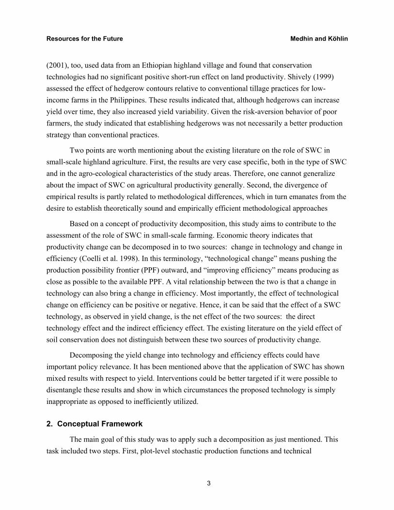
Resources for the Future Medhin and Koumlhlin
7
and identically distributed normal random variables with constant variance independent of Ui which is assumed to be non-negative exponential or half-normal or truncated (at zero) variables of N(μi σ2) where μi is defined by some inefficiency model (Coelli et al1998 Battese and Rao 2002) This arises from the nature of production andor cost functions The fact that these functions involve the concepts of minimality or maximality puts bound to the dependent variable To allow this most econometric frontiers assume one-sided inefficiency disturbances (Foslashrsund et al 1980)
Another important point here is the choice of the functional form of f () Battese (1992) noted that the translog or Cobb-Douglas production functions are the most commonly used functional forms for efficiency analysis The Cobb-Douglas specification was adopted for this study It is worth noting that each functional form has its own limitations most of which are related to the technical convenience of the functions and is not the result of deliberate empirical hypotheses In this case the robustness and the parametric linearity of the Cobb-Douglas function make it superior over other functional forms (Coelli 1995 Afriat 1972) The use of translog functions may also lead to excessive multicollinearity (Andre and Abbi 1996 Nyangena 2006)
For this application assume that there are j groups of firms in an industry classified according to their regional or organizational differences (or simply based on their ldquotechnologyrdquo) Suppose that for the stochastic frontier for a sample data of nj firms the jth group is defined by
( ) ( )ijij UVijij eXfY minus= β
jni 21= (5)
Assuming the production function is a Cobb-Douglas or translog form this can be re-written as
( ) ( ) ijijijijij UVXUVijij eeXfY minus+minus == ββ jni 21= (6)
3 One would argue that attributing rainfall and moisture differentials as error elements in a region known for its high dependence on rainfall and severe droughts excludes relevant variables It is a reasonable argument Unfortunately the data used in this study are not endowed with such variables However we firmly believe that as far as efficiency and productivity differentials are concerned this will have a limited impact on the results for two reasons First the data deal with areas of similar geo-climatic characteristics Second the study uses cross-sectional data Therefore it is more likely that rainfall and drought variations would affect efficiency and productivity evenly
Resources for the Future Medhin and Koumlhlin
8
We can soon see the advantage of such a representation Think now about the ldquooverallrdquo stochastic frontier of the firms in the industry without stratifying them into groups Such a frontier can be written as
( ) ( ) iiiii UVXUVii eeXfY minus+minus == ββ ni 21= sum= jnn (7)
Equation (7) is nothing but the stochastic metafrontier function The super-scripts differentiate the parameters and error terms of the metafrontier function from the group-level stochastic functions Note that Yi and Xi remain the same the only difference here is that separate samples of output and inputs of different groups are pooled into a single sample The metafrontier equation is considered to be an envelope function of the stochastic frontiers of the different groups This indicates that we can have two estimates of the TE of a firm with respect to the frontier of its group and with respect to the metafrontier
Mathematically iUi eTE minus= and
iUi eTE minus= respectively
The parameters of both the group frontiers and the metafrontier can be estimated using the method of maximum likelihood estimation After estimating β and β it is expected that the deterministic values Xijβ and Xiβ should satisfy the inequality Xijβ le Xiβ because Xiβ is from the metafrontier According to Battese and Rao (2002) this relationship can be written as
Xi
Xij
1 Ui
Ui
Vi
Vi
ee
ee
ee
minus
minus
sdotsdot= β
β
(8)
Equation (8) simply indicates that if there is a difference between the estimated parameters of a given group and the metafrontier it should arise from a difference in at least one of the three ratios namely the technology gap ratio (TGR) the random error ratio (RER) and the technical efficiency ratio (TER) That is
)(Xi
Xij
i
iUi
UiViVi
Vi
Vi
iXi
i TETE
eeTERande
eeRERe
eeTGR
iequiv=equiv=equiv= minus
minusminusminusminus ββ
β
β
(9)
The technology gap ratio indicates the technology gap for the given group according to currently available technology for firms in that group relative to the technology available in the who industry Note that this assumes all groups have potential access to the best available technology in the industry The TGR and the TER can be estimated for each individual firm
Note from our previous graphical presentation that 0 lt TEi le 1 and 0 lt TEi le 1 It also should be the case that TEi le TEi That is given that the frontier function of the group
Resources for the Future Medhin and Koumlhlin
9
containing firm i is enveloped by the metafrontier function the TE of firm i relative to the metafrontier is at least lower than that of relative to the group frontier Hence the TER is expected to be greater than or equal to unity
The random error ratio is not observable because it is based on the non-observable disturbance term Vi Therefore as far as estimation is concerned equation (8) can be rewritten as
iiUi
Ui
TERTGRee
ee
times=sdot= minus
minus
Xi
Xij
1 β
β
(10)
Combining (9) and (10) gives
ii TGRTETEi
times= (11)
Thus from equation (11) the TE relative to the metafrontier function is the product of the TE relative to the group frontier and the TGR of the technology group This is a very important identity in the sense that it enables us to estimate to what extent the efficiency (hence productivity) of a given firm or group of firms could be increased if it adopted the best available technology in the industry In our case we used this approach to estimate the technology gap between plots with and without soil conservation and investigate the role of different soil conservation practices in defining the technology of farm plots
23 Estimation of the Stochastic Metafrontier Curve
The metafrontier curve is an envelope of the stochastic frontier curves of the technology groups under discussion If each technology group has at least one firm which uses the best technology in the industry (ie if the TGR for the firm is 1) the metafrontier would be the curve connecting these best-practice firms from all groups In cases where no single firm of a given group qualifies for the best technology requirement the stochastic frontier of the group would lie below the metafrontier curve Stochastic frontiers for groups 2 and 4 in figure 2 are examples of this case
Resources for the Future Medhin and Koumlhlin
10
Figure 2 The Stochastic Metafrontier Curve
In reality all production points of the group stochastic frontiers may not lie on or below the metafrontier That is there could be outlier points to group stochastic frontiers (that is why they are stochastic) which could be also outliers to the metafrontier This indicates that estimating the metafrontier demands the very definition of the metafrontier as an assumption That is it assumes that all production points of all groups are enveloped by the metafrontier curve Therefore given the coefficients of group production functions output values and input values estimating the metafrontier is simply the search for the meta coefficients that result in a curve which best fits to the tangent points of the frontier group production functions with best technology firms
According to Battese et al (2004) for a Cobb-Douglas production function (or any function log-linear in parameters) β the metafrontier can be estimated using a simple optimization problem expressed as
Minimize Xrsquoβ
Subject to Xiβ le Xiβ (12)
In equation 12 Xrsquo is the row vector of means of all inputs for each technology group β is the vector group coefficients and β is the vector of meta coefficients we are looking for This is simply a linear programming problem Each plotrsquos production point will be an equation line in a sequence of simultaneous equation with an unknown right hand side variable Note that βs are
S frontier for Group1
S frontier for Group 2
S frontier for Group 4
The metafrontier curve Output Y
Inputs X
S frontier for Group 3
Resources for the Future Medhin and Koumlhlin
11
the maximum likelihood coefficients of the group stochastic frontier from our FRONTIER 414
estimations The constraint inequality is nothing but the envelope assumption we pointed out above
Once we obtain the solutions to out linear programming problem (βs) it is easy to calculate the TGRs and metafrontier technical efficiencies From equation (9) we know that
Xi
Xij
β
β
eeTGRi = and from equation (11) we have ii TGRTETE
itimes= Note that the TEi is already
estimated in our group stochastic frontiers
24 A Brief Empirical Review
A number of studies have investigated the TE of agriculture in various countries Helfand and Levine (2004) assessed the relationship between farm size and efficiency for Brazilian farmers using the data envelopment analysis and found that the relationship is more quadratic than the usual inverse linear relationship It also indicated that type of tenure access to institutions and modern input use have a significant relationship with efficiency differences Coelli and Battese (1996) used a stochastic frontier analysis for three villages in India Their results indicated that farm size age of household head and education are positively related with TE Battese at al (1996) found the same results for four agricultural districts of Pakistan On the other hand Bravo-Utreta and Evenson (1994) although they found significant levels of inefficiency for peasant farmers in Paraguay found no clear relationship of the high inefficiency with the determinants
Very few studies have assessed the relationship of soil conservation and efficiency In their TE analysis of potato farmers in Quebec Amara et al (1998) found that efficient farmers were most likely to invest in soil conservation Yoa and Liu (1998) assessed the TE of 30 Chinese provinces Their results showed that efficiency differentials were significantly related to the ldquodisaster indexrdquo which included physical characteristics such as soil water and infrastructure Irrigation was also found to have positive effect on TE
In the Ethiopian case Admassie and Heindhues (1996) found a positive relationship between TE and fertilizer use Seyum et al (1998) compared farmers within and outside the Sasakowa-Global 2000 project which primarily provided extension and technical assistance for
4 FRONTIER 41 is a software commonly used to estimate production frontiers and efficiency
Resources for the Future Medhin and Koumlhlin
12
farmers Their results showed that farmers participating in the project performed better Abrar (1998) pointed out that farm size age household size and off-farm income are the major determinants of TE in highland Ethiopia
To our knowledge no study has used the metafrontier approach to investigate agricultural efficiency in Ethiopia More importantly we have not found any other study that has used the metafrontier approach to assess the role soil conservation technologies in improving agricultural productivity
3 Data and Empirical Specification
The study is based on the Ethiopian Environmental Household Survey data collected by the departments of economics at Addis Ababa University and University of Gothenburg and managed by the Environmental Economics Policy Forum for Ethiopia (EEPFE) The survey covers six weredas
5 of two important highland zones in the Amhara Region in north Ethiopia Given the similarity of the socio-economic characteristics of the survey areas with other highland regions we believe that the results of the study can be used to comment on policies that aim to increase the productivity of highland small scale agriculture in Ethiopia
Due to the huge coverage of the data set in terms of crop type and land management activity the study focused on two major crop types (teff
6 and wheat) and three main soil conservation activities namely stone bund terracing soil bund terracing and bench terracing It should be noted that even though this data was dropped in the analysis part plots with other soil conservation types were also included in estimating the metafrontier efficiency estimates for the sake of methodological accuracy
The core motive for the need of the metafrontier approach to estimating efficiency is the expectation that plots under different soil conservation practices operate under different technologies If that is the case the traditional way of estimating efficiency by pooling all plots into the same data set may give biased estimates as plots with better technology will appear more efficient This indicates that one needs to test for the feasibility of the traditional approach before adopting the metafrontier That is we should test whether indeed plots under different
5 Wereda is the name for the second lowest administrative level in Ethiopia The lowest is kebele 6 Teff is a tiny grain used to make Ethiopiarsquos most common food item injera The grain has many variants based on its color
Resources for the Future Medhin and Koumlhlin
13
soil conservation practices have regularities in technical efficiency that make it useful to analyze them as different technologies In the meantime we will call them technology groups
As in former studies that applied the metafrontier approach this study uses the likelihood ratio test (LRT) To perform the LRT separate estimations should be performed for each technology group followed by an estimation of the pooled data
7
Teff and wheat crops were grouped according to the type of soil conservation applied in the 2002 main harvest season As can be seen from table 1 there are seven SWC technology groups The first four groups are the emphasis of this paper The stochastic frontier will have two major parts estimated simultaneously the production function and the technical effects While the first part estimates the coefficients of the farm inputs and the attached inefficiency the second part assesses the relationship between the estimated inefficiency and any expected determinants
This indicates that we have two sets of variables inputs and (efficiency) determinants Except for seed the inputs are described in table 1 for each group and for the pooled data The determinants include plot characteristics household characteristics market characteristics and social capital that are expected to affect the extent of TE Table 2 holds the details
Some input variables like fertilizer and manure have zero values for some plots As the model requires input and output values to be converted into logarithms dummy variables which detect such values were included in the production function This means the production function part of the model has two additional variables fertilizer dummy and manure dummy Hence 8 input and 23 determinant coefficients were estimated for each technology group While we identified the input coefficients as βi we identified the determinant coefficients as δi
7 The test compares the values of the likelihood functions of the sum of the separate group estimations and the pooled data In a simple expression the value of the likelihood-ratio test statistic (λ) equals -2ln[L(H0)] - ln[L(H1)] where ln[L(H0)] is the value of the log-likelihood function for the stochastic frontier estimated by pooling the data for all groups and ln[L(H1)] is the sum of the values of the log likelihood functions of the separate groups (Greene 2003)
Environment for Development Medhin and Koumlhlin
14
Table 1 SWC technology Groups
Technology Group Variable Min Max Mean Std
dev Var Technology Group Variable Min Max Mean Std
dev Var
Yield(kgha) 688 1097293 103587 98143 96321166 Yield(kgha) 1324 1726384 125140 120168 1444035
Labor(days) 190 28400 3861 3010 90620 Labor(days) 600 20800 4516 2707 7331
Traction(days) 25 6000 574 577 3337 Traction(days) 100 3600 756 433 18804
Fertilizer(ETB) 00 54900 2499 7726 597056 Fertilizer(ETB) 00 92200 4319 12055 145332
None
(667 plots)
Manure(kg) 00 620000 4179 30540 9327222
Contour furrowing
(473 plots)
Manure(kg) 00 805005 4337 41247 170132
Yield(kgha) 6018 809160 95576 92267 85132708 Yield(kgha) 20415 527798 143205 91721 841267
Labor(days) 350 31700 4897 4186 175293 Labor(days) 1300 10900 4421 2172 47173
Traction(days) 25 2600 479 409 1676 Traction(days) 100 4500 811 462 2131
Fertilizer(ETB) 00 48850 2066 6382 407389 Fertilizer(ETB) 00 50100 6544 14232 202552
Stone bunds
(357 plots)
Manure(kg) 00 93000 5803 15255 2327220
Contour plowing
(97 plots)
Manure(kg) 00 214668 5186 26964 727034
Yield(kgha) 6018 474422 81532 66799 4462131 Yield(kgha) 3833 299154 97934 63159 398906
Labor(days) 750 25900 3980 3742 140054 Labor(days) 850 24900 4563 4086 16691
Traction(days) 50 3600 523 461 2127 Traction(days) 100 1900 484 343 1176
Fertilizer(ETB) 00 25100 1416 4885 238694 Fertilizer(ETB) 00 50100 2716 8530 72766
Soil bunds
(98 plots)
Manure(kg) 00 68934 3726 12440 1547751
Others
(85 plots)
Manure(kg) 00 1760010 28189 191180 3654970
Yield(kgha) 994 397472 94379 63597 40446414 Yield(kgha) 688 1726384 107602 99643 992862
Labor(days) 700 21000 4796 3501 122585 Labor(days) 190 31700 4342 3303 10921
Traction(days) 50 5700 699 695 4832 Traction(days) 25 6000 615 514 2637
Fertilizer(ETB) 00 28000 2874 6963 484894 Fertilizer(ETB) 00 92200 3057 9180 84270
Manure(kg) 00 243335 6496 27313 7460520 Manure(kg) 00 1760010 5770 50430 254318
Bench terraces
(106 plots)
Notes Std dev = standard deviation ha = hectare ETB = Ethiopian birr US$ 1 = ETB 85 Oxen days
Pooled
(1883 plots)
Notes Std dev = standard deviation ha = hectare ETB = Ethiopian birr US$= ETB 85 Oxen days
Resources for the Future Medhin and Koumlhlin
15
Table 2 Definition of Variables
Part 1 Production function
Part 2 Technical effects function
Plot output and inputs Plot characteristics Household characteristics Social capital
LnOutput natural logarithm of kg output
plotage plot age (years that the household cultivated the plot)
Malehh dummy for sex of household head (1 if male 0 if female)
deboD dummy for Debo participation (1 if yes 0 if no)
LnLand natural logarithm of hectare plot area
plotdishome distance from home (minutes of walking)
Agehh age of household head in years
trust number of people the household trusts
LnLabor natural logarithm of labor (person days)
hireD hired labor use dummy (1 if used 0 otherwise)
Educhh years of schooling attended by household head
assi-inD dummy for any assistance received from neighbors (1 if yes 0 if no)
LnTraction natural logarithm of animal traction (oxen days)
Plot Slope meda as a base case Hhsize total family size of the household
assi-outD dummy for any assistance forwarded to neighbors (1 if yes 0 if no)
LnSeed natural logarithm kg seed
dagetD dummy for daget (1 if daget 0 otherwise)
mainacthh dummy for main activity of the household head (1 if farming 0 otherwise)
LnFert natural logarithm of fertilizer applied (ETB)
hillyD dummy for hilly (1 if hilly 0 otherwise)
Offarm total income earned off farm throughout the year
LnMan natural logarithm of manure (kg)
gedelD dummy for gedel (1 if gedel 0 otherwise)
Liv-value total value of livestock owned by the household
fertD dummy for fertilizer use (1 if used 0 otherwise)
LemD dummy for soil quality (1 if lem 0 otherwise)
Farmsize total farm size cultivated by the household in hectares
ManD dummy for manure use (1 if used 0 otherwise)
Cultivation arrangement own cultivation as a base case
Distownm distance to the nearest town in walking minutes
sharecD dummy for share cropping (1 if share cropped 0 otherwise)
rentD dummy for rented plot (1 if rented 0 otherwise)
irrigD irrigation dummy (1 if irrigated 0 otherwise)
Environment for Development Medhin and Koumlhlin
16
The mathematical expressions of the two parts of the stochastic frontier to be estimated are
(the production function)
)exp(
lnlnlnlnlnlnln
ijijijojijoj
ijojijojijojijojijojijojij
UVmanDFertD
manfertseedtractionlaborlandOutput
minus+++
+++++=
ββ
ββββββ
(13)
and the technical effects function (where μi is the mean level of technical inefficiency8 for plot i
in technology group j calculated from (13)
ijijjijjijjijjijj
ijjijjijjijjijjijj
ijjijjijjijjijjijj
ijjijjijjijjijjijjojij
eplotsidhiredDhillyDgedelDdagetD
lemDirrigDrentDsharecDplotageinDassi
outDassitrustdeboDdistownfarmsizevalueliv
offarmmainactDhhsizeeduchhagehhmalehh
ωδδδδδ
δδδδδδ
δδδδδδ
δδδδδδδμ
++++++
+++++minus+
minus+++++minus+
++++++=
hom2322212019
181716151413
121110987
654321
(14)
(wij is a random error term)
For each technology group equations (13) and (14) are (simultaneously) estimated using FRONTIER 41 In addition to the β and δ coefficients the TE of each plot and the log-likelihood functions are also estimated The pooled data are also estimated in the same manner The pooled estimation is critical to the formation of the metafrontier as one should perform the log likelihood test described above
If the LRT gives a green light for use the metafrontier the next step is estimating the stochastic metafrontier function This is done in accordance with the approach discussed in the second chapter Note that in our model we have 8 inputs 7 groups and 1883 plots
The Mathematica 51 software was used to solve the linear programming problem and estimate the meta coefficients Once we estimated the meta coefficients it was easy to calculate the TGR and metafrontier efficiency of each plot in each technology group Besides getting more precise estimates of TE a major emphasis of this study was to assess the extent of the technology-based productivity differential especially between the first four soil conservation groups in table 3 if any It should be noted that the fact that the LRT signals for the use the
8 μi is discussed in appendix 1 together with the maximum likelihood estimation of TE
Resources for the Future Medhin and Koumlhlin
17
metafrontier approach does not guarantee that some groups have better technology than others That is even if the test indicates plots with different soil conservation technologies cannot be pooled into the same frontier model it does not necessarily guarantee that some conservation technologies have better productivity than others Neither does it guarantee that technology gaps if any are only because of soil conservation as plot technology also constitutes many other factors some related to soil conservation adoption
4 Discussion of Results
Productivity change is caused by efficiency andor technology change If the production process of farm plots involves technical inefficiency this means that there is room for improving productivity at the presently available technology at least in the short run But an important point in the technology-efficiency paradigm of productivity change is that technology change may affect the level of efficiency either positively or negatively Therefore a careful analysis of any effect of technology on efficiency is important as it may give a clue to why some technologies that are efficient in controlled environments fail and why others happen to be surprisingly effective when they are applied in the real world The hypothesis is that the hidden change in efficiency because of the technological change may be the reason In this section our main emphasis is looking into the relationship of SWC and the determinants of TE
41 Technical Efficiency and Soil Conservation Group Stochastic Frontiers
Table 3 summarizes the maximum likelihood coefficient estimates of the stochastic production for the different technology groups including the pooled data Most of the estimates are positive and significantly different from zero Note that the parameter estimates of the pooled data are still relevant for the production function even if the LRT rejects the pooled representation That is technological variability within the pooled representation will only bias the TE estimates not the production function coefficient estimates
Plots cultivated under all SWC technologies experience a considerable level of technical inefficiency An important point is that plots without any SWC technology are the least efficient ones with a TE of 0654 At this stage we cannot conclude that plots with SWC have higher productivity than plots without SWC because they have higher TE Such comparison is valid only if we are sure that the two groups operate at similar technology or if the pooled
Resources for the Future Medhin and Koumlhlin
18
Table 3 Coefficients of the Production Function (βs)
Coefficient (t-ratio)
Variable None Soil bunds Stone bunds Bench terraces Pooled
β0
Land
Labor
Traction
Seed
Fertilizer
Manure
Fertilizer use dummy
Manure use
dummy
42487 (204663)
03496 (80103)
02794 (59290)
02081 (53726)
02502 (103058)
-00878
(-15757)
00613 (11711)
04230
(16245)
-02959 (-11053)
43130 (47752)
03436 (16600)
02992
(16263)
-01521 (-11041)
02678 (28847)
-01332
(-06145)
01215 (06437)
05533
(05705)
-03893 (-03986)
45430 (147057)
02377 (43778)
01408 (25056)
03395 (60643)
01193 (31099)
-00248
(-01993)
01541 (23833)
00575
(00973)
-06386 (-18279)
58685 (63162)
07310 (38998)
00082
(004735)
03116 (24046)
00866
(12983)
00381 (03887)
-01461
(-10644)
-00605 (-01352)
11504
(14711)
43618 (354124)
03149 (120299)
02290 (84113)
02071 (82998)
02337 (155857)
-00038 (01303)
00235
(08208)
00410 (02832)
00116
(00758)
Note significant at α=005 significant at α=010
representation is valid The value of the LRT statistic (λ) was calculated to be 37124 The Chi-square test at 8 degrees of freedom
9 shows that this is significant at α = 0005
10 That is the null
hypothesis that says the pooled stochastic estimation is a correct representation of the data is
9 The number of restrictions is 8 10 χ2
8 (0005) = 21 9550 lt 37124 the null hypothesis is rejected
Resources for the Future Medhin and Koumlhlin
19
rejected Most importantly it means that there is a significant technology differential among the four groups in tables 3 and 4
Table 4 Mean TE and the Coefficients of the Technical Effects Function
Variable None Soil bunds Stone bunds Bench Pooled
Mean TE 065498 077971 067615 068731 067825
δ0 -68962 (-26735)
10558 (01076)
-26569 (-20452)
-43708 (-04472)
-96613 (-43111)
Sex (dummy) 12182 (17476)
-68500 (-08454)
37077 (27549)
12617 (01090)
19818 (37108)
Age 04960 (29383)
-00433 (-03123)
02702 (23600)
04447 (22635)
06415 (48117)
Education -01404 (-04175)
-03246 (-04170)
-01417 (-03791)
-11810 (-10822)
-03474 (-18520)
Household size 02045 (05005)
-00578 (-00520)
-01968 (-03112)
25167 (16728)
07351 (27342)
Main activity -10623 (-17635)
21261 (02891)
-19442 (-25224)
-107105 (-10941
-94019 (-29118)
Off-farm income -00079 (-18921)
-00007 (-03056)
00060 (18899)
-00134 (-14099)
-00064 (-33254)
Livestock value -00059 (-29657)
-00030 (-12549)
-00009 (-08834)
-00034 (-18948)
-00077 (-51426)
Total farm size 21393 (18683)
12783 (040663)
-02277 (-11995)
10189 (30714)
2992 (36047)
Distance to town 00788 (27139)
00312 (04933)
00023 (09623)
-00263 (-04255)
00578 (39907)
Debo participationDagger 82177 (25904)
32114 (06406)
-12368 (-20270)
-17534 (-16866)
69117 (30831)
Trust 29064 (27174)
30401 (12716)
01730 (14437)
-64733 (-24664)
37709 (45653)
Assistance out 08798 (02607)
10665 (01862)
-01818 (-02995)
24201 (02505)
28926 (14989)
Assistance in 54461 (16355)
16024 (02104)
-43070 (-08385)
124097 (15060)
14449 (46344)
Plot age 00060 (0583)
-00979 (-04386)
-00145 (-071709
-1211 (-37327)
-02968 (-34008)
Sharecropping 9664 (25071)
-46274 (-04832)
-06560 (-10204)
-23074 (-23585)
-32866 (-13362)
Resources for the Future Medhin and Koumlhlin
20
Variable None Soil bunds Stone bunds Bench Pooled
Rented plot 27494 (23689)
-10917 (-10949)
-157011 (-13543)
00000 (00000)
117834 (12167)
Irrigated plot -177503 (-15543)
00000 (0000)
45381 (04590)
-66149 (-05901)
-37566 (-03838)
Soil quality (lem) 11298 (29373)
15768 (04681)
29235 (12979)
-11431 (-18835)
13511 (13065)
Slope 1 daget 30071 (08710)
-24226 (-07463)
-40035 (-13371)
-58438 (-10081)
-3894 (-27111)
Slope 2 gedel -63602 (-22769)
-99969 (-11439)
41842 (04611)
61680 (06356)
-10658 (-23365)
Slope 3 hilly -58643 (-18064)
11059 (01106)
14767 (25999)
00000 (00000)
376805 (42053)
Hired labor -8983 (-17960)
49991 (05541)
-14379 (-19570)
-87772 (-11541)
-15919 (-41300)
Plot distance to home
0066 (16809)
00162 (01325)
00915 (11901)
01137 (06470)
00594 (24021)
Sigma 2 20749 (39425)
2720 (29200)
8152 (53933)
59377 (36084)
28803 (59753)
Gamma 8977
(358897) 19297
(06559) 7453
(112089) 77165 (90520)
9260 (891217)
Notes significant at α=005 significant at α=010 Dagger See text footnote 13 for explanation of Debo project
Before going to the details it is important to clarify what the TE-determinant estimates in table 4 mean and what they do not mean in the presence of the technology differential First the estimates of the pooled specification in the last column are not valid any more Second any TE-based productivity comparison among the four groups should take into account that they operate at different technologies That is the fact that a given group has higher TE does not mean it is more productive it means plots under this group operate closer to their group technology frontier which is not necessarily the best technology frontier compared to frontiers of other groups Therefore productivity comparisons are only possible only if we know the position of group frontiers relative to the best technology frontier in all groups or the metafrontier Third the fact that the LRT rejects the pooled representation of the data does not invalidate the group-level TE and inefficiency-determinant coefficient estimates It only limits their universality across technology groups group technical inefficiency for plot i in technology group j is the
Resources for the Future Medhin and Koumlhlin
21
potential improvement in output if plot i applies the best technology available in group j This will be clear when we look into our results from the stochastic metafrontier estimation
In addition to technology differentials it is also appropriate to deal with non-random forces that could affect output The user cost of SWC is one such variable Even though our data failed to give a precise estimate some studies have shown that SWC investment takes away a considerable amount of land and labor from the production process (Shiferaw and Holden 1998 2001) In our case the land cost is important because the plot size in our production functions does not account for the land lost to SWC While the labor input in our production function does not include the amount of labor spent on constructing or maintaining SWC structures
11 the land
lost is included in the plot size as if it was used for crop cultivation Hence every unit of output lost for every unit of land occupied by SWC structures is detected as if it resulted from technical inefficiency This indicates that TE estimates for plots with SWC could be understated by our model which stresses our point that conserved plots are more efficient that unconserved ones Such downward effect is more interesting if the land cost varies with plot characteristics as will soon be shown
Some plot characteristics in the technical-effects model could be related to SWC adoption In such cases the results for each technology group should be interpreted by taking into consideration the adoption effect If for example the probability of a plot being conserved increases with the plot having an attribute i and ifmdashfor a given SWC technologymdashefficiency is positively related with attribute i it is logical to suspect that it is the presence of attribute imdashnot soil conservationmdashthat is the reason for better efficiency On the other hand if we have no evidence that the probability of soil conservation is related to the plot having attribute i and if efficiency is positively related to attribute i for conserved plots and negatively related (or not related at all) for unconserved plots we can conclude that SWC positively affects efficiency through attribute i However it should be noted that our results may not be as simple as these clean cases This is mainly because efficiency may have various determinants which could have different effects for each conservation technology
12
11 The labor cost of SWC does not affect the TE estimate even though it could affect allocative efficiency (AE) estimates 12 This indicates that SWC could also be related to AE Although the analysis of AE is far from the scope of this study we believe that it would have helped in understanding the complex relationship between soil conservation and productivity Among other things this requires good price data
Resources for the Future Medhin and Koumlhlin
22
It is assumed that farmers tend to conserve highly degraded plots relative to less degraded plots In the absence of detailed soil composition data plot slope and soil quality are the best proxies for soil degradation That is if highly degraded plots have a better chance of being conserved the probability of SWC could also increase with steep slope and poorer soil quality Table 5 shows the results of the Mann-Whitney test
Table 5 Mann-Whitney Test for Plot Slope and Soil Quality
Plot characteristics Hypotheses Z-value P-value
Slope H0 SlopeC = SlopeU
H1 SlopeC gt SlopeU 66104 0000
Soil quality H0 Soil QC = Soil QU
H1 Soil QC lt Soil QU 14220 00778
Notes C= conserved U = unconserved significant at α = 001 significant at α = 01
The null hypothesis that conserved plots and unconserved plots have similar slopes is rejected at a very high level of significance That is steeper plots have a higher likelihood of being conserved in the study areas As for soil quality the null hypothesis that plots with poorer soil quality get more attention in the conservation decision is not rejected unless we are willing to accept a 778-percent room for error The moderate decrease in soil quality with soil conservation could be because of the negative correlation between slope and soil quality (with partial correlation of 0158) In other words conservation decision may be based on expected vulnerability to soil erosion rather on increasing soil quality More specifically farmers may choose to conserve better soil-quality plots on steep slopes rather than low quality plots on moderate slopes This is certainly worth investigating in further research as it could be related to the risk aversion of poor farmers invest to protect what you already have rather than upgrade what is lost
We now have evidence that plot slope is related to the conservation decision This indicates that any relationship between slope and efficiency should be assessed critically taking into consideration that conserved plots have steeper slopes From table 4 steep slope is negatively related to technical inefficiency for plots without SWC On the other hand steep slope is positively related to technical inefficiency for plots with stone bunds while there is no significant relationship for the other SWC technologies That is unconserved steep plots have better TE than conserved steep plots An explanation for this could be the relationship between the per-hectare land cost of SWC with plot slope Shiferaw and Holden (2001) estimated that for
Resources for the Future Medhin and Koumlhlin
23
a 45-percent increase in slope the per-hectare land lost for SWC increases by 900 percent The fact that the negative impact of such high land costs on output is now absorbed as technical inefficiency justifies the result that the positive relationship of high slope and TE disappears with the introduction of SWC
High soil quality and TE are negatively related for unconserved plots and positively related for plots with bench terraces Furthermore there is no significant relationship for plots with stone bunds and soil bunds That is soil conservation erases or alters the negative relationship of high soil quality and TE This means even though high soil-quality plots have a slightly lower likelihood of being conserved they have higher TE than unconserved high soil-quality plots other things held constant
The relationship between the gender of household heads and TE is surprising The fact that a household is headed by a male is negatively related to TE for unconserved plots and for plots with stone bunds the relationship being stronger in the latter group This is contrary to many studies which showed female-headed households are less efficient than male-headed households Age of household head is also negatively related to efficiency except for plots with soil bunds where there is no significant relationship Education has a non-significant positive relationship with TE for all technology groups Unconserved and stone bund plots cultivated by household heads with farming as a main activity have higher TE The positive relationship is more pronounced in the case of stone bunds Off-farm income has a weak positive relationship with efficiency for plots without soil conservation and a rather weaker negative relationship for stone bund plots Increasing livestock wealth has a small but positive effect on efficiency although it is insignificant for stone and soil bunds Larger total farm size has a negative relationship with efficiency at least for unconserved plots and plots with bench terraces
Plot distance from home has a negative effect on TE for plots without conservation while it has no significant effect for plots with SWC The same is true for distance to the nearest town Sharecropping is negatively related to efficiency for unconserved plots while it has a strong positive relationship for plots with bench terraces Land rental is also negatively related to efficiency for plots without conservation while it has a non-significant relationship for conserved plots Plots which employed hired labor have better efficiency especially if they have stone bund structures
Resources for the Future Medhin and Koumlhlin
24
Unconserved plots cultivated by households who participate in Debo13 have lower efficiency while Debo participation is positively related to efficiency for plots with stone bunds and bench terraces It has no significant relationship for plots with soil bunds Unconserved plots cultivated by peasants who trust more people in their neighborhood are also less efficient than conserved plots That is soil conservation alters the negative relationship of higher social capital and efficiency
The above paragraphs indicate that in most cases negative relationships between various plot and household attributes and TE disappear or are reversed in the presence of one of the soil conservation technologies That is for some reason soil conservation positively affects the role of the determinants of efficiency Studying the explicit aspect in which soil conservation affects the role of plot household market characteristics and social capital in determining the level of TE could shed new lights on the economics of soil conservation adoption and productivity analysis This is certainly an attractive area of further research
It is important to note that the fact that conserved plots have higher TE does not necessarily mean they also have higher yield than plots without soil conservation It simply means that the chosen amounts of inputs were used more effectively in the case of conserved plots Table 6 below compares the yield and input values of plots with and without soil conservation The average yield for plots with conservation is significantly lower than that of plots without conservation even though the difference is not significant Conserved plots use a significantly higher amount of labor than unconserved plots while the latter use a higher amount of seed The differences in manure fertilizer and traction are insignificant
As can be seen in table 6 even though conserved plots have higher TE than unconserved plots they still have lower mean yield One reason for this is the fact that conservation decision is partly based on plot characteristics such as plot slope and soil quality that have a significant impact on yield in their own right Therefore direct yield and input comparisons can only be used to comment on the effect of productivity technologies if plots are homogenous or if the
13 Debo is a non-profit organization focused on helping alleviate extreme poverty in rural Ethiopia It offers a wide range of projects (education agriculture health water development and reforestation plus microcredit and job skills training) implemented with a local non-profit partner Debo Yeerdata Mahiber The agricultural projects work with rural communities ldquoto boost food production promote sustainable environment and overcome povertyrdquo primarily through reforestation to reclaim soil erosion and creation of local nurseries to supply trees See httpdeboethiopiaorgsourceProgramsDeboProgramshtml
Resources for the Future Medhin and Koumlhlin
25
conservation decision is independent of plot characteristics that affect output One point that should be kept in mind is that SWC could be productivity enhancing even if it does not lead to the highest yield simply because it is not the only determinant of yield The discussion of the metafrontier results in the next section elaborates this point
Table 6 Yield and Input Use Comparison
Variable With soil conservation Without soil conservation Difference
Mean Std dev Mean Std dev With-without P-value
Yield (kgh) 92897 83491 103587 98143 -10690 0 0421
Labor (days) 4718 3998 3862 3010 856 00002
Manure (kg) 5571 17761 4180 30540 1391 03309
Fertilizer (ETB) 2105 6271 2499 7727 -394 03594
Traction (oxen days)
528 491 574 578 -046 01391
Seed (kg) 1805 4074 2619 4018 -814 00000
Std dev = standard deviation ETB = Ethiopian birr US$ 1 = ETB 85
42 Technical Efficiency and Technology Gaps Metafrontier Estimation
Table 7 illustrates the results of the metafrontier estimation in combination with the group TE results from table 4 Note that while group technical inefficiency (1 - group TE) for plot i in technology group j is the potential improvement in output if plot i applies the best technology available in group j On the other hand metafrontier technical inefficiency for plot i in technology group j is the potential increase in output if plot i applies the best technology available in all groups The mean TGR for a given group quantifies the average gap between group technology and overall technology The maximum value 1000 indicates that at least one plot in the group uses the best technology available for all groups In other words group frontiers with maximum TGR of 1000 are tangential to the metafrontier curve All group frontiers are tangential to the metafrontier except for bench terraces
Plots with soil bunds have the lowest mean TGR 07806 This simply indicates that even if all soil bund plots attain the maximum technology available for the group they will still be about 219 percent away from the output that they could produce if they used the maximum
Resources for the Future Medhin and Koumlhlin
26
Table 7 Technology Gaps and Metafrontier TE
Technology group Variable Minimum Maximum Mean Std dev
None TGRa
Meta TE Group TE
06134 01133 01133
10000 098682 098687
09494 062061 065497
009972 017301 016892
Stone bunds TGR Meta TE Group TE
06558 012449 014898
10000 093073 093080
09539 064607 067614
008123 018027 017716
Soil bunds TGR Meta TE Group TE
05264 015034 017841
10000 092095 097442
07806 060600 077970
008881 015727 019122
Bench terraces
TGR Meta TE Group TE
05499 013687 013688
09999 094353 094464
09629 065748 068733
008881 020040 020766
TGR= technology gap ratio Std dev = standard deviation
technology available in the whole sample The significantly lower value of the meta TE relative to the all higher group TE says exactly the same Although the potential improvement in output relative to the best technology available for soil bund plots is only 2203 percent it is 394-percent relative to the best technology available for all groups Note that meta TE is not a real efficiency measure per se It only quantifies by how much output could be increased if a given group had the best technology We can say a plot is technically inefficient only if it fails to produce the maximum attainable output using the technology it applies
Now it is time to face the big question is SWC a good technology
From table 7 we see that plots without SWC have no significant technology gap relative to plots with three SWC technologies Moreover it is plots with soil bunds which have the highest technology gap (lowest TGR) From these results it seems logical to conclude that plots with SWC do not use higher technology than plots without soil conservation This may seem a short answer to the big question but it is not Actually it is not an answer to the question at all Our question is not whether plots with SWC have better technology it is whether SWC is a good
Resources for the Future Medhin and Koumlhlin
27
technology Given that a given plotrsquos technology constitutes other factors14
in addition to soil conservation it could be the case that plots without SWC have a better composite technology than plots with soil conservationmdashso soil conservation could still be a good technology
Note that this point is strictly related to our earlier finding that soil conservation adoption is dependent on plot characteristics
15 This means adoption of a given type of SWC technology is
related to a plotrsquos prior composite technology More specifically SWC technology has been shown to be adopted in plots with poor conditions In such cases it is possible that SWC improved the composite technology of conserved plots and that still unconserved plots have a higher composite technology Accordingly we can say that a given type of SWC is a better technology if among others one of the following is satisfied First a given SWC technology is good if conserved plots could have performed worse had they not been conserved Second soil conservation is a good technology if unconserved plots could have performed better had they been conserved
One way to assess these requirements is to start by answering the question of which plots have the best technology These are the plots with a TGR very close to the value 1000 from our metafrontier estimation Studying the technology characteristics of these frontier plots in some detail could shed some light on the role of soil conservation Table 8 is a summary of descriptive values and frequencies of plot characteristics that define the metafrontier technology We have now identified the 147 plots that define the best practice in the 1228 plots that were cultivated under the four technology groups including plots without conservation (which are 543 percent of the sample) Our goal was to look for the role of plot characteristics
16 in making the frontier in
all conservation types That is we were looking for the remaining variables that defined the composite technology besides soil conservation
17
14 Plot characteristics farming equipment and farmer ability are also primary components of the composite technology If plots and their farmers were homogenous we could argue that the difference in technology is only because of soil conservation 15 Plot characteristics could include plot slope and soil quality For simplicity we can identify them as natural technologies 16 Usage of modern inputs such as fertilizer also affects the composite technology But in table 6 we found that there is no significant difference in the use of such inputs between conserved and unconserved plots 17 If we had plot-level moisture data table 8 could have been more informative as moisture level would certainly affect the technology position of plots
Resources for the Future Medhin and Koumlhlin
28
Table 8 Characteristics of Best Technology Plots
Soil conservation technology ( share)
Plot characteristics None Stone bunds
Soil bunds
Bench terraces All best
share in whole sample
Plot slope
Meda Dagetma Gedel Hilly
773 227
0 0
679 250 71 0
250 500 250
0
833 83 83 0
728 231 41 0
700 267 24 07
Soil quality
Lem Lem-tef Tef Other Chora
413 307 280 00 00
482 375 143 00 00
250 500 250 00 00
250 750 00 00 00
422 374 204 00 00
401 416 180 01 01
Soil type
Black Red Brown Gray Black red
240 693 13 13 27
464 500 00 18 18
0 1000 00 00 00
833 167 00 00 00
367 585 7 14 20
420 511 2 19 29
Crop type
White teff Mixed teff Blackred teff Wheat
147 147 187 520
196 18
143 643
500 00
250 250
500 83
167 250
204 88
170 537
298 121 243 338
Number of frontier plots 75 56 4 12 147
Total number of plots 667 357 98 106 1228
Percentage of frontier plots
112 156 40 113 119
The roles of plot slope soil quality soil type and crop type were examined Of the plots which define the best practice 728 percent have a plain slope (meda) and 394 percent have no soil conservation technology It is worth noting that the share of steep plots in the best-practice group increases with SWC technology This could be again related to the fact that steep plots have a higher likelihood of being conserved This finding asserts our earlier proposition that the positive relationship between plot slope and technical inefficiency emanates from the increase of land costs of SWC with slope In all conservation types good soil-quality plots also have a better share in the best technology group
Corrected to its sample share the stone bunds group has the highest number of plots that qualify as best practice (156 percent) Bench terraces none and soil bunds follow with shares of
Resources for the Future Medhin and Koumlhlin
29
113 percent 112 percent and 40 percent respectively This indicates that even though the ldquono SWCrdquo group has the highest share of plots in the sample space soil conservation groups outrank it in the best plots scenario except for soil bunds In general the shares of different plot-characteristics categories in the best-practice group are closely related to their shares in the sample space An important lesson from table 8 is that plots with a better soil and topographic condition (advantaged plots) with or without SWC still define the best technology in the survey areas SWC helps by giving this chance to disadvantaged plots Therefore soil conservation is a good technology
The metafrontier approach also gives new insights into the group-level TE estimates The best example in our case is the soil bunds group Although plots cultivated with soil bunds have a relatively lower technology their high mean group TE indicates their lower technology is used more efficiently than plots cultivated with other soil conservation practices If in some way their high efficiency is related to their soil bund terraces we cannot conclude that soil bund terracing is a bad technology as there could be a net productivity improvement Output of plots with soil bunds could be increased by 4 percent if they were conserved with stone bunds because of better technology On the other hand the output of plots with stone bunds could be increased by 104 percent if they were conserved by soil bunds because of higher efficiency Therefore the output of plots with stone bunds could be increased by 64 percent if they were conserved by soil bunds because what matters is the net effect of technology and efficiency Soil bund terracing is an even better technology
5 Concluding Remarks
This study used the newly developed metafrontier approach to assess the TE of small-scale food production in the Ethiopian highlands at plot level with the main goal of investigating the role of soil conservation technology in enhancing agricultural productivity To this end stochastic frontiers were estimated for four technology groups including a group of plots without soil conservation technology After testing for technological difference among groups a metafrontier production curve was estimated and technology gaps of each plot in each technology group were calculated
The group stochastic frontier estimations showed that plots with SWC technologies are relatively more efficient than plots without soil conservation For all soil-conservation technology groups mean technical inefficiency was regressed against various plot household market and social capital variables The results indicated that the likelihood of negative technical effects decreased with SWC Most importantly these results showed that that the
Resources for the Future Medhin and Koumlhlin
30
decomposition of the yield productivity effect of farm technologies into technology and efficiency effects has indeed relevant policy values Studying the aspects in which a given SWC affects efficiency could shed some light on why laboratory-effective SWC technologies underperform in the real world
The stochastic metafrontier estimation showed that plots cultivated under different SWC practices operated under different technologies This indicated that efficiency estimations that fail to take into account such technology differential could lead to biased results An in-depth look at the characteristics of best-practice plots showed that SWC is a major part the definition of a plotrsquos composite technology but not all of it While advantaged plots dominated the frontier regardless of their conservation status disadvantaged plots made it to the frontier with the help of SWC Hence SWC proved to be good technology
The stochastic metafrontier proved to be promising in the quest for a methodology that enables us to assess the productivity effect of new technologies or policy interventions in industries with heterogeneous firms and production strategies In small-scale agriculture the prevalence of such heterogeneities is usually the biggest challenge in the design of policies and strategies to boost productivity For example a critical issue in the economics of SWC in small-scale agriculture is the matching problem which SWC practice fits which agro-economic environment One can approach this problem by performing a metafrontier estimation on plots under different agro-economic environments and identifying which SWC works better with which plothousehold attributes
Resources for the Future Medhin and Koumlhlin
31
References
Abrar S 1998 ldquoIdentifying the Sources of Technical Inefficiency of Ethiopian Farmers Using the (Single Stage) Stochastic Frontier Inefficiency Modelrdquo Working Papers series Addis Ababa Ethiopia Addis Ababa University Department of Economics
Admassie A and F Heindhues 1996 ldquoEstimation of Technical Efficiency of Smallholder Farmers in the Central Highlands of Ethiopiardquo Ethiopian Journal of Agricultural Economics 1(1) 19ndash35
Afriat SN 1972 ldquoEfficiency Estimation of Production Functionsrdquo International Economic Review 13(3) 568ndash95
Aigner DJ CAK Lovell and P Schmidt 1977 ldquoFormulation and Estimation of Stochastic Frontier Production Function Modelsrdquo Journal of Econometrics 6 21ndash37
Alemu T 1999 ldquoLand Tenure and Soil Conservation Evidence from Ethiopiardquo PhD diss (92) School of Economics and Commercial Law University of Gothenburg Sweden
Amara N N Traoreacute R Landry and R Romain 1998 ldquoTechnical Efficiency and Farmersrsquo Attitudes toward Technological Innovation The Case of the Potato Farmers in Quebecrdquo Canadian Journal of Agricultural Economics 47(1) 31ndash43
Croppenstedt A and A Mammo 1996 ldquoAn Analysis of the Extent of Technical Efficiency of Farmers Growing Cereals in Ethiopia Evidence from Three Regionsrdquo Ethiopian Journal of Economics 5(1) 39ndash62
Battese G E 1992 ldquoFrontier Production Functions and Technical Efficiency A Survey of Empirical Applications in Agricultural Economicsrdquo Agricultural Economics 7 185ndash208
Battese GE and TJ Coelli 1988 ldquoPrediction of Firm-Level Technical Efficiencies with Generalized Frontier Production Function and Panel Datardquo Journal of Econometrics 38 387ndash99
Battese GE SJ Malik and MA Gill 1996 ldquoAn Investigation of Technical Inefficiencies of Production of Wheat Farmers in Four Districts of Pakistanrdquo Journal of Agricultural Economics 47 37ndash49
Battese GE and DSP Rao 2002 ldquoTechnology Gap Efficiency and a Stochastic Metafrontier Functionrdquo International Journal of Business and Economics 1(2) 1ndash7
Resources for the Future Medhin and Koumlhlin
32
Battese GE DSP Rao and CJ OrsquoDonnell 2004 ldquoA Metafrontier Production Function for Estimation of Technical Efficiencies and Technology Gaps for Firms Operating under Different Technologiesrdquo Journal of Productivity Analysis 21 91ndash103
Bravo-Ureta BE and RE Evenson 1994 ldquoEfficiency in Agricultural Production The Case of Peasant Farmers in Eastern Paraguayrdquo Agricultural Economics 10 27ndash37
Byiringiro F and T Reardon 1996 ldquoFarm Productivity in Rwanda Effects of Farm Size Erosion and Soil Conservation Investmentrdquo Agricultural Economics 15 127ndash36
Coelli T 1995 ldquoRecent Developments in Frontier Modeling and Efficiency Measurementrdquo Australian Journal of Agricultural Economics 39(3) 219ndash45
Coelli T and GE Battese 1996 ldquoIdentification of the Factors Which Influence the Technical Inefficiency of Indian Farmersrdquo Australian Journal of Agricultural Economics 40(2) 103ndash28
Coelli T DSP Rao C OrsquoDonnell and GE Battese 1998 An Introduction to Productivity and Efficiency and Productivity Analysis 2nd ed New York Springer
Diagana B 2003 ldquoLand Degradation in Sub-Saharan Africa What Explains the Widespread Adoption of Unsustainable Farming Practicesrdquo Draft working paper Department of Agricultural Economics and Economics Montana State University Bozeman MT
Farrell MJ 1957 ldquoThe Measurement of Productive Efficiencyrdquo Journal of Royal Statistical Society Series A 120 253ndash81
Foslashrsund FR CAK Lovell and P Schmidt 1980 ldquoA Survey of Frontier Production Functions and Their Relationship to Efficiency Measurementrdquo Journal of Econometrics 13 5ndash25
Greene WH 2003 Econometric Analysis 5th ed Upper Saddle River NJ Prentice Hall
Grepperud S 1995 ldquoSoil Conservation and Government Policies in Tropical Areas Does Aid Worsen the Incentives for Arresting Erosionrdquo Agricultural Economics 12(1995) 12ndash140
Griffiths WE RC Hill and GG Judge 1993 Learning and Practicing Econometrics Hoboken NJ John Wiley amp Sons Inc
Helfand SM and ES Levine 2004 ldquoFarm Size and the Determinants of Productive Efficiency in the Brazilian Center Westrdquo Agricultural Economics 31 241ndash49
Resources for the Future Medhin and Koumlhlin
33
Holden S B Shiferaw and J Pender 2001 ldquoMarket Imperfections and Land Productivity in Ethiopian Highlandsrdquo Journal of Agricultural Economics 52(3) 53ndash70
Hurni H 1988 ldquoDegradation and Conservation of the Resources in the Ethiopian Highlandsrdquo Mountain Research and Development 8(23) 123ndash30
Kassie M 2005 ldquoTechnology Adoption Land Rental Contracts and Agricultural Productivityrdquo PhD diss (200520) Norwegian University of Life Sciences Arings
Nyangena W 2006 ldquoEssays on Soil Conservation Social Capital and Technology Adoptionrdquo PhD diss (148) School of Business Economics and Law University of Gothenburg Sweden
Seyum ET GE Battese and EM Fleming 1998 ldquoTechnical Efficiency and Productivity of Maize Producers in Eastern Ethiopia A Study of Farmers within and outside the Sasakowa-Global 2000 Projectrdquo Agricultural Economics 19 341ndash48
Shiferaw B and S Holden 1998 ldquoResource Degradation and Adoption of Land Conservation Technologies in the Ethiopian Highlands A Case Study in Andit Tid North Shewardquo Agricultural Economics 18 233ndash47
mdashmdashmdash 1999 ldquoSoil Erosion and Smallholdersrsquo Conservation Decisions in the Highlands of Ethiopiardquo World Development 27(4) 739ndash52
mdashmdashmdash 2001 ldquoFarm-Level Benefits to Investments for Mitigating Land Degradation Empirical Evidence for Ethiopiardquo Environment and Development Economics 6 336ndash59
Shively GE 1999 ldquoRisks and Returns from Soil Conservation Evidence from Low-Income Farms in the Philippinesrdquo Agricultural Economics 21 53ndash67
mdashmdashmdash 2001 ldquoPoverty Consumption Risk and Soil Conservationrdquo Journal of Development Economics 65 267ndash90
Swinton SM and B Gebremedhin 2003 ldquoInvestment in Soil Conservation in Northern Ethiopia The Role of Land Tenure Security and Public Programsrdquo Agricultural Economics 29 69ndash84
World Bank 2004 World Development Report 2004 Making Services Work for Poor People Washington DC World Bank
mdashmdashmdash 2005 ldquoWorld Development Indicators 2005rdquo Washington DC World Bank
Resources for the Future Medhin and Koumlhlin
34
WRI (World Resources Institute) 2005 ldquoWRI Downloadable Datasetsrdquo httparchivewriorgpubsdatasetscfmSortBy=1
Yesuf M 2004 ldquoRisk Time and Land Management under Market Imperfections Application to Ethiopiardquo PhD diss (139) School of Economics and Commercial Law University of Gothenburg Sweden
Yesuf M and J Pender 2005 ldquoDeterminants and Impacts of Land Management Technologies in the Ethiopian Highlands A Literature Reviewrdquo Draft paper Environmental Economics Policy Forum in Ethiopia (EEPFE) Addis Ababa Ethiopia and International Food Policy Research Institute (IFPRI) Washington DC httpwwwefdinitiativeorgresearchprojectsproject-repositoryeconomic-sector-work-on-poverty-and-land-degradation-in-ethiopia
Yoa S and Z Liu 1998 ldquoDeterminants of Grain Production and Technical Efficiency in Chinardquo Journal of Agricultural Economics 49 171ndash84

Resources for the Future Medhin and Koumlhlin
12
farmers Their results showed that farmers participating in the project performed better Abrar (1998) pointed out that farm size age household size and off-farm income are the major determinants of TE in highland Ethiopia
To our knowledge no study has used the metafrontier approach to investigate agricultural efficiency in Ethiopia More importantly we have not found any other study that has used the metafrontier approach to assess the role soil conservation technologies in improving agricultural productivity
3 Data and Empirical Specification
The study is based on the Ethiopian Environmental Household Survey data collected by the departments of economics at Addis Ababa University and University of Gothenburg and managed by the Environmental Economics Policy Forum for Ethiopia (EEPFE) The survey covers six weredas
5 of two important highland zones in the Amhara Region in north Ethiopia Given the similarity of the socio-economic characteristics of the survey areas with other highland regions we believe that the results of the study can be used to comment on policies that aim to increase the productivity of highland small scale agriculture in Ethiopia
Due to the huge coverage of the data set in terms of crop type and land management activity the study focused on two major crop types (teff
6 and wheat) and three main soil conservation activities namely stone bund terracing soil bund terracing and bench terracing It should be noted that even though this data was dropped in the analysis part plots with other soil conservation types were also included in estimating the metafrontier efficiency estimates for the sake of methodological accuracy
The core motive for the need of the metafrontier approach to estimating efficiency is the expectation that plots under different soil conservation practices operate under different technologies If that is the case the traditional way of estimating efficiency by pooling all plots into the same data set may give biased estimates as plots with better technology will appear more efficient This indicates that one needs to test for the feasibility of the traditional approach before adopting the metafrontier That is we should test whether indeed plots under different
5 Wereda is the name for the second lowest administrative level in Ethiopia The lowest is kebele 6 Teff is a tiny grain used to make Ethiopiarsquos most common food item injera The grain has many variants based on its color
Resources for the Future Medhin and Koumlhlin
13
soil conservation practices have regularities in technical efficiency that make it useful to analyze them as different technologies In the meantime we will call them technology groups
As in former studies that applied the metafrontier approach this study uses the likelihood ratio test (LRT) To perform the LRT separate estimations should be performed for each technology group followed by an estimation of the pooled data
7
Teff and wheat crops were grouped according to the type of soil conservation applied in the 2002 main harvest season As can be seen from table 1 there are seven SWC technology groups The first four groups are the emphasis of this paper The stochastic frontier will have two major parts estimated simultaneously the production function and the technical effects While the first part estimates the coefficients of the farm inputs and the attached inefficiency the second part assesses the relationship between the estimated inefficiency and any expected determinants
This indicates that we have two sets of variables inputs and (efficiency) determinants Except for seed the inputs are described in table 1 for each group and for the pooled data The determinants include plot characteristics household characteristics market characteristics and social capital that are expected to affect the extent of TE Table 2 holds the details
Some input variables like fertilizer and manure have zero values for some plots As the model requires input and output values to be converted into logarithms dummy variables which detect such values were included in the production function This means the production function part of the model has two additional variables fertilizer dummy and manure dummy Hence 8 input and 23 determinant coefficients were estimated for each technology group While we identified the input coefficients as βi we identified the determinant coefficients as δi
7 The test compares the values of the likelihood functions of the sum of the separate group estimations and the pooled data In a simple expression the value of the likelihood-ratio test statistic (λ) equals -2ln[L(H0)] - ln[L(H1)] where ln[L(H0)] is the value of the log-likelihood function for the stochastic frontier estimated by pooling the data for all groups and ln[L(H1)] is the sum of the values of the log likelihood functions of the separate groups (Greene 2003)
Environment for Development Medhin and Koumlhlin
14
Table 1 SWC technology Groups
Technology Group Variable Min Max Mean Std
dev Var Technology Group Variable Min Max Mean Std
dev Var
Yield(kgha) 688 1097293 103587 98143 96321166 Yield(kgha) 1324 1726384 125140 120168 1444035
Labor(days) 190 28400 3861 3010 90620 Labor(days) 600 20800 4516 2707 7331
Traction(days) 25 6000 574 577 3337 Traction(days) 100 3600 756 433 18804
Fertilizer(ETB) 00 54900 2499 7726 597056 Fertilizer(ETB) 00 92200 4319 12055 145332
None
(667 plots)
Manure(kg) 00 620000 4179 30540 9327222
Contour furrowing
(473 plots)
Manure(kg) 00 805005 4337 41247 170132
Yield(kgha) 6018 809160 95576 92267 85132708 Yield(kgha) 20415 527798 143205 91721 841267
Labor(days) 350 31700 4897 4186 175293 Labor(days) 1300 10900 4421 2172 47173
Traction(days) 25 2600 479 409 1676 Traction(days) 100 4500 811 462 2131
Fertilizer(ETB) 00 48850 2066 6382 407389 Fertilizer(ETB) 00 50100 6544 14232 202552
Stone bunds
(357 plots)
Manure(kg) 00 93000 5803 15255 2327220
Contour plowing
(97 plots)
Manure(kg) 00 214668 5186 26964 727034
Yield(kgha) 6018 474422 81532 66799 4462131 Yield(kgha) 3833 299154 97934 63159 398906
Labor(days) 750 25900 3980 3742 140054 Labor(days) 850 24900 4563 4086 16691
Traction(days) 50 3600 523 461 2127 Traction(days) 100 1900 484 343 1176
Fertilizer(ETB) 00 25100 1416 4885 238694 Fertilizer(ETB) 00 50100 2716 8530 72766
Soil bunds
(98 plots)
Manure(kg) 00 68934 3726 12440 1547751
Others
(85 plots)
Manure(kg) 00 1760010 28189 191180 3654970
Yield(kgha) 994 397472 94379 63597 40446414 Yield(kgha) 688 1726384 107602 99643 992862
Labor(days) 700 21000 4796 3501 122585 Labor(days) 190 31700 4342 3303 10921
Traction(days) 50 5700 699 695 4832 Traction(days) 25 6000 615 514 2637
Fertilizer(ETB) 00 28000 2874 6963 484894 Fertilizer(ETB) 00 92200 3057 9180 84270
Manure(kg) 00 243335 6496 27313 7460520 Manure(kg) 00 1760010 5770 50430 254318
Bench terraces
(106 plots)
Notes Std dev = standard deviation ha = hectare ETB = Ethiopian birr US$ 1 = ETB 85 Oxen days
Pooled
(1883 plots)
Notes Std dev = standard deviation ha = hectare ETB = Ethiopian birr US$= ETB 85 Oxen days
Resources for the Future Medhin and Koumlhlin
15
Table 2 Definition of Variables
Part 1 Production function
Part 2 Technical effects function
Plot output and inputs Plot characteristics Household characteristics Social capital
LnOutput natural logarithm of kg output
plotage plot age (years that the household cultivated the plot)
Malehh dummy for sex of household head (1 if male 0 if female)
deboD dummy for Debo participation (1 if yes 0 if no)
LnLand natural logarithm of hectare plot area
plotdishome distance from home (minutes of walking)
Agehh age of household head in years
trust number of people the household trusts
LnLabor natural logarithm of labor (person days)
hireD hired labor use dummy (1 if used 0 otherwise)
Educhh years of schooling attended by household head
assi-inD dummy for any assistance received from neighbors (1 if yes 0 if no)
LnTraction natural logarithm of animal traction (oxen days)
Plot Slope meda as a base case Hhsize total family size of the household
assi-outD dummy for any assistance forwarded to neighbors (1 if yes 0 if no)
LnSeed natural logarithm kg seed
dagetD dummy for daget (1 if daget 0 otherwise)
mainacthh dummy for main activity of the household head (1 if farming 0 otherwise)
LnFert natural logarithm of fertilizer applied (ETB)
hillyD dummy for hilly (1 if hilly 0 otherwise)
Offarm total income earned off farm throughout the year
LnMan natural logarithm of manure (kg)
gedelD dummy for gedel (1 if gedel 0 otherwise)
Liv-value total value of livestock owned by the household
fertD dummy for fertilizer use (1 if used 0 otherwise)
LemD dummy for soil quality (1 if lem 0 otherwise)
Farmsize total farm size cultivated by the household in hectares
ManD dummy for manure use (1 if used 0 otherwise)
Cultivation arrangement own cultivation as a base case
Distownm distance to the nearest town in walking minutes
sharecD dummy for share cropping (1 if share cropped 0 otherwise)
rentD dummy for rented plot (1 if rented 0 otherwise)
irrigD irrigation dummy (1 if irrigated 0 otherwise)
Environment for Development Medhin and Koumlhlin
16
The mathematical expressions of the two parts of the stochastic frontier to be estimated are
(the production function)
)exp(
lnlnlnlnlnlnln
ijijijojijoj
ijojijojijojijojijojijojij
UVmanDFertD
manfertseedtractionlaborlandOutput
minus+++
+++++=
ββ
ββββββ
(13)
and the technical effects function (where μi is the mean level of technical inefficiency8 for plot i
in technology group j calculated from (13)
ijijjijjijjijjijj
ijjijjijjijjijjijj
ijjijjijjijjijjijj
ijjijjijjijjijjijjojij
eplotsidhiredDhillyDgedelDdagetD
lemDirrigDrentDsharecDplotageinDassi
outDassitrustdeboDdistownfarmsizevalueliv
offarmmainactDhhsizeeduchhagehhmalehh
ωδδδδδ
δδδδδδ
δδδδδδ
δδδδδδδμ
++++++
+++++minus+
minus+++++minus+
++++++=
hom2322212019
181716151413
121110987
654321
(14)
(wij is a random error term)
For each technology group equations (13) and (14) are (simultaneously) estimated using FRONTIER 41 In addition to the β and δ coefficients the TE of each plot and the log-likelihood functions are also estimated The pooled data are also estimated in the same manner The pooled estimation is critical to the formation of the metafrontier as one should perform the log likelihood test described above
If the LRT gives a green light for use the metafrontier the next step is estimating the stochastic metafrontier function This is done in accordance with the approach discussed in the second chapter Note that in our model we have 8 inputs 7 groups and 1883 plots
The Mathematica 51 software was used to solve the linear programming problem and estimate the meta coefficients Once we estimated the meta coefficients it was easy to calculate the TGR and metafrontier efficiency of each plot in each technology group Besides getting more precise estimates of TE a major emphasis of this study was to assess the extent of the technology-based productivity differential especially between the first four soil conservation groups in table 3 if any It should be noted that the fact that the LRT signals for the use the
8 μi is discussed in appendix 1 together with the maximum likelihood estimation of TE
Resources for the Future Medhin and Koumlhlin
17
metafrontier approach does not guarantee that some groups have better technology than others That is even if the test indicates plots with different soil conservation technologies cannot be pooled into the same frontier model it does not necessarily guarantee that some conservation technologies have better productivity than others Neither does it guarantee that technology gaps if any are only because of soil conservation as plot technology also constitutes many other factors some related to soil conservation adoption
4 Discussion of Results
Productivity change is caused by efficiency andor technology change If the production process of farm plots involves technical inefficiency this means that there is room for improving productivity at the presently available technology at least in the short run But an important point in the technology-efficiency paradigm of productivity change is that technology change may affect the level of efficiency either positively or negatively Therefore a careful analysis of any effect of technology on efficiency is important as it may give a clue to why some technologies that are efficient in controlled environments fail and why others happen to be surprisingly effective when they are applied in the real world The hypothesis is that the hidden change in efficiency because of the technological change may be the reason In this section our main emphasis is looking into the relationship of SWC and the determinants of TE
41 Technical Efficiency and Soil Conservation Group Stochastic Frontiers
Table 3 summarizes the maximum likelihood coefficient estimates of the stochastic production for the different technology groups including the pooled data Most of the estimates are positive and significantly different from zero Note that the parameter estimates of the pooled data are still relevant for the production function even if the LRT rejects the pooled representation That is technological variability within the pooled representation will only bias the TE estimates not the production function coefficient estimates
Plots cultivated under all SWC technologies experience a considerable level of technical inefficiency An important point is that plots without any SWC technology are the least efficient ones with a TE of 0654 At this stage we cannot conclude that plots with SWC have higher productivity than plots without SWC because they have higher TE Such comparison is valid only if we are sure that the two groups operate at similar technology or if the pooled
Resources for the Future Medhin and Koumlhlin
18
Table 3 Coefficients of the Production Function (βs)
Coefficient (t-ratio)
Variable None Soil bunds Stone bunds Bench terraces Pooled
β0
Land
Labor
Traction
Seed
Fertilizer
Manure
Fertilizer use dummy
Manure use
dummy
42487 (204663)
03496 (80103)
02794 (59290)
02081 (53726)
02502 (103058)
-00878
(-15757)
00613 (11711)
04230
(16245)
-02959 (-11053)
43130 (47752)
03436 (16600)
02992
(16263)
-01521 (-11041)
02678 (28847)
-01332
(-06145)
01215 (06437)
05533
(05705)
-03893 (-03986)
45430 (147057)
02377 (43778)
01408 (25056)
03395 (60643)
01193 (31099)
-00248
(-01993)
01541 (23833)
00575
(00973)
-06386 (-18279)
58685 (63162)
07310 (38998)
00082
(004735)
03116 (24046)
00866
(12983)
00381 (03887)
-01461
(-10644)
-00605 (-01352)
11504
(14711)
43618 (354124)
03149 (120299)
02290 (84113)
02071 (82998)
02337 (155857)
-00038 (01303)
00235
(08208)
00410 (02832)
00116
(00758)
Note significant at α=005 significant at α=010
representation is valid The value of the LRT statistic (λ) was calculated to be 37124 The Chi-square test at 8 degrees of freedom
9 shows that this is significant at α = 0005
10 That is the null
hypothesis that says the pooled stochastic estimation is a correct representation of the data is
9 The number of restrictions is 8 10 χ2
8 (0005) = 21 9550 lt 37124 the null hypothesis is rejected
Resources for the Future Medhin and Koumlhlin
19
rejected Most importantly it means that there is a significant technology differential among the four groups in tables 3 and 4
Table 4 Mean TE and the Coefficients of the Technical Effects Function
Variable None Soil bunds Stone bunds Bench Pooled
Mean TE 065498 077971 067615 068731 067825
δ0 -68962 (-26735)
10558 (01076)
-26569 (-20452)
-43708 (-04472)
-96613 (-43111)
Sex (dummy) 12182 (17476)
-68500 (-08454)
37077 (27549)
12617 (01090)
19818 (37108)
Age 04960 (29383)
-00433 (-03123)
02702 (23600)
04447 (22635)
06415 (48117)
Education -01404 (-04175)
-03246 (-04170)
-01417 (-03791)
-11810 (-10822)
-03474 (-18520)
Household size 02045 (05005)
-00578 (-00520)
-01968 (-03112)
25167 (16728)
07351 (27342)
Main activity -10623 (-17635)
21261 (02891)
-19442 (-25224)
-107105 (-10941
-94019 (-29118)
Off-farm income -00079 (-18921)
-00007 (-03056)
00060 (18899)
-00134 (-14099)
-00064 (-33254)
Livestock value -00059 (-29657)
-00030 (-12549)
-00009 (-08834)
-00034 (-18948)
-00077 (-51426)
Total farm size 21393 (18683)
12783 (040663)
-02277 (-11995)
10189 (30714)
2992 (36047)
Distance to town 00788 (27139)
00312 (04933)
00023 (09623)
-00263 (-04255)
00578 (39907)
Debo participationDagger 82177 (25904)
32114 (06406)
-12368 (-20270)
-17534 (-16866)
69117 (30831)
Trust 29064 (27174)
30401 (12716)
01730 (14437)
-64733 (-24664)
37709 (45653)
Assistance out 08798 (02607)
10665 (01862)
-01818 (-02995)
24201 (02505)
28926 (14989)
Assistance in 54461 (16355)
16024 (02104)
-43070 (-08385)
124097 (15060)
14449 (46344)
Plot age 00060 (0583)
-00979 (-04386)
-00145 (-071709
-1211 (-37327)
-02968 (-34008)
Sharecropping 9664 (25071)
-46274 (-04832)
-06560 (-10204)
-23074 (-23585)
-32866 (-13362)
Resources for the Future Medhin and Koumlhlin
20
Variable None Soil bunds Stone bunds Bench Pooled
Rented plot 27494 (23689)
-10917 (-10949)
-157011 (-13543)
00000 (00000)
117834 (12167)
Irrigated plot -177503 (-15543)
00000 (0000)
45381 (04590)
-66149 (-05901)
-37566 (-03838)
Soil quality (lem) 11298 (29373)
15768 (04681)
29235 (12979)
-11431 (-18835)
13511 (13065)
Slope 1 daget 30071 (08710)
-24226 (-07463)
-40035 (-13371)
-58438 (-10081)
-3894 (-27111)
Slope 2 gedel -63602 (-22769)
-99969 (-11439)
41842 (04611)
61680 (06356)
-10658 (-23365)
Slope 3 hilly -58643 (-18064)
11059 (01106)
14767 (25999)
00000 (00000)
376805 (42053)
Hired labor -8983 (-17960)
49991 (05541)
-14379 (-19570)
-87772 (-11541)
-15919 (-41300)
Plot distance to home
0066 (16809)
00162 (01325)
00915 (11901)
01137 (06470)
00594 (24021)
Sigma 2 20749 (39425)
2720 (29200)
8152 (53933)
59377 (36084)
28803 (59753)
Gamma 8977
(358897) 19297
(06559) 7453
(112089) 77165 (90520)
9260 (891217)
Notes significant at α=005 significant at α=010 Dagger See text footnote 13 for explanation of Debo project
Before going to the details it is important to clarify what the TE-determinant estimates in table 4 mean and what they do not mean in the presence of the technology differential First the estimates of the pooled specification in the last column are not valid any more Second any TE-based productivity comparison among the four groups should take into account that they operate at different technologies That is the fact that a given group has higher TE does not mean it is more productive it means plots under this group operate closer to their group technology frontier which is not necessarily the best technology frontier compared to frontiers of other groups Therefore productivity comparisons are only possible only if we know the position of group frontiers relative to the best technology frontier in all groups or the metafrontier Third the fact that the LRT rejects the pooled representation of the data does not invalidate the group-level TE and inefficiency-determinant coefficient estimates It only limits their universality across technology groups group technical inefficiency for plot i in technology group j is the
Resources for the Future Medhin and Koumlhlin
21
potential improvement in output if plot i applies the best technology available in group j This will be clear when we look into our results from the stochastic metafrontier estimation
In addition to technology differentials it is also appropriate to deal with non-random forces that could affect output The user cost of SWC is one such variable Even though our data failed to give a precise estimate some studies have shown that SWC investment takes away a considerable amount of land and labor from the production process (Shiferaw and Holden 1998 2001) In our case the land cost is important because the plot size in our production functions does not account for the land lost to SWC While the labor input in our production function does not include the amount of labor spent on constructing or maintaining SWC structures
11 the land
lost is included in the plot size as if it was used for crop cultivation Hence every unit of output lost for every unit of land occupied by SWC structures is detected as if it resulted from technical inefficiency This indicates that TE estimates for plots with SWC could be understated by our model which stresses our point that conserved plots are more efficient that unconserved ones Such downward effect is more interesting if the land cost varies with plot characteristics as will soon be shown
Some plot characteristics in the technical-effects model could be related to SWC adoption In such cases the results for each technology group should be interpreted by taking into consideration the adoption effect If for example the probability of a plot being conserved increases with the plot having an attribute i and ifmdashfor a given SWC technologymdashefficiency is positively related with attribute i it is logical to suspect that it is the presence of attribute imdashnot soil conservationmdashthat is the reason for better efficiency On the other hand if we have no evidence that the probability of soil conservation is related to the plot having attribute i and if efficiency is positively related to attribute i for conserved plots and negatively related (or not related at all) for unconserved plots we can conclude that SWC positively affects efficiency through attribute i However it should be noted that our results may not be as simple as these clean cases This is mainly because efficiency may have various determinants which could have different effects for each conservation technology
12
11 The labor cost of SWC does not affect the TE estimate even though it could affect allocative efficiency (AE) estimates 12 This indicates that SWC could also be related to AE Although the analysis of AE is far from the scope of this study we believe that it would have helped in understanding the complex relationship between soil conservation and productivity Among other things this requires good price data
Resources for the Future Medhin and Koumlhlin
22
It is assumed that farmers tend to conserve highly degraded plots relative to less degraded plots In the absence of detailed soil composition data plot slope and soil quality are the best proxies for soil degradation That is if highly degraded plots have a better chance of being conserved the probability of SWC could also increase with steep slope and poorer soil quality Table 5 shows the results of the Mann-Whitney test
Table 5 Mann-Whitney Test for Plot Slope and Soil Quality
Plot characteristics Hypotheses Z-value P-value
Slope H0 SlopeC = SlopeU
H1 SlopeC gt SlopeU 66104 0000
Soil quality H0 Soil QC = Soil QU
H1 Soil QC lt Soil QU 14220 00778
Notes C= conserved U = unconserved significant at α = 001 significant at α = 01
The null hypothesis that conserved plots and unconserved plots have similar slopes is rejected at a very high level of significance That is steeper plots have a higher likelihood of being conserved in the study areas As for soil quality the null hypothesis that plots with poorer soil quality get more attention in the conservation decision is not rejected unless we are willing to accept a 778-percent room for error The moderate decrease in soil quality with soil conservation could be because of the negative correlation between slope and soil quality (with partial correlation of 0158) In other words conservation decision may be based on expected vulnerability to soil erosion rather on increasing soil quality More specifically farmers may choose to conserve better soil-quality plots on steep slopes rather than low quality plots on moderate slopes This is certainly worth investigating in further research as it could be related to the risk aversion of poor farmers invest to protect what you already have rather than upgrade what is lost
We now have evidence that plot slope is related to the conservation decision This indicates that any relationship between slope and efficiency should be assessed critically taking into consideration that conserved plots have steeper slopes From table 4 steep slope is negatively related to technical inefficiency for plots without SWC On the other hand steep slope is positively related to technical inefficiency for plots with stone bunds while there is no significant relationship for the other SWC technologies That is unconserved steep plots have better TE than conserved steep plots An explanation for this could be the relationship between the per-hectare land cost of SWC with plot slope Shiferaw and Holden (2001) estimated that for
Resources for the Future Medhin and Koumlhlin
23
a 45-percent increase in slope the per-hectare land lost for SWC increases by 900 percent The fact that the negative impact of such high land costs on output is now absorbed as technical inefficiency justifies the result that the positive relationship of high slope and TE disappears with the introduction of SWC
High soil quality and TE are negatively related for unconserved plots and positively related for plots with bench terraces Furthermore there is no significant relationship for plots with stone bunds and soil bunds That is soil conservation erases or alters the negative relationship of high soil quality and TE This means even though high soil-quality plots have a slightly lower likelihood of being conserved they have higher TE than unconserved high soil-quality plots other things held constant
The relationship between the gender of household heads and TE is surprising The fact that a household is headed by a male is negatively related to TE for unconserved plots and for plots with stone bunds the relationship being stronger in the latter group This is contrary to many studies which showed female-headed households are less efficient than male-headed households Age of household head is also negatively related to efficiency except for plots with soil bunds where there is no significant relationship Education has a non-significant positive relationship with TE for all technology groups Unconserved and stone bund plots cultivated by household heads with farming as a main activity have higher TE The positive relationship is more pronounced in the case of stone bunds Off-farm income has a weak positive relationship with efficiency for plots without soil conservation and a rather weaker negative relationship for stone bund plots Increasing livestock wealth has a small but positive effect on efficiency although it is insignificant for stone and soil bunds Larger total farm size has a negative relationship with efficiency at least for unconserved plots and plots with bench terraces
Plot distance from home has a negative effect on TE for plots without conservation while it has no significant effect for plots with SWC The same is true for distance to the nearest town Sharecropping is negatively related to efficiency for unconserved plots while it has a strong positive relationship for plots with bench terraces Land rental is also negatively related to efficiency for plots without conservation while it has a non-significant relationship for conserved plots Plots which employed hired labor have better efficiency especially if they have stone bund structures
Resources for the Future Medhin and Koumlhlin
24
Unconserved plots cultivated by households who participate in Debo13 have lower efficiency while Debo participation is positively related to efficiency for plots with stone bunds and bench terraces It has no significant relationship for plots with soil bunds Unconserved plots cultivated by peasants who trust more people in their neighborhood are also less efficient than conserved plots That is soil conservation alters the negative relationship of higher social capital and efficiency
The above paragraphs indicate that in most cases negative relationships between various plot and household attributes and TE disappear or are reversed in the presence of one of the soil conservation technologies That is for some reason soil conservation positively affects the role of the determinants of efficiency Studying the explicit aspect in which soil conservation affects the role of plot household market characteristics and social capital in determining the level of TE could shed new lights on the economics of soil conservation adoption and productivity analysis This is certainly an attractive area of further research
It is important to note that the fact that conserved plots have higher TE does not necessarily mean they also have higher yield than plots without soil conservation It simply means that the chosen amounts of inputs were used more effectively in the case of conserved plots Table 6 below compares the yield and input values of plots with and without soil conservation The average yield for plots with conservation is significantly lower than that of plots without conservation even though the difference is not significant Conserved plots use a significantly higher amount of labor than unconserved plots while the latter use a higher amount of seed The differences in manure fertilizer and traction are insignificant
As can be seen in table 6 even though conserved plots have higher TE than unconserved plots they still have lower mean yield One reason for this is the fact that conservation decision is partly based on plot characteristics such as plot slope and soil quality that have a significant impact on yield in their own right Therefore direct yield and input comparisons can only be used to comment on the effect of productivity technologies if plots are homogenous or if the
13 Debo is a non-profit organization focused on helping alleviate extreme poverty in rural Ethiopia It offers a wide range of projects (education agriculture health water development and reforestation plus microcredit and job skills training) implemented with a local non-profit partner Debo Yeerdata Mahiber The agricultural projects work with rural communities ldquoto boost food production promote sustainable environment and overcome povertyrdquo primarily through reforestation to reclaim soil erosion and creation of local nurseries to supply trees See httpdeboethiopiaorgsourceProgramsDeboProgramshtml
Resources for the Future Medhin and Koumlhlin
25
conservation decision is independent of plot characteristics that affect output One point that should be kept in mind is that SWC could be productivity enhancing even if it does not lead to the highest yield simply because it is not the only determinant of yield The discussion of the metafrontier results in the next section elaborates this point
Table 6 Yield and Input Use Comparison
Variable With soil conservation Without soil conservation Difference
Mean Std dev Mean Std dev With-without P-value
Yield (kgh) 92897 83491 103587 98143 -10690 0 0421
Labor (days) 4718 3998 3862 3010 856 00002
Manure (kg) 5571 17761 4180 30540 1391 03309
Fertilizer (ETB) 2105 6271 2499 7727 -394 03594
Traction (oxen days)
528 491 574 578 -046 01391
Seed (kg) 1805 4074 2619 4018 -814 00000
Std dev = standard deviation ETB = Ethiopian birr US$ 1 = ETB 85
42 Technical Efficiency and Technology Gaps Metafrontier Estimation
Table 7 illustrates the results of the metafrontier estimation in combination with the group TE results from table 4 Note that while group technical inefficiency (1 - group TE) for plot i in technology group j is the potential improvement in output if plot i applies the best technology available in group j On the other hand metafrontier technical inefficiency for plot i in technology group j is the potential increase in output if plot i applies the best technology available in all groups The mean TGR for a given group quantifies the average gap between group technology and overall technology The maximum value 1000 indicates that at least one plot in the group uses the best technology available for all groups In other words group frontiers with maximum TGR of 1000 are tangential to the metafrontier curve All group frontiers are tangential to the metafrontier except for bench terraces
Plots with soil bunds have the lowest mean TGR 07806 This simply indicates that even if all soil bund plots attain the maximum technology available for the group they will still be about 219 percent away from the output that they could produce if they used the maximum
Resources for the Future Medhin and Koumlhlin
26
Table 7 Technology Gaps and Metafrontier TE
Technology group Variable Minimum Maximum Mean Std dev
None TGRa
Meta TE Group TE
06134 01133 01133
10000 098682 098687
09494 062061 065497
009972 017301 016892
Stone bunds TGR Meta TE Group TE
06558 012449 014898
10000 093073 093080
09539 064607 067614
008123 018027 017716
Soil bunds TGR Meta TE Group TE
05264 015034 017841
10000 092095 097442
07806 060600 077970
008881 015727 019122
Bench terraces
TGR Meta TE Group TE
05499 013687 013688
09999 094353 094464
09629 065748 068733
008881 020040 020766
TGR= technology gap ratio Std dev = standard deviation
technology available in the whole sample The significantly lower value of the meta TE relative to the all higher group TE says exactly the same Although the potential improvement in output relative to the best technology available for soil bund plots is only 2203 percent it is 394-percent relative to the best technology available for all groups Note that meta TE is not a real efficiency measure per se It only quantifies by how much output could be increased if a given group had the best technology We can say a plot is technically inefficient only if it fails to produce the maximum attainable output using the technology it applies
Now it is time to face the big question is SWC a good technology
From table 7 we see that plots without SWC have no significant technology gap relative to plots with three SWC technologies Moreover it is plots with soil bunds which have the highest technology gap (lowest TGR) From these results it seems logical to conclude that plots with SWC do not use higher technology than plots without soil conservation This may seem a short answer to the big question but it is not Actually it is not an answer to the question at all Our question is not whether plots with SWC have better technology it is whether SWC is a good
Resources for the Future Medhin and Koumlhlin
27
technology Given that a given plotrsquos technology constitutes other factors14
in addition to soil conservation it could be the case that plots without SWC have a better composite technology than plots with soil conservationmdashso soil conservation could still be a good technology
Note that this point is strictly related to our earlier finding that soil conservation adoption is dependent on plot characteristics
15 This means adoption of a given type of SWC technology is
related to a plotrsquos prior composite technology More specifically SWC technology has been shown to be adopted in plots with poor conditions In such cases it is possible that SWC improved the composite technology of conserved plots and that still unconserved plots have a higher composite technology Accordingly we can say that a given type of SWC is a better technology if among others one of the following is satisfied First a given SWC technology is good if conserved plots could have performed worse had they not been conserved Second soil conservation is a good technology if unconserved plots could have performed better had they been conserved
One way to assess these requirements is to start by answering the question of which plots have the best technology These are the plots with a TGR very close to the value 1000 from our metafrontier estimation Studying the technology characteristics of these frontier plots in some detail could shed some light on the role of soil conservation Table 8 is a summary of descriptive values and frequencies of plot characteristics that define the metafrontier technology We have now identified the 147 plots that define the best practice in the 1228 plots that were cultivated under the four technology groups including plots without conservation (which are 543 percent of the sample) Our goal was to look for the role of plot characteristics
16 in making the frontier in
all conservation types That is we were looking for the remaining variables that defined the composite technology besides soil conservation
17
14 Plot characteristics farming equipment and farmer ability are also primary components of the composite technology If plots and their farmers were homogenous we could argue that the difference in technology is only because of soil conservation 15 Plot characteristics could include plot slope and soil quality For simplicity we can identify them as natural technologies 16 Usage of modern inputs such as fertilizer also affects the composite technology But in table 6 we found that there is no significant difference in the use of such inputs between conserved and unconserved plots 17 If we had plot-level moisture data table 8 could have been more informative as moisture level would certainly affect the technology position of plots
Resources for the Future Medhin and Koumlhlin
28
Table 8 Characteristics of Best Technology Plots
Soil conservation technology ( share)
Plot characteristics None Stone bunds
Soil bunds
Bench terraces All best
share in whole sample
Plot slope
Meda Dagetma Gedel Hilly
773 227
0 0
679 250 71 0
250 500 250
0
833 83 83 0
728 231 41 0
700 267 24 07
Soil quality
Lem Lem-tef Tef Other Chora
413 307 280 00 00
482 375 143 00 00
250 500 250 00 00
250 750 00 00 00
422 374 204 00 00
401 416 180 01 01
Soil type
Black Red Brown Gray Black red
240 693 13 13 27
464 500 00 18 18
0 1000 00 00 00
833 167 00 00 00
367 585 7 14 20
420 511 2 19 29
Crop type
White teff Mixed teff Blackred teff Wheat
147 147 187 520
196 18
143 643
500 00
250 250
500 83
167 250
204 88
170 537
298 121 243 338
Number of frontier plots 75 56 4 12 147
Total number of plots 667 357 98 106 1228
Percentage of frontier plots
112 156 40 113 119
The roles of plot slope soil quality soil type and crop type were examined Of the plots which define the best practice 728 percent have a plain slope (meda) and 394 percent have no soil conservation technology It is worth noting that the share of steep plots in the best-practice group increases with SWC technology This could be again related to the fact that steep plots have a higher likelihood of being conserved This finding asserts our earlier proposition that the positive relationship between plot slope and technical inefficiency emanates from the increase of land costs of SWC with slope In all conservation types good soil-quality plots also have a better share in the best technology group
Corrected to its sample share the stone bunds group has the highest number of plots that qualify as best practice (156 percent) Bench terraces none and soil bunds follow with shares of
Resources for the Future Medhin and Koumlhlin
29
113 percent 112 percent and 40 percent respectively This indicates that even though the ldquono SWCrdquo group has the highest share of plots in the sample space soil conservation groups outrank it in the best plots scenario except for soil bunds In general the shares of different plot-characteristics categories in the best-practice group are closely related to their shares in the sample space An important lesson from table 8 is that plots with a better soil and topographic condition (advantaged plots) with or without SWC still define the best technology in the survey areas SWC helps by giving this chance to disadvantaged plots Therefore soil conservation is a good technology
The metafrontier approach also gives new insights into the group-level TE estimates The best example in our case is the soil bunds group Although plots cultivated with soil bunds have a relatively lower technology their high mean group TE indicates their lower technology is used more efficiently than plots cultivated with other soil conservation practices If in some way their high efficiency is related to their soil bund terraces we cannot conclude that soil bund terracing is a bad technology as there could be a net productivity improvement Output of plots with soil bunds could be increased by 4 percent if they were conserved with stone bunds because of better technology On the other hand the output of plots with stone bunds could be increased by 104 percent if they were conserved by soil bunds because of higher efficiency Therefore the output of plots with stone bunds could be increased by 64 percent if they were conserved by soil bunds because what matters is the net effect of technology and efficiency Soil bund terracing is an even better technology
5 Concluding Remarks
This study used the newly developed metafrontier approach to assess the TE of small-scale food production in the Ethiopian highlands at plot level with the main goal of investigating the role of soil conservation technology in enhancing agricultural productivity To this end stochastic frontiers were estimated for four technology groups including a group of plots without soil conservation technology After testing for technological difference among groups a metafrontier production curve was estimated and technology gaps of each plot in each technology group were calculated
The group stochastic frontier estimations showed that plots with SWC technologies are relatively more efficient than plots without soil conservation For all soil-conservation technology groups mean technical inefficiency was regressed against various plot household market and social capital variables The results indicated that the likelihood of negative technical effects decreased with SWC Most importantly these results showed that that the
Resources for the Future Medhin and Koumlhlin
30
decomposition of the yield productivity effect of farm technologies into technology and efficiency effects has indeed relevant policy values Studying the aspects in which a given SWC affects efficiency could shed some light on why laboratory-effective SWC technologies underperform in the real world
The stochastic metafrontier estimation showed that plots cultivated under different SWC practices operated under different technologies This indicated that efficiency estimations that fail to take into account such technology differential could lead to biased results An in-depth look at the characteristics of best-practice plots showed that SWC is a major part the definition of a plotrsquos composite technology but not all of it While advantaged plots dominated the frontier regardless of their conservation status disadvantaged plots made it to the frontier with the help of SWC Hence SWC proved to be good technology
The stochastic metafrontier proved to be promising in the quest for a methodology that enables us to assess the productivity effect of new technologies or policy interventions in industries with heterogeneous firms and production strategies In small-scale agriculture the prevalence of such heterogeneities is usually the biggest challenge in the design of policies and strategies to boost productivity For example a critical issue in the economics of SWC in small-scale agriculture is the matching problem which SWC practice fits which agro-economic environment One can approach this problem by performing a metafrontier estimation on plots under different agro-economic environments and identifying which SWC works better with which plothousehold attributes
Resources for the Future Medhin and Koumlhlin
31
References
Abrar S 1998 ldquoIdentifying the Sources of Technical Inefficiency of Ethiopian Farmers Using the (Single Stage) Stochastic Frontier Inefficiency Modelrdquo Working Papers series Addis Ababa Ethiopia Addis Ababa University Department of Economics
Admassie A and F Heindhues 1996 ldquoEstimation of Technical Efficiency of Smallholder Farmers in the Central Highlands of Ethiopiardquo Ethiopian Journal of Agricultural Economics 1(1) 19ndash35
Afriat SN 1972 ldquoEfficiency Estimation of Production Functionsrdquo International Economic Review 13(3) 568ndash95
Aigner DJ CAK Lovell and P Schmidt 1977 ldquoFormulation and Estimation of Stochastic Frontier Production Function Modelsrdquo Journal of Econometrics 6 21ndash37
Alemu T 1999 ldquoLand Tenure and Soil Conservation Evidence from Ethiopiardquo PhD diss (92) School of Economics and Commercial Law University of Gothenburg Sweden
Amara N N Traoreacute R Landry and R Romain 1998 ldquoTechnical Efficiency and Farmersrsquo Attitudes toward Technological Innovation The Case of the Potato Farmers in Quebecrdquo Canadian Journal of Agricultural Economics 47(1) 31ndash43
Croppenstedt A and A Mammo 1996 ldquoAn Analysis of the Extent of Technical Efficiency of Farmers Growing Cereals in Ethiopia Evidence from Three Regionsrdquo Ethiopian Journal of Economics 5(1) 39ndash62
Battese G E 1992 ldquoFrontier Production Functions and Technical Efficiency A Survey of Empirical Applications in Agricultural Economicsrdquo Agricultural Economics 7 185ndash208
Battese GE and TJ Coelli 1988 ldquoPrediction of Firm-Level Technical Efficiencies with Generalized Frontier Production Function and Panel Datardquo Journal of Econometrics 38 387ndash99
Battese GE SJ Malik and MA Gill 1996 ldquoAn Investigation of Technical Inefficiencies of Production of Wheat Farmers in Four Districts of Pakistanrdquo Journal of Agricultural Economics 47 37ndash49
Battese GE and DSP Rao 2002 ldquoTechnology Gap Efficiency and a Stochastic Metafrontier Functionrdquo International Journal of Business and Economics 1(2) 1ndash7
Resources for the Future Medhin and Koumlhlin
32
Battese GE DSP Rao and CJ OrsquoDonnell 2004 ldquoA Metafrontier Production Function for Estimation of Technical Efficiencies and Technology Gaps for Firms Operating under Different Technologiesrdquo Journal of Productivity Analysis 21 91ndash103
Bravo-Ureta BE and RE Evenson 1994 ldquoEfficiency in Agricultural Production The Case of Peasant Farmers in Eastern Paraguayrdquo Agricultural Economics 10 27ndash37
Byiringiro F and T Reardon 1996 ldquoFarm Productivity in Rwanda Effects of Farm Size Erosion and Soil Conservation Investmentrdquo Agricultural Economics 15 127ndash36
Coelli T 1995 ldquoRecent Developments in Frontier Modeling and Efficiency Measurementrdquo Australian Journal of Agricultural Economics 39(3) 219ndash45
Coelli T and GE Battese 1996 ldquoIdentification of the Factors Which Influence the Technical Inefficiency of Indian Farmersrdquo Australian Journal of Agricultural Economics 40(2) 103ndash28
Coelli T DSP Rao C OrsquoDonnell and GE Battese 1998 An Introduction to Productivity and Efficiency and Productivity Analysis 2nd ed New York Springer
Diagana B 2003 ldquoLand Degradation in Sub-Saharan Africa What Explains the Widespread Adoption of Unsustainable Farming Practicesrdquo Draft working paper Department of Agricultural Economics and Economics Montana State University Bozeman MT
Farrell MJ 1957 ldquoThe Measurement of Productive Efficiencyrdquo Journal of Royal Statistical Society Series A 120 253ndash81
Foslashrsund FR CAK Lovell and P Schmidt 1980 ldquoA Survey of Frontier Production Functions and Their Relationship to Efficiency Measurementrdquo Journal of Econometrics 13 5ndash25
Greene WH 2003 Econometric Analysis 5th ed Upper Saddle River NJ Prentice Hall
Grepperud S 1995 ldquoSoil Conservation and Government Policies in Tropical Areas Does Aid Worsen the Incentives for Arresting Erosionrdquo Agricultural Economics 12(1995) 12ndash140
Griffiths WE RC Hill and GG Judge 1993 Learning and Practicing Econometrics Hoboken NJ John Wiley amp Sons Inc
Helfand SM and ES Levine 2004 ldquoFarm Size and the Determinants of Productive Efficiency in the Brazilian Center Westrdquo Agricultural Economics 31 241ndash49
Resources for the Future Medhin and Koumlhlin
33
Holden S B Shiferaw and J Pender 2001 ldquoMarket Imperfections and Land Productivity in Ethiopian Highlandsrdquo Journal of Agricultural Economics 52(3) 53ndash70
Hurni H 1988 ldquoDegradation and Conservation of the Resources in the Ethiopian Highlandsrdquo Mountain Research and Development 8(23) 123ndash30
Kassie M 2005 ldquoTechnology Adoption Land Rental Contracts and Agricultural Productivityrdquo PhD diss (200520) Norwegian University of Life Sciences Arings
Nyangena W 2006 ldquoEssays on Soil Conservation Social Capital and Technology Adoptionrdquo PhD diss (148) School of Business Economics and Law University of Gothenburg Sweden
Seyum ET GE Battese and EM Fleming 1998 ldquoTechnical Efficiency and Productivity of Maize Producers in Eastern Ethiopia A Study of Farmers within and outside the Sasakowa-Global 2000 Projectrdquo Agricultural Economics 19 341ndash48
Shiferaw B and S Holden 1998 ldquoResource Degradation and Adoption of Land Conservation Technologies in the Ethiopian Highlands A Case Study in Andit Tid North Shewardquo Agricultural Economics 18 233ndash47
mdashmdashmdash 1999 ldquoSoil Erosion and Smallholdersrsquo Conservation Decisions in the Highlands of Ethiopiardquo World Development 27(4) 739ndash52
mdashmdashmdash 2001 ldquoFarm-Level Benefits to Investments for Mitigating Land Degradation Empirical Evidence for Ethiopiardquo Environment and Development Economics 6 336ndash59
Shively GE 1999 ldquoRisks and Returns from Soil Conservation Evidence from Low-Income Farms in the Philippinesrdquo Agricultural Economics 21 53ndash67
mdashmdashmdash 2001 ldquoPoverty Consumption Risk and Soil Conservationrdquo Journal of Development Economics 65 267ndash90
Swinton SM and B Gebremedhin 2003 ldquoInvestment in Soil Conservation in Northern Ethiopia The Role of Land Tenure Security and Public Programsrdquo Agricultural Economics 29 69ndash84
World Bank 2004 World Development Report 2004 Making Services Work for Poor People Washington DC World Bank
mdashmdashmdash 2005 ldquoWorld Development Indicators 2005rdquo Washington DC World Bank
Resources for the Future Medhin and Koumlhlin
34
WRI (World Resources Institute) 2005 ldquoWRI Downloadable Datasetsrdquo httparchivewriorgpubsdatasetscfmSortBy=1
Yesuf M 2004 ldquoRisk Time and Land Management under Market Imperfections Application to Ethiopiardquo PhD diss (139) School of Economics and Commercial Law University of Gothenburg Sweden
Yesuf M and J Pender 2005 ldquoDeterminants and Impacts of Land Management Technologies in the Ethiopian Highlands A Literature Reviewrdquo Draft paper Environmental Economics Policy Forum in Ethiopia (EEPFE) Addis Ababa Ethiopia and International Food Policy Research Institute (IFPRI) Washington DC httpwwwefdinitiativeorgresearchprojectsproject-repositoryeconomic-sector-work-on-poverty-and-land-degradation-in-ethiopia
Yoa S and Z Liu 1998 ldquoDeterminants of Grain Production and Technical Efficiency in Chinardquo Journal of Agricultural Economics 49 171ndash84

Resources for the Future Medhin and Koumlhlin
13
soil conservation practices have regularities in technical efficiency that make it useful to analyze them as different technologies In the meantime we will call them technology groups
As in former studies that applied the metafrontier approach this study uses the likelihood ratio test (LRT) To perform the LRT separate estimations should be performed for each technology group followed by an estimation of the pooled data
7
Teff and wheat crops were grouped according to the type of soil conservation applied in the 2002 main harvest season As can be seen from table 1 there are seven SWC technology groups The first four groups are the emphasis of this paper The stochastic frontier will have two major parts estimated simultaneously the production function and the technical effects While the first part estimates the coefficients of the farm inputs and the attached inefficiency the second part assesses the relationship between the estimated inefficiency and any expected determinants
This indicates that we have two sets of variables inputs and (efficiency) determinants Except for seed the inputs are described in table 1 for each group and for the pooled data The determinants include plot characteristics household characteristics market characteristics and social capital that are expected to affect the extent of TE Table 2 holds the details
Some input variables like fertilizer and manure have zero values for some plots As the model requires input and output values to be converted into logarithms dummy variables which detect such values were included in the production function This means the production function part of the model has two additional variables fertilizer dummy and manure dummy Hence 8 input and 23 determinant coefficients were estimated for each technology group While we identified the input coefficients as βi we identified the determinant coefficients as δi
7 The test compares the values of the likelihood functions of the sum of the separate group estimations and the pooled data In a simple expression the value of the likelihood-ratio test statistic (λ) equals -2ln[L(H0)] - ln[L(H1)] where ln[L(H0)] is the value of the log-likelihood function for the stochastic frontier estimated by pooling the data for all groups and ln[L(H1)] is the sum of the values of the log likelihood functions of the separate groups (Greene 2003)
Environment for Development Medhin and Koumlhlin
14
Table 1 SWC technology Groups
Technology Group Variable Min Max Mean Std
dev Var Technology Group Variable Min Max Mean Std
dev Var
Yield(kgha) 688 1097293 103587 98143 96321166 Yield(kgha) 1324 1726384 125140 120168 1444035
Labor(days) 190 28400 3861 3010 90620 Labor(days) 600 20800 4516 2707 7331
Traction(days) 25 6000 574 577 3337 Traction(days) 100 3600 756 433 18804
Fertilizer(ETB) 00 54900 2499 7726 597056 Fertilizer(ETB) 00 92200 4319 12055 145332
None
(667 plots)
Manure(kg) 00 620000 4179 30540 9327222
Contour furrowing
(473 plots)
Manure(kg) 00 805005 4337 41247 170132
Yield(kgha) 6018 809160 95576 92267 85132708 Yield(kgha) 20415 527798 143205 91721 841267
Labor(days) 350 31700 4897 4186 175293 Labor(days) 1300 10900 4421 2172 47173
Traction(days) 25 2600 479 409 1676 Traction(days) 100 4500 811 462 2131
Fertilizer(ETB) 00 48850 2066 6382 407389 Fertilizer(ETB) 00 50100 6544 14232 202552
Stone bunds
(357 plots)
Manure(kg) 00 93000 5803 15255 2327220
Contour plowing
(97 plots)
Manure(kg) 00 214668 5186 26964 727034
Yield(kgha) 6018 474422 81532 66799 4462131 Yield(kgha) 3833 299154 97934 63159 398906
Labor(days) 750 25900 3980 3742 140054 Labor(days) 850 24900 4563 4086 16691
Traction(days) 50 3600 523 461 2127 Traction(days) 100 1900 484 343 1176
Fertilizer(ETB) 00 25100 1416 4885 238694 Fertilizer(ETB) 00 50100 2716 8530 72766
Soil bunds
(98 plots)
Manure(kg) 00 68934 3726 12440 1547751
Others
(85 plots)
Manure(kg) 00 1760010 28189 191180 3654970
Yield(kgha) 994 397472 94379 63597 40446414 Yield(kgha) 688 1726384 107602 99643 992862
Labor(days) 700 21000 4796 3501 122585 Labor(days) 190 31700 4342 3303 10921
Traction(days) 50 5700 699 695 4832 Traction(days) 25 6000 615 514 2637
Fertilizer(ETB) 00 28000 2874 6963 484894 Fertilizer(ETB) 00 92200 3057 9180 84270
Manure(kg) 00 243335 6496 27313 7460520 Manure(kg) 00 1760010 5770 50430 254318
Bench terraces
(106 plots)
Notes Std dev = standard deviation ha = hectare ETB = Ethiopian birr US$ 1 = ETB 85 Oxen days
Pooled
(1883 plots)
Notes Std dev = standard deviation ha = hectare ETB = Ethiopian birr US$= ETB 85 Oxen days
Resources for the Future Medhin and Koumlhlin
15
Table 2 Definition of Variables
Part 1 Production function
Part 2 Technical effects function
Plot output and inputs Plot characteristics Household characteristics Social capital
LnOutput natural logarithm of kg output
plotage plot age (years that the household cultivated the plot)
Malehh dummy for sex of household head (1 if male 0 if female)
deboD dummy for Debo participation (1 if yes 0 if no)
LnLand natural logarithm of hectare plot area
plotdishome distance from home (minutes of walking)
Agehh age of household head in years
trust number of people the household trusts
LnLabor natural logarithm of labor (person days)
hireD hired labor use dummy (1 if used 0 otherwise)
Educhh years of schooling attended by household head
assi-inD dummy for any assistance received from neighbors (1 if yes 0 if no)
LnTraction natural logarithm of animal traction (oxen days)
Plot Slope meda as a base case Hhsize total family size of the household
assi-outD dummy for any assistance forwarded to neighbors (1 if yes 0 if no)
LnSeed natural logarithm kg seed
dagetD dummy for daget (1 if daget 0 otherwise)
mainacthh dummy for main activity of the household head (1 if farming 0 otherwise)
LnFert natural logarithm of fertilizer applied (ETB)
hillyD dummy for hilly (1 if hilly 0 otherwise)
Offarm total income earned off farm throughout the year
LnMan natural logarithm of manure (kg)
gedelD dummy for gedel (1 if gedel 0 otherwise)
Liv-value total value of livestock owned by the household
fertD dummy for fertilizer use (1 if used 0 otherwise)
LemD dummy for soil quality (1 if lem 0 otherwise)
Farmsize total farm size cultivated by the household in hectares
ManD dummy for manure use (1 if used 0 otherwise)
Cultivation arrangement own cultivation as a base case
Distownm distance to the nearest town in walking minutes
sharecD dummy for share cropping (1 if share cropped 0 otherwise)
rentD dummy for rented plot (1 if rented 0 otherwise)
irrigD irrigation dummy (1 if irrigated 0 otherwise)
Environment for Development Medhin and Koumlhlin
16
The mathematical expressions of the two parts of the stochastic frontier to be estimated are
(the production function)
)exp(
lnlnlnlnlnlnln
ijijijojijoj
ijojijojijojijojijojijojij
UVmanDFertD
manfertseedtractionlaborlandOutput
minus+++
+++++=
ββ
ββββββ
(13)
and the technical effects function (where μi is the mean level of technical inefficiency8 for plot i
in technology group j calculated from (13)
ijijjijjijjijjijj
ijjijjijjijjijjijj
ijjijjijjijjijjijj
ijjijjijjijjijjijjojij
eplotsidhiredDhillyDgedelDdagetD
lemDirrigDrentDsharecDplotageinDassi
outDassitrustdeboDdistownfarmsizevalueliv
offarmmainactDhhsizeeduchhagehhmalehh
ωδδδδδ
δδδδδδ
δδδδδδ
δδδδδδδμ
++++++
+++++minus+
minus+++++minus+
++++++=
hom2322212019
181716151413
121110987
654321
(14)
(wij is a random error term)
For each technology group equations (13) and (14) are (simultaneously) estimated using FRONTIER 41 In addition to the β and δ coefficients the TE of each plot and the log-likelihood functions are also estimated The pooled data are also estimated in the same manner The pooled estimation is critical to the formation of the metafrontier as one should perform the log likelihood test described above
If the LRT gives a green light for use the metafrontier the next step is estimating the stochastic metafrontier function This is done in accordance with the approach discussed in the second chapter Note that in our model we have 8 inputs 7 groups and 1883 plots
The Mathematica 51 software was used to solve the linear programming problem and estimate the meta coefficients Once we estimated the meta coefficients it was easy to calculate the TGR and metafrontier efficiency of each plot in each technology group Besides getting more precise estimates of TE a major emphasis of this study was to assess the extent of the technology-based productivity differential especially between the first four soil conservation groups in table 3 if any It should be noted that the fact that the LRT signals for the use the
8 μi is discussed in appendix 1 together with the maximum likelihood estimation of TE
Resources for the Future Medhin and Koumlhlin
17
metafrontier approach does not guarantee that some groups have better technology than others That is even if the test indicates plots with different soil conservation technologies cannot be pooled into the same frontier model it does not necessarily guarantee that some conservation technologies have better productivity than others Neither does it guarantee that technology gaps if any are only because of soil conservation as plot technology also constitutes many other factors some related to soil conservation adoption
4 Discussion of Results
Productivity change is caused by efficiency andor technology change If the production process of farm plots involves technical inefficiency this means that there is room for improving productivity at the presently available technology at least in the short run But an important point in the technology-efficiency paradigm of productivity change is that technology change may affect the level of efficiency either positively or negatively Therefore a careful analysis of any effect of technology on efficiency is important as it may give a clue to why some technologies that are efficient in controlled environments fail and why others happen to be surprisingly effective when they are applied in the real world The hypothesis is that the hidden change in efficiency because of the technological change may be the reason In this section our main emphasis is looking into the relationship of SWC and the determinants of TE
41 Technical Efficiency and Soil Conservation Group Stochastic Frontiers
Table 3 summarizes the maximum likelihood coefficient estimates of the stochastic production for the different technology groups including the pooled data Most of the estimates are positive and significantly different from zero Note that the parameter estimates of the pooled data are still relevant for the production function even if the LRT rejects the pooled representation That is technological variability within the pooled representation will only bias the TE estimates not the production function coefficient estimates
Plots cultivated under all SWC technologies experience a considerable level of technical inefficiency An important point is that plots without any SWC technology are the least efficient ones with a TE of 0654 At this stage we cannot conclude that plots with SWC have higher productivity than plots without SWC because they have higher TE Such comparison is valid only if we are sure that the two groups operate at similar technology or if the pooled
Resources for the Future Medhin and Koumlhlin
18
Table 3 Coefficients of the Production Function (βs)
Coefficient (t-ratio)
Variable None Soil bunds Stone bunds Bench terraces Pooled
β0
Land
Labor
Traction
Seed
Fertilizer
Manure
Fertilizer use dummy
Manure use
dummy
42487 (204663)
03496 (80103)
02794 (59290)
02081 (53726)
02502 (103058)
-00878
(-15757)
00613 (11711)
04230
(16245)
-02959 (-11053)
43130 (47752)
03436 (16600)
02992
(16263)
-01521 (-11041)
02678 (28847)
-01332
(-06145)
01215 (06437)
05533
(05705)
-03893 (-03986)
45430 (147057)
02377 (43778)
01408 (25056)
03395 (60643)
01193 (31099)
-00248
(-01993)
01541 (23833)
00575
(00973)
-06386 (-18279)
58685 (63162)
07310 (38998)
00082
(004735)
03116 (24046)
00866
(12983)
00381 (03887)
-01461
(-10644)
-00605 (-01352)
11504
(14711)
43618 (354124)
03149 (120299)
02290 (84113)
02071 (82998)
02337 (155857)
-00038 (01303)
00235
(08208)
00410 (02832)
00116
(00758)
Note significant at α=005 significant at α=010
representation is valid The value of the LRT statistic (λ) was calculated to be 37124 The Chi-square test at 8 degrees of freedom
9 shows that this is significant at α = 0005
10 That is the null
hypothesis that says the pooled stochastic estimation is a correct representation of the data is
9 The number of restrictions is 8 10 χ2
8 (0005) = 21 9550 lt 37124 the null hypothesis is rejected
Resources for the Future Medhin and Koumlhlin
19
rejected Most importantly it means that there is a significant technology differential among the four groups in tables 3 and 4
Table 4 Mean TE and the Coefficients of the Technical Effects Function
Variable None Soil bunds Stone bunds Bench Pooled
Mean TE 065498 077971 067615 068731 067825
δ0 -68962 (-26735)
10558 (01076)
-26569 (-20452)
-43708 (-04472)
-96613 (-43111)
Sex (dummy) 12182 (17476)
-68500 (-08454)
37077 (27549)
12617 (01090)
19818 (37108)
Age 04960 (29383)
-00433 (-03123)
02702 (23600)
04447 (22635)
06415 (48117)
Education -01404 (-04175)
-03246 (-04170)
-01417 (-03791)
-11810 (-10822)
-03474 (-18520)
Household size 02045 (05005)
-00578 (-00520)
-01968 (-03112)
25167 (16728)
07351 (27342)
Main activity -10623 (-17635)
21261 (02891)
-19442 (-25224)
-107105 (-10941
-94019 (-29118)
Off-farm income -00079 (-18921)
-00007 (-03056)
00060 (18899)
-00134 (-14099)
-00064 (-33254)
Livestock value -00059 (-29657)
-00030 (-12549)
-00009 (-08834)
-00034 (-18948)
-00077 (-51426)
Total farm size 21393 (18683)
12783 (040663)
-02277 (-11995)
10189 (30714)
2992 (36047)
Distance to town 00788 (27139)
00312 (04933)
00023 (09623)
-00263 (-04255)
00578 (39907)
Debo participationDagger 82177 (25904)
32114 (06406)
-12368 (-20270)
-17534 (-16866)
69117 (30831)
Trust 29064 (27174)
30401 (12716)
01730 (14437)
-64733 (-24664)
37709 (45653)
Assistance out 08798 (02607)
10665 (01862)
-01818 (-02995)
24201 (02505)
28926 (14989)
Assistance in 54461 (16355)
16024 (02104)
-43070 (-08385)
124097 (15060)
14449 (46344)
Plot age 00060 (0583)
-00979 (-04386)
-00145 (-071709
-1211 (-37327)
-02968 (-34008)
Sharecropping 9664 (25071)
-46274 (-04832)
-06560 (-10204)
-23074 (-23585)
-32866 (-13362)
Resources for the Future Medhin and Koumlhlin
20
Variable None Soil bunds Stone bunds Bench Pooled
Rented plot 27494 (23689)
-10917 (-10949)
-157011 (-13543)
00000 (00000)
117834 (12167)
Irrigated plot -177503 (-15543)
00000 (0000)
45381 (04590)
-66149 (-05901)
-37566 (-03838)
Soil quality (lem) 11298 (29373)
15768 (04681)
29235 (12979)
-11431 (-18835)
13511 (13065)
Slope 1 daget 30071 (08710)
-24226 (-07463)
-40035 (-13371)
-58438 (-10081)
-3894 (-27111)
Slope 2 gedel -63602 (-22769)
-99969 (-11439)
41842 (04611)
61680 (06356)
-10658 (-23365)
Slope 3 hilly -58643 (-18064)
11059 (01106)
14767 (25999)
00000 (00000)
376805 (42053)
Hired labor -8983 (-17960)
49991 (05541)
-14379 (-19570)
-87772 (-11541)
-15919 (-41300)
Plot distance to home
0066 (16809)
00162 (01325)
00915 (11901)
01137 (06470)
00594 (24021)
Sigma 2 20749 (39425)
2720 (29200)
8152 (53933)
59377 (36084)
28803 (59753)
Gamma 8977
(358897) 19297
(06559) 7453
(112089) 77165 (90520)
9260 (891217)
Notes significant at α=005 significant at α=010 Dagger See text footnote 13 for explanation of Debo project
Before going to the details it is important to clarify what the TE-determinant estimates in table 4 mean and what they do not mean in the presence of the technology differential First the estimates of the pooled specification in the last column are not valid any more Second any TE-based productivity comparison among the four groups should take into account that they operate at different technologies That is the fact that a given group has higher TE does not mean it is more productive it means plots under this group operate closer to their group technology frontier which is not necessarily the best technology frontier compared to frontiers of other groups Therefore productivity comparisons are only possible only if we know the position of group frontiers relative to the best technology frontier in all groups or the metafrontier Third the fact that the LRT rejects the pooled representation of the data does not invalidate the group-level TE and inefficiency-determinant coefficient estimates It only limits their universality across technology groups group technical inefficiency for plot i in technology group j is the
Resources for the Future Medhin and Koumlhlin
21
potential improvement in output if plot i applies the best technology available in group j This will be clear when we look into our results from the stochastic metafrontier estimation
In addition to technology differentials it is also appropriate to deal with non-random forces that could affect output The user cost of SWC is one such variable Even though our data failed to give a precise estimate some studies have shown that SWC investment takes away a considerable amount of land and labor from the production process (Shiferaw and Holden 1998 2001) In our case the land cost is important because the plot size in our production functions does not account for the land lost to SWC While the labor input in our production function does not include the amount of labor spent on constructing or maintaining SWC structures
11 the land
lost is included in the plot size as if it was used for crop cultivation Hence every unit of output lost for every unit of land occupied by SWC structures is detected as if it resulted from technical inefficiency This indicates that TE estimates for plots with SWC could be understated by our model which stresses our point that conserved plots are more efficient that unconserved ones Such downward effect is more interesting if the land cost varies with plot characteristics as will soon be shown
Some plot characteristics in the technical-effects model could be related to SWC adoption In such cases the results for each technology group should be interpreted by taking into consideration the adoption effect If for example the probability of a plot being conserved increases with the plot having an attribute i and ifmdashfor a given SWC technologymdashefficiency is positively related with attribute i it is logical to suspect that it is the presence of attribute imdashnot soil conservationmdashthat is the reason for better efficiency On the other hand if we have no evidence that the probability of soil conservation is related to the plot having attribute i and if efficiency is positively related to attribute i for conserved plots and negatively related (or not related at all) for unconserved plots we can conclude that SWC positively affects efficiency through attribute i However it should be noted that our results may not be as simple as these clean cases This is mainly because efficiency may have various determinants which could have different effects for each conservation technology
12
11 The labor cost of SWC does not affect the TE estimate even though it could affect allocative efficiency (AE) estimates 12 This indicates that SWC could also be related to AE Although the analysis of AE is far from the scope of this study we believe that it would have helped in understanding the complex relationship between soil conservation and productivity Among other things this requires good price data
Resources for the Future Medhin and Koumlhlin
22
It is assumed that farmers tend to conserve highly degraded plots relative to less degraded plots In the absence of detailed soil composition data plot slope and soil quality are the best proxies for soil degradation That is if highly degraded plots have a better chance of being conserved the probability of SWC could also increase with steep slope and poorer soil quality Table 5 shows the results of the Mann-Whitney test
Table 5 Mann-Whitney Test for Plot Slope and Soil Quality
Plot characteristics Hypotheses Z-value P-value
Slope H0 SlopeC = SlopeU
H1 SlopeC gt SlopeU 66104 0000
Soil quality H0 Soil QC = Soil QU
H1 Soil QC lt Soil QU 14220 00778
Notes C= conserved U = unconserved significant at α = 001 significant at α = 01
The null hypothesis that conserved plots and unconserved plots have similar slopes is rejected at a very high level of significance That is steeper plots have a higher likelihood of being conserved in the study areas As for soil quality the null hypothesis that plots with poorer soil quality get more attention in the conservation decision is not rejected unless we are willing to accept a 778-percent room for error The moderate decrease in soil quality with soil conservation could be because of the negative correlation between slope and soil quality (with partial correlation of 0158) In other words conservation decision may be based on expected vulnerability to soil erosion rather on increasing soil quality More specifically farmers may choose to conserve better soil-quality plots on steep slopes rather than low quality plots on moderate slopes This is certainly worth investigating in further research as it could be related to the risk aversion of poor farmers invest to protect what you already have rather than upgrade what is lost
We now have evidence that plot slope is related to the conservation decision This indicates that any relationship between slope and efficiency should be assessed critically taking into consideration that conserved plots have steeper slopes From table 4 steep slope is negatively related to technical inefficiency for plots without SWC On the other hand steep slope is positively related to technical inefficiency for plots with stone bunds while there is no significant relationship for the other SWC technologies That is unconserved steep plots have better TE than conserved steep plots An explanation for this could be the relationship between the per-hectare land cost of SWC with plot slope Shiferaw and Holden (2001) estimated that for
Resources for the Future Medhin and Koumlhlin
23
a 45-percent increase in slope the per-hectare land lost for SWC increases by 900 percent The fact that the negative impact of such high land costs on output is now absorbed as technical inefficiency justifies the result that the positive relationship of high slope and TE disappears with the introduction of SWC
High soil quality and TE are negatively related for unconserved plots and positively related for plots with bench terraces Furthermore there is no significant relationship for plots with stone bunds and soil bunds That is soil conservation erases or alters the negative relationship of high soil quality and TE This means even though high soil-quality plots have a slightly lower likelihood of being conserved they have higher TE than unconserved high soil-quality plots other things held constant
The relationship between the gender of household heads and TE is surprising The fact that a household is headed by a male is negatively related to TE for unconserved plots and for plots with stone bunds the relationship being stronger in the latter group This is contrary to many studies which showed female-headed households are less efficient than male-headed households Age of household head is also negatively related to efficiency except for plots with soil bunds where there is no significant relationship Education has a non-significant positive relationship with TE for all technology groups Unconserved and stone bund plots cultivated by household heads with farming as a main activity have higher TE The positive relationship is more pronounced in the case of stone bunds Off-farm income has a weak positive relationship with efficiency for plots without soil conservation and a rather weaker negative relationship for stone bund plots Increasing livestock wealth has a small but positive effect on efficiency although it is insignificant for stone and soil bunds Larger total farm size has a negative relationship with efficiency at least for unconserved plots and plots with bench terraces
Plot distance from home has a negative effect on TE for plots without conservation while it has no significant effect for plots with SWC The same is true for distance to the nearest town Sharecropping is negatively related to efficiency for unconserved plots while it has a strong positive relationship for plots with bench terraces Land rental is also negatively related to efficiency for plots without conservation while it has a non-significant relationship for conserved plots Plots which employed hired labor have better efficiency especially if they have stone bund structures
Resources for the Future Medhin and Koumlhlin
24
Unconserved plots cultivated by households who participate in Debo13 have lower efficiency while Debo participation is positively related to efficiency for plots with stone bunds and bench terraces It has no significant relationship for plots with soil bunds Unconserved plots cultivated by peasants who trust more people in their neighborhood are also less efficient than conserved plots That is soil conservation alters the negative relationship of higher social capital and efficiency
The above paragraphs indicate that in most cases negative relationships between various plot and household attributes and TE disappear or are reversed in the presence of one of the soil conservation technologies That is for some reason soil conservation positively affects the role of the determinants of efficiency Studying the explicit aspect in which soil conservation affects the role of plot household market characteristics and social capital in determining the level of TE could shed new lights on the economics of soil conservation adoption and productivity analysis This is certainly an attractive area of further research
It is important to note that the fact that conserved plots have higher TE does not necessarily mean they also have higher yield than plots without soil conservation It simply means that the chosen amounts of inputs were used more effectively in the case of conserved plots Table 6 below compares the yield and input values of plots with and without soil conservation The average yield for plots with conservation is significantly lower than that of plots without conservation even though the difference is not significant Conserved plots use a significantly higher amount of labor than unconserved plots while the latter use a higher amount of seed The differences in manure fertilizer and traction are insignificant
As can be seen in table 6 even though conserved plots have higher TE than unconserved plots they still have lower mean yield One reason for this is the fact that conservation decision is partly based on plot characteristics such as plot slope and soil quality that have a significant impact on yield in their own right Therefore direct yield and input comparisons can only be used to comment on the effect of productivity technologies if plots are homogenous or if the
13 Debo is a non-profit organization focused on helping alleviate extreme poverty in rural Ethiopia It offers a wide range of projects (education agriculture health water development and reforestation plus microcredit and job skills training) implemented with a local non-profit partner Debo Yeerdata Mahiber The agricultural projects work with rural communities ldquoto boost food production promote sustainable environment and overcome povertyrdquo primarily through reforestation to reclaim soil erosion and creation of local nurseries to supply trees See httpdeboethiopiaorgsourceProgramsDeboProgramshtml
Resources for the Future Medhin and Koumlhlin
25
conservation decision is independent of plot characteristics that affect output One point that should be kept in mind is that SWC could be productivity enhancing even if it does not lead to the highest yield simply because it is not the only determinant of yield The discussion of the metafrontier results in the next section elaborates this point
Table 6 Yield and Input Use Comparison
Variable With soil conservation Without soil conservation Difference
Mean Std dev Mean Std dev With-without P-value
Yield (kgh) 92897 83491 103587 98143 -10690 0 0421
Labor (days) 4718 3998 3862 3010 856 00002
Manure (kg) 5571 17761 4180 30540 1391 03309
Fertilizer (ETB) 2105 6271 2499 7727 -394 03594
Traction (oxen days)
528 491 574 578 -046 01391
Seed (kg) 1805 4074 2619 4018 -814 00000
Std dev = standard deviation ETB = Ethiopian birr US$ 1 = ETB 85
42 Technical Efficiency and Technology Gaps Metafrontier Estimation
Table 7 illustrates the results of the metafrontier estimation in combination with the group TE results from table 4 Note that while group technical inefficiency (1 - group TE) for plot i in technology group j is the potential improvement in output if plot i applies the best technology available in group j On the other hand metafrontier technical inefficiency for plot i in technology group j is the potential increase in output if plot i applies the best technology available in all groups The mean TGR for a given group quantifies the average gap between group technology and overall technology The maximum value 1000 indicates that at least one plot in the group uses the best technology available for all groups In other words group frontiers with maximum TGR of 1000 are tangential to the metafrontier curve All group frontiers are tangential to the metafrontier except for bench terraces
Plots with soil bunds have the lowest mean TGR 07806 This simply indicates that even if all soil bund plots attain the maximum technology available for the group they will still be about 219 percent away from the output that they could produce if they used the maximum
Resources for the Future Medhin and Koumlhlin
26
Table 7 Technology Gaps and Metafrontier TE
Technology group Variable Minimum Maximum Mean Std dev
None TGRa
Meta TE Group TE
06134 01133 01133
10000 098682 098687
09494 062061 065497
009972 017301 016892
Stone bunds TGR Meta TE Group TE
06558 012449 014898
10000 093073 093080
09539 064607 067614
008123 018027 017716
Soil bunds TGR Meta TE Group TE
05264 015034 017841
10000 092095 097442
07806 060600 077970
008881 015727 019122
Bench terraces
TGR Meta TE Group TE
05499 013687 013688
09999 094353 094464
09629 065748 068733
008881 020040 020766
TGR= technology gap ratio Std dev = standard deviation
technology available in the whole sample The significantly lower value of the meta TE relative to the all higher group TE says exactly the same Although the potential improvement in output relative to the best technology available for soil bund plots is only 2203 percent it is 394-percent relative to the best technology available for all groups Note that meta TE is not a real efficiency measure per se It only quantifies by how much output could be increased if a given group had the best technology We can say a plot is technically inefficient only if it fails to produce the maximum attainable output using the technology it applies
Now it is time to face the big question is SWC a good technology
From table 7 we see that plots without SWC have no significant technology gap relative to plots with three SWC technologies Moreover it is plots with soil bunds which have the highest technology gap (lowest TGR) From these results it seems logical to conclude that plots with SWC do not use higher technology than plots without soil conservation This may seem a short answer to the big question but it is not Actually it is not an answer to the question at all Our question is not whether plots with SWC have better technology it is whether SWC is a good
Resources for the Future Medhin and Koumlhlin
27
technology Given that a given plotrsquos technology constitutes other factors14
in addition to soil conservation it could be the case that plots without SWC have a better composite technology than plots with soil conservationmdashso soil conservation could still be a good technology
Note that this point is strictly related to our earlier finding that soil conservation adoption is dependent on plot characteristics
15 This means adoption of a given type of SWC technology is
related to a plotrsquos prior composite technology More specifically SWC technology has been shown to be adopted in plots with poor conditions In such cases it is possible that SWC improved the composite technology of conserved plots and that still unconserved plots have a higher composite technology Accordingly we can say that a given type of SWC is a better technology if among others one of the following is satisfied First a given SWC technology is good if conserved plots could have performed worse had they not been conserved Second soil conservation is a good technology if unconserved plots could have performed better had they been conserved
One way to assess these requirements is to start by answering the question of which plots have the best technology These are the plots with a TGR very close to the value 1000 from our metafrontier estimation Studying the technology characteristics of these frontier plots in some detail could shed some light on the role of soil conservation Table 8 is a summary of descriptive values and frequencies of plot characteristics that define the metafrontier technology We have now identified the 147 plots that define the best practice in the 1228 plots that were cultivated under the four technology groups including plots without conservation (which are 543 percent of the sample) Our goal was to look for the role of plot characteristics
16 in making the frontier in
all conservation types That is we were looking for the remaining variables that defined the composite technology besides soil conservation
17
14 Plot characteristics farming equipment and farmer ability are also primary components of the composite technology If plots and their farmers were homogenous we could argue that the difference in technology is only because of soil conservation 15 Plot characteristics could include plot slope and soil quality For simplicity we can identify them as natural technologies 16 Usage of modern inputs such as fertilizer also affects the composite technology But in table 6 we found that there is no significant difference in the use of such inputs between conserved and unconserved plots 17 If we had plot-level moisture data table 8 could have been more informative as moisture level would certainly affect the technology position of plots
Resources for the Future Medhin and Koumlhlin
28
Table 8 Characteristics of Best Technology Plots
Soil conservation technology ( share)
Plot characteristics None Stone bunds
Soil bunds
Bench terraces All best
share in whole sample
Plot slope
Meda Dagetma Gedel Hilly
773 227
0 0
679 250 71 0
250 500 250
0
833 83 83 0
728 231 41 0
700 267 24 07
Soil quality
Lem Lem-tef Tef Other Chora
413 307 280 00 00
482 375 143 00 00
250 500 250 00 00
250 750 00 00 00
422 374 204 00 00
401 416 180 01 01
Soil type
Black Red Brown Gray Black red
240 693 13 13 27
464 500 00 18 18
0 1000 00 00 00
833 167 00 00 00
367 585 7 14 20
420 511 2 19 29
Crop type
White teff Mixed teff Blackred teff Wheat
147 147 187 520
196 18
143 643
500 00
250 250
500 83
167 250
204 88
170 537
298 121 243 338
Number of frontier plots 75 56 4 12 147
Total number of plots 667 357 98 106 1228
Percentage of frontier plots
112 156 40 113 119
The roles of plot slope soil quality soil type and crop type were examined Of the plots which define the best practice 728 percent have a plain slope (meda) and 394 percent have no soil conservation technology It is worth noting that the share of steep plots in the best-practice group increases with SWC technology This could be again related to the fact that steep plots have a higher likelihood of being conserved This finding asserts our earlier proposition that the positive relationship between plot slope and technical inefficiency emanates from the increase of land costs of SWC with slope In all conservation types good soil-quality plots also have a better share in the best technology group
Corrected to its sample share the stone bunds group has the highest number of plots that qualify as best practice (156 percent) Bench terraces none and soil bunds follow with shares of
Resources for the Future Medhin and Koumlhlin
29
113 percent 112 percent and 40 percent respectively This indicates that even though the ldquono SWCrdquo group has the highest share of plots in the sample space soil conservation groups outrank it in the best plots scenario except for soil bunds In general the shares of different plot-characteristics categories in the best-practice group are closely related to their shares in the sample space An important lesson from table 8 is that plots with a better soil and topographic condition (advantaged plots) with or without SWC still define the best technology in the survey areas SWC helps by giving this chance to disadvantaged plots Therefore soil conservation is a good technology
The metafrontier approach also gives new insights into the group-level TE estimates The best example in our case is the soil bunds group Although plots cultivated with soil bunds have a relatively lower technology their high mean group TE indicates their lower technology is used more efficiently than plots cultivated with other soil conservation practices If in some way their high efficiency is related to their soil bund terraces we cannot conclude that soil bund terracing is a bad technology as there could be a net productivity improvement Output of plots with soil bunds could be increased by 4 percent if they were conserved with stone bunds because of better technology On the other hand the output of plots with stone bunds could be increased by 104 percent if they were conserved by soil bunds because of higher efficiency Therefore the output of plots with stone bunds could be increased by 64 percent if they were conserved by soil bunds because what matters is the net effect of technology and efficiency Soil bund terracing is an even better technology
5 Concluding Remarks
This study used the newly developed metafrontier approach to assess the TE of small-scale food production in the Ethiopian highlands at plot level with the main goal of investigating the role of soil conservation technology in enhancing agricultural productivity To this end stochastic frontiers were estimated for four technology groups including a group of plots without soil conservation technology After testing for technological difference among groups a metafrontier production curve was estimated and technology gaps of each plot in each technology group were calculated
The group stochastic frontier estimations showed that plots with SWC technologies are relatively more efficient than plots without soil conservation For all soil-conservation technology groups mean technical inefficiency was regressed against various plot household market and social capital variables The results indicated that the likelihood of negative technical effects decreased with SWC Most importantly these results showed that that the
Resources for the Future Medhin and Koumlhlin
30
decomposition of the yield productivity effect of farm technologies into technology and efficiency effects has indeed relevant policy values Studying the aspects in which a given SWC affects efficiency could shed some light on why laboratory-effective SWC technologies underperform in the real world
The stochastic metafrontier estimation showed that plots cultivated under different SWC practices operated under different technologies This indicated that efficiency estimations that fail to take into account such technology differential could lead to biased results An in-depth look at the characteristics of best-practice plots showed that SWC is a major part the definition of a plotrsquos composite technology but not all of it While advantaged plots dominated the frontier regardless of their conservation status disadvantaged plots made it to the frontier with the help of SWC Hence SWC proved to be good technology
The stochastic metafrontier proved to be promising in the quest for a methodology that enables us to assess the productivity effect of new technologies or policy interventions in industries with heterogeneous firms and production strategies In small-scale agriculture the prevalence of such heterogeneities is usually the biggest challenge in the design of policies and strategies to boost productivity For example a critical issue in the economics of SWC in small-scale agriculture is the matching problem which SWC practice fits which agro-economic environment One can approach this problem by performing a metafrontier estimation on plots under different agro-economic environments and identifying which SWC works better with which plothousehold attributes
Resources for the Future Medhin and Koumlhlin
31
References
Abrar S 1998 ldquoIdentifying the Sources of Technical Inefficiency of Ethiopian Farmers Using the (Single Stage) Stochastic Frontier Inefficiency Modelrdquo Working Papers series Addis Ababa Ethiopia Addis Ababa University Department of Economics
Admassie A and F Heindhues 1996 ldquoEstimation of Technical Efficiency of Smallholder Farmers in the Central Highlands of Ethiopiardquo Ethiopian Journal of Agricultural Economics 1(1) 19ndash35
Afriat SN 1972 ldquoEfficiency Estimation of Production Functionsrdquo International Economic Review 13(3) 568ndash95
Aigner DJ CAK Lovell and P Schmidt 1977 ldquoFormulation and Estimation of Stochastic Frontier Production Function Modelsrdquo Journal of Econometrics 6 21ndash37
Alemu T 1999 ldquoLand Tenure and Soil Conservation Evidence from Ethiopiardquo PhD diss (92) School of Economics and Commercial Law University of Gothenburg Sweden
Amara N N Traoreacute R Landry and R Romain 1998 ldquoTechnical Efficiency and Farmersrsquo Attitudes toward Technological Innovation The Case of the Potato Farmers in Quebecrdquo Canadian Journal of Agricultural Economics 47(1) 31ndash43
Croppenstedt A and A Mammo 1996 ldquoAn Analysis of the Extent of Technical Efficiency of Farmers Growing Cereals in Ethiopia Evidence from Three Regionsrdquo Ethiopian Journal of Economics 5(1) 39ndash62
Battese G E 1992 ldquoFrontier Production Functions and Technical Efficiency A Survey of Empirical Applications in Agricultural Economicsrdquo Agricultural Economics 7 185ndash208
Battese GE and TJ Coelli 1988 ldquoPrediction of Firm-Level Technical Efficiencies with Generalized Frontier Production Function and Panel Datardquo Journal of Econometrics 38 387ndash99
Battese GE SJ Malik and MA Gill 1996 ldquoAn Investigation of Technical Inefficiencies of Production of Wheat Farmers in Four Districts of Pakistanrdquo Journal of Agricultural Economics 47 37ndash49
Battese GE and DSP Rao 2002 ldquoTechnology Gap Efficiency and a Stochastic Metafrontier Functionrdquo International Journal of Business and Economics 1(2) 1ndash7
Resources for the Future Medhin and Koumlhlin
32
Battese GE DSP Rao and CJ OrsquoDonnell 2004 ldquoA Metafrontier Production Function for Estimation of Technical Efficiencies and Technology Gaps for Firms Operating under Different Technologiesrdquo Journal of Productivity Analysis 21 91ndash103
Bravo-Ureta BE and RE Evenson 1994 ldquoEfficiency in Agricultural Production The Case of Peasant Farmers in Eastern Paraguayrdquo Agricultural Economics 10 27ndash37
Byiringiro F and T Reardon 1996 ldquoFarm Productivity in Rwanda Effects of Farm Size Erosion and Soil Conservation Investmentrdquo Agricultural Economics 15 127ndash36
Coelli T 1995 ldquoRecent Developments in Frontier Modeling and Efficiency Measurementrdquo Australian Journal of Agricultural Economics 39(3) 219ndash45
Coelli T and GE Battese 1996 ldquoIdentification of the Factors Which Influence the Technical Inefficiency of Indian Farmersrdquo Australian Journal of Agricultural Economics 40(2) 103ndash28
Coelli T DSP Rao C OrsquoDonnell and GE Battese 1998 An Introduction to Productivity and Efficiency and Productivity Analysis 2nd ed New York Springer
Diagana B 2003 ldquoLand Degradation in Sub-Saharan Africa What Explains the Widespread Adoption of Unsustainable Farming Practicesrdquo Draft working paper Department of Agricultural Economics and Economics Montana State University Bozeman MT
Farrell MJ 1957 ldquoThe Measurement of Productive Efficiencyrdquo Journal of Royal Statistical Society Series A 120 253ndash81
Foslashrsund FR CAK Lovell and P Schmidt 1980 ldquoA Survey of Frontier Production Functions and Their Relationship to Efficiency Measurementrdquo Journal of Econometrics 13 5ndash25
Greene WH 2003 Econometric Analysis 5th ed Upper Saddle River NJ Prentice Hall
Grepperud S 1995 ldquoSoil Conservation and Government Policies in Tropical Areas Does Aid Worsen the Incentives for Arresting Erosionrdquo Agricultural Economics 12(1995) 12ndash140
Griffiths WE RC Hill and GG Judge 1993 Learning and Practicing Econometrics Hoboken NJ John Wiley amp Sons Inc
Helfand SM and ES Levine 2004 ldquoFarm Size and the Determinants of Productive Efficiency in the Brazilian Center Westrdquo Agricultural Economics 31 241ndash49
Resources for the Future Medhin and Koumlhlin
33
Holden S B Shiferaw and J Pender 2001 ldquoMarket Imperfections and Land Productivity in Ethiopian Highlandsrdquo Journal of Agricultural Economics 52(3) 53ndash70
Hurni H 1988 ldquoDegradation and Conservation of the Resources in the Ethiopian Highlandsrdquo Mountain Research and Development 8(23) 123ndash30
Kassie M 2005 ldquoTechnology Adoption Land Rental Contracts and Agricultural Productivityrdquo PhD diss (200520) Norwegian University of Life Sciences Arings
Nyangena W 2006 ldquoEssays on Soil Conservation Social Capital and Technology Adoptionrdquo PhD diss (148) School of Business Economics and Law University of Gothenburg Sweden
Seyum ET GE Battese and EM Fleming 1998 ldquoTechnical Efficiency and Productivity of Maize Producers in Eastern Ethiopia A Study of Farmers within and outside the Sasakowa-Global 2000 Projectrdquo Agricultural Economics 19 341ndash48
Shiferaw B and S Holden 1998 ldquoResource Degradation and Adoption of Land Conservation Technologies in the Ethiopian Highlands A Case Study in Andit Tid North Shewardquo Agricultural Economics 18 233ndash47
mdashmdashmdash 1999 ldquoSoil Erosion and Smallholdersrsquo Conservation Decisions in the Highlands of Ethiopiardquo World Development 27(4) 739ndash52
mdashmdashmdash 2001 ldquoFarm-Level Benefits to Investments for Mitigating Land Degradation Empirical Evidence for Ethiopiardquo Environment and Development Economics 6 336ndash59
Shively GE 1999 ldquoRisks and Returns from Soil Conservation Evidence from Low-Income Farms in the Philippinesrdquo Agricultural Economics 21 53ndash67
mdashmdashmdash 2001 ldquoPoverty Consumption Risk and Soil Conservationrdquo Journal of Development Economics 65 267ndash90
Swinton SM and B Gebremedhin 2003 ldquoInvestment in Soil Conservation in Northern Ethiopia The Role of Land Tenure Security and Public Programsrdquo Agricultural Economics 29 69ndash84
World Bank 2004 World Development Report 2004 Making Services Work for Poor People Washington DC World Bank
mdashmdashmdash 2005 ldquoWorld Development Indicators 2005rdquo Washington DC World Bank
Resources for the Future Medhin and Koumlhlin
34
WRI (World Resources Institute) 2005 ldquoWRI Downloadable Datasetsrdquo httparchivewriorgpubsdatasetscfmSortBy=1
Yesuf M 2004 ldquoRisk Time and Land Management under Market Imperfections Application to Ethiopiardquo PhD diss (139) School of Economics and Commercial Law University of Gothenburg Sweden
Yesuf M and J Pender 2005 ldquoDeterminants and Impacts of Land Management Technologies in the Ethiopian Highlands A Literature Reviewrdquo Draft paper Environmental Economics Policy Forum in Ethiopia (EEPFE) Addis Ababa Ethiopia and International Food Policy Research Institute (IFPRI) Washington DC httpwwwefdinitiativeorgresearchprojectsproject-repositoryeconomic-sector-work-on-poverty-and-land-degradation-in-ethiopia
Yoa S and Z Liu 1998 ldquoDeterminants of Grain Production and Technical Efficiency in Chinardquo Journal of Agricultural Economics 49 171ndash84

Environment for Development Medhin and Koumlhlin
14
Table 1 SWC technology Groups
Technology Group Variable Min Max Mean Std
dev Var Technology Group Variable Min Max Mean Std
dev Var
Yield(kgha) 688 1097293 103587 98143 96321166 Yield(kgha) 1324 1726384 125140 120168 1444035
Labor(days) 190 28400 3861 3010 90620 Labor(days) 600 20800 4516 2707 7331
Traction(days) 25 6000 574 577 3337 Traction(days) 100 3600 756 433 18804
Fertilizer(ETB) 00 54900 2499 7726 597056 Fertilizer(ETB) 00 92200 4319 12055 145332
None
(667 plots)
Manure(kg) 00 620000 4179 30540 9327222
Contour furrowing
(473 plots)
Manure(kg) 00 805005 4337 41247 170132
Yield(kgha) 6018 809160 95576 92267 85132708 Yield(kgha) 20415 527798 143205 91721 841267
Labor(days) 350 31700 4897 4186 175293 Labor(days) 1300 10900 4421 2172 47173
Traction(days) 25 2600 479 409 1676 Traction(days) 100 4500 811 462 2131
Fertilizer(ETB) 00 48850 2066 6382 407389 Fertilizer(ETB) 00 50100 6544 14232 202552
Stone bunds
(357 plots)
Manure(kg) 00 93000 5803 15255 2327220
Contour plowing
(97 plots)
Manure(kg) 00 214668 5186 26964 727034
Yield(kgha) 6018 474422 81532 66799 4462131 Yield(kgha) 3833 299154 97934 63159 398906
Labor(days) 750 25900 3980 3742 140054 Labor(days) 850 24900 4563 4086 16691
Traction(days) 50 3600 523 461 2127 Traction(days) 100 1900 484 343 1176
Fertilizer(ETB) 00 25100 1416 4885 238694 Fertilizer(ETB) 00 50100 2716 8530 72766
Soil bunds
(98 plots)
Manure(kg) 00 68934 3726 12440 1547751
Others
(85 plots)
Manure(kg) 00 1760010 28189 191180 3654970
Yield(kgha) 994 397472 94379 63597 40446414 Yield(kgha) 688 1726384 107602 99643 992862
Labor(days) 700 21000 4796 3501 122585 Labor(days) 190 31700 4342 3303 10921
Traction(days) 50 5700 699 695 4832 Traction(days) 25 6000 615 514 2637
Fertilizer(ETB) 00 28000 2874 6963 484894 Fertilizer(ETB) 00 92200 3057 9180 84270
Manure(kg) 00 243335 6496 27313 7460520 Manure(kg) 00 1760010 5770 50430 254318
Bench terraces
(106 plots)
Notes Std dev = standard deviation ha = hectare ETB = Ethiopian birr US$ 1 = ETB 85 Oxen days
Pooled
(1883 plots)
Notes Std dev = standard deviation ha = hectare ETB = Ethiopian birr US$= ETB 85 Oxen days
Resources for the Future Medhin and Koumlhlin
15
Table 2 Definition of Variables
Part 1 Production function
Part 2 Technical effects function
Plot output and inputs Plot characteristics Household characteristics Social capital
LnOutput natural logarithm of kg output
plotage plot age (years that the household cultivated the plot)
Malehh dummy for sex of household head (1 if male 0 if female)
deboD dummy for Debo participation (1 if yes 0 if no)
LnLand natural logarithm of hectare plot area
plotdishome distance from home (minutes of walking)
Agehh age of household head in years
trust number of people the household trusts
LnLabor natural logarithm of labor (person days)
hireD hired labor use dummy (1 if used 0 otherwise)
Educhh years of schooling attended by household head
assi-inD dummy for any assistance received from neighbors (1 if yes 0 if no)
LnTraction natural logarithm of animal traction (oxen days)
Plot Slope meda as a base case Hhsize total family size of the household
assi-outD dummy for any assistance forwarded to neighbors (1 if yes 0 if no)
LnSeed natural logarithm kg seed
dagetD dummy for daget (1 if daget 0 otherwise)
mainacthh dummy for main activity of the household head (1 if farming 0 otherwise)
LnFert natural logarithm of fertilizer applied (ETB)
hillyD dummy for hilly (1 if hilly 0 otherwise)
Offarm total income earned off farm throughout the year
LnMan natural logarithm of manure (kg)
gedelD dummy for gedel (1 if gedel 0 otherwise)
Liv-value total value of livestock owned by the household
fertD dummy for fertilizer use (1 if used 0 otherwise)
LemD dummy for soil quality (1 if lem 0 otherwise)
Farmsize total farm size cultivated by the household in hectares
ManD dummy for manure use (1 if used 0 otherwise)
Cultivation arrangement own cultivation as a base case
Distownm distance to the nearest town in walking minutes
sharecD dummy for share cropping (1 if share cropped 0 otherwise)
rentD dummy for rented plot (1 if rented 0 otherwise)
irrigD irrigation dummy (1 if irrigated 0 otherwise)
Environment for Development Medhin and Koumlhlin
16
The mathematical expressions of the two parts of the stochastic frontier to be estimated are
(the production function)
)exp(
lnlnlnlnlnlnln
ijijijojijoj
ijojijojijojijojijojijojij
UVmanDFertD
manfertseedtractionlaborlandOutput
minus+++
+++++=
ββ
ββββββ
(13)
and the technical effects function (where μi is the mean level of technical inefficiency8 for plot i
in technology group j calculated from (13)
ijijjijjijjijjijj
ijjijjijjijjijjijj
ijjijjijjijjijjijj
ijjijjijjijjijjijjojij
eplotsidhiredDhillyDgedelDdagetD
lemDirrigDrentDsharecDplotageinDassi
outDassitrustdeboDdistownfarmsizevalueliv
offarmmainactDhhsizeeduchhagehhmalehh
ωδδδδδ
δδδδδδ
δδδδδδ
δδδδδδδμ
++++++
+++++minus+
minus+++++minus+
++++++=
hom2322212019
181716151413
121110987
654321
(14)
(wij is a random error term)
For each technology group equations (13) and (14) are (simultaneously) estimated using FRONTIER 41 In addition to the β and δ coefficients the TE of each plot and the log-likelihood functions are also estimated The pooled data are also estimated in the same manner The pooled estimation is critical to the formation of the metafrontier as one should perform the log likelihood test described above
If the LRT gives a green light for use the metafrontier the next step is estimating the stochastic metafrontier function This is done in accordance with the approach discussed in the second chapter Note that in our model we have 8 inputs 7 groups and 1883 plots
The Mathematica 51 software was used to solve the linear programming problem and estimate the meta coefficients Once we estimated the meta coefficients it was easy to calculate the TGR and metafrontier efficiency of each plot in each technology group Besides getting more precise estimates of TE a major emphasis of this study was to assess the extent of the technology-based productivity differential especially between the first four soil conservation groups in table 3 if any It should be noted that the fact that the LRT signals for the use the
8 μi is discussed in appendix 1 together with the maximum likelihood estimation of TE
Resources for the Future Medhin and Koumlhlin
17
metafrontier approach does not guarantee that some groups have better technology than others That is even if the test indicates plots with different soil conservation technologies cannot be pooled into the same frontier model it does not necessarily guarantee that some conservation technologies have better productivity than others Neither does it guarantee that technology gaps if any are only because of soil conservation as plot technology also constitutes many other factors some related to soil conservation adoption
4 Discussion of Results
Productivity change is caused by efficiency andor technology change If the production process of farm plots involves technical inefficiency this means that there is room for improving productivity at the presently available technology at least in the short run But an important point in the technology-efficiency paradigm of productivity change is that technology change may affect the level of efficiency either positively or negatively Therefore a careful analysis of any effect of technology on efficiency is important as it may give a clue to why some technologies that are efficient in controlled environments fail and why others happen to be surprisingly effective when they are applied in the real world The hypothesis is that the hidden change in efficiency because of the technological change may be the reason In this section our main emphasis is looking into the relationship of SWC and the determinants of TE
41 Technical Efficiency and Soil Conservation Group Stochastic Frontiers
Table 3 summarizes the maximum likelihood coefficient estimates of the stochastic production for the different technology groups including the pooled data Most of the estimates are positive and significantly different from zero Note that the parameter estimates of the pooled data are still relevant for the production function even if the LRT rejects the pooled representation That is technological variability within the pooled representation will only bias the TE estimates not the production function coefficient estimates
Plots cultivated under all SWC technologies experience a considerable level of technical inefficiency An important point is that plots without any SWC technology are the least efficient ones with a TE of 0654 At this stage we cannot conclude that plots with SWC have higher productivity than plots without SWC because they have higher TE Such comparison is valid only if we are sure that the two groups operate at similar technology or if the pooled
Resources for the Future Medhin and Koumlhlin
18
Table 3 Coefficients of the Production Function (βs)
Coefficient (t-ratio)
Variable None Soil bunds Stone bunds Bench terraces Pooled
β0
Land
Labor
Traction
Seed
Fertilizer
Manure
Fertilizer use dummy
Manure use
dummy
42487 (204663)
03496 (80103)
02794 (59290)
02081 (53726)
02502 (103058)
-00878
(-15757)
00613 (11711)
04230
(16245)
-02959 (-11053)
43130 (47752)
03436 (16600)
02992
(16263)
-01521 (-11041)
02678 (28847)
-01332
(-06145)
01215 (06437)
05533
(05705)
-03893 (-03986)
45430 (147057)
02377 (43778)
01408 (25056)
03395 (60643)
01193 (31099)
-00248
(-01993)
01541 (23833)
00575
(00973)
-06386 (-18279)
58685 (63162)
07310 (38998)
00082
(004735)
03116 (24046)
00866
(12983)
00381 (03887)
-01461
(-10644)
-00605 (-01352)
11504
(14711)
43618 (354124)
03149 (120299)
02290 (84113)
02071 (82998)
02337 (155857)
-00038 (01303)
00235
(08208)
00410 (02832)
00116
(00758)
Note significant at α=005 significant at α=010
representation is valid The value of the LRT statistic (λ) was calculated to be 37124 The Chi-square test at 8 degrees of freedom
9 shows that this is significant at α = 0005
10 That is the null
hypothesis that says the pooled stochastic estimation is a correct representation of the data is
9 The number of restrictions is 8 10 χ2
8 (0005) = 21 9550 lt 37124 the null hypothesis is rejected
Resources for the Future Medhin and Koumlhlin
19
rejected Most importantly it means that there is a significant technology differential among the four groups in tables 3 and 4
Table 4 Mean TE and the Coefficients of the Technical Effects Function
Variable None Soil bunds Stone bunds Bench Pooled
Mean TE 065498 077971 067615 068731 067825
δ0 -68962 (-26735)
10558 (01076)
-26569 (-20452)
-43708 (-04472)
-96613 (-43111)
Sex (dummy) 12182 (17476)
-68500 (-08454)
37077 (27549)
12617 (01090)
19818 (37108)
Age 04960 (29383)
-00433 (-03123)
02702 (23600)
04447 (22635)
06415 (48117)
Education -01404 (-04175)
-03246 (-04170)
-01417 (-03791)
-11810 (-10822)
-03474 (-18520)
Household size 02045 (05005)
-00578 (-00520)
-01968 (-03112)
25167 (16728)
07351 (27342)
Main activity -10623 (-17635)
21261 (02891)
-19442 (-25224)
-107105 (-10941
-94019 (-29118)
Off-farm income -00079 (-18921)
-00007 (-03056)
00060 (18899)
-00134 (-14099)
-00064 (-33254)
Livestock value -00059 (-29657)
-00030 (-12549)
-00009 (-08834)
-00034 (-18948)
-00077 (-51426)
Total farm size 21393 (18683)
12783 (040663)
-02277 (-11995)
10189 (30714)
2992 (36047)
Distance to town 00788 (27139)
00312 (04933)
00023 (09623)
-00263 (-04255)
00578 (39907)
Debo participationDagger 82177 (25904)
32114 (06406)
-12368 (-20270)
-17534 (-16866)
69117 (30831)
Trust 29064 (27174)
30401 (12716)
01730 (14437)
-64733 (-24664)
37709 (45653)
Assistance out 08798 (02607)
10665 (01862)
-01818 (-02995)
24201 (02505)
28926 (14989)
Assistance in 54461 (16355)
16024 (02104)
-43070 (-08385)
124097 (15060)
14449 (46344)
Plot age 00060 (0583)
-00979 (-04386)
-00145 (-071709
-1211 (-37327)
-02968 (-34008)
Sharecropping 9664 (25071)
-46274 (-04832)
-06560 (-10204)
-23074 (-23585)
-32866 (-13362)
Resources for the Future Medhin and Koumlhlin
20
Variable None Soil bunds Stone bunds Bench Pooled
Rented plot 27494 (23689)
-10917 (-10949)
-157011 (-13543)
00000 (00000)
117834 (12167)
Irrigated plot -177503 (-15543)
00000 (0000)
45381 (04590)
-66149 (-05901)
-37566 (-03838)
Soil quality (lem) 11298 (29373)
15768 (04681)
29235 (12979)
-11431 (-18835)
13511 (13065)
Slope 1 daget 30071 (08710)
-24226 (-07463)
-40035 (-13371)
-58438 (-10081)
-3894 (-27111)
Slope 2 gedel -63602 (-22769)
-99969 (-11439)
41842 (04611)
61680 (06356)
-10658 (-23365)
Slope 3 hilly -58643 (-18064)
11059 (01106)
14767 (25999)
00000 (00000)
376805 (42053)
Hired labor -8983 (-17960)
49991 (05541)
-14379 (-19570)
-87772 (-11541)
-15919 (-41300)
Plot distance to home
0066 (16809)
00162 (01325)
00915 (11901)
01137 (06470)
00594 (24021)
Sigma 2 20749 (39425)
2720 (29200)
8152 (53933)
59377 (36084)
28803 (59753)
Gamma 8977
(358897) 19297
(06559) 7453
(112089) 77165 (90520)
9260 (891217)
Notes significant at α=005 significant at α=010 Dagger See text footnote 13 for explanation of Debo project
Before going to the details it is important to clarify what the TE-determinant estimates in table 4 mean and what they do not mean in the presence of the technology differential First the estimates of the pooled specification in the last column are not valid any more Second any TE-based productivity comparison among the four groups should take into account that they operate at different technologies That is the fact that a given group has higher TE does not mean it is more productive it means plots under this group operate closer to their group technology frontier which is not necessarily the best technology frontier compared to frontiers of other groups Therefore productivity comparisons are only possible only if we know the position of group frontiers relative to the best technology frontier in all groups or the metafrontier Third the fact that the LRT rejects the pooled representation of the data does not invalidate the group-level TE and inefficiency-determinant coefficient estimates It only limits their universality across technology groups group technical inefficiency for plot i in technology group j is the
Resources for the Future Medhin and Koumlhlin
21
potential improvement in output if plot i applies the best technology available in group j This will be clear when we look into our results from the stochastic metafrontier estimation
In addition to technology differentials it is also appropriate to deal with non-random forces that could affect output The user cost of SWC is one such variable Even though our data failed to give a precise estimate some studies have shown that SWC investment takes away a considerable amount of land and labor from the production process (Shiferaw and Holden 1998 2001) In our case the land cost is important because the plot size in our production functions does not account for the land lost to SWC While the labor input in our production function does not include the amount of labor spent on constructing or maintaining SWC structures
11 the land
lost is included in the plot size as if it was used for crop cultivation Hence every unit of output lost for every unit of land occupied by SWC structures is detected as if it resulted from technical inefficiency This indicates that TE estimates for plots with SWC could be understated by our model which stresses our point that conserved plots are more efficient that unconserved ones Such downward effect is more interesting if the land cost varies with plot characteristics as will soon be shown
Some plot characteristics in the technical-effects model could be related to SWC adoption In such cases the results for each technology group should be interpreted by taking into consideration the adoption effect If for example the probability of a plot being conserved increases with the plot having an attribute i and ifmdashfor a given SWC technologymdashefficiency is positively related with attribute i it is logical to suspect that it is the presence of attribute imdashnot soil conservationmdashthat is the reason for better efficiency On the other hand if we have no evidence that the probability of soil conservation is related to the plot having attribute i and if efficiency is positively related to attribute i for conserved plots and negatively related (or not related at all) for unconserved plots we can conclude that SWC positively affects efficiency through attribute i However it should be noted that our results may not be as simple as these clean cases This is mainly because efficiency may have various determinants which could have different effects for each conservation technology
12
11 The labor cost of SWC does not affect the TE estimate even though it could affect allocative efficiency (AE) estimates 12 This indicates that SWC could also be related to AE Although the analysis of AE is far from the scope of this study we believe that it would have helped in understanding the complex relationship between soil conservation and productivity Among other things this requires good price data
Resources for the Future Medhin and Koumlhlin
22
It is assumed that farmers tend to conserve highly degraded plots relative to less degraded plots In the absence of detailed soil composition data plot slope and soil quality are the best proxies for soil degradation That is if highly degraded plots have a better chance of being conserved the probability of SWC could also increase with steep slope and poorer soil quality Table 5 shows the results of the Mann-Whitney test
Table 5 Mann-Whitney Test for Plot Slope and Soil Quality
Plot characteristics Hypotheses Z-value P-value
Slope H0 SlopeC = SlopeU
H1 SlopeC gt SlopeU 66104 0000
Soil quality H0 Soil QC = Soil QU
H1 Soil QC lt Soil QU 14220 00778
Notes C= conserved U = unconserved significant at α = 001 significant at α = 01
The null hypothesis that conserved plots and unconserved plots have similar slopes is rejected at a very high level of significance That is steeper plots have a higher likelihood of being conserved in the study areas As for soil quality the null hypothesis that plots with poorer soil quality get more attention in the conservation decision is not rejected unless we are willing to accept a 778-percent room for error The moderate decrease in soil quality with soil conservation could be because of the negative correlation between slope and soil quality (with partial correlation of 0158) In other words conservation decision may be based on expected vulnerability to soil erosion rather on increasing soil quality More specifically farmers may choose to conserve better soil-quality plots on steep slopes rather than low quality plots on moderate slopes This is certainly worth investigating in further research as it could be related to the risk aversion of poor farmers invest to protect what you already have rather than upgrade what is lost
We now have evidence that plot slope is related to the conservation decision This indicates that any relationship between slope and efficiency should be assessed critically taking into consideration that conserved plots have steeper slopes From table 4 steep slope is negatively related to technical inefficiency for plots without SWC On the other hand steep slope is positively related to technical inefficiency for plots with stone bunds while there is no significant relationship for the other SWC technologies That is unconserved steep plots have better TE than conserved steep plots An explanation for this could be the relationship between the per-hectare land cost of SWC with plot slope Shiferaw and Holden (2001) estimated that for
Resources for the Future Medhin and Koumlhlin
23
a 45-percent increase in slope the per-hectare land lost for SWC increases by 900 percent The fact that the negative impact of such high land costs on output is now absorbed as technical inefficiency justifies the result that the positive relationship of high slope and TE disappears with the introduction of SWC
High soil quality and TE are negatively related for unconserved plots and positively related for plots with bench terraces Furthermore there is no significant relationship for plots with stone bunds and soil bunds That is soil conservation erases or alters the negative relationship of high soil quality and TE This means even though high soil-quality plots have a slightly lower likelihood of being conserved they have higher TE than unconserved high soil-quality plots other things held constant
The relationship between the gender of household heads and TE is surprising The fact that a household is headed by a male is negatively related to TE for unconserved plots and for plots with stone bunds the relationship being stronger in the latter group This is contrary to many studies which showed female-headed households are less efficient than male-headed households Age of household head is also negatively related to efficiency except for plots with soil bunds where there is no significant relationship Education has a non-significant positive relationship with TE for all technology groups Unconserved and stone bund plots cultivated by household heads with farming as a main activity have higher TE The positive relationship is more pronounced in the case of stone bunds Off-farm income has a weak positive relationship with efficiency for plots without soil conservation and a rather weaker negative relationship for stone bund plots Increasing livestock wealth has a small but positive effect on efficiency although it is insignificant for stone and soil bunds Larger total farm size has a negative relationship with efficiency at least for unconserved plots and plots with bench terraces
Plot distance from home has a negative effect on TE for plots without conservation while it has no significant effect for plots with SWC The same is true for distance to the nearest town Sharecropping is negatively related to efficiency for unconserved plots while it has a strong positive relationship for plots with bench terraces Land rental is also negatively related to efficiency for plots without conservation while it has a non-significant relationship for conserved plots Plots which employed hired labor have better efficiency especially if they have stone bund structures
Resources for the Future Medhin and Koumlhlin
24
Unconserved plots cultivated by households who participate in Debo13 have lower efficiency while Debo participation is positively related to efficiency for plots with stone bunds and bench terraces It has no significant relationship for plots with soil bunds Unconserved plots cultivated by peasants who trust more people in their neighborhood are also less efficient than conserved plots That is soil conservation alters the negative relationship of higher social capital and efficiency
The above paragraphs indicate that in most cases negative relationships between various plot and household attributes and TE disappear or are reversed in the presence of one of the soil conservation technologies That is for some reason soil conservation positively affects the role of the determinants of efficiency Studying the explicit aspect in which soil conservation affects the role of plot household market characteristics and social capital in determining the level of TE could shed new lights on the economics of soil conservation adoption and productivity analysis This is certainly an attractive area of further research
It is important to note that the fact that conserved plots have higher TE does not necessarily mean they also have higher yield than plots without soil conservation It simply means that the chosen amounts of inputs were used more effectively in the case of conserved plots Table 6 below compares the yield and input values of plots with and without soil conservation The average yield for plots with conservation is significantly lower than that of plots without conservation even though the difference is not significant Conserved plots use a significantly higher amount of labor than unconserved plots while the latter use a higher amount of seed The differences in manure fertilizer and traction are insignificant
As can be seen in table 6 even though conserved plots have higher TE than unconserved plots they still have lower mean yield One reason for this is the fact that conservation decision is partly based on plot characteristics such as plot slope and soil quality that have a significant impact on yield in their own right Therefore direct yield and input comparisons can only be used to comment on the effect of productivity technologies if plots are homogenous or if the
13 Debo is a non-profit organization focused on helping alleviate extreme poverty in rural Ethiopia It offers a wide range of projects (education agriculture health water development and reforestation plus microcredit and job skills training) implemented with a local non-profit partner Debo Yeerdata Mahiber The agricultural projects work with rural communities ldquoto boost food production promote sustainable environment and overcome povertyrdquo primarily through reforestation to reclaim soil erosion and creation of local nurseries to supply trees See httpdeboethiopiaorgsourceProgramsDeboProgramshtml
Resources for the Future Medhin and Koumlhlin
25
conservation decision is independent of plot characteristics that affect output One point that should be kept in mind is that SWC could be productivity enhancing even if it does not lead to the highest yield simply because it is not the only determinant of yield The discussion of the metafrontier results in the next section elaborates this point
Table 6 Yield and Input Use Comparison
Variable With soil conservation Without soil conservation Difference
Mean Std dev Mean Std dev With-without P-value
Yield (kgh) 92897 83491 103587 98143 -10690 0 0421
Labor (days) 4718 3998 3862 3010 856 00002
Manure (kg) 5571 17761 4180 30540 1391 03309
Fertilizer (ETB) 2105 6271 2499 7727 -394 03594
Traction (oxen days)
528 491 574 578 -046 01391
Seed (kg) 1805 4074 2619 4018 -814 00000
Std dev = standard deviation ETB = Ethiopian birr US$ 1 = ETB 85
42 Technical Efficiency and Technology Gaps Metafrontier Estimation
Table 7 illustrates the results of the metafrontier estimation in combination with the group TE results from table 4 Note that while group technical inefficiency (1 - group TE) for plot i in technology group j is the potential improvement in output if plot i applies the best technology available in group j On the other hand metafrontier technical inefficiency for plot i in technology group j is the potential increase in output if plot i applies the best technology available in all groups The mean TGR for a given group quantifies the average gap between group technology and overall technology The maximum value 1000 indicates that at least one plot in the group uses the best technology available for all groups In other words group frontiers with maximum TGR of 1000 are tangential to the metafrontier curve All group frontiers are tangential to the metafrontier except for bench terraces
Plots with soil bunds have the lowest mean TGR 07806 This simply indicates that even if all soil bund plots attain the maximum technology available for the group they will still be about 219 percent away from the output that they could produce if they used the maximum
Resources for the Future Medhin and Koumlhlin
26
Table 7 Technology Gaps and Metafrontier TE
Technology group Variable Minimum Maximum Mean Std dev
None TGRa
Meta TE Group TE
06134 01133 01133
10000 098682 098687
09494 062061 065497
009972 017301 016892
Stone bunds TGR Meta TE Group TE
06558 012449 014898
10000 093073 093080
09539 064607 067614
008123 018027 017716
Soil bunds TGR Meta TE Group TE
05264 015034 017841
10000 092095 097442
07806 060600 077970
008881 015727 019122
Bench terraces
TGR Meta TE Group TE
05499 013687 013688
09999 094353 094464
09629 065748 068733
008881 020040 020766
TGR= technology gap ratio Std dev = standard deviation
technology available in the whole sample The significantly lower value of the meta TE relative to the all higher group TE says exactly the same Although the potential improvement in output relative to the best technology available for soil bund plots is only 2203 percent it is 394-percent relative to the best technology available for all groups Note that meta TE is not a real efficiency measure per se It only quantifies by how much output could be increased if a given group had the best technology We can say a plot is technically inefficient only if it fails to produce the maximum attainable output using the technology it applies
Now it is time to face the big question is SWC a good technology
From table 7 we see that plots without SWC have no significant technology gap relative to plots with three SWC technologies Moreover it is plots with soil bunds which have the highest technology gap (lowest TGR) From these results it seems logical to conclude that plots with SWC do not use higher technology than plots without soil conservation This may seem a short answer to the big question but it is not Actually it is not an answer to the question at all Our question is not whether plots with SWC have better technology it is whether SWC is a good
Resources for the Future Medhin and Koumlhlin
27
technology Given that a given plotrsquos technology constitutes other factors14
in addition to soil conservation it could be the case that plots without SWC have a better composite technology than plots with soil conservationmdashso soil conservation could still be a good technology
Note that this point is strictly related to our earlier finding that soil conservation adoption is dependent on plot characteristics
15 This means adoption of a given type of SWC technology is
related to a plotrsquos prior composite technology More specifically SWC technology has been shown to be adopted in plots with poor conditions In such cases it is possible that SWC improved the composite technology of conserved plots and that still unconserved plots have a higher composite technology Accordingly we can say that a given type of SWC is a better technology if among others one of the following is satisfied First a given SWC technology is good if conserved plots could have performed worse had they not been conserved Second soil conservation is a good technology if unconserved plots could have performed better had they been conserved
One way to assess these requirements is to start by answering the question of which plots have the best technology These are the plots with a TGR very close to the value 1000 from our metafrontier estimation Studying the technology characteristics of these frontier plots in some detail could shed some light on the role of soil conservation Table 8 is a summary of descriptive values and frequencies of plot characteristics that define the metafrontier technology We have now identified the 147 plots that define the best practice in the 1228 plots that were cultivated under the four technology groups including plots without conservation (which are 543 percent of the sample) Our goal was to look for the role of plot characteristics
16 in making the frontier in
all conservation types That is we were looking for the remaining variables that defined the composite technology besides soil conservation
17
14 Plot characteristics farming equipment and farmer ability are also primary components of the composite technology If plots and their farmers were homogenous we could argue that the difference in technology is only because of soil conservation 15 Plot characteristics could include plot slope and soil quality For simplicity we can identify them as natural technologies 16 Usage of modern inputs such as fertilizer also affects the composite technology But in table 6 we found that there is no significant difference in the use of such inputs between conserved and unconserved plots 17 If we had plot-level moisture data table 8 could have been more informative as moisture level would certainly affect the technology position of plots
Resources for the Future Medhin and Koumlhlin
28
Table 8 Characteristics of Best Technology Plots
Soil conservation technology ( share)
Plot characteristics None Stone bunds
Soil bunds
Bench terraces All best
share in whole sample
Plot slope
Meda Dagetma Gedel Hilly
773 227
0 0
679 250 71 0
250 500 250
0
833 83 83 0
728 231 41 0
700 267 24 07
Soil quality
Lem Lem-tef Tef Other Chora
413 307 280 00 00
482 375 143 00 00
250 500 250 00 00
250 750 00 00 00
422 374 204 00 00
401 416 180 01 01
Soil type
Black Red Brown Gray Black red
240 693 13 13 27
464 500 00 18 18
0 1000 00 00 00
833 167 00 00 00
367 585 7 14 20
420 511 2 19 29
Crop type
White teff Mixed teff Blackred teff Wheat
147 147 187 520
196 18
143 643
500 00
250 250
500 83
167 250
204 88
170 537
298 121 243 338
Number of frontier plots 75 56 4 12 147
Total number of plots 667 357 98 106 1228
Percentage of frontier plots
112 156 40 113 119
The roles of plot slope soil quality soil type and crop type were examined Of the plots which define the best practice 728 percent have a plain slope (meda) and 394 percent have no soil conservation technology It is worth noting that the share of steep plots in the best-practice group increases with SWC technology This could be again related to the fact that steep plots have a higher likelihood of being conserved This finding asserts our earlier proposition that the positive relationship between plot slope and technical inefficiency emanates from the increase of land costs of SWC with slope In all conservation types good soil-quality plots also have a better share in the best technology group
Corrected to its sample share the stone bunds group has the highest number of plots that qualify as best practice (156 percent) Bench terraces none and soil bunds follow with shares of
Resources for the Future Medhin and Koumlhlin
29
113 percent 112 percent and 40 percent respectively This indicates that even though the ldquono SWCrdquo group has the highest share of plots in the sample space soil conservation groups outrank it in the best plots scenario except for soil bunds In general the shares of different plot-characteristics categories in the best-practice group are closely related to their shares in the sample space An important lesson from table 8 is that plots with a better soil and topographic condition (advantaged plots) with or without SWC still define the best technology in the survey areas SWC helps by giving this chance to disadvantaged plots Therefore soil conservation is a good technology
The metafrontier approach also gives new insights into the group-level TE estimates The best example in our case is the soil bunds group Although plots cultivated with soil bunds have a relatively lower technology their high mean group TE indicates their lower technology is used more efficiently than plots cultivated with other soil conservation practices If in some way their high efficiency is related to their soil bund terraces we cannot conclude that soil bund terracing is a bad technology as there could be a net productivity improvement Output of plots with soil bunds could be increased by 4 percent if they were conserved with stone bunds because of better technology On the other hand the output of plots with stone bunds could be increased by 104 percent if they were conserved by soil bunds because of higher efficiency Therefore the output of plots with stone bunds could be increased by 64 percent if they were conserved by soil bunds because what matters is the net effect of technology and efficiency Soil bund terracing is an even better technology
5 Concluding Remarks
This study used the newly developed metafrontier approach to assess the TE of small-scale food production in the Ethiopian highlands at plot level with the main goal of investigating the role of soil conservation technology in enhancing agricultural productivity To this end stochastic frontiers were estimated for four technology groups including a group of plots without soil conservation technology After testing for technological difference among groups a metafrontier production curve was estimated and technology gaps of each plot in each technology group were calculated
The group stochastic frontier estimations showed that plots with SWC technologies are relatively more efficient than plots without soil conservation For all soil-conservation technology groups mean technical inefficiency was regressed against various plot household market and social capital variables The results indicated that the likelihood of negative technical effects decreased with SWC Most importantly these results showed that that the
Resources for the Future Medhin and Koumlhlin
30
decomposition of the yield productivity effect of farm technologies into technology and efficiency effects has indeed relevant policy values Studying the aspects in which a given SWC affects efficiency could shed some light on why laboratory-effective SWC technologies underperform in the real world
The stochastic metafrontier estimation showed that plots cultivated under different SWC practices operated under different technologies This indicated that efficiency estimations that fail to take into account such technology differential could lead to biased results An in-depth look at the characteristics of best-practice plots showed that SWC is a major part the definition of a plotrsquos composite technology but not all of it While advantaged plots dominated the frontier regardless of their conservation status disadvantaged plots made it to the frontier with the help of SWC Hence SWC proved to be good technology
The stochastic metafrontier proved to be promising in the quest for a methodology that enables us to assess the productivity effect of new technologies or policy interventions in industries with heterogeneous firms and production strategies In small-scale agriculture the prevalence of such heterogeneities is usually the biggest challenge in the design of policies and strategies to boost productivity For example a critical issue in the economics of SWC in small-scale agriculture is the matching problem which SWC practice fits which agro-economic environment One can approach this problem by performing a metafrontier estimation on plots under different agro-economic environments and identifying which SWC works better with which plothousehold attributes
Resources for the Future Medhin and Koumlhlin
31
References
Abrar S 1998 ldquoIdentifying the Sources of Technical Inefficiency of Ethiopian Farmers Using the (Single Stage) Stochastic Frontier Inefficiency Modelrdquo Working Papers series Addis Ababa Ethiopia Addis Ababa University Department of Economics
Admassie A and F Heindhues 1996 ldquoEstimation of Technical Efficiency of Smallholder Farmers in the Central Highlands of Ethiopiardquo Ethiopian Journal of Agricultural Economics 1(1) 19ndash35
Afriat SN 1972 ldquoEfficiency Estimation of Production Functionsrdquo International Economic Review 13(3) 568ndash95
Aigner DJ CAK Lovell and P Schmidt 1977 ldquoFormulation and Estimation of Stochastic Frontier Production Function Modelsrdquo Journal of Econometrics 6 21ndash37
Alemu T 1999 ldquoLand Tenure and Soil Conservation Evidence from Ethiopiardquo PhD diss (92) School of Economics and Commercial Law University of Gothenburg Sweden
Amara N N Traoreacute R Landry and R Romain 1998 ldquoTechnical Efficiency and Farmersrsquo Attitudes toward Technological Innovation The Case of the Potato Farmers in Quebecrdquo Canadian Journal of Agricultural Economics 47(1) 31ndash43
Croppenstedt A and A Mammo 1996 ldquoAn Analysis of the Extent of Technical Efficiency of Farmers Growing Cereals in Ethiopia Evidence from Three Regionsrdquo Ethiopian Journal of Economics 5(1) 39ndash62
Battese G E 1992 ldquoFrontier Production Functions and Technical Efficiency A Survey of Empirical Applications in Agricultural Economicsrdquo Agricultural Economics 7 185ndash208
Battese GE and TJ Coelli 1988 ldquoPrediction of Firm-Level Technical Efficiencies with Generalized Frontier Production Function and Panel Datardquo Journal of Econometrics 38 387ndash99
Battese GE SJ Malik and MA Gill 1996 ldquoAn Investigation of Technical Inefficiencies of Production of Wheat Farmers in Four Districts of Pakistanrdquo Journal of Agricultural Economics 47 37ndash49
Battese GE and DSP Rao 2002 ldquoTechnology Gap Efficiency and a Stochastic Metafrontier Functionrdquo International Journal of Business and Economics 1(2) 1ndash7
Resources for the Future Medhin and Koumlhlin
32
Battese GE DSP Rao and CJ OrsquoDonnell 2004 ldquoA Metafrontier Production Function for Estimation of Technical Efficiencies and Technology Gaps for Firms Operating under Different Technologiesrdquo Journal of Productivity Analysis 21 91ndash103
Bravo-Ureta BE and RE Evenson 1994 ldquoEfficiency in Agricultural Production The Case of Peasant Farmers in Eastern Paraguayrdquo Agricultural Economics 10 27ndash37
Byiringiro F and T Reardon 1996 ldquoFarm Productivity in Rwanda Effects of Farm Size Erosion and Soil Conservation Investmentrdquo Agricultural Economics 15 127ndash36
Coelli T 1995 ldquoRecent Developments in Frontier Modeling and Efficiency Measurementrdquo Australian Journal of Agricultural Economics 39(3) 219ndash45
Coelli T and GE Battese 1996 ldquoIdentification of the Factors Which Influence the Technical Inefficiency of Indian Farmersrdquo Australian Journal of Agricultural Economics 40(2) 103ndash28
Coelli T DSP Rao C OrsquoDonnell and GE Battese 1998 An Introduction to Productivity and Efficiency and Productivity Analysis 2nd ed New York Springer
Diagana B 2003 ldquoLand Degradation in Sub-Saharan Africa What Explains the Widespread Adoption of Unsustainable Farming Practicesrdquo Draft working paper Department of Agricultural Economics and Economics Montana State University Bozeman MT
Farrell MJ 1957 ldquoThe Measurement of Productive Efficiencyrdquo Journal of Royal Statistical Society Series A 120 253ndash81
Foslashrsund FR CAK Lovell and P Schmidt 1980 ldquoA Survey of Frontier Production Functions and Their Relationship to Efficiency Measurementrdquo Journal of Econometrics 13 5ndash25
Greene WH 2003 Econometric Analysis 5th ed Upper Saddle River NJ Prentice Hall
Grepperud S 1995 ldquoSoil Conservation and Government Policies in Tropical Areas Does Aid Worsen the Incentives for Arresting Erosionrdquo Agricultural Economics 12(1995) 12ndash140
Griffiths WE RC Hill and GG Judge 1993 Learning and Practicing Econometrics Hoboken NJ John Wiley amp Sons Inc
Helfand SM and ES Levine 2004 ldquoFarm Size and the Determinants of Productive Efficiency in the Brazilian Center Westrdquo Agricultural Economics 31 241ndash49
Resources for the Future Medhin and Koumlhlin
33
Holden S B Shiferaw and J Pender 2001 ldquoMarket Imperfections and Land Productivity in Ethiopian Highlandsrdquo Journal of Agricultural Economics 52(3) 53ndash70
Hurni H 1988 ldquoDegradation and Conservation of the Resources in the Ethiopian Highlandsrdquo Mountain Research and Development 8(23) 123ndash30
Kassie M 2005 ldquoTechnology Adoption Land Rental Contracts and Agricultural Productivityrdquo PhD diss (200520) Norwegian University of Life Sciences Arings
Nyangena W 2006 ldquoEssays on Soil Conservation Social Capital and Technology Adoptionrdquo PhD diss (148) School of Business Economics and Law University of Gothenburg Sweden
Seyum ET GE Battese and EM Fleming 1998 ldquoTechnical Efficiency and Productivity of Maize Producers in Eastern Ethiopia A Study of Farmers within and outside the Sasakowa-Global 2000 Projectrdquo Agricultural Economics 19 341ndash48
Shiferaw B and S Holden 1998 ldquoResource Degradation and Adoption of Land Conservation Technologies in the Ethiopian Highlands A Case Study in Andit Tid North Shewardquo Agricultural Economics 18 233ndash47
mdashmdashmdash 1999 ldquoSoil Erosion and Smallholdersrsquo Conservation Decisions in the Highlands of Ethiopiardquo World Development 27(4) 739ndash52
mdashmdashmdash 2001 ldquoFarm-Level Benefits to Investments for Mitigating Land Degradation Empirical Evidence for Ethiopiardquo Environment and Development Economics 6 336ndash59
Shively GE 1999 ldquoRisks and Returns from Soil Conservation Evidence from Low-Income Farms in the Philippinesrdquo Agricultural Economics 21 53ndash67
mdashmdashmdash 2001 ldquoPoverty Consumption Risk and Soil Conservationrdquo Journal of Development Economics 65 267ndash90
Swinton SM and B Gebremedhin 2003 ldquoInvestment in Soil Conservation in Northern Ethiopia The Role of Land Tenure Security and Public Programsrdquo Agricultural Economics 29 69ndash84
World Bank 2004 World Development Report 2004 Making Services Work for Poor People Washington DC World Bank
mdashmdashmdash 2005 ldquoWorld Development Indicators 2005rdquo Washington DC World Bank
Resources for the Future Medhin and Koumlhlin
34
WRI (World Resources Institute) 2005 ldquoWRI Downloadable Datasetsrdquo httparchivewriorgpubsdatasetscfmSortBy=1
Yesuf M 2004 ldquoRisk Time and Land Management under Market Imperfections Application to Ethiopiardquo PhD diss (139) School of Economics and Commercial Law University of Gothenburg Sweden
Yesuf M and J Pender 2005 ldquoDeterminants and Impacts of Land Management Technologies in the Ethiopian Highlands A Literature Reviewrdquo Draft paper Environmental Economics Policy Forum in Ethiopia (EEPFE) Addis Ababa Ethiopia and International Food Policy Research Institute (IFPRI) Washington DC httpwwwefdinitiativeorgresearchprojectsproject-repositoryeconomic-sector-work-on-poverty-and-land-degradation-in-ethiopia
Yoa S and Z Liu 1998 ldquoDeterminants of Grain Production and Technical Efficiency in Chinardquo Journal of Agricultural Economics 49 171ndash84

Resources for the Future Medhin and Koumlhlin
15
Table 2 Definition of Variables
Part 1 Production function
Part 2 Technical effects function
Plot output and inputs Plot characteristics Household characteristics Social capital
LnOutput natural logarithm of kg output
plotage plot age (years that the household cultivated the plot)
Malehh dummy for sex of household head (1 if male 0 if female)
deboD dummy for Debo participation (1 if yes 0 if no)
LnLand natural logarithm of hectare plot area
plotdishome distance from home (minutes of walking)
Agehh age of household head in years
trust number of people the household trusts
LnLabor natural logarithm of labor (person days)
hireD hired labor use dummy (1 if used 0 otherwise)
Educhh years of schooling attended by household head
assi-inD dummy for any assistance received from neighbors (1 if yes 0 if no)
LnTraction natural logarithm of animal traction (oxen days)
Plot Slope meda as a base case Hhsize total family size of the household
assi-outD dummy for any assistance forwarded to neighbors (1 if yes 0 if no)
LnSeed natural logarithm kg seed
dagetD dummy for daget (1 if daget 0 otherwise)
mainacthh dummy for main activity of the household head (1 if farming 0 otherwise)
LnFert natural logarithm of fertilizer applied (ETB)
hillyD dummy for hilly (1 if hilly 0 otherwise)
Offarm total income earned off farm throughout the year
LnMan natural logarithm of manure (kg)
gedelD dummy for gedel (1 if gedel 0 otherwise)
Liv-value total value of livestock owned by the household
fertD dummy for fertilizer use (1 if used 0 otherwise)
LemD dummy for soil quality (1 if lem 0 otherwise)
Farmsize total farm size cultivated by the household in hectares
ManD dummy for manure use (1 if used 0 otherwise)
Cultivation arrangement own cultivation as a base case
Distownm distance to the nearest town in walking minutes
sharecD dummy for share cropping (1 if share cropped 0 otherwise)
rentD dummy for rented plot (1 if rented 0 otherwise)
irrigD irrigation dummy (1 if irrigated 0 otherwise)
Environment for Development Medhin and Koumlhlin
16
The mathematical expressions of the two parts of the stochastic frontier to be estimated are
(the production function)
)exp(
lnlnlnlnlnlnln
ijijijojijoj
ijojijojijojijojijojijojij
UVmanDFertD
manfertseedtractionlaborlandOutput
minus+++
+++++=
ββ
ββββββ
(13)
and the technical effects function (where μi is the mean level of technical inefficiency8 for plot i
in technology group j calculated from (13)
ijijjijjijjijjijj
ijjijjijjijjijjijj
ijjijjijjijjijjijj
ijjijjijjijjijjijjojij
eplotsidhiredDhillyDgedelDdagetD
lemDirrigDrentDsharecDplotageinDassi
outDassitrustdeboDdistownfarmsizevalueliv
offarmmainactDhhsizeeduchhagehhmalehh
ωδδδδδ
δδδδδδ
δδδδδδ
δδδδδδδμ
++++++
+++++minus+
minus+++++minus+
++++++=
hom2322212019
181716151413
121110987
654321
(14)
(wij is a random error term)
For each technology group equations (13) and (14) are (simultaneously) estimated using FRONTIER 41 In addition to the β and δ coefficients the TE of each plot and the log-likelihood functions are also estimated The pooled data are also estimated in the same manner The pooled estimation is critical to the formation of the metafrontier as one should perform the log likelihood test described above
If the LRT gives a green light for use the metafrontier the next step is estimating the stochastic metafrontier function This is done in accordance with the approach discussed in the second chapter Note that in our model we have 8 inputs 7 groups and 1883 plots
The Mathematica 51 software was used to solve the linear programming problem and estimate the meta coefficients Once we estimated the meta coefficients it was easy to calculate the TGR and metafrontier efficiency of each plot in each technology group Besides getting more precise estimates of TE a major emphasis of this study was to assess the extent of the technology-based productivity differential especially between the first four soil conservation groups in table 3 if any It should be noted that the fact that the LRT signals for the use the
8 μi is discussed in appendix 1 together with the maximum likelihood estimation of TE
Resources for the Future Medhin and Koumlhlin
17
metafrontier approach does not guarantee that some groups have better technology than others That is even if the test indicates plots with different soil conservation technologies cannot be pooled into the same frontier model it does not necessarily guarantee that some conservation technologies have better productivity than others Neither does it guarantee that technology gaps if any are only because of soil conservation as plot technology also constitutes many other factors some related to soil conservation adoption
4 Discussion of Results
Productivity change is caused by efficiency andor technology change If the production process of farm plots involves technical inefficiency this means that there is room for improving productivity at the presently available technology at least in the short run But an important point in the technology-efficiency paradigm of productivity change is that technology change may affect the level of efficiency either positively or negatively Therefore a careful analysis of any effect of technology on efficiency is important as it may give a clue to why some technologies that are efficient in controlled environments fail and why others happen to be surprisingly effective when they are applied in the real world The hypothesis is that the hidden change in efficiency because of the technological change may be the reason In this section our main emphasis is looking into the relationship of SWC and the determinants of TE
41 Technical Efficiency and Soil Conservation Group Stochastic Frontiers
Table 3 summarizes the maximum likelihood coefficient estimates of the stochastic production for the different technology groups including the pooled data Most of the estimates are positive and significantly different from zero Note that the parameter estimates of the pooled data are still relevant for the production function even if the LRT rejects the pooled representation That is technological variability within the pooled representation will only bias the TE estimates not the production function coefficient estimates
Plots cultivated under all SWC technologies experience a considerable level of technical inefficiency An important point is that plots without any SWC technology are the least efficient ones with a TE of 0654 At this stage we cannot conclude that plots with SWC have higher productivity than plots without SWC because they have higher TE Such comparison is valid only if we are sure that the two groups operate at similar technology or if the pooled
Resources for the Future Medhin and Koumlhlin
18
Table 3 Coefficients of the Production Function (βs)
Coefficient (t-ratio)
Variable None Soil bunds Stone bunds Bench terraces Pooled
β0
Land
Labor
Traction
Seed
Fertilizer
Manure
Fertilizer use dummy
Manure use
dummy
42487 (204663)
03496 (80103)
02794 (59290)
02081 (53726)
02502 (103058)
-00878
(-15757)
00613 (11711)
04230
(16245)
-02959 (-11053)
43130 (47752)
03436 (16600)
02992
(16263)
-01521 (-11041)
02678 (28847)
-01332
(-06145)
01215 (06437)
05533
(05705)
-03893 (-03986)
45430 (147057)
02377 (43778)
01408 (25056)
03395 (60643)
01193 (31099)
-00248
(-01993)
01541 (23833)
00575
(00973)
-06386 (-18279)
58685 (63162)
07310 (38998)
00082
(004735)
03116 (24046)
00866
(12983)
00381 (03887)
-01461
(-10644)
-00605 (-01352)
11504
(14711)
43618 (354124)
03149 (120299)
02290 (84113)
02071 (82998)
02337 (155857)
-00038 (01303)
00235
(08208)
00410 (02832)
00116
(00758)
Note significant at α=005 significant at α=010
representation is valid The value of the LRT statistic (λ) was calculated to be 37124 The Chi-square test at 8 degrees of freedom
9 shows that this is significant at α = 0005
10 That is the null
hypothesis that says the pooled stochastic estimation is a correct representation of the data is
9 The number of restrictions is 8 10 χ2
8 (0005) = 21 9550 lt 37124 the null hypothesis is rejected
Resources for the Future Medhin and Koumlhlin
19
rejected Most importantly it means that there is a significant technology differential among the four groups in tables 3 and 4
Table 4 Mean TE and the Coefficients of the Technical Effects Function
Variable None Soil bunds Stone bunds Bench Pooled
Mean TE 065498 077971 067615 068731 067825
δ0 -68962 (-26735)
10558 (01076)
-26569 (-20452)
-43708 (-04472)
-96613 (-43111)
Sex (dummy) 12182 (17476)
-68500 (-08454)
37077 (27549)
12617 (01090)
19818 (37108)
Age 04960 (29383)
-00433 (-03123)
02702 (23600)
04447 (22635)
06415 (48117)
Education -01404 (-04175)
-03246 (-04170)
-01417 (-03791)
-11810 (-10822)
-03474 (-18520)
Household size 02045 (05005)
-00578 (-00520)
-01968 (-03112)
25167 (16728)
07351 (27342)
Main activity -10623 (-17635)
21261 (02891)
-19442 (-25224)
-107105 (-10941
-94019 (-29118)
Off-farm income -00079 (-18921)
-00007 (-03056)
00060 (18899)
-00134 (-14099)
-00064 (-33254)
Livestock value -00059 (-29657)
-00030 (-12549)
-00009 (-08834)
-00034 (-18948)
-00077 (-51426)
Total farm size 21393 (18683)
12783 (040663)
-02277 (-11995)
10189 (30714)
2992 (36047)
Distance to town 00788 (27139)
00312 (04933)
00023 (09623)
-00263 (-04255)
00578 (39907)
Debo participationDagger 82177 (25904)
32114 (06406)
-12368 (-20270)
-17534 (-16866)
69117 (30831)
Trust 29064 (27174)
30401 (12716)
01730 (14437)
-64733 (-24664)
37709 (45653)
Assistance out 08798 (02607)
10665 (01862)
-01818 (-02995)
24201 (02505)
28926 (14989)
Assistance in 54461 (16355)
16024 (02104)
-43070 (-08385)
124097 (15060)
14449 (46344)
Plot age 00060 (0583)
-00979 (-04386)
-00145 (-071709
-1211 (-37327)
-02968 (-34008)
Sharecropping 9664 (25071)
-46274 (-04832)
-06560 (-10204)
-23074 (-23585)
-32866 (-13362)
Resources for the Future Medhin and Koumlhlin
20
Variable None Soil bunds Stone bunds Bench Pooled
Rented plot 27494 (23689)
-10917 (-10949)
-157011 (-13543)
00000 (00000)
117834 (12167)
Irrigated plot -177503 (-15543)
00000 (0000)
45381 (04590)
-66149 (-05901)
-37566 (-03838)
Soil quality (lem) 11298 (29373)
15768 (04681)
29235 (12979)
-11431 (-18835)
13511 (13065)
Slope 1 daget 30071 (08710)
-24226 (-07463)
-40035 (-13371)
-58438 (-10081)
-3894 (-27111)
Slope 2 gedel -63602 (-22769)
-99969 (-11439)
41842 (04611)
61680 (06356)
-10658 (-23365)
Slope 3 hilly -58643 (-18064)
11059 (01106)
14767 (25999)
00000 (00000)
376805 (42053)
Hired labor -8983 (-17960)
49991 (05541)
-14379 (-19570)
-87772 (-11541)
-15919 (-41300)
Plot distance to home
0066 (16809)
00162 (01325)
00915 (11901)
01137 (06470)
00594 (24021)
Sigma 2 20749 (39425)
2720 (29200)
8152 (53933)
59377 (36084)
28803 (59753)
Gamma 8977
(358897) 19297
(06559) 7453
(112089) 77165 (90520)
9260 (891217)
Notes significant at α=005 significant at α=010 Dagger See text footnote 13 for explanation of Debo project
Before going to the details it is important to clarify what the TE-determinant estimates in table 4 mean and what they do not mean in the presence of the technology differential First the estimates of the pooled specification in the last column are not valid any more Second any TE-based productivity comparison among the four groups should take into account that they operate at different technologies That is the fact that a given group has higher TE does not mean it is more productive it means plots under this group operate closer to their group technology frontier which is not necessarily the best technology frontier compared to frontiers of other groups Therefore productivity comparisons are only possible only if we know the position of group frontiers relative to the best technology frontier in all groups or the metafrontier Third the fact that the LRT rejects the pooled representation of the data does not invalidate the group-level TE and inefficiency-determinant coefficient estimates It only limits their universality across technology groups group technical inefficiency for plot i in technology group j is the
Resources for the Future Medhin and Koumlhlin
21
potential improvement in output if plot i applies the best technology available in group j This will be clear when we look into our results from the stochastic metafrontier estimation
In addition to technology differentials it is also appropriate to deal with non-random forces that could affect output The user cost of SWC is one such variable Even though our data failed to give a precise estimate some studies have shown that SWC investment takes away a considerable amount of land and labor from the production process (Shiferaw and Holden 1998 2001) In our case the land cost is important because the plot size in our production functions does not account for the land lost to SWC While the labor input in our production function does not include the amount of labor spent on constructing or maintaining SWC structures
11 the land
lost is included in the plot size as if it was used for crop cultivation Hence every unit of output lost for every unit of land occupied by SWC structures is detected as if it resulted from technical inefficiency This indicates that TE estimates for plots with SWC could be understated by our model which stresses our point that conserved plots are more efficient that unconserved ones Such downward effect is more interesting if the land cost varies with plot characteristics as will soon be shown
Some plot characteristics in the technical-effects model could be related to SWC adoption In such cases the results for each technology group should be interpreted by taking into consideration the adoption effect If for example the probability of a plot being conserved increases with the plot having an attribute i and ifmdashfor a given SWC technologymdashefficiency is positively related with attribute i it is logical to suspect that it is the presence of attribute imdashnot soil conservationmdashthat is the reason for better efficiency On the other hand if we have no evidence that the probability of soil conservation is related to the plot having attribute i and if efficiency is positively related to attribute i for conserved plots and negatively related (or not related at all) for unconserved plots we can conclude that SWC positively affects efficiency through attribute i However it should be noted that our results may not be as simple as these clean cases This is mainly because efficiency may have various determinants which could have different effects for each conservation technology
12
11 The labor cost of SWC does not affect the TE estimate even though it could affect allocative efficiency (AE) estimates 12 This indicates that SWC could also be related to AE Although the analysis of AE is far from the scope of this study we believe that it would have helped in understanding the complex relationship between soil conservation and productivity Among other things this requires good price data
Resources for the Future Medhin and Koumlhlin
22
It is assumed that farmers tend to conserve highly degraded plots relative to less degraded plots In the absence of detailed soil composition data plot slope and soil quality are the best proxies for soil degradation That is if highly degraded plots have a better chance of being conserved the probability of SWC could also increase with steep slope and poorer soil quality Table 5 shows the results of the Mann-Whitney test
Table 5 Mann-Whitney Test for Plot Slope and Soil Quality
Plot characteristics Hypotheses Z-value P-value
Slope H0 SlopeC = SlopeU
H1 SlopeC gt SlopeU 66104 0000
Soil quality H0 Soil QC = Soil QU
H1 Soil QC lt Soil QU 14220 00778
Notes C= conserved U = unconserved significant at α = 001 significant at α = 01
The null hypothesis that conserved plots and unconserved plots have similar slopes is rejected at a very high level of significance That is steeper plots have a higher likelihood of being conserved in the study areas As for soil quality the null hypothesis that plots with poorer soil quality get more attention in the conservation decision is not rejected unless we are willing to accept a 778-percent room for error The moderate decrease in soil quality with soil conservation could be because of the negative correlation between slope and soil quality (with partial correlation of 0158) In other words conservation decision may be based on expected vulnerability to soil erosion rather on increasing soil quality More specifically farmers may choose to conserve better soil-quality plots on steep slopes rather than low quality plots on moderate slopes This is certainly worth investigating in further research as it could be related to the risk aversion of poor farmers invest to protect what you already have rather than upgrade what is lost
We now have evidence that plot slope is related to the conservation decision This indicates that any relationship between slope and efficiency should be assessed critically taking into consideration that conserved plots have steeper slopes From table 4 steep slope is negatively related to technical inefficiency for plots without SWC On the other hand steep slope is positively related to technical inefficiency for plots with stone bunds while there is no significant relationship for the other SWC technologies That is unconserved steep plots have better TE than conserved steep plots An explanation for this could be the relationship between the per-hectare land cost of SWC with plot slope Shiferaw and Holden (2001) estimated that for
Resources for the Future Medhin and Koumlhlin
23
a 45-percent increase in slope the per-hectare land lost for SWC increases by 900 percent The fact that the negative impact of such high land costs on output is now absorbed as technical inefficiency justifies the result that the positive relationship of high slope and TE disappears with the introduction of SWC
High soil quality and TE are negatively related for unconserved plots and positively related for plots with bench terraces Furthermore there is no significant relationship for plots with stone bunds and soil bunds That is soil conservation erases or alters the negative relationship of high soil quality and TE This means even though high soil-quality plots have a slightly lower likelihood of being conserved they have higher TE than unconserved high soil-quality plots other things held constant
The relationship between the gender of household heads and TE is surprising The fact that a household is headed by a male is negatively related to TE for unconserved plots and for plots with stone bunds the relationship being stronger in the latter group This is contrary to many studies which showed female-headed households are less efficient than male-headed households Age of household head is also negatively related to efficiency except for plots with soil bunds where there is no significant relationship Education has a non-significant positive relationship with TE for all technology groups Unconserved and stone bund plots cultivated by household heads with farming as a main activity have higher TE The positive relationship is more pronounced in the case of stone bunds Off-farm income has a weak positive relationship with efficiency for plots without soil conservation and a rather weaker negative relationship for stone bund plots Increasing livestock wealth has a small but positive effect on efficiency although it is insignificant for stone and soil bunds Larger total farm size has a negative relationship with efficiency at least for unconserved plots and plots with bench terraces
Plot distance from home has a negative effect on TE for plots without conservation while it has no significant effect for plots with SWC The same is true for distance to the nearest town Sharecropping is negatively related to efficiency for unconserved plots while it has a strong positive relationship for plots with bench terraces Land rental is also negatively related to efficiency for plots without conservation while it has a non-significant relationship for conserved plots Plots which employed hired labor have better efficiency especially if they have stone bund structures
Resources for the Future Medhin and Koumlhlin
24
Unconserved plots cultivated by households who participate in Debo13 have lower efficiency while Debo participation is positively related to efficiency for plots with stone bunds and bench terraces It has no significant relationship for plots with soil bunds Unconserved plots cultivated by peasants who trust more people in their neighborhood are also less efficient than conserved plots That is soil conservation alters the negative relationship of higher social capital and efficiency
The above paragraphs indicate that in most cases negative relationships between various plot and household attributes and TE disappear or are reversed in the presence of one of the soil conservation technologies That is for some reason soil conservation positively affects the role of the determinants of efficiency Studying the explicit aspect in which soil conservation affects the role of plot household market characteristics and social capital in determining the level of TE could shed new lights on the economics of soil conservation adoption and productivity analysis This is certainly an attractive area of further research
It is important to note that the fact that conserved plots have higher TE does not necessarily mean they also have higher yield than plots without soil conservation It simply means that the chosen amounts of inputs were used more effectively in the case of conserved plots Table 6 below compares the yield and input values of plots with and without soil conservation The average yield for plots with conservation is significantly lower than that of plots without conservation even though the difference is not significant Conserved plots use a significantly higher amount of labor than unconserved plots while the latter use a higher amount of seed The differences in manure fertilizer and traction are insignificant
As can be seen in table 6 even though conserved plots have higher TE than unconserved plots they still have lower mean yield One reason for this is the fact that conservation decision is partly based on plot characteristics such as plot slope and soil quality that have a significant impact on yield in their own right Therefore direct yield and input comparisons can only be used to comment on the effect of productivity technologies if plots are homogenous or if the
13 Debo is a non-profit organization focused on helping alleviate extreme poverty in rural Ethiopia It offers a wide range of projects (education agriculture health water development and reforestation plus microcredit and job skills training) implemented with a local non-profit partner Debo Yeerdata Mahiber The agricultural projects work with rural communities ldquoto boost food production promote sustainable environment and overcome povertyrdquo primarily through reforestation to reclaim soil erosion and creation of local nurseries to supply trees See httpdeboethiopiaorgsourceProgramsDeboProgramshtml
Resources for the Future Medhin and Koumlhlin
25
conservation decision is independent of plot characteristics that affect output One point that should be kept in mind is that SWC could be productivity enhancing even if it does not lead to the highest yield simply because it is not the only determinant of yield The discussion of the metafrontier results in the next section elaborates this point
Table 6 Yield and Input Use Comparison
Variable With soil conservation Without soil conservation Difference
Mean Std dev Mean Std dev With-without P-value
Yield (kgh) 92897 83491 103587 98143 -10690 0 0421
Labor (days) 4718 3998 3862 3010 856 00002
Manure (kg) 5571 17761 4180 30540 1391 03309
Fertilizer (ETB) 2105 6271 2499 7727 -394 03594
Traction (oxen days)
528 491 574 578 -046 01391
Seed (kg) 1805 4074 2619 4018 -814 00000
Std dev = standard deviation ETB = Ethiopian birr US$ 1 = ETB 85
42 Technical Efficiency and Technology Gaps Metafrontier Estimation
Table 7 illustrates the results of the metafrontier estimation in combination with the group TE results from table 4 Note that while group technical inefficiency (1 - group TE) for plot i in technology group j is the potential improvement in output if plot i applies the best technology available in group j On the other hand metafrontier technical inefficiency for plot i in technology group j is the potential increase in output if plot i applies the best technology available in all groups The mean TGR for a given group quantifies the average gap between group technology and overall technology The maximum value 1000 indicates that at least one plot in the group uses the best technology available for all groups In other words group frontiers with maximum TGR of 1000 are tangential to the metafrontier curve All group frontiers are tangential to the metafrontier except for bench terraces
Plots with soil bunds have the lowest mean TGR 07806 This simply indicates that even if all soil bund plots attain the maximum technology available for the group they will still be about 219 percent away from the output that they could produce if they used the maximum
Resources for the Future Medhin and Koumlhlin
26
Table 7 Technology Gaps and Metafrontier TE
Technology group Variable Minimum Maximum Mean Std dev
None TGRa
Meta TE Group TE
06134 01133 01133
10000 098682 098687
09494 062061 065497
009972 017301 016892
Stone bunds TGR Meta TE Group TE
06558 012449 014898
10000 093073 093080
09539 064607 067614
008123 018027 017716
Soil bunds TGR Meta TE Group TE
05264 015034 017841
10000 092095 097442
07806 060600 077970
008881 015727 019122
Bench terraces
TGR Meta TE Group TE
05499 013687 013688
09999 094353 094464
09629 065748 068733
008881 020040 020766
TGR= technology gap ratio Std dev = standard deviation
technology available in the whole sample The significantly lower value of the meta TE relative to the all higher group TE says exactly the same Although the potential improvement in output relative to the best technology available for soil bund plots is only 2203 percent it is 394-percent relative to the best technology available for all groups Note that meta TE is not a real efficiency measure per se It only quantifies by how much output could be increased if a given group had the best technology We can say a plot is technically inefficient only if it fails to produce the maximum attainable output using the technology it applies
Now it is time to face the big question is SWC a good technology
From table 7 we see that plots without SWC have no significant technology gap relative to plots with three SWC technologies Moreover it is plots with soil bunds which have the highest technology gap (lowest TGR) From these results it seems logical to conclude that plots with SWC do not use higher technology than plots without soil conservation This may seem a short answer to the big question but it is not Actually it is not an answer to the question at all Our question is not whether plots with SWC have better technology it is whether SWC is a good
Resources for the Future Medhin and Koumlhlin
27
technology Given that a given plotrsquos technology constitutes other factors14
in addition to soil conservation it could be the case that plots without SWC have a better composite technology than plots with soil conservationmdashso soil conservation could still be a good technology
Note that this point is strictly related to our earlier finding that soil conservation adoption is dependent on plot characteristics
15 This means adoption of a given type of SWC technology is
related to a plotrsquos prior composite technology More specifically SWC technology has been shown to be adopted in plots with poor conditions In such cases it is possible that SWC improved the composite technology of conserved plots and that still unconserved plots have a higher composite technology Accordingly we can say that a given type of SWC is a better technology if among others one of the following is satisfied First a given SWC technology is good if conserved plots could have performed worse had they not been conserved Second soil conservation is a good technology if unconserved plots could have performed better had they been conserved
One way to assess these requirements is to start by answering the question of which plots have the best technology These are the plots with a TGR very close to the value 1000 from our metafrontier estimation Studying the technology characteristics of these frontier plots in some detail could shed some light on the role of soil conservation Table 8 is a summary of descriptive values and frequencies of plot characteristics that define the metafrontier technology We have now identified the 147 plots that define the best practice in the 1228 plots that were cultivated under the four technology groups including plots without conservation (which are 543 percent of the sample) Our goal was to look for the role of plot characteristics
16 in making the frontier in
all conservation types That is we were looking for the remaining variables that defined the composite technology besides soil conservation
17
14 Plot characteristics farming equipment and farmer ability are also primary components of the composite technology If plots and their farmers were homogenous we could argue that the difference in technology is only because of soil conservation 15 Plot characteristics could include plot slope and soil quality For simplicity we can identify them as natural technologies 16 Usage of modern inputs such as fertilizer also affects the composite technology But in table 6 we found that there is no significant difference in the use of such inputs between conserved and unconserved plots 17 If we had plot-level moisture data table 8 could have been more informative as moisture level would certainly affect the technology position of plots
Resources for the Future Medhin and Koumlhlin
28
Table 8 Characteristics of Best Technology Plots
Soil conservation technology ( share)
Plot characteristics None Stone bunds
Soil bunds
Bench terraces All best
share in whole sample
Plot slope
Meda Dagetma Gedel Hilly
773 227
0 0
679 250 71 0
250 500 250
0
833 83 83 0
728 231 41 0
700 267 24 07
Soil quality
Lem Lem-tef Tef Other Chora
413 307 280 00 00
482 375 143 00 00
250 500 250 00 00
250 750 00 00 00
422 374 204 00 00
401 416 180 01 01
Soil type
Black Red Brown Gray Black red
240 693 13 13 27
464 500 00 18 18
0 1000 00 00 00
833 167 00 00 00
367 585 7 14 20
420 511 2 19 29
Crop type
White teff Mixed teff Blackred teff Wheat
147 147 187 520
196 18
143 643
500 00
250 250
500 83
167 250
204 88
170 537
298 121 243 338
Number of frontier plots 75 56 4 12 147
Total number of plots 667 357 98 106 1228
Percentage of frontier plots
112 156 40 113 119
The roles of plot slope soil quality soil type and crop type were examined Of the plots which define the best practice 728 percent have a plain slope (meda) and 394 percent have no soil conservation technology It is worth noting that the share of steep plots in the best-practice group increases with SWC technology This could be again related to the fact that steep plots have a higher likelihood of being conserved This finding asserts our earlier proposition that the positive relationship between plot slope and technical inefficiency emanates from the increase of land costs of SWC with slope In all conservation types good soil-quality plots also have a better share in the best technology group
Corrected to its sample share the stone bunds group has the highest number of plots that qualify as best practice (156 percent) Bench terraces none and soil bunds follow with shares of
Resources for the Future Medhin and Koumlhlin
29
113 percent 112 percent and 40 percent respectively This indicates that even though the ldquono SWCrdquo group has the highest share of plots in the sample space soil conservation groups outrank it in the best plots scenario except for soil bunds In general the shares of different plot-characteristics categories in the best-practice group are closely related to their shares in the sample space An important lesson from table 8 is that plots with a better soil and topographic condition (advantaged plots) with or without SWC still define the best technology in the survey areas SWC helps by giving this chance to disadvantaged plots Therefore soil conservation is a good technology
The metafrontier approach also gives new insights into the group-level TE estimates The best example in our case is the soil bunds group Although plots cultivated with soil bunds have a relatively lower technology their high mean group TE indicates their lower technology is used more efficiently than plots cultivated with other soil conservation practices If in some way their high efficiency is related to their soil bund terraces we cannot conclude that soil bund terracing is a bad technology as there could be a net productivity improvement Output of plots with soil bunds could be increased by 4 percent if they were conserved with stone bunds because of better technology On the other hand the output of plots with stone bunds could be increased by 104 percent if they were conserved by soil bunds because of higher efficiency Therefore the output of plots with stone bunds could be increased by 64 percent if they were conserved by soil bunds because what matters is the net effect of technology and efficiency Soil bund terracing is an even better technology
5 Concluding Remarks
This study used the newly developed metafrontier approach to assess the TE of small-scale food production in the Ethiopian highlands at plot level with the main goal of investigating the role of soil conservation technology in enhancing agricultural productivity To this end stochastic frontiers were estimated for four technology groups including a group of plots without soil conservation technology After testing for technological difference among groups a metafrontier production curve was estimated and technology gaps of each plot in each technology group were calculated
The group stochastic frontier estimations showed that plots with SWC technologies are relatively more efficient than plots without soil conservation For all soil-conservation technology groups mean technical inefficiency was regressed against various plot household market and social capital variables The results indicated that the likelihood of negative technical effects decreased with SWC Most importantly these results showed that that the
Resources for the Future Medhin and Koumlhlin
30
decomposition of the yield productivity effect of farm technologies into technology and efficiency effects has indeed relevant policy values Studying the aspects in which a given SWC affects efficiency could shed some light on why laboratory-effective SWC technologies underperform in the real world
The stochastic metafrontier estimation showed that plots cultivated under different SWC practices operated under different technologies This indicated that efficiency estimations that fail to take into account such technology differential could lead to biased results An in-depth look at the characteristics of best-practice plots showed that SWC is a major part the definition of a plotrsquos composite technology but not all of it While advantaged plots dominated the frontier regardless of their conservation status disadvantaged plots made it to the frontier with the help of SWC Hence SWC proved to be good technology
The stochastic metafrontier proved to be promising in the quest for a methodology that enables us to assess the productivity effect of new technologies or policy interventions in industries with heterogeneous firms and production strategies In small-scale agriculture the prevalence of such heterogeneities is usually the biggest challenge in the design of policies and strategies to boost productivity For example a critical issue in the economics of SWC in small-scale agriculture is the matching problem which SWC practice fits which agro-economic environment One can approach this problem by performing a metafrontier estimation on plots under different agro-economic environments and identifying which SWC works better with which plothousehold attributes
Resources for the Future Medhin and Koumlhlin
31
References
Abrar S 1998 ldquoIdentifying the Sources of Technical Inefficiency of Ethiopian Farmers Using the (Single Stage) Stochastic Frontier Inefficiency Modelrdquo Working Papers series Addis Ababa Ethiopia Addis Ababa University Department of Economics
Admassie A and F Heindhues 1996 ldquoEstimation of Technical Efficiency of Smallholder Farmers in the Central Highlands of Ethiopiardquo Ethiopian Journal of Agricultural Economics 1(1) 19ndash35
Afriat SN 1972 ldquoEfficiency Estimation of Production Functionsrdquo International Economic Review 13(3) 568ndash95
Aigner DJ CAK Lovell and P Schmidt 1977 ldquoFormulation and Estimation of Stochastic Frontier Production Function Modelsrdquo Journal of Econometrics 6 21ndash37
Alemu T 1999 ldquoLand Tenure and Soil Conservation Evidence from Ethiopiardquo PhD diss (92) School of Economics and Commercial Law University of Gothenburg Sweden
Amara N N Traoreacute R Landry and R Romain 1998 ldquoTechnical Efficiency and Farmersrsquo Attitudes toward Technological Innovation The Case of the Potato Farmers in Quebecrdquo Canadian Journal of Agricultural Economics 47(1) 31ndash43
Croppenstedt A and A Mammo 1996 ldquoAn Analysis of the Extent of Technical Efficiency of Farmers Growing Cereals in Ethiopia Evidence from Three Regionsrdquo Ethiopian Journal of Economics 5(1) 39ndash62
Battese G E 1992 ldquoFrontier Production Functions and Technical Efficiency A Survey of Empirical Applications in Agricultural Economicsrdquo Agricultural Economics 7 185ndash208
Battese GE and TJ Coelli 1988 ldquoPrediction of Firm-Level Technical Efficiencies with Generalized Frontier Production Function and Panel Datardquo Journal of Econometrics 38 387ndash99
Battese GE SJ Malik and MA Gill 1996 ldquoAn Investigation of Technical Inefficiencies of Production of Wheat Farmers in Four Districts of Pakistanrdquo Journal of Agricultural Economics 47 37ndash49
Battese GE and DSP Rao 2002 ldquoTechnology Gap Efficiency and a Stochastic Metafrontier Functionrdquo International Journal of Business and Economics 1(2) 1ndash7
Resources for the Future Medhin and Koumlhlin
32
Battese GE DSP Rao and CJ OrsquoDonnell 2004 ldquoA Metafrontier Production Function for Estimation of Technical Efficiencies and Technology Gaps for Firms Operating under Different Technologiesrdquo Journal of Productivity Analysis 21 91ndash103
Bravo-Ureta BE and RE Evenson 1994 ldquoEfficiency in Agricultural Production The Case of Peasant Farmers in Eastern Paraguayrdquo Agricultural Economics 10 27ndash37
Byiringiro F and T Reardon 1996 ldquoFarm Productivity in Rwanda Effects of Farm Size Erosion and Soil Conservation Investmentrdquo Agricultural Economics 15 127ndash36
Coelli T 1995 ldquoRecent Developments in Frontier Modeling and Efficiency Measurementrdquo Australian Journal of Agricultural Economics 39(3) 219ndash45
Coelli T and GE Battese 1996 ldquoIdentification of the Factors Which Influence the Technical Inefficiency of Indian Farmersrdquo Australian Journal of Agricultural Economics 40(2) 103ndash28
Coelli T DSP Rao C OrsquoDonnell and GE Battese 1998 An Introduction to Productivity and Efficiency and Productivity Analysis 2nd ed New York Springer
Diagana B 2003 ldquoLand Degradation in Sub-Saharan Africa What Explains the Widespread Adoption of Unsustainable Farming Practicesrdquo Draft working paper Department of Agricultural Economics and Economics Montana State University Bozeman MT
Farrell MJ 1957 ldquoThe Measurement of Productive Efficiencyrdquo Journal of Royal Statistical Society Series A 120 253ndash81
Foslashrsund FR CAK Lovell and P Schmidt 1980 ldquoA Survey of Frontier Production Functions and Their Relationship to Efficiency Measurementrdquo Journal of Econometrics 13 5ndash25
Greene WH 2003 Econometric Analysis 5th ed Upper Saddle River NJ Prentice Hall
Grepperud S 1995 ldquoSoil Conservation and Government Policies in Tropical Areas Does Aid Worsen the Incentives for Arresting Erosionrdquo Agricultural Economics 12(1995) 12ndash140
Griffiths WE RC Hill and GG Judge 1993 Learning and Practicing Econometrics Hoboken NJ John Wiley amp Sons Inc
Helfand SM and ES Levine 2004 ldquoFarm Size and the Determinants of Productive Efficiency in the Brazilian Center Westrdquo Agricultural Economics 31 241ndash49
Resources for the Future Medhin and Koumlhlin
33
Holden S B Shiferaw and J Pender 2001 ldquoMarket Imperfections and Land Productivity in Ethiopian Highlandsrdquo Journal of Agricultural Economics 52(3) 53ndash70
Hurni H 1988 ldquoDegradation and Conservation of the Resources in the Ethiopian Highlandsrdquo Mountain Research and Development 8(23) 123ndash30
Kassie M 2005 ldquoTechnology Adoption Land Rental Contracts and Agricultural Productivityrdquo PhD diss (200520) Norwegian University of Life Sciences Arings
Nyangena W 2006 ldquoEssays on Soil Conservation Social Capital and Technology Adoptionrdquo PhD diss (148) School of Business Economics and Law University of Gothenburg Sweden
Seyum ET GE Battese and EM Fleming 1998 ldquoTechnical Efficiency and Productivity of Maize Producers in Eastern Ethiopia A Study of Farmers within and outside the Sasakowa-Global 2000 Projectrdquo Agricultural Economics 19 341ndash48
Shiferaw B and S Holden 1998 ldquoResource Degradation and Adoption of Land Conservation Technologies in the Ethiopian Highlands A Case Study in Andit Tid North Shewardquo Agricultural Economics 18 233ndash47
mdashmdashmdash 1999 ldquoSoil Erosion and Smallholdersrsquo Conservation Decisions in the Highlands of Ethiopiardquo World Development 27(4) 739ndash52
mdashmdashmdash 2001 ldquoFarm-Level Benefits to Investments for Mitigating Land Degradation Empirical Evidence for Ethiopiardquo Environment and Development Economics 6 336ndash59
Shively GE 1999 ldquoRisks and Returns from Soil Conservation Evidence from Low-Income Farms in the Philippinesrdquo Agricultural Economics 21 53ndash67
mdashmdashmdash 2001 ldquoPoverty Consumption Risk and Soil Conservationrdquo Journal of Development Economics 65 267ndash90
Swinton SM and B Gebremedhin 2003 ldquoInvestment in Soil Conservation in Northern Ethiopia The Role of Land Tenure Security and Public Programsrdquo Agricultural Economics 29 69ndash84
World Bank 2004 World Development Report 2004 Making Services Work for Poor People Washington DC World Bank
mdashmdashmdash 2005 ldquoWorld Development Indicators 2005rdquo Washington DC World Bank
Resources for the Future Medhin and Koumlhlin
34
WRI (World Resources Institute) 2005 ldquoWRI Downloadable Datasetsrdquo httparchivewriorgpubsdatasetscfmSortBy=1
Yesuf M 2004 ldquoRisk Time and Land Management under Market Imperfections Application to Ethiopiardquo PhD diss (139) School of Economics and Commercial Law University of Gothenburg Sweden
Yesuf M and J Pender 2005 ldquoDeterminants and Impacts of Land Management Technologies in the Ethiopian Highlands A Literature Reviewrdquo Draft paper Environmental Economics Policy Forum in Ethiopia (EEPFE) Addis Ababa Ethiopia and International Food Policy Research Institute (IFPRI) Washington DC httpwwwefdinitiativeorgresearchprojectsproject-repositoryeconomic-sector-work-on-poverty-and-land-degradation-in-ethiopia
Yoa S and Z Liu 1998 ldquoDeterminants of Grain Production and Technical Efficiency in Chinardquo Journal of Agricultural Economics 49 171ndash84

Resources for the Future Medhin and Koumlhlin
17
metafrontier approach does not guarantee that some groups have better technology than others That is even if the test indicates plots with different soil conservation technologies cannot be pooled into the same frontier model it does not necessarily guarantee that some conservation technologies have better productivity than others Neither does it guarantee that technology gaps if any are only because of soil conservation as plot technology also constitutes many other factors some related to soil conservation adoption
4 Discussion of Results
Productivity change is caused by efficiency andor technology change If the production process of farm plots involves technical inefficiency this means that there is room for improving productivity at the presently available technology at least in the short run But an important point in the technology-efficiency paradigm of productivity change is that technology change may affect the level of efficiency either positively or negatively Therefore a careful analysis of any effect of technology on efficiency is important as it may give a clue to why some technologies that are efficient in controlled environments fail and why others happen to be surprisingly effective when they are applied in the real world The hypothesis is that the hidden change in efficiency because of the technological change may be the reason In this section our main emphasis is looking into the relationship of SWC and the determinants of TE
41 Technical Efficiency and Soil Conservation Group Stochastic Frontiers
Table 3 summarizes the maximum likelihood coefficient estimates of the stochastic production for the different technology groups including the pooled data Most of the estimates are positive and significantly different from zero Note that the parameter estimates of the pooled data are still relevant for the production function even if the LRT rejects the pooled representation That is technological variability within the pooled representation will only bias the TE estimates not the production function coefficient estimates
Plots cultivated under all SWC technologies experience a considerable level of technical inefficiency An important point is that plots without any SWC technology are the least efficient ones with a TE of 0654 At this stage we cannot conclude that plots with SWC have higher productivity than plots without SWC because they have higher TE Such comparison is valid only if we are sure that the two groups operate at similar technology or if the pooled
Resources for the Future Medhin and Koumlhlin
18
Table 3 Coefficients of the Production Function (βs)
Coefficient (t-ratio)
Variable None Soil bunds Stone bunds Bench terraces Pooled
β0
Land
Labor
Traction
Seed
Fertilizer
Manure
Fertilizer use dummy
Manure use
dummy
42487 (204663)
03496 (80103)
02794 (59290)
02081 (53726)
02502 (103058)
-00878
(-15757)
00613 (11711)
04230
(16245)
-02959 (-11053)
43130 (47752)
03436 (16600)
02992
(16263)
-01521 (-11041)
02678 (28847)
-01332
(-06145)
01215 (06437)
05533
(05705)
-03893 (-03986)
45430 (147057)
02377 (43778)
01408 (25056)
03395 (60643)
01193 (31099)
-00248
(-01993)
01541 (23833)
00575
(00973)
-06386 (-18279)
58685 (63162)
07310 (38998)
00082
(004735)
03116 (24046)
00866
(12983)
00381 (03887)
-01461
(-10644)
-00605 (-01352)
11504
(14711)
43618 (354124)
03149 (120299)
02290 (84113)
02071 (82998)
02337 (155857)
-00038 (01303)
00235
(08208)
00410 (02832)
00116
(00758)
Note significant at α=005 significant at α=010
representation is valid The value of the LRT statistic (λ) was calculated to be 37124 The Chi-square test at 8 degrees of freedom
9 shows that this is significant at α = 0005
10 That is the null
hypothesis that says the pooled stochastic estimation is a correct representation of the data is
9 The number of restrictions is 8 10 χ2
8 (0005) = 21 9550 lt 37124 the null hypothesis is rejected
Resources for the Future Medhin and Koumlhlin
19
rejected Most importantly it means that there is a significant technology differential among the four groups in tables 3 and 4
Table 4 Mean TE and the Coefficients of the Technical Effects Function
Variable None Soil bunds Stone bunds Bench Pooled
Mean TE 065498 077971 067615 068731 067825
δ0 -68962 (-26735)
10558 (01076)
-26569 (-20452)
-43708 (-04472)
-96613 (-43111)
Sex (dummy) 12182 (17476)
-68500 (-08454)
37077 (27549)
12617 (01090)
19818 (37108)
Age 04960 (29383)
-00433 (-03123)
02702 (23600)
04447 (22635)
06415 (48117)
Education -01404 (-04175)
-03246 (-04170)
-01417 (-03791)
-11810 (-10822)
-03474 (-18520)
Household size 02045 (05005)
-00578 (-00520)
-01968 (-03112)
25167 (16728)
07351 (27342)
Main activity -10623 (-17635)
21261 (02891)
-19442 (-25224)
-107105 (-10941
-94019 (-29118)
Off-farm income -00079 (-18921)
-00007 (-03056)
00060 (18899)
-00134 (-14099)
-00064 (-33254)
Livestock value -00059 (-29657)
-00030 (-12549)
-00009 (-08834)
-00034 (-18948)
-00077 (-51426)
Total farm size 21393 (18683)
12783 (040663)
-02277 (-11995)
10189 (30714)
2992 (36047)
Distance to town 00788 (27139)
00312 (04933)
00023 (09623)
-00263 (-04255)
00578 (39907)
Debo participationDagger 82177 (25904)
32114 (06406)
-12368 (-20270)
-17534 (-16866)
69117 (30831)
Trust 29064 (27174)
30401 (12716)
01730 (14437)
-64733 (-24664)
37709 (45653)
Assistance out 08798 (02607)
10665 (01862)
-01818 (-02995)
24201 (02505)
28926 (14989)
Assistance in 54461 (16355)
16024 (02104)
-43070 (-08385)
124097 (15060)
14449 (46344)
Plot age 00060 (0583)
-00979 (-04386)
-00145 (-071709
-1211 (-37327)
-02968 (-34008)
Sharecropping 9664 (25071)
-46274 (-04832)
-06560 (-10204)
-23074 (-23585)
-32866 (-13362)
Resources for the Future Medhin and Koumlhlin
20
Variable None Soil bunds Stone bunds Bench Pooled
Rented plot 27494 (23689)
-10917 (-10949)
-157011 (-13543)
00000 (00000)
117834 (12167)
Irrigated plot -177503 (-15543)
00000 (0000)
45381 (04590)
-66149 (-05901)
-37566 (-03838)
Soil quality (lem) 11298 (29373)
15768 (04681)
29235 (12979)
-11431 (-18835)
13511 (13065)
Slope 1 daget 30071 (08710)
-24226 (-07463)
-40035 (-13371)
-58438 (-10081)
-3894 (-27111)
Slope 2 gedel -63602 (-22769)
-99969 (-11439)
41842 (04611)
61680 (06356)
-10658 (-23365)
Slope 3 hilly -58643 (-18064)
11059 (01106)
14767 (25999)
00000 (00000)
376805 (42053)
Hired labor -8983 (-17960)
49991 (05541)
-14379 (-19570)
-87772 (-11541)
-15919 (-41300)
Plot distance to home
0066 (16809)
00162 (01325)
00915 (11901)
01137 (06470)
00594 (24021)
Sigma 2 20749 (39425)
2720 (29200)
8152 (53933)
59377 (36084)
28803 (59753)
Gamma 8977
(358897) 19297
(06559) 7453
(112089) 77165 (90520)
9260 (891217)
Notes significant at α=005 significant at α=010 Dagger See text footnote 13 for explanation of Debo project
Before going to the details it is important to clarify what the TE-determinant estimates in table 4 mean and what they do not mean in the presence of the technology differential First the estimates of the pooled specification in the last column are not valid any more Second any TE-based productivity comparison among the four groups should take into account that they operate at different technologies That is the fact that a given group has higher TE does not mean it is more productive it means plots under this group operate closer to their group technology frontier which is not necessarily the best technology frontier compared to frontiers of other groups Therefore productivity comparisons are only possible only if we know the position of group frontiers relative to the best technology frontier in all groups or the metafrontier Third the fact that the LRT rejects the pooled representation of the data does not invalidate the group-level TE and inefficiency-determinant coefficient estimates It only limits their universality across technology groups group technical inefficiency for plot i in technology group j is the
Resources for the Future Medhin and Koumlhlin
21
potential improvement in output if plot i applies the best technology available in group j This will be clear when we look into our results from the stochastic metafrontier estimation
In addition to technology differentials it is also appropriate to deal with non-random forces that could affect output The user cost of SWC is one such variable Even though our data failed to give a precise estimate some studies have shown that SWC investment takes away a considerable amount of land and labor from the production process (Shiferaw and Holden 1998 2001) In our case the land cost is important because the plot size in our production functions does not account for the land lost to SWC While the labor input in our production function does not include the amount of labor spent on constructing or maintaining SWC structures
11 the land
lost is included in the plot size as if it was used for crop cultivation Hence every unit of output lost for every unit of land occupied by SWC structures is detected as if it resulted from technical inefficiency This indicates that TE estimates for plots with SWC could be understated by our model which stresses our point that conserved plots are more efficient that unconserved ones Such downward effect is more interesting if the land cost varies with plot characteristics as will soon be shown
Some plot characteristics in the technical-effects model could be related to SWC adoption In such cases the results for each technology group should be interpreted by taking into consideration the adoption effect If for example the probability of a plot being conserved increases with the plot having an attribute i and ifmdashfor a given SWC technologymdashefficiency is positively related with attribute i it is logical to suspect that it is the presence of attribute imdashnot soil conservationmdashthat is the reason for better efficiency On the other hand if we have no evidence that the probability of soil conservation is related to the plot having attribute i and if efficiency is positively related to attribute i for conserved plots and negatively related (or not related at all) for unconserved plots we can conclude that SWC positively affects efficiency through attribute i However it should be noted that our results may not be as simple as these clean cases This is mainly because efficiency may have various determinants which could have different effects for each conservation technology
12
11 The labor cost of SWC does not affect the TE estimate even though it could affect allocative efficiency (AE) estimates 12 This indicates that SWC could also be related to AE Although the analysis of AE is far from the scope of this study we believe that it would have helped in understanding the complex relationship between soil conservation and productivity Among other things this requires good price data
Resources for the Future Medhin and Koumlhlin
22
It is assumed that farmers tend to conserve highly degraded plots relative to less degraded plots In the absence of detailed soil composition data plot slope and soil quality are the best proxies for soil degradation That is if highly degraded plots have a better chance of being conserved the probability of SWC could also increase with steep slope and poorer soil quality Table 5 shows the results of the Mann-Whitney test
Table 5 Mann-Whitney Test for Plot Slope and Soil Quality
Plot characteristics Hypotheses Z-value P-value
Slope H0 SlopeC = SlopeU
H1 SlopeC gt SlopeU 66104 0000
Soil quality H0 Soil QC = Soil QU
H1 Soil QC lt Soil QU 14220 00778
Notes C= conserved U = unconserved significant at α = 001 significant at α = 01
The null hypothesis that conserved plots and unconserved plots have similar slopes is rejected at a very high level of significance That is steeper plots have a higher likelihood of being conserved in the study areas As for soil quality the null hypothesis that plots with poorer soil quality get more attention in the conservation decision is not rejected unless we are willing to accept a 778-percent room for error The moderate decrease in soil quality with soil conservation could be because of the negative correlation between slope and soil quality (with partial correlation of 0158) In other words conservation decision may be based on expected vulnerability to soil erosion rather on increasing soil quality More specifically farmers may choose to conserve better soil-quality plots on steep slopes rather than low quality plots on moderate slopes This is certainly worth investigating in further research as it could be related to the risk aversion of poor farmers invest to protect what you already have rather than upgrade what is lost
We now have evidence that plot slope is related to the conservation decision This indicates that any relationship between slope and efficiency should be assessed critically taking into consideration that conserved plots have steeper slopes From table 4 steep slope is negatively related to technical inefficiency for plots without SWC On the other hand steep slope is positively related to technical inefficiency for plots with stone bunds while there is no significant relationship for the other SWC technologies That is unconserved steep plots have better TE than conserved steep plots An explanation for this could be the relationship between the per-hectare land cost of SWC with plot slope Shiferaw and Holden (2001) estimated that for
Resources for the Future Medhin and Koumlhlin
23
a 45-percent increase in slope the per-hectare land lost for SWC increases by 900 percent The fact that the negative impact of such high land costs on output is now absorbed as technical inefficiency justifies the result that the positive relationship of high slope and TE disappears with the introduction of SWC
High soil quality and TE are negatively related for unconserved plots and positively related for plots with bench terraces Furthermore there is no significant relationship for plots with stone bunds and soil bunds That is soil conservation erases or alters the negative relationship of high soil quality and TE This means even though high soil-quality plots have a slightly lower likelihood of being conserved they have higher TE than unconserved high soil-quality plots other things held constant
The relationship between the gender of household heads and TE is surprising The fact that a household is headed by a male is negatively related to TE for unconserved plots and for plots with stone bunds the relationship being stronger in the latter group This is contrary to many studies which showed female-headed households are less efficient than male-headed households Age of household head is also negatively related to efficiency except for plots with soil bunds where there is no significant relationship Education has a non-significant positive relationship with TE for all technology groups Unconserved and stone bund plots cultivated by household heads with farming as a main activity have higher TE The positive relationship is more pronounced in the case of stone bunds Off-farm income has a weak positive relationship with efficiency for plots without soil conservation and a rather weaker negative relationship for stone bund plots Increasing livestock wealth has a small but positive effect on efficiency although it is insignificant for stone and soil bunds Larger total farm size has a negative relationship with efficiency at least for unconserved plots and plots with bench terraces
Plot distance from home has a negative effect on TE for plots without conservation while it has no significant effect for plots with SWC The same is true for distance to the nearest town Sharecropping is negatively related to efficiency for unconserved plots while it has a strong positive relationship for plots with bench terraces Land rental is also negatively related to efficiency for plots without conservation while it has a non-significant relationship for conserved plots Plots which employed hired labor have better efficiency especially if they have stone bund structures
Resources for the Future Medhin and Koumlhlin
24
Unconserved plots cultivated by households who participate in Debo13 have lower efficiency while Debo participation is positively related to efficiency for plots with stone bunds and bench terraces It has no significant relationship for plots with soil bunds Unconserved plots cultivated by peasants who trust more people in their neighborhood are also less efficient than conserved plots That is soil conservation alters the negative relationship of higher social capital and efficiency
The above paragraphs indicate that in most cases negative relationships between various plot and household attributes and TE disappear or are reversed in the presence of one of the soil conservation technologies That is for some reason soil conservation positively affects the role of the determinants of efficiency Studying the explicit aspect in which soil conservation affects the role of plot household market characteristics and social capital in determining the level of TE could shed new lights on the economics of soil conservation adoption and productivity analysis This is certainly an attractive area of further research
It is important to note that the fact that conserved plots have higher TE does not necessarily mean they also have higher yield than plots without soil conservation It simply means that the chosen amounts of inputs were used more effectively in the case of conserved plots Table 6 below compares the yield and input values of plots with and without soil conservation The average yield for plots with conservation is significantly lower than that of plots without conservation even though the difference is not significant Conserved plots use a significantly higher amount of labor than unconserved plots while the latter use a higher amount of seed The differences in manure fertilizer and traction are insignificant
As can be seen in table 6 even though conserved plots have higher TE than unconserved plots they still have lower mean yield One reason for this is the fact that conservation decision is partly based on plot characteristics such as plot slope and soil quality that have a significant impact on yield in their own right Therefore direct yield and input comparisons can only be used to comment on the effect of productivity technologies if plots are homogenous or if the
13 Debo is a non-profit organization focused on helping alleviate extreme poverty in rural Ethiopia It offers a wide range of projects (education agriculture health water development and reforestation plus microcredit and job skills training) implemented with a local non-profit partner Debo Yeerdata Mahiber The agricultural projects work with rural communities ldquoto boost food production promote sustainable environment and overcome povertyrdquo primarily through reforestation to reclaim soil erosion and creation of local nurseries to supply trees See httpdeboethiopiaorgsourceProgramsDeboProgramshtml
Resources for the Future Medhin and Koumlhlin
25
conservation decision is independent of plot characteristics that affect output One point that should be kept in mind is that SWC could be productivity enhancing even if it does not lead to the highest yield simply because it is not the only determinant of yield The discussion of the metafrontier results in the next section elaborates this point
Table 6 Yield and Input Use Comparison
Variable With soil conservation Without soil conservation Difference
Mean Std dev Mean Std dev With-without P-value
Yield (kgh) 92897 83491 103587 98143 -10690 0 0421
Labor (days) 4718 3998 3862 3010 856 00002
Manure (kg) 5571 17761 4180 30540 1391 03309
Fertilizer (ETB) 2105 6271 2499 7727 -394 03594
Traction (oxen days)
528 491 574 578 -046 01391
Seed (kg) 1805 4074 2619 4018 -814 00000
Std dev = standard deviation ETB = Ethiopian birr US$ 1 = ETB 85
42 Technical Efficiency and Technology Gaps Metafrontier Estimation
Table 7 illustrates the results of the metafrontier estimation in combination with the group TE results from table 4 Note that while group technical inefficiency (1 - group TE) for plot i in technology group j is the potential improvement in output if plot i applies the best technology available in group j On the other hand metafrontier technical inefficiency for plot i in technology group j is the potential increase in output if plot i applies the best technology available in all groups The mean TGR for a given group quantifies the average gap between group technology and overall technology The maximum value 1000 indicates that at least one plot in the group uses the best technology available for all groups In other words group frontiers with maximum TGR of 1000 are tangential to the metafrontier curve All group frontiers are tangential to the metafrontier except for bench terraces
Plots with soil bunds have the lowest mean TGR 07806 This simply indicates that even if all soil bund plots attain the maximum technology available for the group they will still be about 219 percent away from the output that they could produce if they used the maximum
Resources for the Future Medhin and Koumlhlin
26
Table 7 Technology Gaps and Metafrontier TE
Technology group Variable Minimum Maximum Mean Std dev
None TGRa
Meta TE Group TE
06134 01133 01133
10000 098682 098687
09494 062061 065497
009972 017301 016892
Stone bunds TGR Meta TE Group TE
06558 012449 014898
10000 093073 093080
09539 064607 067614
008123 018027 017716
Soil bunds TGR Meta TE Group TE
05264 015034 017841
10000 092095 097442
07806 060600 077970
008881 015727 019122
Bench terraces
TGR Meta TE Group TE
05499 013687 013688
09999 094353 094464
09629 065748 068733
008881 020040 020766
TGR= technology gap ratio Std dev = standard deviation
technology available in the whole sample The significantly lower value of the meta TE relative to the all higher group TE says exactly the same Although the potential improvement in output relative to the best technology available for soil bund plots is only 2203 percent it is 394-percent relative to the best technology available for all groups Note that meta TE is not a real efficiency measure per se It only quantifies by how much output could be increased if a given group had the best technology We can say a plot is technically inefficient only if it fails to produce the maximum attainable output using the technology it applies
Now it is time to face the big question is SWC a good technology
From table 7 we see that plots without SWC have no significant technology gap relative to plots with three SWC technologies Moreover it is plots with soil bunds which have the highest technology gap (lowest TGR) From these results it seems logical to conclude that plots with SWC do not use higher technology than plots without soil conservation This may seem a short answer to the big question but it is not Actually it is not an answer to the question at all Our question is not whether plots with SWC have better technology it is whether SWC is a good
Resources for the Future Medhin and Koumlhlin
27
technology Given that a given plotrsquos technology constitutes other factors14
in addition to soil conservation it could be the case that plots without SWC have a better composite technology than plots with soil conservationmdashso soil conservation could still be a good technology
Note that this point is strictly related to our earlier finding that soil conservation adoption is dependent on plot characteristics
15 This means adoption of a given type of SWC technology is
related to a plotrsquos prior composite technology More specifically SWC technology has been shown to be adopted in plots with poor conditions In such cases it is possible that SWC improved the composite technology of conserved plots and that still unconserved plots have a higher composite technology Accordingly we can say that a given type of SWC is a better technology if among others one of the following is satisfied First a given SWC technology is good if conserved plots could have performed worse had they not been conserved Second soil conservation is a good technology if unconserved plots could have performed better had they been conserved
One way to assess these requirements is to start by answering the question of which plots have the best technology These are the plots with a TGR very close to the value 1000 from our metafrontier estimation Studying the technology characteristics of these frontier plots in some detail could shed some light on the role of soil conservation Table 8 is a summary of descriptive values and frequencies of plot characteristics that define the metafrontier technology We have now identified the 147 plots that define the best practice in the 1228 plots that were cultivated under the four technology groups including plots without conservation (which are 543 percent of the sample) Our goal was to look for the role of plot characteristics
16 in making the frontier in
all conservation types That is we were looking for the remaining variables that defined the composite technology besides soil conservation
17
14 Plot characteristics farming equipment and farmer ability are also primary components of the composite technology If plots and their farmers were homogenous we could argue that the difference in technology is only because of soil conservation 15 Plot characteristics could include plot slope and soil quality For simplicity we can identify them as natural technologies 16 Usage of modern inputs such as fertilizer also affects the composite technology But in table 6 we found that there is no significant difference in the use of such inputs between conserved and unconserved plots 17 If we had plot-level moisture data table 8 could have been more informative as moisture level would certainly affect the technology position of plots
Resources for the Future Medhin and Koumlhlin
28
Table 8 Characteristics of Best Technology Plots
Soil conservation technology ( share)
Plot characteristics None Stone bunds
Soil bunds
Bench terraces All best
share in whole sample
Plot slope
Meda Dagetma Gedel Hilly
773 227
0 0
679 250 71 0
250 500 250
0
833 83 83 0
728 231 41 0
700 267 24 07
Soil quality
Lem Lem-tef Tef Other Chora
413 307 280 00 00
482 375 143 00 00
250 500 250 00 00
250 750 00 00 00
422 374 204 00 00
401 416 180 01 01
Soil type
Black Red Brown Gray Black red
240 693 13 13 27
464 500 00 18 18
0 1000 00 00 00
833 167 00 00 00
367 585 7 14 20
420 511 2 19 29
Crop type
White teff Mixed teff Blackred teff Wheat
147 147 187 520
196 18
143 643
500 00
250 250
500 83
167 250
204 88
170 537
298 121 243 338
Number of frontier plots 75 56 4 12 147
Total number of plots 667 357 98 106 1228
Percentage of frontier plots
112 156 40 113 119
The roles of plot slope soil quality soil type and crop type were examined Of the plots which define the best practice 728 percent have a plain slope (meda) and 394 percent have no soil conservation technology It is worth noting that the share of steep plots in the best-practice group increases with SWC technology This could be again related to the fact that steep plots have a higher likelihood of being conserved This finding asserts our earlier proposition that the positive relationship between plot slope and technical inefficiency emanates from the increase of land costs of SWC with slope In all conservation types good soil-quality plots also have a better share in the best technology group
Corrected to its sample share the stone bunds group has the highest number of plots that qualify as best practice (156 percent) Bench terraces none and soil bunds follow with shares of
Resources for the Future Medhin and Koumlhlin
29
113 percent 112 percent and 40 percent respectively This indicates that even though the ldquono SWCrdquo group has the highest share of plots in the sample space soil conservation groups outrank it in the best plots scenario except for soil bunds In general the shares of different plot-characteristics categories in the best-practice group are closely related to their shares in the sample space An important lesson from table 8 is that plots with a better soil and topographic condition (advantaged plots) with or without SWC still define the best technology in the survey areas SWC helps by giving this chance to disadvantaged plots Therefore soil conservation is a good technology
The metafrontier approach also gives new insights into the group-level TE estimates The best example in our case is the soil bunds group Although plots cultivated with soil bunds have a relatively lower technology their high mean group TE indicates their lower technology is used more efficiently than plots cultivated with other soil conservation practices If in some way their high efficiency is related to their soil bund terraces we cannot conclude that soil bund terracing is a bad technology as there could be a net productivity improvement Output of plots with soil bunds could be increased by 4 percent if they were conserved with stone bunds because of better technology On the other hand the output of plots with stone bunds could be increased by 104 percent if they were conserved by soil bunds because of higher efficiency Therefore the output of plots with stone bunds could be increased by 64 percent if they were conserved by soil bunds because what matters is the net effect of technology and efficiency Soil bund terracing is an even better technology
5 Concluding Remarks
This study used the newly developed metafrontier approach to assess the TE of small-scale food production in the Ethiopian highlands at plot level with the main goal of investigating the role of soil conservation technology in enhancing agricultural productivity To this end stochastic frontiers were estimated for four technology groups including a group of plots without soil conservation technology After testing for technological difference among groups a metafrontier production curve was estimated and technology gaps of each plot in each technology group were calculated
The group stochastic frontier estimations showed that plots with SWC technologies are relatively more efficient than plots without soil conservation For all soil-conservation technology groups mean technical inefficiency was regressed against various plot household market and social capital variables The results indicated that the likelihood of negative technical effects decreased with SWC Most importantly these results showed that that the
Resources for the Future Medhin and Koumlhlin
30
decomposition of the yield productivity effect of farm technologies into technology and efficiency effects has indeed relevant policy values Studying the aspects in which a given SWC affects efficiency could shed some light on why laboratory-effective SWC technologies underperform in the real world
The stochastic metafrontier estimation showed that plots cultivated under different SWC practices operated under different technologies This indicated that efficiency estimations that fail to take into account such technology differential could lead to biased results An in-depth look at the characteristics of best-practice plots showed that SWC is a major part the definition of a plotrsquos composite technology but not all of it While advantaged plots dominated the frontier regardless of their conservation status disadvantaged plots made it to the frontier with the help of SWC Hence SWC proved to be good technology
The stochastic metafrontier proved to be promising in the quest for a methodology that enables us to assess the productivity effect of new technologies or policy interventions in industries with heterogeneous firms and production strategies In small-scale agriculture the prevalence of such heterogeneities is usually the biggest challenge in the design of policies and strategies to boost productivity For example a critical issue in the economics of SWC in small-scale agriculture is the matching problem which SWC practice fits which agro-economic environment One can approach this problem by performing a metafrontier estimation on plots under different agro-economic environments and identifying which SWC works better with which plothousehold attributes
Resources for the Future Medhin and Koumlhlin
31
References
Abrar S 1998 ldquoIdentifying the Sources of Technical Inefficiency of Ethiopian Farmers Using the (Single Stage) Stochastic Frontier Inefficiency Modelrdquo Working Papers series Addis Ababa Ethiopia Addis Ababa University Department of Economics
Admassie A and F Heindhues 1996 ldquoEstimation of Technical Efficiency of Smallholder Farmers in the Central Highlands of Ethiopiardquo Ethiopian Journal of Agricultural Economics 1(1) 19ndash35
Afriat SN 1972 ldquoEfficiency Estimation of Production Functionsrdquo International Economic Review 13(3) 568ndash95
Aigner DJ CAK Lovell and P Schmidt 1977 ldquoFormulation and Estimation of Stochastic Frontier Production Function Modelsrdquo Journal of Econometrics 6 21ndash37
Alemu T 1999 ldquoLand Tenure and Soil Conservation Evidence from Ethiopiardquo PhD diss (92) School of Economics and Commercial Law University of Gothenburg Sweden
Amara N N Traoreacute R Landry and R Romain 1998 ldquoTechnical Efficiency and Farmersrsquo Attitudes toward Technological Innovation The Case of the Potato Farmers in Quebecrdquo Canadian Journal of Agricultural Economics 47(1) 31ndash43
Croppenstedt A and A Mammo 1996 ldquoAn Analysis of the Extent of Technical Efficiency of Farmers Growing Cereals in Ethiopia Evidence from Three Regionsrdquo Ethiopian Journal of Economics 5(1) 39ndash62
Battese G E 1992 ldquoFrontier Production Functions and Technical Efficiency A Survey of Empirical Applications in Agricultural Economicsrdquo Agricultural Economics 7 185ndash208
Battese GE and TJ Coelli 1988 ldquoPrediction of Firm-Level Technical Efficiencies with Generalized Frontier Production Function and Panel Datardquo Journal of Econometrics 38 387ndash99
Battese GE SJ Malik and MA Gill 1996 ldquoAn Investigation of Technical Inefficiencies of Production of Wheat Farmers in Four Districts of Pakistanrdquo Journal of Agricultural Economics 47 37ndash49
Battese GE and DSP Rao 2002 ldquoTechnology Gap Efficiency and a Stochastic Metafrontier Functionrdquo International Journal of Business and Economics 1(2) 1ndash7
Resources for the Future Medhin and Koumlhlin
32
Battese GE DSP Rao and CJ OrsquoDonnell 2004 ldquoA Metafrontier Production Function for Estimation of Technical Efficiencies and Technology Gaps for Firms Operating under Different Technologiesrdquo Journal of Productivity Analysis 21 91ndash103
Bravo-Ureta BE and RE Evenson 1994 ldquoEfficiency in Agricultural Production The Case of Peasant Farmers in Eastern Paraguayrdquo Agricultural Economics 10 27ndash37
Byiringiro F and T Reardon 1996 ldquoFarm Productivity in Rwanda Effects of Farm Size Erosion and Soil Conservation Investmentrdquo Agricultural Economics 15 127ndash36
Coelli T 1995 ldquoRecent Developments in Frontier Modeling and Efficiency Measurementrdquo Australian Journal of Agricultural Economics 39(3) 219ndash45
Coelli T and GE Battese 1996 ldquoIdentification of the Factors Which Influence the Technical Inefficiency of Indian Farmersrdquo Australian Journal of Agricultural Economics 40(2) 103ndash28
Coelli T DSP Rao C OrsquoDonnell and GE Battese 1998 An Introduction to Productivity and Efficiency and Productivity Analysis 2nd ed New York Springer
Diagana B 2003 ldquoLand Degradation in Sub-Saharan Africa What Explains the Widespread Adoption of Unsustainable Farming Practicesrdquo Draft working paper Department of Agricultural Economics and Economics Montana State University Bozeman MT
Farrell MJ 1957 ldquoThe Measurement of Productive Efficiencyrdquo Journal of Royal Statistical Society Series A 120 253ndash81
Foslashrsund FR CAK Lovell and P Schmidt 1980 ldquoA Survey of Frontier Production Functions and Their Relationship to Efficiency Measurementrdquo Journal of Econometrics 13 5ndash25
Greene WH 2003 Econometric Analysis 5th ed Upper Saddle River NJ Prentice Hall
Grepperud S 1995 ldquoSoil Conservation and Government Policies in Tropical Areas Does Aid Worsen the Incentives for Arresting Erosionrdquo Agricultural Economics 12(1995) 12ndash140
Griffiths WE RC Hill and GG Judge 1993 Learning and Practicing Econometrics Hoboken NJ John Wiley amp Sons Inc
Helfand SM and ES Levine 2004 ldquoFarm Size and the Determinants of Productive Efficiency in the Brazilian Center Westrdquo Agricultural Economics 31 241ndash49
Resources for the Future Medhin and Koumlhlin
33
Holden S B Shiferaw and J Pender 2001 ldquoMarket Imperfections and Land Productivity in Ethiopian Highlandsrdquo Journal of Agricultural Economics 52(3) 53ndash70
Hurni H 1988 ldquoDegradation and Conservation of the Resources in the Ethiopian Highlandsrdquo Mountain Research and Development 8(23) 123ndash30
Kassie M 2005 ldquoTechnology Adoption Land Rental Contracts and Agricultural Productivityrdquo PhD diss (200520) Norwegian University of Life Sciences Arings
Nyangena W 2006 ldquoEssays on Soil Conservation Social Capital and Technology Adoptionrdquo PhD diss (148) School of Business Economics and Law University of Gothenburg Sweden
Seyum ET GE Battese and EM Fleming 1998 ldquoTechnical Efficiency and Productivity of Maize Producers in Eastern Ethiopia A Study of Farmers within and outside the Sasakowa-Global 2000 Projectrdquo Agricultural Economics 19 341ndash48
Shiferaw B and S Holden 1998 ldquoResource Degradation and Adoption of Land Conservation Technologies in the Ethiopian Highlands A Case Study in Andit Tid North Shewardquo Agricultural Economics 18 233ndash47
mdashmdashmdash 1999 ldquoSoil Erosion and Smallholdersrsquo Conservation Decisions in the Highlands of Ethiopiardquo World Development 27(4) 739ndash52
mdashmdashmdash 2001 ldquoFarm-Level Benefits to Investments for Mitigating Land Degradation Empirical Evidence for Ethiopiardquo Environment and Development Economics 6 336ndash59
Shively GE 1999 ldquoRisks and Returns from Soil Conservation Evidence from Low-Income Farms in the Philippinesrdquo Agricultural Economics 21 53ndash67
mdashmdashmdash 2001 ldquoPoverty Consumption Risk and Soil Conservationrdquo Journal of Development Economics 65 267ndash90
Swinton SM and B Gebremedhin 2003 ldquoInvestment in Soil Conservation in Northern Ethiopia The Role of Land Tenure Security and Public Programsrdquo Agricultural Economics 29 69ndash84
World Bank 2004 World Development Report 2004 Making Services Work for Poor People Washington DC World Bank
mdashmdashmdash 2005 ldquoWorld Development Indicators 2005rdquo Washington DC World Bank
Resources for the Future Medhin and Koumlhlin
34
WRI (World Resources Institute) 2005 ldquoWRI Downloadable Datasetsrdquo httparchivewriorgpubsdatasetscfmSortBy=1
Yesuf M 2004 ldquoRisk Time and Land Management under Market Imperfections Application to Ethiopiardquo PhD diss (139) School of Economics and Commercial Law University of Gothenburg Sweden
Yesuf M and J Pender 2005 ldquoDeterminants and Impacts of Land Management Technologies in the Ethiopian Highlands A Literature Reviewrdquo Draft paper Environmental Economics Policy Forum in Ethiopia (EEPFE) Addis Ababa Ethiopia and International Food Policy Research Institute (IFPRI) Washington DC httpwwwefdinitiativeorgresearchprojectsproject-repositoryeconomic-sector-work-on-poverty-and-land-degradation-in-ethiopia
Yoa S and Z Liu 1998 ldquoDeterminants of Grain Production and Technical Efficiency in Chinardquo Journal of Agricultural Economics 49 171ndash84

Resources for the Future Medhin and Koumlhlin
34
WRI (World Resources Institute) 2005 ldquoWRI Downloadable Datasetsrdquo httparchivewriorgpubsdatasetscfmSortBy=1
Yesuf M 2004 ldquoRisk Time and Land Management under Market Imperfections Application to Ethiopiardquo PhD diss (139) School of Economics and Commercial Law University of Gothenburg Sweden
Yesuf M and J Pender 2005 ldquoDeterminants and Impacts of Land Management Technologies in the Ethiopian Highlands A Literature Reviewrdquo Draft paper Environmental Economics Policy Forum in Ethiopia (EEPFE) Addis Ababa Ethiopia and International Food Policy Research Institute (IFPRI) Washington DC httpwwwefdinitiativeorgresearchprojectsproject-repositoryeconomic-sector-work-on-poverty-and-land-degradation-in-ethiopia
Yoa S and Z Liu 1998 ldquoDeterminants of Grain Production and Technical Efficiency in Chinardquo Journal of Agricultural Economics 49 171ndash84