Embed Size (px)
DESCRIPTION
SOIL CHARACTERIZATION AND P-Y CURVE DEVELOPMENTFOR LOESS
Citation preview
Report No. K-TRAN: KU-05-3 FINAL REPORT SOIL CHARACTERIZATION AND P-Y CURVE DEVELOPMENT FOR LOESS Rebecca Johnson Robert L. Parsons The University of Kansas Steven Dapp Dan Brown Dan Brown and Associates
FEBRUARY 2007 K-TRAN A COOPERATIVE TRANSPORTATION RESEARCH PROGRAM BETWEEN: KANSAS DEPARTMENT OF TRANSPORTATION KANSAS STATE UNIVERSITY THE UNIVERSITY OF KANSAS

1 Report No. K-TRAN: KU-05-3
2 Government Accession No.
3 Recipient Catalog No.
5 Report Date February 2007
4 Title and Subtitle SOIL CHARACTERIZATION AND P-Y CURVE DEVELOPMENT FOR LOESS
6 Performing Organization Code
7 Author(s) Rebecca Johnson & Robert L. Parsons, both with University of Kansas, and Steven Dapp and Dan Brown, both with Dan Brown and Associates
8 Performing Organization Report No.
10 Work Unit No. (TRAIS)
9 Performing Organization Name and Address University of Kansas Civil, Environmental & Architectural Engineering Department 1530 West 15th Street Lawrence, Kansas 66045-7609
11 Contract or Grant No. C1483
13 Type of Report and Period Covered Final Report July 2004 – July 2006
12 Sponsoring Agency Name and Address Kansas Department of Transportation Bureau of Materials and Research 700 SW Harrison Street Topeka, Kansas 66603-3754
14 Sponsoring Agency Code RE-0376-01
15 Supplementary Notes For more information write to address in block 9.
16 Abstract Lateral loads on drilled shafts are often the controlling factor in their design. These lateral loads are transferred to
the surrounding soil or rock, and estimation of the capacity of the shaft to resist lateral loads is a critical part of the design. The lateral load-deformation relationship of a drilled shaft and its supporting soil is commonly modeled using the p-y curve method. P-y curves vary with soil type, deposition characteristics and depth, but general curves have been developed to represent common soils. Unfortunately, no p-y curves have been developed to represent the behavior of loess, cemented silt that is common throughout much of Kansas. This lack of available p-y relationships has meant that less applicable curves, normally those for sandy soils, must be used.
The purpose of this research was to define the significant engineering properties of Kansas’ loessal soils through a literature review, laboratory tests, and in situ tests and to determine the soil-structure response by performing full scale lateral load tests on six drilled shafts.
Laboratory testing included saturated and unsaturated triaxial, direct shear, consolidation and collapse testing. Field tests included SPT, CPT, vane shear, and pressuremeter testing. Two pairs of shafts with diameters of 30 and 42 inches were tested under static loading. A third pair of 30 inch shafts was tested under repeated loading. Shaft deflections were measured using inclinometer soundings and correlated with the CPT cone tip resistance (qc). A hyperbolic model was developed to correlate ultimate soil resistance (Puo) to the CPT cone tip resistance (qc) for both static and repeated loading at any given depth and was used to develop a family of p-y curves unique to loess.
This model may be entered into the commercially available software package LPILE for design of laterally loaded drilled shafts constructed in loess.
17 Key Words Drilled Shafts, In Situ Testing, Loess, P-Y Curves, Soil and Triaxial Testing.
18 Distribution Statement No restrictions. This document is available to the public through the National Technical Information Service, Springfield, Virginia 22161
19 Security Classification (of this report)
Unclassified
20 Security Classification (of this page) Unclassified
21 No. of pages 199
22 Price
Form DOT F 1700.7 (8-72)
SOIL CHARACTERIZATION AND P-Y CURVE
DEVELOPMENT FOR LOESS
Final Report
Prepared by
Rebecca Johnson Robert L. Parsons
The University of Kansas
Steven Dapp Dan Brown
Dan Brown and Associates
A Report on Research Sponsored By
THE KANSAS DEPARTMENT OF TRANSPORTATION TOPEKA, KANSAS
and
UNIVERSITY OF KANSAS CENTER FOR RESEARCH, INC.
LAWRENCE, KANSAS
February 2007
© Copyright 2007, Kansas Department of Transportation

ii
PREFACE The Kansas Department of Transportation’s (KDOT) Kansas Transportation Research and New-Developments (K-TRAN) Research Program funded this research project. It is an ongoing, cooperative and comprehensive research program addressing transportation needs of the state of Kansas utilizing academic and research resources from KDOT, Kansas State University and the University of Kansas. Transportation professionals in KDOT and the universities jointly develop the projects included in the research program.
NOTICE The authors and the state of Kansas do not endorse products or manufacturers. Trade and manufacturers names appear herein solely because they are considered essential to the object of this report. This information is available in alternative accessible formats. To obtain an alternative format, contact the Office of Transportation Information, Kansas Department of Transportation, 700 SW Harrison, Topeka, Kansas 66603-3754 or phone (785) 296-3585 (Voice) (TDD).
DISCLAIMER The contents of this report reflect the views of the authors who are responsible for the facts and accuracy of the data presented herein. The contents do not necessarily reflect the views or the policies of the state of Kansas. This report does not constitute a standard, specification or regulation.

iii
Abstract
Lateral loads on drilled shafts are often the controlling factor in their design. These
lateral loads are transferred to the surrounding soil or rock, and estimation of the
capacity of the shaft to resist lateral loads is a critical part of the design. The lateral
load-deformation relationship of a drilled shaft and its supporting soil is commonly
modeled using the p-y curve method. P-y curves vary with soil type, deposition
characteristics and depth, but general curves have been developed to represent
common soils. Unfortunately, no p-y curves have been developed to represent the
behavior of loess, cemented silt that is common throughout much of Kansas. This lack
of available p-y relationships has meant that less applicable curves, normally those for
sandy soils, must be used.
The purpose of this research was to define the significant engineering properties
of Kansas’ loessal soils through a literature review, laboratory tests, and in situ tests
and to determine the soil-structure response by performing full scale lateral load tests
on six drilled shafts.
Laboratory testing included saturated and unsaturated triaxial, direct shear,
consolidation and collapse testing. Field tests included SPT, CPT, vane shear, and
pressuremeter testing. Two pairs of shafts with diameters of 30 and 42 inches were
tested under static loading. A third pair of 30 inch shafts was tested under repeated
loading. Shaft deflections were measured using inclinometer soundings and correlated
with the CPT cone tip resistance (qc). A hyperbolic model was developed to correlate
ultimate soil resistance (Puo) to the CPT cone tip resistance (qc) for both static and

iv
repeated loading at any given depth and was used to develop a family of p-y curves
unique to loess.
This model may be entered into the commercially available software package
LPILE for design of laterally loaded drilled shafts constructed in loess.
Acknowledgements
The authors wish to acknowledge the financial and logistical support of the Kansas
Department of Transportation and James Brennan and the people of the Materials and
Research Geotechnical Unit in particular. Their assistance in drilling, sampling, testing
and data processing were essential for the preparation of this report. The authors also
wish to acknowledge the substantial contributions of Mike Hayes, Luke Schuler, and the
people of Hayes Drilling, who volunteered to construct the shafts for the benefit of this
research. The contributions of all involved are greatly appreciated.

v
Table of Contents
ABSTRACT...............................................................................................................III
ACKNOWLEDGEMENTS ..................................................................................... IV
TABLE OF CONTENTS ...........................................................................................V
CHAPTER 1.................................................................................................................1
INTRODUCTION........................................................................................................1
CHAPTER 2.................................................................................................................4
LITERATURE REVIEW ...........................................................................................4 2.1 LOESS ................................................................................................................................ 4
2.1.1 Origin...................................................................................................................... 4 2.1.2 Geotechnical Characteristics.................................................................................. 7
2.2 LATERAL LOADS.......................................................................................................... 16 2.3 BEAM THEORY.............................................................................................................. 19
CHAPTER 3...............................................................................................................24
SCOPE OF RESEARCH ..........................................................................................24 3.1 SITE INVESTIGATION .................................................................................................. 24 3.2 TEST SHAFTS ................................................................................................................. 28
3.2.1 Configuration and Construction ........................................................................... 28 3.2.2 Instrumentation ..................................................................................................... 33 3.2.3 Static Tests ............................................................................................................ 35 3.2.4 Cyclic Test............................................................................................................. 36
CHAPTER 4...............................................................................................................38
TEST RESULTS ........................................................................................................38 4.1 LABORATORY RESULTS............................................................................................. 38
4.1.1 Index Properties.................................................................................................... 39 4.1.2 Triaxial Compression Testing............................................................................... 41 4.1.3 Unconfined Compression Testing......................................................................... 43 4.1.4 Direct Shear .................................................................................................................. 43 4.1.5 Consolidation and Collapse .......................................................................................... 44
4.2 IN-SITU TESTING .......................................................................................................... 46 4.2.1 Pressuremeter Test................................................................................................ 46 4.2.2 Cone Penetration Test........................................................................................... 48 4.2.3 Standard Penetration Test .................................................................................... 49
CHAPTER 5...............................................................................................................53
vi
ANALYSIS AND COMPARISON OF LABORATORY AND IN-SITU TESTING 53 5.1 SOIL CLASSIFICATION ................................................................................................ 53 5.2 DIRECT SHEAR.............................................................................................................. 54
5.3 Triaxial Compression............................................................................................ 57 5.4 COHESION AND FRICTION ANGLE........................................................................... 63 5.5 ANISOTROPIC STRENGTH CHARACTERISTICS..................................................... 67 5.6 ELASTIC MODULUS ..................................................................................................... 72
CHAPTER 6...............................................................................................................75
P-Y ANALYSIS..........................................................................................................75
CHAPTER 7...............................................................................................................78
CONCLUSION AND RECOMMENDATIONS.....................................................78 7.1 SOIL CLASSIFICATION ................................................................................................ 78 7.2 COLLAPSE ...................................................................................................................... 79 7.3 ANISOTROPY ................................................................................................................. 80 7.4 SOIL MODULUS VALUES ............................................................................................ 80 7.5 STRENGTH PARAMETERS .......................................................................................... 81 7.6 IN-SITU MOISTURE CONDITIONS ............................................................................. 81 7.7 CORRELATION FOR P-Y CURVES ............................................................................. 82 7.8 ADDITIONAL RESEARCH............................................................................................ 82
REFERENCES: .........................................................................................................83
APPENDIX A.............................................................................................................86
AS BUILT TEST CONDITIONS.............................................................................86
APPENDIX B .............................................................................................................91
BORING LOGS .........................................................................................................91
APPENDIX C...........................................................................................................104
LABORATORY TESTING ....................................................................................104
APPENDIX D...........................................................................................................143
P-Y MODEL DERIVED FROM LATERAL LOAD TESTING ........................143
D.1 INTRODUCTION .......................................................................................................... 143 D.2 TESTING SEQUENCE.................................................................................................. 143 D.3 IDEALIZED MODEL PROFILE FROM CPT TESTING............................................. 145 D.4 INSTRUMENTATION AND TEST DATA REDUCTION PROCEDURES............... 147
D.4.1 Introduction......................................................................................................... 147 D.4.2 Load Cell Readings and Hydraulic Pressure Transducer to Provide Load....... 148 D.4.3 LVDT Readings to Provide Boundary Condition at Top of Shaft....................... 148

vii
D.4.4 Inclinometer Readings to Provide Deflected Pile Shape.................................... 149 D.5 FORMULATION OF P-Y MODEL PARAMETERS ................................................... 150
D.5.1 Introduction......................................................................................................... 150 D.5.2 Ultimate Soil Resistance Parameter (Puo and Pu) from CPT Testing, and Cyclic Degradation with Cycle Number (N) ................................................................................... 153 D.5.3 Reference Displacement Parameter (Yi)............................................................. 154 D.5.4 Initial Modulus Parameter (Ei) and Hyperbolic Model of Secant Modulus (Es) 155 D.5.5 Generation of the P-Y Curve from Secant Modulus Relationship with Displacement........................................................................................................................ 158 D.5.6 Summary: Step-by-Step Procedure for Generating P-Y Curves......................... 160
D.6 COMPARISONS OF MEASURED RESULTS WITH LPILE COMPUTER RUNS... 163 D.6.1 Introduction......................................................................................................... 163 D.6.2 Pile Displacement Profile with Static Lateral Load ........................................... 164 D.6.3 Depth to Maximum Moment in Pile with Static Lateral Load............................ 166 D.6.4 Pile Head Displacement with Static Lateral Load ............................................. 167 D.6.5 Cyclic Results...................................................................................................... 170
APPENDIX E ...........................................................................................................176
INCLINOMETER DATA.......................................................................................176
viii
List of Tables
Table 2.1 Pleistocene Stratigraphy in Kansas................................................................ 7
Table 2.2: Range in Values of Engineering Properties of Loess in the U.S................... 12
Table 3.1: In-Situ Testing .............................................................................................. 27
Table 3.2: Laboratory Tests .......................................................................................... 27
Table 3.3: Load Increments for the 30-inch Diameter Cyclic Test................................. 37
Table 4.1: Index Properties and Classification .............................................................. 41
Table 4.2: Triaxial Compression Results, 2004............................................................. 42
Table 4.3: Triaxial Compression Results, 2005............................................................. 43
Table 4.4: Unconfined Compressive Strength Results, 2004 ........................................ 43
Table 4.5: Direct Shear Results, 2004........................................................................... 44
Table 4.6: Preconsolidation Pressure............................................................................ 45
Table 4.7: Collapse Index.............................................................................................. 45
Table 4.8: Pressuremeter Results ................................................................................. 47
Table 4.9: CPT 1 in 2004 .............................................................................................. 49
Table 4.10: CPT in 2005 ............................................................................................... 49
Table 4.11: Average SPT N Values .............................................................................. 50
Table 4.12: SPT Correlations for sand .......................................................................... 51
Table 4.13: Average SPT Correlated Values ................................................................ 51
ix
List of Figures
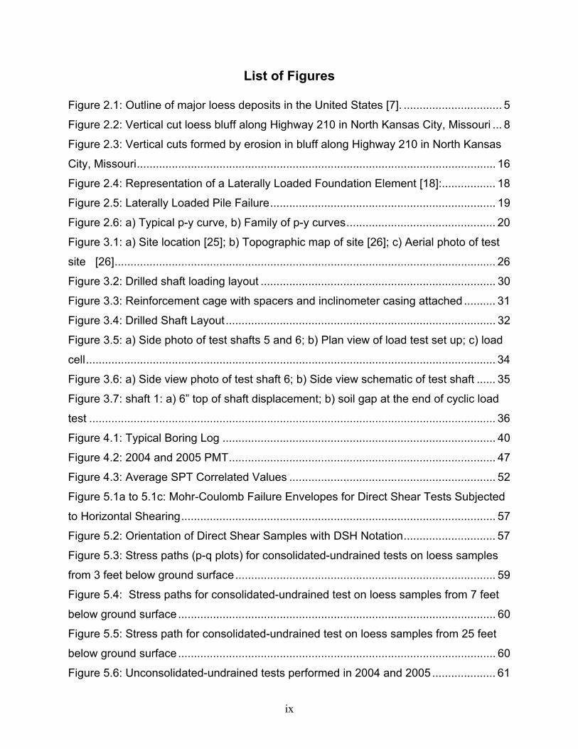
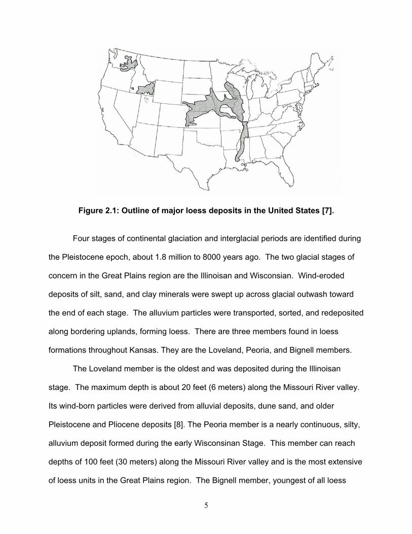
Figure 2.1: Outline of major loess deposits in the United States [7]. ............................... 5
Figure 2.2: Vertical cut loess bluff along Highway 210 in North Kansas City, Missouri ... 8
Figure 2.3: Vertical cuts formed by erosion in bluff along Highway 210 in North Kansas
City, Missouri................................................................................................................. 16
Figure 2.4: Representation of a Laterally Loaded Foundation Element [18]:................. 18
Figure 2.5: Laterally Loaded Pile Failure....................................................................... 19
Figure 2.6: a) Typical p-y curve, b) Family of p-y curves............................................... 20
Figure 3.1: a) Site location [25]; b) Topographic map of site [26]; c) Aerial photo of test
site [26]........................................................................................................................ 26
Figure 3.2: Drilled shaft loading layout .......................................................................... 30
Figure 3.3: Reinforcement cage with spacers and inclinometer casing attached .......... 31
Figure 3.4: Drilled Shaft Layout..................................................................................... 32
Figure 3.5: a) Side photo of test shafts 5 and 6; b) Plan view of load test set up; c) load
cell................................................................................................................................. 34
Figure 3.6: a) Side view photo of test shaft 6; b) Side view schematic of test shaft ...... 35
Figure 3.7: shaft 1: a) 6” top of shaft displacement; b) soil gap at the end of cyclic load
test ................................................................................................................................ 36
Figure 4.1: Typical Boring Log ...................................................................................... 40
Figure 4.2: 2004 and 2005 PMT.................................................................................... 47
Figure 4.3: Average SPT Correlated Values ................................................................. 52
Figure 5.1a to 5.1c: Mohr-Coulomb Failure Envelopes for Direct Shear Tests Subjected
to Horizontal Shearing................................................................................................... 57
Figure 5.2: Orientation of Direct Shear Samples with DSH Notation............................. 57
Figure 5.3: Stress paths (p-q plots) for consolidated-undrained tests on loess samples
from 3 feet below ground surface.................................................................................. 59
Figure 5.4: Stress paths for consolidated-undrained test on loess samples from 7 feet
below ground surface.................................................................................................... 60
Figure 5.5: Stress path for consolidated-undrained test on loess samples from 25 feet
below ground surface.................................................................................................... 60
Figure 5.6: Unconsolidated-undrained tests performed in 2004 and 2005 .................... 61

x
Figure 5.7: Mohr-Coulomb failure envelopes for triaxial compression tests .................. 62
Figure 5.8: Laboratory strength tests for samples obtained at 1 and 3 feet................... 63
Figure 5.9: Laboratory strength tests for samples obtained at 5 and 7 feet................... 64
Figure 5.10: Laboratory strength tests for samples obtained at 15 and 25 feet............. 65
Figure 5.11: Laboratory cohesion results for the soil profile. ......................................... 66
Figure 5.12: Laboratory friction angle results for the soil profile. ................................... 67
Figure 5.13: Anisotropic sample orientation for direct shear testing.............................. 68
Figure 5.14: Direct shear test results for specimens sampled at 1 foot ......................... 69
Figure 5.15: Direct shear test results for specimens sampled at 3 feet ......................... 69
Figure 5.16: Direct shear test results for specimens sampled at 5 feet ......................... 70
Figure 5.17: Direct shear test results for specimens sampled at 7 feet ......................... 70
Figure 5.18: Direct shear test results for specimens sampled at 15 feet ....................... 71
Figure 5.19: Direct shear test results for specimens sampled at 25 feet ....................... 71
Figure 5.20: Comparison of moduli for CPT and PMT soundings ................................. 72
Figure 5.21: Elastic modulus determined from in-situ and laboratory results ................ 73

1
Chapter 1
Introduction
Drilled shafts are a common type of deep foundation used when upper soils are weak or
subject to scour. They are capable of bearing large compressive or uplift forces as well
as large lateral loads. They are most commonly constructed by inserting a reinforcing
steel cage into a drilled hole and filling it with concrete. They are often used for bridge
foundations, retaining structures, and large highway signs on transportation projects.
Depending on the function, deep foundations must support axial loads, lateral
loads, and react against moments. Axial loads are transferred to the soil through side
friction and toe bearing resistance. Lateral loads can be static, such as water pressures
on piers or earth pressures on retaining walls, or dynamic, such as wave action through
soil due to earthquakes. Lateral loads produce lateral deflections through shear and
moment reactions and are transferred to adjacent soil through lateral bearing.
The lateral load-deformation relationship of a shaft and its interaction with
supporting soil must be evaluated when developing a safe and economical structural
design. Drilled shaft deflection depends on the soil response and the soil response is a
function of the shaft deflection. This soil-structure reaction is modeled as a p-y curve,
where p is the lateral soil resistance per unit length of the foundation and y is the lateral
deflection. Therefore, the p-y curve behavior is a function of both soil and foundation
properties. The p-y curve for a particular point on a foundation depends on soil type,
type of loading, foundation diameter and cross-sectional shape, coefficient of friction
between the foundation and the soil, and how the foundation was constructed [1].

2
The soil-structure interaction is modeled using a beam on elastic foundation
analysis, also known as the Winkler method. Through this method the soil is
represented by a series of independent nonlinear springs. Deformations of these
springs are the p-y curves. Thus, the foundation is represented using beam theory and
the soil resistance is represented by the p-y curves. The solution to the nonlinear p-y
curve takes the form of a fourth order differential equation that can easily be solved
using a computer program. Com624P and LPILE are two popular programs that model
lateral loads on foundations using a two-dimensional finite difference approach.
Com624P was the first widely used p-y analysis software [1], however LPILE is now
widely used and is the analysis tool used by the Kansas Department of Transportation
(KDOT). The p-y curves for this project were generated using LPILE.
Reese and others performed a majority of the load tests in the 1970’s [2]. They
correlated field and laboratory tests to derive a family of p-y curves for the lateral load
response in each of the following soils: soft clay, stiff clay, and sand above and below
the water table [2]. No family of p-y curves has been published from load tests in
loessial soils although Clowers and Frantzen conducted a full-scale lateral load test in
loessial soil on piles in the early 1990’s [3]. They concluded the soil-structure
interaction of loess was similar to sandy soils and the family of sandy soil p-y curves
could, therefore, be used in foundation design and analysis. However, loess has many
unique properties that set it apart from sandy soil. Much of the soil structure strength is
gained from clay and calcite cementation which can be lost due to a rise in moisture
content; the soil may also be susceptible to large settlements when saturated.
3
The purpose of this research was to define the significant engineering properties
of Kansas’ loessial soils through a literature review, laboratory tests, and in situ tests
and to determine the soil-structure response by constructing and testing a set of full-
scale drilled shafts. Laboratory tests were conducted in conjunction with KDOT on soil
specimens obtained from a total of eleven borings and two continuous soil samplings.
Laboratory testing consisted of: one dimensional consolidation, collapse, unconfined
compressive strength, unconsolidated-undrained triaxial, consolidated-undrained
triaxial, repeated loading triaxial, direct shear, and routine index testing. Field tests
included standard penetration tests (SPT), cone penetration tests (CPT), and
pressuremeter tests (PMT). Selected field tests were conducted in 2004 and during the
week of testing in 2005. The full scale load test included monitoring the behavior of six
laterally loaded drilled shafts. Shafts were subjected to static and repeated loads. The
soil-structure response of drilled shafts in loessial soils was analyzed to develop a
family of p-y curves.
4
Chapter 2
Literature Review
2.1 Loess
2.1.1 Origin
Multiple competing theories concerning the origin of loess have been proposed.
There are five different theories discussed in Loess, Lithology and Genesis [4];
however, nearly all authors accept and discuss the theory of an eolian origin in
textbooks and journal articles alike. Terzaghi, Peck, and Mesri define loess in general
as uniform, cohesive, wind-blown sediment [5]. Loess is a clastic soil mostly made of
silt-sized quartz particles and loosely arranged grains of sand, silt, and clay. Cohesion
is due to clay or calcite bonding between particles which are significantly weakened
upon saturation. When dry, loess has the unique ability to stand and support loads on
nearly vertical slopes.
Loess was formed during arid to semi-arid periods following the Pleistocene
continental glaciation. As the glaciers retreated, strong winds swept up sediments from
the outwash. Larger particles were sorted and deposited near the original riverbeds
while silt-size particles were transported downwind. The glacial till continued to be
swept up and reworked throughout the arid times, creating a loosely arranged soil
mass. Loess is present in central parts of the United States, Europe, the former Soviet
Union, Siberia, and in large parts of China and New Zealand [6]. Within the United
States, major loess deposits are found in Nebraska, Kansas, Iowa, Wisconsin, Illinois,
Tennessee, Mississippi, southern Idaho, and Washington, as mapped on figure 2.1 [7].
5
Figure 2.1: Outline of major loess deposits in the United States [7].
Four stages of continental glaciation and interglacial periods are identified during
the Pleistocene epoch, about 1.8 million to 8000 years ago. The two glacial stages of
concern in the Great Plains region are the Illinoisan and Wisconsian. Wind-eroded
deposits of silt, sand, and clay minerals were swept up across glacial outwash toward
the end of each stage. The alluvium particles were transported, sorted, and redeposited
along bordering uplands, forming loess. There are three members found in loess
formations throughout Kansas. They are the Loveland, Peoria, and Bignell members.
The Loveland member is the oldest and was deposited during the Illinoisan
stage. The maximum depth is about 20 feet (6 meters) along the Missouri River valley.
Its wind-born particles were derived from alluvial deposits, dune sand, and older
Pleistocene and Pliocene deposits [8]. The Peoria member is a nearly continuous, silty,
alluvium deposit formed during the early Wisconsinan Stage. This member can reach
depths of 100 feet (30 meters) along the Missouri River valley and is the most extensive
of loess units in the Great Plains region. The Bignell member, youngest of all loess
6
members, was deposited during the late Wisconsinan Stage. It is largely made of
reworked Peoria loess. The member is generally discontinuous and can reach depths
of 35 feet (10.6 meters) along the Missouri River valley. A layer of soil identified as the
Brady soil separates the Peoria and Bignell members. It was established during a brief
pause in loess formation and is widespread but discontinuous. Sangamon soils formed
between the Illinosian and Wisconsian periods and are found above beds of Loveland
loess [6 - 14]. These soils formed during interglacial periods differ from loess in that
they were products of worldwide climatic factors, not local erosion or deposition. In
Table 2.1, Bandyopadhyay presents a pictorial representation of the Pleistocene
stratigraphy layers in Kansas [6].
The major drainageways that produced Kansas’ loess members were the
Republican River valley in the north, the Smoky Hill River valley in north-central and
western Kansas, and the Missouri River valley for the extreme northeastern border of
Kansas. During the dry, warm weather following glacial retreat, northeastern Kansas
was predominantly mixed woodland and prairie while western Kansas was dominated
by short grasses and subject to strong winds. Due to the woodland wind barriers, loess
deposits in northeastern Kansas are thicker than western Kansas deposits and not as
uniform. Here, open terrains allowed the wind to deposit, pick-up, and rework silt
particles. This secondary source of deposition produced thinner, well-sorted, uniform
loess members [9].

7
2.1.2 Geotechnical Characteristics
Several characteristics are used to separate loess from other silty soils. In its
natural state, loess has an open, cohesive particle structure with low density and high
dry strength. Non-cohesive silty or clayey soils similar to loess in particle size,
deposition, and open particle arrangement are not considered loess. They are
considered wind-deposited silts, fine sands, or clays. Loess has a metastable structure
due to the high degree of settlement and large loss of strength that may occur upon
saturation. Gibbs and Holland clearly express the importance of understanding the
geotechnical aspects of loess [7]. They state:
Because of the unstable properties of loess which may cause settlement
of foundations of structures, such knowledge of the limitations of loess for
engineering purposes is important not only to the geologist and soil
Table 2.1 Pleistocene Stratigraphy in Kansas [6]
Time – Stratigraphy 1.8 million to 8000 years
ago Rock - Stratigraphy
Recent Stage Low Terraces and Alluvium Bignell Loess
Fluvial Deposits Brady Soils
Peoria Loess Wisconsinan Stage
Fluvial Deposits Sangamonian Stage Sangamon Soils
Loveland Loess Illinoisan Stage Fluvial Deposits
Yarmouthian Stage Yarmouth Soils Pearlette Ash Bed Kansan Stage
Fluvial and Eolian Deposits Till Aftonian Stage Afton Soils
Nebraskan Stage Fluvial and Eolian Deposits Till Oldest
Youngest
8
mechanics engineer but also to design and construction engineers who
are required to build structures on loessial soils [7].
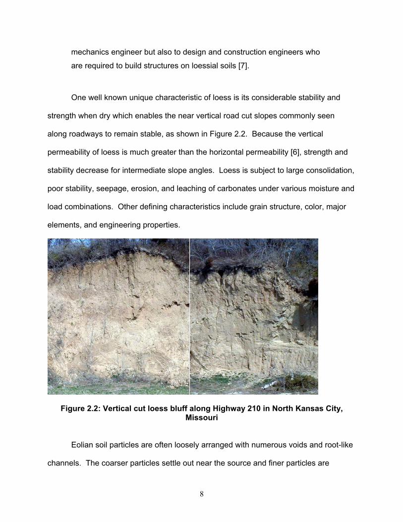
One well known unique characteristic of loess is its considerable stability and
strength when dry which enables the near vertical road cut slopes commonly seen
along roadways to remain stable, as shown in Figure 2.2. Because the vertical
permeability of loess is much greater than the horizontal permeability [6], strength and
stability decrease for intermediate slope angles. Loess is subject to large consolidation,
poor stability, seepage, erosion, and leaching of carbonates under various moisture and
load combinations. Other defining characteristics include grain structure, color, major
elements, and engineering properties.
Figure 2.2: Vertical cut loess bluff along Highway 210 in North Kansas City, Missouri
Eolian soil particles are often loosely arranged with numerous voids and root-like
channels. The coarser particles settle out near the source and finer particles are
9
deposited progressively further away. Therefore, local differences occur in the type and
quantity of mineral content. In general, the fabric of loess consists of fine, loosely
arranged angular grains of silt, fine sand, calcite, and clay. Most of the grains are
coated with thin films of clay and some with a mixture of calcite and clay. It is often
classified as a silty clay loam or a silt loam [6]. For Peoria loess, Swineford and Frye
noted a strong relationship between particle size and the degree of sorting. Coarser
samples are generally better sorted than the finer ones [9].
The granular components of loess are quartz, feldspars, volcanic ash shards,
carbonates, and micas. The percent of composition varied with each site sampled, but
in general quartz makes up around half the total volume of the deposit. [7, 15]
Color and particle size are strong identifiers of loess. It is commonly a buff,
medium to coarse-grained silt with fine to very fine grains of sand. In general, the
median grain size ranges from 0.00083-0.002 in. (0.02-0.05 mm) [9]. Thus, the average
grain size is smaller than the upper limit of silt, 0.0029 in. (0.074 mm). The Loveland
member is dark brown at the bottom and a very distinctive reddish brown at the top.
The greatest amount of sand is near the bottom of the member. Peoria and Bignell
members are light yellowish brown or buff. They are well sorted near the river bluffs
and the range of particle size varies with distance [9, 13, 14, 16].
Calcite is believed to be a major cementing material in loess. It can be leached
into the soil from above or can be brought into the soil by evaporation of capillary water
from the groundwater below. However, clay is more commonly the bonding agent that
gives loess its cohesive nature. Bandyopadhyay found montmorillonite clay to be the
major cementing material in Kansas loess, while calcite “usually occurs in distinct silt-

10
sized grains throughout the loess in a finely dispersed state rather than as a cementing
material [6].” Gibbs and Holland found that, in general, intergranular supports were
composed mostly of montmorillonite clay with small amounts of illite [7]. They contend
that carbonates and clays react differently in water; therefore, if calcite was the main
cementing material, loess would not subside, consolidate, or lose strength as rapidly as
it does. Most often, calcite serves as a secondary support structure and clay as the
primary soil matrix [7].
Montmorillonite, kaolinite, and illite have all been identified in samples in Kansas
[8] along with calcite, quartz, and feldspars [15]. Crumpton and Badgley studied the
clay content in Kansas [8]. They found the clay content generally decreased with
increasing depth and decreased from east to west. With regard to the general loess
formation, there is an increase in clay content with increasing depth. The Loveland
member contains more clay than the Peoria and Bignell members. Loveland and
Peoria members are separated by the Sangamon soil, which also shows increasing
percent clay with increasing depth. The mineral types discussed are consistent for all
three members [8, 9, 15].
Montmorillonite and mixed layers of montmorillonite and illite are the cementing
material for the soil. These clay particles coat the host silt grains and the walls of
various holes forming the inter-granular support structure and serve as the matrix.
These supports give dry loess its impressive strength, stability, and ability to withstand
large loads with little settlement in the arid regions of the Midwest. As moisture content
increases, clay particles swell and bond strength is greatly reduced. There is a potential
for the soil matrix to collapse and extensive settlement to occur. With high vertical
11
permeability due to large voids and vertical root holes, moisture quickly dissipates and
loess remains dry. If it overlies less permeable materials such as clayey shale and
retains water, the bond strength and soil structure will weaken upon saturation.
Sheeler researched quantitative properties of loess, including specific gravity,
Atterberg limits, permeability, density, shear strength, and natural moisture content as
shown in Table 2.2 [16].
Specific gravity is influenced by local variations in the type and quantity of
mineral content. Values range from 2.57 to 2.78, as shown in Table 2.2. The average
value is 2.66 [6, 7, 16], which is similar to the typical value of clean, light colored quartz
sand.
The Plasticity Indices for loess range from 5 to 37 and the Liquid Limits range
from 25 to 60 depending on the amount of clay present [7, 8, 16]. High Plasticity Index
values correspond to high percentages of montmorillonite in the soil [6].
Permeability is influenced by soil properties such as particle size and shape,
gradation, void ratio and continuity, and soil structure [14]. It is a widely varied local
feature with in-place vertical permeabilities of loess ranging from 10 to over 1000 ft/yr (1
x10-5 to 1 x10⁻³ cm/s), determined after consolidation was complete under a given load
[16]. Bandyopadhyay states the vertical permeability of Peoria loess in Kansas in on
the order of 900 ft/yr (9 x10⁻⁴ cm/s) and is much larger than the horizontal permeability.
“[The higher vertical permeability] is partly due to the existence of vertical tubules and
shrinkage joints within the soil mass [6].” Terzaghi viewed permeability in loess as an
elusive property because the structure changes when it is saturated. It breaks down,
becomes denser, and its permeability is decreased [16].
12
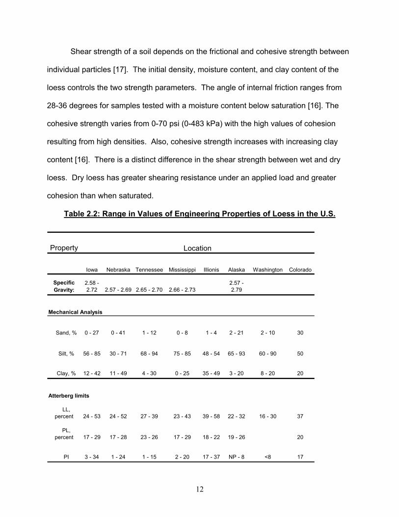
Shear strength of a soil depends on the frictional and cohesive strength between
individual particles [17]. The initial density, moisture content, and clay content of the
loess controls the two strength parameters. The angle of internal friction ranges from
28-36 degrees for samples tested with a moisture content below saturation [16]. The
cohesive strength varies from 0-70 psi (0-483 kPa) with the high values of cohesion
resulting from high densities. Also, cohesive strength increases with increasing clay
content [16]. There is a distinct difference in the shear strength between wet and dry
loess. Dry loess has greater shearing resistance under an applied load and greater
cohesion than when saturated.
Table 2.2: Range in Values of Engineering Properties of Loess in the U.S.
Property
Iowa Nebraska Tennessee Mississippi Illionis Alaska Washington Colorado
Specific Gravity:
2.58 - 2.72 2.57 - 2.69 2.65 - 2.70 2.66 - 2.73
2.57 - 2.79
Sand, % 0 - 27 0 - 41 1 - 12 0 - 8 1 - 4 2 - 21 2 - 10 30
Silt, % 56 - 85 30 - 71 68 - 94 75 - 85 48 - 54 65 - 93 60 - 90 50
Clay, % 12 - 42 11 - 49 4 - 30 0 - 25 35 - 49 3 - 20 8 - 20 20
LL, percent 24 - 53 24 - 52 27 - 39 23 - 43 39 - 58 22 - 32 16 - 30 37
PL, percent 17 - 29 17 - 28 23 - 26 17 - 29 18 - 22 19 - 26 20
PI 3 - 34 1 - 24 1 - 15 2 - 20 17 - 37 NP - 8 <8 17
Location
Mechanical Analysis
Atterberg limits
13
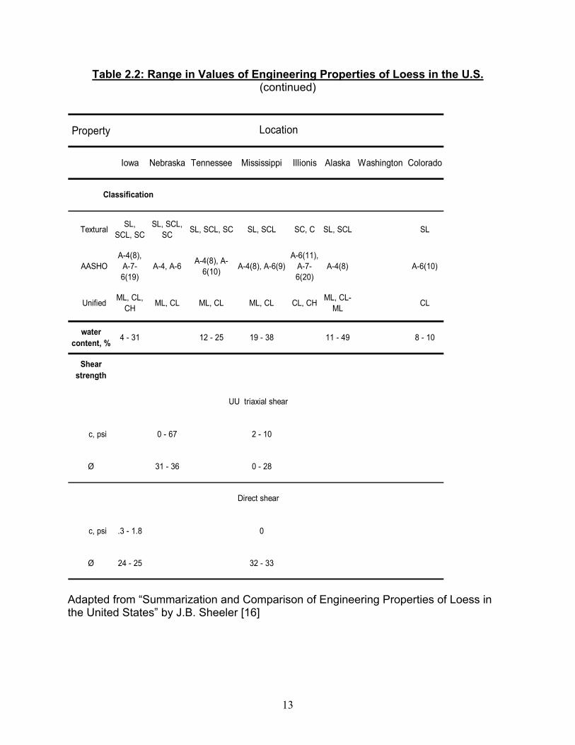
Table 2.2: Range in Values of Engineering Properties of Loess in the U.S. (continued)
Property
Iowa Nebraska Tennessee Mississippi Illionis Alaska Washington Colorado
Textural SL, SCL, SC
SL, SCL, SC SL, SCL, SC SL, SCL SC, C SL, SCL SL
AASHOA-4(8),
A-7-6(19)
A-4, A-6 A-4(8), A-6(10) A-4(8), A-6(9)
A-6(11), A-7-6(20)
A-4(8) A-6(10)
Unified ML, CL, CH ML, CL ML, CL ML, CL CL, CH ML, CL-
ML CL
water content, % 4 - 31 12 - 25 19 - 38 11 - 49 8 - 10
Shear strength
c, psi 0 - 67 2 - 10
Ø 31 - 36 0 - 28
c, psi .3 - 1.8 0
Ø 24 - 25 32 - 33
Location
Classification
UU triaxial shear
Direct shear
Adapted from “Summarization and Comparison of Engineering Properties of Loess in the United States” by J.B. Sheeler [16]
14
Loess is often associated with terms such as “collapse,” “hydroconsolidation,” or
“hydrocompaction [6].” Consolidation may be the most outstanding physical and
structural property of loess. Its susceptibility to settlement makes it a potentially
unstable foundation material. Because of the reaction between montmorillonite and
moisture, slight variations in clay content and moisture content may cause collapse and
consolidation. An increase in moisture content may cause clay bonds to weaken,
reducing the original soil strength. Saturated loess consolidates under lower stress
conditions than when dry. Therefore, an increase in moisture content is often a more
important contributor to collapse and consolidation than loading [7, 21].
Bandyopadhyay found that:
Soils susceptible to hydroconsolidation can be identified by a density criterion – that is, if density is sufficiently low to give a space larger than needed to hold the liquid-limit water content, collapse problems on saturation are likely [6].
In general, settlement will be large for loess with dry unit weights below 80 pounds per
cubic foot (pcf) and small for those exceeding 90 pcf (1.28 g/cm3 and 1.44 g/cm3,
respectively) [6, 7]. Therefore, loessial soils with low field densities and clay
cementation can be expected to have a high consolidation and collapse potential [6].
Observed dry unit weights of loessial soils vary from 66-104 pcf (1.06-1.67 g/cm3)
[16]. For the Bignell loess member, unit weight varies from 75-90 pcf (1.20-1.44 g/cm3).
Peoria members typically have unit weights around 85 pcf (1.36 g/cm3) or less.
Therefore, as previously discussed, Peoria loess can suffer great settlement. Loveland
loess generally has a denser fabric, unit weights from 90-104 pcf (1.44-1.67 g/cm3)
because of increased clay content and is less susceptible to large settlements [6].
15
The ultimate bearing capacity of a soil is the bearing pressure required such that
shear stresses induced by a footing just exceed shear strength of the soil [14]. For dry
loess, bearing capacity may exceed 10,000 pounds per square foot (psf) (480 kPa) but
may drop to 500 psf (24 kPa) upon saturation.
In-situ moisture contents of loess range from 4 to 49%. There is a strong
correlation between regional average annual rainfall and the natural moisture content.
Because the structure of loess is loosely arranged and filled with voids, rainfall quickly
infiltrates and loess may remain dry within a few feet of the surface, unless there is a
water table near the surface. Gibbs and Holland concluded that maximum dry strength
occurs at moisture contents below 10%, and high resistance to settlement should be
expected. Soils with moisture contents between 10 to 15% have moderately high
strength, with strength declining as moisture approaches 20%. Moisture contents
above 20% are considered high and will permit full consolidation to occur under load.
Saturation occurs at about 35% moisture [7].
Loess has very little resistance to erosion by flowing water because of the
softening of clay bonds. Therefore, erosion is the main force in creating naturally
occurring vertical cuts in loess, shown in Figure 2.3.
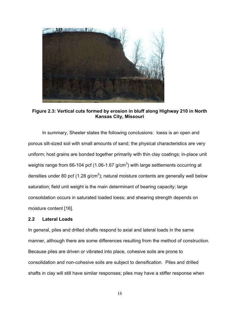
16
Figure 2.3: Vertical cuts formed by erosion in bluff along Highway 210 in North Kansas City, Missouri
In summary, Sheeler states the following conclusions: loess is an open and
porous silt-sized soil with small amounts of sand; the physical characteristics are very
uniform; host grains are bonded together primarily with thin clay coatings; in-place unit
weights range from 66-104 pcf (1.06-1.67 g/cm3) with large settlements occurring at
densities under 80 pcf (1.28 g/cm3); natural moisture contents are generally well below
saturation; field unit weight is the main determinant of bearing capacity; large
consolidation occurs in saturated loaded loess; and shearing strength depends on
moisture content [16].
2.2 Lateral Loads
In general, piles and drilled shafts respond to axial and lateral loads in the same
manner, although there are some differences resulting from the method of construction.
Because piles are driven or vibrated into place, cohesive soils are prone to
consolidation and non-cohesive soils are subject to densification. Piles and drilled
shafts in clay will still have similar responses; piles may have a stiffer response when

17
placed in sandy soils [18]. Additionally, cement will migrate into the adjacent soil during
construction of drilled shafts, causing an increase in stiffness of the surrounding soil.
The stiffness increase is small and the estimated response of the soil is considered to
be equivalent for both drilled shafts and piles [3, 18].
Careful consideration should be given to the nature of lateral loads on piles and
drilled shafts. Potential types of loading include short-term, repeated, sustained, and
seismic or dynamic. Short-term, or static, loading is often used in field tests to correlate
the soil response with its engineering properties. Sustained loads come from retaining
walls or bridge abutments. Traffic on a curved bridge, currents or waves, and ice are
examples of repeated loads. Dynamic loads can come from machinery vibrations and
earthquakes [2].
Foundation deflection due to lateral loading is a function of both the foundation
properties and the soil response. Likewise, the soil response depends on soil
properties and the foundation reaction. This soil-structure interaction is modeled as a
nonlinear beam on elastic foundation. The model assumes the soil is a continuous,
isotropic, and elastic medium. The drilled shaft or pile is divided into equally spaced
sections and the soil response is modeled by a series of closely spaced discrete springs
called Winkler’s springs, shown in Figure 2.4 [18].
Because the foundation is divided into sections, the soil response at a point is
independent of pile deflection elsewhere and a continuum is not perfectly modeled.
This discrepancy is minor and a means for correction is included in COM624P [2].
While horizontal beams-on-foundation use conventional bearing capacity for shallow
foundations to determine the ultimate resistance of the soil, pu, laterally loaded
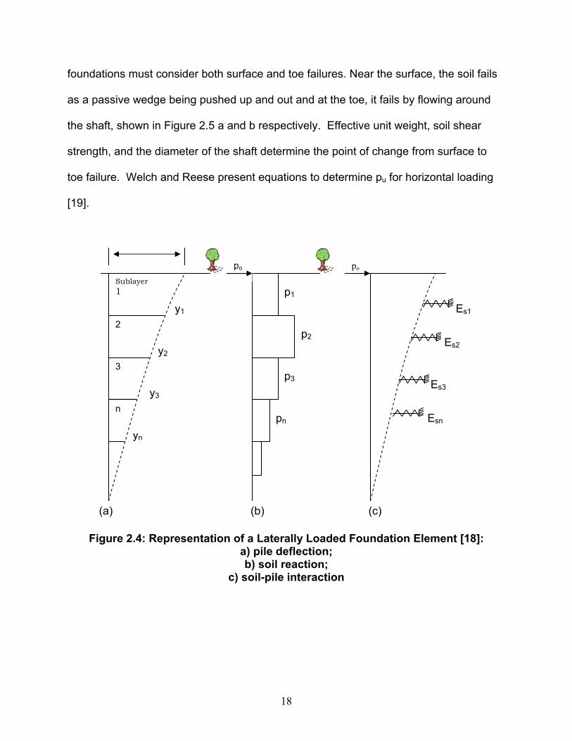
18
foundations must consider both surface and toe failures. Near the surface, the soil fails
as a passive wedge being pushed up and out and at the toe, it fails by flowing around
the shaft, shown in Figure 2.5 a and b respectively. Effective unit weight, soil shear
strength, and the diameter of the shaft determine the point of change from surface to
toe failure. Welch and Reese present equations to determine pu for horizontal loading
[19].
Figure 2.4: Representation of a Laterally Loaded Foundation Element [18]:
a) pile deflection; b) soil reaction;
c) soil-pile interaction
Esn
Es3
Es2
Es1
yn
y3
y2
y1 p1
p2
p3
pn
yo po
3
2
n
Sublayer 1
(a) (c)
po
(b)

19
(a) (b)
Figure 2.5: Laterally Loaded Pile Failure [19]: a) Surface Failure;
b) Toe Failure
2.3 Beam Theory
For beam theory, a fourth order differential equation, based on the basic beam slope
equation, is used to derive a mathematical expression for the soil resistance, p, against
foundation deflection, y. This is described below [18, 19]:
Ø = dy/dx …………………….………………………………………… (2.1)
M = EI dØ/dx = EI d2y/dx2 …….……………………………………… (2.2)
Where M/EI = d2y/dx2 is the basic equation for curvature of a bent beam.
V = dM/dx = EI d3y/dx3 ………...……………………………………… (2.3)
p = dV/dx = EI d4y/dx4 ……………………………...…………………. (2.4)
The notation is as follows:
Ø = slope of the beam (radians)
M = moment in the beam (in-lb.)
V = shear in the beam (lb.)
p = soil reaction against the beam (lb. /in.)
x = distance along the axis of the beam (in.)
y = deflection of the beam perpendicular to the axis (in.)
20
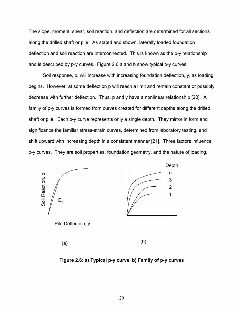
The slope, moment, shear, soil reaction, and deflection are determined for all sections
along the drilled shaft or pile. As stated and shown, laterally loaded foundation
deflection and soil reaction are interconnected. This is known as the p-y relationship
and is described by p-y curves. Figure 2.6 a and b show typical p-y curves.
Soil response, p, will increase with increasing foundation deflection, y, as loading
begins. However, at some deflection p will reach a limit and remain constant or possibly
decrease with further deflection. Thus, p and y have a nonlinear relationship [20]. A
family of p-y curves is formed from curves created for different depths along the drilled
shaft or pile. Each p-y curve represents only a single depth. They mirror in form and
significance the familiar stress-strain curves, determined from laboratory testing, and
shift upward with increasing depth in a consistent manner [21]. Three factors influence
p-y curves. They are soil properties, foundation geometry, and the nature of loading.
Figure 2.6: a) Typical p-y curve, b) Family of p-y curves
Es
Pile Deflection, y
Soi
l Rea
ctio
n, p
(a)
Depth n 3 2 1
(b)
21
There are many equations relating soil resistance, p, and deflection, y, with the
soil stress-strain properties determined in a lab or measured in the field. The general
formula is [19]:
p/pu = 0.5 (y/y50)n ..…………………………………………………..……(2.5)
where n depends on the soil. For stiff clay above the water table, n equals ¼.
For soft clay below the water table, n equals ⅓ [19]. Duncan and others developed p-y
curves for partly saturated silts and clays. They presented “the general form of the
cubic parabola relationship” [20] as:
p = 0.5 pu [y/(Aε50D)]n …………………………………………..…………[2.6]
where n equals ⅓, A is a coefficient that controls the magnitude of deflections, D
is the diameter or width of the pile or drilled shaft, and ε50 is the strain required to
mobilize 50% of the soil strength. Reese and Matlock recommend using triaxial
compression tests, with confining pressure equal to the overburden pressure, for
determining the shear strength of sand above and below the water table. “Values
obtained from the triaxial tests might be somewhat conservative but would represent
more realistic strength values than other tests [19].” Matlock recommended in-situ
vane-shear tests and unconsolidated-undrained triaxial compression tests for soft clays
below the water table. The values of shear strength, c, and strain should be taken at
one-half the maximum total principal stress difference.
The ratio of p to y is expressed as the soil modulus of the pile reaction, Es (lb/in3).
Es = - p/y ……………………………………………………………….(2.7)
p = - Es y ………………………………………………………………..(2.8)
22
Mathematically, it is the slope of the p-y curve and will usually increase with
depth. At a given depth it will become smaller as pile deflection increases because of
the nonlinear relationship of p and y. Es represents the stiffness of the Winkler springs,
shown in figure 2.6 d and e.
Axial loads are usually the primary form of loading on foundations, and will affect
the response to horizontal loading on drilled shafts and piles. Welch and Reese clearly
explain that “the application of a horizontal load or a moment reduces the axial stiffness
of the element. The flexural stiffness is reduced by axial compression and increased by
axial tension [18].” Therefore, the new fourth order differential equation to consider
includes a constant axial force, P. The equation is:
EI d4y/d4x + P d2y/dx2 + Es y = 0 ………………………………..……..(2.9)
The derivation of equation 2.9 is given in the Com624P manual along with the
solutions for soft and stiff clay, sand, and layered systems [19].
Initial p-y analyses came from full-scale load tests. Lateral load tests were
performed by the following people in the indicated soils: soft clay by Matlock in 1970;
stiff clay by Welch, Reese and others in 1972 and 1975; sand by Cox, Reese, and
Grubbs in 1974; vuggy limestone by Reese and Nyman in 1978 [19]. This type of
analysis is expensive and most accurate for the exact soil it was performed in.
However, using experienced engineering judgment, the p-y curves generated can be
extrapolated to fit other soil types.
Com624P uses soil parameters and incremental structural loads to find a
condition of static equilibrium and compute the shear, moment, and lateral deflection at
each interval [1]. For all soil types, the basic input parameters include the soil effective
23
unit weights, γ’, and the horizontal subgrade modulus, k. For cohesive soils, the
parameters include the cohesion, cu, and the measured strain and 50% of the maximum
principal stress. For cohesionless soils and cohesive soils under drained conditions, the
parameter includes the internal friction angle, Ø. The soil parameters are obtained for
laboratory tests or correlations using the results from field tests. Anderson, Townsend,
and Grajales concluded that the standard penetration test (SPT) correlation based
predictions were conservative while the cone penetration tests (CPT) best-predicted
field behavior. The DMT derived p-y curves predicted performance well at low loads and
the pressuremeter test (PMT) derived p-y curve predicted performance well for sands
and clays [22].
Another method of analysis often used begins with assuming a point of zero
deflection on the drilled shaft or pile. This is called the point-of-fixity. Slope, moment,
and deflection can be determined through superposition for different points along the
pile or drilled shaft. However, it is nearly impossible to accurately assume the point-of-
fixity. Therefore, a conservative estimation of its location must be made.
24
Chapter 3
Scope of Research
The strength of loess and its resistance to lateral forces depends primarily on its clay
content, moisture content, and dry unit weight. Even though these are highly regional
properties, Swineford and Frye found that:
[P]properties of the loess, especially those of the Nebraska and Kansas area, are
sufficiently similar to establish certain important generalized findings for resolving
soil mechanics and foundation problems [12].
Therefore, by relating a full scale load test with soil parameters obtained from in-
situ and laboratory tests, a pertinent soil-structure relationship can be established.
Multiple load tests were conducted as a part of this research under the conditions
described in this chapter.
3.1 Site Investigation
A uniform deposit of loess located on the northwest corner of I-435 and highway 32 in
Wyandotte County, Kansas was selected by the University of Kansas (KU) and KDOT
for the full scale lateral load test. Figure 3.1 shows the location of the test. In the early
1990’s, Frantzen and Clowers [3] performed a full scale load test on cast-in-place piles
on the north bound side of I-435, shown in the northeast corner of Figure 3.2, opposite
the current test site. The site, which is part of the Loveland member, was chosen for its
deep, uniform deposit of loess and deep groundwater table.
The soil profile consisted of tan to brown, silty, sandy clay to clayey and sandy
silt. Water contents decreased after 12 feet below the surface; the soil was dry and stiff
25
below 16 feet boring termination. Ten borings were drilled by KDOT using a CME-45
truck. Nine were drilled during June of 2004 and one was drilled June of 2005 during
the week of load testing. KDOT located the borings in the field and provided relative
location information.
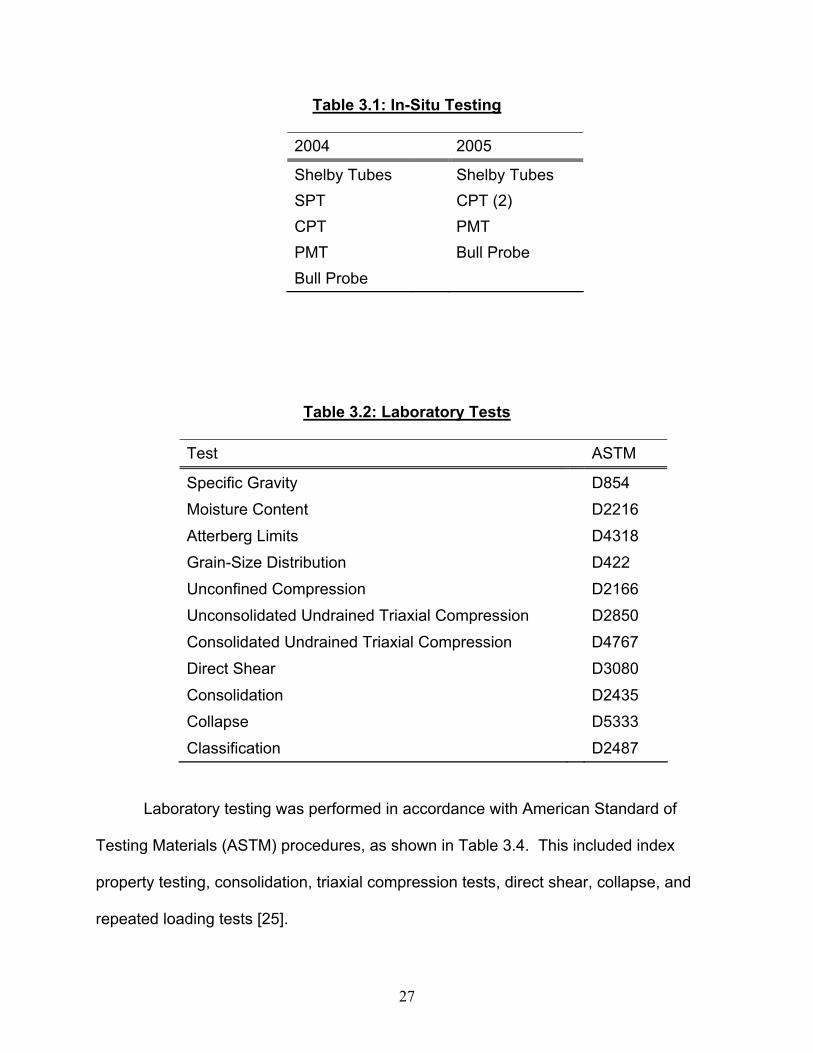
Field tests included standard penetration tests (SPT) in Borings A-D using an
automatic hammer, a total of three cone penetration tests (CPT), two pressuremeter
tests (PMT), and two continuous soil profiles obtained using a bull probe sampler,
shown in Table 3.3. The PMT tests were performed using a Rocktest pressuremeter,
model G-AM, at depths of 2, 5, and 10 feet. All in-situ tests performed in 2005 were
conducted within two days of the final lateral load test to provide the most accurate soil
profile possible when determining the soil’s response to loading. Undisturbed soil was
sampled using 3.5 inch diameter, thin-walled shelby tubes. The tubes were
hydraulically advanced to depths of 1, 5, 7, 15, 23, and 25 feet on average. Boring logs
are presented in Appendix B detailing at what depths each test was performed and
shelby tubes were taken for each of the ten borings.
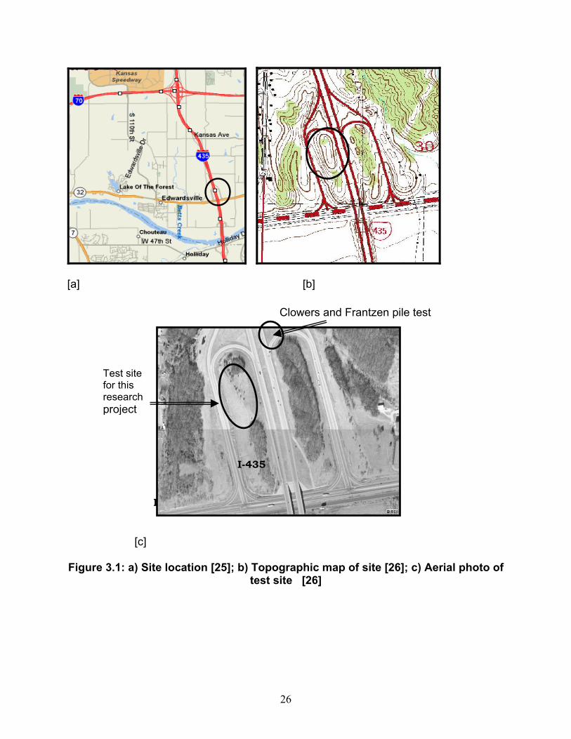
26
[a] [b]
[c]
Figure 3.1: a) Site location [25]; b) Topographic map of site [26]; c) Aerial photo of test site [26]
Hwy 32
Test site for this research project
Clowers and Frantzen pile test
I-435
27
Table 3.1: In-Situ Testing
2004 2005
Shelby Tubes Shelby Tubes SPT CPT (2) CPT PMT PMT Bull Probe Bull Probe
Table 3.2: Laboratory Tests
Test ASTM
Specific Gravity D854 Moisture Content D2216
Atterberg Limits D4318 Grain-Size Distribution D422
Unconfined Compression D2166 Unconsolidated Undrained Triaxial Compression D2850
Consolidated Undrained Triaxial Compression D4767 Direct Shear D3080
Consolidation D2435 Collapse D5333
Classification D2487
Laboratory testing was performed in accordance with American Standard of
Testing Materials (ASTM) procedures, as shown in Table 3.4. This included index
property testing, consolidation, triaxial compression tests, direct shear, collapse, and
repeated loading tests [25].
28
KDOT performed laboratory tests on undisturbed 2.8 inch diameter samples
trimmed from 3.5 inch shelby tubes. KU performed laboratory tests on 1.4 inch
diameter samples. Testing smaller samples caused more variations in the test results;
however, it conserved enough sample to test for anisotropy within each shelby tube.
The 1.4 inch sample sets were carved for unconsolidated undrained triaxial
compression and direct shear so the long axis was in the vertical and horizontal
direction. Comparisons were made at 1, 5, and 24 feet below the surface.
3.2 Test Shafts
3.2.1 Configuration and Construction
Drilled shaft dimensions and test configurations were based on the
recommendations of Dan Brown and Associates. The expected soil response was
estimated using laboratory results to determine the amount of concrete reinforcement
required. Test shafts 1 and 2 were 42 inches in diameter; shafts 3, 4, 5, and 6 were 30
inches in diameter. The total design length of 27 feet was determined so the shafts
were longer than the estimated point-of-fixity. Approximately 3.15 feet of the total length
was cased above ground to facilitate application of the lateral load. Shafts were spaced
12 feet on center in all directions. Table A.1 in Appendix A lists as-built dimensions and
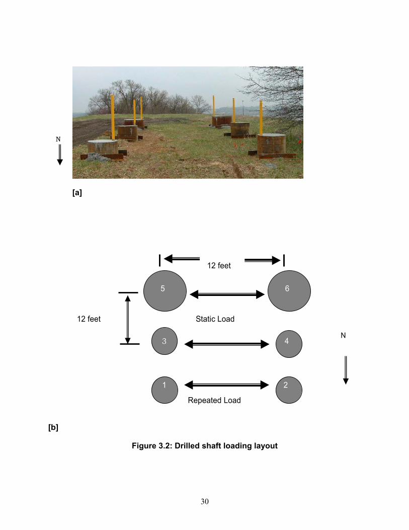
details of all test shafts. Shafts were designed to react against each other under static
and repeated loading as shown in Figure 3.2. Inclinometer casings were installed the
full length of all six test shafts. Table A.2 in Appendix A shows as-built dimensions of
the inclinometer casings.
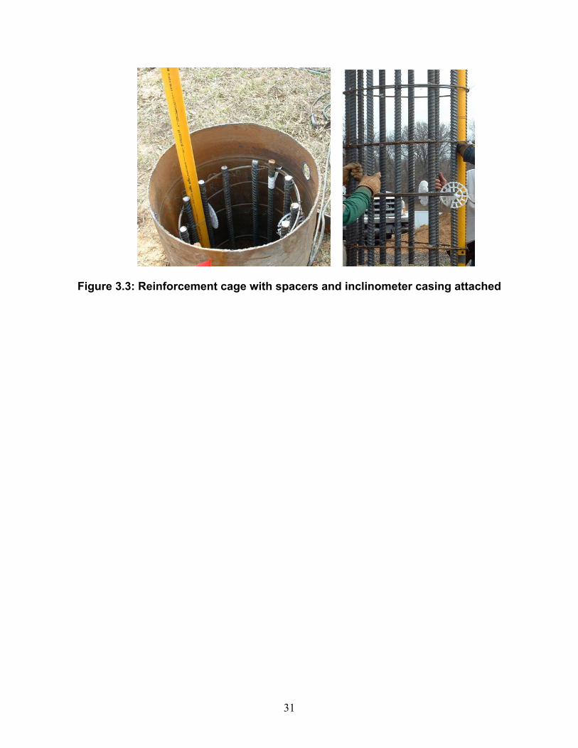
Drilled shafts were constructed in a typical dry excavation manner. The 30-inch
holes were drilled first. Spacers were added to the outside of each rebar cage to
29
ensure the cages were centered upon installation. Inclinometer casings were attached
to the inside of each cage, shown in Figure 3.3. The reinforcement was then lowered
into place and concrete was poured. Concrete specifications and strengths are shown
in Appendix A, Table A3 and Figure A4, respectively. After construction, the shafts
were allowed to cure for 70 days prior to loading.
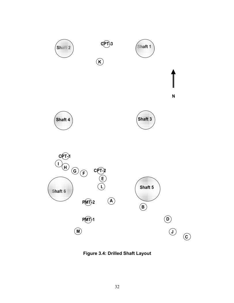
Figure 3.4 relates the six drilled shafts to the location of in-situ tests performed
and borings drilled. Locations were plotted approximately to scale. Borings A through I
were drilled in 2004 and boring J was drilled in 2005, one day after the final load test
was completed.
30
[a]
Static Load
12 feet
12 feet
5 6
3 4
Repeated Load
1 2
N
[b]
Figure 3.2: Drilled shaft loading layout
NN
31
Figure 3.3: Reinforcement cage with spacers and inclinometer casing attached
32
K
L
CPT-2
D
C
A
PMT-1
IH
G FE
CPT-1
B
Shaft 6Shaft 5
Shaft 3Shaft 4
Shaft 1Shaft 2
JM
CPT-3
PMT-2
N
Figure 3.4: Drilled Shaft Layout
33
3.2.2 Instrumentation
A load cell, used to apply the compressive lateral force, and a hydraulic jack
were mounted inline between each pair of drilled shafts as shown in Figure 3.5 a and b.
The applied load was measured using a calibrated load cell that was attached to the
shaft by a steel collar as shown in Figure 3.5c. Two linear variable displacement
transducers, LVDTs, were mounted on each collar to measure the top of shaft
displacement. One LVDT was approximately 6 inches above and one was
approximately 6 inches below the point of load application, shown in Figure 3.6.
Shaft deflections were measured using inclinometer soundings. The first set of
inclinometer soundings were measured at ½ inch top of shaft displacement. At this
time, the inclinometer was oriented along the north – south groove inside the casing and
lowered into the drilled shaft. Readings were taken at two feet intervals for the length of
the shaft. The inclinometer was brought back to the surface, realigned along the east –
west groove inside the casing and again lowered into the drilled shaft. Readings were
taken at two feet intervals for the length of the shaft. This ended the first inclinometer
sounding.

34
[a]
[b]
[c]
Figure 3.5: a) Side photo of test shafts 5 and 6; b) Plan view of load test set up; c) load cell
LVDT
Reference Beam
Inclinometer Casing
LVDT
Reference Beam
Inclinometer Casing
Test Shaft
Load Cell
Load Cell
Pressure Feed
Hydraulic Jack
35
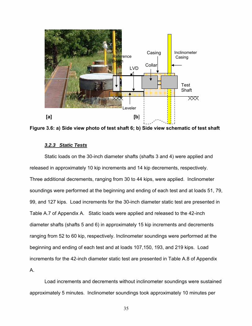
[a] [b]
Figure 3.6: a) Side view photo of test shaft 6; b) Side view schematic of test shaft
3.2.3 Static Tests
Static loads on the 30-inch diameter shafts (shafts 3 and 4) were applied and
released in approximately 10 kip increments and 14 kip decrements, respectively.
Three additional decrements, ranging from 30 to 44 kips, were applied. Inclinometer
soundings were performed at the beginning and ending of each test and at loads 51, 79,
99, and 127 kips. Load increments for the 30-inch diameter static test are presented in
Table A.7 of Appendix A. Static loads were applied and released to the 42-inch
diameter shafts (shafts 5 and 6) in approximately 15 kip increments and decrements
ranging from 52 to 60 kip, respectively. Inclinometer soundings were performed at the
beginning and ending of each test and at loads 107,150, 193, and 219 kips. Load
increments for the 42-inch diameter static test are presented in Table A.8 of Appendix
A.
Load increments and decrements without inclinometer soundings were sustained
approximately 5 minutes. Inclinometer soundings took approximately 10 minutes per
Collar
Inclinometer Casing
Test Shaft
Casing
LVD
Reference Beam
Leveler
36
shaft to perform; the total load duration was 20 minutes. Lateral pressures were
maintained for load increments without inclinometer soundings. The hydraulic pressure
was locked off during each sounding to better maintain deflected pile shape with depth.
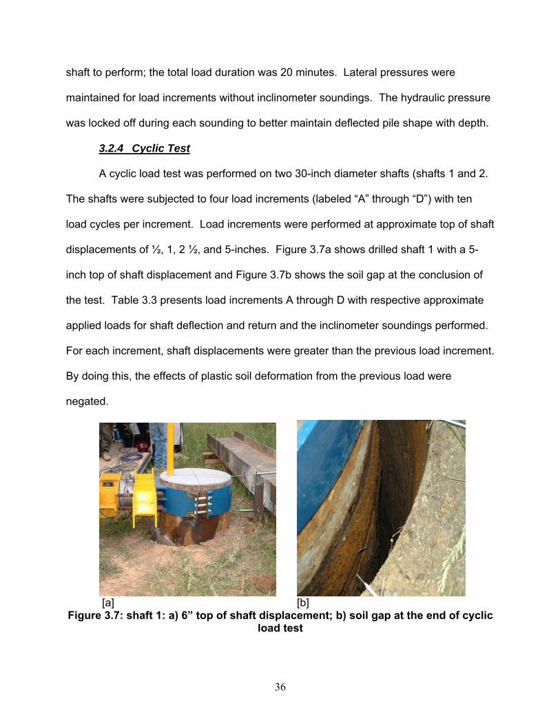
3.2.4 Cyclic Test
A cyclic load test was performed on two 30-inch diameter shafts (shafts 1 and 2.
The shafts were subjected to four load increments (labeled “A” through “D”) with ten
load cycles per increment. Load increments were performed at approximate top of shaft
displacements of ½, 1, 2 ½, and 5-inches. Figure 3.7a shows drilled shaft 1 with a 5-
inch top of shaft displacement and Figure 3.7b shows the soil gap at the conclusion of
the test. Table 3.3 presents load increments A through D with respective approximate
applied loads for shaft deflection and return and the inclinometer soundings performed.
For each increment, shaft displacements were greater than the previous load increment.
By doing this, the effects of plastic soil deformation from the previous load were
negated.
[a] [b]
Figure 3.7: shaft 1: a) 6” top of shaft displacement; b) soil gap at the end of cyclic load test
37
For each cycle, loads were sustained for only a few seconds and increment
durations (A through D) are presented in Table 3.11. Inclinometer soundings were
performed on the first and last cycles for each load increment (cycles 1 and 10);
therefore, loads were held for approximately 20 minutes. As with each static load test,
the hydraulic pressure was locked off during each inclinometer sounding to help
maintain deflected pile shape with depth.
Table 3.3: Load Increments for the 30-inch Diameter Cyclic Test
Load Increment
Increment Duration Load Cycles
(min) Deflect ReturnN/A N/A None 0 0
A 1 1 through 10 50 -15
B 2 1 through 10 79 -25
C 3.5 1 through 10 99 -30
D 6.5 1 through 10 127 -30
Inclinometer Soundings Performed
Approximate Load (kips)
Prior to Loading
at Load Cycles 1 and 10 for each Load Increment

38
Chapter 4
Test Results
Laboratory and field testing was performed to estimate engineering and index
properties of loess. Analytical results are presented in this chapter. Results of
laboratory tests are presented on boring logs in Appendix B. Laboratory and field test
results are presented in Appendix C.
4.1 Laboratory Results
KDOT conducted consolidated-undrained triaxial compression tests, unconsolidated-
undrained triaxial compression tests, and unconfined compressive strength tests on
samples 2.8 inches in diameter with a height to diameter ratio of approximately 2.2:1.
Direct shear, consolidation, and index property tests were also performed. Testing was
conducted on samples obtained in June 2004.
KU conducted unconsolidated-undrained triaxial compression tests on 1.4 inch
diameter samples with a 2:1 height to diameter ratio. KDOT and KU both performed
direct shear tests on 2.5 inch diameter samples. Pairs of samples tested in direct
shear, from the same depth, were trimmed such that shear planes of the samples were
parallel and perpendicular to the vertical effective field stress, respectively. This was
done to analyze anisotropic strength characteristics. Consolidation, collapse, and index
property testing were also conducted. Testing was conducted on samples collected in
2004 and 2005. Soil samples collected in 2005 were obtained during the week of load
testing.
39
Figure 4.1 shows a subsurface profile of the test site along with representative
soil parameters. The lithology and soil parameters presented are representative of all
13 borings. The SPT blow counts have been averaged within each sample from three
to four SPT tests at the same depths. N, N60, and N1(60) correlations are discussed in
section 4.2.3. Natural moisture content, Atterberg limits, and shear strength values are
from the 2004 Shelby tube samples.
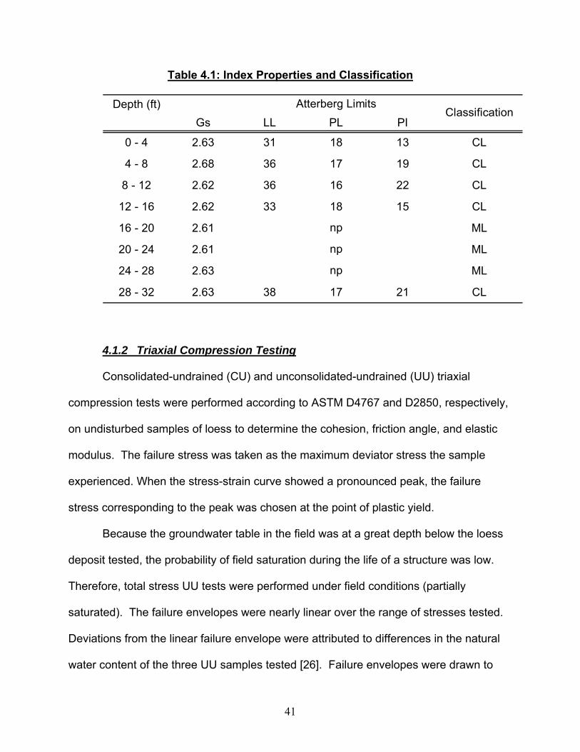
4.1.1 Index Properties
Standard characterization tests were conducted on the soil samples. These
included specific gravity, Atterberg limits, grain size distribution, and classification
according to the ASTMs listed in Table 3.2. Table 4.1 presents the results; grain size
distribution curves are shown in Appendix C.
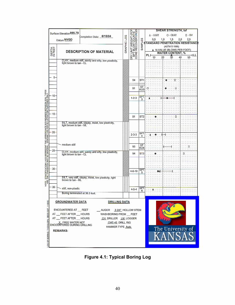
40
Figure 4.1: Typical Boring Log
41
Table 4.1: Index Properties and Classification
Depth (ft)Gs LL PL PI
0 - 4 2.63 31 18 13 CL
4 - 8 2.68 36 17 19 CL
8 - 12 2.62 36 16 22 CL
12 - 16 2.62 33 18 15 CL
16 - 20 2.61 ML
20 - 24 2.61 ML
24 - 28 2.63 ML
28 - 32 2.63 38 17 21 CL
np
Atterberg LimitsClassification
np
np
4.1.2 Triaxial Compression Testing
Consolidated-undrained (CU) and unconsolidated-undrained (UU) triaxial
compression tests were performed according to ASTM D4767 and D2850, respectively,
on undisturbed samples of loess to determine the cohesion, friction angle, and elastic
modulus. The failure stress was taken as the maximum deviator stress the sample
experienced. When the stress-strain curve showed a pronounced peak, the failure
stress corresponding to the peak was chosen at the point of plastic yield.
Because the groundwater table in the field was at a great depth below the loess
deposit tested, the probability of field saturation during the life of a structure was low.
Therefore, total stress UU tests were performed under field conditions (partially
saturated). The failure envelopes were nearly linear over the range of stresses tested.
Deviations from the linear failure envelope were attributed to differences in the natural
water content of the three UU samples tested [26]. Failure envelopes were drawn to
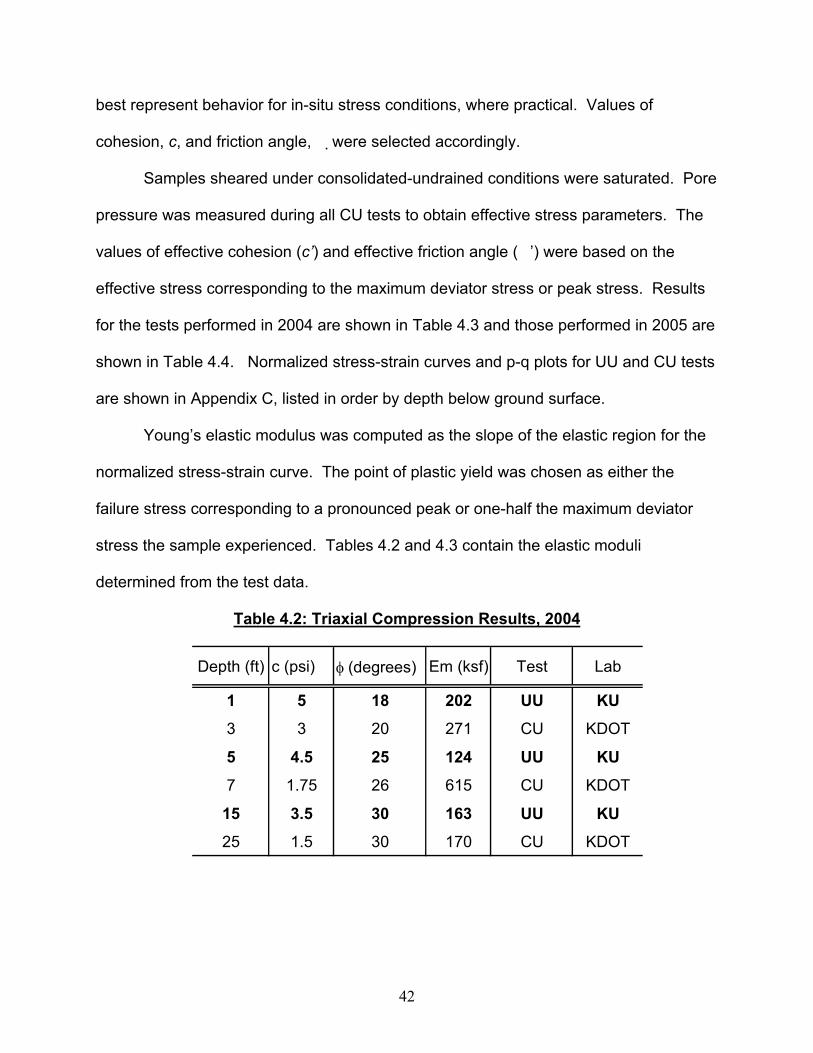
42
best represent behavior for in-situ stress conditions, where practical. Values of
cohesion, c, and friction angle, � were selected accordingly.
Samples sheared under consolidated-undrained conditions were saturated. Pore
pressure was measured during all CU tests to obtain effective stress parameters. The
values of effective cohesion (c’) and effective friction angle (�’) were based on the
effective stress corresponding to the maximum deviator stress or peak stress. Results
for the tests performed in 2004 are shown in Table 4.3 and those performed in 2005 are
shown in Table 4.4. Normalized stress-strain curves and p-q plots for UU and CU tests
are shown in Appendix C, listed in order by depth below ground surface.
Young’s elastic modulus was computed as the slope of the elastic region for the
normalized stress-strain curve. The point of plastic yield was chosen as either the
failure stress corresponding to a pronounced peak or one-half the maximum deviator
stress the sample experienced. Tables 4.2 and 4.3 contain the elastic moduli
determined from the test data.
Table 4.2: Triaxial Compression Results, 2004
Depth (ft) c (psi) φ (degrees) Em (ksf) Test Lab
1 5 18 202 UU KU
3 3 20 271 CU KDOT
5 4.5 25 124 UU KU
7 1.75 26 615 CU KDOT
15 3.5 30 163 UU KU
25 1.5 30 170 CU KDOT
43
Table 4.3: Triaxial Compression Results, 2005
Depth (ft) c (psi) φ (degrees) Em (ksf) Test Lab
1 4 22 152 UU KU
5 1.5 23 150 UU KU
15 0 32 228 UU KU
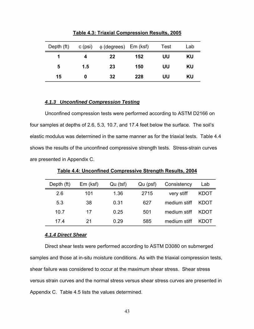
4.1.3 Unconfined Compression Testing
Unconfined compression tests were performed according to ASTM D2166 on
four samples at depths of 2.6, 5.3, 10.7, and 17.4 feet below the surface. The soil’s
elastic modulus was determined in the same manner as for the triaxial tests. Table 4.4
shows the results of the unconfined compressive strength tests. Stress-strain curves
are presented in Appendix C.
Table 4.4: Unconfined Compressive Strength Results, 2004
Depth (ft) Em (ksf) Qu (tsf) Qu (psf) Consistency Lab
2.6 101 1.36 2715 very stiff KDOT
5.3 38 0.31 627 medium stiff KDOT
10.7 17 0.25 501 medium stiff KDOT
17.4 21 0.29 585 medium stiff KDOT
4.1.4 Direct Shear
Direct shear tests were performed according to ASTM D3080 on submerged
samples and those at in-situ moisture conditions. As with the triaxial compression tests,
shear failure was considered to occur at the maximum shear stress. Shear stress
versus strain curves and the normal stress versus shear stress curves are presented in
Appendix C. Table 4.5 lists the values determined.

44
Table 4.5: Direct Shear Results, 2004
Depth vertical shear
horizontal shear
vertical shear
horizontal shear submerged lab
1 6.5 5 27 21 no KU
3 1.5 4 25 24 yes KDOT
5 1 1 23 24 no KU
7 0 1.5 27 27 yes KDOT
15 5.5 2 28 25 yes KDOT
25 2 0 22 21 no KU
c (psi) φ (degrees)
4.1.5 Consolidation and Collapse
Consolidation testing was performed at 3, 7, 15, and 24 feet below the surface.
Conventional fixed ring odometers were used with the Geocomp automated soil testing
system. Readings were automatically taken after consolidation was completed in
accordance with ASTM D2435 and loads were automatically applied when 100%
consolidation was achieved. The initial load increment was 1/8 tsf and loads were
doubled with each application up to 16 tsf. One rebound curve was plotted for each test
where the load was taken from 16 tsf to ¼ tsf, dropping by 4 tsf per increment. Table
4.6 presents the consolidation parameters determined and Appendix C has the void
ratio verses the log of pressure curves.
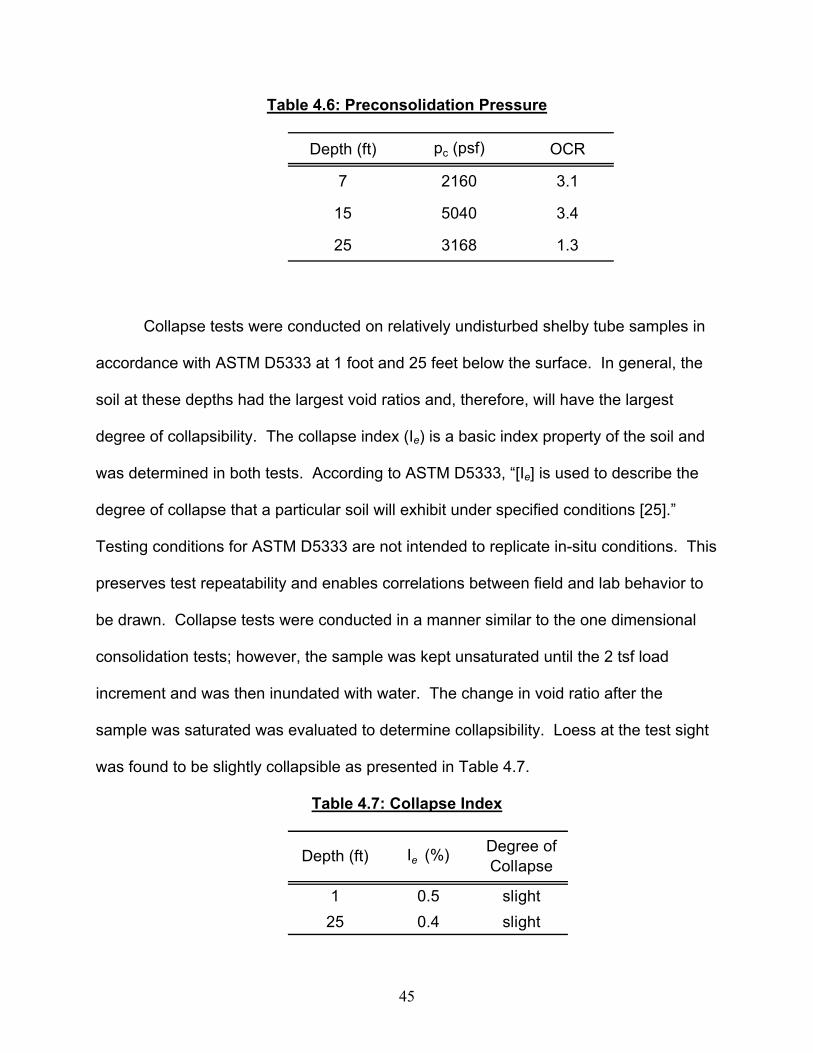
45
Table 4.6: Preconsolidation Pressure
Depth (ft) pc (psf) OCR
7 2160 3.1
15 5040 3.4
25 3168 1.3
Collapse tests were conducted on relatively undisturbed shelby tube samples in
accordance with ASTM D5333 at 1 foot and 25 feet below the surface. In general, the
soil at these depths had the largest void ratios and, therefore, will have the largest
degree of collapsibility. The collapse index (Ie) is a basic index property of the soil and
was determined in both tests. According to ASTM D5333, “[Ie] is used to describe the
degree of collapse that a particular soil will exhibit under specified conditions [25].”
Testing conditions for ASTM D5333 are not intended to replicate in-situ conditions. This
preserves test repeatability and enables correlations between field and lab behavior to
be drawn. Collapse tests were conducted in a manner similar to the one dimensional
consolidation tests; however, the sample was kept unsaturated until the 2 tsf load
increment and was then inundated with water. The change in void ratio after the
sample was saturated was evaluated to determine collapsibility. Loess at the test sight
was found to be slightly collapsible as presented in Table 4.7.
Table 4.7: Collapse Index
1 0.5 slight25 0.4 slight
Degree of Collapse
Ie (%)Depth (ft)
46
4.2 In-Situ Testing
Field testing included PMT, CPT, Shelby tubes, and a continuous soil profile taken from
a bull sampler as presented in Table 3.1. The continuous soil profile was presented in
the representative boring log on Figure 4.1. Parameters needed for p-y curves are not
directly obtained from the tests but can be estimated using correlated parameters
presented in this section.
4.2.1 Pressuremeter Test
Three pressuremeter tests were conducted by KDOT, two in 2004 and one
during the week of the full scale load test in 2005. Tests were performed at depths of 2,
5, and 10 feet below the ground surface. Table 4.8 lists the values recorded and Figure
4.2 shows the difference between the 2004 and 2005 tests. Figures of each test are
shown individually in Appendix C. The following two equations were used to determine
the elastic modulus (Em) and the at-rest earth pressure coefficient [5]:
Epm = 2(1+ν)(V0+vm)(Δp/Δv) …………………………………………………… 4.1
Where vm =(vo + vf) / 2
Epm = pressuremeter elastic modulus
ν = Poisson’s ratio = 0.33
V0 = initial volume of pressuremeter cell
Δp = change in pressure corresponding to αv
Δv = change in volume corresponding to αp
Em = Epm/ α ……………………………………………………………………….4.2
Where α = 0.5
The at rest earth pressure coefficient was calculated as the horizontal stress
divided by the vertical overburden stress.
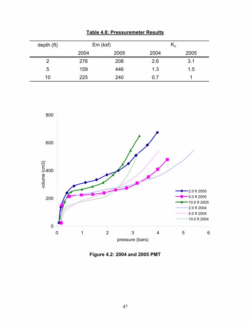
47
Table 4.8: Pressuremeter Results
depth (ft)2004 2005 2004 2005
2 276 208 2.6 3.15 159 446 1.3 1.5
10 225 240 0.7 1
Em (ksf) Ko
0
200
400
600
800
0 1 2 3 4 5 6pressure (bars)
volu
me
(cm
3)
2.0 ft 20055.0 ft 200510.0 ft 20052.0 ft 20045.0 ft 200410.0 ft 2004
Figure 4.2: 2004 and 2005 PMT
48
4.2.2 Cone Penetration Test
KDOT performed three CPT tests; one in 2004 and two during the week of the
lateral load test. The software used to collect and analyze the field data was CPT-LOG
Ver. 2.15a and CPT-pro Ver. 5.22, respectively. Figure 3.6 shows the location of the
CPT tests in relation to the testing shafts. CPT logs are presented in Appendix C.
There are two soil profiles; one was computerized and the other was conducted
manually by KU. The computer generated profile contains several layers of gravelly
sand. However, the soil profiles obtained from the continuous bull sampler and from
laboratory testing indicated the soil was silt to sandy silt with no gravel present.
Therefore, KU performed a CPT profile analysis using correlations derived from
Robertson & Campanella[28]. These figures are presented in Appendix C.
The correlation by Schmertmann [30] was used to determine the elastic modulus
and the correlation by Kulhawy and Mayne [32] was used to determine the effective
friction angle of the soil. The equations are as follows:
Em = 2 * qc (ksf) …………………………….…………………………….……. 4.3
Φ’= tan-1 (0.1 + 0.38 * log (qc / σz’)) ……………………………………………. 4.4
Table 4.9 and 4.10 show the results from the KU CPT analysis for 2004 and
2005 respectively.
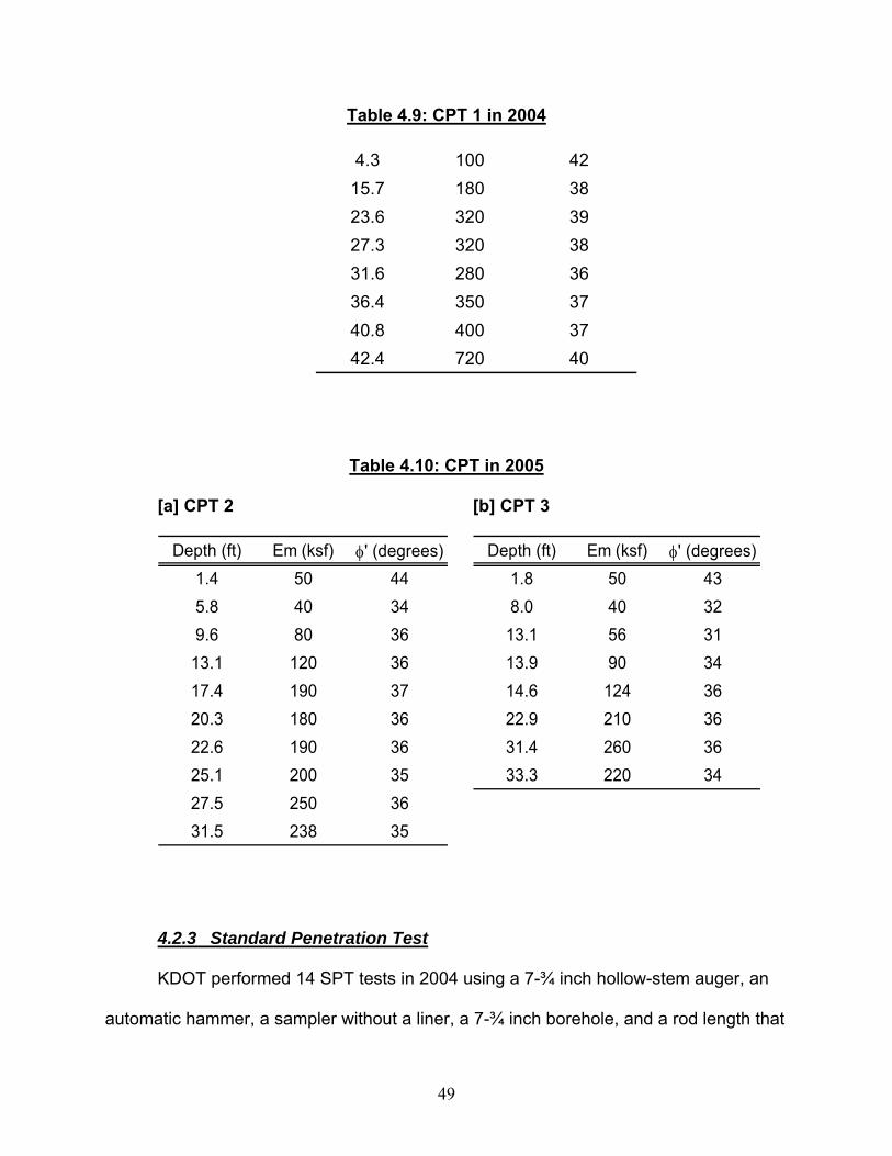
49
Table 4.9: CPT 1 in 2004
4.3 100 4215.7 180 3823.6 320 3927.3 320 3831.6 280 3636.4 350 3740.8 400 3742.4 720 40
Table 4.10: CPT in 2005
[a] CPT 2 [b] CPT 3
Depth (ft) Em (ksf) φ' (degrees)1.4 50 445.8 40 349.6 80 3613.1 120 3617.4 190 3720.3 180 3622.6 190 3625.1 200 3527.5 250 3631.5 238 35
Depth (ft) Em (ksf) φ' (degrees)1.8 50 438.0 40 32
13.1 56 3113.9 90 3414.6 124 3622.9 210 3631.4 260 3633.3 220 34
4.2.3 Standard Penetration Test
KDOT performed 14 SPT tests in 2004 using a 7-¾ inch hollow-stem auger, an
automatic hammer, a sampler without a liner, a 7-¾ inch borehole, and a rod length that
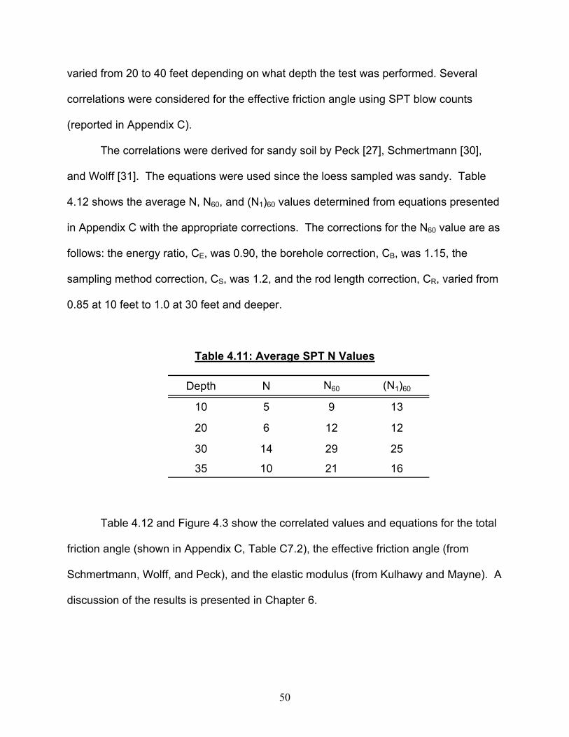
50
varied from 20 to 40 feet depending on what depth the test was performed. Several
correlations were considered for the effective friction angle using SPT blow counts
(reported in Appendix C).
The correlations were derived for sandy soil by Peck [27], Schmertmann [30],
and Wolff [31]. The equations were used since the loess sampled was sandy. Table
4.12 shows the average N, N60, and (N1)60 values determined from equations presented
in Appendix C with the appropriate corrections. The corrections for the N60 value are as
follows: the energy ratio, CE, was 0.90, the borehole correction, CB, was 1.15, the
sampling method correction, CS, was 1.2, and the rod length correction, CR, varied from
0.85 at 10 feet to 1.0 at 30 feet and deeper.
Table 4.11: Average SPT N Values
Depth N N60 (N1)60
10 5 9 13
20 6 12 12
30 14 29 25
35 10 21 16
Table 4.12 and Figure 4.3 show the correlated values and equations for the total
friction angle (shown in Appendix C, Table C7.2), the effective friction angle (from
Schmertmann, Wolff, and Peck), and the elastic modulus (from Kulhawy and Mayne). A
discussion of the results is presented in Chapter 6.
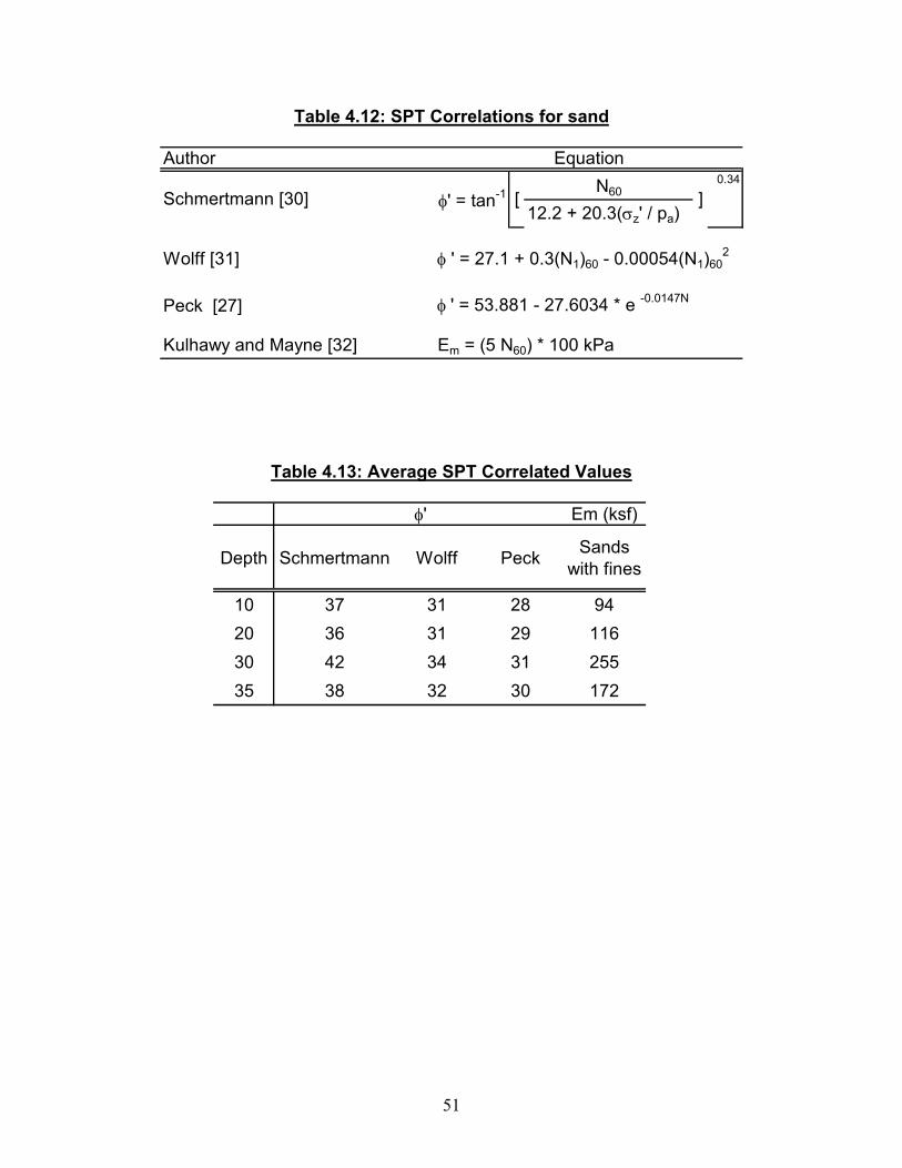
51
Table 4.12: SPT Correlations for sand
Author0.34
12.2 + 20.3(σz' / pa)
Wolff [31]
Peck [27] φ ' = 53.881 - 27.6034 * e -0.0147N
Kulhawy and Mayne [32]
Schmertmann [30] φ' = tan-1 [N60
Em = (5 N60) * 100 kPa
φ ' = 27.1 + 0.3(N1)60 - 0.00054(N1)602
Equation
]
Table 4.13: Average SPT Correlated Values
Em (ksf)
Depth Schmertmann Wolff Peck Sands with fines
10 37 31 28 9420 36 31 29 11630 42 34 31 25535 38 32 30 172
φ'
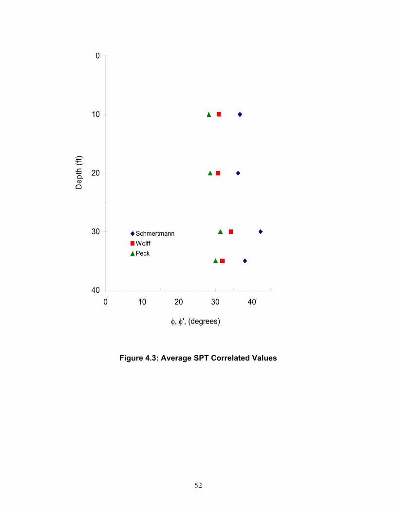
52
0
10
20
30
400 10 20 30 40 50
φ, φ', (degrees)
Dep
th (f
t)
SchmertmannWolffPeck
Figure 4.3: Average SPT Correlated Values
53
Chapter 5
Analysis and Comparison of Laboratory and In-Situ Testing
The use of accurate, and even elaborate, methods of testing requires no
justification in the research laboratory. The extent to which these methods
should be adopted in routine testing depends largely on whether or not
they reduce the margin of uncertainty in design sufficiently to justify their
cost. [25]
Most empirical geotechnical correlations are for soils categorized as sand or clay.
Loess has some of the characteristics of both sand and clay. In this chapter, field and
laboratory results are compared along with empirical correlations to determine which
correlations best suit loess.
5.1 Soil Classification
Soil from the site was classified by laboratory and in-situ methods. A visual
classification, based on split spoon samples, Atterberg limits, and shear strength
testing, is presented on boring logs in Appendix B.
The soil was classified based on laboratory testing as low plasticity clay (CL)
from the ground surface to a depth of 16 feet. The soil was classified as non-plastic to
low plasticity silt (ML) from 16 to 28 feet below the surface. The soil was again classified
as low plasticity clay (CL) from 28 to 32 feet below the surface.
The soil was classified in-situ using a computer generated CPT profile. Three
different CPT tests were performed. CPT analyses 1 and 3 indicated a clay layer
approximately 9 to 12 feet thick just below the ground surface. This CPT method does

54
not distinguish between high and low plasticity clay. Below the clay layer, the
computerized CPT analysis indicates alternating layers of silty sand, sandy silt, and
clayey silt. CPT analysis 2 presents a soil profile consisting of alternating layers of
sand, clayey sand, gravely sand, and no silt. CPT 1 was located on the south side of
the test site, between drilled shafts 4 and 6. CPT 2 was also located on the south side,
between shafts 5 and 6. CPT 3 was located on the north side of the test site, between
shafts 1 and 2. Test 1 and 3 were on opposite sides of the test site and had similar
computer generated soil profiles. Test 1 and 2 were around the same test shaft, shaft
6, but had a large discrepancy in the computer generated soil profile (see Figures C6.1,
6.3, and 6.4 in Appendix C).
A CPT analysis was performed manually using correlations from Robertson and
Campanella [28]. These profiles consisted of alternating layers of sand, silty sand, and
sandy silt, see Figures C6.1, 6.3, and 6.4 in Appendix C. The soil profile produced is
more consistent with the laboratory classification but still differs significantly from actual
soil samples. It was concluded that samples are required to obtain the most reliable soil
classification information for loessial soils.
These results suggest that soil classification in loess deposits based on CPT
correlations can vary significantly based on the correlation used and confirmation of soil
type through borings is recommended.
5.2 Direct Shear
The direct shear test is the oldest method for investigating the shearing strength of soils
[5]. Samples were tested under submerged and in-situ conditions to analyze the effect
of increasing moisture on strength and cohesion. All samples quickly consolidated
55
before testing began and submerged samples were sheared at a rate to achieve
drained conditions. Using Coulomb’s strength equation,
s = c + σ’ tan Φ’ ………………………………………………………....5.1
critical combinations of shearing and normal stresses were plotted to create Mohr-
Coulomb failure envelopes for selected depths. True failure envelopes that extend over
a wide range of normal stresses are often curved under a given set of conditions;
however it is common practice to approximate the overall failure with a linear
relationship by assuming the soil parameters (c, Φ) are constant. Shear strengths were
plotted in Figure 5.1 up to the maximum overburden stress of the samples tested using
equation 5.1.
In-situ sample orientation for direct shear laboratory tests is shown in Figure 5.2.
Samples were tested to replicate in-situ shear where the shearing plane is parallel to
the vertical stress in the field are denoted DSV. Submerged tests, performed by KDOT,
were conducted on samples obtained from shelby tubes taken at depths of 3, 7, and 15
feet. Submerged tests are noted by (s) in the following figures. Samples taken at 1, 5,
and 25 feet below the ground surface were tested at in-situ conditions by KU.
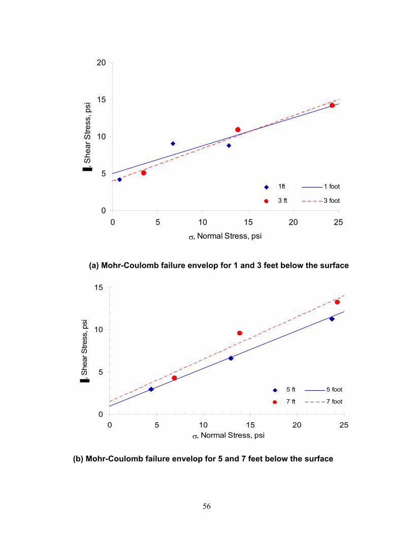
56
0
5
10
15
20
0 5 10 15 20 25
σ, Normal Stress, psi
, She
ar S
tress
, psi
1ft 1 foot
3 ft 3 foot
(a) Mohr-Coulomb failure envelop for 1 and 3 feet below the surface
0
5
10
15
0 5 10 15 20 25σ, Normal Stress, psi
, She
ar S
tress
, psi
5 ft 5 foot
7 ft 7 foot
(b) Mohr-Coulomb failure envelop for 5 and 7 feet below the surface

57
0
5
10
15
20
25
0 5 10 15 20 25 30 35 40 45
σ, Normal Stress, psi
, She
ar S
tress
, psi
15 ft 15 foot
25 ft 25 foot
(c) Mohr-Coulomb failure envelop for 15 and 25 feet below the surface
Figure 5.1a to 5.1c: Mohr-Coulomb Failure Envelopes for Direct Shear Tests Subjected to Horizontal Shearing
Figure 5.2: Orientation of Direct Shear Samples with DSH Notation
Cohesion generally decreased with depth. However, submerged samples from
depths of 7 and 15 feet were less cohesive than soils sampled at a depth of 25 feet and
tested at in-situ moisture conditions. Shear strength tended to decrease with depth for
samples tested under both submerged and in-situ moisture conditions.
5.3 Triaxial Compression
Stress-strain curves developed under unconsolidated-undrained and
consolidated-undrained triaxial compression testing conditions were similar to stress-
58
strain curves of sandy material with sufficient normal stress to not induce sample
expansion. Terzaghi states:
(that) to interpret laboratory or field strength tests and to select strength
parameters for stability analysis, it is useful to examine the manner in
which the effective normal stress and the shear stress change during
mobilization of the shearing resistance [5].
Stress paths were plotted for all triaxial compression tests performed. Figures
5.3, 5.4, and 5.5 contain the stress paths of the three consolidated-undrained tests
performed on samples taken from 3, 7, and 25 feet below the ground surface,
respectively. All samples were consolidated under isotropic pressure conditions. Pore
water pressure was measured and total and effective stress paths were plotted, p-q and
p’-q, respectively. P and p’ were determined from consolidated-undrained triaxial
compression tests performed by KDOT in 2004. Triaxial test results are presented in
Appendix C. p and q were calculated from (σ1 + σ 3) / 2 and (σ 1 - σ 3) / 2, respectively.
p’ and q’ include effects from pore water pressure, calculated as (σ 1’ + σ 3’) / 2 and q =
q’, respectively.
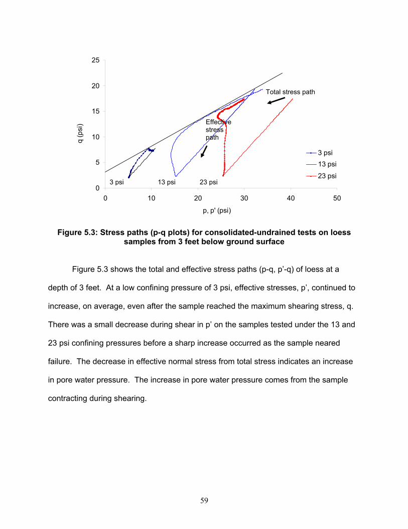
59
0
5
10
15
20
25
0 10 20 30 40 50
p, p' (psi)
q (p
si)
3 psi13 psi
23 psi
Figure 5.3: Stress paths (p-q plots) for consolidated-undrained tests on loess samples from 3 feet below ground surface
Figure 5.3 shows the total and effective stress paths (p-q, p’-q) of loess at a
depth of 3 feet. At a low confining pressure of 3 psi, effective stresses, p’, continued to
increase, on average, even after the sample reached the maximum shearing stress, q.
There was a small decrease during shear in p’ on the samples tested under the 13 and
23 psi confining pressures before a sharp increase occurred as the sample neared
failure. The decrease in effective normal stress from total stress indicates an increase
in pore water pressure. The increase in pore water pressure comes from the sample
contracting during shearing.
Total stress path
Effective stress path
3 psi 13 psi 23 psi
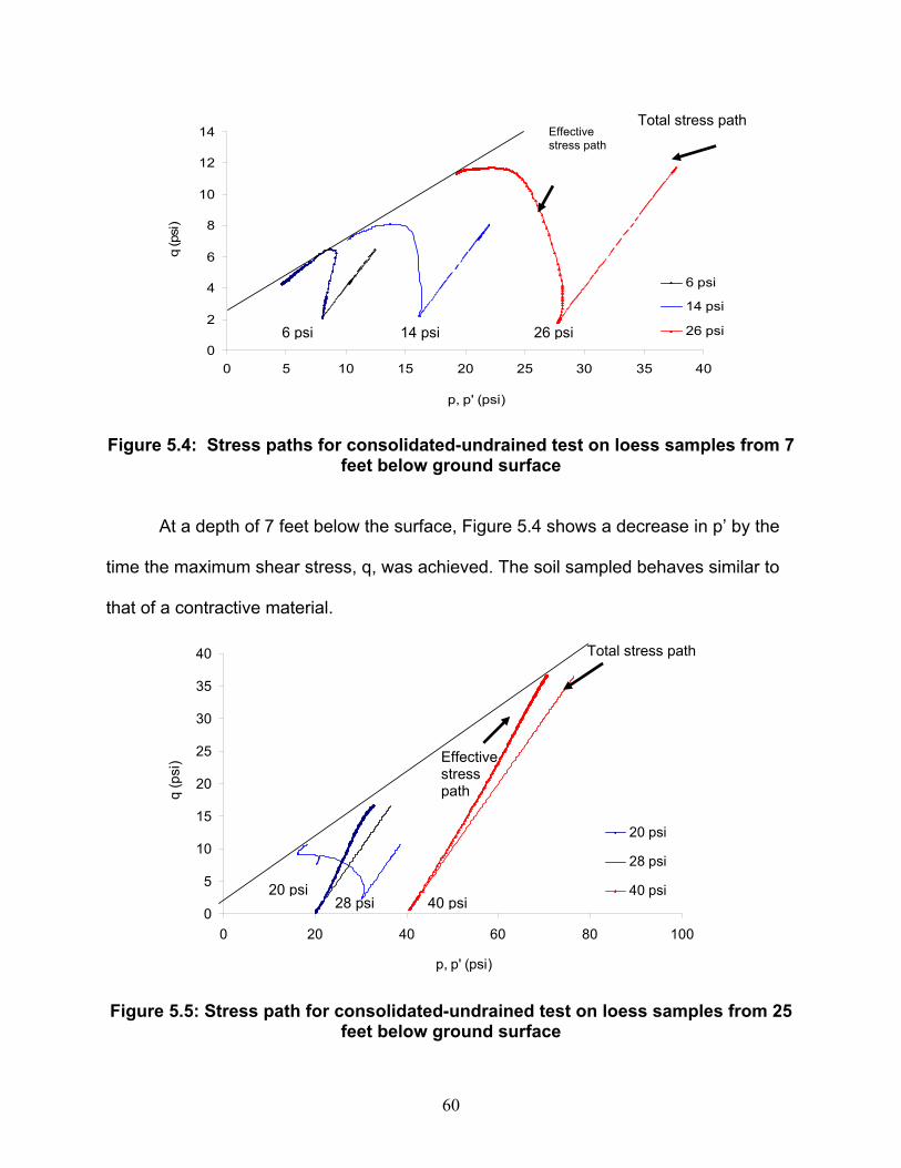
60
0
2
4
6
8
10
12
14
0 5 10 15 20 25 30 35 40
p, p' (psi)
q (p
si)
6 psi
14 psi
26 psi
Figure 5.4: Stress paths for consolidated-undrained test on loess samples from 7 feet below ground surface
At a depth of 7 feet below the surface, Figure 5.4 shows a decrease in p’ by the
time the maximum shear stress, q, was achieved. The soil sampled behaves similar to
that of a contractive material.
0
5
10
15
20
25
30
35
40
0 20 40 60 80 100
p, p' (psi)
q (p
si)
20 psi
28 psi
40 psi
Figure 5.5: Stress path for consolidated-undrained test on loess samples from 25 feet below ground surface
Total stress path Effective stress path
6 psi 14 psi 26 psi
Total stress path
Effective stress path
20 psi 28 psi 40 psi

61
Figure 5.5 is similar to Figure 5.1 in that p’ continued to increase as the shear
strength increases (20 and 40 psi samples), but the gap between p and p’ increased for
each case, indicating increased pore pressure for all samples. For the sample tested at
a confining pressure of 28 psi, p’ decreased as the sample began to shear. This
indicates the sample contracted as it sheared, similar to a loose sand. Therefore, the
soil profile, from depths of 3-25 feet, is contractive.
Soils sampled at 1, 5, and 15 feet below the ground surface were sheared under
unconsolidated, undrained conditions. Tests at each depth were conducted on samples
obtained in 2004 and during the week of the load test in 2005. Figure 5.6 shows the
difference in cohesion and friction angles between the two tests at each depth.
0
5
10
15
20
0 3 6 9 12 15normal stress (psi)
shea
r stre
ngth
(psi
)
1 ft UU, 2004
1 ft UU, 2005
5 ft UU, 2004
5 ft UU, 2005
15 ft UU, 2004
15 ft UU, 2005
Figure 5.6: Unconsolidated-undrained tests performed in 2004 and 2005
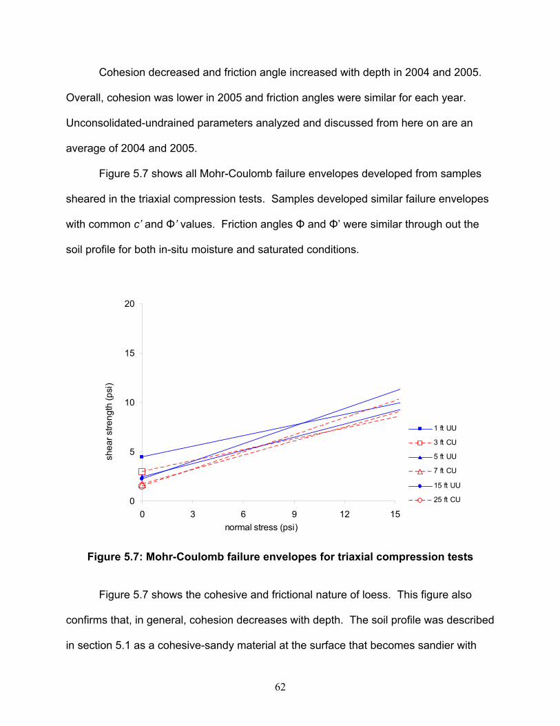
62
Cohesion decreased and friction angle increased with depth in 2004 and 2005.
Overall, cohesion was lower in 2005 and friction angles were similar for each year.
Unconsolidated-undrained parameters analyzed and discussed from here on are an
average of 2004 and 2005.
Figure 5.7 shows all Mohr-Coulomb failure envelopes developed from samples
sheared in the triaxial compression tests. Samples developed similar failure envelopes
with common c’ and Φ’ values. Friction angles Φ and Φ’ were similar through out the
soil profile for both in-situ moisture and saturated conditions.
0
5
10
15
20
0 3 6 9 12 15normal stress (psi)
shea
r stre
ngth
(psi
)
1 ft UU
3 ft CU
5 ft UU
7 ft CU
15 ft UU
25 ft CU
Figure 5.7: Mohr-Coulomb failure envelopes for triaxial compression tests
Figure 5.7 shows the cohesive and frictional nature of loess. This figure also
confirms that, in general, cohesion decreases with depth. The soil profile was described
in section 5.1 as a cohesive-sandy material at the surface that becomes sandier with
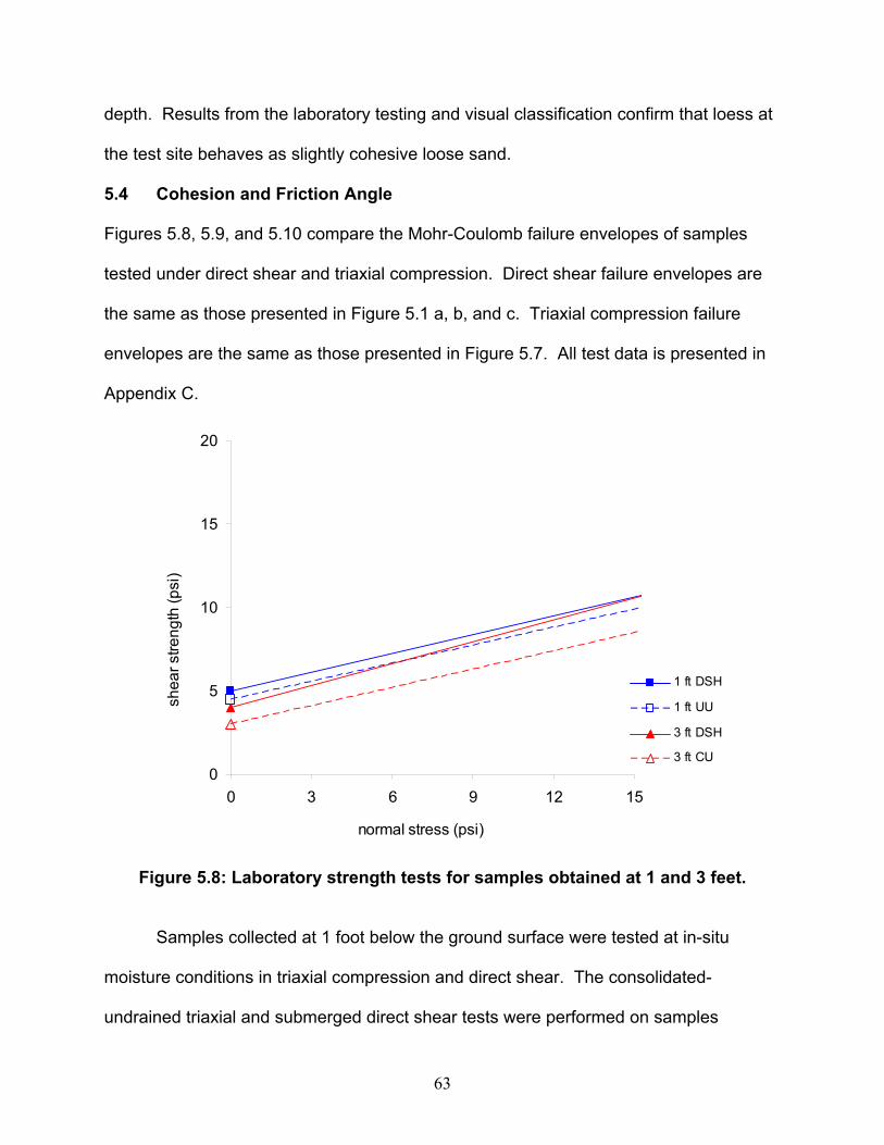
63
depth. Results from the laboratory testing and visual classification confirm that loess at
the test site behaves as slightly cohesive loose sand.
5.4 Cohesion and Friction Angle
Figures 5.8, 5.9, and 5.10 compare the Mohr-Coulomb failure envelopes of samples
tested under direct shear and triaxial compression. Direct shear failure envelopes are
the same as those presented in Figure 5.1 a, b, and c. Triaxial compression failure
envelopes are the same as those presented in Figure 5.7. All test data is presented in
Appendix C.
0
5
10
15
20
0 3 6 9 12 15
normal stress (psi)
shea
r stre
ngth
(psi
)
1 ft DSH
1 ft UU
3 ft DSH
3 ft CU
Figure 5.8: Laboratory strength tests for samples obtained at 1 and 3 feet.
Samples collected at 1 foot below the ground surface were tested at in-situ
moisture conditions in triaxial compression and direct shear. The consolidated-
undrained triaxial and submerged direct shear tests were performed on samples

64
collected at a 3 ft depth. Direct shear test results were similar to the triaxial compression
test results.
Soils sampled at 5 feet below the ground surface were tested at in-situ moisture
conditions. Soils sampled at 7 feet below the ground surface were subjected to
submerged direct shear and consolidated-undrained triaxial compression tests. Results
for all four tests were similar and consistent with previous results.
0
5
10
15
20
0 3 6 9 12 15
normal stress (psi)
shea
r stre
ngth
(psi
)
5 ft DSH
5 ft UU
7 ft DSH
7 ft CU
Figure 5.9: Laboratory strength tests for samples obtained at 5 and 7 feet.
Soils sampled at 15 feet below the ground surface were tested at in-situ moisture
conditions for both test types. Soils sampled at 25 feet below the ground surface were
tested in direct shear at in-situ moisture conditions and consolidated-undrained triaxial
compression. Samples from 25 feet had similar cohesive values. The friction angle
derived from the direct shear test was higher than from the triaxial test.
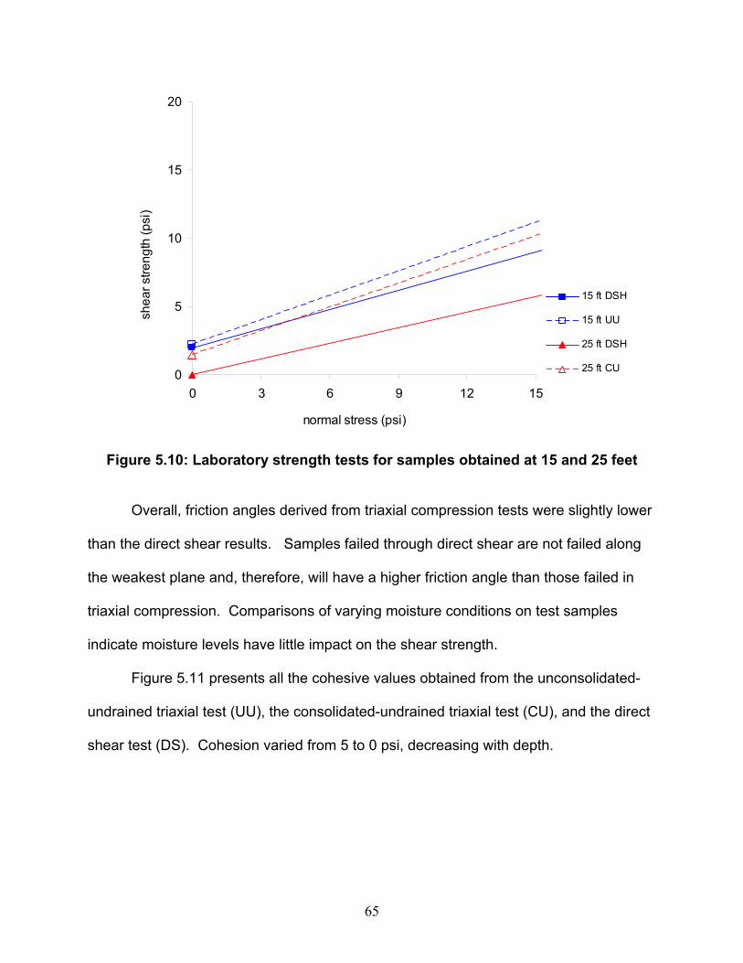
65
0
5
10
15
20
0 3 6 9 12 15
normal stress (psi)
shea
r stre
ngth
(psi
)
15 ft DSH
15 ft UU
25 ft DSH
25 ft CU
Figure 5.10: Laboratory strength tests for samples obtained at 15 and 25 feet
Overall, friction angles derived from triaxial compression tests were slightly lower
than the direct shear results. Samples failed through direct shear are not failed along
the weakest plane and, therefore, will have a higher friction angle than those failed in
triaxial compression. Comparisons of varying moisture conditions on test samples
indicate moisture levels have little impact on the shear strength.
Figure 5.11 presents all the cohesive values obtained from the unconsolidated-
undrained triaxial test (UU), the consolidated-undrained triaxial test (CU), and the direct
shear test (DS). Cohesion varied from 5 to 0 psi, decreasing with depth.
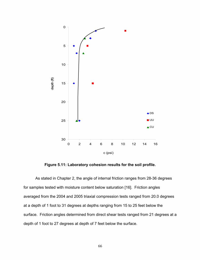
66
0
5
10
15
20
25
300 2 4 6 8 10 12 14 16
c (psi)
dept
h (ft
)
DS
UU
CU
Figure 5.11: Laboratory cohesion results for the soil profile.
As stated in Chapter 2, the angle of internal friction ranges from 28-36 degrees
for samples tested with moisture content below saturation [16]. Friction angles
averaged from the 2004 and 2005 triaxial compression tests ranged from 20.0 degrees
at a depth of 1 foot to 31 degrees at depths ranging from 15 to 25 feet below the
surface. Friction angles determined from direct shear tests ranged from 21 degrees at a
depth of 1 foot to 27 degrees at depth of 7 feet below the surface.
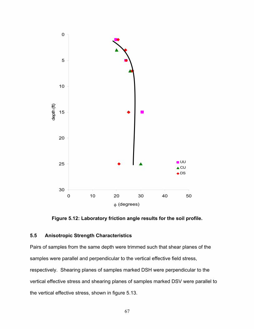
67
0
5
10
15
20
25
300 10 20 30 40 50
φ (degrees)
dept
h (ft
)
UUCUDS
Figure 5.12: Laboratory friction angle results for the soil profile.
5.5 Anisotropic Strength Characteristics
Pairs of samples from the same depth were trimmed such that shear planes of the
samples were parallel and perpendicular to the vertical effective field stress,
respectively. Shearing planes of samples marked DSH were perpendicular to the
vertical effective stress and shearing planes of samples marked DSV were parallel to
the vertical effective stress, shown in figure 5.13.
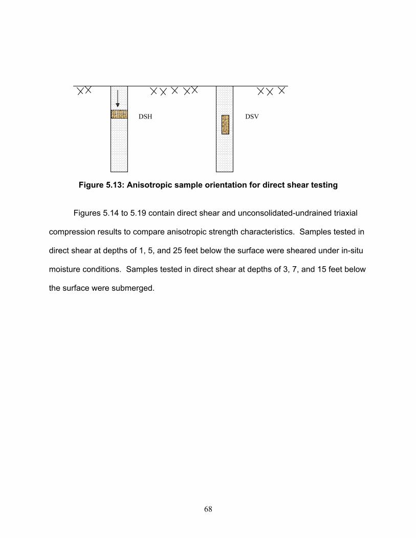
68
Figure 5.13: Anisotropic sample orientation for direct shear testing
Figures 5.14 to 5.19 contain direct shear and unconsolidated-undrained triaxial
compression results to compare anisotropic strength characteristics. Samples tested in
direct shear at depths of 1, 5, and 25 feet below the surface were sheared under in-situ
moisture conditions. Samples tested in direct shear at depths of 3, 7, and 15 feet below
the surface were submerged.
DSH DSV
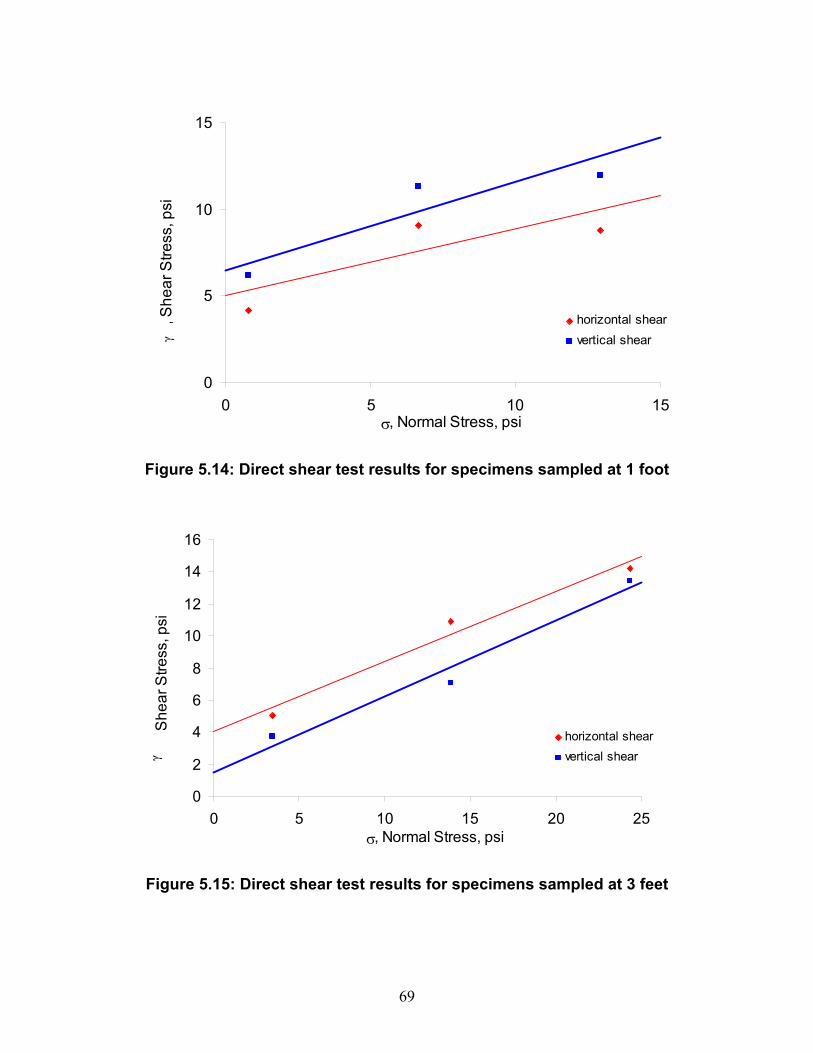
69
0
5
10
15
0 5 10 15σ, Normal Stress, psi
, She
ar S
tress
, psi
horizontal shearvertical shear
Figure 5.14: Direct shear test results for specimens sampled at 1 foot
0
2
4
6
8
10
12
14
16
0 5 10 15 20 25σ, Normal Stress, psi
, She
ar S
tress
, psi
horizontal shearvertical shear
Figure 5.15: Direct shear test results for specimens sampled at 3 feet
γ γ
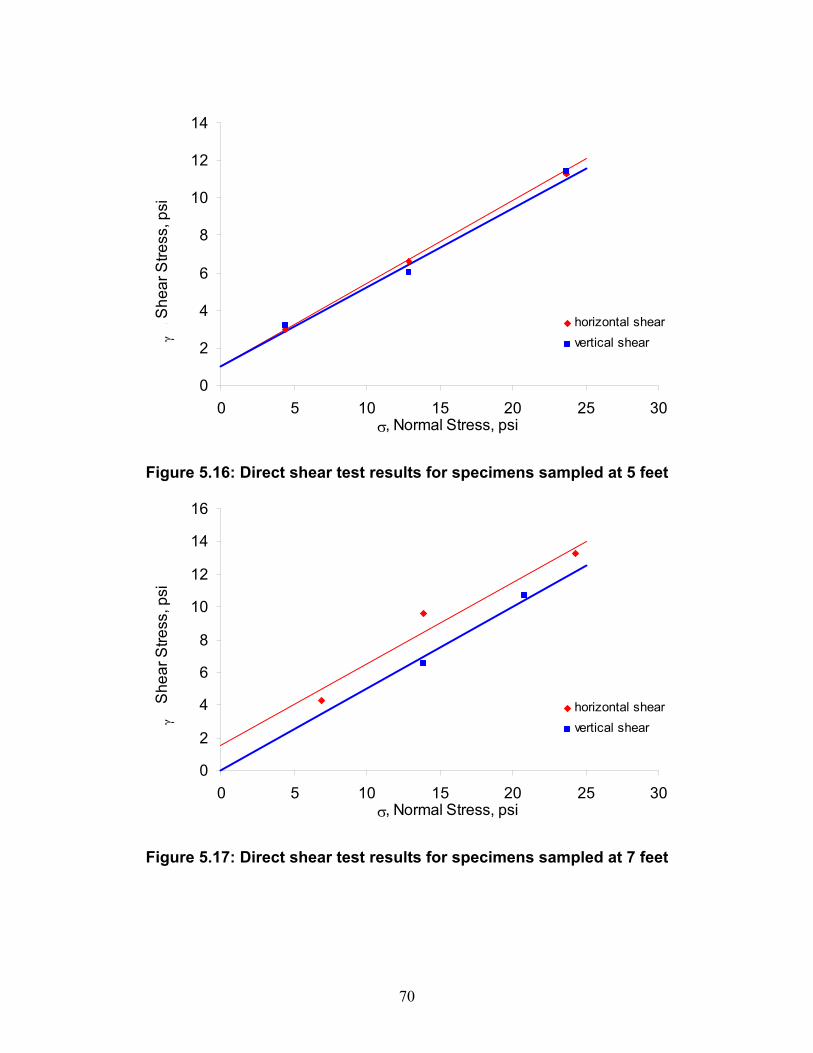
70
0
2
4
6
8
10
12
14
0 5 10 15 20 25 30σ, Normal Stress, psi
, She
ar S
tress
, psi
horizontal shearvertical shear
Figure 5.16: Direct shear test results for specimens sampled at 5 feet
0
2
4
6
8
10
12
14
16
0 5 10 15 20 25 30σ, Normal Stress, psi
, She
ar S
tress
, psi
horizontal shearvertical shear
Figure 5.17: Direct shear test results for specimens sampled at 7 feet
γ γ
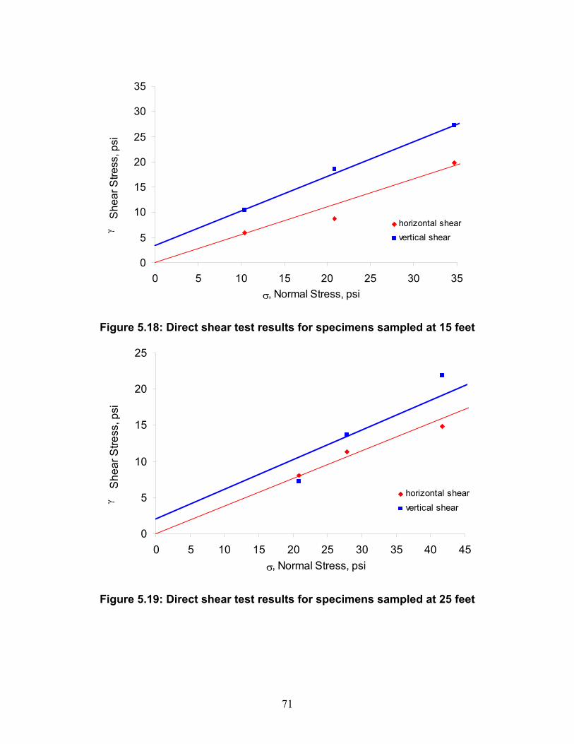
71
0
5
10
15
20
25
30
35
0 5 10 15 20 25 30 35σ, Normal Stress, psi
, She
ar S
tress
, psi
horizontal shearvertical shear
Figure 5.18: Direct shear test results for specimens sampled at 15 feet
0
5
10
15
20
25
0 5 10 15 20 25 30 35 40 45σ, Normal Stress, psi
, She
ar S
tress
, psi
horizontal shearvertical shear
Figure 5.19: Direct shear test results for specimens sampled at 25 feet
γ γ
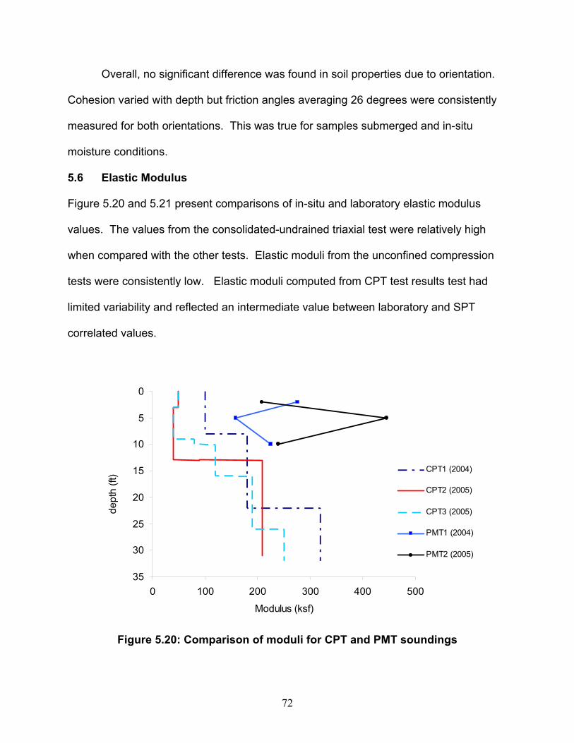
72
Overall, no significant difference was found in soil properties due to orientation.
Cohesion varied with depth but friction angles averaging 26 degrees were consistently
measured for both orientations. This was true for samples submerged and in-situ
moisture conditions.
5.6 Elastic Modulus
Figure 5.20 and 5.21 present comparisons of in-situ and laboratory elastic modulus
values. The values from the consolidated-undrained triaxial test were relatively high
when compared with the other tests. Elastic moduli from the unconfined compression
tests were consistently low. Elastic moduli computed from CPT test results test had
limited variability and reflected an intermediate value between laboratory and SPT
correlated values.
0
5
10
15
20
25
30
350 100 200 300 400 500
Modulus (ksf)
dept
h (ft
) CPT1 (2004)
CPT2 (2005)
CPT3 (2005)
PMT1 (2004)
PMT2 (2005)
Figure 5.20: Comparison of moduli for CPT and PMT soundings
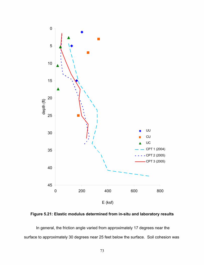
73
0
5
10
15
20
25
30
35
40
450 200 400 600 800
E (ksf)
dept
h (ft
)
UU
CU
UC
CPT 1 (2004)
CPT 2 (2005)
CPT 3 (2005)
Figure 5.21: Elastic modulus determined from in-situ and laboratory results
In general, the friction angle varied from approximately 17 degrees near the
surface to approximately 30 degrees near 25 feet below the surface. Soil cohesion was
74
at a maximum near the surface and decreased with depth to approximately 2 psi at 5
feet below the surface. The soil’s elastic modulus increased with depth and is
approximated best by CPT results. Moisture conditions and sample orientation had little
effect on the soil’s shear strength. All test results and soil properties analyzed indicate
loess at the test site behaved as a frictional soil with some cohesion.
75
Chapter 6
P-Y Analysis
KU did not have the capability to conduct full scale lateral load testing at the time of this
project. Therefore load testing and subsequent analysis was subcontracted to Dan
Brown and Associates. Dr. Steve Dapp conducted the testing and analysis with the
assistance of Dr. Brown. This chapter presents the equations developed by Drs. Dapp
and Brown to derive p-y curves specific to loess. A more detailed discussion by Drs.
Dapp and Brown is provided in Appendix D.
A hyperbolic model was developed to correlate ultimate soil resistance (Puo) to
the CPT cone tip resistance (qc) at any given depth below the surface. Cone values
were determined using an acoustic cone meeting the requirements of ASTM D 5778
and manufactured by Geotech AB of Sweeden. The ultimate soil resistance is
proportional to qc by a dimensionless correlation constant, Npo = 0.409.
cuo qP ⋅= 409.0 …………………………………………………………… 6.1
Where: Puo, and qc are in any consistent units of (force / length2)
The ultimate soil resistance is dependant only on the soil’s strength. It can be
made specific to a given pile (Pu) by multiplying by the diameter (b). Ultimate soil
resistance is now expressed as a unit length of the pile. This parameter is degraded for
a given load cycle (N) with the correlation constant of 0.24. The cyclic degradation term
in the denominator reduces to 1 for the initial cycle where N=1. In the case of a static
load, N=1.
76
)log(24.01 NbP
P uou ⋅+
⋅= ………………………………………....................6.2A
or
)log(24.01*409.0
NqcPu ⋅+
= ………………………………………....................6.2B
Where: b is in any consistent unit of (length),
N is dimensionless
Pu is in any consistent units of (force / length).
The second parameter needed is the reference displacement (Yi). The reference
displacement is the displacement at which the tangent to the p-y curve at zero
displacement (Ei) intersects the ultimate soil resistance asymptote (Pu). For lateral
displacement of the pile, this reference displacement (Yi) may be considered as
analogous to axial quake of a perfectly elastic-plastic bi-linear curve. It was determined
that the best fit to the load test data was obtained with the following reference
displacement (Yi).
Yi = 0.117 inches
Where Yi should be the displacement cited, and expressed in any consistent unit
of (length) corresponding to the other model parameters used.
The third parameter needed is the initial modulus (Ei), and is thus a simple
definitive expression of the ultimate soil resistance expressed on a per length of pile
basis (Pu), and the reference displacement (Yi).
i
ui Y
PE = ……………………………………………………………………6.3
Where: Pu is in any consistent units of (force / length).
Yi is in any consistent units of (length), and thus
Ei results in any consistent units of (force / length2).
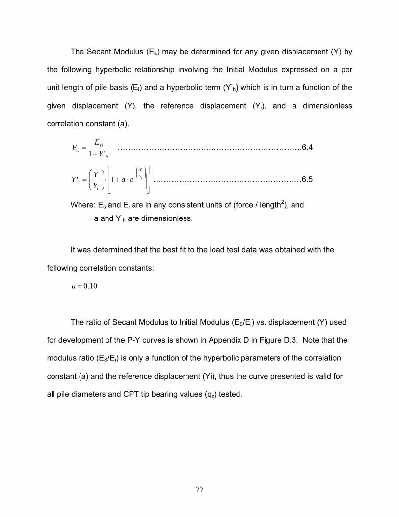
77
The Secant Modulus (Es) may be determined for any given displacement (Y) by
the following hyperbolic relationship involving the Initial Modulus expressed on a per
unit length of pile basis (Ei) and a hyperbolic term (Y’h) which is in turn a function of the
given displacement (Y), the reference displacement (Yi), and a dimensionless
correlation constant (a).
h
sis Y
EE
'1+= …………………………….……………………………….6.4
⎥⎥
⎦
⎤
⎢⎢
⎣
⎡⋅+⋅⎟⎟
⎠
⎞⎜⎜⎝
⎛=
⎟⎟⎠
⎞⎜⎜⎝
⎛−
iYY
ih ea
YYY 1' …………………………………………………6.5
Where: Es and Ei are in any consistent units of (force / length2), and
a and Y’h are dimensionless.
It was determined that the best fit to the load test data was obtained with the
following correlation constants:
10.0=a
The ratio of Secant Modulus to Initial Modulus (ES/Ei) vs. displacement (Y) used
for development of the P-Y curves is shown in Appendix D in Figure D.3. Note that the
modulus ratio (ES/Ei) is only a function of the hyperbolic parameters of the correlation
constant (a) and the reference displacement (Yi), thus the curve presented is valid for
all pile diameters and CPT tip bearing values (qc) tested.
78
Chapter 7
Conclusion and Recommendations
7.1 Soil Classification
Soil classification parameters were determined from laboratory and in-situ methods.
Laboratory analyses included all index property testing and in-situ classification was
determined by three CPT analyses. Laboratory index property results are presented on
grain-size distribution curves in Appendix C, section 4. The soil was classified as low
plasticity clay from the surface to a depth of 16 feet, low plasticity silt from depths of 16-
28 feet, and low plasticity clay from depths of 28-32 feet, where borings were
terminated.
Three computerized CPT profiles were generated and are presented in Appendix
C, section 6. In general, the profiles consisted of alternating layers of clay, sand, silty
sand, and sandy silt. As shown in Figure 3.7, CPT 1 and CPT 2 were located near
drilled shaft 6 in 2004 and 2005, respectively. CPT 3 was located between shaft 1 and
2 in 2005. Computerized results from CPT 1 and 3 were similar, while results for CPT 2
included five layers of gravely sand. The results were inconsistent. Therefore,
computerized CPT results in loess are not reliable and should be viewed with caution.
Correlations derived from Robertson & Campanella [28] generally classify the soil
as sand, silty sand, and sandy silt. It did not account for the cohesive nature of the
loess. From the literature review, the greatest amount of clay should be found near the
surface and the largest amount of sand should be located near the bottom of Loveland

79
members. Therefore, the most accurate soil classification was derived from laboratory
index property tests.
7.2 Collapse
As stated in the literature review, loess is well known for its collapsibility. Large
settlements associated with collapse are an important physical and structural property
of loess. Soils with montmorillonite as the cementing material tend to swell with an
increase in moisture and create a potential for the soil matrix to collapse. Plasticity
indices are an indication of the amount of clay present in the soil. A high value
corresponds to high percentages of montmorillonite in the soil. Dry unit weight is also
an indicator of the soil’s collapsibility. With an increase in moisture, settlement will be
small for soils with dry unit weights exceeding 90 pcf. Soils with moisture contents
between 10 to 15 percent have moderately high strength and a small amount of
settlement [7]. Therefore, soils with high field densities, low moisture contents, and clay
cementation can be expected to have a low collapse potential.
Soil at the test sight was subjected to collapse tests at 1 and 25 feet below the
surface. At these depths, the soil had the highest void ratio and would suffer the largest
settlement due to an increase in moisture. Loess samples tested had an average dry
unit weight of 90 pcf, a plastic index and moisture content of 13 and 20% at 1 foot and
were non-plastic with a moisture content of 10% at 25 feet. At both depths, the test
sight had low plastic index values, moderate to low moisture contents, and high dry unit
weights. As expected, the test sight was found to be slightly collapsible. If a soil is not
tested directly for its collapse potential, a combination of dry unit weight, moisture
80
content, and the plastic index are good parameters for approximating collapse
susceptibility.
7.3 Anisotropy
Strength parameters were used to determine soil anisotropy. As presented in Figure
5.12, pairs of samples from the same depth were trimmed such that shear planes of the
samples were parallel and perpendicular to the vertical effective field stress,
respectively. There was some variability in cohesion due to varying moisture
conditions. For each depth friction angles were consistent regardless of test orientation.
Overall, no significant difference was found in soil properties due to orientation.
7.4 Soil Modulus Values
Soil modulus of elasticity (Em) is a measure of the stiffness of the soil and can be
calculated from laboratory and in-situ test data. Figure 5.17 presents a comparison of
the soil’s elastic modulus derived from unconsolidated-undrained, consolidated-
undrained, unconfined compression, and CPT tests. The average values for the
modulus of elasticity were consistent among the tests. However, laboratory tests
calculated higher Em values near the surface and decreased with depth. The three CPT
tests developed lower Em values near the surface and continued to increase with depth.
When compared to all the tests, unconfined compression results developed into the
lowest values of Em and consolidated-undrained test results were the highest values.
Overall, the three CPT tests provided a representative and continuous profile of Em
results and the test is recommended for estimation of elastic modulus. The CPT results
were used as the basis for the p-y curve analysis.
81
7.5 Strength Parameters
Total and effective shear strength parameters were determined from direct shear and
triaxial compression tests. Overall, friction angles derived from triaxial compression
tests were slightly lower than the direct shear results. Reese and Matlock recommend
using triaxial compression tests, with confining pressure equal to the overburden
pressure, for determining the shear strength of sand above and below the water table.
They state the strength values may be conservative but would be more representative
than other tests [19]. Matlock recommended in-situ vane-shear tests and
unconsolidated-undrained triaxial compression tests for soft clays below the water table.
For the loess at the test site (which was far above the groundwater table),
unconsolidated-undrained total strength parameters and consolidated-undrained
effective strength parameters were similar and more conservative than the direct shear
results. As determined in Chapter 5, loess behaves more like loose sand than a
cohesive material. Therefore, triaxial compression testing is recommended to
determine strength parameters, with test conditions dependent on soil profile.
7.6 In-Situ Moisture Conditions
Moisture conditions in 2004 and 2005 are plotted on boring logs L and M, respectively,
in Appendix B. From the surface to an approximate depth of 12 feet, moisture contents
ranged from 20-25 %. From an approximate depth of 12-26 feet below the surface,
moisture contents decreased with depth from 20-10 % in 2004. Moisture conditions in
2005 were similar. From the surface to an approximate depth of 10 feet, moisture
contents ranged from 20-23 %. From an approximate depth of 10-32 feet below the
surface, moisture contents decreased with depth from 20-10 %.
82
A comparable amount of rainfall occurred during sampling in 2004 and the day
before sampling in 2005. In-situ moisture conditions in 2005 were slightly drier than
2004; however, no substantial difference occurred in any test result due to the small
moisture difference.
7.7 Correlation for P-Y Curves
As discussed in Chapter 5 and sections 7.1 to 7.6, the Loveland loess tested and
analyzed behaved as loose sand with slight cohesion. This confirms Frantzen and
Clowers statement that “in the case of static loading, p-y curves developed for sand
may be used to predict lateral load response of piles embedded in dry loess [3].”
Dan Brown and Associates developed a hyperbolic model specific to p-y curves
in loess. The equations were presented in Chapter 6 and detailed in Appendix D. The
hyperbolic model was developed to provide the secant modulus of the p-y curve at any
given displacement.
7.8 Additional Research
Future laboratory testing could include analyzing results from consolidated-drained and
consolidated-undrained triaxial compression tests on loess samples that are more
susceptible to collapse.
83
References:
[1] Coduto, Donald P., Foundation design, Prentice-Hall, Inc., Upper Saddle River,
New Jersey, 1999.
[2] COM624P (1993), “Laterally Loaded Pile Analysis Program for the
Microcomputer,” FHWA-SA-91-048, computer program documentation by Wang,
S.T. and Reese, L.C. 487 pp 487.
[3] Clowers, Karen A. and Frantzen, Jeffrey A., “Response of Piles in Loess to
Lateral Loads,” Research Report No. FHWA-KS-92-4, Kansas Department of
Transportation, Division of Operations Bureau of Materials and Research,
November, 1992.
[4] Marosi, Paul, “A Review of the Evolution of Theories on the Origin of Loess,”
Loess, Lithology and Genesis, Ian J. Smalley; Ed., Dowden, Hutchinson, & Ross,
Inc., Distributed by Halsted Press, 1975, pp. 402-414.
[5] Terzaghi, Karl, Peck, Ralph B., and Mesri, Gholamreza, Soil Mechanics in
Engineering Practice, third ed., John Wiley & Sons, Inc., New York,NY, 1996.
[6] Bandyopadhyay, S.S., “Geotechnical Evaluation of Loessial Soils in Kansas,”
Transportation Research Record 945.
[7] Gibbs, H.J. and Holland, W.Y., “Petrographic and Engineering Properties of
Loess”, Engineer Monograph No. 28, U.S. Bureau of Reclamation, Denver, CO,
1960.
[8] Crumpton, Carl F. and Badgley, William S., “A Study of the Clay Mineralogy of
Loess in Kansas in Relation to its Engineering Properties,” U.S. Department of
Commerce Bureau of Public Roads, 1965.
[9] Swineford, A. and Frye, J.C., “Petrography of the Peoria Loess in Kansas,”
Journal of Geology, Vol. 59, No. 4, 1951, pp. 306-322.
[10] Beavers, A.H., “Source and Deposition of Clay Minerals in Peorian Loess,”
Loess, Lithology and Genesis; Ian J. Smalley; Ed., Dowden, Hutchinson, & Ross,
Inc., Distributed by Halsted Press; 1975, pp. 149.
[11] Smalley, Ian J., “Introduction,” Loess, Lithology and Genesis; Ian J. Smalley; Ed.,
Dowden, Hutchinson, & Ross, Inc., Distributed by Halsted Press; 1975, pp. 1-9.
84
[12] Swinford, Ada and Frye, John C., “Petrographic Comparison of Some Loess
Samples from Western Europe with Kansas Loess,” Loess, Lithology and
Genesis, Ian J. Smalley; Ed., Dowden, Hutchinson, & Ross, Inc., Distributed by
Halsted Press, 1975, pp.183.
[13] Zeller, Doris E., The Stratigraphic Succession in Kansas, State Geological
Survey of Kansas, Bulletin 189.
[14] Howe, Wallace B., The Stratigraphic Succession in Missouri, John W. Koenig;
Ed., State Geological Survey of Missouri, Vol. XL, second series, September
1961.
[15] Paliwal, K.V., Hobbs, J.A., Bidwell, O.H., and R. Ellis, Jr., “Mineralogical and
Chemical Characteristics of Four Western Kansas Soils,” Transactions of the
Kansas Academy of Science, Vol. 67, Issue 4, 1965, pp. 617-629.
[16] Sheeler, J.B., “Summarization and Comparison of Engineering Properties of
Loess in the United States,” Record No. 212, Highway Research Board,
Washington, DC 1968, pp 1-9.
[17] Coduto, Donald P., Geotechnical Engineering, Principles and Practices, Prentice-
Hall, Inc., Upper Saddle River, New Jersey, 1999.
[18] Ashour, Mohamed and Norris, G., “Modeling Lateral Soil-Pile Response Based
on Soil-Pile Interaction,” Journal of Geotechnical and Geoenvironmental
Engineering, Vol. 126, No. 5, May 2000.
[19] Welch, Robert C. and Reese, Lymon C., “Lateral Load Behavior of Drilled
Shafts,” Research Report 89-10, Project 3-5-65-89, Center for Highway
Research, the University of Texas at Austin, May 1972.
[20] Mokwa, Robert L., Duncan, Michael, and Helmers, Matthew J., “Development of
p-y Curves for Partly Saturated Silts and Clays,” Geotechnical Special
Publication, ASCE, NO. 100, 2000, pp 224-239.
[21] McClelland, Bramlette and Focht, John A., Jr., “Soil Modulus for Laterally Loaded
Piles,” Journal of the Proceedings of the American Society of Civil Engineers,
Soil Mechanics and Foundations Division, Proceeding Paper 1081.
85
[22] Anderson, J.B., Townsend, F.C., and Grajales, B., “Case History Evaluation of
Laterally Loaded Piles,” Journal of Geotechnical and Geoenvironmental
Engineering, ASCE, March 2003, #187.
[23] Duncan, Michael J., Evans, Leonard T. Jr., and Ooi, Phillip S. K., “Lateral Load
Analysis of Single Piles and Drilled Shafts,” Journal of Geotechnical Engineering,
Copyright ASCE, vol. 120 NO. 6, 1994, pp 1018.
[24] Lamb, R.O., “Geotechnical Aspects of Leaching of Carbonates from Loessial
Soils,” Physico-Chemical Aspects of Soil and Related Materials, ASTM STP
1095, “K.B. Hoddinott and R.O. Lamb, Eds., American Society for Testing and
Materials, Philadelphia, 1990, pp. 29-43.
[25] ASTM International, West Conshohocken, PA.
[26] Bishop and Henkel, The Measurement of Soil Properties in the Triaxial Test, 2nd
ed, Edward Arnold (Publishers) Ltd., London W1X 8LL.
[27] Peck, R.B., Hanson, W.E., and Thornburn, T.H., Foundation Engineering, Wiley,
New York, 1974.
[28] Robertson, P.K. and Campanella, R.G., Interpretation of cone penetration tests -
Part I: Sand. Can. Geotech. Journ., 20:718-733.
[29] Robertson, P.K., Campanella, R.G., and Wightman, A., SPT-CPT correlations.
Technical report, Soil Mech. Series No. 62, Dept. of Civil Engnrg., Univ. of British
Columbia.
[30] Schmertmann, J.H., “Measurement of In-situ Shear Strength,” Journal of the
Proceedings of the American Society of Civil Engineers, June 1-4, 1975, vol. II.
[31] Wolff, Thomas F, “Geotechnical Judgment in Foundation Design.” Foundation
Engineering: Current Principles and Practice, Vol. 2, ASCE Evanston, IL, June
25-29, 1989, ASCE, New York, NY, pp 903-917.
[32] Kulhawy, F.H., Mayne, P.W., “Relative density, SPT and CPT interrelationships,”
Proc Int Symp Calibration Chamber Test, 1992.
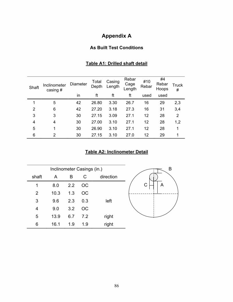
86
Appendix A
As Built Test Conditions
Table A1: Drilled shaft detail
Diameter Total Depth
Casing Length
Rebar Cage
Length
#10 Rebar
#4 Rebar Hoops Shaft Inclinometer
casing # in ft ft ft used used
Truck #
1 5 42 26.80 3.30 26.7 16 29 2,3 2 6 42 27.20 3.18 27.3 16 31 3,4 3 3 30 27.15 3.09 27.1 12 28 2 4 4 30 27.00 3.10 27.1 12 28 1,2 5 1 30 26.90 3.10 27.1 12 28 1 6 2 30 27.15 3.10 27.0 12 29 1
Table A2: Inclinometer Detail
Inclinometer Casings (in.)
shaft A B C direction
1 8.0 2.2 OC
2 10.3 1.3 OC
3 9.6 2.3 0.3 left
4 9.0 3.2 OC
5 13.9 6.7 7.2 right
6 16.1 1.9 1.9 right
A C
B
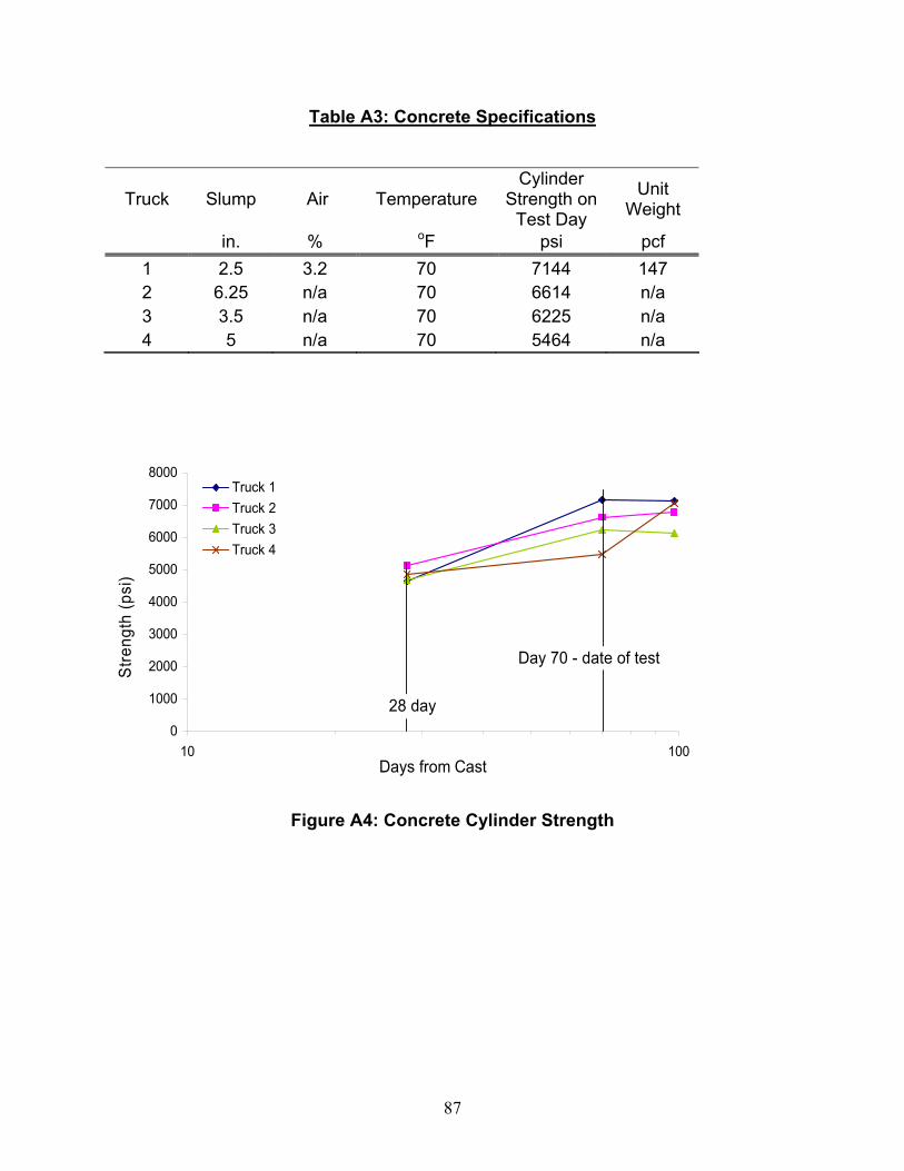
87
Table A3: Concrete Specifications
Truck Slump Air Temperature Cylinder
Strength on Test Day
Unit Weight
in. % oF psi pcf 1 2.5 3.2 70 7144 147 2 6.25 n/a 70 6614 n/a 3 3.5 n/a 70 6225 n/a 4 5 n/a 70 5464 n/a
0
1000
2000
3000
4000
5000
6000
7000
8000
10 100Days from Cast
Stre
ngth
(psi
)
Truck 1Truck 2Truck 3Truck 4
Day 70 - date of test
28 day
Figure A4: Concrete Cylinder Strength
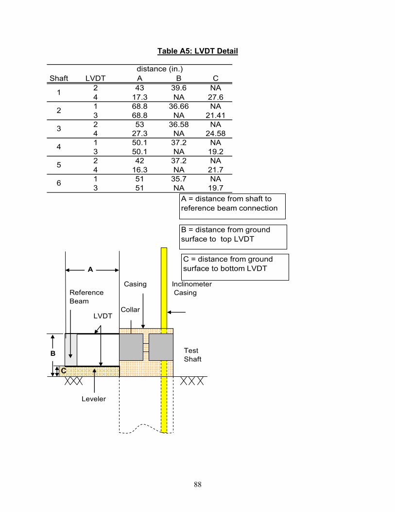
88
Table A5: LVDT Detail
Shaft LVDT A B C2 43 39.6 NA4 17.3 NA 27.61 68.8 36.66 NA3 68.8 NA 21.412 53 36.58 NA4 27.3 NA 24.581 50.1 37.2 NA3 50.1 NA 19.22 42 37.2 NA4 16.3 NA 21.71 51 35.7 NA3 51 NA 19.7
distance (in.)
5
6
1
2
3
4
Inclinometer Casing
Test Shaft
Collar
Casing
LVDT
Reference Beam
Leveler
A
B
B = distance from ground surface to top LVDT
A = distance from shaft to reference beam connection
C
C = distance from ground surface to bottom LVDT
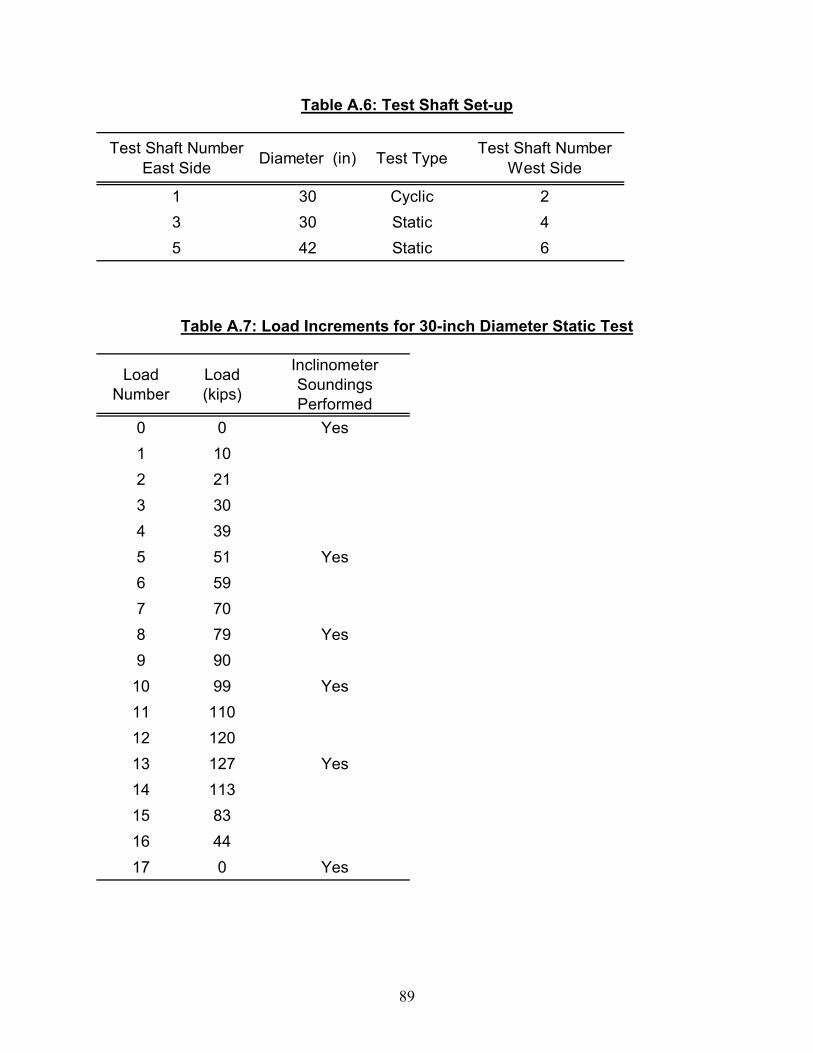
89
Table A.6: Test Shaft Set-up
Test Shaft Number East Side Diameter (in) Test Type Test Shaft Number
West Side
1 30 Cyclic 23 30 Static 45 42 Static 6
Table A.7: Load Increments for 30-inch Diameter Static Test
Load Number
Load (kips)
Inclinometer Soundings Performed
0 0 Yes1 102 213 304 395 51 Yes6 597 708 79 Yes9 90
10 99 Yes11 11012 12013 127 Yes14 11315 8316 4417 0 Yes
90
Table A.8: Load Increments for the 42-inch Diameter Static Test
Load Number
Load (kips)
Inclinometer Soundings Performed
0 0 Yes1 182 333 494 625 786 927 107 Yes8 1239 137
10 150 Yes11 16812 18313 193 Yes14 21415 219 Yes16 16517 11318 6019 0 Yes
Table A.9: Load Increments for the 30-inch Diameter Cyclic Test
Load Increment Load Cycles
Deflect ReturnN/A None 0 0A 1 through 10 50 -15B 1 through 10 79 -25C 1 through 10 99 -30D 1 through 10 127 -30
Inclinometer Soundings
Approximate Load (kips)
Prior to Loading
at Load Cycles 1 and 10 for each Load Increment
91
Appendix B
Boring Logs

92
93
94
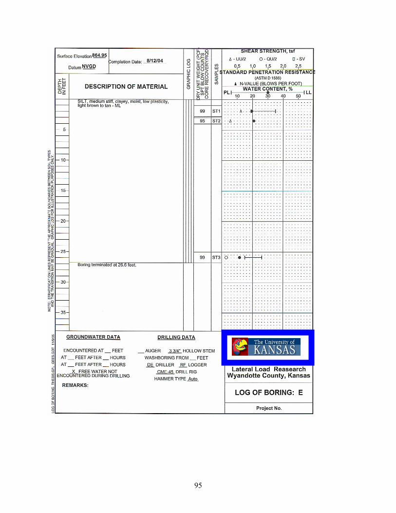
95
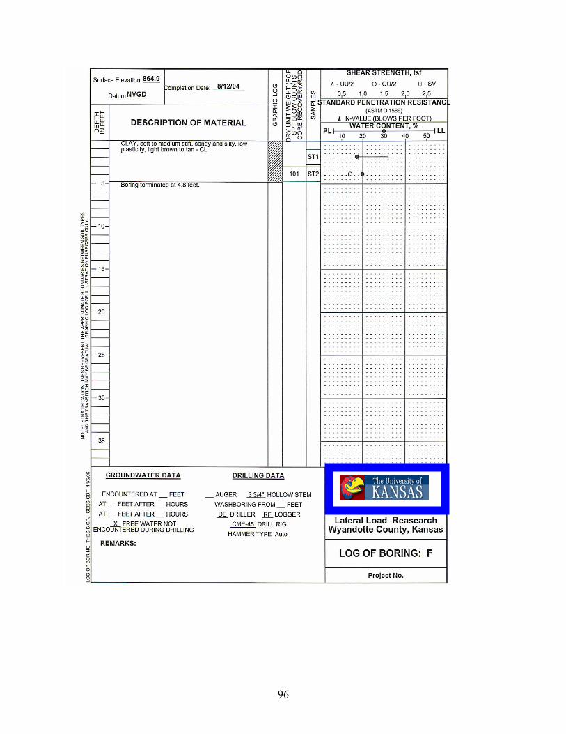
96

97
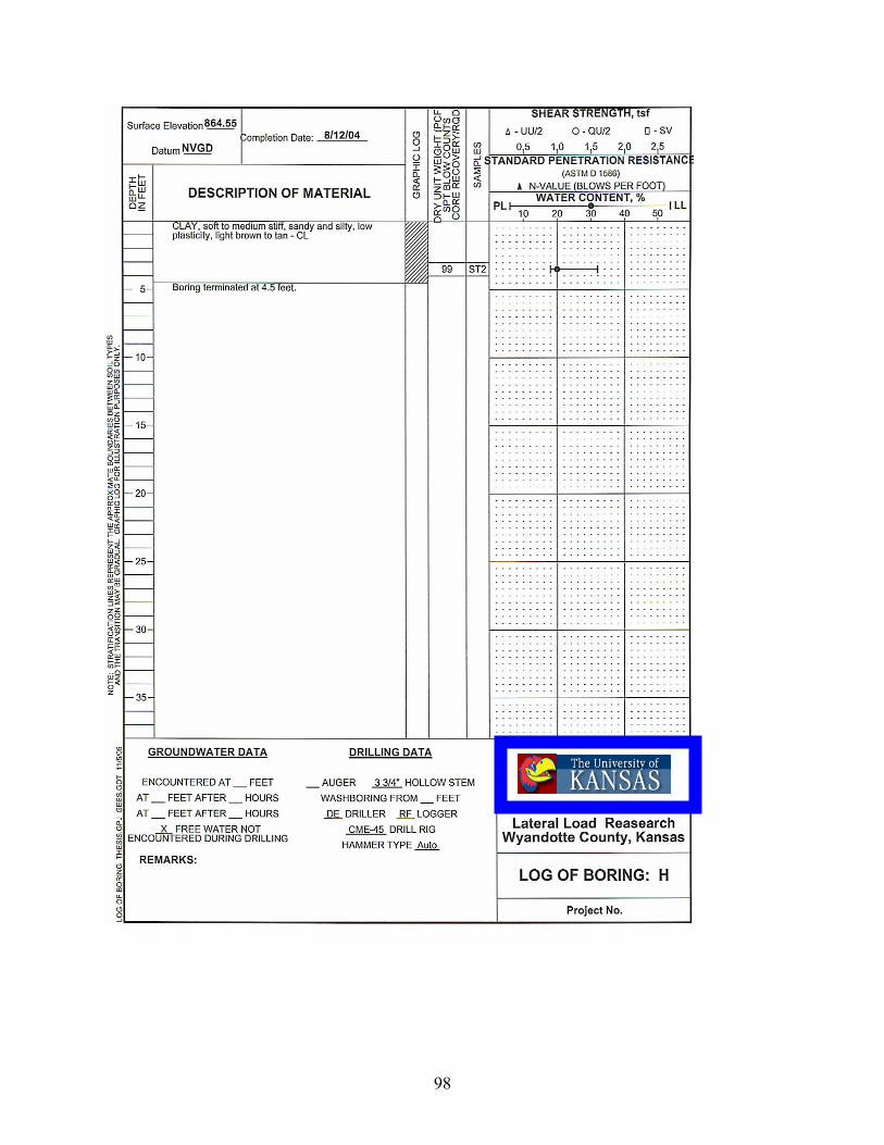
98
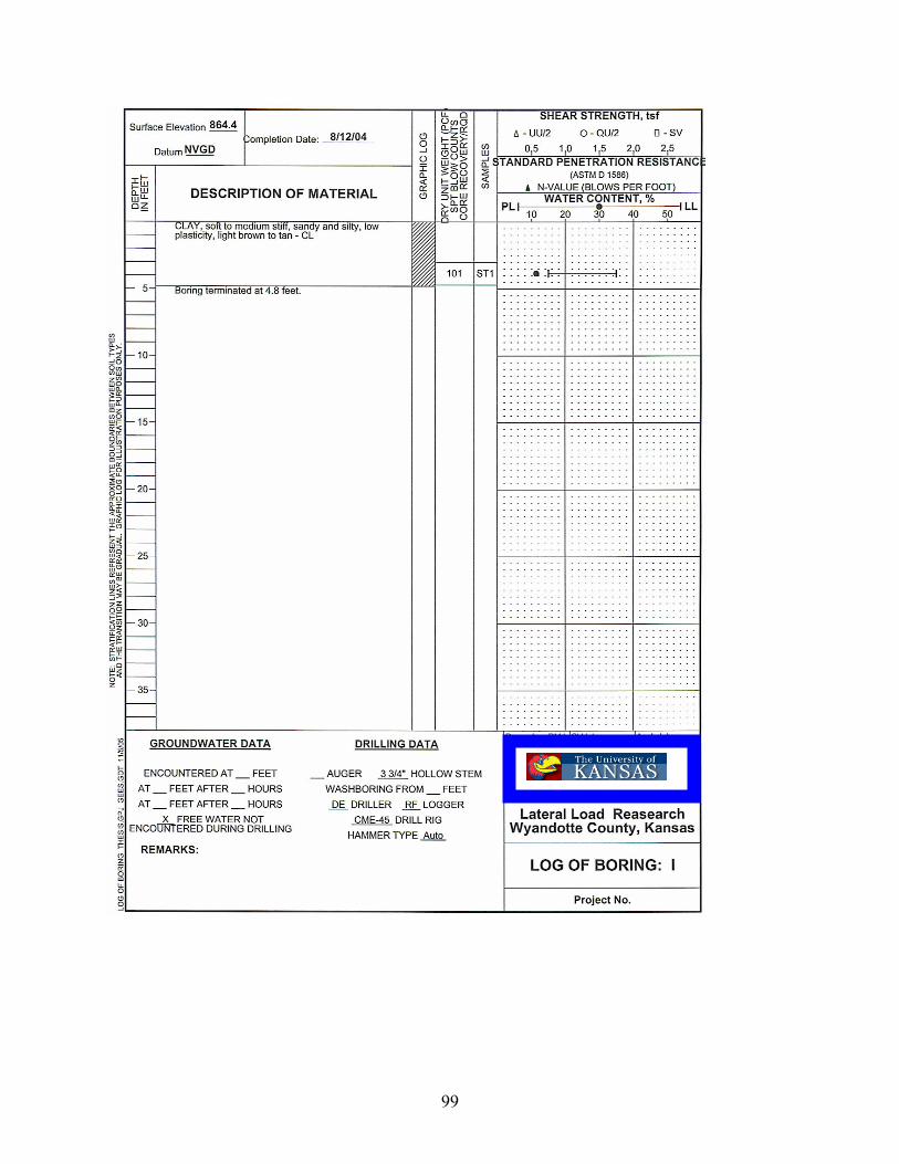
99

100

101
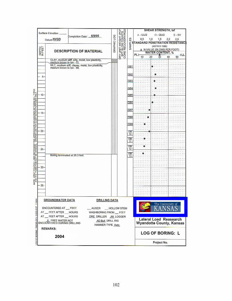
102
2004

103
2005
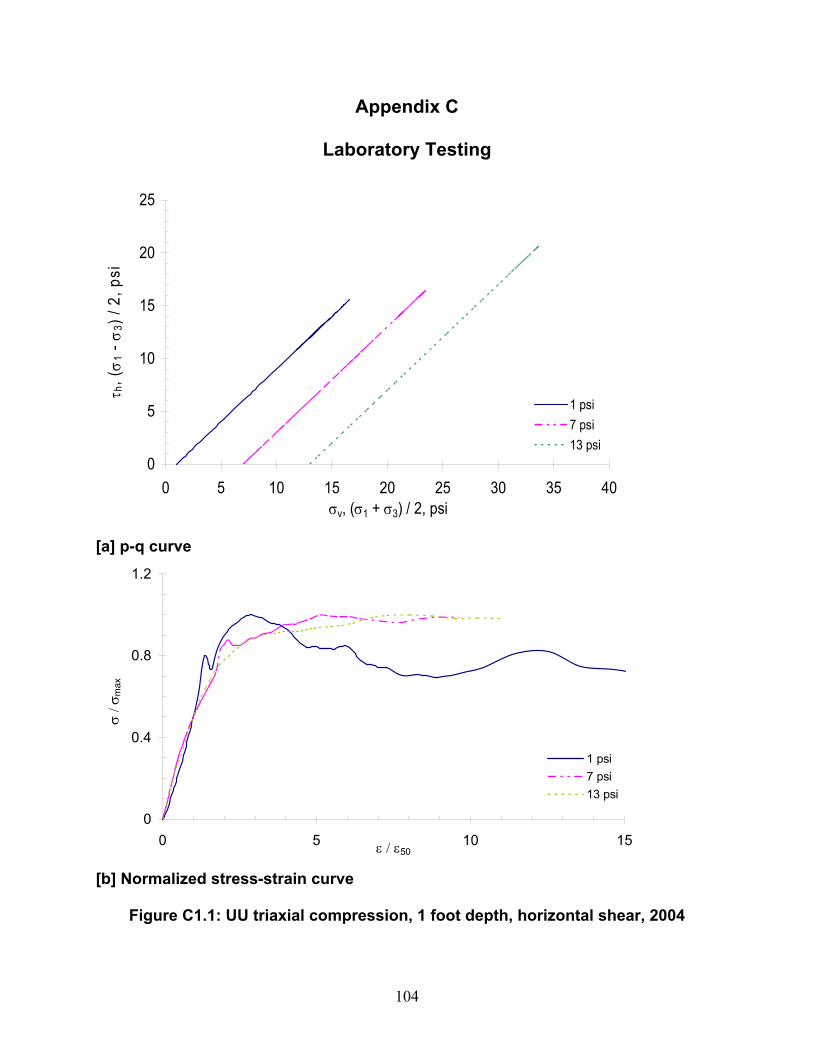
104
Appendix C
Laboratory Testing
0
5
10
15
20
25
0 5 10 15 20 25 30 35 40σv, (σ1 + σ3) / 2, psi
τ h, (
σ 1 -
σ 3) /
2, p
si
1 psi7 psi13 psi
[a] p-q curve
0
0.4
0.8
1.2
0 5 10 15ε / ε50
σ / σ
max
1 psi7 psi13 psi
[b] Normalized stress-strain curve
Figure C1.1: UU triaxial compression, 1 foot depth, horizontal shear, 2004
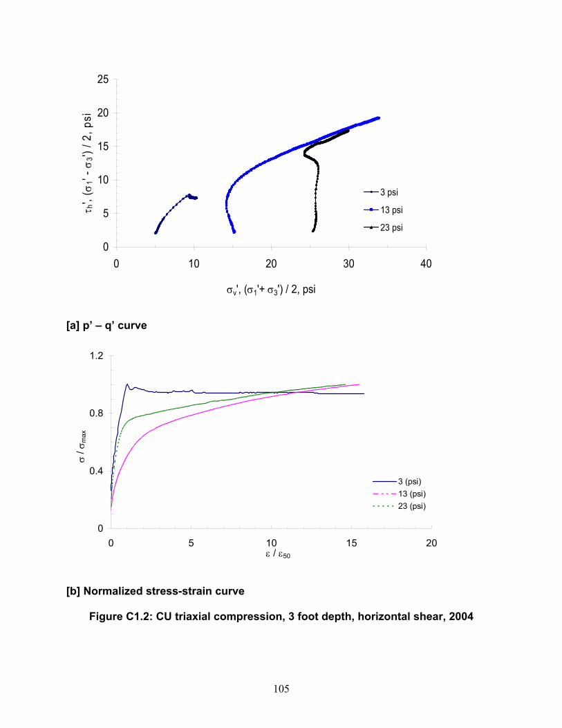
105
0
5
10
15
20
25
0 10 20 30 40
σv', (σ1'+ σ3') / 2, psi
τ h',
( σ1'
- σ3')
/ 2,
psi
3 psi
13 psi
23 psi
[a] p’ – q’ curve
0
0.4
0.8
1.2
0 5 10 15 20ε / ε50
σ / σ
max
3 (psi)13 (psi)23 (psi)
[b] Normalized stress-strain curve
Figure C1.2: CU triaxial compression, 3 foot depth, horizontal shear, 2004
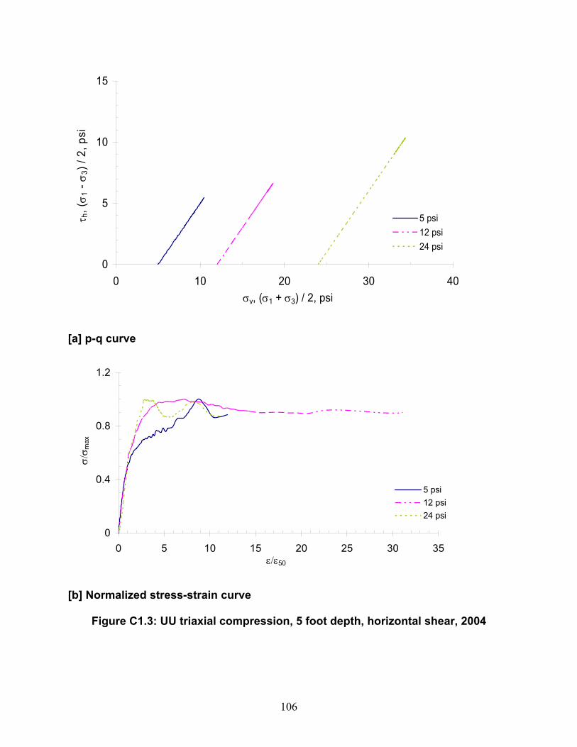
106
0
5
10
15
0 10 20 30 40σv, (σ1 + σ3) / 2, psi
τ h, (
σ 1 -
σ 3) /
2, p
si
5 psi12 psi24 psi
[a] p-q curve
0
0.4
0.8
1.2
0 5 10 15 20 25 30 35ε/ε50
σ/σ m
ax
5 psi12 psi24 psi
[b] Normalized stress-strain curve
Figure C1.3: UU triaxial compression, 5 foot depth, horizontal shear, 2004
107
0
5
10
15
0 5 10 15 20 25 30σv', (σ1' + σ3') / 2, psi
τ h',
( σ1'
- σ3')
/ 2,
psi
6 psi14 psi26 psi
[a] p’ - q’ curve
0
0.4
0.8
1.2
0 20 40 60 80 100 120ε / ε50
σ / σ
max
6 (psi)14 (psi)26 (psi)
[b] Normalized stress - strain curve
Figure C1.4: CU triaxial compression, 7 foot depth, horizontal shear, 2004
108
0
5
10
15
0 5 10 15 20 25 30 35 40 45
σv, (σ1 + σ3) / 2, psi
τ h, (
σ 1 -
σ 3) /
2, p
si
12 psi32 psi
[a] p - q curve
0
0.4
0.8
1.2
0 5 10 15 20 25 30ε / ε50
σ / σ
max
12 (psi)32 (psi)
[b] Normalized stress – strain curve
Figure C1.5: UU triaxial compression, 15 foot depth, horizontal shear, 2004
109
0
10
20
30
40
0 10 20 30 40 50 60 70 80σv', (σ1' + σ3') / 2, psi
τ h',
( σ1'
- σ3')
/ 2,
psi
20 psi28 psi40 psi
[a] p’- q’ curve
0
0.4
0.8
1.2
0 5 10 15 20
ε / ε50
σ / σ
max
20 (psi)28 (psi)40 (psi)
[b] Normalized stress-strain curve
Figure C1.6: CU triaxial compression, 25 foot depth, horizontal shear, 2004

110
0
5
10
15
20
25
0 5 10 15 20 25 30 35 40σv, (σ1 + σ3) / 2, psi
τ h, (
σ 1 -
σ 3) /
2, p
si
1psi7psi13psi
`
[a] p – q curve
0
0.4
0.8
1.2
0 5 10ε / ε50
σ / σ
max
1 psi7 psi13 psi
[b] Normalized stress – strain curve
Figure C1.7: UU triaxial compression, 1 foot depth, horizontal shear, 2005
111
0
5
10
15
0 5 10 15 20 25 30 35 40 45
σv, (σ1 + σ3) / 2, psi
τ h, (
σ 1 -
σ 3) /
2, p
si
4psi12psi24psi
[a] p – q curve
0
0.4
0.8
1.2
0 5 10ε / ε50
σ / σ
max
4 psi12 psi24 psi
[b] Normalized stress – strain curve
Figure C1.8: UU triaxial compression, 5 foot depth, horizontal shear, 2005
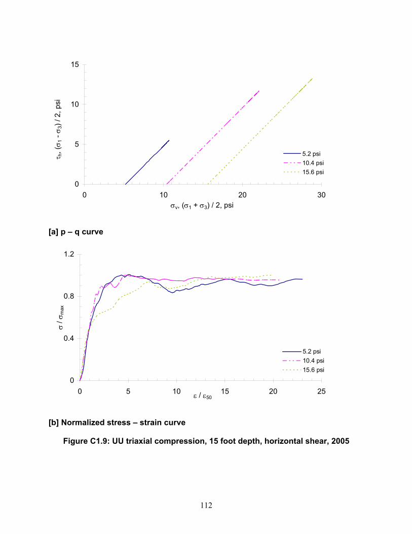
112
0
5
10
15
0 10 20 30σv, (σ1 + σ3) / 2, psi
τ h, (
σ 1 -
σ 3) /
2, p
si
5.2 psi10.4 psi15.6 psi
[a] p – q curve
0
0.4
0.8
1.2
0 5 10 15 20 25ε / ε50
σ / σ
max
5.2 psi10.4 psi15.6 psi
[b] Normalized stress – strain curve
Figure C1.9: UU triaxial compression, 15 foot depth, horizontal shear, 2005

113
0
2
4
6
8
10
12
14
0 0.05 0.1 0.15Strain, in/in
Stre
ss, p
si
0.793231797 psi6.650943532 psi12.92133919 psi
0.8 psi6.7 psi
13 psi
[a] Vertical Shear
0
2
4
6
8
10
0 0.02 0.04 0.06 0.08
Strain, in/in
Stre
ss, p
si
0.785909658 psi6.650943532 psi12.9154408 psi
0.8 psi6.7 psi13 psi
[b] Horizontal Shear
Figure C2.1: Direct Shear, 1 foot depth, 2004
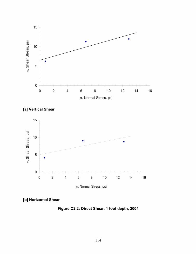
114
0
5
10
15
0 2 4 6 8 10 12 14 16
σ, Normal Stress, psi
τ, S
hear
Stre
ss, p
si
[a] Vertical Shear
0
5
10
15
0 2 4 6 8 10 12 14 16
σ, Normal Stress, psi
τ, S
hear
Stre
ss, p
si
[b] Horizontal Shear
Figure C2.2: Direct Shear, 1 foot depth, 2004

115
0
2
4
6
8
10
12
14
16
0.00 0.06 0.12 0.18Strain, in/in
Stre
ss, p
si
3.5 psi14 psi24.5 psi
[a] Vertical Shear
0
2
4
6
8
10
12
14
16
0.00 0.06 0.12 0.18Strain, in/in
Stre
ss, p
si
3.5 psi14 psi24.5 psi
[b] Horizontal Shear
Figure C2.3: Direct Shear, 3 foot depth, 2004

116
0
5
10
15
0 5 10 15 20 25σ, Normal Stress, psi
τ, S
hear
Stre
ss, p
si
[a] Vertical Shear
0
5
10
15
0 5 10 15 20 25σ, Normal Stress, psi
τ, S
hear
Stre
ss, p
si
[b] Horizontal Shear
Figure C2.4: Direct Shear, 3 foot depth, 2004
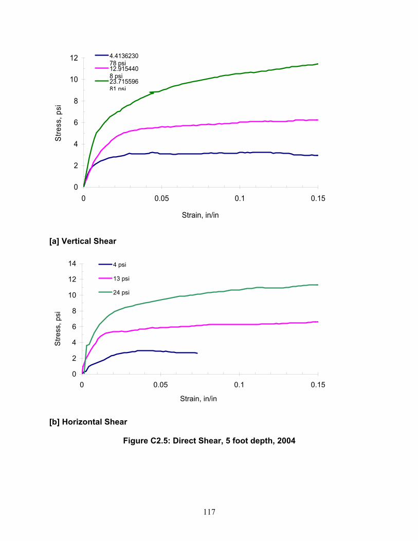
117
0
2
4
6
8
10
12
0 0.05 0.1 0.15
Strain, in/in
Stre
ss, p
si4.413623078 psi12.9154408 psi23.71559681 psi
[a] Vertical Shear
0
2
4
6
8
10
12
14
0 0.05 0.1 0.15
Strain, in/in
Stre
ss, p
si
4 psi
13 psi
24 psi
[b] Horizontal Shear
Figure C2.5: Direct Shear, 5 foot depth, 2004
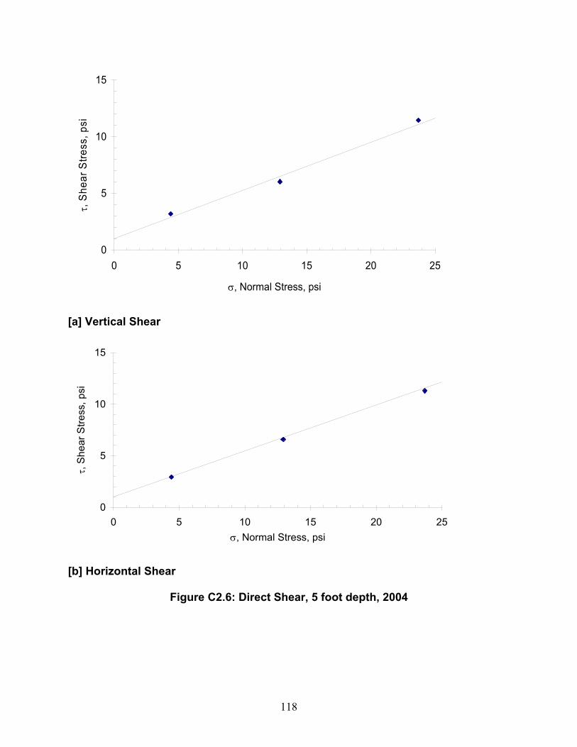
118
0
5
10
15
0 5 10 15 20 25
σ, Normal Stress, psi
τ, S
hear
Stre
ss, p
si
[a] Vertical Shear
0
5
10
15
0 5 10 15 20 25σ, Normal Stress, psi
τ, S
hear
Stre
ss, p
si
[b] Horizontal Shear
Figure C2.6: Direct Shear, 5 foot depth, 2004
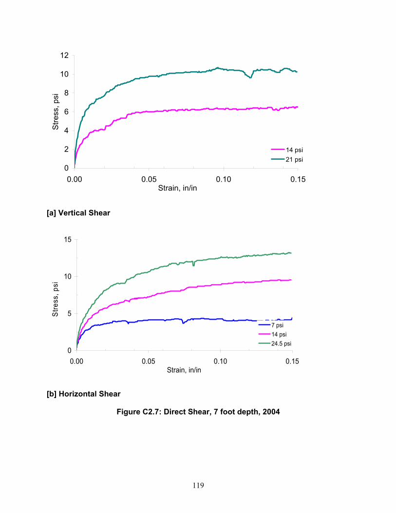
119
0
2
4
6
8
10
12
0.00 0.05 0.10 0.15Strain, in/in
Stre
ss, p
si
14 psi21 psi
[a] Vertical Shear
0
5
10
15
0.00 0.05 0.10 0.15Strain, in/in
Stre
ss, p
si
7 psi14 psi24.5 psi
[b] Horizontal Shear
Figure C2.7: Direct Shear, 7 foot depth, 2004
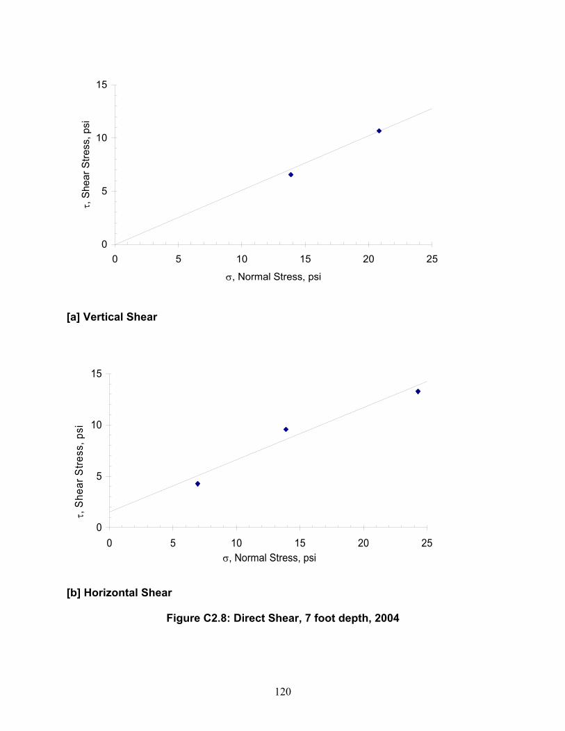
120
0
5
10
15
0 5 10 15 20 25
σ, Normal Stress, psi
τ, S
hear
Stre
ss, p
si
[a] Vertical Shear
0
5
10
15
0 5 10 15 20 25σ, Normal Stress, psi
τ, S
hear
Stre
ss, p
si
[b] Horizontal Shear
Figure C2.8: Direct Shear, 7 foot depth, 2004
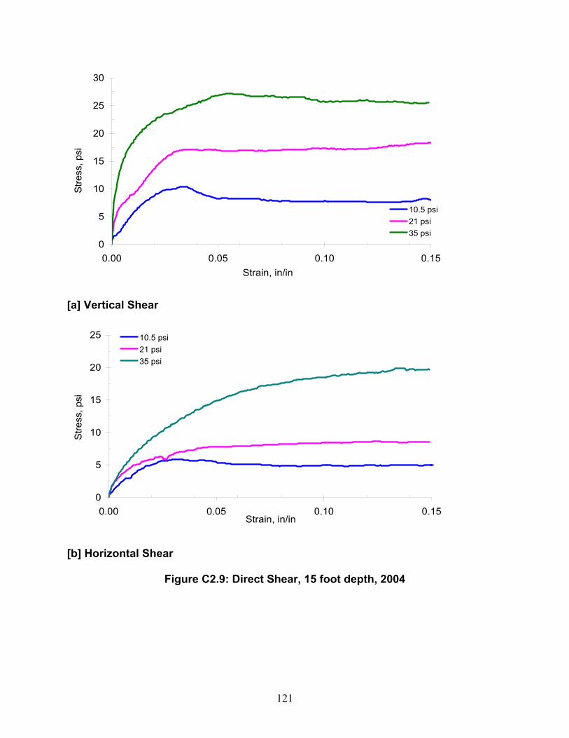
121
0
5
10
15
20
25
30
0.00 0.05 0.10 0.15Strain, in/in
Stre
ss, p
si
10.5 psi21 psi35 psi
[a] Vertical Shear
0
5
10
15
20
25
0.00 0.05 0.10 0.15Strain, in/in
Stre
ss, p
si
10.5 psi21 psi35 psi
[b] Horizontal Shear
Figure C2.9: Direct Shear, 15 foot depth, 2004
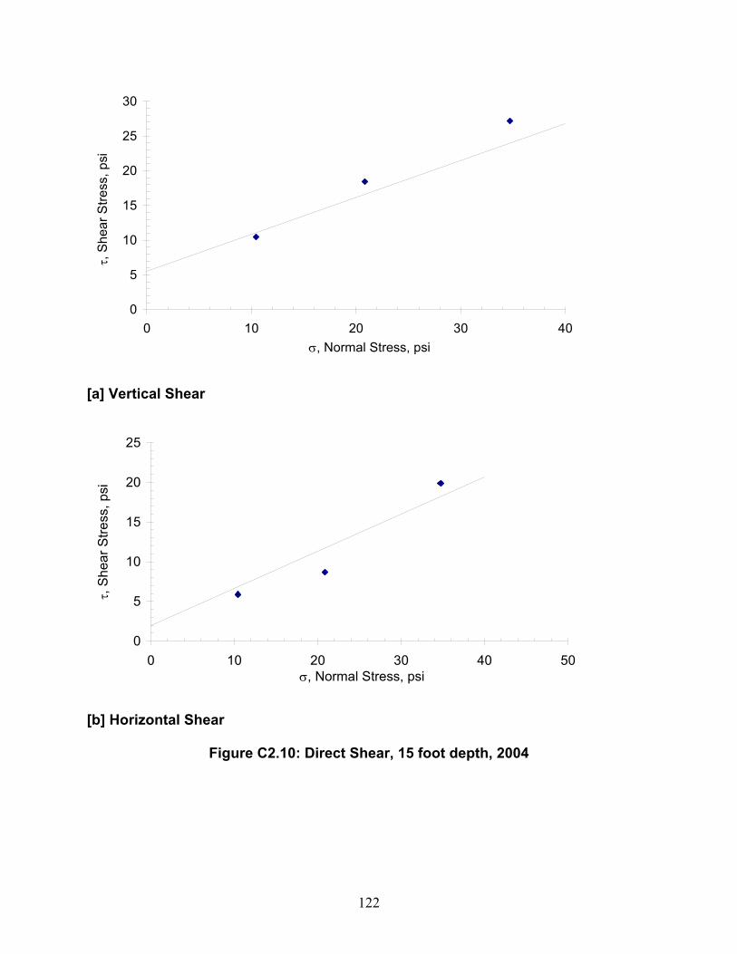
122
0
5
10
15
20
25
30
0 10 20 30 40σ, Normal Stress, psi
τ, S
hear
Stre
ss, p
si
[a] Vertical Shear
0
5
10
15
20
25
0 10 20 30 40 50σ, Normal Stress, psi
τ, S
hear
Stre
ss, p
si
[b] Horizontal Shear
Figure C2.10: Direct Shear, 15 foot depth, 2004
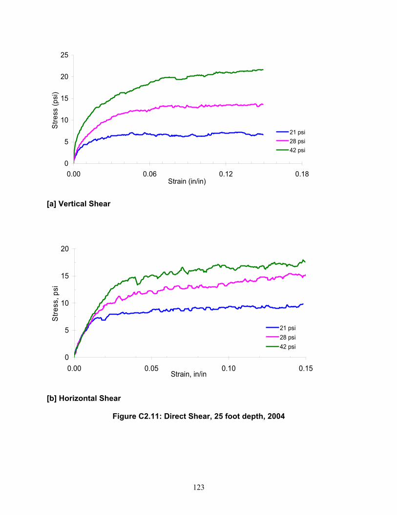
123
0
5
10
15
20
25
0.00 0.06 0.12 0.18Strain (in/in)
Stre
ss (p
si)
21 psi28 psi42 psi
[a] Vertical Shear
0
5
10
15
20
0.00 0.05 0.10 0.15Strain, in/in
Stre
ss, p
si
21 psi28 psi42 psi
[b] Horizontal Shear
Figure C2.11: Direct Shear, 25 foot depth, 2004
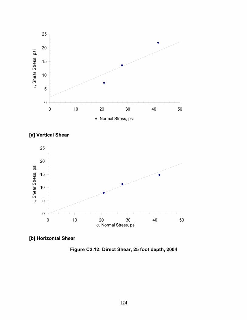
124
0
5
10
15
20
25
0 10 20 30 40 50
σ, Normal Stress, psi
τ, S
hear
Stre
ss, p
si
[a] Vertical Shear
0
5
10
15
20
25
0 10 20 30 40 50σ, Normal Stress, psi
τ, S
hear
Stre
ss, p
si
[b] Horizontal Shear
Figure C2.12: Direct Shear, 25 foot depth, 2004
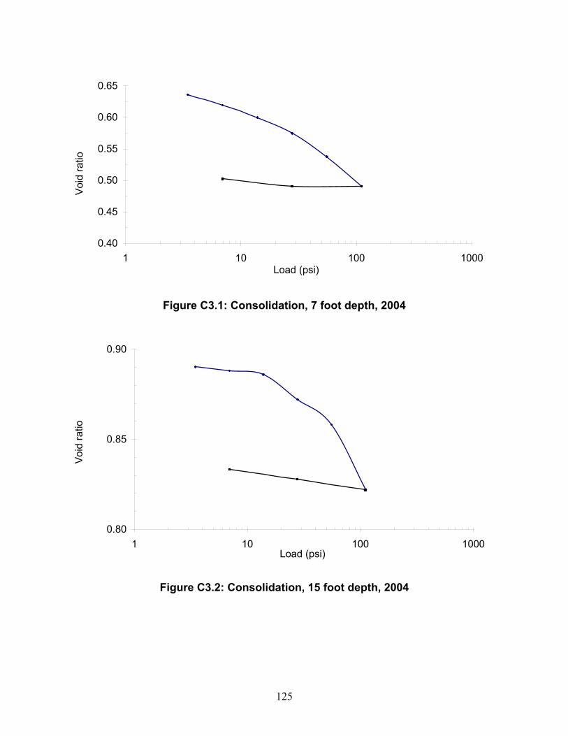
125
0.40
0.45
0.50
0.55
0.60
0.65
1 10 100 1000Load (psi)
Void
ratio
Figure C3.1: Consolidation, 7 foot depth, 2004
0.80
0.85
0.90
1 10 100 1000Load (psi)
Void
ratio
Figure C3.2: Consolidation, 15 foot depth, 2004
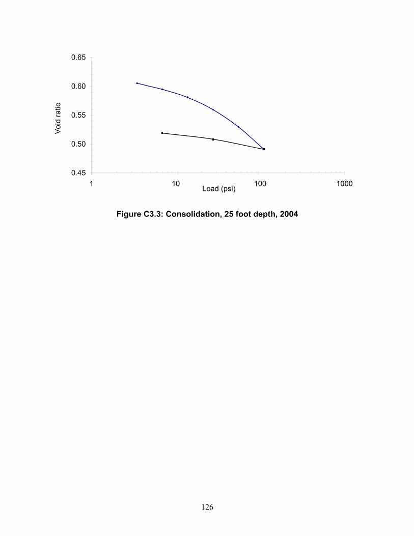
126
0.45
0.50
0.55
0.60
0.65
1 10 100 1000Load (psi)
Void
ratio
Figure C3.3: Consolidation, 25 foot depth, 2004
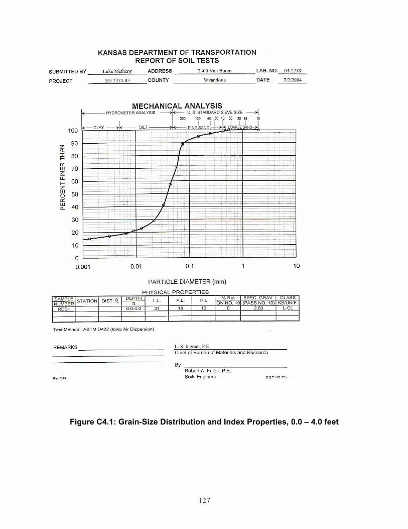
127
Figure C4.1: Grain-Size Distribution and Index Properties, 0.0 – 4.0 feet
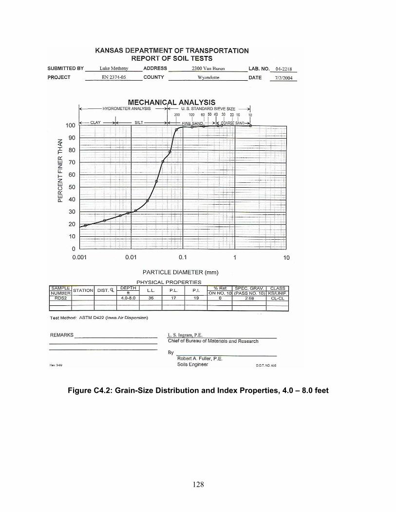
128
Figure C4.2: Grain-Size Distribution and Index Properties, 4.0 – 8.0 feet
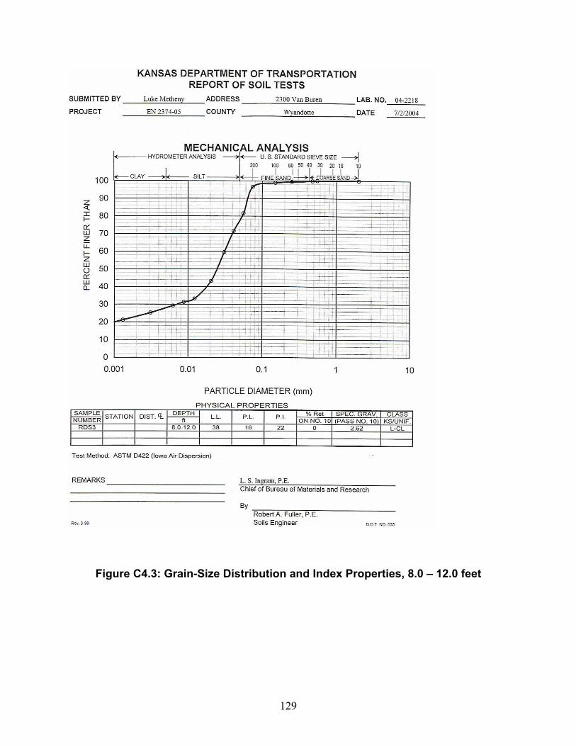
129
Figure C4.3: Grain-Size Distribution and Index Properties, 8.0 – 12.0 feet
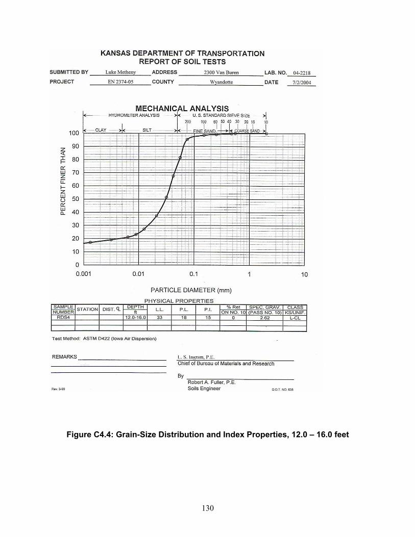
130
Figure C4.4: Grain-Size Distribution and Index Properties, 12.0 – 16.0 feet
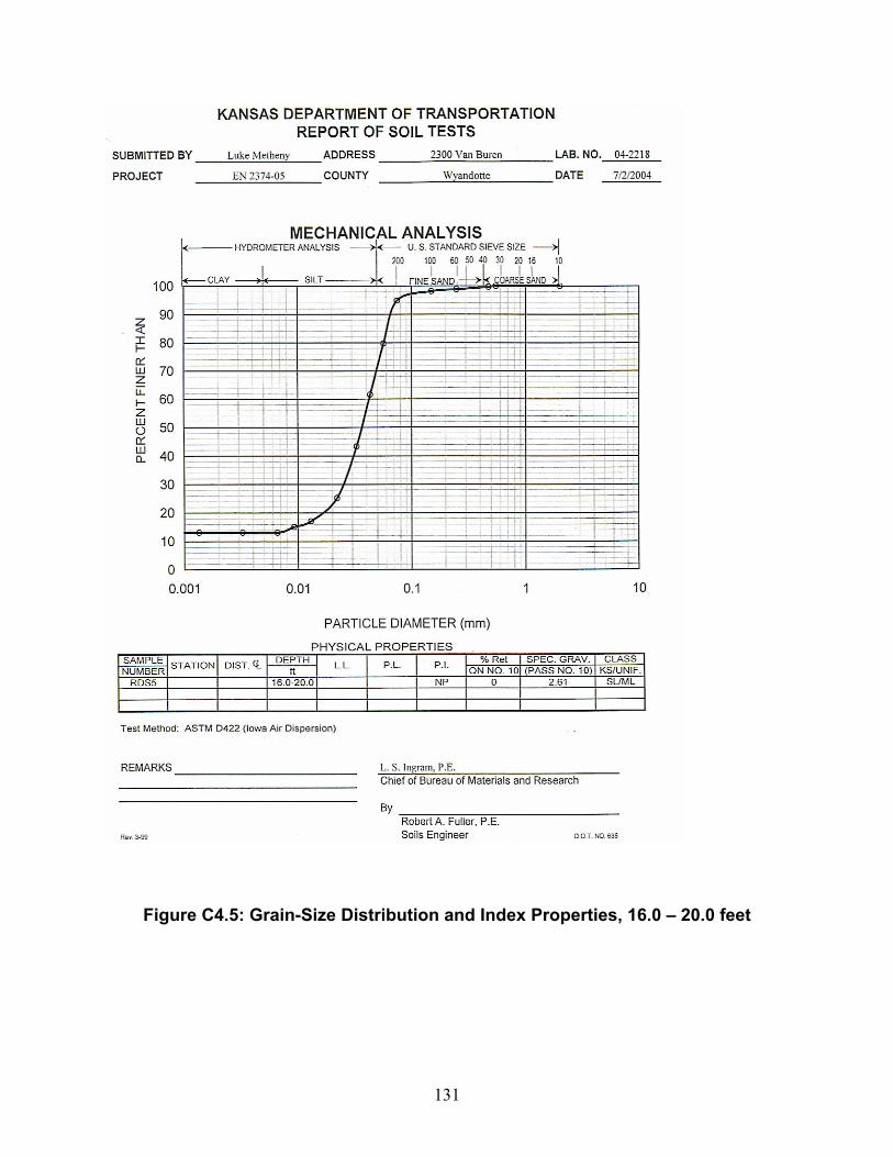
131
Figure C4.5: Grain-Size Distribution and Index Properties, 16.0 – 20.0 feet
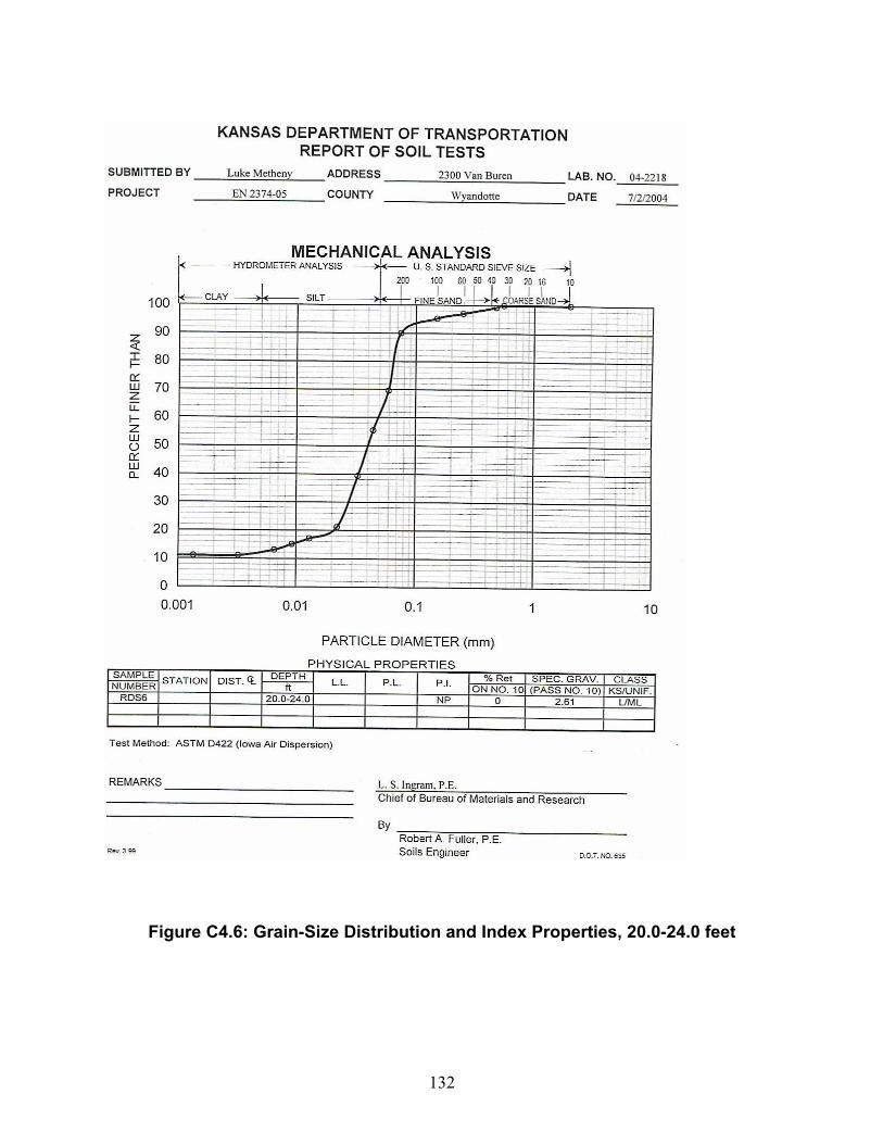
132
Figure C4.6: Grain-Size Distribution and Index Properties, 20.0-24.0 feet
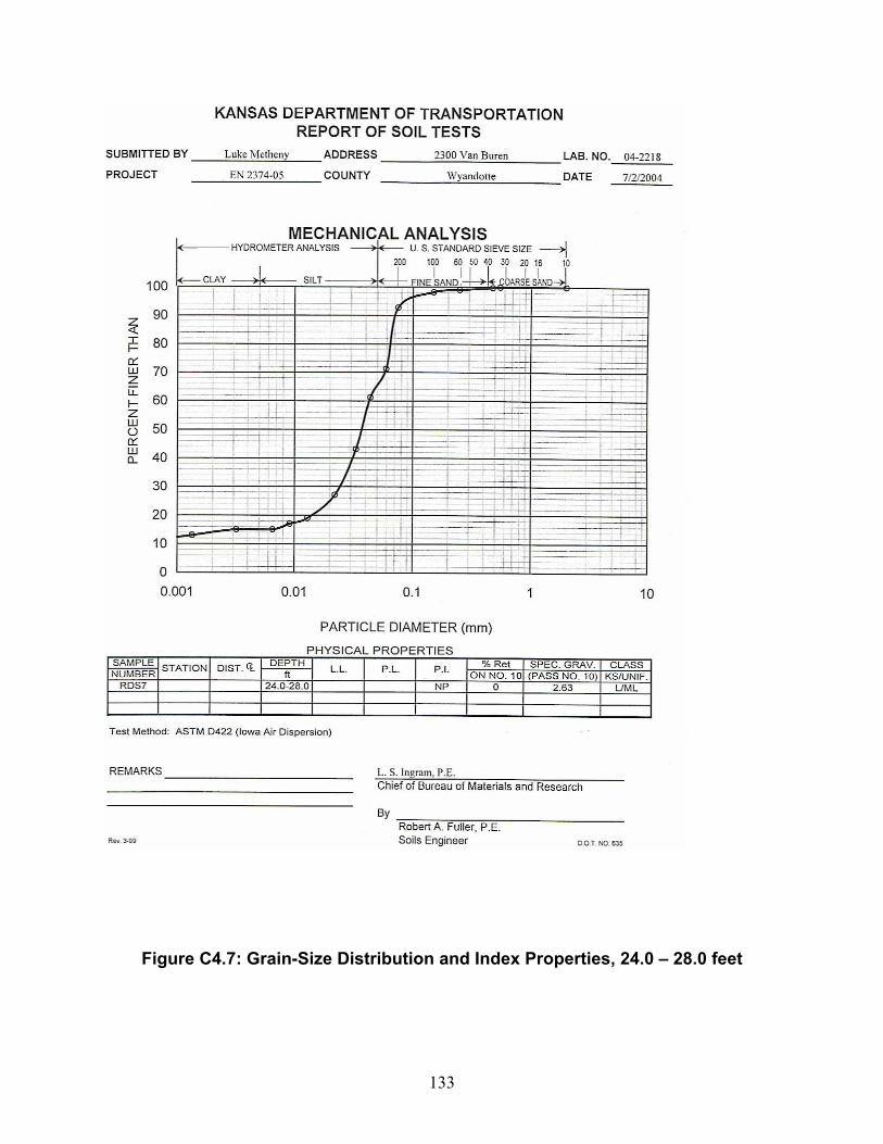
133
Figure C4.7: Grain-Size Distribution and Index Properties, 24.0 – 28.0 feet

134
Figure C4.8: Grain-Size Distribution and Index Properties, 28.0 – 32.0 feet
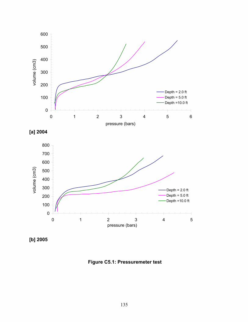
135
0
100
200
300
400
500
600
0 1 2 3 4 5 6pressure (bars)
volu
me
(cm
3)
Depth = 2.0 ftDepth = 5.0 ftDepth =10.0 ft
[a] 2004
0
100
200
300
400
500
600
700
800
0 1 2 3 4 5pressure (bars)
volu
me
(cm
3)
Depth = 2.0 ftDepth = 5.0 ftDepth =10.0 ft
[b] 2005
Figure C5.1: Pressuremeter test
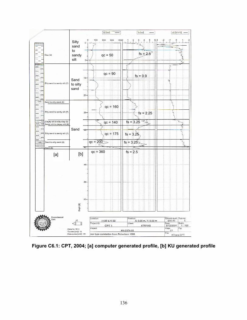
136
qc = 50
qc = 90
qc = 160
qc = 140
qc = 175
qc = 200
fs = 2.5
fs = 0.9
fs = 2.25
fs = 3.25
fs = 3.25
fs = 3.25
qc = 360 fs = 2.5
Silty sand to sandy silt
Sand to silty sand
Sand
[a] [b]
Figure C6.1: CPT, 2004; [a] computer generated profile, [b] KU generated profile
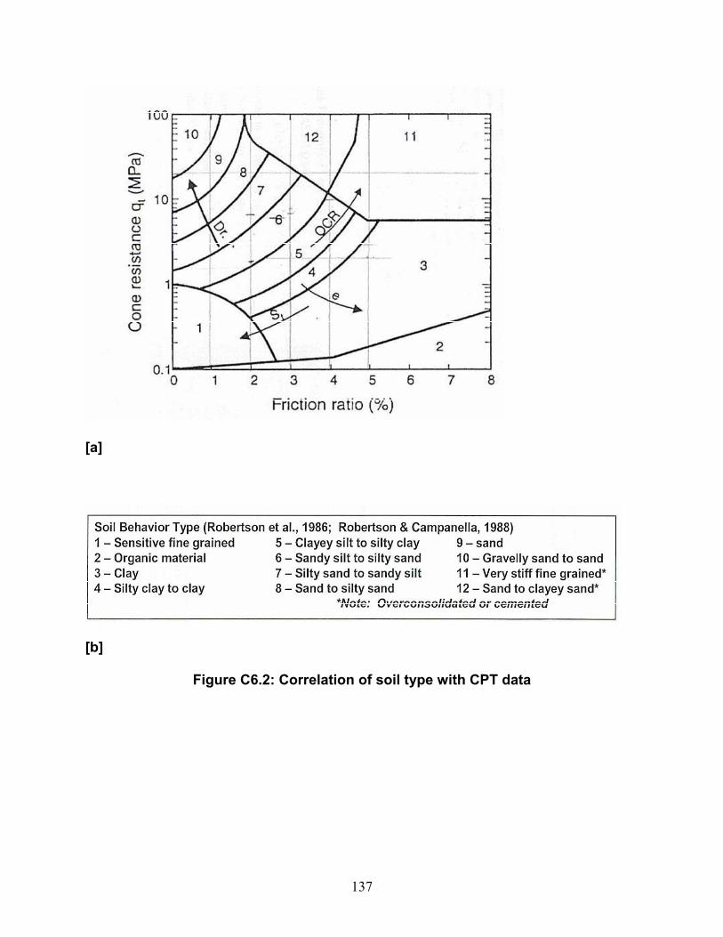
137
[a]
[b]
Figure C6.2: Correlation of soil type with CPT data
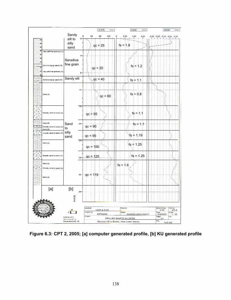
138
qc = 25
qc = 20
qc = 40
qc = 60
qc = 95
qc = 90
fs = 1.8
fs = 1.2
fs = 1.1
fs = 0.8
fs = 1.1
fs = 1.1
qc = 95
qc = 100
qc = 125
qc = 119
fs = 1.19
fs = 1.25
fs = 1.25
fs = 1.6
Sandy silt to silty sand
Sensitive fine grain
Sandy silt
Sand to silty sand
[a] [b]
Figure 6.3: CPT 2, 2005; [a] computer generated profile, [b] KU generated profile
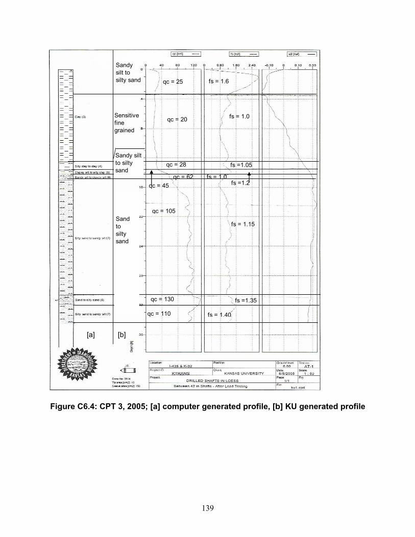
139
qc = 25
qc = 20
qc = 28
qc = 105
qc = 130
fs = 1.6
fs = 1.0
fs =1.05
fs = 1.15
fs =1.35
fs =1.2
qc = 110 fs = 1.40
qc = 62 fs = 1.0
[a] [b]
qc = 45
Sandy silt to silty sand
Sensitive fine grained
Sandy silt to silty sand
Sandto silty sand
Figure C6.4: CPT 3, 2005; [a] computer generated profile, [b] KU generated profile
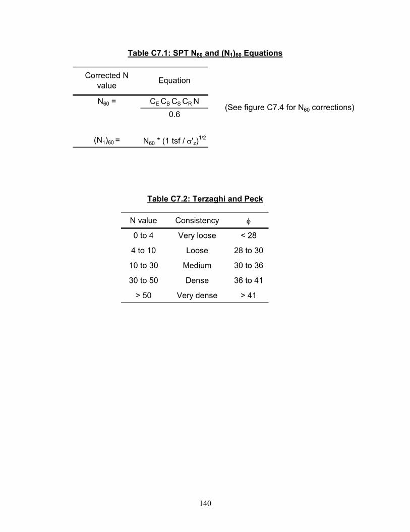
140
Table C7.1: SPT N60 and (N1)60 Equations
Corrected N value Equation
N60 = CE CB CS CR N0.6
(N1)60 = N60 * (1 tsf / σ'z)1/2
(See figure C7.4 for N60 corrections)
Table C7.2: Terzaghi and Peck
N value Consistency φ
0 to 4 Very loose < 28
4 to 10 Loose 28 to 30
10 to 30 Medium 30 to 36
30 to 50 Dense 36 to 41
> 50 Very dense > 41
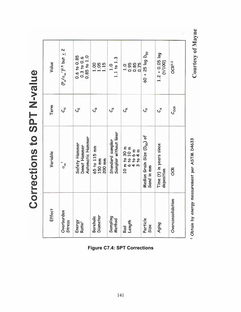
141
Figure C7.4: SPT Corrections
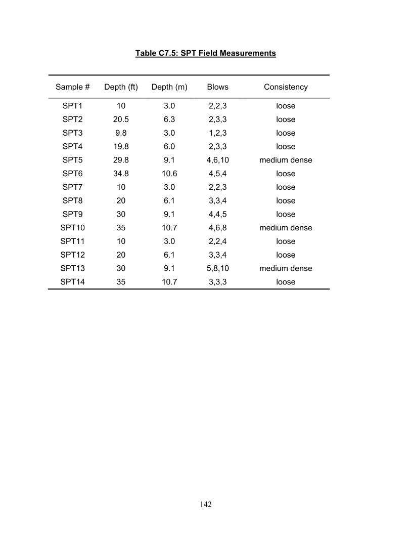
142
Table C7.5: SPT Field Measurements
Sample # Depth (ft) Depth (m) Blows Consistency
SPT1 10 3.0 2,2,3 loose
SPT2 20.5 6.3 2,3,3 loose
SPT3 9.8 3.0 1,2,3 loose
SPT4 19.8 6.0 2,3,3 loose
SPT5 29.8 9.1 4,6,10 medium dense
SPT6 34.8 10.6 4,5,4 loose
SPT7 10 3.0 2,2,3 loose
SPT8 20 6.1 3,3,4 loose
SPT9 30 9.1 4,4,5 loose
SPT10 35 10.7 4,6,8 medium dense
SPT11 10 3.0 2,2,4 loose
SPT12 20 6.1 3,3,4 loose
SPT13 30 9.1 5,8,10 medium dense
SPT14 35 10.7 3,3,3 loose
143
Appendix D
P-Y Model Derived from Lateral Load Testing
D.1 Introduction
A new method for generating P-Y curves for use in lateral analyses of drilled shafts in
loess soil is formulated, including degradation of the curves with load cycling. The P-Y
curves may be used for lateral analyses using any lateral analyses software package
that allows for input of user specified P-Y curves.
The strength parameter used in the model is correlated to the cone tip resistance
(qc) from CPT testing, and the rate at which the lateral resistance is gained with
displacement is presented as a hyperbolic relationship. Recommendations are
presented for the model parameters needed, as well as a discussion of their effect, as
were obtained from back-fitting of the LPILE analyses to the measured results.
The testing sequence and data reduction methods are presented, along with
comparisons of model analyses (LPILE used) to the measured results. A step-by-step
procedure is outlined for the use of the model presented to generate user specified P-Y
curves for lateral analyses.
D.2 Testing Sequence
Shafts were loaded in pairs to provide reaction for each other. Both shafts of a pair
were fully instrumented. There was one pair of 30-inch diameter static test shafts, one
pair of 42-inch diameter static test shafts, and one pair of 30-inch diameter cyclic test
shafts. Loads were maintained near constant at load increments without inclinometer
soundings, and the hydraulic pressure was locked off during load increments with
144
inclinometer soundings to better maintain the deflected pile shape with depth. A more
thorough description of the testing set-up and sequence is contained in Chapter 3.
A total of 13 and 15 load increments were used to load the 30-inch and 42 inch
diameters pairs of static test piles, respectively, while both sets of static test piles were
unloaded in four decrements. A total of six inclinometer soundings were performed for
each static test pile, four of which occurred at load increments. Load increments and
decrements for the static test shafts were sustained for a duration of approximately 5
minutes, with the exception of the load increments with inclinometer soundings where
the duration was approximately 20 minutes (this allowed for approximately 10 minutes
for inclinometer measurements for each of the two test shafts in the pair). Lateral loads
were applied to the 30-inch and 42-inch diameter static test shafts in approximately 10
kip and 15 kip increments, respectively.
There were a total of four load increments (noted as “A” through “D”) on the 30-
inch diameter cyclic test shafts, with ten load cycles (N=1 through 10) performed per
load increment. The lateral load for each load cycle were sustained for only a few
seconds with the exception of load cycles 1 and 10 which were sustained for
approximately 15 to 20 minutes to allow time for the inclinometer soundings to be
performed. For load cycles 2 through 9, the duration for each load cycle was
approximately 1 minute, 2 minutes, 3.5 minutes, and 6.5 minutes for load increments A
though D, respectively, as a greater time was required to reach the larger loads. The
load was reversed after each load cycle to return the top of pile to approximately the
same location.
145
D.3 Idealized Model Profile from CPT Testing
A back-fit model of the pile behavior using the variety of soil strength data obtained
(both insitu and laboratory) to the measured pile performance led to the conclusion that
the CPT testing provided the best correlation. Further, CPT testing is easily performed
in the loess soils being modeled, and has become readily available to practicing
geotechnical engineers and DOT’s. A brief description of CPT testing performed at the
site, and the idealization of the tip resistance (qc) with depth profile used subsequently
in the model is presented to follow. Complete descriptions of site characterization by
means of insitu testing, lab testing, soil classification, etc., is detailed in Chapter 4.
A total of three Cone Penetration Test (CPT) soundings were performed by
KDOT at the test site location, and the resulting subsurface profiles are contained in
Appendix C. A preliminary sounding was performed on 12 Aug 2004 in the general
vicinity of the test shafts (CPT-1). Two CPT soundings were performed subsequent to
the lateral load testing. A sounding performed on 8 June 2005 between the 42-inch
diameter static test shafts (Shafts 1 and 2) shortly after the completion the load test
performed on these shafts that same day. A sounding was performed on 9 June 2005
between the 30-inch diameter static test shafts (Shafts 3 and 4) two days after the
completion of the load test performed on these shafts on 7 June 2005. The CPT
sounding locations were approximately 5 to 6 feet away from their respective test
shafts, and given the nature of the soil condition and the albescence of a ground water
table at these elevations it is reasonable to assume that the CPT soundings were
unaffected by any pore water pressure effects that may have been induced by the load
testing.
146
An idealized profile of cone tip resistance (qc) with depth interpreted as an
average from the CPT soundings performed between the static test shafts (8-9 June
2005) is shown on Figure 1. This profile is considered representative of the subsurface
conditions for all the test shaft locations (test shafts 1 – 6). Note that it is most useful to
break the idealized soil profile into layers wherein the cone tip resistance (qc) is either
constant with depth or linearly varies with depth as these two conditions are easily
accommodated by most lateral pile analyses software.
The representative cone tip resistance (qc) is reduced by 50% at the soil surface,
and allowed to return to the full value at a depth equal to two pile diameters, as is
illustrated in Figure D1. This is done to account for the passive wedge failure
mechanism exhibited at the ground surface which reduces the resistance per pile length
nearer the ground surface until at some depth (assumed at two diameters) the
resistance is considered to be a flow around bearing failure mechanism.
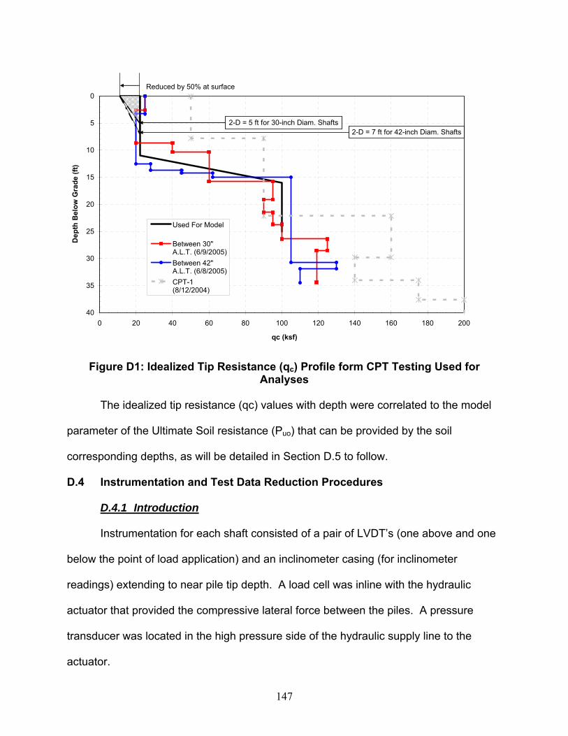
147
0
5
10
15
20
25
30
35
400 20 40 60 80 100 120 140 160 180 200
qc (ksf)
Dep
th B
elow
Gra
de (f
t)
Used For Model
Between 30"A.L.T. (6/9/2005)Between 42"A.L.T. (6/8/2005)CPT-1(8/12/2004)
Reduced by 50% at surface
2-D = 5 ft for 30-inch Diam. Shafts2-D = 7 ft for 42-inch Diam. Shafts
Figure D1: Idealized Tip Resistance (qc) Profile form CPT Testing Used for Analyses
The idealized tip resistance (qc) values with depth were correlated to the model
parameter of the Ultimate Soil resistance (Puo) that can be provided by the soil
corresponding depths, as will be detailed in Section D.5 to follow.
D.4 Instrumentation and Test Data Reduction Procedures
D.4.1 Introduction
Instrumentation for each shaft consisted of a pair of LVDT’s (one above and one
below the point of load application) and an inclinometer casing (for inclinometer
readings) extending to near pile tip depth. A load cell was inline with the hydraulic
actuator that provided the compressive lateral force between the piles. A pressure
transducer was located in the high pressure side of the hydraulic supply line to the
actuator.
148
For each pile, the test shaft data of the two LVDT displacements, the load cell,
and the pressure transducer were continuously monitored using a Megadac® data
acquisition system with the sampling rate set at 1 sample every 3 seconds for each
channel. At the prescribed load intervals, an inclinometer sounding was performed for
each test shaft by KDOT, with data points taken at 2 foot depth intervals.
D.4.2 Load Cell Readings and Hydraulic Pressure Transducer to Provide
Load
A load cell was inline with the hydraulic actuator that provided the compressive
lateral force between the piles. A pressure transducer was located in the high pressure
side of the hydraulic supply line to the actuator for an indirect back-up to the applied
load readings made directly by the load cell. Inspection of the data reveals that the load
cell provided reliable direct readings of the applied load.
D.4.3 LVDT Readings to Provide Boundary Condition at Top of Shaft
Each Test shaft was instrumented with two LVDT’s, one approximately 6 inches
above and one approximately 6 inches below the point of load application (see Chapter
3 for full details and as-builts of the test shafts). The LVDT’s provided a direct
measurement of the top of shaft movement for each test shaft.
For the Static test shafts, each LVDT measurement was averaged for the
duration of each load increment, which was an approximate 20 minute hold time for load
increments with inclinometer soundings (10 minutes each for two shafts).
For Load Cycles 2 through 9 of the Cyclic test shafts (load cycles without
inclinometer soundings), each LVDT measurement was averaged for the duration of
each load increment (approximate hold times of only several seconds). For Load
149
Cycles 1 and 10 of the Cyclic test shafts (load cycles with inclinometer soundings), each
LVDT measurement was averaged near the onset of the applied load for a duration that
corresponded to that of the other load cycles (i.e., the first several seconds of the
approximately 20 minutes that it took to run the inclinometer soundings).
In addition to providing top of shaft deflections, the two LVDT data points near
the top of each pile were used to provide the pile displacement boundary condition
(absolute displacement) corresponding to the uppermost inclinometer data point
location. The displacement of the uppermost inclinometer data point was interpolated
from the two LVDT data points if it was above the lower LVDT, and extrapolated if below
the lower LVDT. This linear interpolation, or extrapolation, is valid due to the close
proximity of the first inclinometer data point to the lower LVDT (typically within a few
inches), and these data points lying approximately 3 ft above grade.
D.4.4 Inclinometer Readings to Provide Deflected Pile Shape
For each of the static test shafts, an inclinometer sounding was performed:
• prior to loading to provide a baseline profile to obtain the deflected
profiles;
• at four load increments that were chosen to span the range of pile head
displacements to the ultimate load (approximately 0.5, 1.0, 2.3, and 4.0
inches);
• at the midpoint of the load decrements; and
• at the end of testing after the load was completely released.
150
Note that for each of the cyclic test shafts, an inclinometer sounding was
performed:
• prior to loading to provide a baseline profile to obtain the deflected
profiles;
• at the first and last load cycles (N=1 and N=10) for each of the four load
increments (A through D). Note that the four load increments were
chosen such that the respective pile head displacements at the first load
cycle (N=1) would be at approximately the same as for the static test
shafts; and
• at the end of testing after the load was completely released.
See Appendix A for detailed descriptions of load increments and inclinometer
soundings.
The inclinometer soundings were fixed at the depth of the first inclinometer
sounding data point below the top of each respective shaft by the LVDT readings
providing this boundary condition. An off-set correction was then applied to the
inclinometer soundings based upon reasonable pile tip displacements. The off-set
correction method adjusts displacements proportional to depth (as is the common
practice for reduction of inclinometer data). The inclinometer readings provide the
deflected pile profile and depth to maximum moment for comparison to that obtained
with the LPILE computer simulations.
D.5 Formulation of P-Y Model Parameters
D.5.1 Introduction
The static model parameters were developed upon best fits of full scale load test
data from two 30-inch and two 42-inch diameter shafts installed within a loess soil
151
formation with averaged CPT tip resistance values ranging from 20 to 105 ksf. Caution
is warranted when extrapolating the static model to predict results for shaft diameters or
soil types and/or strengths outside these limits. Further, the cyclic degradation model
parameters are based on sets of ten load cycles (N = 1 to 10) obtained at four different
load increments during the cyclic testing of an additional two 30-inch diameter shafts.
Caution is thus also warranted when extrapolating the cyclic model to predict results
beyond 10 load cycles (N>10), especially as the magnitude of the load increases.
Recommended procedures and correlation constants are provided to produce a
P-Y curve, shown generically in Figure D2, for any given soil layer. The Ultimate Soil
Resistance (Puo) that can be provided by the soil is simply correlated to the cone tip
resistance (qc) at any given elevation. Note that to account for the passive wedge
failure mechanism exhibited at the ground surface, the cone tip resistance (qc) is
reduced by 50% at the soil surface and allowed to return to the full value at a depth
equal to two pile diameters. The Initial modulus (Ei) of the P-Y curve is then determined
from the Ultimate Soil resistance (Puo) expressed on a per unit length of pile basis (Pu),
and a suggested reference displacement (Yi). A hyperbolic relationship provides the
Secant modulus (Es) of the P-Y curve at any given pile displacement (Y). The soil
resistance is then expressed on a per unit pile length basis (P) for any given pile
displacement (Y) as determined by the Secant modulus (Es) at that displacement.
Provisions for the degradation of the P-Y curve based upon the load cycle number (N)
for cyclic loading are incorporated into the relationship for Ultimate Soil resistance
expressed on a per unit length of pile basis (Pu).

152
Y (in)
P (lb
s/in
)Pu
Yi
Ei
Es
Y
P
Figure D2: Generic P-Y curve for Lateral Analyses
The model presented will generate a P-Y curve that is smooth and continuous. It
is believed that this better captures the true behavior of pile-to-soil response. The P-Y
curve may easily be generated with a spreadsheet using the functional relationships
presented that are expressed without the need for piece-wise continuity. Additionally,
this will also help to avoid convergence problems sometimes encountered with lateral
analyses software packages, as the iteration solutions often “bounce” around regions of
second order discontinuity (the “point” on bilinear curves, for example).
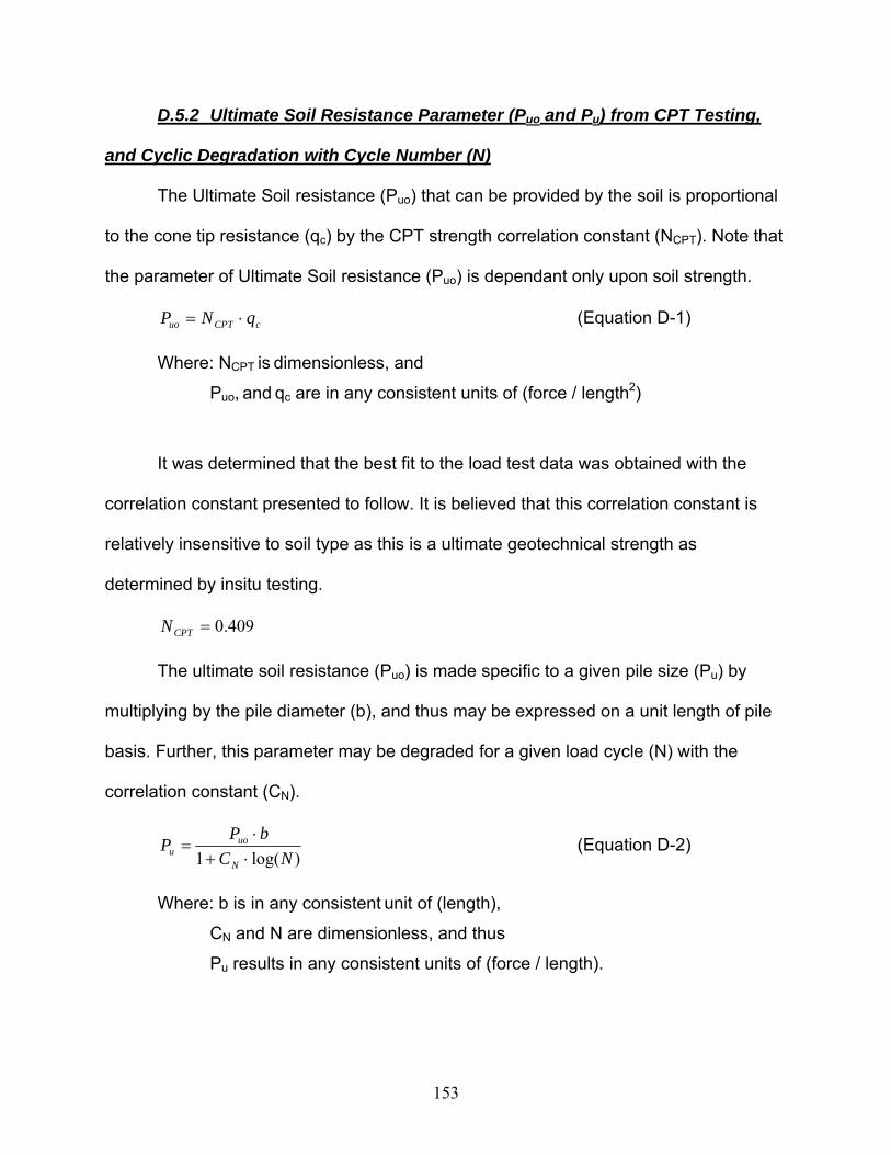
153
D.5.2 Ultimate Soil Resistance Parameter (Puo and Pu) from CPT Testing,
and Cyclic Degradation with Cycle Number (N)
The Ultimate Soil resistance (Puo) that can be provided by the soil is proportional
to the cone tip resistance (qc) by the CPT strength correlation constant (NCPT). Note that
the parameter of Ultimate Soil resistance (Puo) is dependant only upon soil strength.
cCPTuo qNP ⋅= (Equation D-1)
Where: NCPT is dimensionless, and
Puo, and qc are in any consistent units of (force / length2)
It was determined that the best fit to the load test data was obtained with the
correlation constant presented to follow. It is believed that this correlation constant is
relatively insensitive to soil type as this is a ultimate geotechnical strength as
determined by insitu testing.
409.0=CPTN
The ultimate soil resistance (Puo) is made specific to a given pile size (Pu) by
multiplying by the pile diameter (b), and thus may be expressed on a unit length of pile
basis. Further, this parameter may be degraded for a given load cycle (N) with the
correlation constant (CN).
)log(1 NCbP
PN
uou ⋅+
⋅= (Equation D-2)
Where: b is in any consistent unit of (length),
CN and N are dimensionless, and thus
Pu results in any consistent units of (force / length).
154
It was determined that the best fit of cyclic degradation to the two 30-inch
diameter shaft cyclic load test data was obtained with the following constant:
24.0=NC
The cyclic degradation term (denominator) reduces to 1 for N=1 (initial cycle, or
static load). The value of CN has a direct effect on the amount of cyclic degradation to
the P-Y curve (i.e., a greater value of CN will allow greater degradation of the P-Y curve,
resulting in a smaller Pu). Note that the degradation of the ultimate soil resistance per
unit length of shaft (Pu) parameter will also have the desired degradation effect built into
the computation of the P-Y modulus values (Ei and Es).
D.5.3 Reference Displacement Parameter (Yi)
A parameter is needed to define the rate at which the strength develops towards
its ultimate value (Puo). The reference displacement (Yi) is defined as the displacement
at which the tangent to the P-Y curve at zero displacement (Ei) intersects the Ultimate
Soil resistance asymptote (Pu), as was illustrated in Figure D2. For lateral displacement
of the pile-to-soil interface, this reference displacement (Yi) may be considered as
analogous to axial quake of a perfectly elastic-plastic bi-linear curve. It was determined
that the best fit to the load test data was obtained with the following reference
displacement (Yi).
Yi = 0.117 inches
Where: Yi is expressed in any consistent unit of (length).
Note that the suggested value for the reference displacement (Yi) provided the
best fit to the piles tested at one test site in a particular loess formation (see Chapter 5
for a full description of soil types). Unlike the ultimate geotechnical resistance (Puo), it is

155
believed that the rate at which the strength develops, represented by the reference
displacement (Yi), may be sensitive to soil type. Careful re-evaluation of the reference
displacement (Yi) parameter may be warranted when performing lateral analyses for
piles within different soil conditions, as this parameter may have substantial effect on
the resulting pile deflections and stresses. The effect of the reference displacement (Yi)
is direct to pile performance (i.e., a greater value of Yi will allow for greater pile head
displacements at a given lateral load).
D.5.4 Initial Modulus Parameter (Ei) and Hyperbolic Model of Secant
Modulus (Es)
By definition, the initial modulus (Ei) is a simple expression of the ultimate soil
resistance expressed on a per unit length of pile basis (Pu), and the reference
displacement (Yi).
i
ui Y
PE = (Equation D-3)
Where: Pu is in any consistent units of (force / length).
Yi is in any consistent units of (length), and thus
Es results in any consistent units of (force / length2).
The secant modulus (Es) may be determined for any given displacement (Y) by
the following hyperbolic relationship involving the initial modulus expressed on a per unit
length of pile basis (Ei) and a hyperbolic term (Y’h) which is in turn a function of the
given displacement (Y), the reference displacement (Yi), and a dimensionless
correlation constant (a).
h
is Y
EE
'1+= and (Equation D-4)
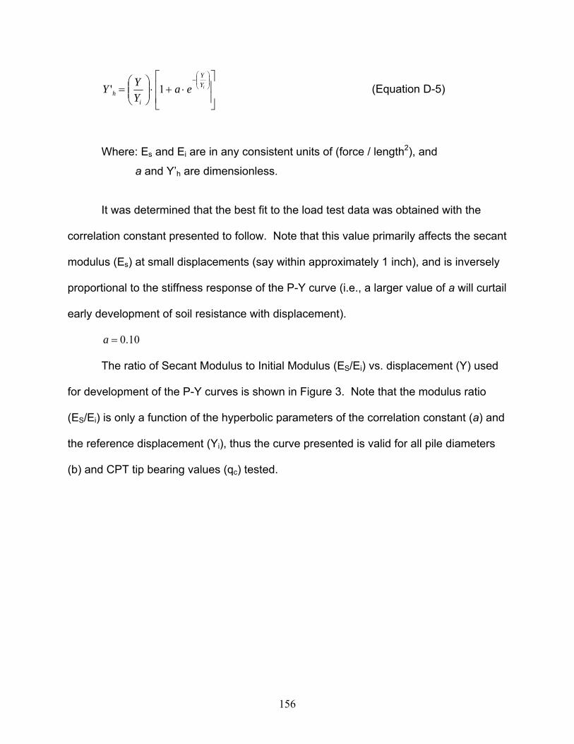
156
⎥⎥
⎦
⎤
⎢⎢
⎣
⎡⋅+⋅⎟⎟
⎠
⎞⎜⎜⎝
⎛=
⎟⎟⎠
⎞⎜⎜⎝
⎛−
iYY
ih ea
YYY 1' (Equation D-5)
Where: Es and Ei are in any consistent units of (force / length2), and
a and Y’h are dimensionless.
It was determined that the best fit to the load test data was obtained with the
correlation constant presented to follow. Note that this value primarily affects the secant
modulus (Es) at small displacements (say within approximately 1 inch), and is inversely
proportional to the stiffness response of the P-Y curve (i.e., a larger value of a will curtail
early development of soil resistance with displacement).
10.0=a
The ratio of Secant Modulus to Initial Modulus (ES/Ei) vs. displacement (Y) used
for development of the P-Y curves is shown in Figure 3. Note that the modulus ratio
(ES/Ei) is only a function of the hyperbolic parameters of the correlation constant (a) and
the reference displacement (Yi), thus the curve presented is valid for all pile diameters
(b) and CPT tip bearing values (qc) tested.
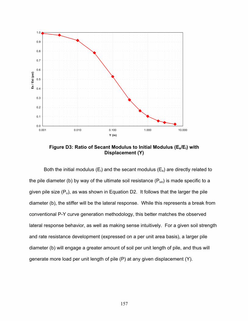
157
0.0
0.1
0.2
0.3
0.4
0.5
0.6
0.7
0.8
0.9
1.0
0.001 0.010 0.100 1.000 10.000
Y (in)
Es /
Esi (
psi)
Figure D3: Ratio of Secant Modulus to Initial Modulus (Es/Ei) with Displacement (Y)
Both the initial modulus (Ei) and the secant modulus (Es) are directly related to
the pile diameter (b) by way of the ultimate soil resistance (Puo) is made specific to a
given pile size (Pu), as was shown in Equation D2. It follows that the larger the pile
diameter (b), the stiffer will be the lateral response. While this represents a break from
conventional P-Y curve generation methodology, this better matches the observed
lateral response behavior, as well as making sense intuitively. For a given soil strength
and rate resistance development (expressed on a per unit area basis), a larger pile
diameter (b) will engage a greater amount of soil per unit length of pile, and thus will
generate more load per unit length of pile (P) at any given displacement (Y).
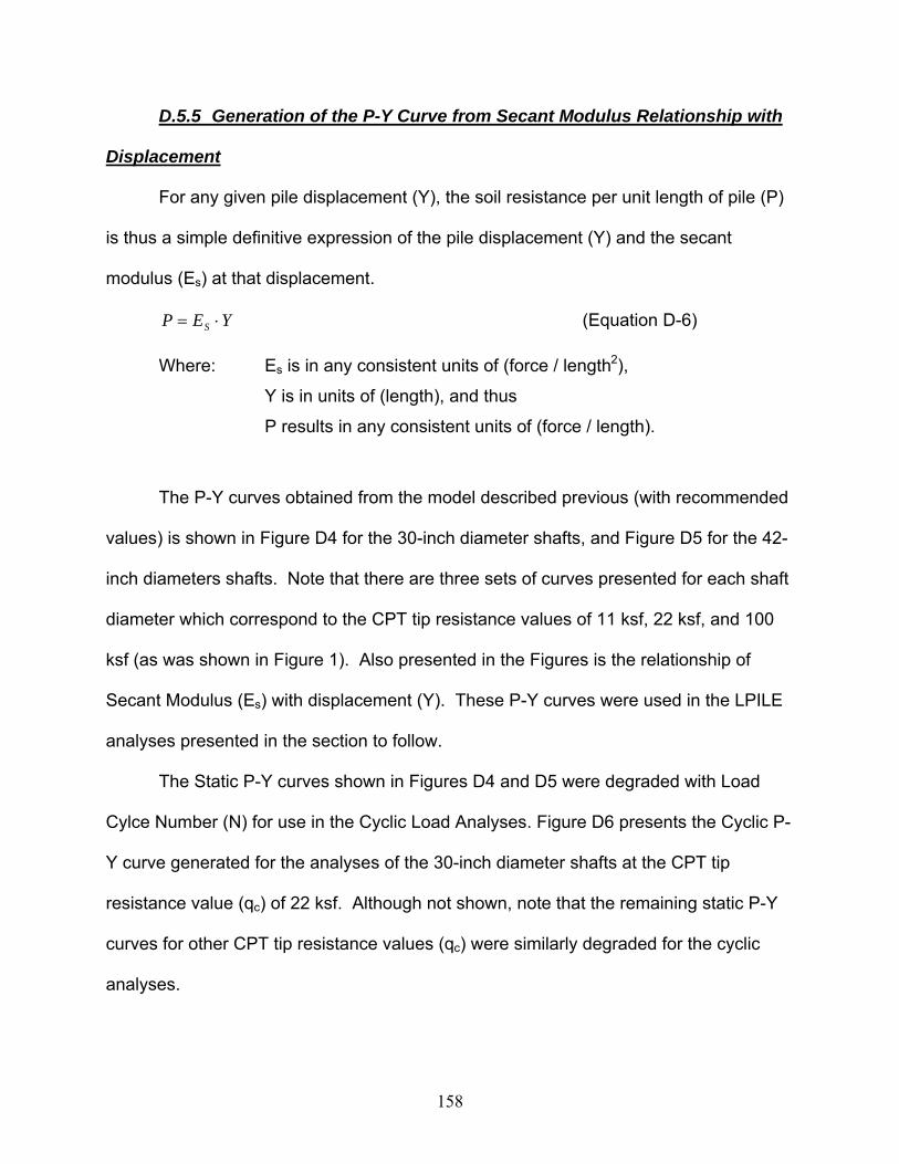
158
D.5.5 Generation of the P-Y Curve from Secant Modulus Relationship with
Displacement
For any given pile displacement (Y), the soil resistance per unit length of pile (P)
is thus a simple definitive expression of the pile displacement (Y) and the secant
modulus (Es) at that displacement.
YEP S ⋅= (Equation D-6)
Where: Es is in any consistent units of (force / length2),
Y is in units of (length), and thus
P results in any consistent units of (force / length).
The P-Y curves obtained from the model described previous (with recommended
values) is shown in Figure D4 for the 30-inch diameter shafts, and Figure D5 for the 42-
inch diameters shafts. Note that there are three sets of curves presented for each shaft
diameter which correspond to the CPT tip resistance values of 11 ksf, 22 ksf, and 100
ksf (as was shown in Figure 1). Also presented in the Figures is the relationship of
Secant Modulus (Es) with displacement (Y). These P-Y curves were used in the LPILE
analyses presented in the section to follow.
The Static P-Y curves shown in Figures D4 and D5 were degraded with Load
Cylce Number (N) for use in the Cyclic Load Analyses. Figure D6 presents the Cyclic P-
Y curve generated for the analyses of the 30-inch diameter shafts at the CPT tip
resistance value (qc) of 22 ksf. Although not shown, note that the remaining static P-Y
curves for other CPT tip resistance values (qc) were similarly degraded for the cyclic
analyses.

159
0
1,000
2,000
3,000
4,000
5,000
6,000
7,000
8,000
9,000
0.0 0.5 1.0 1.5 2.0 2.5 3.0 3.5 4.0 4.5 5.0 5.5 6.0Y (in)
E (p
si)
0
5,000
10,000
15,000
20,000
25,000
30,000
35,000
40,000
45,0000.0 0.5 1.0 1.5 2.0 2.5 3.0 3.5 4.0 4.5 5.0 5.5 6.0
P (lb
s/in
)
P
Esfor: CPT qc = 100 ksf (694 psi)
for: CPT qc = 11 ksf (76 psi)
for: CPT qc = 22 ksf (153 psi)
Figure D4: P-Y Curves and Secant Modulus (Es) for the 30-inch Diameter Shafts
0
1,000
2,000
3,000
4,000
5,000
6,000
7,000
8,000
9,000
10,000
11,000
12,000
0.0 0.5 1.0 1.5 2.0 2.5 3.0 3.5 4.0 4.5 5.0 5.5 6.0Y (in)
E (p
si)
0
10,000
20,000
30,000
40,000
50,000
60,000
70,000
80,000
90,000
100,000
110,000
120,0000.0 0.5 1.0 1.5 2.0 2.5 3.0 3.5 4.0 4.5 5.0 5.5 6.0
P (lb
s/in
)
P
Es
for: CPT qc = 100 ksf (694 psi)
for: CPT qc = 22 ksf (153 psi)
for: CPT qc = 11 ksf (76 psi)
Figure D5: P-Y Curves and Secant Modulus (Es) for the 42-inch Diameter Shafts
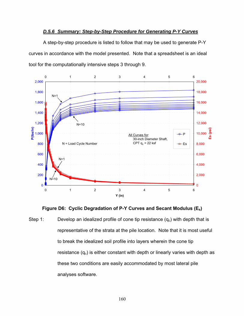
160
D.5.6 Summary: Step-by-Step Procedure for Generating P-Y Curves
A step-by-step procedure is listed to follow that may be used to generate P-Y
curves in accordance with the model presented. Note that a spreadsheet is an ideal
tool for the computationally intensive steps 3 through 9.
0
200
400
600
800
1,000
1,200
1,400
1,600
1,800
2,000
0 1 2 3 4 5 6
Y (in)
P(lb
s/in
)
0
2,000
4,000
6,000
8,000
10,000
12,000
14,000
16,000
18,000
20,0000 1 2 3 4 5 6
Es (p
si)
P
Es
All Curves for: 30-inch Diameter Shaft, CPT qc = 22 ksf
N=1
N=10
N=1
N=10
N = Load Cycle Number
Figure D6: Cyclic Degradation of P-Y Curves and Secant Modulus (Es) Step 1: Develop an idealized profile of cone tip resistance (qc) with depth that is
representative of the strata at the pile location. Note that it is most useful
to break the idealized soil profile into layers wherein the cone tip
resistance (qc) is either constant with depth or linearly varies with depth as
these two conditions are easily accommodated by most lateral pile
analyses software.
161
Step 2: For the purposes of lateral pile analyses, reduce the cone tip resistance
(qc) by 50% at the soil surface, and allowe the value to return to the full
measured value at a depth equal to two pile diameters. Linear
interpolation may be made between the surface and the depth of two pile
diameters.
Step 3: For each idealized soil layer, determine the ultimate soil resistance (Puo)
form the cone tip resistance (qc), in accordance with Equation D-1 for both
the top and the bottom of each layer.
Step 4: For the top and bottom of each idealized soil layer, multiply the ultimate
soil resistance (Puo) by the pile diameter to obtain the ultimate soil
resistance per unit length of shaft (Pu). For cyclic analyses, this parameter
(Pu) may be degraded for a given load cycle (N) with the correlation
constant (CN), in accordance with Equation D-2. Note that when running a
lateral pile analyses do NOT select the use of a P-Y multiplier, as the
cyclic degradation of the P-Y curve is already taken into account by use of
Equation D-2.
Step 5: For the top and bottom of each idealized soil layer, select a reference
displacement (Yi) that will be representative of the rate at which the
resistance will develop. Recommendations for values of reference
displacement (Yi) are presented in Section D.5.3.
Step 6: For the top and bottom of each idealized soil layer determine the initial
modulus (Ei) in accordance with Equation D-3.
162
Step 7: For the top and bottom of each idealized soil layer, select a number of
pile-to-soil displacements (Y) for which a representative P-Y curve is to be
generated. Make sure the largest of these values selected will be in
excess of the displacements anticipated for that layer, and note that soil
layers near the surface will experience much greater displacements than
those at greater depths. Concentrate the data points towards the smaller
displacements to better define the P-Y curve where the secant modulus
values (Es) are changing quickly (for example this study generated P-Y
curve data points at displacements of 0, 0.001, 0.003, 0.01, 0.03, 0.1, 0.3,
0.6, 1, 2, 3, and 6 inches).
Step 8: For the top and bottom of each idealized soil layer, determine the secant
modulus (Es) for each of the displacements selected in Step 7 in
accordance with Equations D-4 and D-5.
Step 9: For the top and bottom of each idealized soil layer, determine the soil
resistance per unit length of pile (P) for each of the displacements
selected in Step 7 in accordance with Equations D-6
Step 10: Run a lateral load analyses using “user specified P-Y” curves. The P-Y
curves are generated from the values of soil resistance per unit length of
pile (P) obtained in Step 9 that correspond to the displacement (Y)
obtained in Step 7.
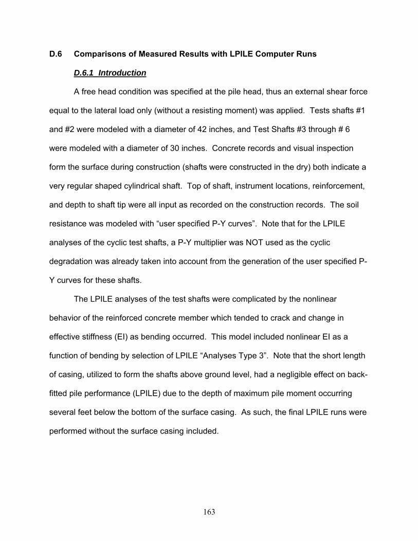
163
D.6 Comparisons of Measured Results with LPILE Computer Runs
D.6.1 Introduction
A free head condition was specified at the pile head, thus an external shear force
equal to the lateral load only (without a resisting moment) was applied. Tests shafts #1
and #2 were modeled with a diameter of 42 inches, and Test Shafts #3 through # 6
were modeled with a diameter of 30 inches. Concrete records and visual inspection
form the surface during construction (shafts were constructed in the dry) both indicate a
very regular shaped cylindrical shaft. Top of shaft, instrument locations, reinforcement,
and depth to shaft tip were all input as recorded on the construction records. The soil
resistance was modeled with “user specified P-Y curves”. Note that for the LPILE
analyses of the cyclic test shafts, a P-Y multiplier was NOT used as the cyclic
degradation was already taken into account from the generation of the user specified P-
Y curves for these shafts.
The LPILE analyses of the test shafts were complicated by the nonlinear
behavior of the reinforced concrete member which tended to crack and change in
effective stiffness (EI) as bending occurred. This model included nonlinear EI as a
function of bending by selection of LPILE “Analyses Type 3”. Note that the short length
of casing, utilized to form the shafts above ground level, had a negligible effect on back-
fitted pile performance (LPILE) due to the depth of maximum pile moment occurring
several feet below the bottom of the surface casing. As such, the final LPILE runs were
performed without the surface casing included.
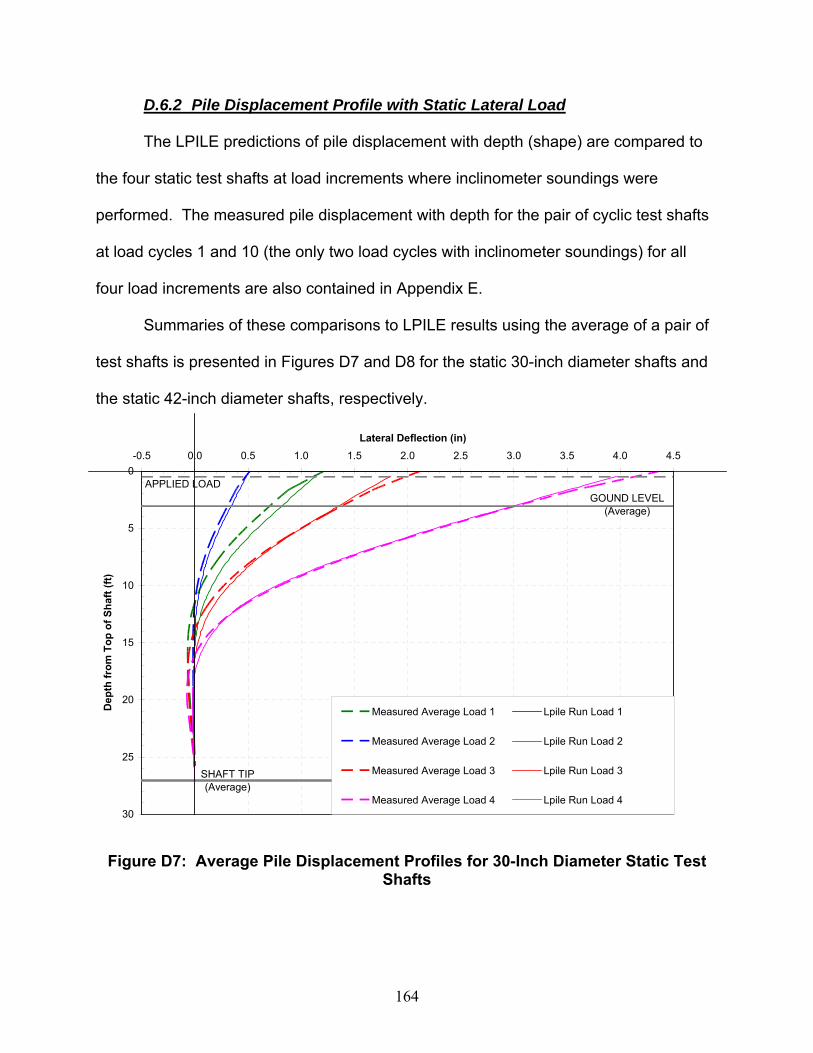
164
D.6.2 Pile Displacement Profile with Static Lateral Load
The LPILE predictions of pile displacement with depth (shape) are compared to
the four static test shafts at load increments where inclinometer soundings were
performed. The measured pile displacement with depth for the pair of cyclic test shafts
at load cycles 1 and 10 (the only two load cycles with inclinometer soundings) for all
four load increments are also contained in Appendix E.
Summaries of these comparisons to LPILE results using the average of a pair of
test shafts is presented in Figures D7 and D8 for the static 30-inch diameter shafts and
the static 42-inch diameter shafts, respectively.
GOUND LEVEL (Average)
SHAFT TIP (Average)
APPLIED LOAD0
5
10
15
20
25
30
-0.5 0.0 0.5 1.0 1.5 2.0 2.5 3.0 3.5 4.0 4.5
Lateral Deflection (in)
Dep
th fr
om T
op o
f Sha
ft (ft
)
Measured Average Load 1 Lpile Run Load 1
Measured Average Load 2 Lpile Run Load 2
Measured Average Load 3 Lpile Run Load 3
Measured Average Load 4 Lpile Run Load 4
Figure D7: Average Pile Displacement Profiles for 30-Inch Diameter Static Test Shafts
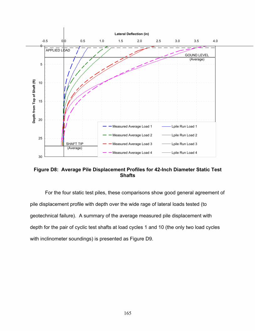
165
GOUND LEVEL (Average)
SHAFT TIP(Average)
APPLIED LOAD0
5
10
15
20
25
30
-0.5 0.0 0.5 1.0 1.5 2.0 2.5 3.0 3.5 4.0
Lateral Deflection (in)D
epth
from
Top
of S
haft
(ft)
Measured Average Load 1 Lpile Run Load 1
Measured Average Load 2 Lpile Run Load 2
Measured Average Load 3 Lpile Run Load 3
Measured Average Load 4 Lpile Run Load 4
Figure D8: Average Pile Displacement Profiles for 42-Inch Diameter Static Test Shafts
For the four static test piles, these comparisons show good general agreement of
pile displacement profile with depth over the wide rage of lateral loads tested (to
geotechnical failure). A summary of the average measured pile displacement with
depth for the pair of cyclic test shafts at load cycles 1 and 10 (the only two load cycles
with inclinometer soundings) is presented as Figure D9.
166
GOUND LEVEL (Average)
SHAFT TIP(Average)
APPLIED LOAD0
5
10
15
20
25
30
-0.5 0.0 0.5 1.0 1.5 2.0 2.5 3.0 3.5 4.0 4.5 5.0 5.5 6.0 6.5 7.0 7.5Lateral Deflection (in)
Dep
th fr
om T
op o
f Sha
ft (ft
)
Inclinometer Sounding No. 1 (Load No. A-1 = 50 kips)
Inclinometer Sounding No. 2 (Load No. A-10 = 49 kips)
Inclinometer Sounding No. 3 (Load No. B-1 = 76 kips)
Inclinometer Sounding No. 4 (Load No. B-10 = 77 kips)
Inclinometer Sounding No. 5 (Load No. C-1 = 106 kips)
Inclinometer Sounding No. 6 (Load No. C-10 = 112 kips)
Inclinometer Sounding No. 7 (Load No. D-1 = 137 kips)
Inclinometer Sounding No. 8 (Load No. D-10 = 136 kips)
Profiles Shown are Average of Shaft # 5 (N.E. Location)Shaft # 6 (N.W. Location)
Figure D9: Average Pile Displacement Profiles for 30-Inch Diameter Cyclic Test Shafts
D.6.3 Depth to Maximum Moment in Pile with Static Lateral Load
The comparison of magnitude and depth to maximum moment within a pile is
used for structural design of the pile. Figure D10 presents comparisons of depth to
maximum moment in the static test piles, to that obtained from corresponding LPILE
runs for the load increments where inclinometer soundings were performed. The depth
of maximum curvature of the test piles is determined as the point of maximum curvature
(i.e. the maximum change in slope). Although the magnitude of maximum moment was
not directly measured, the good agreement of depth to maximum moment between the
measured data and the LPILE runs obtained indicated a good agreement in magnitude
as well.
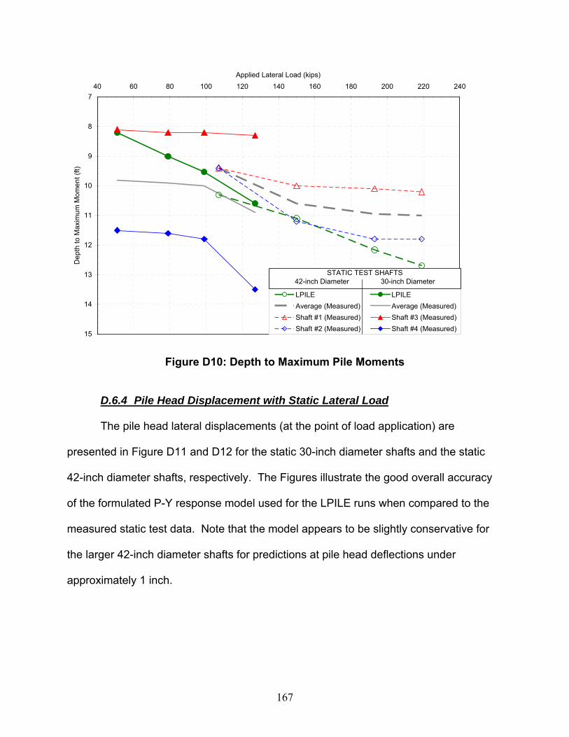
167
7
8
9
10
11
12
13
14
15
40 60 80 100 120 140 160 180 200 220 240Applied Lateral Load (kips)
Dep
th to
Max
imum
Mom
ent (
ft)
LPILE LPILEAverage (Measured) Average (Measured)Shaft #1 (Measured) Shaft #3 (Measured)Shaft #2 (Measured) Shaft #4 (Measured)
STATIC TEST SHAFTS42-inch Diameter 30-inch Diameter
Figure D10: Depth to Maximum Pile Moments
D.6.4 Pile Head Displacement with Static Lateral Load
The pile head lateral displacements (at the point of load application) are
presented in Figure D11 and D12 for the static 30-inch diameter shafts and the static
42-inch diameter shafts, respectively. The Figures illustrate the good overall accuracy
of the formulated P-Y response model used for the LPILE runs when compared to the
measured static test data. Note that the model appears to be slightly conservative for
the larger 42-inch diameter shafts for predictions at pile head deflections under
approximately 1 inch.
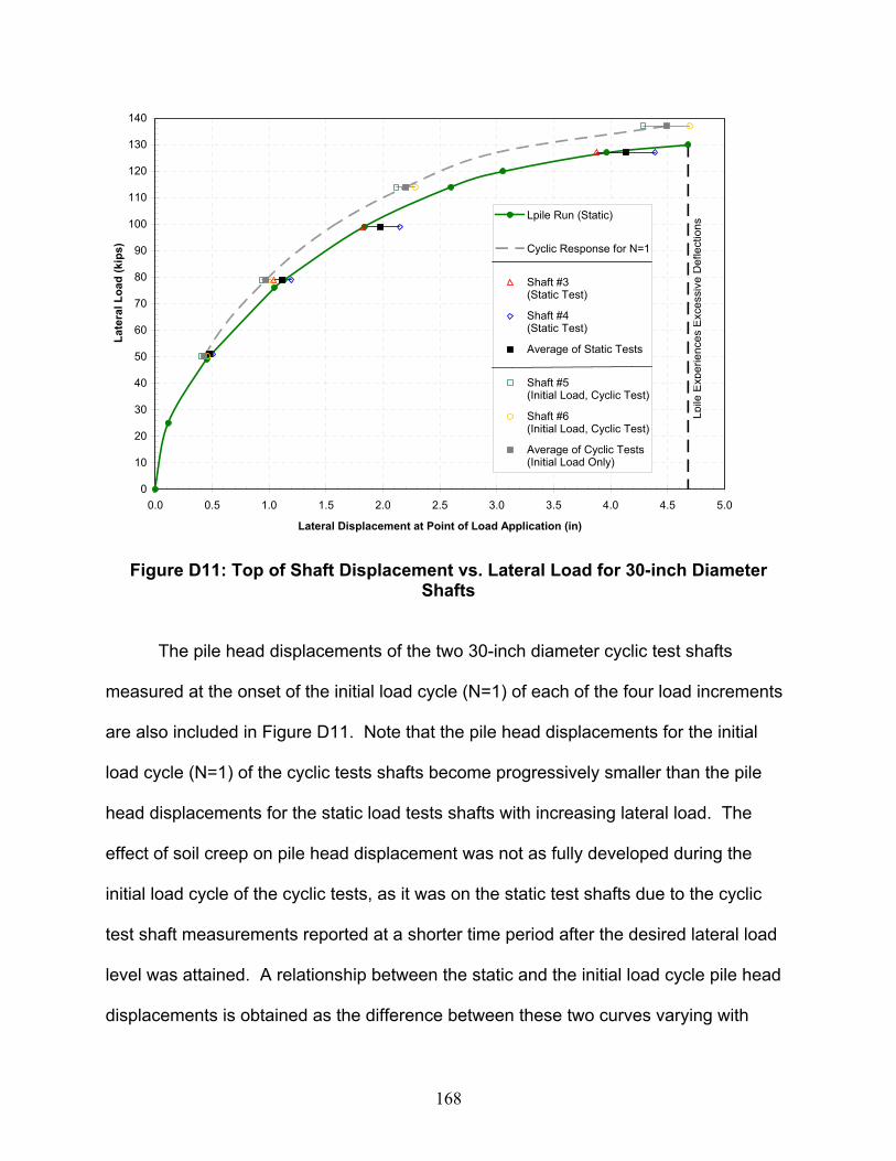
168
0
10
20
30
40
50
60
70
80
90
100
110
120
130
140
0.0 0.5 1.0 1.5 2.0 2.5 3.0 3.5 4.0 4.5 5.0
Lateral Displacement at Point of Load Application (in)
Late
ral L
oad
(kip
s)
Lpile Run (Static)
Cyclic Response for N=1
Shaft #3 (Static Test)
Shaft #4 (Static Test)
Average of Static Tests
Shaft #5 (Initial Load, Cyclic Test)
Shaft #6 (Initial Load, Cyclic Test)
Average of Cyclic Tests (Initial Load Only)
Lpile
Exp
erie
nces
Exc
essi
ve D
efle
ctio
ns
Figure D11: Top of Shaft Displacement vs. Lateral Load for 30-inch Diameter Shafts
The pile head displacements of the two 30-inch diameter cyclic test shafts
measured at the onset of the initial load cycle (N=1) of each of the four load increments
are also included in Figure D11. Note that the pile head displacements for the initial
load cycle (N=1) of the cyclic tests shafts become progressively smaller than the pile
head displacements for the static load tests shafts with increasing lateral load. The
effect of soil creep on pile head displacement was not as fully developed during the
initial load cycle of the cyclic tests, as it was on the static test shafts due to the cyclic
test shaft measurements reported at a shorter time period after the desired lateral load
level was attained. A relationship between the static and the initial load cycle pile head
displacements is obtained as the difference between these two curves varying with
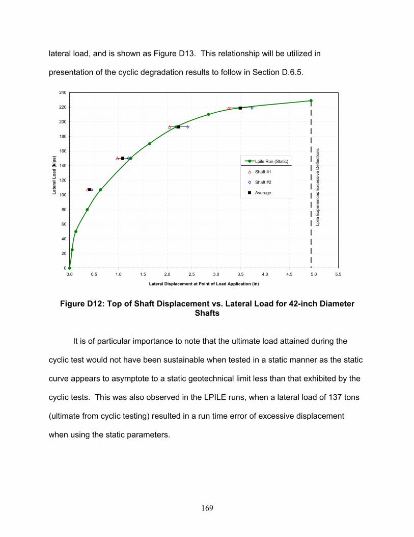
169
lateral load, and is shown as Figure D13. This relationship will be utilized in
presentation of the cyclic degradation results to follow in Section D.6.5.
0
20
40
60
80
100
120
140
160
180
200
220
240
0.0 0.5 1.0 1.5 2.0 2.5 3.0 3.5 4.0 4.5 5.0 5.5
Lateral Displacement at Point of Load Application (in)
Late
ral L
oad
(kip
s)
Lpile Run (Static)
Shaft #1
Shaft #2
Average
Lpile
Exp
erie
nces
Exc
essi
ve D
efle
ctio
ns
Figure D12: Top of Shaft Displacement vs. Lateral Load for 42-inch Diameter Shafts
It is of particular importance to note that the ultimate load attained during the
cyclic test would not have been sustainable when tested in a static manner as the static
curve appears to asymptote to a static geotechnical limit less than that exhibited by the
cyclic tests. This was also observed in the LPILE runs, when a lateral load of 137 tons
(ultimate from cyclic testing) resulted in a run time error of excessive displacement
when using the static parameters.
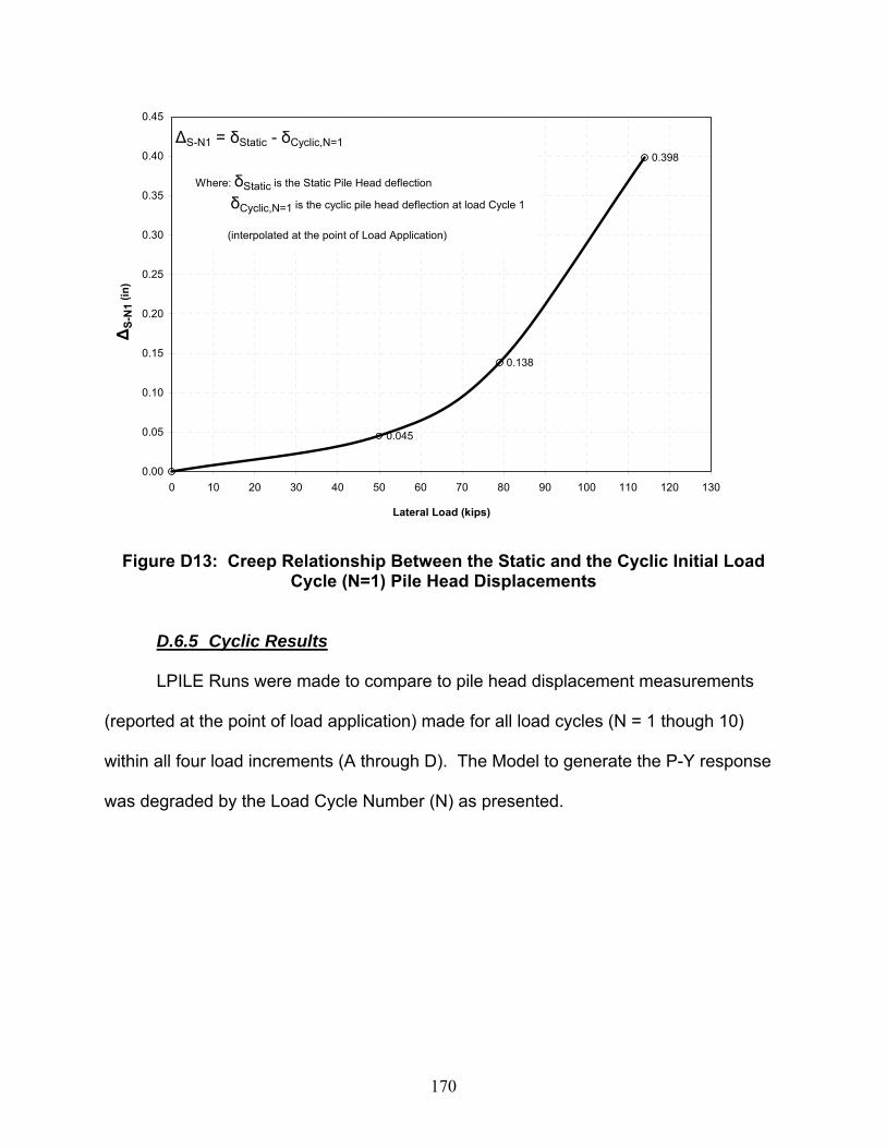
170
0.045
0.138
0.398
0.00
0.05
0.10
0.15
0.20
0.25
0.30
0.35
0.40
0.45
0 10 20 30 40 50 60 70 80 90 100 110 120 130
Lateral Load (kips)
ΔS-
N1
(in)
ΔS-N1 = δStatic - δCyclic,N=1
Where: δStatic is the Static Pile Head deflection
δCyclic,N=1 is the cyclic pile head deflection at load Cycle 1
(interpolated at the point of Load Application)
Figure D13: Creep Relationship Between the Static and the Cyclic Initial Load Cycle (N=1) Pile Head Displacements
D.6.5 Cyclic Results
LPILE Runs were made to compare to pile head displacement measurements
(reported at the point of load application) made for all load cycles (N = 1 though 10)
within all four load increments (A through D). The Model to generate the P-Y response
was degraded by the Load Cycle Number (N) as presented.
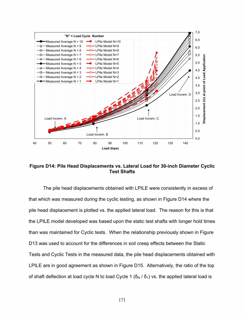
171
0.0
0.5
1.0
1.5
2.0
2.5
3.0
3.5
4.0
4.5
5.0
5.5
6.0
6.5
7.0
40 50 60 70 80 90 100 110 120 130 140Load (kips)
Dis
plac
emen
t (in
) at p
oint
of L
oad
App
licat
ion
Measured Average N = 10 LPile Model N=10Measured Average N = 9 LPile Model N=9Measured Average N = 8 LPile Model N=8Measured Average N = 7 LPile Model N=7Measured Average N = 6 LPile Model N=6Measured Average N = 5 LPile Model N=5Measured Average N = 4 LPile Model N=4Measured Average N = 3 LPile Model N=3Measured Average N = 2 LPile Model N=2Measured Average N = 1 LPile Model N=1
"N" = Load Cycle Number
Load Increm. A
Load Increm. B
Load Increm. C
Load Increm. D
Figure D14: Pile Head Displacements vs. Lateral Load for 30-inch Diameter Cyclic
Test Shafts
The pile head displacements obtained with LPILE were consistently in excess of
that which was measured during the cyclic testing, as shown in Figure D14 where the
pile head displacement is plotted vs. the applied lateral load. The reason for this is that
the LPILE model developed was based upon the static test shafts with longer hold times
than was maintained for Cyclic tests. When the relationship previously shown in Figure
D13 was used to account for the differences in soil creep effects between the Static
Tests and Cyclic Tests in the measured data, the pile head displacements obtained with
LPILE are in good agreement as shown in Figure D15. Alternatively, the ratio of the top
of shaft deflection at load cycle N to load Cycle 1 (δN / δ1) vs. the applied lateral load is
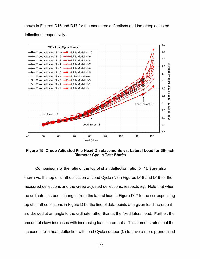
172
shown in Figures D16 and D17 for the measured deflections and the creep adjusted
deflections, respectively.
0.0
0.5
1.0
1.5
2.0
2.5
3.0
3.5
4.0
4.5
5.0
5.5
6.0
40 50 60 70 80 90 100 110 120Load (kips)
Dis
plac
emen
t (in
) at p
oint
of L
oad
App
licat
ion
Creep Adjusted N = 10 LPile Model N=10Creep Adjusted N = 9 LPile Model N=9Creep Adjusted N = 8 LPile Model N=8Creep Adjusted N = 7 LPile Model N=7Creep Adjusted N = 6 LPile Model N=6Creep Adjusted N = 5 LPile Model N=5Creep Adjusted N = 4 Lpile Model N=4Creep Adjusted N = 3 LPile Model N=3Creep Adjusted N = 2 LPile Model N=2Creep Adjusted N = 1 LPile Model N=1
"N" = Load Cycle Number
Load Increm. A
Load Increm. C
Load Increm. B
Figure 15: Creep Adjusted Pile Head Displacements vs. Lateral Load for 30-inch Diameter Cyclic Test Shafts
Comparisons of the ratio of the top of shaft deflection ratio (δN / δ1) are also
shown vs. the top of shaft deflection at Load Cycle (N) in Figures D18 and D19 for the
measured deflections and the creep adjusted deflections, respectively. Note that when
the ordinate has been changed from the lateral load in Figure D17 to the corresponding
top of shaft deflections in Figure D19, the line of data points at a given load increment
are skewed at an angle to the ordinate rather than at the fixed lateral load. Further, the
amount of skew increases with increasing load increments. This demonstrates that the
increase in pile head deflection with load Cycle number (N) to have a more pronounced
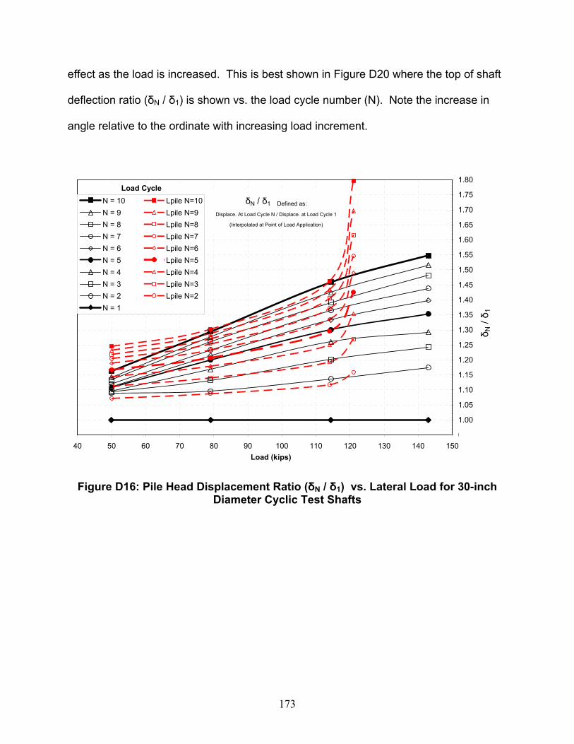
173
effect as the load is increased. This is best shown in Figure D20 where the top of shaft
deflection ratio (δN / δ1) is shown vs. the load cycle number (N). Note the increase in
angle relative to the ordinate with increasing load increment.
0.95
1.00
1.05
1.10
1.15
1.20
1.25
1.30
1.35
1.40
1.45
1.50
1.55
1.60
1.65
1.70
1.75
1.80
40 50 60 70 80 90 100 110 120 130 140 150Load (kips)
N = 10 Lpile N=10N = 9 Lpile N=9N = 8 Lpile N=8N = 7 Lpile N=7N = 6 Lpile N=6N = 5 Lpile N=5N = 4 Lpile N=4N = 3 Lpile N=3N = 2 Lpile N=2N = 1
δ N / δ 1
Load Cycle
δN / δ1 Defined as:
Displace. At Load Cycle N / Displace. at Load Cycle 1
(Interpolated at Point of Load Application)
Figure D16: Pile Head Displacement Ratio (δN / δ1) vs. Lateral Load for 30-inch Diameter Cyclic Test Shafts
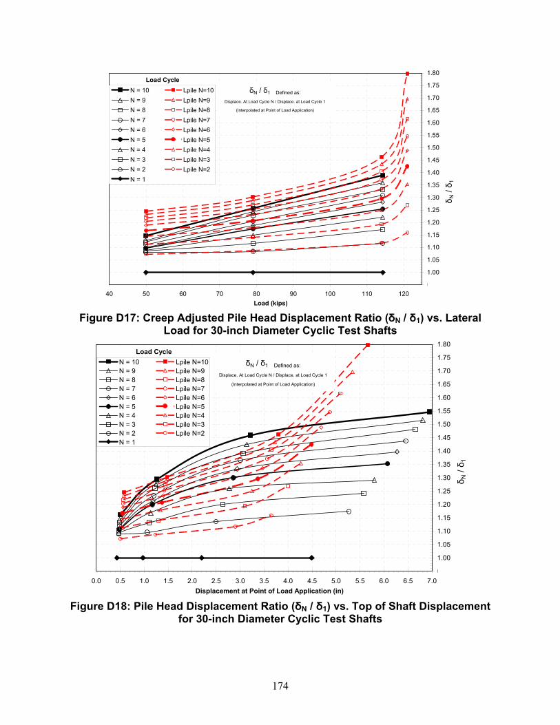
174
0.95
1.00
1.05
1.10
1.15
1.20
1.25
1.30
1.35
1.40
1.45
1.50
1.55
1.60
1.65
1.70
1.75
1.80
40 50 60 70 80 90 100 110 120Load (kips)
N = 10 Lpile N=10N = 9 Lpile N=9N = 8 Lpile N=8N = 7 Lpile N=7N = 6 Lpile N=6N = 5 Lpile N=5N = 4 Lpile N=4N = 3 Lpile N=3N = 2 Lpile N=2N = 1
δ N / δ 1
Load CycleδN / δ1 Defined as:
Displace. At Load Cycle N / Displace. at Load Cycle 1
(Interpolated at Point of Load Application)
Figure D17: Creep Adjusted Pile Head Displacement Ratio (δN / δ1) vs. Lateral
Load for 30-inch Diameter Cyclic Test Shafts
0.95
1.00
1.05
1.10
1.15
1.20
1.25
1.30
1.35
1.40
1.45
1.50
1.55
1.60
1.65
1.70
1.75
1.80
0.0 0.5 1.0 1.5 2.0 2.5 3.0 3.5 4.0 4.5 5.0 5.5 6.0 6.5 7.0Displacement at Point of Load Application (in)
N = 10 Lpile N=10N = 9 Lpile N=9N = 8 Lpile N=8N = 7 Lpile N=7N = 6 Lpile N=6N = 5 Lpile N=5N = 4 Lpile N=4N = 3 Lpile N=3N = 2 Lpile N=2N = 1
δ N / δ 1
Load Cycle
δN / δ1 Defined as:
Displace. At Load Cycle N / Displace. at Load Cycle 1
(Interpolated at Point of Load Application)
Figure D18: Pile Head Displacement Ratio (δN / δ1) vs. Top of Shaft Displacement
for 30-inch Diameter Cyclic Test Shafts

175
0.95
1.00
1.05
1.10
1.15
1.20
1.25
1.30
1.35
1.40
1.45
1.50
1.55
1.60
1.65
1.70
1.75
1.80
0.0 0.5 1.0 1.5 2.0 2.5 3.0 3.5 4.0 4.5 5.0 5.5 6.0Displacement at Point of Load Application (in)
N = 10 Lpile N=10N = 9 Lpile N=9N = 8 Lpile N=8N = 7 Lpile N=7N = 6 Lpile N=6N = 5 Lpile N=5N = 4 Lpile N=4N = 3 Lpile N=3N = 2 Lpile N=2N = 1
δ N / δ 1
Load CycleδN / δ1 Defined as:
Displace. At Load Cycle N / Displace. at Load Cycle 1
(Interpolated at Point of Load Application)
Figure D19: Creep Adjusted Pile Head Displacement Ratio (δN / δ1) vs. Top of
Shaft Displacement for 30-inch Diameter Cyclic Test Shafts
0.95
1.00
1.05
1.10
1.15
1.20
1.25
1.30
1.35
1.40
1.45
1.50
1.55
1 2 3 4 5 6 7 8 9 10Load Cycle (N)
Load Increment DLoad Increment C Creep Adjusted, CLoad Increment B Creep Adjusted, BLoad Increment A Creep Adjusted, A
δ N / δ 1
δN / δ1 Defined as:
Displace. At Load Cycle N / Displace. at Load Cycle 1
(Interpolated at Point of Load Application)
Figure D20: Pile Head Displacement Ratio (δN / δ1) vs. Load Cycle Number (N) for 30-inch Diameter Cyclic Test Shafts
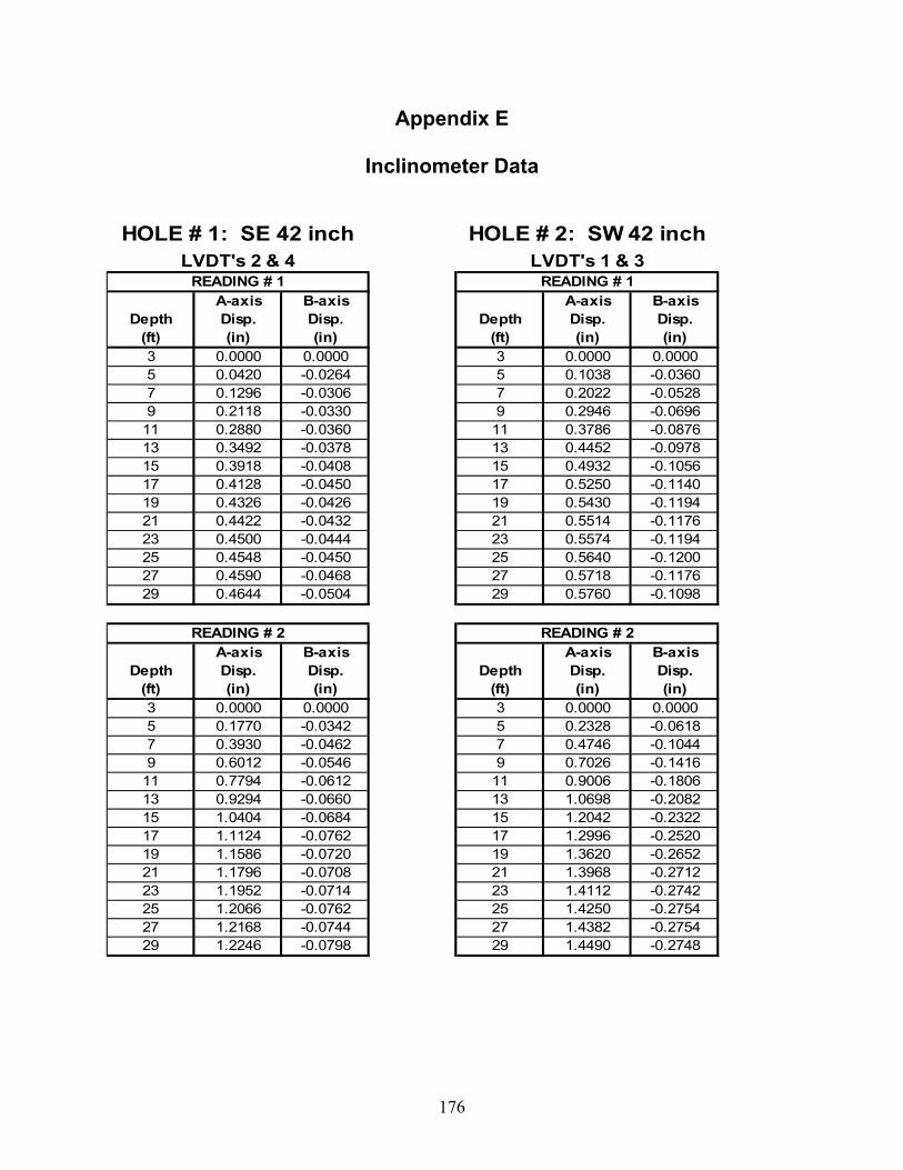
176
Appendix E
Inclinometer Data
HOLE # 1: SE 42 inch HOLE # 2: SW 42 inchLVDT's 2 & 4 LVDT's 1 & 3
READING # 1 READING # 1A-axis B-axis A-axis B-axis
Depth Disp. Disp. Depth Disp. Disp.(ft) (in) (in) (ft) (in) (in)3 0.0000 0.0000 3 0.0000 0.00005 0.0420 -0.0264 5 0.1038 -0.03607 0.1296 -0.0306 7 0.2022 -0.05289 0.2118 -0.0330 9 0.2946 -0.0696
11 0.2880 -0.0360 11 0.3786 -0.087613 0.3492 -0.0378 13 0.4452 -0.097815 0.3918 -0.0408 15 0.4932 -0.105617 0.4128 -0.0450 17 0.5250 -0.114019 0.4326 -0.0426 19 0.5430 -0.119421 0.4422 -0.0432 21 0.5514 -0.117623 0.4500 -0.0444 23 0.5574 -0.119425 0.4548 -0.0450 25 0.5640 -0.120027 0.4590 -0.0468 27 0.5718 -0.117629 0.4644 -0.0504 29 0.5760 -0.1098
READING # 2 READING # 2A-axis B-axis A-axis B-axis
Depth Disp. Disp. Depth Disp. Disp.(ft) (in) (in) (ft) (in) (in)3 0.0000 0.0000 3 0.0000 0.00005 0.1770 -0.0342 5 0.2328 -0.06187 0.3930 -0.0462 7 0.4746 -0.10449 0.6012 -0.0546 9 0.7026 -0.1416
11 0.7794 -0.0612 11 0.9006 -0.180613 0.9294 -0.0660 13 1.0698 -0.208215 1.0404 -0.0684 15 1.2042 -0.232217 1.1124 -0.0762 17 1.2996 -0.252019 1.1586 -0.0720 19 1.3620 -0.265221 1.1796 -0.0708 21 1.3968 -0.271223 1.1952 -0.0714 23 1.4112 -0.274225 1.2066 -0.0762 25 1.4250 -0.275427 1.2168 -0.0744 27 1.4382 -0.275429 1.2246 -0.0798 29 1.4490 -0.2748
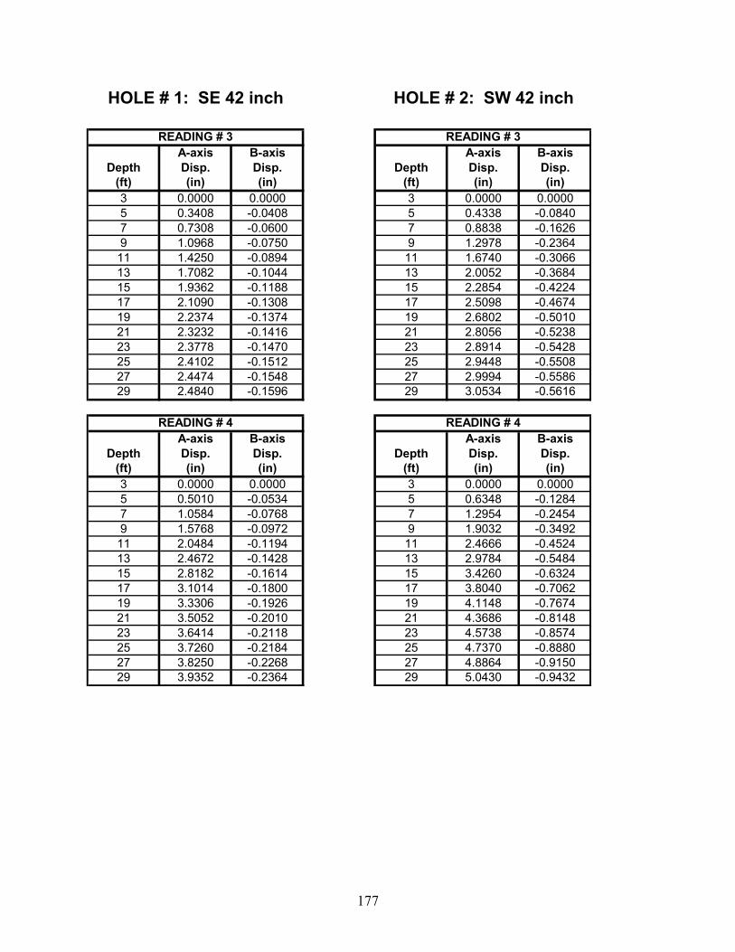
177
HOLE # 1: SE 42 inch HOLE # 2: SW 42 inch
READING # 3 READING # 3A-axis B-axis A-axis B-axis
Depth Disp. Disp. Depth Disp. Disp.(ft) (in) (in) (ft) (in) (in)3 0.0000 0.0000 3 0.0000 0.00005 0.3408 -0.0408 5 0.4338 -0.08407 0.7308 -0.0600 7 0.8838 -0.16269 1.0968 -0.0750 9 1.2978 -0.236411 1.4250 -0.0894 11 1.6740 -0.306613 1.7082 -0.1044 13 2.0052 -0.368415 1.9362 -0.1188 15 2.2854 -0.422417 2.1090 -0.1308 17 2.5098 -0.467419 2.2374 -0.1374 19 2.6802 -0.501021 2.3232 -0.1416 21 2.8056 -0.523823 2.3778 -0.1470 23 2.8914 -0.542825 2.4102 -0.1512 25 2.9448 -0.550827 2.4474 -0.1548 27 2.9994 -0.558629 2.4840 -0.1596 29 3.0534 -0.5616
READING # 4 READING # 4A-axis B-axis A-axis B-axis
Depth Disp. Disp. Depth Disp. Disp.(ft) (in) (in) (ft) (in) (in)3 0.0000 0.0000 3 0.0000 0.00005 0.5010 -0.0534 5 0.6348 -0.12847 1.0584 -0.0768 7 1.2954 -0.24549 1.5768 -0.0972 9 1.9032 -0.349211 2.0484 -0.1194 11 2.4666 -0.452413 2.4672 -0.1428 13 2.9784 -0.548415 2.8182 -0.1614 15 3.4260 -0.632417 3.1014 -0.1800 17 3.8040 -0.706219 3.3306 -0.1926 19 4.1148 -0.767421 3.5052 -0.2010 21 4.3686 -0.814823 3.6414 -0.2118 23 4.5738 -0.857425 3.7260 -0.2184 25 4.7370 -0.888027 3.8250 -0.2268 27 4.8864 -0.915029 3.9352 -0.2364 29 5.0430 -0.9432
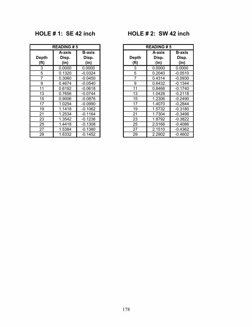
178
HOLE # 1: SE 42 inch HOLE # 2: SW 42 inch
READING # 5 READING # 5A-axis B-axis A-axis B-axis
Depth Disp. Disp. Depth Disp. Disp.(ft) (in) (in) (ft) (in) (in)3 0.0000 0.0000 3 0.0000 0.00005 0.1320 -0.0324 5 0.2040 -0.05107 0.3060 -0.0450 7 0.4314 -0.09309 0.4674 -0.0540 9 0.6432 -0.134411 0.6192 -0.0618 11 0.8466 -0.174013 0.7656 -0.0744 13 1.0428 -0.211815 0.9006 -0.0876 15 1.2306 -0.249017 1.0254 -0.0990 17 1.4070 -0.284419 1.1418 -0.1062 19 1.5732 -0.318021 1.2534 -0.1164 21 1.7304 -0.349823 1.3542 -0.1236 23 1.8792 -0.382225 1.4418 -0.1308 25 2.0166 -0.408627 1.5384 -0.1380 27 2.1510 -0.436229 1.6332 -0.1452 29 2.2902 -0.4602
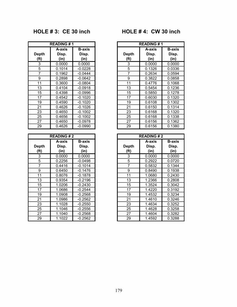
179
HOLE # 3: CE 30 inch HOLE # 4: CW 30 inch
READING # 1 READING # 1A-axis B-axis A-axis B-axis
Depth Disp. Disp. Depth Disp. Disp.(ft) (in) (in) (ft) (in) (in)3 0.0000 0.0000 3 0.0000 0.00005 0.1014 -0.0228 5 0.1326 0.03367 0.1962 -0.0444 7 0.2634 0.05949 0.2898 -0.0642 9 0.3822 0.085811 0.3600 -0.0804 11 0.4776 0.106813 0.4104 -0.0918 13 0.5454 0.123615 0.4398 -0.0996 15 0.5850 0.127817 0.4542 -0.1020 17 0.6030 0.132019 0.4590 -0.1020 19 0.6108 0.130221 0.4626 -0.1026 21 0.6150 0.131423 0.4650 -0.1002 23 0.6168 0.132025 0.4656 -0.1002 25 0.6168 0.133827 0.4650 -0.0978 27 0.6156 0.136229 0.4626 -0.0990 29 0.6156 0.1380
READING # 2 READING # 2A-axis B-axis A-axis B-axis
Depth Disp. Disp. Depth Disp. Disp.(ft) (in) (in) (ft) (in) (in)3 0.0000 0.0000 3 0.0000 0.00005 0.2256 -0.0498 5 0.2922 0.07207 0.4416 -0.1014 7 0.5832 0.13449 0.6450 -0.1476 9 0.8490 0.193811 0.8076 -0.1878 11 1.0680 0.243013 0.9354 -0.2196 13 1.2366 0.280815 1.0206 -0.2430 15 1.3524 0.304217 1.0686 -0.2544 17 1.4220 0.319219 1.0908 -0.2568 19 1.4532 0.323421 1.0986 -0.2562 21 1.4610 0.324623 1.1028 -0.2550 23 1.4634 0.325225 1.1046 -0.2556 25 1.4628 0.325827 1.1040 -0.2568 27 1.4604 0.328229 1.1022 -0.2562 29 1.4592 0.3288
180
HOLE # 3: CE 30 inch HOLE # 4: CW 30 inch
READING # 3 READING # 3A-axis B-axis A-axis B-axis
Depth Disp. Disp. Depth Disp. Disp.(ft) (in) (in) (ft) (in) (in)3 0.0000 0.0000 3 0.0000 0.00005 0.3744 -0.0876 5 0.4668 0.11467 0.7398 -0.1770 7 0.9342 0.21969 1.0824 -0.2568 9 1.3620 0.318011 1.3674 -0.3312 11 1.7250 0.402613 1.6008 -0.3918 13 2.0184 0.469815 1.7736 -0.4362 15 2.2344 0.518417 1.8882 -0.4638 17 2.3802 0.552019 1.9548 -0.4776 19 2.4612 0.564621 1.9848 -0.4842 21 2.4960 0.573623 1.9944 -0.4818 23 2.5044 0.576025 1.9974 -0.4830 25 2.5032 0.577827 1.9980 -0.4770 27 2.5026 0.578429 1.9962 -0.4758 29 2.5074 0.5712
READING # 4 READING # 4A-axis B-axis A-axis B-axis
Depth Disp. Disp. Depth Disp. Disp.(ft) (in) (in) (ft) (in) (in)3 0.0000 0.0000 3 0.0000 0.00005 0.7074 -0.1806 5 0.8784 0.22447 1.4118 -0.3576 7 1.7700 0.44169 2.0736 -0.5214 9 2.5896 0.645011 2.6556 -0.6762 11 3.3144 0.862813 3.1584 -0.8136 13 3.9186 0.979215 3.5574 -0.9234 15 4.3788 1.090217 3.8418 -1.0026 17 4.6950 1.165819 4.0302 -1.0542 19 4.8930 1.209021 4.1406 -1.0842 21 5.0052 1.237823 4.1934 -1.0920 23 5.0598 1.248625 4.2138 -1.0980 25 5.0748 1.251627 4.2288 -1.0986 27 5.0850 1.255229 4.2420 -1.0998 29 5.0952 1.2594
181
HOLE # 3: CE 30 inch HOLE # 4: CW 30 inch
READING # 5 READING # 5A-axis B-axis A-axis B-axis
Depth Disp. Disp. Depth Disp. Disp.(ft) (in) (in) (ft) (in) (in)3 0.0000 0.0000 3 0.0000 0.00005 0.1656 -0.0366 5 0.2250 0.06127 0.3294 -0.0750 7 0.4638 0.11769 0.4896 -0.1110 9 0.6852 0.175211 0.6324 -0.1440 11 0.8922 0.229813 0.7656 -0.1734 13 1.0788 0.278415 0.8802 -0.1998 15 1.2258 0.309017 0.9678 -0.2202 17 1.3290 0.334219 1.0344 -0.2340 19 1.4064 0.348021 1.0860 -0.2448 21 1.4640 0.363623 1.1214 -0.2496 23 1.5036 0.378625 1.1436 -0.2544 25 1.5240 0.387627 1.1658 -0.2568 27 1.5468 0.394229 1.1862 -0.2628 29 1.5756 0.3972
182
HOLE # 5: NE 30 inch HOLE # 6: NW 30 inch
READING # 1 READING # 1A-axis B-axis A-axis B-axis
Depth Disp. Disp. Depth Disp. Disp.(ft) (in) (in) (ft) (in) (in)3 0.0000 0.0000 3 0.0000 0.00005 0.0774 -0.0288 5 0.1386 -0.01267 0.1338 -0.0570 7 0.2718 -0.02349 0.1848 -0.0822 9 0.3900 -0.033611 0.2286 -0.1056 11 0.4818 -0.041413 0.2640 -0.1242 13 0.5472 -0.046815 0.2868 -0.1344 15 0.5892 -0.051617 0.2964 -0.1434 17 0.6114 -0.054019 0.3036 -0.1488 19 0.6216 -0.055821 0.3072 -0.1488 21 0.6276 -0.055223 0.3078 -0.1488 23 0.6312 -0.054025 0.3078 -0.1488 25 0.6378 -0.054627 0.3060 -0.1494 27 0.6324 -0.054629 0.3054 -0.1572 29 0.6324 -0.0552
READING # 2 READING # 2A-axis B-axis A-axis B-axis
Depth Disp. Disp. Depth Disp. Disp.(ft) (in) (in) (ft) (in) (in)3 0.0000 0.0000 3 0.0000 0.00005 0.1164 -0.0444 5 0.1374 -0.00907 0.2190 -0.0918 7 0.2730 -0.01929 0.3078 -0.1374 9 0.3936 -0.027611 0.3804 -0.1764 11 0.4914 -0.036613 0.4368 -0.2058 13 0.5646 -0.043215 0.4752 -0.2232 15 0.6162 -0.046817 0.4944 -0.2436 17 0.6426 -0.047419 0.5028 -0.2400 19 0.6552 -0.049221 0.5064 -0.2448 21 0.6636 -0.049823 0.5058 -0.2466 23 0.6672 -0.050425 0.5052 -0.2478 25 0.6672 -0.051627 0.5010 -0.2496 27 0.6672 -0.051029 0.5004 -0.2538 29 0.6678 -0.0510
183
READING # 3 READING # 3A-axis B-axis A-axis B-axis
Depth Disp. Disp. Depth Disp. Disp.(ft) (in) (in) (ft) (in) (in)3 0.0000 0.0000 3 0.0000 0.00005 0.2016 -0.0894 5 0.2250 -0.02107 0.3924 -0.1836 7 0.5052 -0.03909 0.5658 -0.2700 9 0.7320 -0.055211 0.7080 -0.3426 11 0.9186 -0.069613 0.8178 -0.4002 13 1.0650 -0.081015 0.8916 -0.4386 15 1.1694 -0.088817 0.9342 -0.4614 17 1.2330 -0.094219 0.9516 -0.4716 19 1.2648 -0.098421 0.9606 -0.4764 21 1.2774 -0.099623 0.9630 -0.4788 23 1.2828 -0.101425 0.9642 -0.4800 25 1.2840 -0.101427 0.9630 -0.4824 27 1.2840 -0.101429 0.9624 -0.4878 29 1.2834 -0.1032
READING # 4 READING # 4A-axis B-axis A-axis B-axis
Depth Disp. Disp. Depth Disp. Disp.(ft) (in) (in) (ft) (in) (in)3 0.0000 0.0000 3 0.0000 0.00005 0.2484 -0.1074 5 0.3036 -0.02287 0.4788 -0.2214 7 0.6054 -0.04449 0.6936 -0.3252 9 0.8802 -0.062411 0.8772 -0.4164 11 1.1188 -0.080413 1.0242 -0.4926 13 1.2984 -0.094815 1.1286 -0.5466 15 1.4376 -0.105017 1.1958 -0.5832 17 1.5312 -0.111019 1.2336 -0.6048 19 1.5852 -0.114021 1.2462 -0.6150 21 1.6110 -0.115823 1.2516 -0.6174 23 1.6212 -0.117625 1.2540 -0.6198 25 1.6254 -0.117627 1.2552 -0.5234 27 1.6284 -0.117629 1.2552 -0.6294 29 1.6314 -0.1176
184
READING # 5 READING # 5A-axis B-axis A-axis B-axis
Depth Disp. Disp. Depth Disp. Disp.(ft) (in) (in) (ft) (in) (in)3 0.0000 0.0000 3 0.0000 0.00005 0.4122 -0.1884 5 0.4962 -0.02887 0.8142 -0.3834 7 0.9852 -0.06009 1.1832 -0.5622 9 1.4352 -0.087611 1.5036 -0.7224 11 1.8228 -0.115813 1.7694 -0.8568 13 2.1444 -0.140415 1.9698 -0.9588 15 2.3946 -0.156617 2.1078 -1.0326 17 2.5746 -0.166819 2.1924 -1.0776 19 2.6868 -0.172821 2.2314 -1.1034 21 2.7492 -0.174023 2.2440 -1.1076 23 2.7738 -0.176425 2.2506 -1.1106 25 2.7804 -0.177627 2.2530 -1.1142 27 2.7852 -0.176429 2.2536 -1.1190 29 2.7888 -0.1716
READING # 6 READING # 6A-axis B-axis A-axis B-axis
Depth Disp. Disp. Depth Disp. Disp.(ft) (in) (in) (ft) (in) (in)3 0.0000 0.0000 3 0.0000 0.00005 0.5184 -0.2412 5 0.6498 -0.03247 1.0362 -0.4974 7 1.2906 -0.06729 1.5174 -0.7338 9 1.8840 -0.100811 1.9446 -0.9540 11 2.4108 -0.133213 2.3100 -1.1454 13 2.8578 -0.162015 2.5998 -1.2972 15 3.2220 -0.181817 2.8170 -1.4136 17 3.5052 -0.195019 2.9652 -1.4934 19 3.7050 -0.202821 3.0540 -1.5456 21 3.8352 -0.206423 3.1014 -1.5702 23 3.9132 -0.208225 3.1200 -1.5822 25 3.9540 -0.207627 3.1356 -1.5918 27 3.9906 -0.204629 3.1494 -1.6032 29 4.0260 -0.2022
185
READING # 7 READING # 7A-axis B-axis A-axis B-axis
Depth Disp. Disp. Depth Disp. Disp.(ft) (in) (in) (ft) (in) (in)3 0.0000 0.0000 3 0.0000 0.00005 0.7542 -0.3582 5 0.9780 -0.04927 1.5132 -0.7314 7 1.9398 -0.09969 2.2248 -1.0794 9 2.8398 -0.152411 2.8668 -1.4070 11 3.6516 -0.204613 3.4254 -1.6962 13 4.3440 -0.252615 3.8658 -1.9254 15 4.8954 -0.283817 4.1808 -2.0940 17 5.3022 -0.302419 4.3890 -2.2056 19 5.5800 -0.313821 4.5162 -2.2788 21 5.7600 -0.320423 4.5852 -2.3130 23 5.8716 -0.325825 4.6170 -2.3310 25 5.9316 -0.327627 4.6338 -2.3436 27 5.9790 -0.325229 4.6518 -2.3610 29 6.0270 -0.3216
READING # 8 READING # 8A-axis B-axis A-axis B-axis
Depth Disp. Disp. Depth Disp. Disp.(ft) (in) (in) (ft) (in) (in)3 0.0000 0.0000 3 0.0000 0.00005 1.0404 -0.5070 5 1.3080 -0.05407 2.0994 -1.0332 7 2.5920 -0.10929 3.1074 -1.5378 9 3.8130 -0.170411 4.0398 -2.0148 11 4.9338 -0.231613 4.8756 -2.4540 13 5.9196 -0.284415 5.5572 -2.8116 15 6.7230 -0.318017 6.0588 -3.0816 17 7.3308 -0.337819 6.4098 -3.2682 19 7.7724 -0.349821 6.6570 -3.4074 21 8.1018 -0.356423 6.8346 -3.5028 23 8.3520 -0.361825 6.9600 -3.5718 25 8.5380 -0.358827 7.0572 -3.6312 27 8.7054 -0.354029 7.1598 -3.6984 29 8.8758 -0.3492
186
READING # 9 READING # 9A-axis B-axis A-axis B-axis
Depth Disp. Disp. Depth Disp. Disp.(ft) (in) (in) (ft) (in) (in)3 0.0000 0.0000 3 0.0000 0.00005 0.2328 -0.1140 5 0.3300 -0.00727 0.4692 0.2394 7 0.6540 -0.01629 0.6960 -0.3612 9 0.9696 -0.027611 0.9126 -0.4806 11 1.2732 -0.040813 1.1184 -0.5964 13 1.5462 -0.052215 1.2780 -0.6876 15 1.7622 -0.055217 1.3752 -0.7476 17 1.9098 -0.051019 1.4304 -0.7836 19 2.0142 -0.044421 1.4754 -0.8154 21 2.1096 -0.035423 1.5180 -0.8424 23 2.2038 -0.027025 1.5576 -0.8700 25 2.2944 -0.020427 1.5972 -0.8994 27 2.3850 -0.012629 1.6410 -0.9306 29 2.4774 -0.0060