Soil and Water Assessment Tool, Gediz â€“ Turkey - FutureWater

Soil and Water Assessment Tool,

Gediz – Turkey

WatManSup project

WatManSup Report No 6

2007 WatManSup Report No. 6

Soil and Water Assessment Tool, Gediz Basin - Turkey

WatManSup Report No 6

Authors:

Peter Droogers (FutureWater)

Anne van Loon (FutureWater)

FutureWater

Costerweg 1G

6702 AA Wageningen

Netherlands

tel: +31 (0)317 460050

email: [email protected]

web: www.futurewater.nl

1/30

WatManSup Report No. 6 2007

Preface

This report is written in the context of the WatManSup project (Integrated Water Management Support

Methodologies). The project is executed in two countries: Kenya and Turkey. Financial support is

provided by Partners for Water. For more information on the WatManSup project see the project

website: http://www.futurewater.nl/watmansup.

The Dutch consortium: FutureWater (Wageningen)

Institute for Environmental Studies (Amsterdam)

Water Board Hunze en Aa's (Veendam)

Foreign clients: SASOL Foundation (Kitui, Kenya)

Soil and Water Resources Research Institutes of the Turkish Ministry of Agricultural and Rural Affairs

(Menemen, Turkey)

SUMER (Izmir, Turkey)

Additional technical support: the University of Nairobi (Kenya)

EA-TEK (Izmir, Turkey)

Reports so far: Report No.1: Water Management Support Methodologies: State of the Art

Report No.2: Water Evaluation and Planning System, Kitui - Kenya

Report No.3: Soil and Water Assessment Tool, Kitui - Kenya

Report No.4: Multi-criteria analysis, Kitui - Kenya

Report No.5: Water Evaluation and Planning System, Gediz Basin - Turkey

Report No.6: Soil and Water Assessment Tool, Gediz Basin - Turkey

2/30


Table of Contents 1 INTRODUCTION 5

2 METHODS AND STUDY AREA 7 2.1 SWAT model 7 2.2 Gediz Basin, Turkey 9

3 SETTING-UP SWAT 11 3.1 Watershed delineation 11 3.2 Land use 12 3.3 Soils 14 3.4 Hydrological Response Units 14 3.5 Irrigation and Reservoirs 15

4 CALIBRATION 17

5 RESULTS 19 5.1 Output generation 19 5.2 Stream flow 20 5.3 Detailed soil water balances 21 5.4 Spatially distributed results 23

6 CONCLUSIONS 27

REFERENCES 29

3/30


Tables Table 1. Land cover classes included in the model. ............................................................................................ 13 Table 2. Stream flow at four locations in Gediz (see Figure 8). All data in m3 s-1. ................................................. 20

Figures Figure 1. Main land phase processes as implemented within SWAT....................................................................... 7 Figure 2. Schematic diagram of the sub-surface water fluxes. .............................................................................. 8 Figure 3. Parameterisation of crop production. .................................................................................................... 8 Figure 4: Location of Gediz Basin in Turkey. ........................................................................................................ 9 Figure 5. Elevation data for Western Turkey based on HYDRO1K........................................................................ 11 Figure 6. Final layout of streams and sub-catchments. ....................................................................................... 12 Figure 7. Land cover data (top original, bottom translated to SWAT classes). ...................................................... 13 Figure 8. Distribution of the five soil classes included in the SWAT model for Gediz Basin..................................... 14 Figure 9. Hydrological Response Units (HRUs) distinguished in the Basin. ........................................................... 15 Figure 10. Example input screen for crop characteristics in SWAT....................................................................... 17 Figure 11. Calibration for HRU 80 (AGRL, FAO3139) for 1992. Red line is simulated Leaf Area Index and

green line is simulated biomass. ................................................................................................................ 18 Figure 12. Refinement of crop growth for mixed forest (HRU 63, FRST, FAO3114) with Scheduled by Date

1 Jan - 31 Dec. Total Heat Units 3000 (top) and 3500 (bottom). ................................................................. 18 Figure 13. Example of output evaluation in the AVSWAT interface. ..................................................................... 19 Figure 14. Daily stream flow for three locations in Gediz. ................................................................................... 21 Figure 15. Daily stream flow and storage for Demirköprü reservoir (maximum storage = 1300 MCM). .................. 21 Figure 16. Potential and actual evapotranspiration for one HRU (Irrigated Agriculture, HRU 132).......................... 22 Figure 17. Cumulative daily water balance for one HRU (Irrigated Agriculture, HRU 132). .................................... 23 Figure 18. Storage in the three soil components (Irrigated Agriculture, HRU 132)................................................ 23 Figure 19. Actual evapotranspiration (ET) in 1993.............................................................................................. 24 Figure 20. Water yield contributing to stream flow in 1993................................................................................. 24 Figure 21. Surface runoff in 1993. .................................................................................................................... 25 Figure 22. Groundwater runoff in 1993. ............................................................................................................ 25

4/30


1 Introduction The challenge to manage our water resources in a sustainable and appropriate manner is growing.

Water related disasters are not accepted anymore and societies expect more and more that water is

always available at the right moment and at the desired quantity and quality. Current water

management practices are still focused on reacting to events occurred in the past: the re-active

approach. At many international high level ministerial and scientific meetings a call for more strategic

oriented water management, the pro-active approach, has been advocated. Despite these calls such a

pro-active approach is hardly adopted by water managers and policy makers. One of the main reasons

for this slow adoption is the lack of appropriate tools.

To be prepared for the paradigm shift, from a re-active towards a pro-active approach, Integrated

Water Management Support Methodologies (IWMSM) are needed that go beyond the traditional

operational support tools. Note that these IWMSM are more than only tools, but include conceptual

issues, theories, combining technical and socio-economic aspects. To demonstrate and promote this

new way of thinking the WatManSup project (Water Management Support Tools) has been initiated.

The IWMSM approach comprises three different components: a water allocation component, a physical

based component and a decision support component. This report demonstrates how the physical

based component can be developed for one of the study areas included in the WatManSup project:

Gediz Basin in Turkey.

The overall objective of this report is to demonstrate in which way the physical based component of

IWMSM, the SWAT tool, can be used to support water managers and policy makers in a setting where

irrigation is the dominant user of allocated water.

5/30


6/30


2 Methods and study area

2.1 SWAT model SWAT is the acronym for Soil and Water Assessment Tool, a river basin model developed originally by

the USDA Agricultural Research Service (ARS) and Texas A&M University, that is currently one of the

worlds leading spatially distributed hydrological models. SWAT has been used extensively by

FutureWater in various places and important modifications, improvements and extensions have been

developed.

A distributed rainfall-runoff model – such as SWAT – divides a catchment into smaller discrete

calculation units for which the spatial variation of the major physical properties are limited, and

hydrological processes can be treated as being homogeneous. The total catchment behaviour is a net

result of manifold small sub-basins. The soil map and land cover map within sub-basin boundaries are

used to generate unique combinations, and each combination will be considered as a homogeneous

physical property, i.e. Hydrological Response Unit (HRU). The water balance for HRUs is computed on

a daily time step. Hence, SWAT will subdivide the river basin into units that have similar characteristics

in soil and land cover and that are located in the same sub-basin.

Irrigation in SWAT can be scheduled by the user or automatically determined by the model depending

on a set of criteria. In addition to specifying the timing and application amount, the source of irrigation

water must be specified, which can be: canal water, reservoir, shallow aquifer, deep aquifer, or a

source outside the basin.

Root Zone

Shallow (unconfined)

Aquifer

Vadose(unsaturated)

Zone

Confining Layer

Deep (confined) Aquifer

Evaporation and Transpiration

Infiltration/plant uptake/ Soil moisture redistribution

Lateral Flow

Surface Runoff

Precipitation

Return Flow

Revap from shallow aquifer

Percolation to shallow aquifer

Recharge to deep aquifer

Flow out of watershed

Figure 1. Main land phase processes as implemented within SWAT.

SWAT can deal with standard groundwater processes (Figure 1). Water enters groundwater storage

primarily by infiltration/percolation, although recharge by seepage from surface water bodies is also

included. Water leaves groundwater storage primarily by discharge into rivers or lakes, but it is also

possible for water to move upward from the water table into the capillary fringe, i.e. capillary rise. As

7/30


mentioned before, water can also be extracted by mankind for irrigation purposes. SWAT distinguishes

recharge and discharge zones.

Recharge to unconfined aquifers occurs via percolation of excessively wet root zones. Recharge to

confined aquifers by percolation from the surface occurs only at the upstream end of the confined

aquifer, where the geologic formation containing the aquifer is exposed at the earth’s surface, flow is

not confined, and a water table is present. Irrigation and link canals can be connected to the

groundwater system; this can be an effluent as well as an influent stream.

After water is infiltrated into the soil, it can basically leave the ground again as lateral flow from the

upper soil layer – which mimics a 2D flow domain in the unsaturated zone – or as return flow that

leaves the shallow aquifer and drains into a nearby river (Figure 2). The remaining part of the soil

moisture can feed into the deep aquifer, from which it can be pumped back. The total return flow thus

consists of surface runoff, lateral outflow from root zone and aquifer drainage to river.

Figure 2. Schematic diagram of the sub-surface water fluxes.

Figure 3. Parameterisation of crop production.

For each day of simulation, potential plant growth, i.e. plant growth under ideal growing conditions is

calculated. Ideal growing conditions consist of adequate water and nutrient supply and a favourable

8/30


climate. First, the Absorbed Photosynthetical Radiation (APAR) is computed from intercepted solar

radiation, followed by a Light Use Efficiency (LUE) that in SWAT is essentially a function of carbon

dioxide concentrations and vapour pressure deficits. The crop yield is computed as the harvestable

fraction of the accumulated biomass production across the growing season (Figure 3).

Details of the SWAT model can be found at various background material (e.g. Neitsch, 2002a; Neitsch,

2002b). Examples of practical application can be found elsewhere (SWAT, 2007; FutureWater, 2007).

2.2 Gediz Basin, Turkey Gediz Basin is located in the western part of Turkey, just north of Izmir. Gediz river flows from east to

west into the Aegean Sea, is about 275 km long and drains an area of 17,200 km2 (DSI, 2006). In

Gediz Basin water scarcity is a significant problem due to competition for water among various uses

(water allocation problems). Most conflicts arise between irrigation with a total command area of

110,000 ha, and the domestic and (fast growing) industrial demand in the coastal zone. Another

problem is environmental pollution. The basin experiences droughts from time to time. Water use in

the 90,000 ha irrigated agriculture of the central and delta zones is limited to 75 m3 s-1 from

Demirköprü reservoir and 15 m3 s-1 from Göl Marmara for a release period of approximately 60 days,

or a total of some 550 million cubic meters (MCM) during the year. This is equivalent to some 450 mm

of irrigation water for the growing season. There are serious institutional, legal, social and economic

drawbacks, which enhance water allocation and environmental pollution problems. In this study we

focus on the physical processes included in SWAT to deal with water demand as well as supply in all

areas and land covers in the basin.

More details about Gediz Basin and its challenges can be found in various other publications (SMART,

2007; Kite and Droogers, 1999; THAEM, 1999; WatManSup, 2007)

Figure 4: Location of Gediz Basin in Turkey.

Gediz Basin

9/30


10/30


3 Setting-up SWAT

3.1 Watershed delineation First step required to build a SWAT model is defining the elevation related properties such as: elevation

above sea level, slope, aspect, stream flow network, and distance to nearest stream, and dividing the

basin in sub-catchments. The HYDRO1K (USGS, 2006) dataset was used for this and a clipped portion

for Western Turkey is shown in Figure 5.

Figure 5. Elevation data for Western Turkey based on HYDRO1K.

Within SWAT one can define the number of sub-catchment to be included in the study, based on a

minimum area of each sub-catchment. There is no optimal number of sub-catchments as it depends on

the question to be answered, as well as time, resources and data availability. Given the nature of this

demonstration case, an appropriate threshold value is somewhere between 10,000 and 50,000 ha. A

lower value provided too much detail in the flat areas, while a higher value resulted in sub-catchments

that were too large in the mountainous areas. Optimal sizes of sub-catchments were obtained by using

a threshold value of 50,000 ha and manually adding more details in the mountainous areas, resulting

in 49 sub-catchments. The final layout can be seen in Figure 6.

11/30


Figure 6. Final layout of streams and sub-catchments.

3.2 Land use The type of vegetation determines many components of the hydrological cycle: total water

requirement, irrigation demand, actual water consumption by evapotranspiration, surface runoff,

percolation, and erosion. SWAT includes a detailed crop growth module which is based on the EPIC

crop model (Williams et al., 1984). SWAT uses EPIC concepts of phenological crop development based

on daily accumulated heat units, harvest index for partitioning grain yield, Monteith’s approach

(Monteith, 1977) for potential biomass, and water and temperature stress adjustments.

The number of vegetation types and crops that can be included in SWAT is virtually unlimited. For

practical reasons it is important that the level of detail is in correspondence with the question to be

answered during the modelling. Since the objective of this study is demonstration oriented, it was

decided to use a simplified land cover map including seven classes. This land cover map was prepared

using NOAA satellite information, a unsupervised classification method, combined with post-

classification field verification. Details of this approach can be found elsewhere (Droogers et al., 1999).

The classes of the original land cover map were translated to standard SWAT classes (Table 1 and

Figure 7).

12/30


Table 1. Land cover classes included in the model.

Land cover Internal code SWAT classes

Other 0 FRST

Water bodies 1 WATR

Maki 2 FRST

Coniferous 3 FRSE

Non-irrigated 4 AGRL

Irrigated 5 AGRI

Barren 6 RNGE

Shrubland 7 RNGB

TIRE

URLABUCA

KULA

USAK

IZMIR

KINIK

BULDAN

ODEMIS

CIVRIL

MANISA

OVAKENT

BORNOVA

SALIHLIURGANLI

MENEMEN

AKHISAR

DEMIRCIBERGAMA

ALASEHIR

TURGUTLU

KIRKAGAC

ALTINOVA

SARUHANLI

Land use

Water

Maki

Coniferous

Agriculture

Irrigated

Barren

Shrubland

Gediz SWATWatManSup

0 25 5012.5 km

Figure 7. Land cover data (top original, bottom translated to SWAT classes).

13/30


3.3 Soils Soils are the determining factors for hydrological processes such as: surface runoff, infiltration,

percolation, lateral subsurface flow, plant water availability, etc. Since no detailed soil map was readily

accessible for Gediz Basin, the FAO Soils of the World (FAO, 2000) data were used. The FAO dataset

includes only qualitative descriptions, while for SWAT quantitative soil physical characteristics are

required. For this demonstration case a simple transfer was used based on previous experiences with

SWAT (Kauffman and Droogers, 2007; Immerzeel and Droogers, 2007; Van Loon and Droogers, 2007).

The final soil data set included five classes and is shown in Figure 8.

Figure 8. Distribution of the five soil classes included in the SWAT model for Gediz Basin.

3.4 Hydrological Response Units A specific characteristic of the SWAT model is the subdivision of the study area in so-called

Hydrological Response Units (HRUs). These HRUs form unique combinations of a specific soil type and

land cover type within a sub-catchment. One can specify the number of HRUs required in a sub-

catchment based on a threshold value, which is the area percentage of land cover and soils in a sub-

catchment that can be neglected. Smaller threshold values will result in more detail. Given the nature

of this demonstration case and the importance of land cover a threshold value of 5% was used for

land cover and 20% for soils. Using these threshold values a total of 255 HRUs was distinguished in

the basin (Figure 9).

14/30


Figure 9. Hydrological Response Units (HRUs) distinguished in the Basin.

0 25 5012.5 km

3.5 Irrigation and Reservoirs SWAT includes a module for auto-irrigation where the source of water should be specified. A total of

five different sources can be specified: canal water, reservoir, shallow aquifer, deep aquifer, or a

source outside the basin. In the current model three reservoirs have been included: Göl Marmara,

Demirköprü and the combined Afsar and Buldan as one representative reservoir. Most large irrigation

schemes receive water from these reservoirs, while some upstream irrigation fields are considered to

receive water from groundwater.

15/30


16/30


4 Calibration A full calibration was not performed as the objectives of this study were to demonstrate the

opportunities SWAT offers to evaluate water resources in the basin and to assist water managers and

decision makers in their responsibilities. However, land cover is one of the dominant features

characterising the hydrological behaviour of an area. Moreover, the standard land cover characteristics

included in SWAT are all based on conditions in USA and are therefore not necessarily valid for Turkey.

Therefore, a basic calibration based on expert knowledge was performed on land cover.

Figure 10 shows the input screen in SWAT where part of the growing characteristics of a vegetation

type or crop are determined. In the calibration process these parameters can be adjusted. As an

example of the calibration procedure followed, Figure 11 shows four steps taken during calibration of

one specific crop type. The example shows the land cover type Agriculture Generic for one specific soil

type, in one specific sub-catchment. By varying the total Heat Units required to harvest between 1500

and 3000, and simultaneously changing the fractions to reach the first growing point (FRGRW1) and

the last growing point (FRGRW2) a more realistic growing pattern was obtained. In Figure 11 the

following parameter values were used:

• A: Heat Units: 1500; FRGRW1: 0.15; FRGRW2: 1.20

• B: Heat Units: 2000; FRGRW1: 0.15; FRGRW2: 1.20

• C: Heat Units: 2500; FRGRW1: 0.15; FRGRW2: 1.20

• D: Heat Units: 3000; FRGRW1: 0.10; FRGRW2: 1.00

As a second example, the calibration of a permanent vegetation type (mixed forest) is presented in

Figure 12. Here, the total Heat Units were changed from 3000 to 3500 to lengthen the growing season

to obtain a more realistic LAI (Leaf Area Index) graph for the case in Gediz. Note that this mixed forest

has year-round green vegetation, with some enhanced green development during spring and leaf

senescence during autumn.

Figure 10. Example input screen for crop characteristics in SWAT.

17/30


A

0.0

0.1

0.2

0.3

0.4

0.5

0.6

0.7

0.8

0.9

1.0

01-J

an

01-F

eb

01-M

ar

01-A

pr

01-M

ay

01-J

un

01-J

ul

01-A

ug

01-S

ep

01-O

ct

01-N

ov

01-D

ec

LAI (

m2 m

-2)

0

50

100

150

200

250

Bio

mas

s (to

n ha

-1)

LAIBiomassBiomassAvg

B

0.0

0.1

0.2

0.3

0.4

0.5

0.6

0.7

0.8

0.9

01-J

an

01-F

eb

01-M

ar

01-A

pr

01-M

ay

01-J

un

01-J

ul

01-A

ug

01-S

ep

01-O

ct

01-N

ov

01-D

ec

LAI (

m2 m

-2)

0

20

40

60

80

100

120

140

160

180

200

Bio

mas

s (to

n ha

-1)


C

0.0

0.1

0.2

0.3

0.4

0.5

0.6

0.7

0.8

0.9

01-J

an

01-F

eb

01-M

ar

01-A

pr

01-M

ay

01-J

un

01-J

ul

01-A

ug

01-S

ep

01-O

ct

01-N

ov

01-D

ec

LAI (

m2 m

-2)

0

20

40

60

80

100

120

140

160

180

200

Bio

mas

s (to

n ha

-1)


D

0.0

0.1

0.2

0.3

0.4

0.5

0.6

0.7

0.8

0.9

01-J

an

01-F

eb

01-M

ar

01-A

pr

01-M

ay

01-J

un

01-J

ul

01-A

ug

01-S

ep

01-O

ct

01-N

ov

01-D

ec

LAI (

m2 m

-2)

0

20

40

60

80

100

120

140

160

180

200

Bio

mas

s (to

n ha

-1)


Figure 11. Calibration for HRU 80 (AGRL, FAO3139) for 1992. Red line is simulated Leaf Area Index and green line is simulated biomass.

0.0

0.5

1.0

1.5

2.0

2.5

3.0

3.5

4.0

4.5

5.0

01-J

an

01-F

eb

01-M

ar

01-A

pr

01-M

ay

01-J

un

01-J

ul

01-A

ug

01-S

ep

01-O

ct

01-N

ov

01-D

ec

LAI (

m2 m

-2)

0

20

40

60

80

100

120

140

160

180

200

Bio

mas

s (to

n ha

-1)


0.0

0.5

1.0

1.5

2.0

2.5

3.0

3.5

4.0

4.5

5.0

01-J

an

01-F

eb

01-M

ar

01-A

pr

01-M

ay

01-J

un

01-J

ul

01-A

ug

01-S

ep

01-O

ct

01-N

ov

01-D

ec

LAI (

m2 m

-2)

0

20

40

60

80

100

120

140

160

180

200

Bio

mas

s (to

n ha

-1)


Figure 12. Refinement of crop growth for mixed forest (HRU 63, FRST, FAO3114) with Scheduled by Date 1 Jan - 31 Dec. Total Heat Units 3000 (top) and 3500 (bottom).

18/30


5 Results

5.1 Output generation The model as developed for Gediz Basin and described in the previous sections is used to demonstrate

the types of output that can be generated by SWAT. As emphasised earlier, the objective of the

project was to demonstrate the opportunities SWAT offers to support decision makers and water

managers, rather than to develop a complete calibrated model for the basin. Results presented here

therefore do not reflect actual conditions.

Figure 13 provides an example of the option to analyse output using the AVSWAT interface. Tables,

graphs and maps are generated and can be customised to a certain extent. One of the missing aspects

in the AVSWAT interface is however that output can be generated only at the level of sub-catchments,

in stead of at the much more relevant HRU level. Especially in areas like Gediz, where relatively large

spatial differences exist, important details cannot be displayed and evaluated in the standard AVSWAT

interface. A typical example of this is crop production and actual evapotranspiration differences

between irrigated and non-irrigated crops. To overcome these problems a GIS tool was developed to

evaluate output at HRU level (Immerzeel and Droogers, 2007).

Figure 13. Example of output evaluation in the AVSWAT interface.

Output generated by SWAT is huge and sometimes somewhat overwhelming. One can select to have

output written per day, month or year. Moreover, output files include results for the entire basin, for

each sub-catchment and for each HRU. In addition, stream flow is provided for each sub-catchment

and details on reservoir inflow, outflow and storage are given as well. Crop growth output, such as

19/30


LAI, biomass production, water and nutrient stress, and erosion are generated. Finally, all kind of

output related to water quality can be evaluated.

In general, three different types of output are being generated by the SWAT model: (i) stream flow in

channels, (ii) detailed soil water balances, (iii) spatially distributed output. Of each of these output

types typical examples will be presented hereafter.

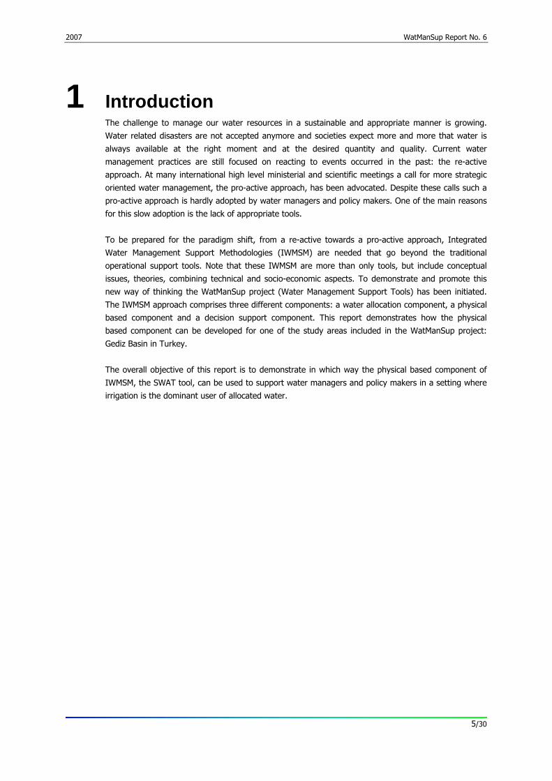
5.2 Stream flow SWAT generates stream flow for each point in the basin at daily, monthly and annual interval. This

data can be plotted using the AVSWAT interface, or exported and plotted with other software

packages. As an example, Table 2 shows the average annual stream flow at four locations in Gediz

Basin. These flows are higher than observed ones (see Kite and Droogers, 1999), which can be

explained by the lack of good quality input data. Moreover, detailed calibration can improve the stream

flow results considerably. In this preliminary study such a calibration has not been performed yet (see

Section 4).

SWAT offers detailed output to enable evaluation of water resources and improvement of model

performance if required. As an example Figure 14 shows stream flow at a daily interval for three

locations in Gediz, upstream, middle and downstream, indicating some high peak flows downstream.

In reality, peak flows are rare in downstream parts of the basin as Demirköprü stores peak runoffs

from upper parts of the basin. Further analysis (Figure 15) shows the daily inflows, outflows and

storage of Demirköprü reservoir. In the current SWAT model the reservoir is always full during

wintertime, causing severe downstream flooding from winter and spring rains, that top the emergency

spillway of the reservoir.

Further analysis, as presented in following paragraphs, indicates that the obtained soil data were not

correct: permeability was too low, resulting in low percolation rates and therefore high surface runoffs.

Also, storage capacity of the shallow aquifer as represented in the current model seems lower than in

reality. This also reduces the amount of water stored in the soil profile, resulting in too low actual

evapotranspiration rates during summers. Model refinement and calibration should therefore be

undertaken before the model can be applied to real problem solving in Gediz Basin.

Table 2. Stream flow at four locations in Gediz (see Figure 8). All data in m3 s-1.

Sub-catchment 36 37 26 33 Location Gediz Alasehir Kumcay Outflow

1992 12 2 10 18 1993 45 15 36 91 1994 39 11 27 77 1995 56 13 51 133 1996 45 12 33 97 Aver 39 11 32 83

20/30


0

100

200

300

400

500

600

700

800

900

1000

01/0

1/19

92

01/0

5/19

92

01/0

9/19

92

01/0

1/19

93

01/0

5/19

93

01/0

9/19

93

01/0

1/19

94

01/0

5/19

94

01/0

9/19

94

01/0

1/19

95

01/0

5/19

95

01/0

9/19

95

01/0

1/19

96

01/0

5/19

96

01/0

9/19

96

Flow

s (m

3/s)

MiddleDownstreamUpstream

Figure 14. Daily stream flow for three locations in Gediz.

0

50

100

150

200

250

300

01/0

1/19

9201

/04/

1992

01/0

7/19

9201

/10/

1992

01/0

1/19

9301

/04/

1993

01/0

7/19

9301

/10/

1993

01/0

1/19

9401

/04/

1994

01/0

7/19

9401

/10/

1994

01/0

1/19

9501

/04/

1995

01/0

7/19

9501

/10/

1995

01/0

1/19

9601

/04/

1996

01/0

7/19

9601

/10/

1996

Flow

s (m

3/s)

-100

100

300

500

700

900

1100

1300

1500

1700

Volu

me

(MC

M)

InOutVolume

Figure 15. Daily stream flow and storage for Demirköprü reservoir (maximum storage = 1300 MCM).

5.3 Detailed soil water balances Output per HRU is written to the so-called SBS file. File size can be enormous if output is written per

day. For the Gediz case (255 HRUs, five years) a file of 300 MB is generated and special software has

been developed during the project to extract specific information from the file. This software can be

used to extract a particular HRU and/or a specific year, which can than be used by any plotting

program.

21/30


As an example to demonstrate the opportunities SWAT offers to analyse processes in detail, Figure 16

shows daily potential and actual evapotranspiration (ET) for one HRU. It is clear that actual ET is lower

than potential ET and that day-to-day variation can be quite substantial. Further analysis of the output

generated by SWAT reveals that assumed soil moisture storage capacity was relatively low.

Consequently, a few days after an irrigation application, water shortage was simulated by the model

and irrigation water had to be supplied again. In reality, irrigation is applied with longer intervals

providing a smoother graph.

0

2

4

6

8

10

12

14

16

18

01/0

1/92

01/0

4/92

01/0

7/92

01/1

0/92

01/0

1/93

01/0

4/93

01/0

7/93

01/1

0/93

01/0

1/94

01/0

4/94

01/0

7/94

01/1

0/94

01/0

1/95

01/0

4/95

01/0

7/95

01/1

0/95

01/0

1/96

01/0

4/96

01/0

7/96

01/1

0/96

Evap

otra

nspi

ratio

n (m

m/d

)

PETmmETmm

Figure 16. Potential and actual evapotranspiration for one HRU (Irrigated Agriculture, HRU 132).

SWAT simulates the complete water balance for each HRU, so all terms can be evaluated to better

understand the system and to evaluate impact of scenarios. Figure 17 shows, for HRU 132, that the

amount of irrigation supplied over five years was almost 4000 mm, so 800 mm per year. Rainfall over

the same period was only half of this. The figure shows that most of this supply was used for

evapotranspiration to sustain crop production. About 2000 mm, so 400 mm per year, percolated to the

groundwater. Interesting is that most of this water is not stored in the groundwater but directly flows

to the river by lateral groundwater runoff (GW_Qmm in Figure 17).

Figure 18 helps to better understand these processes by plotting storage of the three soil components

included in SWAT: upper soil, shallow aquifer and deep aquifer. The figure reveals that the storage

capacity of the shallow aquifer, as assumed in the model, is far too low. Model improvement should be

undertaken by including better data on soils and aquifer systems.

From these analysis it is clear that SWAT offers a range of options to evaluate processes as simulated

by the model. In fully validated and calibrated models simulated processes mimic reality and can be

used for scenario analysis. Typical examples of such an approach were presented recently (Kauffman

and Droogers, 2007).

22/30


-5000

-4000

-3000

-2000

-1000

0

1000

2000

3000

4000

5000

01/0

1/92

01/0

7/92

01/0

1/93

01/0

7/93

01/0

1/94

01/0

7/94

01/0

1/95

01/0

7/95

01/0

1/96

01/0

7/96

(mm

)

PRECIPmmIRRmmETmmPERCmmSURQmmLATQmmGW_Qmm

Figure 17. Cumulative daily water balance for one HRU (Irrigated Agriculture, HRU 132).

0

10

20

30

40

50

60

70

80

01/0

1/92

01/0

4/92

01/0

7/92

01/1

0/92

01/0

1/93

01/0

4/93

01/0

7/93

01/1

0/93

01/0

1/94

01/0

4/94

01/0

7/94

01/1

0/94

01/0

1/95

01/0

4/95

01/0

7/95

01/1

0/95

01/0

1/96

01/0

4/96

01/0

7/96

01/1

0/96

Stor

age

(mm

)

940

960

980

1000

1020

1040

1060

1080

1100

1120

Dee

p aq

uife

r (m

m)

Soil waterShallow aquiferDeep aquifer

Figure 18. Storage in the three soil components (Irrigated Agriculture, HRU 132).

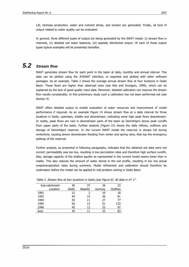
5.4 Spatially distributed results One of the strongest point of SWAT, and the HRU plotting software developed by FutureWater, is that

all terms of the water balance can be evaluated at high spatial resolution. A typical example is shown

in Figure 19, presenting the spatial distribution in actual evapotranspiration. The Figure indicates that

the ET of the natural vegetation is relatively low, which is most likely due to soil characteristics

included in the model that are based on low quality data. Most likely permeability is lower than reality

and storage capacity of the shallow aquifer is probably too small. Due to the low ET runoff to rivers

and streams is very high and soil moisture storage is low. As indicated earlier, storage capacity of

shallow aquifer systems as represented in the current model is probably also too low.

23/30


Water yield, defined as the amount of water contributing to stream flow, is plotted in Figure 20. This

water yield is a composite of the following processes:

WYLD = SURQ + LATQ + GWQ – TLOSS

where WYLD is total water yield, SURQ is surface runoff, LATQ is lateral runoff, GWQ is groundwater

runoff, and TLOSS is seepage losses in channels.

Interesting is that the irrigated areas (see Figure 7) dominantly contribute to the stream flow in Gediz

river.

Based on data used to build the model, groundwater runoff is the dominant factor to water yield (see

Figure 21 and Figure 22; note the different scale). Especially in the irrigated areas, groundwater runoff

contributing to stream flow is high. In the current model setup, groundwater irrigation was only

assumed for areas upstream, resulting in unrealistically high groundwater tables in the downstream

irrigation areas. SWAT offers the opportunity to include this groundwater irrigation, which will result in

a more realistic representation of reality.

Figure 19. Actual evapotranspiration (ET) in 1993.

Figure 20. Water yield contributing to stream flow in 1993.

Actual ET(mm/y)

201202 - 300301 - 400401 - 500501 - 750751 - 10001001 - 12501251 - 1500

Gediz SWATWatManSup

0 25 5012.5 km

Water yield(mm/y)

0 - 100101 - 200201 - 232233 - 300301 - 400401 - 500501 - 700

Gediz SWATWatManSup

0 25 5012.5 km

24/30


Figure 21. Surface runoff in 1993.

Figure 22. Groundwater runoff in 1993.

Surface runoff(mm/y)

01 - 56 - 1011 - 2526 - 5051 - 7576 - 100

Gediz SWATWatManSup

0 25 5012.5 km

GW runoff(mm/y)

0 - 5051 - 100101 - 150151 - 200201 - 250251 - 300301 - 400401 - 500501 - 750

Gediz SWATWatManSup

0 25 5012.5 km

25/30


26/30


6 Conclusions Water managers and decision makers are in need to have better tools and methods to support them.

The project WatManSup was set up to demonstrate what options different tools, separately and

combined, might offer. This report describes one of the components, the physical based one, for the

demonstration case in Turkey. The tool used, SWAT, can be considered as state-of-the-art and has

been used numerous times in other cases. SWAT has been developed further, refined and expanded

by FutureWater during several modelling studies.

As indicated earlier, the model developed for Gediz Basin has not been fully calibrated and validated,

and results should therefore only be considered as demonstration of the options SWAT offers to

evaluate output. Examples on further model refinement and calibration can be found elsewhere (e.g.

Kauffman and Droogers, 2007; Immerzeel and Droogers, 2007)

In summary the following conclusions can be drawn from the demonstration case in Gediz Basin:

• The strength of the physical component SWAT in Integrated Water Management Support

Methodologies is that all physical processes are included in the model. All aspects of the

hydrological cycle can be evaluated, including crop growth, irrigation, and water quality.

• The completeness of the tool makes it highly data demanding and somewhat complex. At the

same time sufficient new technologies are developed and under development to overcome

these data shortage problems. Remote sensing techniques, public domain data sources and

improved calibration approaches are typical examples that can be applied nowadays.

• Results presented for the demonstration case of Gediz Basin reveal that more emphasis

should be given to verification and calibration of the model. It is clear that characteristics of

soils, especially storage capacity and permeability, are keys to improve the model. Data might

be collected on these parameters, but at the same time calibration on stream flows and/or

ET, estimated by remote sensing, can be used to update the model.

• The physical tool SWAT should only be used to support water managers and decision makers

if their questions are related to physical processes. If problems are related to strategic

planning of water allocation, the WEAP approach is preferred (see Van Loon et al., 2007).

Typical examples of questions to be answered using SWAT are: impact and adaptation to

climate change, improved evapotranspiration management including deficit irrigation, changes

in land cover and/or crops, and contribution of rainfall to water resources.

27/30


28/30


References

Droogers, P., G.W. Kite, and W. Bastiaanssen. 1999. Land cover classification using public domain

datasets: example for Gediz Basin, Turkey. In Proceedings of International Symposium on

Arid Region Soils. Menemen, Turkey, 21-25 September 1998. p 34-40

DSI. 2006. Devlet Su İşleri, http://www.dsi.gov.tr/, visited on 06/04/2007

FAO. 2000. Digital soil map of the world and derived soil properties on cd-rom. Food and Agricultural

Organization. Rome. http://www.fao.org/AG/agl/agll/dsmw.htm

FutureWater. 2007. FutureWater, Science for Solutions. http://www.futurewater.nl

Immerzeel, W., P. Droogers. 2006. Spatial calibration of a distributed hydrological model using Remote

Sensing derived evapotranspiration in the Upper Bhima catchment, India. Hydrological

Processes (under review).

Kauffman, S., P. Droogers. 2007. Green and Blue Water Services Tana River Basin, Kenya. Assessment

of improved soil and water management scenarios using an integrated modelling framework.

ISRIC World Soil Information Report no 2007-03.

Kite, G.W. and P. Droogers. 1999. Irrigation modelling in a basin context. Water Resources

Development 15: 43-54.

Monteith, J.L. 1977. Climate and the efficiency of crop production in Britain. Phii. Trans. Res. Soc.

London Ser. B. 281 :277-329.

Neitsch, S.L., J.G. Arnold, J.R. Kiniry, J.R. Williams, K.W. King. 2002a. Soil and Water Assessment Tool,

Theoretical Documentation. Texas Water Resources Institute, College Station, Texas, TWRI

Report TR-191.

Neitsch, S.L., J.G. Arnold, J.R. Kiniry, R. Srinivasan, J.R. Williams. 2002b. Soil and Water Assessment

Tool, User’s Manual. Texas Water Resources Institute, College Station, Texas, TWRI Report

TR-192.

SMART. 2007. SMART: Sustainable Management of Scarce Resources in the Coastal Zone.

http://www.ess.co.at/SMART/CASES/TR/turkey.html

SWAT. 2007. http://www.brc.tamus.edu/swat/

THAEM. 1999. Irrigation in the basin context (in Turkish). http://www.thaem.gov.tr/gedizprj.htm

Van Loon, A., H. Mathijssen, P. Droogers. 2007. Water Evaluation and Planning System, Gediz Basin –

Turkey. WatManSup Report No. 5. http://www.futurewater.nl/watmansup/

Van Loon, A., P. Droogers. 2007. Soil and Water Assessment Tool, Kitui – Kenya. WatManSup Report

No. 3. http://www.futurewater.nl/watmansup/

USGS. 2006. HYDRO1K, U.S. Geological Survey. http://edc.usgs.gov/products/elevation/gtopo30/

hydro/readme.html#References

WatManSup. 2007. Integrated Water Management Support Methodologies for Turkey and Kenya.

http://www.futurewater.nl/watmansup/

Williams, J.R., C.A. Jones, P.T. Dyke. 1984. A modeling approach to determining the relationship

between erosion and soil productivity. Trans. ASAE 27:129-144.

29/30


30/30

Documents

Soil and Water Assessment Tool, Gediz â€“ Turkey - FutureWater