UNIVERSIDADE FEDERAL DO RIO GRANDE DO SULINSTITUTO DE INFORMÁTICA

CURSO DE ENGENHARIA DE COMPUTAÇÃO

GENNARO SEVERINO RODRIGUES

Software Errors Analysis at the Zynq SoCARM Embedded Processor

Work presented in partial fulfillmentof the requirements for the degree ofBachelor in Computer Engeneering

Advisor: Prof. Dr. Fernanda Lima Gusmão

Porto AlegreDezembro 2015

UNIVERSIDADE FEDERAL DO RIO GRANDE DO SULReitor: Prof. Carlos Alexandre NettoVice-Reitor: Prof. Rui Vicente OppermannPró-Reitor de Pós-Graduação: Prof. Vladimir Pinheiro do NascimentoDiretor do Instituto de Informática: Prof. Luis da Cunha LambCoordenador do Curso de Engenharia de Computação: Prof. Marcelo GötzBibliotecária-chefe do Instituto de Informática: Beatriz Regina Bastos Haro

“Or has the potter no right over the clay,

to make from the same lump

one piece of pottery for honor

and another for dishonor?”

— THE BIBLE, ROMANS 9:21

ACKNOWLEDGMENTS

During my years of study and academical development many people were fundamental

to my progress. One can not achieve great things alone, and a student in special would never

be able to abandon the darkness of nescience without the support of his peers. For that reason,

I thank all professors and teachers that had any influence on my life whatsoever, for every

experience is a chance for growing.

Those who have stood by my side during my graduation are also deserving of recogni-

tion. Many of the great things I’ve accomplished in my professional life would not be possible

without the moral and technical support of colleagues like Marcelo Brandalero, Jeckson Souza,

Alessandra Leonhardt, João Leidens and Rafael Finkelstein. There were uncountable others,

most of which equally supportive, but would make this list too long to be literally acceptable.

I also thank my friends from Polytech Montpellier, who gave me support when I needed

the most during my studies abroad, and showed me a different view of the world and approach

for engineering. I believe that having multiple views of the engineering application is primordial

for ultimate usability of this tool. Therefore, I feel obliged to thank all the engineers who,

during my internship at AEL Systems S/A, taught me some of the most valuable lessons of my

professional life.

My final thanks go to Prof. Fernanda Lima Kastensmidt, who provided me academical

guidance during my last years as a researcher at my graduation, and immeasurable support in

this work’s effort.

ABSTRACT

This work presents an analysis of the occurrence of software errors at the Xilinx Zynq-7000

programmable SoC, which adopts two ARM processing cores (more specifically a Cortex-A9

MPx2). The goal is to analyze the software errors occurrence due to failures at dual-core em-

bedded processors. A comparison of the errors occurrence at different applications for different

uses was developed, as well as comparative analysis of the applications behaviors for both it’s

parallel and serial versions. To achieve those, a fault injection tool was developed - using the

OVP simulator - which is capable of injection faults at application runtime. The analysis method

consists into comparing fault-injected executions with a fault-free application execution. The

error types, count, and effects on the final results were extracted from the developed tool, and

were used to develop analyses on how to engage, treat, and prevent the generated errors. Both

the parallel and sequential versions of the applications were executed on the very same simu-

lated environment (a version of embedded Linux) and the parallel versions were implemented

using pthreads.

Keywords: Failure Injection. Error Analysis. ARM. Dual-core. Simulation.

Análise de Erros em Software no Processador ARM Embarcado no SoC Zynq

RESUMO

Este trabalho apresenta uma análise da ocorrência de erros em software no SoC Zynq-7000,

comercializado pela Xilinx, que possui dois núcleos de processamento ARM embarcados (mais

especificamente o Cortex-A9 MPx2). O objetivo é analisar a ocorrência de erros devido ao

aparecimento de falhas em software em processadores embarcados dual-core. Foi feita uma

comparação da ocorrência de erros em aplicações de propósitos variados, assim como análises

comparativas do comportamento de cada aplicação quando em sua versão serial e paralela.

Para tanto, desenvolveu-se uma ferramenta para a inserção de falhas, utilizando o simulador

OVP, que é capaz de inserir falhas durante a execução de uma aplicação. O método de análise

consiste em comparar execuções da aplicação onde falhas foram injetadas com uma execução

livre de falhas. Assim foi possível analisar quais tipos de erros foram gerados pelas falhas,

sua quantidade, efeitos no resultado final da execução e desenvolver análises para abordagens

futuras de como evitá-los ou tratá-los. As versões paralelas das aplicações são implementadas

usando pthreads e ambas as versões paralelas e sequenciais foram executadas em uma versão

de Linux embarcado.

Palavras-chave: Injeção de Falhas. Análise de Erros. ARM. Dual-core. Simulação.

LIST OF ABBREVIATIONS AND ACRONYMS

SoC System on a Chip

FPGA Field-Programmable Gate Array

COTS Commercial-Off-The-Shelf

RCTA Radio Technical Commission for Aeronautics

OS Operation System

OVPSim OVP Simulator

FIM Fault Injector Module

SDC Silent Data Corruption

DMA Direct Memory Access

SEE Single Event Effect

SEU Single Event Upset

SBU Single Bit Upset

MBU Multibit Upset

SEFI Single Event Interrupt

SEL Single Event Latch-up

AVF Architectural Vulnerability Factor

SER Soft Error Rate

FIT Failure In Time

ICOUNT Instruction Counter

FI Fault Injection

LIST OF FIGURES

Figure 2.1 Zync-7000 SoC diagram......................................................................................... 14

Figure 3.1 Fault Injection Environment Model........................................................................ 22

Figure 4.1 FIM Injection Organization .................................................................................... 26Figure 4.2 Injection Phases ...................................................................................................... 27Figure 4.3 Simulation Infrastructure ........................................................................................ 29

Figure 5.1 Simulation CPU Information.................................................................................. 36Figure 5.2 Dijkstra Sequential Version Results ....................................................................... 37Figure 5.3 Dijkstra Parallel, One Queue Version Results ........................................................ 38Figure 5.4 Dijkstra Parallel, N Queues Version Results .......................................................... 38Figure 5.5 Susan Sequential Version Results........................................................................... 39Figure 5.6 Susan Parallel Version Results................................................................................ 39Figure 5.7 Stringsearch Sequential Version Results ................................................................ 40Figure 5.8 Stringsearch Parallel Version Results ..................................................................... 40Figure 5.9 SHA-1 Sequential Version Results ......................................................................... 41Figure 5.10 SHA-1 Parallel Version Results............................................................................ 41Figure 5.11 Dijkstra Results Comparison ................................................................................ 42Figure 5.12 Susan Results Comparison ................................................................................... 43Figure 5.13 Stringsearch Results Comparison......................................................................... 44Figure 5.14 SHA-1 Results Comparison.................................................................................. 45

LIST OF TABLES

Table 4.1 Error type classifications. ......................................................................................... 33

Table 5.1 Register Coverage for Fault Injection at Dijkstra..................................................... 46Table 5.2 Register Coverage for Fault Injection at Susan ........................................................ 47Table 5.3 Register Coverage for Fault Injection at Stringsearch.............................................. 47Table 5.4 Register Coverage for Fault Injection at SHA-1 ...................................................... 48

CONTENTS

1 INTRODUCTION................................................................................................................ 112 MOTIVATION ..................................................................................................................... 132.1 The Problem ..................................................................................................................... 142.2 The Approach................................................................................................................... 153 RELATED WORK .............................................................................................................. 163.1 Radiation Impact on Electronics .................................................................................... 163.2 Types of Failures .............................................................................................................. 173.3 Architectural Vulnerability Factor................................................................................. 173.4 Operation System Influence on the Cross-Section........................................................ 183.5 Soft Error Rate................................................................................................................. 193.6 Fault Injection Methods .................................................................................................. 193.6.1 Physical Fault Injection................................................................................................... 203.6.2 Logical Fault Injection.................................................................................................... 203.6.3 Emulation-based Fault Injection ..................................................................................... 213.6.4 Simulation-based Fault Injection .................................................................................... 214 METHODOLOGY .............................................................................................................. 234.1 OVP Simulator ................................................................................................................. 234.2 Fault Injection Module (FIM)......................................................................................... 254.2.1 Simulation Injection Phases............................................................................................ 274.2.1.1 Golden Phase ............................................................................................................... 274.2.1.2 Fault Creation Phase .................................................................................................... 284.2.1.3 Execution Phase ........................................................................................................... 284.2.1.4 Error Detection Phase .................................................................................................. 284.2.1.5 Final Phase ................................................................................................................... 294.2.2 Simulation Infrastructure ................................................................................................ 294.3 Benchmarks ...................................................................................................................... 304.3.1 Susan ............................................................................................................................... 304.3.2 Dijkstra............................................................................................................................ 314.3.3 Stringsearch..................................................................................................................... 314.3.4 SHA-1 ............................................................................................................................. 314.4 Simulation Outputs.......................................................................................................... 324.4.1 Errors............................................................................................................................... 324.4.2 Expected Results............................................................................................................. 335 RESULTS.............................................................................................................................. 355.1 Experimental Setups........................................................................................................ 355.2 Testing Environment........................................................................................................ 355.3 Results ............................................................................................................................... 365.3.1 Dijkstra Simulation Results ............................................................................................ 375.3.2 Susan Simulation Results................................................................................................ 385.3.3 Stringsearch Simulation Results ..................................................................................... 395.3.4 SHA-1 Simulation Results.............................................................................................. 405.4 Failures Analysis .............................................................................................................. 415.5 Register Coverage Analysis............................................................................................. 466 CONCLUSION .................................................................................................................... 50REFERENCES........................................................................................................................ 52

11

1 INTRODUCTION

As the dimensions and operating voltages of computer electronics are reduced to sat-

isfy the consumer’s insatiable demand for higher density, functionality, and lower power, their

sensitivity to radiation increases dramatically. At (DODD; MASSENGILL, 2003) it’s shown

that there are a plethora of radiation effects in semiconductor devices that vary from data dis-

ruptions to permanent damage, ranging from parametric shifts to complete device failure. The

“soft” single event effects (SEEs) are of primary concern for commercial applications. Op-

posed to those, are the “hard” SEEs and dose-rate related radiation effects, that are predominant

in space and military environments. As the name implies, SEEs are device failures induced by

a single radiation event.

The history of radiation effects on technology begins early, as shown by (CODERRE et

al., 2006). It was noted by investigators that electroscopes could remain slightly ionized after

their use. Later it was found that this effect could be reduced with lead blocks protections,

which implied an external radiation source as the cause of the problem. This type of radiation

was also seen at the top of the Eiffel tower - which was too high for being radium effects - which

led to the theory that the source was in the atmosphere. Balloon experiments would later show

that the radiation intensity increased with altitude.

The first applications to have some interest on SEEs were specific: aero-space, high-

reliability, nuclear facilities equipment, implantable medical devices. Today, however, the in-

creasing complexity and integration level of modern systems makes them sensitive to the same

effects. It is expected from the new technologies to perform safely and reliably. There is a

big number of solutions for error handling: from special radiation-hardened circuit designs,

as developed by (CALIN; NICOLAIDIS; VELAZCO, 1996), to localized error detection and

correction (as detailed at (ANDO et al., 2003)) and architectural redundancy, as shown by

(MUKHERJEE; KONTZ; REINHARDT, 2002) and (WOOD, 1999). However, all of these

approaches introduce a significant penalty in performance, power, die size, and design time.

Because of that, designers must carefully weigh the benefits of adding these techniques against

their cost. While a microprocessor with inadequate protection from transient faults may prove

useless due to its unreliability, excessive protection may make the resulting product noncom-

petitive in cost and performance. Unfortunately, tools and techniques to estimate processor

transient error (i.e., a non-permanent error) rates are not fully available nor understood. Also,

because a comprehensive error-handling strategy is best designed in from the ground up, these

estimates are needed early in the design cycle.

12

To successfully achieve the optimal balance between fault-tolerance and its costs, it is of

uttermost importance to develop a trustworthy method for the system failure behavior analysis.

The generally applied method is to inject faults in the system to be tested, which can be done in

a variety of ways (as will be defined at Section 3.6).

This work provides an analysis of the failures behavior on software at the Zynq SoC,

which combines the dual-core ARM Cortex-A9 processor with an FPGA fabric. The SoC is

simulated using the OVP simulator, and failures are generated and injected in the benchmark

applications using a fault injector framework developed to be fast and flexible, which is called

OVPSim-FIM. Each benchmark ran on top of Linux and had both a parallel and a sequential

version of the algorithm tested. The parallel versions of the algorithms were programmed using

POSIX threads. The results of the sequential and parallel algorithm versions of each benchmark

are compared, in the light of the errors generated by the injected faults. Each batch of tests have

the same number of faults randomly injected in random registers of the embedded ARM Cortex-

A9 processor. The goal of this work is to analyze software errors, so the simulator will simulate

the Zynq SoC ARM processor only (not the FPGA fabric).

The simulation results showed a tendency on almost every case for the parallel version

of an algorithm to be more sensitive to silent data corruption failures than the sequential algo-

rithm. Nevertheless, each one of the different benchmarks used for testing presented a different

behavior, and even an unique difference between the sequential execution simulation results and

the parallel ones. This supports the idea that the overall dependability of a system has a strong

relation with the implementation strategy of the application that is running in the system. A

similar idea was also supported by (MUKHERJEE et al., 2003).

The work has the following organization structure: Section 2 presents a continuation

to the introduction, presenting the motivations behind the choice of the used method and sys-

tem being evaluated. Section 3 presents the state-of-the-art concepts and related work on the

field. Section 4 presents the simulation details, the model used, fail injection and simulator ar-

chitecture, and simulation-related information. The results of the simulation are presented and

discussed at Section 5. Section 6 presents the conclusion and future work ideas.

13

2 MOTIVATION

Safety-critical projects today make predominately use of single-core processor archi-

tectures. There are reasons to limit safety-critical applications for single-core architectures

(alongside with others hardware limitations). Performance is not the main concern for that area

of engineering. DO-254 certification, for instance, which is a certification for hardware design

needed for avionics systems to operate in most of the world, is hardly attainable for multi-core

systems due to its memory and processor unit design limitations. The works of (HILDERMAN;

BAGHI, 2007) trace a good view of the usually desired certifications and how to obtain them.

Nevertheless, the tendency for processors unit industry is to turn to multi-core to achieve better

performance.

Such a demand for higher performance processors tends to impact the processor units’

types and resources available for markets with smaller demand (such as aerospace and others

critical applications), which have conflicting technological interests. The developers, manufac-

turers, and vendors tend to focus on the satisfaction of their larger market shares. As safety-

critical systems are not the most abundant consumers of the industry, they may have to adapt

to make use of what the industry has to offer, which is hardware designed with a focus on per-

formance, not on fault-tolerance. It’s unsafe to believe even that single-core architectures will

keep being developed for long, let alone that they may keep an evolving pace.

In a matter of fact, the safety-critical applications industry has turn to COTS (Commercial-

Off-The-Shelf) systems as a valid alternative to specific hardware for safety-critical applica-

tions, for radiation-hardened hardware are expensive. Hardened devices bound to hardware

limitations, such as those defined by the DO-254 certification document. COTS systems, on

the other hand, are typically low cost, much more flexible and have a low power consumption.

Those systems have been used in safety-critical applications like biomedical devices, aircraft

and satellites control circuitry and automotive systems. The Zynq™-7000 All Programmable

SoC, for instance, is capable of serving a wide range of safety-critical applications, such as

avionics communications and missile and smart ammunition control systems. As shown at Fig-

ure 2.1, the Zynq SoC possess both a programmable logic and ARM cores, which is one of the

main reasons why it has been showing off a great potential for those applications.

14

Figure 2.1 – Zync-7000 SoC diagram

Source: Xilinx Inc.

2.1 The Problem

A problem here arises on safety: radiation-induced failure rate is not negligible on

nowadays’ electronic systems, neither for safety-critical applications nor ordinary consumer

proposes. Safety-critical applications, such as spacecraft boarded computing and aeronautical

navigation systems, are much more vulnerable to radiation than the regular use of computation.

Therefore the acknowledgment of how the overall system will react to faults is important, in

special for safety-critical applications. Because of the industry tendency to adopt multi-core

processors it’s also relevant to study the behavior of parallel applications applied on COTS

systems with embedded multi-core processors.

Safety-critical operations also need to manage the execution of many applications shar-

ing resources. Especially for avionics applications, software design needs to be certified by the

Radio Technical Commission for Aeronautics (RTCA) to operate, just like the hardware design.

For software, it is desired the DO-178B/C certificate. This certificate’s exigencies are highly

conflicting with memory sharing software systems, imposing a large number of limitations and

safety measures to avoid failures and catastrophic errors. To guarantee a safe management of

15

those resources, the use of a general purpose OS is attractive, once developing a specific OS

for a radiation-hardened system would be costly. Also, running bare-metal applications on a

system would be a waste of resources.

2.2 The Approach

An OS is fundamental to provide a good user interface and experience. That makes the

use of a general purpose OS - like embedded Linux - a good alternative. This is one of the

reasons why, at this work, the tests will run under Linux. Given that the idea is to analyze the

reaction of adopted applications for industrial use (applied to embedded systems, of course),

using an embedded version of Linux is a good choice.

As mentioned at Section 1, this work provides an analysis of the failures behavior on

software at the Zynq SoC and compares the parallel (which makes use of POSIX threads) and

sequential versions of algorithms results after fault injection. With this data collected, it should

be possible to deeply study what are the differences between running a sequential or a parallel

algorithm under strong radiation (or any other hostile environment), and how it affects the types

of generated errors and faults. The work also provides a study of fault injections results on one

of the most used COTS hardware in the industry, especially for safety-critical projects (i.e., the

Zynq SoC). The faults are injected on software running on Linux, and the area affected by the

fault injections is the ARM cores only.

16

3 RELATED WORK

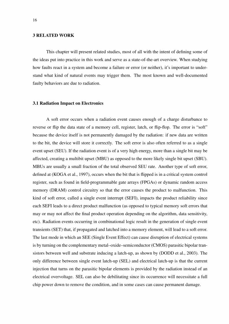
This chapter will present related studies, most of all with the intent of defining some of

the ideas put into practice in this work and serve as a state-of-the-art overview. When studying

how faults react in a system and become a failure or error (or neither), it’s important to under-

stand what kind of natural events may trigger them. The most known and well-documented

faulty behaviors are due to radiation.

3.1 Radiation Impact on Electronics

A soft error occurs when a radiation event causes enough of a charge disturbance to

reverse or flip the data state of a memory cell, register, latch, or flip-flop. The error is “soft”

because the device itself is not permanently damaged by the radiation: if new data are written

to the bit, the device will store it correctly. The soft error is also often referred to as a single

event upset (SEU). If the radiation event is of a very high energy, more than a single bit may be

affected, creating a multibit upset (MBU) as opposed to the more likely single bit upset (SBU).

MBUs are usually a small fraction of the total observed SEU rate. Another type of soft error,

defined at (KOGA et al., 1997), occurs when the bit that is flipped is in a critical system control

register, such as found in field-programmable gate arrays (FPGAs) or dynamic random access

memory (DRAM) control circuitry so that the error causes the product to malfunction. This

kind of soft error, called a single event interrupt (SEFI), impacts the product reliability since

each SEFI leads to a direct product malfunction (as opposed to typical memory soft errors that

may or may not affect the final product operation depending on the algorithm, data sensitivity,

etc). Radiation events occurring in combinational logic result in the generation of single event

transients (SET) that, if propagated and latched into a memory element, will lead to a soft error.

The last mode in which an SEE (Single Event Effect) can cause disruption of electrical systems

is by turning on the complementary metal–oxide–semiconductor (CMOS) parasitic bipolar tran-

sistors between well and substrate inducing a latch-up, as shown by (DODD et al., 2003). The

only difference between single event latch-up (SEL) and electrical latch-up is that the current

injection that turns on the parasitic bipolar elements is provided by the radiation instead of an

electrical overvoltage. SEL can also be debilitating since its occurrence will necessitate a full

chip power down to remove the condition, and in some cases can cause permanent damage.

17

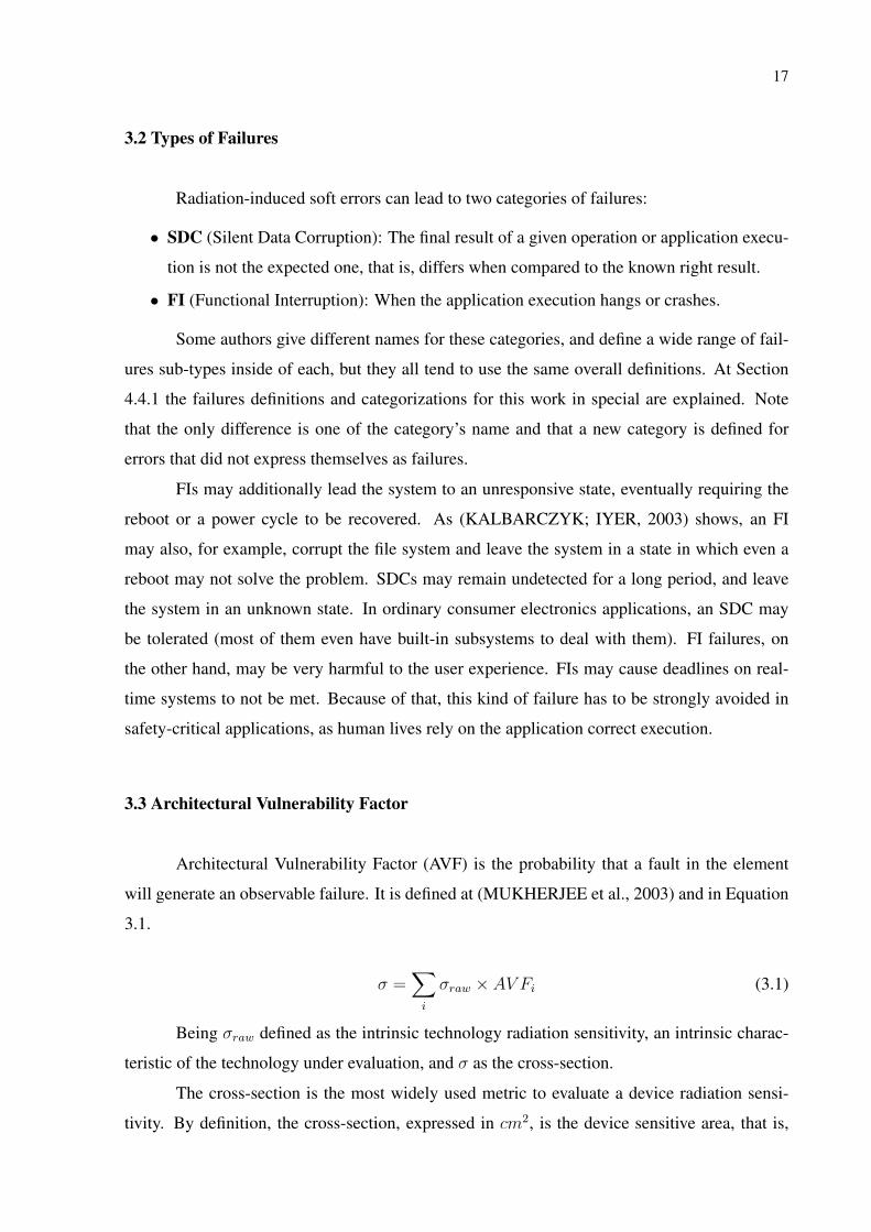
3.2 Types of Failures

Radiation-induced soft errors can lead to two categories of failures:

• SDC (Silent Data Corruption): The final result of a given operation or application execu-

tion is not the expected one, that is, differs when compared to the known right result.

• FI (Functional Interruption): When the application execution hangs or crashes.

Some authors give different names for these categories, and define a wide range of fail-

ures sub-types inside of each, but they all tend to use the same overall definitions. At Section

4.4.1 the failures definitions and categorizations for this work in special are explained. Note

that the only difference is one of the category’s name and that a new category is defined for

errors that did not express themselves as failures.

FIs may additionally lead the system to an unresponsive state, eventually requiring the

reboot or a power cycle to be recovered. As (KALBARCZYK; IYER, 2003) shows, an FI

may also, for example, corrupt the file system and leave the system in a state in which even a

reboot may not solve the problem. SDCs may remain undetected for a long period, and leave

the system in an unknown state. In ordinary consumer electronics applications, an SDC may

be tolerated (most of them even have built-in subsystems to deal with them). FI failures, on

the other hand, may be very harmful to the user experience. FIs may cause deadlines on real-

time systems to not be met. Because of that, this kind of failure has to be strongly avoided in

safety-critical applications, as human lives rely on the application correct execution.

3.3 Architectural Vulnerability Factor

Architectural Vulnerability Factor (AVF) is the probability that a fault in the element

will generate an observable failure. It is defined at (MUKHERJEE et al., 2003) and in Equation

3.1.

σ =∑i

σraw × AV Fi (3.1)

Being σraw defined as the intrinsic technology radiation sensitivity, an intrinsic charac-

teristic of the technology under evaluation, and σ as the cross-section.

The cross-section is the most widely used metric to evaluate a device radiation sensi-

tivity. By definition, the cross-section, expressed in cm2, is the device sensitive area, that is,

18

the area that generates a failure if hit by a particle. Given a specific resource in the system, its

cross-section can be described by a combination of the σraw attenuated by the AVF (as explicit

at Equation 3.1).

Although the AVF can be estimated through fault injection, a deep knowledge of the

device implementation, sometimes even of register-transfer-level description, is required. Those

are the type of information rarely available for COTS systems. The system cross-section can be

obtained experimentally through accelerated radiation test campaigns. The observed number of

errors during the test is divided into the particle fluence, i.e., the number of particles hitting the

device per unit area, yielding a cross-section.

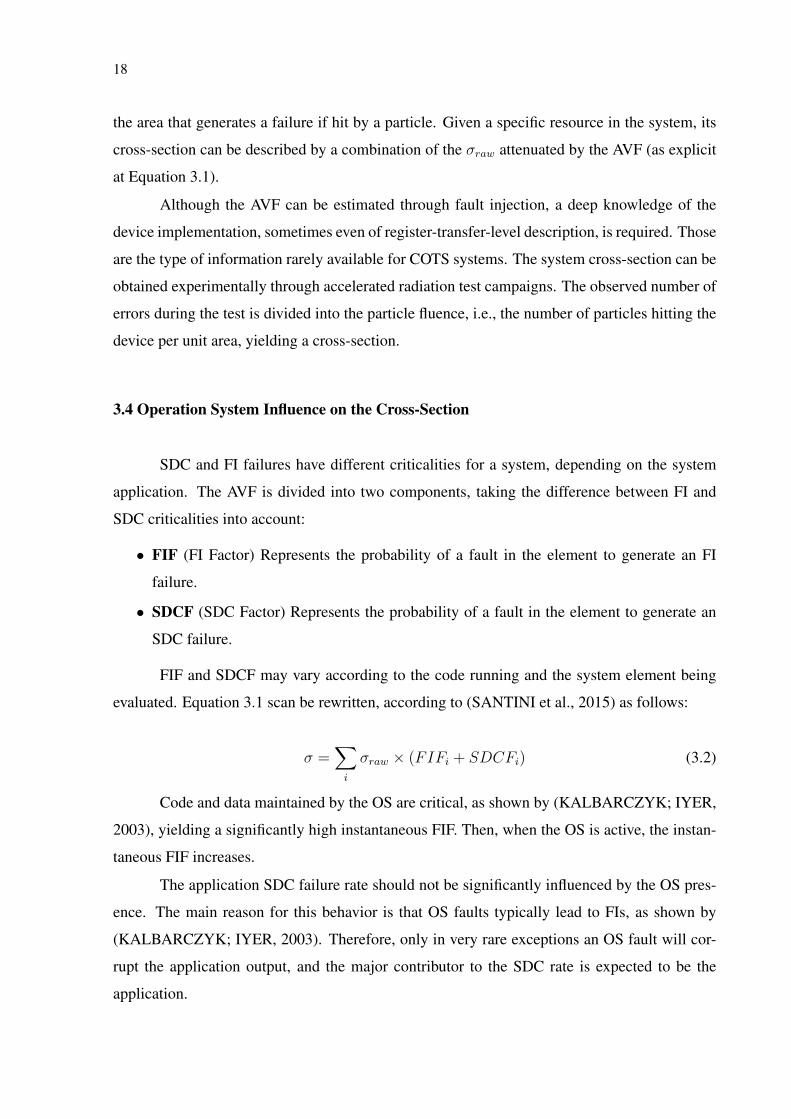
3.4 Operation System Influence on the Cross-Section

SDC and FI failures have different criticalities for a system, depending on the system

application. The AVF is divided into two components, taking the difference between FI and

SDC criticalities into account:

• FIF (FI Factor) Represents the probability of a fault in the element to generate an FI

failure.

• SDCF (SDC Factor) Represents the probability of a fault in the element to generate an

SDC failure.

FIF and SDCF may vary according to the code running and the system element being

evaluated. Equation 3.1 scan be rewritten, according to (SANTINI et al., 2015) as follows:

σ =∑i

σraw × (FIFi + SDCFi) (3.2)

Code and data maintained by the OS are critical, as shown by (KALBARCZYK; IYER,

2003), yielding a significantly high instantaneous FIF. Then, when the OS is active, the instan-

taneous FIF increases.

The application SDC failure rate should not be significantly influenced by the OS pres-

ence. The main reason for this behavior is that OS faults typically lead to FIs, as shown by

(KALBARCZYK; IYER, 2003). Therefore, only in very rare exceptions an OS fault will cor-

rupt the application output, and the major contributor to the SDC rate is expected to be the

application.

19

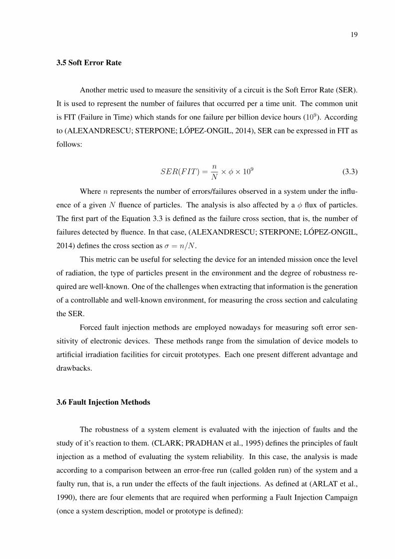
3.5 Soft Error Rate

Another metric used to measure the sensitivity of a circuit is the Soft Error Rate (SER).

It is used to represent the number of failures that occurred per a time unit. The common unit

is FIT (Failure in Time) which stands for one failure per billion device hours (109). According

to (ALEXANDRESCU; STERPONE; LÓPEZ-ONGIL, 2014), SER can be expressed in FIT as

follows:

SER(FIT ) =n

N× φ× 109 (3.3)

Where n represents the number of errors/failures observed in a system under the influ-

ence of a given N fluence of particles. The analysis is also affected by a φ flux of particles.

The first part of the Equation 3.3 is defined as the failure cross section, that is, the number of

failures detected by fluence. In that case, (ALEXANDRESCU; STERPONE; LÓPEZ-ONGIL,

2014) defines the cross section as σ = n/N .

This metric can be useful for selecting the device for an intended mission once the level

of radiation, the type of particles present in the environment and the degree of robustness re-

quired are well-known. One of the challenges when extracting that information is the generation

of a controllable and well-known environment, for measuring the cross section and calculating

the SER.

Forced fault injection methods are employed nowadays for measuring soft error sen-

sitivity of electronic devices. These methods range from the simulation of device models to

artificial irradiation facilities for circuit prototypes. Each one present different advantage and

drawbacks.

3.6 Fault Injection Methods

The robustness of a system element is evaluated with the injection of faults and the

study of it’s reaction to them. (CLARK; PRADHAN et al., 1995) defines the principles of fault

injection as a method of evaluating the system reliability. In this case, the analysis is made

according to a comparison between an error-free run (called golden run) of the system and a

faulty run, that is, a run under the effects of the fault injections. As defined at (ARLAT et al.,

1990), there are four elements that are required when performing a Fault Injection Campaign

(once a system description, model or prototype is defined):

20

• Fault Model: Injected faults are used to model the SEEs at different abstraction levels.

Fault models in the level of the system behavioral model shall be used (for example SBUs

or MBUs). When a COTS is being evaluated, different fault models (adapted to it’s usage

and needs) can be applied.

• Workload: Used to emulate the typical operation of the system under test.

• Observation Elements: Those are applied in the system to classify the effects of the

injected faults. Once a failure is identified, it may be classified as any of the many types

of failures definable. It’s also common to classify the fault itself.

• Measurements: States the degree of dependability of the evaluated system and can be

connected with the metric employed (commonly the SER).

The level of abstraction of the modeled and injected faults and the system model are

to be seriously taken into consideration. Those levels are highly related to the fault injection

method in use at the test. According to (ALEXANDRESCU; STERPONE; LÓPEZ-ONGIL,

2014) there are four different types of fault injection methods, described in the subsequently.

3.6.1 Physical Fault Injection

Physical fault injection consists of using external perturbations sources (e.g. laser beams,

pin forcing) with the intent of provoking electrical disturbances that cause SEEs and conse-

quently soft errors. These tests are done on the final version of a system. This method of test

is the standardized qualification process adopted by space agencies for devices used in their

missions and is also used for other industrial applications and systems developments (such as

avionics, automotive and defense). In those cases, the tests are done exposing the device to a

particle beam (proton, neutron, heavy ions) and calculating the cross section and SER taking

into account the flux and fluence data of the generated beam, alongside with the detected errors.

As (FOUILLAT et al., 2004) shows, laser beams testing provokes similar effects as irradiation

testing, but with some advantages: fault location is more accurate, and campaign cost is lower.

3.6.2 Logical Fault Injection

Logical fault injection consists of injecting the effects of SEUs (modeled at the logical

level) directly at internal elements, making use of specific logic resources (which are built in

the device for debugging purposes, tests, or even interruption management).

21

Software implemented fault injection methods focus on microprocessors, and fault mod-

els are injected during the workload execution phase. SEU effects are generally modeled as a

bit-flip.

This method has a reduced campaign cost, but lesser accuracy (especially when com-

pared with physical fault injection).

3.6.3 Emulation-based Fault Injection

Makes use of programmable devices (such as FPGAs) for circuit emulation. A de-

sign model is available for running fault injection campaigns. Fault injection through device

reconfiguration, modifying the contents of memory elements (bit-flip model) produced some

interesting tools as shown at (ALDERIGHI et al., 2007). Prototyping a modified circuit with

self-injection capability, such as done at (EJLALI; MIREMADI, 2008) allows fast execution of

large fault injection campaigns. Accuracy is dependable of the SEUs models used.

Emulation-based fault injection test campaigns cost much less than physical fault in-

jection ones, and with a good execution time. Reconfiguration solutions have the tendency of

being slower, as fault injection is externally managed.

3.6.4 Simulation-based Fault Injection

Once a good design model is available, simulation-based fault injection may be a good

option, generating very accurate results. The fault injection accuracy depends on the abstraction

level performed by the simulation. There is a big number of cheap tools available that use this

method. Representativeness is moderate, on the other hand, as fault list sampling shall be

done (due to very long simulation times). In some cases, tests can be accelerated by hardware

emulation.

At (HSUEH; TSAI; IYER, 1997), the principles for fault injection environment are de-

fined. Figure 3.1 gives the example of a well-formulated fault injection environment. For a

simulation-based fault injection to be considered reliable, it is necessary to assume that errors

or failures occur according to a determined distribution.

Simulation-based fault injection often makes use of software fault injection (as it is

the case of this work, which will be stated in Section 4). If the target of fault injection is

an application, the fault injector must be somewhere between the application and an OS (if

22

there is one) or directly at the application code. If the target is the OS, the fault injector must

be implemented directly into the OS code. This software approach is flexible, but has some

limitations: it is impossible to inject faults out of the application’s accessible locations, it may

affect the workload and even the structure of the application, and it may fail to capture certain

errors behaviors due to poor time resolution.

Figure 3.1 – Fault Injection Environment Model

(HSUEH; TSAI; IYER, 1997)

23

4 METHODOLOGY

For the tests execution, the OVPSim was used as simulator. Section 4.1 presents with

more detail the simulator and why it’s characteristics were important in the course of works.

Section 4.2 presents the Fault Injector Module: how it was implemented, it’s limitations

and capabilities, and it’s architecture.

A suite of benchmarks was chosen to fit the kind of applications that are usually im-

plemented on COTS SoCs like the Zynq system. It’s also important for the benchmarks to be

compatible with the parallelization techniques and algorithms, and that the benchmark was de-

veloped with parallel architectures in mind. For that purpose, the ParMiBench benchmarks is

a good choice. As shows (IQBAL; LIANG; GRAHN, 2010), ParMiBench consists of paral-

lel implementations of seven algorithms from the single-processor benchmark suite MiBench.

The applications are selected from four domains: Automation and Industry Control, Network,

Office, and Security. A detailed view on each of the used applications is available at Section

4.3.

The simulation’s output data structure and expected results are defined at Section 4.4.

4.1 OVP Simulator

OVPsim is a simulator. It works with a Just-In-Time Code Morphing engine, which

translates target instructions to x86 host instructions dynamically, that is, a binary translation.

It was selected as the simulator used in this work for manly three reasons:

• Speed: OVPSim relies on a JIT-based engine, which enables the simulation of embedded

systems running real application code at the speed of hundreds of MIPS. This provides

faster simulations.

• Development: It is open-source and has an active development and support community,

including processor providers like ARM and MIPS Technologies. The fact that ARM

Ltd. itself provides OVPSim with user support and testing modules makes it a reliable

source of results.

• Tools: OVPSim also provides a library of components with a large number of processor

architectures (e.g. ISAs, like MIPS, ARM, PowerPC) available, as well as peripherals

among available virtual platform simulators. That was a decisive fact: developing the

simulation platform for the ARM processor architecture embedded at the Zynq SoC from

24

scratch would be highly time-consuming, and the existent library provided by OVPSim

is very stable and trustworthy.

Within OVP, models are created by writing code calling functions in a specific modeling

API. These APIs are based around C language, and in this works’ case were used in this same

programming language. Once ARM itself is one of the content providers for OVPSim, it is safe

to believe the model available for the ARM cores at the Zynq SoC are trustworthy. That justifies

the use of the simulator.

To model an embedded system there are several main items to be considered: plat-

forms, processors, peripherals and environment. The platform purely connects and configures

the behavioral components. The processors fetch and execute object code instructions from

the memories, and the peripherals model the components and environment that the operating

system and application software interacts with.

OVP modeling comprises several APIs, but, in this case, one was mostly used: ICM.

ICM is an API used to create the testing platform netlist of the system for use with OVPsim.

ICM allows the instantiation of multiple processors, busses, memories and peripherals. Us-

ing busses, memories and processors can be interconnected in arbitrary topologies. It enables

arbitrary multiprocessor shared memory configurations, and heterogeneous multiprocessor plat-

forms. There are also ICM calls to load application programs into simulated memories and to

simulate the platform. Those last calls were the ones used the most when developing the FIM

(Section 4.2).

On the other hand, OVPSim has obvious limitations. Because of the way it works, some

metrics are hard to measure. The program execution time, for instance, will not be the same of

the real application running in the real device. The OVPSim is cycle accurate and instruction ac-

curate. The only manner to count the passage of "time" is via instructions counters (ICOUNT).

As will be related at Section 4.2 and further, this ICOUNT is the auxiliary value used to define

where to inject a fault and as a breakpoint and pseudo-time measurement. OVPSim does not

simulate the physical environment where the device is at, that is, it’s a plain "software simula-

tor". As it will be further detailed, for this work, only the processor registers are accessed as a

manner to inject faults.

25

4.2 Fault Injection Module (FIM)

As stated before, at Section 3.6, there are different ways of injecting faults in a model to

be tested. This work makes use of simulation-based fault injection (Section 3.6.4).

The Fault Injection Module used in this work was introduced by (ROSA et al., 2015),

and developed under the auspices of the micro electronics post graduation program of UFRGS

(Federal University of Rio Grande do Sul). Just like OVPSim, it works like a set of instructions

and an API, giving the user the capability to inject faults in an application (during runtime in

this case). FIM original code has been modified to fit the needs of this research. The original

FIM code was developed to inject faults on single core processors, so it needed to be rethought

for a wider range of applications. This implies changes from the fault injection module code

itself to the results parser. The overall fault injection architecture, nevertheless, remains the

same.

The FIM has a fault model library (FML) and is capable of using a number of fault

injection techniques (FIT). The user shall be able to use the combination of both FML and FITs

to study the dependability of a given platform, which has three main components: memory,

processor and connections. In this work, the faults are injected in the processor only, more

specifically into registers. A fault injection (FI) model is designed as a bit flip, and contains

a bit to be flipped and the time it will be injected. FIM’s default FI configuration mechanism

relies on a random uniform function. According to (FENG et al., 2010), this is an accepted

fault injection technique, since it covers the majority of faults that occur at low computation

costs applications. During an application execution, this model is loaded and the defined FI is

executed when set to. The fault injection module has a fault monitor function, which checks

the system behavior for failures in the presence of faults, alongside with a failure detection

function which verifies the platform components context at the end of the simulation. With the

data collected from the failure detection function, FIM is capable of detecting and categorizing

those detected failures. Those mechanisms are better defined at Section 4.2.1. Figure 4.1 gives

a glance of the overall OVP simulation and it’s relation with FIM.

FIM is developed with the OVPSim API environment, which possess callback functions.

Callbacks enable the access, modification and control of platform components during the sim-

ulation. Those functions are used to intermediate event exchange between included simulation

modules and OVPSim components. For instance, when predefined events occur (e.g. access

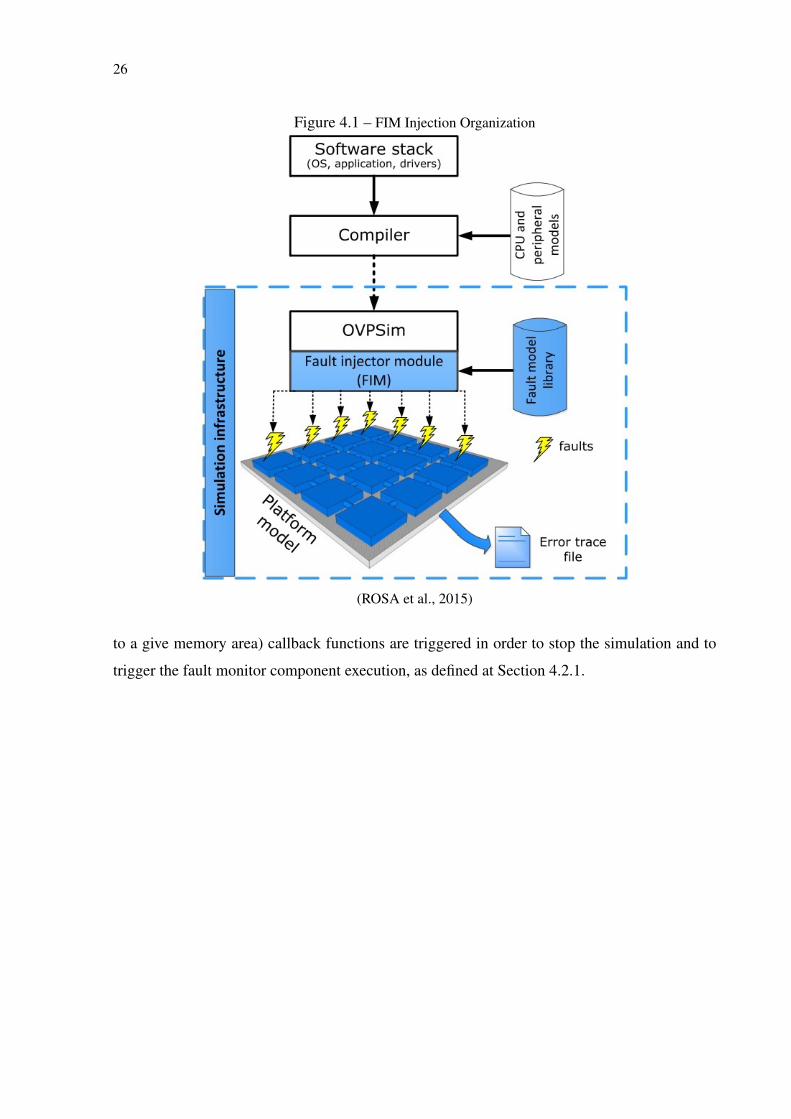
26

Figure 4.1 – FIM Injection Organization

(ROSA et al., 2015)

to a give memory area) callback functions are triggered in order to stop the simulation and to

trigger the fault monitor component execution, as defined at Section 4.2.1.

27

4.2.1 Simulation Injection Phases

The simulation can be divided into five phases according to fault injection activities and

results. Figure 4.2 represents graphically those phases. Next, a more detailed definition for each

phase:

Figure 4.2 – Injection Phases

Author

4.2.1.1 Golden Phase

In this phase, the application is executed at the OVPSim with no fault injections. It’s the

pure execution, to be taken as example of a successful run of the application (the golden run). In

this work’s case, the applications are compiled using the proper cross-compiler, then ran in the

simulator. It’s execution output is then saved in the report we call "golden report". This report

contains vital information, such as the instruction counts (ICOUNT, as defined at Section 4.1)

and the memory map of the application after the successful execution. Those data are registered

during the execution time with the help of the callback functions defined previously.

28

4.2.1.2 Fault Creation Phase

This phase is where faults are configurated and created. The ICOUNT of the Golden

Phase is now used to determine the possible positions of the faults to be generated. As formerly

expressed, one complete instruction is the minimum granularity OVPSim is capable of achiev-

ing, so ICOUNT in this work is being used as a temporal expression. The fault configuration

calculates a random injection time (i.e. ICOUNT) limited between the instruction count when

the application began the execution and when it halts the execution (both counts are registered

during golden phase with the help of callback functions and saved in the golden report) for each

generated fault. The fault location, that is, the register where the fault is to be injected is also

defined randomly. In this work’s context, faults are all single bit flips injected at registers (being

PC a register as well). A bit pattern mask is randomly generated for each fault, to secure a

single bit flip. E.g.: considering a 32-bit architecture, all bits of the mask will be set to 1, except

the one to be flipped, so to set the second bit of a register a mask of value 0xFFFFFFFD shall

be generated. Just like the others fault characteristics, the mask is also randomly generated (but

always designed to flip only one bit). Note that there is no OVPSim execution in this phase.

4.2.1.3 Execution Phase

At the execution phase, the fault monitor function monitors the current ICOUNT while

the application is executed at OVPSim and injects the faults when it is supposed to, i.e., at

the fault’s ICOUNT defined at the fault creation phase. At the correct ICOUNT, the targeted

register is accessed, and an exclusive-OR operation (XOR) is executed between his value and

the generated fault mask, and the resulting value from this operation is then inverted. After the

XOR-invert execution, the resultant value (the register value with a bit flipped) is saved back in

the register, and the application execution goes on.

4.2.1.4 Error Detection Phase

This phase can be defined as a comparison between the golden phase execution (golden

execution) and the execution phase (faulty) execution. FIM considers an error when the fault in-

jected changes the application’s control flow behavior or the memory data results. The proposed

errors classifications are defined at Section 3.2.

29

4.2.1.5 Final Phase

At this phase, the results from all fault injections and errors findings are grouped in a

single report. In case there are more faults to be injected, the simulation execution goes back to

the execution phase. If not, the simulations ends.

4.2.2 Simulation Infrastructure

Depending on the error triggered by the fault injection, the application behavior may

be destructive. The error may, for example, force a processor exception which suspends the

simulation. Some fault injections can generate exceptions like read or write at private memory

region, or trigger a hard fault handler. The FIM and OVPSim frameworks are once again very

useful: a module was created to deal with those exceptions, so that a faulty processor may

continue running. Once this work’s goal is not the study of the treatment nor the mitigation of

errors, they are just captured and registered at reports. The simulation infrastructure then keeps

the simulations for all the unfinished processor models, until they are triggered by an event or

halted by its own reasons (like an exit or break instruction).

OVPSim also gives the option for the user to run multiple simulations at the same time,

as pictures at Figure 4.3. In this work, each of the parallel simulation platform executions are

independent, that is, their result will never affect the others.

Figure 4.3 – Simulation Infrastructure

(ROSA et al., 2015)

30

4.3 Benchmarks

ParMiBench is a benchmark that evaluates the performance of multiprocessor-based

embedded systems. MiBench, on which ParMiBench is based, is a group of applications for

benchmarking of uniprocessor-based embedded systems. ParMiBench provides four bench-

marks categories: Automation and Industry Control, Network, Office, and Security. The dif-

ference between the applications in ParMiBench as compared to those in MiBench is that they

run on multiprocessor-based embedded systems, i.e., the ParMiBench applications are paral-

lel versions of the same applications found in MiBench. The parallel implementations of all

applications are run on embedded Linux, which supports Pthreads and C.

Given that this work studies the behavior of embedded ARM cores, it is a good practice

to use benchmarks developed with that applications in mind. A categorized benchmark enables

the users to examine their design more effectively for a particular market segment of embedded

devices, in this case, COTS used for industrial and safety-critical applications.

ParMiBench exercises the target platform mainly from the scalability perspective. It

exercises the CPU and memory performance of a system while keeping the synchronization

and communication overhead low. Further, it does not particularly stress I/O operation.

Below, each one of the benchmark applications used as workload in this work is detailed.

4.3.1 Susan

Susan is an image recognition application, which recognizes corners and edges in Mag-

netic Resonance Images of the brain. It is used for vision-based quality assurance and performs

adjustments for threshold, brightness, spatial control, and image smoothness. Two different ex-

ecutions are available, depending on the desired processing, varying the size of the algorithm

input data.The small input data is the one used in this work and is a black-white image of a

rectangle while the large input is a complex picture. Susan is composed of different functions,

and these functions are all parallelized by using data decomposition. The decomposition is ap-

plied on the outermost for loop, which iterations are decomposed according to the number of

workers.

31

4.3.2 Dijkstra

Dijkstra calculates the single-source and all pairs shortest paths in a graph represented

by an adjacency matrix.

Dijkstra single-source shortest path has been parallelized using two strategies: single

and multiple queue implementations (both being evaluated in this work). In the first one, all

processors share a single queue, whereas, in the second one, each processor maintains a local

queue. In all pairs shortest path problem, parallel Dijkstra uses a data decomposition strategy

in such a way that one processor handles one vertex to get its single-source shortest paths.

In this work, both strategies for Dijkstra single-source parallel version were tested. The

all pairs solutions are much more time-taking, and as defined at Section 4.2 our fault injection

technique is available only for applications without a very high computation cost, according to

(FENG et al., 2010). Because of that, it is not being evaluated in this work.

4.3.3 Stringsearch

The Stringsearch application searches for a specific word in some given phrases by em-

ploying case sensitive or insensitive comparison algorithms. The partitioning strategy divides

the entire pattern collection into some sub-pattern collections related to the number of workers

allocated.

A file containing the search string and a file containing the patterns are read. For load

balancing, the number of patterns to search for is equally divided among the available workers,

i.e., the number of tasks generated is equal to the number of workers. Then, workers are created

as work is allocated. The workers search in parallel for the patterns, and each of them uses

the sequential implementation of the string search algorithm. Each worker stores the results in

memory. In the end, the master displays the found strings.

4.3.4 SHA-1

SHA-1 (Secure Hash Algorithm) is a cryptographic algorithm, which processes a mes-

saged and produces a message digest. SHA is used to generate digital signatures used for the

secure exchange of cryptographic keys.

The parallel version of SHA uses a master-slave strategy, divided into four stages. The

32

first stage is the calculation of the partition size and the generation of tasks. The second stage

consists of the master reading all the inputs files’ data into memory. At the third stage, the

workers are created. Each one of the workers calculates the digest of the files assigned to it, and

then writes the results to the right memory location (previously defined). Finally at the fourth

stage the master waits for the workers to finish the work and writes the outputs into separated

digest files.

4.4 Simulation Outputs

The final report generated at the Final Phase of the simulation (Section 4.2.1.5) shall then

be interpreted. They most important information for this work’s analysis is the number of error

and their classifications. Next, the error types are defined, alongside with their categorization,

which helps to understand better the effect of the faults on the application run.

4.4.1 Errors

The test reports the count for seventeen types of errors, defined below:

• Masked_Fault: The fault was masked (caused no traceable errors).

• Control_Flow_Data_OK: Divergence between executed instructions during test and gold

phase, but memory is correct.

• Control_Flow_Data_ERROR: Divergence between executed instructions during test

and gold phase, and also between memories.

• REG_STATE_Data_OK: Internal state is incorrect, but memory is correct.

• REG_STATE__ERROR: Both internal state and memory incorrect.

• SDC: Silent data corruption error.

• RD_PRIV: Read privilege exception.

• WR_PRIV:Write privilege exception.

• RD_ALIGN: Read align exception.

• WR_ALIGN: Write align exception.

• FE_PRIV: Fetch privilege exception.

• FE_ABORT: Fetch an inconsistent instruction.

• ARITH: Arithmetic exception in an instruction.

33

• Hang: Application presumably in an infinite loop.

• SEG_FAULT: Segmentation fault error.

• ILLEGAL_INST: Illegal instruction error.

• UNINDENTIFIED: Error caught by Linux, which was unable to identify it’s cause and

type.

Nevertheless, for pratical reasons those types of errors are re-classified on three different

groups, based on their behavior and consequences to the application execution: HANG, SDC

and UNACE. Those groups are defined below.

• SDC: Those errors are detected due to a difference in the final memory from the golden

phase execution and the fault-injected test executions.

• HANG: Those are errors that cause the application to be stuck in a certain point. Not

necessarily in a given instruction, but also in an infinite loop.

• UNACE: Any error that had no influence at all at the final memory state, i.e., memory is

just like it was predicted to be by the golden phase execution.

Table 4.1 classifies the previously defined errors into those new classifications.

Table 4.1 – Error type classifications.Error group Error types

HANG Hang, RD_PRIV, WR_PRIV, RD_ALIGN, WR_ALIGN, FE_PRIV,FE_ABORT and ARITH.

SDC SDC, Control_Flow_Data_ERROR and REG_STATE_Data_ERRORUNACE Masked_Fault, Control_Flow_Data_OK and REG_STATE_Data_OK

This classification helps to better identify the type of error and what may have caused

it. Note that not all of the nineteen types of errors are defined at Table 4.1. That is because this

error grouping definition do not take into account the errors that were caught by Linux.

4.4.2 Expected Results

With the error counting information, this work expects to find differences between the

behavior of parallel algorithms running on dual core processors and the sequential versions of

those same algorithms. It’s believed that with the analysis of the errors on each application, and

the analysis of how each algorithm works, it may be possible to deduct a reason for the expected

differences.

34

Given that parallel systems tend to be much more complex as sequential ones, it would

be no surprise if the parallel versions of the algorithms had much less UNACE errors then the

sequential versions.

Notice that some useful measurements defined at Section 3, such as the SER, are un-

reachable with our simulations outputs. That is because they rely on physical notions that OVP-

Sim is not capable of simulating. As stated by (HSUEH; TSAI; IYER, 1997), fault injection

techniques are suitable for studying emulated faults, but not to provide dependability measures,

such as mean time to failure or availability.

35

5 RESULTS

In this section, the results of the simulation and the fault injection, defined at the Section

4 (Methodology), are presented. Section 5.1 gives a basic overview of the system being simu-

lated while Section 5.2 gives a glance of the system information given by the simulation itself.

Finally, at Section 5.3, the execution outputs of the simulations are graphically presented, and

at Section 5.4 the data is more profoundly compared and analyzed.

5.1 Experimental Setups

As previously defined at Sections 1 and 4, all the faults in this work are injected into the

processor’s registers. The ARM processor embedded at the studied SoC (that is, the Zynq SoC)

is a dual-core ARM Cortex-A9. The system is simulated with the OVP-FIM simulator, defined

at Section 4.1. The fault injection technique was previously introduced at Section 4.2. Each

benchmark execution has one random fault injection, as defined at Section 4.2.1.2.

The model used to simulate the ARM Cortex-A9 was the model developed by ARM Ltd

itself to be specially used at OVPSim, called "Cortex-A9MPx2". This model is used by embed-

ded software developers, which use the OVP simulator to test their ongoing developments. As

the model is extensively used, it is expected for it to be reliable and be a tool to get the most

realistic simulations possible with OVPSim.

The Zynq SoC also possess an FPGA fabric. This element, nevertheless, will not be

simulated, as the focus of this work is to evaluate software errors, more specifically running on

an embedded version of Linux. As the fault injections are limited to the ARM cores registers,

the only part of the SoC simulated is the ARM processor itself. Other elements (such as I/O,

controllers and interconnections), like the ones seen around the ARM cores at Figure 2.1, are

not of importance for this work.

5.2 Testing Environment

The system information on where OVPSim runs is not important, once it shall influence

only the simulation execution time, and in no way the simulation results. It also has no influence

at all in the simulation model execution. The benchmarks execution relies only on the defined

target architecture being simulated. The simulator runs Linux, with kernel version 3.7.1 and

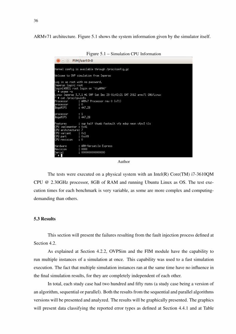
36

ARMv71 architecture. Figure 5.1 shows the system information given by the simulator itself.

Figure 5.1 – Simulation CPU Information

Author

The tests were executed on a physical system with an Intel(R) Core(TM) i7-3610QM

CPU @ 2.30GHz processor, 8GB of RAM and running Ubuntu Linux as OS. The test exe-

cution times for each benchmark is very variable, as some are more complex and computing-

demanding than others.

5.3 Results

This section will present the failures resulting from the fault injection process defined at

Section 4.2.

As explained at Section 4.2.2, OVPSim and the FIM module have the capability to

run multiple instances of a simulation at once. This capability was used to a fast simulation

execution. The fact that multiple simulation instances ran at the same time have no influence in

the final simulation results, for they are completely independent of each other.

In total, each study case had two hundred and fifty runs (a study case being a version of

an algorithm, sequential or parallel). Both the results from the sequential and parallel algorithms

versions will be presented and analyzed. The results will be graphically presented. The graphics

will present data classifying the reported error types as defined at Section 4.4.1 and at Table

37

4.1. The graphics will also express the errors caught by the Linux OS (i.e., SEG_FAULT,

ILLEGAL_INST and UNIDENTIFIED).

5.3.1 Dijkstra Simulation Results

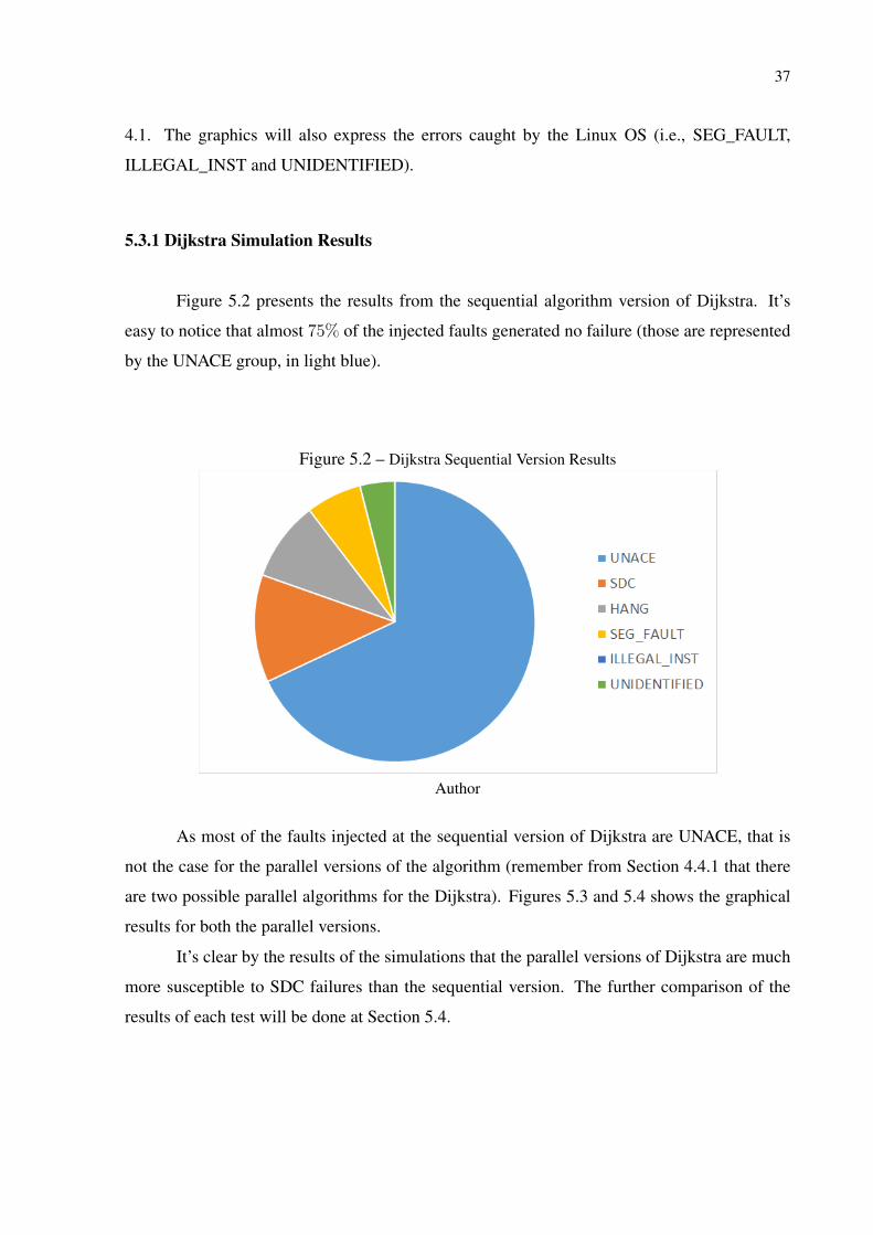
Figure 5.2 presents the results from the sequential algorithm version of Dijkstra. It’s

easy to notice that almost 75% of the injected faults generated no failure (those are represented

by the UNACE group, in light blue).

Figure 5.2 – Dijkstra Sequential Version Results

Author

As most of the faults injected at the sequential version of Dijkstra are UNACE, that is

not the case for the parallel versions of the algorithm (remember from Section 4.4.1 that there

are two possible parallel algorithms for the Dijkstra). Figures 5.3 and 5.4 shows the graphical

results for both the parallel versions.

It’s clear by the results of the simulations that the parallel versions of Dijkstra are much

more susceptible to SDC failures than the sequential version. The further comparison of the

results of each test will be done at Section 5.4.

38

Figure 5.3 – Dijkstra Parallel, One Queue Version Results

Author

Figure 5.4 – Dijkstra Parallel, N Queues Version Results

Author

5.3.2 Susan Simulation Results

The Susan algorithm simulation results are rather different than Dijkstra’s. It’s clear by

its sequential algorithm execution result that this version is more susceptible to SDC failures

than the parallel version. Figures 5.5 and 5.6 shows the results of those simulations. In a

matter of fact, the Susan parallel algorithm seems substantially less sensitive to SEUs than the

sequential one.

39

Figure 5.5 – Susan Sequential Version Results

Author

Figure 5.6 – Susan Parallel Version Results

Author

5.3.3 Stringsearch Simulation Results

Again, test results that indicate a high sensitivity to faults that may cause SDC failures.

The stringsearch algorithm test results are shown at Figures 5.7 and 5.8. It’s clear by Figure

5.8 that the parallel version of stringsearch is much more sensitive to SDC and SEG_FAULT

failures. Nevertheless, it does seem to be insensitive to HANGs.

40

Figure 5.7 – Stringsearch Sequential Version Results

Author

Figure 5.8 – Stringsearch Parallel Version Results

Author

5.3.4 SHA-1 Simulation Results

The SHA parallel algorithm seems to have a unique behavior concerning fault sensibil-

ity. Results seem to indicate that both the sequential and parallel algorithms are highly sensitive

to SDC. Figure 5.10 indicates that the parallel algorithm is insensitive to HANG failures. As

will be further discussed at Section 5.4, there seems to be a "failure swap" when comparing the

sequential and parallel algorithms.

41

Figure 5.9 – SHA-1 Sequential Version Results

Author

Figure 5.10 – SHA-1 Parallel Version Results

Author

5.4 Failures Analysis

The results from Section 5.3 make it clear that the sensitivity to failures depends not

only on the general system organization, nor the processor architecture alone. It indicates that

the sensitivity has a strong relation with the algorithm implementation, as different applications

presented different behaviors.

Not only the applications presented different behaviors in the presence of fault injection,

but they tend to have a unique way of expressing it. The idea that algorithms have different

behaviors, especially at multi-core processors, is also presented by (VARGAS et al., 2015),

where it is proven that an application can be many times more sensitive to SEUs when compared

42

to another.

Given that different applications running on the same processor under the same fault

injection conditions have different behaviors, it is expected that different versions of the same

algorithm would also have different behaviors. Once the parallel and sequential versions of a

given algorithm may have different approaches solving the same problem, it is not wrong to

assert that they are virtually different applications. This section makes an effort to analyze each

of the applications differences between the parallel and sequential versions of the algorithm

implemented and find the reasons for their unique sensitiveness.

This idea is supported by the works of (MUKHERJEE et al., 2003), where it is demon-

strated that once a soft error is present, the impact on the software is dependent upon the archi-

tectural vulnerability factor as determined by the application the system is executing.

At Figure 5.11 a comparison between the sequential version of Dijkstra with it’s parallel

versions is presented.

Figure 5.11 – Dijkstra Results Comparison

Author

It’s clear that the parallel versions of Dijkstra are more sensitive to the injected faults,

and to SDC failures as well. At both cases, the difference between the UNACE failures count

concerning the sequential version is approximately the SDC failures count. This serves as a

strong claim that the Dijkstra parallel algorithms are more sensitive to SDC failures; wich may

be explained by the nature of the algorithms, which make a high number of memory readings.

The others failures counts also show differences, but not as expressing as the SDC and UNACE

counting.

Figure 5.12 reveals the comparison between the different versions of the Susan bench-

mark. The behavior of the parallel version of the algorithm is rather atypical, as every other

43

result (apart from SHA-1, which results remained more or less the same for both versions) im-

plies in an increase of software sensitivity to failures at the parallel versions. This behavior

must be influenced by the Susan algorithm coding.

As defined at Section 4.3, Susan is composed of many functions. On its parallel version,

all these functions are parallelized, by using data decomposition. This strategy may be a clue

to the reason for the parallel version to be considerably les sensitive to SDC failures: it’s pos-

sible that the data decomposition and the high level of parallelism helps to mask the eventually

injected fault.

Generally, it is important to differ from an algorithm that registers access more the code

section or the data section, for this may impact the type of failure that is the most expressive.

Nevertheless, in this work, the fault is injected directly in the register itself. A high number of

reads into registers may help to mask faults, because it makes the time window in which each

data is used narrower, and the injected fault shall be present inside this time window to have a

chance of impacting the application execution and/or final result.

A further study on the reason that makes the parallel version of Susan less sensitive to

failures needs a much more profound research on parallelization algorithms, which is not the

focus of this research, but a subject for a future work.

Figure 5.12 – Susan Results Comparison

Author

The stringsearch algorithm code for both the sequential and the parallel version are the

same. The only difference is the amount of workers passed as a parameter for the application.

Given that fact, it’s expected that this benchmark’s execution may give a result that is more

capable of being defined as a pure comparison between a sequential and parallel execution.

Once again, the difference between the UNACE counts between the two executions is very near

the difference between the SDC counts. The overall indications from the Stringsearch results

44

are the same of that from Dijkstra: the SDC failures count seem to raise while the UNACE

count seems to decrease, and both in the same magnitude.

Figure 5.13 – Stringsearch Results Comparison

Author

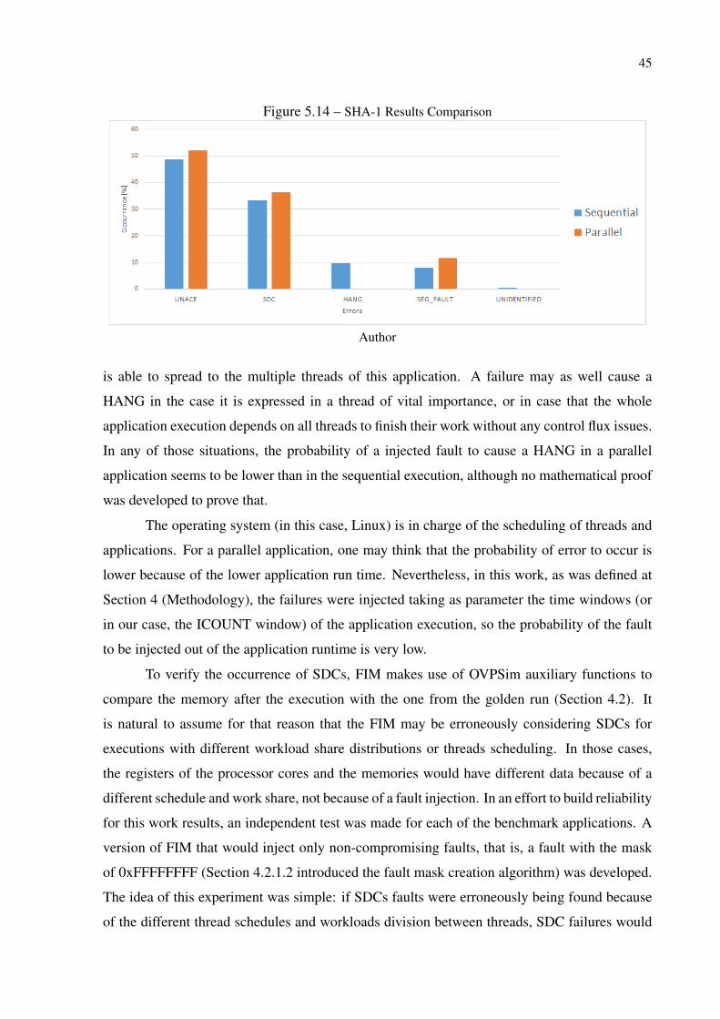
The comparison between the two versions of the SHA-1 algorithm is not impressive.

As Figure 5.14 shows, both versions have a very similar behavior under fault injection. An

interesting fact is the absence of HANG failures at the parallel execution. Once the workload is

divided into more than one worker - as defined by the parallel version specification at Section

4.3 - the occurrence of HANG failures is much lower (because the execution time is lower as

well).

Section 4.3 states that the parallelization strategy for SHA-1 is that of a master-slave.

None the less, a great part of the algorithm execution consists of work done by the master

thread. Just as is the case for the stringsearch benchmark, the program code of SHA-1 is the

same for the parallel and sequential versions of the execution, differing only by the number of

workers, which is a parameter passed as input for the application. Because the code of both

the versions are the same, and a big part of the executions is actually sequential (as the master

thread works are not executed in parallel), it is not astonishing that the parallel and sequential

executions have a similar result.

A very interesting fact arising from those analyzes is the augmentation of the SDC sen-

sitivity for every parallel execution when compared with it’s sequential associate (apart from

Susan).

The parallel versions of the algorithm also seem to be much less sensitive to HANG

failures. That may be explained by the parallelization itself. Once an application have more

than one flux of processing work, it is expected that a failure will only cause a HANG if it

45

Figure 5.14 – SHA-1 Results Comparison

Author

is able to spread to the multiple threads of this application. A failure may as well cause a

HANG in the case it is expressed in a thread of vital importance, or in case that the whole

application execution depends on all threads to finish their work without any control flux issues.

In any of those situations, the probability of a injected fault to cause a HANG in a parallel

application seems to be lower than in the sequential execution, although no mathematical proof

was developed to prove that.

The operating system (in this case, Linux) is in charge of the scheduling of threads and

applications. For a parallel application, one may think that the probability of error to occur is

lower because of the lower application run time. Nevertheless, in this work, as was defined at

Section 4 (Methodology), the failures were injected taking as parameter the time windows (or

in our case, the ICOUNT window) of the application execution, so the probability of the fault

to be injected out of the application runtime is very low.

To verify the occurrence of SDCs, FIM makes use of OVPSim auxiliary functions to

compare the memory after the execution with the one from the golden run (Section 4.2). It

is natural to assume for that reason that the FIM may be erroneously considering SDCs for

executions with different workload share distributions or threads scheduling. In those cases,

the registers of the processor cores and the memories would have different data because of a

different schedule and work share, not because of a fault injection. In an effort to build reliability

for this work results, an independent test was made for each of the benchmark applications. A

version of FIM that would inject only non-compromising faults, that is, a fault with the mask

of 0xFFFFFFFF (Section 4.2.1.2 introduced the fault mask creation algorithm) was developed.

The idea of this experiment was simple: if SDCs faults were erroneously being found because

of the different thread schedules and workloads division between threads, SDC failures would

46

be accused even while injecting faults with masks that would cause no bit to flip in the register.

The result of this experiment is rather satisfying. The injection of the non-compromising faults

had no influence on the application execution: 100% of the injected faults were captured by

FIM as UNACE. This supports even further the statement that FIM is a reliable fault injection

tool and is capable of rightfully classify the errors generated by the fault injection.

5.5 Register Coverage Analysis

Some interesting data can be extracted from another information available at our sim-

ulation results: the register failure coverage. In this work, register failure coverage is defined

as the percentage faults injected in a given register that have caused failures. For this analysis,

every failure was considered, except for the ones accused as Masked_Fault (see Section 4.4.1

for the definition). It is expected that some of the registers have lower sensitivity for failures,

because they may be of frequent use by Linux or any other system operation.

The following tables present the register coverage for each of the tests benchmarks and

for both the sequential and parallel versions of the algorithms.

Table 5.1 – Register Coverage for Fault Injection at DijkstraRegister Failure Cov. - Seq. Failure Cov. - Par. One Queue Failure Cov. - Par. N Queues

pc 100% 90% 100%

sp 100% 93% 92%

r0 52% 35% 30%

r1 30% 27% 22%

r2 53% 31% 11%

r3 35% 36% 26%

r4 55% 63% 39%

r5 88% 64% 50%

r6 70% 50% 58%

r7 75% 55% 45%

r8 53% 50% 52%

r9 48% 60% 50%

r10 76% 35% 56%

r11 80% 64% 66%

r12 22% 15% 23%

Table 5.1 shows the results for the Dijkstra algorithm. This table appears to indicate that

the pc and sp registers are the ones the most sensitive to failures. It was an expected finding,

once those are the most frequently used registers.

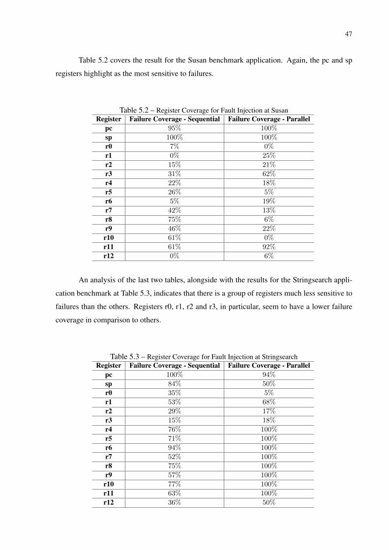
47

Table 5.2 covers the result for the Susan benchmark application. Again, the pc and sp

registers highlight as the most sensitive to failures.

Table 5.2 – Register Coverage for Fault Injection at SusanRegister Failure Coverage - Sequential Failure Coverage - Parallel

pc 95% 100%

sp 100% 100%

r0 7% 0%

r1 0% 25%

r2 15% 21%

r3 31% 62%

r4 22% 18%

r5 26% 5%

r6 5% 19%

r7 42% 13%

r8 75% 6%

r9 46% 22%

r10 61% 0%

r11 61% 92%

r12 0% 6%

An analysis of the last two tables, alongside with the results for the Stringsearch appli-

cation benchmark at Table 5.3, indicates that there is a group of registers much less sensitive to

failures than the others. Registers r0, r1, r2 and r3, in particular, seem to have a lower failure

coverage in comparison to others.

Table 5.3 – Register Coverage for Fault Injection at StringsearchRegister Failure Coverage - Sequential Failure Coverage - Parallel

pc 100% 94%

sp 84% 50%

r0 35% 5%

r1 53% 68%

r2 29% 17%

r3 15% 18%

r4 76% 100%

r5 71% 100%

r6 94% 100%

r7 52% 100%

r8 75% 100%

r9 57% 100%

r10 77% 100%

r11 63% 100%

r12 36% 50%

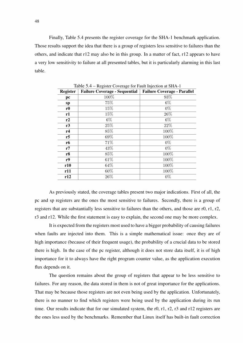
48

Finally, Table 5.4 presents the register coverage for the SHA-1 benchmark application.

Those results support the idea that there is a group of registers less sensitive to failures than the

others, and indicate that r12 may also be in this group. In a matter of fact, r12 appears to have

a very low sensitivity to failure at all presented tables, but it is particularly alarming in this last

table.

Table 5.4 – Register Coverage for Fault Injection at SHA-1Register Failure Coverage - Sequential Failure Coverage - Parallel

pc 100% 93%

sp 75% 6%

r0 15% 0%

r1 15% 26%

r2 6% 6%

r3 25% 22%

r4 85% 100%

r5 69% 100%

r6 71% 0%

r7 43% 0%

r8 85% 100%

r9 61% 100%

r10 64% 100%

r11 60% 100%

r12 26% 0%

As previously stated, the coverage tables present two major indications. First of all, the

pc and sp registers are the ones the most sensitive to failures. Secondly, there is a group of

registers that are substantially less sensitive to failures than the others, and those are r0, r1, r2,

r3 and r12. While the first statement is easy to explain, the second one may be more complex.

It is expected from the registers most used to have a bigger probability of causing failures

when faults are injected into them. This is a simple mathematical issue: once they are of

high importance (because of their frequent usage), the probability of a crucial data to be stored

there is high. In the case of the pc register, although it does not store data itself, it is of high

importance for it to always have the right program counter value, as the application execution

flux depends on it.

The question remains about the group of registers that appear to be less sensitive to

failures. For any reason, the data stored in them is not of great importance for the applications.

That may be because those registers are not even being used by the application. Unfortunately,

there is no manner to find which registers were being used by the application during its run

time. Our results indicate that for our simulated system, the r0, r1, r2, r3 and r12 registers are

the ones less used by the benchmarks. Remember that Linux itself has built-in fault correction

49

capabilities, so if those requisites are in any way reserved by the OS, or of preferential use of

Linux, it may be the cause of this behavior.

50

6 CONCLUSION

This work presented the software error analysis at the Zynq SoC ARM embedded pro-

cessor. It distinguishes itself from an ordinary software error analysis by making use of a pro-

cessor with two cores, and evaluating the results from sequential algorithms and parallel ones.

This study is important due to the high usability of the Zynq Soc at industrial and safety-critical

applications. The objective of this work was to map the failures generated by fault injection in

the applications normally developed for embedded processing.

Based in fault injection methods theoretically developed by works such as (HSUEH;

TSAI; IYER, 1997) and (ARLAT et al., 1990), it was possible to develop and adapt a fault

injector to suit the research’s needs and achieve the desired simulation environment. OVPSim

was of great use in this task, and proved itself to be a highly reliable and stable simulator, not to

mention the plethora of design and development tools it offers. Those tools were fundamental

to the good development of the fault injection method and simulation analysis.

Because of the characteristics of the simulation and fault injection system, it was not

possible to obtain measures such as the AVF and the SER with the tests results. This limita-

tion, nevertheless, is well expected when making use of simulation-based and software failure

injections, which was the case of this work.

As benchmarks, some applications from the ParmiBench benchmarks suit were used.

This suite contains applications that are generally used for industrial purposes and developed to

run on embedded processors. Being the Zynq SoC one of the most popular COTS systems used

for this finality, those benchmarks emulate the real life usage of the system resources, and the

algorithms peculiarities are valuable for this study. The ParmiBench suite proved itself a very

reliable set of applications for our testing objective. Nevertheless, some of those applications

were more computer-intensive than expected, and implied in long simulations run times, which

limited the number of executions used for evaluation.

As previously stated on other similar works, the simulation results imply that the sen-

sitivity to failures rely not only on the architecture of the device running the application, but

also on the application’s algorithm itself. Once the COTS SoCs used by industrial and safety-

critical projects usually focus on specific applications for an specific purpose (that is, they are

not general-purpose computers like the popular use), this work results demonstrate the impor-

tance of well knowing the application weakness to specific failures, so that it can be treated by

any fault tolerance method justifiable.

The final results also arise interesting ideas and subjects for future work. The analysis of

51

the Susan benchmarks, for instance, is an indication that certain parallelization algorithms may

introduce into the code a natural fault tolerance. Another interesting result from the analyses

is that they show a general tendency of augmentation of the application’s sensitivity to SDC

failures when running the parallel versions of algorithms. If that is to be proven to be a gen-

eral rule (which demands a more focused and intensive research), the development of special

fault tolerance techniques for parallel applications to protect them from SDCs would be greatly

justified, and a promising path for future works.

The results from the register failure coverage also arise as promising for future works.

This work did not analyze what types of failures each register tends to generate, which may be

interesting information. It is natural that registers of different use (such as sp and pc registers)

may cause different types of failures when subject to fault injection. This data may also help to

provide and develop special fault tolerance systems, according to each application’s necessities

and sensitivity to failures.

52

REFERENCES

ALDERIGHI, M. et al. Evaluation of single event upset mitigation schemes for sram basedfpgas using the flipper fault injection platform. In: IEEE. Defect and Fault-Tolerance inVLSI Systems, 2007. DFT’07. 22nd IEEE International Symposium on. [S.l.], 2007. p.105–113.

ALEXANDRESCU, D.; STERPONE, L.; LÓPEZ-ONGIL, C. Fault injection and faulttolerance methodologies for assessing device robustness and mitigating against ionizingradiation. 19th IEEE European Test Symposium (ETS), 2014.

ANDO, H. et al. A 1.3-ghz fifth-generation sparc64 microprocessor. Solid-State Circuits,IEEE Journal of, IEEE, v. 38, n. 11, p. 1896–1905, 2003.

ARLAT, J. et al. Fault injection for dependability validation: A methodology and someapplications. Software Engineering, IEEE Transactions on, IEEE, v. 16, n. 2, p. 166–182,1990.

CALIN, T.; NICOLAIDIS, M.; VELAZCO, R. Upset hardened memory design for submicroncmos technology. IEEE-Transactions-on-Nuclear-Science., p. 2874–8, 1996.

CLARK, J.; PRADHAN, D. K. et al. Fault injection: A method for validating computer-systemdependability. Computer, IEEE, v. 28, n. 6, p. 47–56, 1995.

CODERRE, P. et al. Introduction to ionizing radiation (pdf). MIT, 2006.

DODD, P.; MASSENGILL, L. Basic mechanisms and modeling of single-event upset in digitalmicroelectronics. Nuclear Science, IEEE Transactions on, v. 50, n. 3, p. 583–602, June 2003.ISSN 0018-9499.

DODD, P. E. et al. Neutron-induced latchup in srams at ground level. In: IEEE. ReliabilityPhysics Symposium Proceedings, 2003. 41st Annual. 2003 IEEE International. [S.l.],2003. p. 51–55.

EJLALI, A.; MIREMADI, S. G. Error propagation analysis using FPGA-based SEU-fault injection. Microelectronics Reliability, v. 48, n. 2, p. 319–328, 2008. ISSN00262714. Available from Internet: <http://www.sciencedirect.com/science/article/pii/S0026271407001746>.

FENG, S. et al. Shoestring: probabilistic soft error reliability on the cheap. In: ACM. ACMSIGARCH Computer Architecture News. [S.l.], 2010. v. 38, n. 1, p. 385–396.

FOUILLAT, P. et al. Investigation of single-event transients in fast integrated circuits with apulsed laser. International journal of high speed electronics and systems, World Scientific,v. 14, n. 02, p. 327–339, 2004.

HILDERMAN, V.; BAGHI, T. Avionics certification: a complete guide to DO-178(software), DO-254 (hardware). [S.l.]: Avionics Communications, 2007.

HSUEH, M.-C.; TSAI, T. K.; IYER, R. K. Fault injection techniques and tools. Computer,IEEE, v. 30, n. 4, p. 75–82, 1997.

53

IQBAL, S. M. Z.; LIANG, Y.; GRAHN, H. ParMiBench - An open-source benchmark forembedded multiprocessor systems. IEEE Computer Architecture Letters, v. 9, n. 2, p.45–48, 2010. ISSN 15566056.

KALBARCZYK, Z.; IYER, K. Characterization of linux kernel behavior under errors. 2003International Conference on Dependable Systems and Networks, 2003. Proceedings.,v. 00, n. ii, p. 459–468, 2003. Available from Internet: <http://ieeexplore.ieee.org/lpdocs/epic03/wrapper.htm?arnumber=1209956>.

KOGA, R. et al. Single event functional interrupt (sefi) sensitivity in microcircuits. In: IEEE.Radiation and Its Effects on Components and Systems, 1997. RADECS 97. FourthEuropean Conference on. [S.l.], 1997. p. 311–318.

MUKHERJEE, S. S.; KONTZ, M.; REINHARDT, S. K. Detailed design and evaluationof redundant multi-threading alternatives. In: IEEE. Computer Architecture, 2002.Proceedings. 29th Annual International Symposium on. [S.l.], 2002. p. 99–110.

MUKHERJEE, S. S. et al. A systematic methodology to compute the architecturalvulnerability factors for a high-performance microprocessor. In: IEEE COMPUTERSOCIETY. Proceedings of the 36th annual IEEE/ACM International Symposium onMicroarchitecture. [S.l.], 2003. p. 29.

ROSA, F. et al. A fast and scalable fault injection framework to evaluate multi/many-core softerror reliability. In: Defect and Fault Tolerance in VLSI and Nanotechnology Systems(DFTS), 2015 IEEE International Symposium on. [S.l.: s.n.], 2015. p. 211–214.

SANTINI, T. et al. Exploiting cache conflicts to reduce radiation sensitivity of operatingsystems on embedded systems. In: Compilers, Architecture and Synthesis for EmbeddedSystems (CASES), 2015 International Conference on. [S.l.: s.n.], 2015. p. 49–58.

VARGAS, V. et al. Evaluating seu fault-injection on parallel applications implemented onmulticore processors. In: Circuits Systems (LASCAS), 2015 IEEE 6th Latin AmericanSymposium on. [S.l.: s.n.], 2015. p. 1–4.

WOOD, A. Data integrity concepts, features, and technology. White paper, Tandem Division,Compaq Computer Corporation, 1999.