1

Introduction to Social Network MethodsTable of Contents

This page is the starting point for an on-line textbook supporting Sociology 157, anundergraduate introductory course on social network analysis. Robert A. Hanneman of theDepartment of Sociology teaches the course at the University of California, Riverside. Feel freeto use and reproduce this textbook (with citation). For more information, or to offer comments,you can send me e-mail.

About this Textbook

This on-line textbook introduces many of the basics of forma l approaches to the analysis ofsocial networks. It provides very brief overviews of a number of major areas with someexamples. The text relies heavily on the work of Freeman, Borgatti, and Everett (the authors ofthe UCINET software package). The materials here, and their organization, were also verystrongly influenced by the text of Wasserman and Faust, and by a graduate seminar conducted byProfessor Phillip Bonacich at UCLA in 1998. Errors and omissions, of course, are theresponsibility of the author.

Table of Contents

1. Social network data2. Why formal methods?3. Using graphs to represent social relations4. Using matrices to represent social relations5. Basic properties of networks and actors6. Centrality and power7. Cliques and sub-groups8. Network positions and social roles: The analysis of equivalence9. Structural equivalence10. Automorphic equivalence11. Regular equivalence

A bibliography of works about, or examples of, social network methods

2

1. Social Network Data

Introduction: What's different about social network data?

On one hand, there really isn't anything about social network data that is all that unusual.Networkers do use a specialized language for describing the structure and contents of the sets ofobservations that they use. But, network data can also be described and understood using theideas and concepts of more familiar methods, like cross-sectional survey research.

On the other hand, the data sets that networkers develop usually end up looking quite differentfrom the conventional rectangular data array so familiar to survey researchers and statisticalanalysts. The differences are quite important because they lead us to look at our data in adifferent way -- and even lead us to think differently about how to apply statistics.

"Conventional" sociological data consists of a rectangular array of measurements. The rows ofthe array are the cases, or subjects, or observations. The columns consist of scores (quantitativeor qualitative) on attributes, or variables, or measures. Each cell of the array then describes thescore of some actor on some attribute. In some cases, there may be a third dimension to thesearrays, representing panels of observations or multiple groups.

Name Sex Age In-Degree

Bob Male 32 2

Carol Female 27 1

Ted Male 29 1

Alice Female 28 3

The fundamental data structure is one that leads us to compare how actors are similar ordissimilar to each other across attributes (by comparing rows). Or, perhaps more commonly, weexamine how variables are similar or dissimilar to each other in their distributions across actors(by comparing or correlating columns).

"Network" data (in their purest form) consist of a square array of measurements. The rows of thearray are the cases, or subjects, or observations. The columns of the array are -- and note the keydifference from conventional data -- the same set of cases, subjects, or observations. In each cellof the array describes a relationship between the actors.

3

Who reports liking whom?

Choice:

Chooser: Bob Carol Ted Alice

Bob --- 0 1 1

Carol 1 --- 0 1

Ted 0 1 --- 1

Alice 1 0 0 ---

We could look at this data structure the same way as with attribute data. By comparing rows ofthe array, we can see which actors are similar to which other actors in whom they choose. Bylooking at the columns, we can see who is similar to whom in terms of being chosen by others.These are useful ways to look at the data, because they help us to see which actors have similarpositions in the network. This is the first major emphasis of network analysis: seeing how actorsare located or "embedded" in the overall network.

But a network analyst is also likely to look at the data structure in a second way -- holistically.The analyst might note that there are about equal numbers of ones and zeros in the matrix. Thissuggests that there is a moderate "density" of liking overall. The analyst might also compare thecells above and below the diagonal to see if there is reciprocity in choices (e.g. Bob chose Ted,did Ted choose Bob?). This is the second major emphasis of network analysis: seeing how thewhole pattern of individual choices gives rise to more holistic patterns.

It is quite possible to think of the network data set in the same terms as "conventional data." Onecan think of the rows as simply a listing of cases, and the columns as attributes of each actor (i.e.the relations with other actors can be thought of as "attributes" of each actor). Indeed, many ofthe techniques used by network analysts (like calculating correlations and distances) are appliedexactly the same way to network data as they would be to conventional data.

While it is possible to describe network data as just a special form of conventional data (and itis), network analysts look at the data in some rather fundamentally different ways. Rather thanthinking about how an actor's ties with other actors describes the attributes of "ego," networkanalysts instead see a structure of connections, within which the actor is embedded. Actors aredescribed by their relations, not by their attributes. And, the relations themselves are just asfundamental as the actors that they connect.

The major difference between conventional and network data is that conventional data focuseson actors and attributes; network data focus on actors and relations. The difference in emphasis isconsequential for the choices that a researcher must make in deciding on research design, in

4

conducting sampling, developing measurement, and handling the resulting data. It is not that theresearch tools used by network analysts are different from those of other social scientists (theymostly are not). But the special purposes and emphases of network research do call for somedifferent considerations.

In this chapter, we will take a look at some of the issues that arise in design, sampling, andmeasurement for social network analysis. Our discussion will focus on the two parts of networkdata: nodes (or actors) and edges (or relations). We will try to show some of the ways in whichnetwork data are similar to, and different from more familar actor by attribute data. We willintroduce some new terminology that makes it easier to describe the special features of networkdata. Lastly, we will briefly discuss how the differences between network and actor-attribute dataare consequential for the application of statistical tools.

Nodes

Network data are defined by actors and by relations (or nodes and ties, etc.). The nodes or actorspart of network data would seem to be pretty straight-forward. Other empirical approaches in thesocial sciences also think in terms of cases or subjects or sample elements and the like. There isone difference with most network data, however, that makes a big difference in how such dataare usually collected -- and the kinds of samples and populations that are studied.

Network analysis focuses on the relations among actors, and not individual actors and theirattributes. This means that the actors are usually not sampled independently, as in many otherkinds of studies (most typically, surveys). Suppose we are studying friendship ties, for example.John has been selected to be in our sample. When we ask him, John identifies seven friends. Weneed to track down each of those seven friends and ask them about their friendship ties, as well.The seven friends are in our sample because John is (and vice-versa), so the "sample elements"are no longer "independent."

The nodes or actors included in non-network studies tend to be the result of independentprobability sampling. Network studies are much more likely to include all of the actors whooccur within some (usually naturally occurring) boundary. Often network studies don't use"samples" at all, at least in the conventional sense. Rather, they tend to include all of the actors insome population or populations. Of course, the populations included in a network study may be asample of some larger set of populations. For example, when we study patterns of interactionamong students in classrooms, we include all of the children in a classroom (that is, we study thewhole population of the classroom). The classroom itself, though, might have been selected byprobability methods from a population of classrooms (say all of those in a school).

The use of whole populations as a way of selecting observations in (many) network studiesmakes it important for the analyst to be clear about the boundaries of each population to bestudied, and how individual units of observation are to be selected within that population.Network data sets also frequently involve several levels of analysis, with actors embedded at thelowest level (i.e. network designs can be described using the language of "nested" designs).

5

Populations, samples, and boundaries

Social network analysts rarely draw samples in their work. Most commonly, network analystswill identify some population and conduct a census (i.e. include all elements of the population asunits of observation). A network analyst might examine all of the nouns and objects occurring ina text, all of the persons at a birthday party, all members of a kinship group, of an organization,neighborhood, or social class (e.g. landowners in a region, or royalty).

Survey research methods usually use a quite different approach to deciding which nodes tostudy. A list is made of all nodes (sometimes stratified or clustered), and individual elements areselected by probability methods. The logic of the method treats each individual as a separate"replication" that is, in a sense, interchangeable with any other.

Because network methods focus on relations among actors, actors cannot be sampledindependently to be included as observations. If one actor happens to be selected, then we mustalso include all other actors to whom our ego has (or could have) ties. As a result, networkapproaches tend to study whole populations by means of census, rather than by sample (we willdiscuss a number of exceptions to this shortly, under the topic of sampling ties).

The populations that network analysts study are remarkably diverse. At one extreme, they mightconsist of symbols in texts or sounds in verbalizations; at the other extreme, nations in the worldsystem of states might constitute the population of nodes. Perhaps most common, of course, arepopulations of individual persons. In each case, however, the elements of the population to bestudied are defined by falling within some boundary.

The boundaries of the populations studied by network analysts are of two main types. Probablymost commonly, the boundaries are those imposed or created by the actors themselves. All themembers of a classroom, organization, club, neighborhood, or community can constitute apopulation. These are naturally occurring clusters, or networks. So, in a sense, social networkstudies often draw the boundaries around a population that is known, a priori, to be a network.Alternatively, a network analyst might take a more "demographic" or "ecological" approach todefining population boundaries. We might draw observations by contacting all of the people whoare found in a bounded spatial area, or who meet some criterion (having gross family incomesover $1,000,000 per year). Here, we might have reason to suspect that networks exist, but theentity being studied is an abstract aggregation imposed by the investigator -- rather than a patternof institutionalized social action that has been identified and labeled by it's participants.

Network analysts can expand the boundaries of their studies by replicating populations. Ratherthan studying one neighborhood, we can study several. This type of design (which could usesampling methods to select populations) allows for replication and for testing of hypotheses bycomparing populations. A second, and equally important way that network studies expand theirscope is by the inclusion of multiple levels of analysis, or modalities.

6

Modality and levels of analysis

The network analyst tends to see individual people nested within networks of face-to-facerelations with other persons. Often these networks of interpersonal relations become "socialfacts" and take on a life of their own. A family, for example, is a network of close relationsamong a set of people. But this particular network has been institutionalized and given a nameand reality beyond that of its component nodes. Individuals in their work relations may be seenas nested within organizations; in their leisure relations they may be nested in voluntaryassociations. Neighborhoods, communities, and even societies are, to varying degrees, socialentities in and of themselves. And, as social entities, they may form ties with the individualsnested within them, and with other social entities.

Often network data sets describe the nodes and relations among nodes for a single boundedpopulation. If I study the friendship patterns among students in a classroom, I am doing a studyof this type. But a classroom exists within a school - which might be thought of as a networkrelating classes and other actors (principals, administrators, librarians, etc.). And most schoolsexist within school districts, which can be thought of as networks of schools and other actors(school boards, research wings, purchasing and personnel departments, etc.). There may even bepatterns of ties among school districts (say by the exchange of students, teachers, curricularmaterials, etc.).

Most networkers think of individual persons as being embedded in networks that are embeddedin networks that are embedded in networks. Networkers describe such structures as "multi-modal." In our school example, individual students and teachers form one mode, classrooms asecond, schools a third, and so on. A data set that contains information about two types of socialentities (say persons and organizations) is a two mode network.

Of course, this kind of view of the nature of social structures is not unique to social networkers.Statistical analysts deal with the same issues as "hierarchical" or "nested" designs. Theoristsspeak of the macro-meso-micro levels of analysis, or develop schema for identifying levels ofanalysis (individual, group, organization, community, institution, society, global order beingperhaps the most commonly used system in sociology). One advantage of network thinking andmethod is that it naturally predisposes the analyst to focus on multiple levels of analysissimultaneously. That is, the network analyst is always interested in how the individual isembedded within a structure and how the structure emerges from the micro-relations betweenindividual parts. The ability of network methods to map such multi-modal relations is, at leastpotentially, a step forward in rigor.

Having claimed that social network methods are particularly well suited for dealing withmultiple levels of analysis and multi-modal data structures, it must immediately be admitted thatnetworkers rarely actually take much advantage. Most network analyses does move us beyondsimple micro or macro reductionism -- and this is good. Few, if any, data sets and analyses,however, have attempted to work at more than two modes simultaneously. And, even whenworking with two modes, the most common strategy is to examine them more or less separately

7

(one exception to this is the conjoint analysis of two mode networks).

Relations

The other half of the design of network data has to do with what ties or relations are to bemeasured for the selected nodes. There are two main issues to be discussed here. In manynetwork studies, all of the ties of a given type among all of the selected nodes are studied -- thatis, a census is conducted. But, sometimes different approaches are used (because they are lessexpensive, or because of a need to generalize) that sample ties. There is also a second kind ofsampling of ties that always occurs in network data. Any set of actors might be connected bymany different kinds of ties and relations (e.g. students in a classroom might like or dislike eachother, they might play together or not, they might share food or not, etc.). When we collectnetwork data, we are usually selecting, or sampling, from among a set of kinds of relations thatwe might have measured.

Sampling ties

Given a set of actors or nodes, there are several strategies for deciding how to go about collectingmeasurements on the relations among them. At one end of the spectrum of approaches are "fullnetwork" methods. This approach yields the maximum of information, but can also be costly anddifficult to execute, and may be difficult to generalize. At the other end of the spectrum aremethods that look quite like those used in conventional survey research. These approaches yieldconsiderably less information about network structure, but are often less costly, and often alloweasier generalization from the observations in the sample to some larger population. There is noone "right" method for all research questions and problems.

Full network methods require that we collect information about each actor's ties with all otheractors. In essence, this approach is taking a census of ties in a population of actors -- rather thana sample. For example we could collect data on shipments of copper between all pairs of nationstates in the world system from IMF records; we could examine the boards of directors of allpublic corporations for overlapping directors; we could count the number of vehicles movingbetween all pairs of cities; we could look at the flows of e-mail between all pairs of employees ina company; we could ask each child in a play group to identify their friends.

Because we collect information about ties between all pairs or dyads, full network data give acomplete picture of relations in the population. Most of the special approaches and methods ofnetwork analysis that we will discuss in the remainder of this text were developed to be usedwith full network data. Full network data is necessary to properly define and measure many ofthe structural concepts of network analysis (e.g. between-ness).

Full network data allows for very powerful descriptions and analyses of social structures.Unfortunately, full network data can also be very expensive and difficult to collect. Obtainingdata from every member of a population, and having every member rank or rate every othermember can be very challenging tasks in any but the smallest groups. The task is made moremanageable by asking respondents to identify a limited number of specific individuals withwhom they have ties. These lists can then be compiled and cross-connected. But, for large groups

8

(say all the people in a city), the task is practically impossible.

In many cases, the problems are not quite as severe as one might imagine. Most persons, groups,and organizations tend to have limited numbers of ties -- or at least limited numbers of strongties. This is probably because social actors have limited resources, energy, time, and cognativecapacity -- and cannot maintain large numbers of strong ties. It is also true that social structurescan develop a considerable degree of order and solidarity with relatively few connections.

Snowball methods begin with a focal actor or set of actors. Each of these actors is asked to namesome or all of their ties to other actors. Then, all the actors named (who were not part of theoriginal list) are tracked down and asked for some or all of their ties. The process continues untilno new actors are identified, or until we decide to stop (usually for reasons of time and resources,or because the new actors being named are very marginal to the group we are trying to study).

The snowball method can be particularly helpful for tracking down "special" populations (oftennumerically small sub-sets of people mixed in with large numbers of others). Business contactnetworks, community elites, deviant sub-cultures, avid stamp collectors, kinship networks, andmany other structures can be pretty effectively located and described by snowball methods. It issometimes not as difficult to achieve closure in snowball "samples" as one might think. Thelimitations on the numbers of strong ties that most actors have, and the tendency for ties to bereciprocated often make it fairly easy to find the boundaries.

There are two major potential limitations and weaknesses of snowball methods. First, actors whoare not connected (i.e. "isolates") are not located by this method. The presence and numbers ofisolates can be a very important feature of populations for some analytic purposes. The snowballmethod may tend to overstate the "connectedness" and "solidarity" of populations of actors.Second, there is no guaranteed way of finding all of the connected individuals in the population.Where does one start the snowball rolling? If we start in the wrong place or places, we may misswhole sub-sets of actors who are connected -- but not attached to our starting points.

Snowball approaches can be strengthened by giving some thought to how to select the initialnodes. In many studies, there may be a natural starting point. In community power studies, forexample, it is common to begin snowball searches with the chief executives of large economic,cultural, and political organizations. While such an approach will miss most of the community(those who are "isolated" from the elite network), the approach is very likely to capture the elitenetwork quite effectively.

Ego-centric networks (with alter connections)

In many cases it will not be possible (or necessary) to track down the full networks beginningwith focal nodes (as in the snowball method). An alternative approach is to begin with aselection of focal nodes (egos), and identify the nodes to which they are connected. Then, wedetermine which of the nodes identified in the first stage are connected to one another. This canbe done by contacting each of the nodes; sometimes we can ask ego to report which of the nodesthat it is tied to are tied to one another.

This kind of approach can be quite effective for collecting a form of relational data from very

9

large populations, and can be combined with attribute-based approaches. For example, we mighttake a simple random sample of male college students and ask them to report who are their closefriends, and which of these friends know one another. This kind of approach can give us a goodand reliable picture of the kinds of networks (or at least the local neighborhoods) in whichindividuals are embedded. We can find out such things as how many connections nodes have,and the extent to which these nodes are close-knit groups. Such data can be very useful inhelping to understand the opportunities and constraints that ego has as a result of the way theyare embedded in their networks.

The ego-centered approach with alter connections can also give us some information about thenetwork as a whole, though not as much as snowball or census approaches. Such data are, in fact,micro-network data sets -- samplings of local areas of larger networks. Many network properties-- distance, centrality, and various kinds of positional equivalence cannot be assessed with ego-centric data. Some properties, such as overall network density can be reasonably estimated withego-centric data. Some properties -- such as the prevailence of reciprocal ties, cliques, and thelike can be estimated rather directly.

Ego-centric networks (ego only)

Ego-centric methods really focus on the individual, rather than on the network as a whole. Bycollecting information on the connections among the actors connected to each focal ego, we canstill get a pretty good picture of the "local" networks or "neighborhoods" of individuals. Suchinformation is useful for understanding how networks affect individuals, and they also give a(incomplete) picture of the general texture of the network as a whole.

Suppose, however, that we only obtained information on ego's connections to alters -- but notinformation on the connections among those alters. Data like these are not really "network" dataat all. That is, they cannot be represented as a square actor-by-actor array of ties. But doesn'tmean that ego-centric data without connections among the alters are of no value for analystsseeking to take a structural or network approach to understanding actors. We can know, forexample, that some actors have many close friends and kin, and others have few. Knowing this,we are able to understand something about the differences in the actors places in social structure,and make some predictions about how these locations constrain their behavior. What we cannotknow from ego-centric data with any certainty is the nature of the macro-structure or the wholenetwork.

In ego-centric networks, the alters identified as connected to each ego are probably a set that isunconnected with those for each other ego. While we cannot assess the overall density orconnectedness of the population, we can sometimes be a bit more general. If we have some goodtheoretical reason to think about alters in terms of their social roles, rather than as individualoccupants of social roles, ego-centered networks can tell us a good bit about local socialstructures. For example, if we identify each of the alters connected to an ego by a friendshiprelation as "kin," "co-worker," "member of the same church," etc., we can build up a picture ofthe networks of social positions (rather than the networks of individuals) in which egos areembedded. Such an approach, of course, assumes that such categories as "kin" are real andmeaningful determinants of patterns of interaction.

10

Multiple relations

In a conventional actor-by-trait data set, each actor is described by many variables (and eachvariable is realized in many actors). In the most common social network data set of actor-by-actor ties, only one kind of relation is described. Just as we often are interested in multipleattributes of actors, we are often interested in multiple kinds of ties that connect actors in anetwork.

In thinking about the network ties among faculty in an academic department, for example, wemight be interested in which faculty have students in common, serve on the same committees,interact as friends outside of the workplace, have one or more areas of expertese in common, andco-author papers. The positions that actors hold in the web of group affiliations are multi-faceted.Positions in one set of relations may re-enforce or contradict positions in another (I might sharefriendship ties with one set of people with whom I do not work on committees, for example).Actors may be tied together closely in one relational network, but be quite distant from oneanother in a different relational network. The locations of actors in multi-relational networks andthe structure of networks composed of multiple relations are some of the most interesting (andstill relatively unexplored) areas of social network analysis.

When we collect social network data about certain kinds of relations among actors we are, in asense, sampling from a population of possible relations. Usually our research question and theoryindicate which of the kinds of relations among actors are the most relevant to our study, and wedo not sample -- but rather select -- relations. In a study concerned with economic dependencyand growth, for example, I could collect data on the exchange of performances by musiciansbetween nations -- but it is not really likely to be all that relevant.

If we do not know what relations to examine, how might we decide? There are a number ofconceptual approaches that might be of assistance. Systems theory, for example, suggests twodomains: material and informational. Material things are "conserved" in the sense that they canonly be located at one node of the network at a time. Movements of people betweenorganizations, money between people, automobiles between cities, and the like are all examplesof material things which move between nodes -- and hence establish a network of materialrelations. Informational things, to the systems theorist, are "non-conserved" in the sense that theycan be in more than one place at the same time. If I know something and share it with you, weboth now know it. In a sense, the commonality that is shared by the exchange of informationmay also be said to establish a tie between two nodes. One needs to be cautious here, however,not to confuse the simple possession of a common attribute (e.g. gender) with the presence of atie (e.g. the exchange of views between two persons on issues of gender).

Methodologies for working with multi-relational data are not as well developed as those forworking with single relations. Many interesting areas of work such as network correlation, multi-dimensional scaling and clustering, and role algebras have been developed to work with multi-relational data. For the most part, these topics are beyond the scope of the current text, and arebest approached after the basics of working with single relational networks are mastered.

11

Scales of measurement

Like other kinds of data, the information we collect about ties between actors can be measured(i.e. we can assign scores to our observations) at different "levels of measurement." The differentlevels of measurement are important because they limit the kinds of questions that can beexamined by the researcher. Scales of measurement are also important because different kinds ofscales have different mathematical properties, and call for different algorithms in describingpatterns and testing inferences about them.

It is conventional to distinguish nominal, ordinal, and interval levels of measurement (the ratiolevel can, for all practical purposes, be grouped with interval). It is useful, however, to furtherdivide nominal measurement into binary and multi-category variations; it is also useful todistinguish between full-rank ordinal measures and grouped ordinal measures. We will brieflydescribe all of these variations, and provide examples of how they are commonly applied insocial network studies.

Binary measures of relations: By far the most common approach to scaling (assigning numbersto) relations is to simply distinguish between relations being absent (coded zero), and ties beingpresent (coded one). If we ask respondents in a survey to tell us "which other people on this listdo you like?" we are doing binary measurement. Each person from the list that is selected iscoded one. Those who are not selected are coded zero.

Much of the development of graph theory in mathematics, and many of the algorithms formeasuring properties of actors and networks have been developed for binary data. Binary data isso widely used in network analysis that it is not unusual to see data that are measured at a"higher" level transformed into binary scores before analysis proceeds. To do this, one simplyselects some "cut point" and rescores cases as below the cutpoint (zero) or above it (one).Dichotomizing data in this way is throwing away information. The analyst needs to considerwhat is relevant (i.e. what is the theory about? is it about the presence and pattern of ties, orabout the strengths of ties?), and what algorithms are to be applied in deciding whether it isreasonable to recode the data. Very often, the additional power and simplicity of analysis ofbinary data is "worth" the cost in information lost.

Multiple-category nominal measures of relations: In collecting data we might ask ourrespondents to look at a list of other people and tell us: "for each person on this list, select thecategory that describes your relationship with them the best: friend, lover, business relationship,kin, or no relationship." We might score each person on the list as having a relationship of type"1" type "2" etc. This kind of a scale is nominal or qualitative -- each person's relationship to thesubject is coded by its type, rather than it's strength. Unlike the binary nominal (true-false) data,the multiple category nominal measure is multiple choice.

The most common approach to analyzing multiple-category nominal measures is to use it tocreate a series of binary measures. That is, we might take the data arising from the questiondescribed above and create separate sets of scores for friendship ties, for lover ties, for kin ties,

12

etc. This is very similar to "dummy coding" as a way of handling muliple choice types ofmeasures in statistical analysis. In examining the resulting data, however, one must rememberthat each node was allowed to have a tie in at most one of the resulting networks. That is, aperson can be a friendship tie or a lover tie -- but not both -- as a result of the way we asked thequestion. In examining the resulting networks, densities may be artificially low, and there will bean inherent negative correlation among the matrices.

This sort of multiple choice data can also be "binarized." That is, we can ignore what kind of tieis reported, and simply code whether a tie exists for a dyad, or not. This may be fine for someanalyses -- but it does waste information. One might also wish to regard the types of ties asreflecting some underlying continuous dimension (for example, emotional intensity). The typesof ties can then be scaled into a single grouped ordinal measure of tie strength. The scaling, ofcourse, reflects the predisposition of the analyst -- not the reports of the respondents.

Grouped ordinal measures of relations: One of the earliest traditions in the study of socialnetworks asked respondents to rate each of a set of others as "liked" "disliked" or "neutral." Theresult is a grouped ordinal scale (i.e., there can be more than one "liked" person, and thecategories reflect an underlying rank order of intensity). Usually, this kind of three-point scalewas coded -1, 0, and +1 to reflect negative liking, indifference, and positive liking. When scoredthis way, the pluses and minuses make it fairly easy to write algorithms that will count anddescribe various network properties (e.g. the structural balance of the graph).

Grouped ordinal measures can be used to reflect a number of different quantitative aspects ofrelations. Network analysts are often concerned with describing the "strength" of ties. But,"strength" may mean (some or all of) a variety of things. One dimension is the frequency ofinteraction -- do actors have contact daily, weekly, monthly, etc. Another dimension is"intensity," which usually reflects the degree of emotional arousal associated with therelationship (e.g. kin ties may be infrequent, but carry a high "emotional charge" because of thehighly ritualized and institutionalized expectations). Ties may be said to be stronger if theyinvolve many different contexts or types of ties. Summing nominal data about the presence orabsence of multiple types of ties gives rise to an ordinal (actually, interval) scale of onedimension of tie strength. Ties are also said to be stronger to the extent that they are reciprocated.Normally we would assess reciprocity by asking each actor in a dyad to report their feelingsabout the other. However, one might also ask each actor for their perceptions of the degree ofreciprocity in a relation: Would you say that neither of you like each other very much, that youlike X more than X likes you, that X likes you more than you like X, or that you both like eachother about equally?

Ordinal scales of measurement contain more information than nominal. That is, the scores reflectfiner gradations of tie strength than the simple binary "presence or absence." This would seem tobe a good thing, yet it is frequently difficult to take advantage of ordinal data. The mostcommonly used algorithms for the analysis of social networks have been designed for binarydata. Many have been adapted to continuous data -- but for interval, rather than ordinal scales ofmeasurement. Ordinal data, consequently, are often binarized by choosing some cut-point andrescoring. Alternatively, ordinal data are sometimes treated as though they really were interval.The former strategy has some risks, in that choices of cutpoints can be consequential; the latter

13

strategy has some risks, in that the intervals separating points on an ordinal scale may be veryheterogeneous.

Full-rank ordinal measures of relations: Sometimes it is possible to score the strength of all ofthe relations of an actor in a rank order from strongest to weakest. For example, I could ask eachrespondent to write a "1" next to the name of the person in the class that you like the most, a "2"next to the name of the person you like next most, etc. The kind of scale that would result fromthis would be a "full rank order scale." Such scales reflect differences in degree of intensity, butnot necessarily equal differences -- that is, the difference between my first and second choices isnot necessarily the same as the difference between my second and third choices. Each relation,however, has a unique score (1st, 2nd, 3rd, etc.).

Full rank ordinal measures are somewhat uncommon in the social networks research literature, asthey are in most other traditions. Consequently, there are relatively few methods, definitions, andalgorithms that take specific and full advantage of the information in such scales. Mostcommonly, full rank ordinal measures are treated as if they were interval. There is probablysomewhat less risk in treating fully rank ordered measures (compared to grouped ordinalmeasures) as though they were interval, though the assumption is still a risky one. Of course, it isalso possible to group the rank order scores into groups (i.e. produce a grouped ordinal scale) ordichotomize the data (e.g. the top three choices might be treated as ties, the remainder as non-ties). In combining information on multiple types of ties, it is frequently necessary to simplifyfull rank order scales. But, if we have a number of full rank order scales that we may wish tocombine to form a scale (i.e. rankings of people's likings of other in the group, frequency ofinteraction, etc.), the sum of such scales into an index is plausibly treated as a truly intervalmeasure.

Interval measures of relations: The most "advanced" level of measurement allows us todiscriminate among the relations reported in ways that allow us to validly state that, for example,"this tie is twice as strong as that tie." Ties are rated on scales in which the difference between a"1" and a "2" reflects the same amount of real difference as that between "23" and "24."

True interval level measures of the strength of many kinds of relationships are fairly easy toconstruct, with a little imagination and persistence. Asking respondents to report the details ofthe frequency or intensity of ties by survey or interview methods, however, can be ratherunreliable -- particularly if the relationships being tracked are not highly salient and infrequent.Rather than asking whether two people communicate, one could count the number of email,phone, and inter-office mail deliveries between them. Rather than asking whether two nationstrade with one another, look at statistics on balances of payments. In many cases, it is possible toconstruct interval level measures of relationship strength by using artifacts (e.g. statisticscollected for other purposes) or observation.

Continuous measures of the strengths of relationships allow the application of a wider range ofmathematical and statistical tools to the exploration and analysis of the data. Many of thealgorithms that have been developed by social network analysts, originally for binary data, havebeen extended to take advantage of the information available in full interval measures. Wheneverpossible, connections should be measured at the interval level -- as we can always move to a less

14

refined approach later; if data are collected at the nominal level, it is much more difficult tomove to a more refined level.

Even though it is a good idea to measure relationship intensity at the most refined level possible,most network analysis does not operate at this level. The most powerful insights of networkanalysis, and many of the mathematical and graphical tools used by network analysts weredeveloped for simple graphs (i.e. binary, undirected). Many characterizations of theembeddedness of actors in their networks, and of the networks themselves are most commonlythought of in discrete terms in the research literature. As a result, it is often desirable to reduceeven interval data to the binary level by choosing a cutting -point, and coding tie strength abovethat point as "1" and below that point as "0." Unfortunately, there is no single "correct" way tochoose a cut-point. Theory and the purposes of the analysis provide the best guidance.Sometimes examining the data can help (maybe the distribution of tie strengths really isdiscretely bi-modal, and displays a clear cut point; maybe the distribution is highly skewed andthe main feature is a distinction between no tie and any tie). When a cut-point is chosen, it iswise to also consider alternative values that are somewhat higher and lower, and repeat theanalyses with different cut-points to see if the substance of the results is affected. This can bevery tedious, but it is very necessary. Otherwise, one may be fooled into thinking that a realpattern has been found, when we have only observed the consequences of where we decided toput our cut-point.

A note on statistics and social network data

Social network analysis is more a branch of "mathematical" sociology than of "statistical orquantitative analysis," though networkers most certainly practice both approaches. Thedistinction between the two approaches is not clear cut. Mathematical approaches to networkanalysis tend to treat the data as "deterministic." That is, they tend to regard the measuredrelationships and relationship strengths as accurately reflecting the "real" or "final" or"equilibrium" status of the network. Mathematical types also tend to assume that theobservations are not a "sample" of some larger population of possible observations; rather, theobservations are usually regarded as the population of interest. Statistical analysts tend to regardthe particular scores on relationship strengths as stochastic or probabilistic realizations of anunderlying true tendency or probability distribution of relationship strengths. Statistical analystsalso tend to think of a particular set of network data as a "sample" of a larger class or populationof such networks or network elements -- and have a concern for the results of the current studywould be reproduced in the "next" study of similar samples.

In the chapters that follow in this text, we will mostly be concerned with the "mathematical"rather than the "statistical" side of network analysis (again, it is important to remember that I amover-drawing the differences in this discussion). Before passing on to this, we should note acouple main points about the relationship between the material that you will be studying here,and the main statistical approaches in sociology.

In one way, there is little apparent difference between conventional statistical approaches andnetwork approaches. Univariate, bi-variate, and even many multivariate descriptive statisticaltools are commonly used in the describing, exploring, and modeling social network data. Social

15

network data are, as we have pointed out, easily represented as arrays of numbers -- just likeother types of sociological data. As a result, the same kinds of operations can be performed onnetwork data as on other types of data. Algorithms from statistics are commonly used to describecharacteristics of individual observations (e.g. the median tie strength of actor X with all otheractors in the network) and the network as a whole (e.g. the mean of all tie strengths among allactors in the network). Statistical algorithms are very heavily used in assessing the degree ofsimilarity among actors, and if finding patterns in network data (e.g. factor analysis, clusteranalysis, multi-dimensional scaling). Even the tools of predictive modeling are commonlyapplied to network data (e.g. correlation and regression).

Descriptive statistical tools are really just algorithms for summarizing characteristics of thedistributions of scores. That is, they are mathematical operations. Where statistics really become"statistical" is on the inferential side. That is, when our attention turns to assessing thereproducibility or likelihood of the pattern that we have described. Inferential statistics can be,and are, applied to the analysis of network data. But, there are some quite important differencesbetween the flavors of inferential statistics used with network data, and those that are mostcommonly taught in basic courses in statistical analysis in sociology.

Probably the most common emphasis in the application of inferential statistics to social sciencedata is to answer questions about the stability, reproducibility, or generalizability of resultsobserved in a single sample. The main question is: if I repeated the study on a different sample(drawn by the same method), how likely is it that I would get the same answer about what isgoing on in the whole population from which I drew both samples? This is a really importantquestion -- because it helps us to assess the confidence (or lack of it) that we ought to have inassessing our theories and giving advice.

To the extent the observations used in a network analysis are drawn by probability samplingmethods from some identifiable population of actors and/or ties, the same kind of question aboutthe generalizability of sample results applies. Often this type of inferential question is of littleinterest to social network researchers. In many cases, they are studying a particular network orset of networks, and have no interest in generalizing to a larger population of such networks(either because there isn't any such population, or we don't care about generalizing to it in anyprobabilistic way). In some other cases we may have an interest in generalizing, but our samplewas not drawn by probability methods. Network analysis often relies on artifacts, directobservation, laboratory experiments, and documents as data sources -- and usually there are noplausible ways of identifying populations and drawing samples by probability methods.

The other major use of inferential statistics in the social sciences is for testing hypotheses. Inmany cases, the same or closely related tools are used for questions of assessing generalizabilityand for hypothesis testing. The basic logic of hypothesis testing is to compare an observed resultin a sample to some null hypothesis value, relative to the sampling variability of the result underthe assumption that the null hypothesis is true. If the sample result differs greatly from what waslikely to have been observed under the assumption that the null hypothesis is true -- then the nullhypothesis is probably not true.

The key link in the inferential chain of hypothesis testing is the estimation of the standard errors

16

of statistics. That is, estimating the expected amount that the value a statistic would "jumparound" from one sample to the next simply as a result of accidents of sampling. We rarely, ofcourse, can directly observe or calculate such standard errors -- because we don't havereplications. Instead, information from our sample is used to estimate the sampling variability.

With many common statistical procedures, it is possible to estimate standard errors by wellvalidated approximations (e.g. the standard error of a mean is usually estimated by the samplestandard deviation divided by the square root of the sample size). These approximations,however, hold when the observations are drawn by independent random sampling. Networkobservations are almost always non-independent, by definition. Consequently, conventionalinferential formulas do not apply to network data (though formulas developed for other types ofdependent sampling may apply). It is particularly dangerous to assume that such formulas doapply, because the non-independence of network observations will usually result in under-estimates of true sampling variability -- and hence, too much confidence in our results.

The approach of most network analysts interested in statistical inference for testing hypothesesabout network properties is to work out the probability distributions for statistics directly. Thisapproach is used because: 1) no one has developed approximations for the sampling distributionsof most of the descriptive statistics used by network analysts and 2) interest often focuses on theprobability of a parameter relative to some theoretical baseline (usually randomness) rather thanon the probability that a given network is typical of the population of all networks.

Suppose, for example, that I was interested in the proportion of the actors in a network who weremembers of cliques (or any other network statistic or parameter). The notion of a clique impliesstructure -- non-random connections among actors. I have data on a network of ten nodes, inwhich there are 20 symmetric ties among actors, and I observe that there is one clique containingfour actors. The inferential question might be posed as: how likely is it, if ties among actors werepurely random events, that a network composed of ten nodes and 20 symmetric ties woulddisplay one or more cliques of size four or more? If it turns out that cliques of size four or morein random networks of this size and degree are quite common, I should be very cautious inconcluding that I have discovered "structure" or non-randomness. If it turns out that such cliques(or more numerous or more inclusive ones) are very unlikely under the assumption that ties arepurely random, then it is very plausible to reach the conclusion that there is a social structurepresent.

But how can I determine this probability? The method used is one of simulation -- and, like mostsimulation, a lot of computer resources and some programming skills are often necessary. In thecurrent case, I might use a table of random numbers to distribute 20 ties among 10 actors, andthen search the resulting network for cliques of size four or more. If no clique is found, I record azero for the trial; if a clique is found, I record a one. The rest is simple. Just repeat theexperiment several thousand times and add up what proportion of the "trials" result in"successes." The probability of a success across these simulation experiments is a good estimatorof the likelihood that I might find a network of this size and density to have a clique of this size"just by accident" when the non-random causal mechanisms that I think cause cliques are not, infact, operating.

17

This may sound odd, and it is certainly a lot of work (most of which, thankfully, can be done bycomputers). But, in fact, it is not really different from the logic of testing hypotheses with non-network data. Social network data tend to differ from more "conventional" survey data in somekey ways: network data are often not probability samples, and the observations of individualnodes are not independent. These differences are quite consequential for both the questions ofgeneralization of findings, and for the mechanics of hypothesis testing. There is, however,nothing fundamentally different about the logic of the use of descriptive and inferential statisticswith social network data.

The application of statistics to social network data is an interesting area, and one that is, at thetime of this writing, at a "cutting edge" of research in the area. Since this text focuses on morebasic and commonplace uses of network analysis, we won't have very much more to say aboutstatistics beyond this point. You can think of much of what follows here as dealing with the"descriptive" side of statistics (developing index numbers to describe certain aspects of thedistribution of relational ties among actors in networks). For those with an interest in theinferential side, a good place to start is with the second half of the excellent Wasserman andFaust textbook.

18

2. Why Formal Methods?

Introduction to chapter 2

The basic idea of a social network is very simple. A social network is a set of actors (or points, ornodes, or agents) that may have relationships (or edges, or ties) with one another. Networks canhave few or many actors, and one or more kinds of relations between pairs of actors. To build auseful understanding of a social network, a complete and rigorous description of a pattern ofsocial relationships is a necessary starting point for analysis. That is, ideally we will know aboutall of the relationships between each pair of actors in the population.

One reason for using mathematical and graphical techniques in social network analysis is torepresent the descriptions of networks compactly and systematically. This also enables us to usecomputers to store and manipulate the information quickly and more accurately than we can byhand. For small populations of actors (e.g. the people in a neighborhood, or the business firms inan industry), we can describe the pattern of social relationships that connect the actors rathercompletely and effectively using words. To make sure that our description is complete, however,we might want to list all logically possible pairs of actors, and describe each kind of possiblerelationship for each pair. This can get pretty tedious if the number of actors and/or number ofkinds of relations is large. Formal representations ensure that all the necessary information issystematically represented, and provides rules for doing so in ways that are much more efficientthan lists.

A related reason for using (particularly mathematical) formal methods for representing socialnetworks is that mathematical representations allow us to apply computers to the analysis ofnetwork data. Why this is important will become clearer as we learn more about how structuralanalysis of social networks occurs. Suppose, for a simple example, that we had informationabout trade-flows of 50 different commodities (e.g. coffee, sugar, tea, copper, bauxite) amongthe 170 or so nations of the world system in a given year. Here, the 170 nations can be thought ofas actors or nodes, and the amount of each commodity exported from each nation to each of theother 169 can be thought of as the strength of a directed tie from the focal nation to the other. Asocial scientist might be interested in whether the "structures" of trade in mineral products aremore similar to one another than, the structure of trade in mineral products are to vegetableproducts. To answer this fairly simple (but also pretty important) question, a huge amount ofmanipulation of the data is necessary. It could take, literally, years to do by hand. It can be doneby a computer in a few minutes.

The third, and final reason for using "formal" methods (mathematics and graphs) for representingsocial network data is that the techniques of graphing and the rules of mathematics themselvessuggest things that we might look for in our data — things that might not have occurred to us ifwe presented our data using descriptions in words. Again, allow me a simple example.

Suppose we were describing the structure of close friendship in a group of four people: Bob,Carol, Ted, and Alice. This is easy enough to do with words. Suppose that Bob likes Carol and

19

Ted, but not Alice; Carol likes Ted, but neither Bob nor Alice; Ted likes all three of the othermembers of the group; and Alice likes only Ted (this description should probably strike you asbeing a description of a very unusual social structure).

We could also describe this pattern of liking ties with an actor-by-actor matrix where the rowsrepresent choices by each actor. We will put in a "1" if an actor likes another, and a "0" if theydon't. Such a matrix would look like:

Bob Carol Ted Alice

Bob --- 1 1 0

Carol 0 --- 1 0

Ted 1 1 --- 1

Alice 0 0 1 ---

There are lots of things that might immediately occur to us when we see our data arrayed in thisway, that we might not have thought of from reading the description of the pattern of ties inwords. For example, our eye is led to scan across each row; we notice that Ted likes more peoplethan Bob, than Alice and Carol. Is it possible that there is a pattern here? Are men are morelikely to report ties of liking than women are (actually, research literature suggests that this is notgenerally true). Using a "matrix representation" also immediately raises a question: the locationson the main diagonal (e.g. Bob likes Bob, Carol likes Carol) are empty. Is this a reasonablething? Or, should our description of the pattern of liking in the group include some statementsabout "self-liking"? There isn't any right answer to this question. My point is just that using amatrix to represent the pattern of ties among actors may let us see some patterns more easily, andmay cause us to ask some questions (and maybe even some useful ones) that a verbal descriptiondoesn't stimulate.

Summary of chapter 2

There are three main reasons for using "formal" methods in representing social network data:

Matrices and graphs are compact and systematic.They summarize and present a lot of information quickly and easily; and they force us to besystematic and complete in describing patterns of social relations.

Matrices and graphs allow us to apply computers to analyzing data.This is helpful because doing systematic analysis of social network data can be extremely tediousif the number of actors or number of types of relationships among the actors is large. Most of thework is dull, repetitive, and uninteresting, but requires accuracy. This is exactly the sort of thing

20

that computers do well, and we don't.

Matrices and graphs have rules and conventions.Sometimes these are just rules and conventions that help us communicate clearly. But sometimesthe rules and conventions of the language of graphs and mathematics themselves lead us to seethings in our data that might not have occurred to us to look for if we had described our data onlywith words.

So, we need to learn the basics of representing social network data using matrices and graphs.That's what the next chapter is about.

21

3. Using Graphs to Represent Social Relations

Introduction: Representing Networks with Graphs

Social network analysts use two kinds of tools from mathematics to represent information aboutpatterns of ties among social actors: graphs and matrices. On this page, we will learn enoughabout graphs to understand how to represent social network data. On the next page, we will lookat matrix representations of social relations. With these tools in hand, we can understand most ofthe things that network analysts do with such data (for example, calculate precise measures of"relative density of ties").

There is a lot more to these topics than we will cover here; mathematics has whole sub-fieldsdevoted to "graph theory" and to "matrix algebra." Social scientists have borrowed just a fewthings that they find helpful for describing and analyzing patterns of social relations.

A word of warning: there is a lot of specialized terminology here that you do need to learn. It'sworth the effort, because we can represent some important ideas about social structure in quitesimple ways, once the basics have been mastered.

Graphs and Sociograms

There are lots of different kinds of "graphs." Bar charts, pie charts, line and trend charts, andmany other things are called graphs and/or graphics. Network analysis uses (primarily) one kindof graphic display that consists of points (or nodes) to represent actors and lines (or edges) torepresent ties or relations. When sociologists borrowed this way of graphing things from themathematicians, they re-named their graphics "sociograms." Mathematicians know the kind ofgraphic displays by the names of "directed graphs" "signed graphs" or simply "graphs."

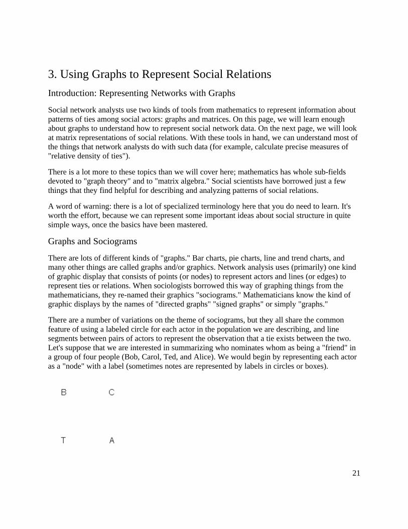
There are a number of variations on the theme of sociograms, but they all share the commonfeature of using a labeled circle for each actor in the population we are describing, and linesegments between pairs of actors to represent the observation that a tie exists between the two.Let's suppose that we are interested in summarizing who nominates whom as being a "friend" ina group of four people (Bob, Carol, Ted, and Alice). We would begin by representing each actoras a "node" with a label (sometimes notes are represented by labels in circles or boxes).

22

We collected our data about friendship ties by asking each member of the group (privately andconfidentially) who they regarded as "close friends" from a list containing each of the othermembers of the group. Each of the four people could choose none to all three of the others as"close friends." As it turned out, in our (fictitious) case, Bob chose Carol and Ted, but not Alice;Carol chose only Ted; Ted chose Bob and Carol and Alice; and Alice chose only Ted. We wouldrepresent this information by drawing an arrow from the chooser to each of the chosen, as in thenext graph:

Kinds of Graphs

Now we need to introduce some terminology to describe different kinds of graphs. Thisparticular example above is a binary (as opposed to a signed or ordinal or valued) and directed(as opposed to a co-occurrence or co-presence or bonded-tie) graph. The social relations beingdescribed here are also simplex (as opposed to multiplex).

Levels of Measurement: Binary, Signed, and Valued Graphs

In describing the pattern of who describes whom as a close friend, we could have asked ourquestion in several different ways. If we asked each respondent "is this person a close friend ornot," we are asking for a binary choice: each person is or is not chosen by each interviewee.Many social relationships can be described this way: the only thing that matters is whether a tieexists or not. When our data are collected this way, we can graph them simply: an arrowrepresents a choice that was made, no arrow represents the absence of a choice. But, we couldhave asked the question a second way: "for each person on this list, indicate whether you like,dislike, or don't care." We might assign a + to indicate "liking," zero to indicate "don't care" and -to indicate dislike. This kind of data is called "signed" data. The graph with signed data uses a +on the arrow to indicate a positive choice, a - to indicate a negative choice, and no arrow toindicate neutral or indifferent. Yet another approach would have been to ask: "rank the threepeople on this list in order of who you like most, next most, and least." This would give us "rankorder" or "ordinal" data describing the strength of each friendship choice. Lastly, we could haveasked: "on a scale from minus one hundred to plus one hundred - where minus 100 means youhate this person, zero means you feel neutral, and plus 100 means you love this person - how doyou feel about...". This would give us information about the value of the strength of each choiceon a (supposedly, at least) ratio level of measurement. With either an ordinal or valued graph, wewould put the measure of the strength of the relationship on the arrow in the diagram.

23

Directed or "Bonded" Ties in the Graph

In our example, we asked each member of the group to choose which others in the group theyregarded as close friends. Each person (ego) then is being asked about ties or relations that theythemselves direct toward others (alters). Each alter does not necessarily feel the same way abouteach tie as ego does: Bob may regard himself as a good friend to Alice, but Alice does notnecessarily regard Bob as a good friend. It is very useful to describe many social structures asbeing composed of "directed" ties (which can be binary, signed, ordered, or valued). Indeed,most social processes involve sequences of directed actions. For example, suppose that person Adirects a comment to B, then B directs a comment back to A, and so on. We may not know theorder in which actions occurred (i.e. who started the conversation), or we may not care. In thisexample, we might just want to know that "A and B are having a conversation." In this case, thetie or relation "in conversation with" necessarily involves both actors A and B. Both A and B are"co-present" or "co-occurring" in the relation of "having a conversation." Or, we might alsodescribe the situation as being one of an the social institution of a "conversation" that bydefinition involves two (or more) actors "bonded" in an interaction (Berkowitz).

"Directed" graphs use the convention of connecting nodes or actors with arrows that havearrowheads, indicating who is directing the tie toward whom. This is what we used in the graphsabove, where individuals (egos) were directing choices toward others (alters). "Co-occurrence"or "co-presence" or "bonded-tie" graphs use the convention of connecting the pair of actorsinvolved in the relation with a simple line segment (no arrowhead). Be careful here, though. In adirected graph, Bob could choose Ted, and Ted choose Bob. This would be represented byheaded arrows going from Bob to Ted, and from Ted to Bob, or by a double-headed arrow. But,this represents a different meaning from a graph that shows Bob and Ted connected by a singleline segment without arrowheads. Such a graph would say "there is a relationship called closefriend which ties Bob and Ted together." The distinction can be subtle, but it is important insome analyses.

Simplex or Multiplex Relations in the Graph

The information that we have represented about the social structure of our group of four peopleis pretty simple. That is, it describes only one type of tie or relation - choice of a close friend. Agraph that represents a single kind of relation is called a simplex graph. Social structures,however, are often multiplex. That is, there are multiple different kinds of ties among socialactors. Let's add a second kind of relation to our example. In addition to friendship choices, letsalso suppose that we asked each person whether they are kinfolk of each of the other three. Bobidentifies Ted as kin; Ted identifies Bob; and Ted and Alice identify one another (the full storyhere might be that Bob and Ted are brothers, and Ted and Alice are spouses). We could add thisinformation to our graph, using a different color or different line style to represent the secondtype of relation ("is kin of...").

We can see that the second kind of tie, "kinship" re-enforces the strength of the relationshipsbetween Bob and Ted and between Ted and Alice (or, perhaps, the presence of a kinship tieexplains the mutual choices as good friends). The reciprocated friendship tie between Carol andTed, however, is different, because it is not re-enforced by a kinship bond.

24

Of course, if we were examining many different kinds of relationships among the same set ofactors, putting all of this information into a single graph might make it too difficult to read, so wemight, instead, use multiple graphs with the actors in the same locations in each. We might alsowant to represent the multiplexity of the data in some simpler way. We could use lines ofdifferent thickness to represent how many ties existed between each pair of actors; or we couldcount the number of relations that were present for each pair and use a valued graph.

Summary of chapter 3

A graph (sometimes called a sociogram) is composed of nodes (or actors or points) connected byedges (or relations or ties). A graph may represent a single type of relations among the actors(simplex), or more than one kind of relation (multiplex). Each tie or relation may be directed (i.e.originates with a source actor and reaches a target actor), or it may be a tie that represents co-occurrence, co-presence, or a bonded-tie between the pair of actors. Directed ties are representedwith arrows, bonded-tie relations are represented with line segments. Directed ties may bereciprocated (A chooses B and B chooses A); such ties can be represented with a double-headedarrow. The strength of ties among actors in a graph may be nominal or binary (representspresence or absence of a tie); signed (represents a negative tie, a positive tie, or no tie); ordinal(represents whether the tie is the strongest, next strongest, etc.); or valued (measured on aninterval or ratio level). In speaking the position of one actor or node in a graph to other actors ornodes in a graph, we may refer to the focal actor as "ego" and the other actors as "alters."

Review questions for chapter 3

1. What are "nodes" and "edges"? In a sociogram, what is used for nodes? for edges?

2. How do valued, binary, and signed graphs correspond to the "nominal" "ordinal" and"interval" levels of measurement?

3. Distinguish between directed relations or ties and "bonded" relations or ties.

4. How does a reciprocated directed relation differ from a "bonded" relation?

5. Give and example of a multi-plex relation. How can multi-plex relations be represented ingraphs?

Application questions for chapter 3

1. Think of the readings from the first part of the course. Did any studies present graphs? If theydid, what kinds of graphs were they (that is, what is the technical description of the kind of graphor matrix). Pick one article and show what a graph of its data would look like.

2. Suppose that I was interested in drawing a graph of which large corporations were networkedwith one another by having the same persons on their boards of directors. Would it make moresense to use "directed" ties, or "bonded" ties for my graph? Can you think of a kind of relationamong large corporations that would be better represented with directed ties?

3. Think of some small group of which you are a member (maybe a club, or a set of friends, or

25

people living in the same apartment complex, etc.). What kinds of relations among them mighttell us something about the social structures in this population? Try drawing a graph to representone of the kinds of relations you chose. Can you extend this graph to also describe a second kindof relation? (e.g. one might start with "who likes whom?" and add "who spends a lot of time withwhom?").

4. Make graphs of a "star" network, a "line," and a "circle." Think of real world examples ofthese kinds of structures where the ties are directed and where they are bonded, or undirected.What does a strict hierarchy look like? What does a population that is segregated into two groupslook like?

26

4. Using Matrices to Represent Social Relations

Introduction to chapter 4

Graphs are very useful ways of presenting information about social networks. However, whenthere are many actors and/or many kinds of relations, they can become so visually complicatedthat it is very difficult to see patterns. It is also possible to represent information about socialnetworks in the form of matrices. Representing the information in this way also allows theapplication of mathematical and computer tools to summarize and find patterns. Social networkanalysts use matrices in a number of different ways. So, understanding a few basic things aboutmatrices from mathematics is necessary. We'll go over just a few basics here that cover most ofwhat you need to know to understand what social network analysts are doing. For those whowant to know more, there are a number of good introductory books on matrix algebra for socialscientists.

What is a Matrix?

To start with, a matrix is nothing more than a rectangular arrangement of a set of elements(actually, it's a bit more complicated than that, but we will return to matrices of more than twodimensions in a little bit). Rectangles have sizes that are described by the number of rows ofelements and columns of elements that they contain. A "3 by 6" matrix has three rows and sixcolumns; an "I by j" matrix has I rows and j columns. Here are empty 2 by 4 and 4 by 2 matrices:

2 by 4

1,1 1,2 1,3 1,4

2,1 2,2 2,3 2,4

4 by 2

1,1 1,2

2,1 2,2

3,1 3,2

4,1 4,2

27

The elements of a matrix are identified by their "addresses." Element 1,1 is the entry in the firstrow and first column; element 13,2 is in the 13th row and is the second element of that row. Thecell addresses have been entered as matrix elements in the two examples above. Matrices areoften represented as arrays of elements surrounded by vertical lines at their left and right, orsquare brackets at the left and right. In html (the language used to prepare web pages) it is easierto use "tables" to represent matrices. Matrices can be given names; these names are usuallypresented as capital bold-faced letters. Social scientists using matrices to represent socialnetworks often dispense with the mathematical conventions, and simply show their data as anarray of labeled rows and columns. The labels are not really part of the matrix, but are simply forclarity of presentation. The matrix below, for example, is a 4 by 4 matrix, with additional labels:

Bob Carol Ted Alice

Bob --- 1 0 0

Carol 1 --- 1 0

Ted 1 1 --- 1

Alice 0 0 1 ---

The "Adjacency" Matrix

The most common form of matrix in social network analysis is a very simple one composed of asmany rows and columns as there are actors in our data set, and where the elements represent theties between the actors. The simplest and most common matrix is binary. That is, if a tie ispresent, a one is entered in a cell; if there is no tie, a zero is entered. This kind of a matrix is thestarting point for almost all network analysis, and is called an "adjacency matrix" because itrepresents who is next to, or adjacent to whom in the "social space" mapped by the relations thatwe have measured. By convention, in a directed graph, the sender of a tie is the row and thetarget of the tie is the column. Let's look at a simple example. The directed graph of friendshipchoices among Bob, Carol, Ted, and Alice looks like this:

28

We can since the ties are measured at the nominal level (that is, the data are binary choice data),we can represent the same information in a matrix that looks like:

B C T A

B --- 1 1 0

C 0 --- 1 0

T 1 1 --- 1

A 0 0 1 ---

Remember that the rows represent the source of directed ties, and the columns the targets; Bobchooses Carol here, but Carol does not choose Bob. This is an example of an "asymmetric"matrix that represents directed ties (ties that go from a source to a receiver). That is, the elementi,j does not necessarily equal the element j,i. If the ties that we were representing in our matrixwere "bonded-ties" (for example, ties representing the relation "is a business partner of" or "co-occurrence or co-presence," (e.g. where ties represent a relation like: "serves on the same boardof directors as") the matrix would necessarily be symmetric; that is element i,j would be equal toelement j,i.

Binary choice data are usually represented with zeros and ones, indicating the presence orabsence of each logically possible relationship between pairs of actors. Signed graphs arerepresented in matrix form (usually) with -1, 0, and +1 to indicate negative relations, no orneutral relations, and positive relations. When ties are measured at the ordinal or interval level,the numeric magnitude of the measured tie is entered as the element of the matrix. As wediscussed in chapter one, other forms of data are possible (multi-category nominal, ordinal withmore than three ranks, full-rank order nominal). These other forms, however, are rarely used insociological studies, and we won't give them very much attention.

In representing social network data as matrices, the question always arises: what do I do with theelements of the matrix where i = j? That is, for example, does Bob regard himself as a closefriend of Bob? This part of the matrix is called the main diagonal. Sometimes the value of themain diagonal is meaningless, and it is ignored (and left blank). Sometimes, however, the maindiagonal can be very important, and can take on meaningful values. This is particularly truewhen the rows and columns of our matrix are "super-nodes" or "blocks." More on that in aminute.

It is often convenient to refer to certain parts of a matrix using shorthand terminology. If I takeall of the elements of a row (e.g. who Bob chose as friends: 1,1,1,0) I am examining the "rowvector" for Bob. If I look only at who chose Bob as a friend (the first column, or 1,0,1,0), I amexamining the "column vector" for Bob. It is sometimes useful to perform certain operations on

29

row or column vectors. For example, if I summed the elements of the column vectors in thisexample, I would be measuring how "popular" each node was (in terms of how often they werethe target of a directed friendship tie).

Matrix Permutation, Blocks, and Images

It is also helpful, sometimes, to rearrange the rows and columns of a matrix so that we can seepatterns more clearly. Shifting rows and columns (if you want to rearrange the rows, you mustrearrange the columns in the same way, or the matrix won't make sense for most operations) iscalled "permutation" of the matrix.

Our original data look like:

Bob Carol Ted Alice

Bob --- 1 1 0

Carol0 --- 1 0

Ted 1 1 --- 1

Alice 0 0 1 ---

Let's rearrange (permute) this so that the two males and the two females are adjacent in thematrix. Matrix permutation simply means to change the order of the rows and columns. Since thematrix is symmetric, if I change the position of a row, I must also change the position of thecorresponding column.

Bob Ted Carol Alice

Bob --- 1 1 0

Ted 1 --- 1 1

Carol 0 1 --- 0

Alice 0 1 0 ---

None of the elements have had their values changed by this operation or rearranging the rowsand columns, we have just shifted things around. We've also highlighted some sections of thematrix. Each colored section is referred to as a block. Blocks are formed by passing dividinglines through the matrix (e.g. between Ted and Carol) rows and columns. Passing these dividinglines through the matrix is called partioning the matrix. Here we have partitioned by the sex ofthe actors. Partitioning is also sometimes called "blocking the matrix," because partioningproduces blocks.

This kind of grouping of cells is often done in network analysis to understand how some sets ofactors are "embedded" in social roles or in larger entities. Here, for example, we can see that alloccupants of the social role "male" choose each other as friends; no females choose each other as

30

friends, and that males are more likely to choose females (3 out of 4 possibilities are selected)than females are to choose males (only 2 out of 4 possible choices). We have grouped the malestogether to create a "partition" or "super-node" or "social role" or "block." We often partitionsocial network matrices in this way to identify and test ideas about how actors are "embedded" insocial roles or other "contexts."

We might wish to dispense with the individual nodes altogether, and examine only the positionsor roles. If we calculate the proportion of all ties within a block that are present, we can create ablock density matrix. In doing this, we have ignored self-ties in the current example.

Block Density Matrix

Male Female

Male 1.00 0.75

Female 0.50 0.00

We may wish to summarize the information still further by using block image or image matrix. Ifthe density in a block is greater than some amount (we often use the average density for thewhole matrix as a cut-off score, in the current example the density is .58), we enter a "1" in a cellof the blocked matrix, and a "0" otherwise. This kind of simplification is called the "image" ofthe blocked matrix.

Image Matrix

Male Female

Male 1 1

Female 0 0

Images of blocked matrices are powerful tools for simplifying the presentation of complexpatterns of data. Like any simplifying procedure, good judgement must be used in deciding howto block and what cut-off to use to create images -- or we may lose important information.

Doing Mathematical Operations on Matrices

Representing the ties among actors as matrices can help us to see patterns by performing simplemanipulations like summing row vectors or partitioning the matrix into blocks. Social network

31

analysts use a number of other mathematical operations that can be performed on matrices for avariety of purposes (matrix addition and subtraction, transposes, inverses, matrix multiplication,and some other more exotic stuff like determinants and eigenvalues and vectors). Without tryingto teach you matrix algebra, it is useful to know at least a little bit about some of thesemathematical operations, and what they are used for in social network analysis.

Transposing a matrix

This simply means to exchange the rows and columns so that i becomes j, and vice versa. If wetake the transpose of a directed adjacency matrix and examine it's row vectors (you should knowall this jargon by now!), we are looking at the sources of ties directed at an actor. The degree ofsimilarity between an adjacency matrix and the transpose of that matrix is one way ofsummarizing the degree of symmetry in the pattern of relations among actors. That is, thecorrelation between an adjacency matrix and the transpose of that matrix is a measure of thedegree of reciprocity of ties (think about that assertion a bit). Reciprocity of ties can be a veryimportant property of a social structure because it relates to both the balance and to the degreeand form of hierarchy in a network.

Taking the inverse of a matrix

This is a mathematical operation that finds a matrix which, when multiplied by the originalmatrix, yields a new matrix with ones in the main diagonal and zeros elsewhere (which is calledan identity matrix). Without going any further into this, you can think of the inverse of a matrixas being sort of the "opposite of" the original matrix. Matrix inverses are used mostly incalculating other things in social network analysis. They are sometimes interesting to study inthemselves, however. It is sort of like looking at black lettering on white paper versus whitelettering on black paper: sometimes you see different things.

Matrix addition and matrix subtraction

These are the easiest of matrix mathematical operations. One simply adds together or subtractseach corresponding i,j element of the two (or more) matrices. Of course, the matrices that this isbeing done to have to have the same numbers of I and j elements (this is called "conformable" toaddition and subtraction) - and, the values of i and j have to be in the same order in each matrix.Matrix addition and subtraction are most often used in network analysis when we are trying tosimplify or reduce the complexity of multiplex data to simpler forms. If I had a symmetric matrixthat represented the tie "exchanges money" and another that represented the relation "exchangesgoods" I could add the two matrices to indicate the intensity of the exchange relationship. Pairswith a score of zero would have no relationship, those with a "1" would be involved in eitherbarter or commodity exchange, and those with a "2" would have both barter and commodityexchange relations. If I subtracted the "goods" exchange matrix from the "money exchange"matrix, a score of -1 would indicate pairs with a barter relationship; a score of zero wouldindicate either no relationship or a barter and commodity tie; a score of +1 would indicate pairswith only a commodified exchange relationship. For different research questions, either or bothapproaches might be useful.

32

Matrix correlation and regression

Correlation and regression of matrices are ways to describe association or similarity between thematrices. Correlation looks at two matrices and asks, "how similar are these?" Regression usesthe scores in one matrix to predict the scores in the other. If we want to know how similar matrixA is to matrix B, we take each element i,j of matrix A and pair it with the same element i,j ofmatrix B, and calculate a measure of association (which measure one uses, depends upon thelevel of measurement of the ties in the two matrices). Matrix regression does the same thing withthe elements of one matrix being defined as the observations of the dependent variable and thecorresponding i,j elements of other matrices as the observations of independent variables. Thesetools are used by network analysts for the same purposes that correlation and regression are usedby non-network analysts: to assess the similarity or correspondence between two distributions ofscores. We might, for example, ask how similar is the pattern of friendship ties among actors tothe pattern of kinship ties. We might wish to see the extent to which one can predict whichnations have full diplomatic relations with one another on the basis of the strength of trade flowsbetween them.

Matrix multiplication and Boolean matrix multiplication

Matrix multiplication is a somewhat unusual operation, but can be very useful for the networkanalyst. You will have to be a bit patient here. First we need to show you how to do matrixmultiplication and a few important results (like what happens when you multiply an adjacencymatrix times itself, or raise it to a power). Then, we will try to explain why this is useful.

To multiply two matrices, they must be "conformable" to multiplication. This means that thenumber of rows in the first matrix must equal the number of columns in the second. Usuallynetwork analysis uses adjacency matrices, which are square, and hence, conformable formultiplication. To multiply two matrices, begin in the upper left hand corner of the first matrix,and multiply every cell in the first row of the first matrix by the values in each cell of the firstcolumn of the second matrix, and sum the results. Proceed through each cell in each row in thefirst matrix, multiplying by the column in the second. To perform a Boolean matrixmultiplication, proceed in the same fashion, but enter a zero in the cell if the multiplicationproduct is zero, and one if it is not zero.

Suppose we wanted to multiply these two matrices:

0 1

2 3

4 5

times

33

6 7 8

9 10 11

The result is:

(0*6)+(1*9) (0*7)+(1*10) (0*8)+(1*11)

(2*6)+(3*9) (2*7)+(3*10) (2*8)+(3*11)

(4*6)+(5*9) (4*7)+(5*10) (4*8)+(5*11)

The mathematical operation in itself doesn't interest us here (any number of programs canperform matrix multiplication). But, the operation is useful when applied to an adjacency matrix.Consider our four friends again:

The adjacency matrix for the four actors B, C, T, and A (in that order) is:

0 1 1 0

0 0 1 0

1 1 0 1

0 0 1 0

Another way of thinking about this matrix is to notice that it tells us whether there is a path fromeach actor to each actor. A one represents the presence of a path, a zero represents the lack of apath. The adjacency matrix is exactly what it's name suggests -- it tells us which actors areadjacent, or have a direct path from one to the other.

34

Now suppose that we multiply this adjacency matrix times itself (i.e. raise the matrix to the 2ndpower, or square it).

(0*0)+(1*0)+(1*1)+(0*0)

(0*1)+(1*0)+(1*1)+(0*0)

(0*1)+(1*1)+(1*0)+(0*1)

(0*0)+(1*0)+(1*1)+(0*0)

(0*0)+(0*0)+(1*1)+(0*0)

(0*1)+(0*0)+(1*1)+(0*0)

(0*1)+(0*1)+(1*0)+(0*1)

(0*0)+(0*0)+(1*1)+(0*0)

(1*0)+(1*0)+(0*1)+(1*0)

(1*1)+(1*0)+(0*1)+(1*0)

(1*1)+(1*1)+(0*0)+(1*1)

(1*0)+(1*0)+(0*1)+(1*0)

(0*0)+(0*0)+(1*1)+(0*0)

(0*1)+(0*0)+(1*1)+(0*0)

(0*1)+(0*1)+(1*0)+(0*1)

(0*0)+(0*0)+(1*1)+(0*0)

or:

1 1 1 1

1 1 0 1

0 1 3 0

1 1 0 1

This matrix (i.e. the adjacency matrix squared) counts the number of pathways between twonodes that are of length two. Stop for a minute and verify this assertion. For example, note thatactor "B" is connected to each of the other actors by a pathway of length two; and that there is nomore than one such pathway to any other actor. Actor T is connected to himself by pathways oflength two, three times. This is because actor T has reciprocal ties with each of the other threeactors. There is no pathway of length two from T to B (although there is a pathway of lengthone).

So, the adjacency matrix tells us how many paths of length one are there from each actor to eachother actor. The adjacency matrix squared tells us how many pathways of length two are therefrom each actor to each other actor. It is true (but we won't show it to you) that the adjacencymatrix cubed counts the number of pathways of length three from each actor to each other actor.And so on...

If we calculated the Boolean product, rather than the simple matrix product, the adjacency matrixsquared would tell us whether there was a path of length two between two actors (not how manysuch paths there were). If we took the Boolean squared matrix and multiplied it by the adjacency

35

matrix using Boolean multiplication, the result would tell us which actors were connected by oneor more pathways of length three. And so on...

Now, finally: why should you care?

Some of the most fundamental properties of a social network have to do with how connected theactors are to one another. Networks that have few or weak connections, or where some actors areconnected only by pathways of great length may display low solidarity, a tendency to fall apart,slow response to stimuli, and the like. Networks that have more and stronger connections withshorter paths among actors may be more robust and more able to respond quickly andeffectively. Measuring the number and lengths of pathways among the actors in a network allowus to index these important tendencies of whole networks.

Individual actors' positions in networks are also usefully described by the numbers and lengths ofpathways that they have to other actors. Actors who have many pathways to other actors may bemore influential with regard to them. Actors who have short pathways to more other actors mayme more influential or central figures. So, the number and lengths of pathways in a network arevery important to understanding both individual's constraints and opportunities, and forunderstanding the behavior and potentials of the network as a whole.

There are many measures of individual position and overall network structure that are based onwhether there are pathways of given lengths between actors, the length of the shortest pathwaybetween two actors, and the numbers of pathways between actors. Indeed, most of the basicmeasures of networks (chapter 5), measures of centrality and power (chapter 6), and measures ofnetwork groupings and substructures (chapter 7) are based on looking at the numbers and lengthsof pathways among actors.

Summary of chapter 4

Matrices are collections of elements into rows and columns. They are often used in networkanalysis to represent the adjacency of each actor to each other actor in a network. An adjacencymatrix is a square actor-by-actor (i=j) matrix where the presence of pairwise ties are recorded aselements. The main diagonal or "self-tie of an adjacency matrix is often ignored in networkanalysis.

Sociograms, or graphs of networks can be represented in matrix form, and mathematicaloperations can then be performed to summarize the information in the graph. Vector operations,blocking and partitioning, and matrix mathematics (inverses, transposes, addition, subtraction,multiplication and Boolean multiplication), are mathematical operations that are sometimeshelpful to let us see certain things about the patterns of ties in social networks.

Social network data are often multiplex (i.e. there are multiple kinds of ties among the actors).Such data are represented as a series of matrices of the same dimension with the actors in thesame position in each matrix. Many of the same tools that we can use for working with a singlematrix (matrix addition and correlation, blocking, etc.) Are helpful for trying to summarize andsee the patterns in multiplex data.

36

Once a pattern of social relations or ties among a set of actors has been represented in a formalway (graphs or matrices), we can define some important ideas about social structure in quiteprecise ways using mathematics for the definitions. In the remainder of the readings on the pagesin this site, we will look at how social network analysts have formally translated some of the coreconcepts that social scientists use to describe social structures.

Review questions for chapter 4

1. A matrix is "3 by 2." How many columns does it have? How many rows?

2. Adjacency matrices are "square" matrices. Why?

3. There is a "1" in cell 3,2 of an adjacency matrix representing a sociogram. What does this tellus?

4. What does it mean to "permute" a matrix, and to "block" it?

Application questions for chapter 4

1. Think of the readings from the first part of the course. Did any studies present matrices? Ifthey did, what kinds of matrices were they (that is, what is the technical description of the kindof graph or matrix). Pick one article, and show what the data would look like, if represented inmatrix form.

2. Think of some small group of which you are a member (maybe a club, or a set of friends, orpeople living in the same apartment complex, etc.). What kinds of relations among them mighttell us something about the social structures in this population? Try preparing a matrix torepresent one of the kinds of relations you chose. Can you extend this matrix to also describe asecond kind of relation? (E.g. one might start with "who likes whom?" and add "who spends a lotof time with whom?").

3. Using the matrices you created in the previous question, does it make sense to leave thediagonal "blank," or not, in your case? Try permuting your matrix, and blocking it.

4. Can you make an adjacency matrix to represent the "star" network? what about the "line" and"circle." Look at the ones and zeros in these matrices -- sometimes we can recognize thepresence of certain kinds of social relations by these "digital" representations. What does a stricthierarchy look like? What does a population that is segregated into two groups look like?

37

5. Basic Properties of Networks and Actors

Introduction: Basic Properties of Networks and Actors

The social network perspective emphasizes multiple levels of analysis. Differences among actorsare traced to the constraints and opportunities that arise from how they are embedded innetworks; the structure and behavior of networks grounded in, and enacted by local interactionsamong actors. As we examine some of the basic concepts and definitions of network analysis inthis and the next several chapters, this duality of individual and structure will be highlightedagain and again.

In this chapter we will examine some of the most obvious and least complex ideas of formalnetwork analysis methods. Despite the simplicity of the ideas and definitions, there are goodtheoretical reasons (and some empirical evidence) to believe that these basic properties of socialnetworks have very important consequences. For both individuals and for structures, one mainquestion is connections. Typically, some actors have lots of connections, others have fewer.Particularly as populations become larger, not all the possible connections are present -- there are"structural holes." The extent to which individuals are connected to others, and the extent towhich the network as a whole is integrated are two sides of the same coin.

Differences among individuals in how connected they are can be extremely consequential forunderstanding their attributes and behavior. More connections often mean that individuals areexposed to more, and more diverse information. Highly connected individuals may be moreinfluential, and may be more influenced by others. Differences among whole populations in howconnected they are can be quite consequential as well. Disease and rumors spread more quicklywhere there are high rates of connection. But, so to does useful information. More connectedpopulations may be better able to mobilize their resources, and may be better able to bringmultiple and diverse perspectives to bear to solve problems. In between the individual and thewhole population, there is another level of analysis -- that of "composition." Some populationsmay be composed of individuals who are all pretty much alike in the extent to which they areconnected. Other populations may display sharp differences, with a small elite of central andhighly connected persons, and larger masses of persons with fewer connections. Differences inconnections can tell us a good bit about the stratification order of social groups.

Because most individuals are not usually connected directly to most other individuals in apopulation, it can be quite important to go beyond simply examining the immediate connectionsof actors, and the overall density of direct connections in populations. The second major (butclosely related) set of approaches that we will examine in this chapter have to do with the idea ofthe distance between actors (or, conversely how close they are to one another). Some actors maybe able to reach most other members of the population with little effort: they tell their friends,who tell their friends, and "everyone" knows. Other actors may have difficulty being heard. Theymay tell people, but the people they tell are not well connected, and the message doesn't go far.Thinking about it the other way around, if all of my friends have one another as friends, my

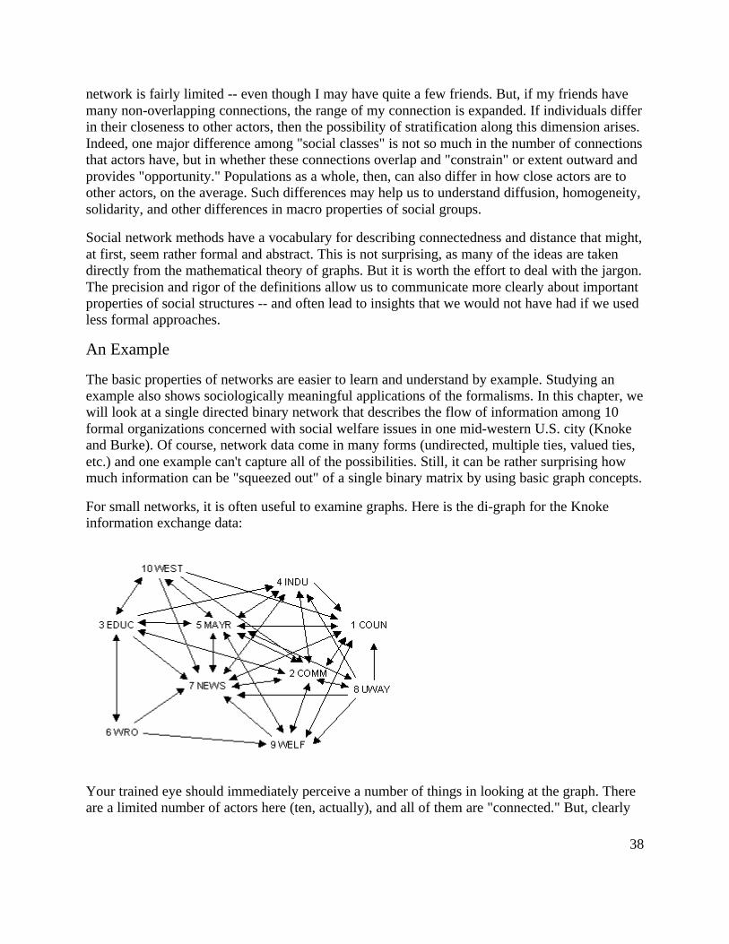
38

network is fairly limited -- even though I may have quite a few friends. But, if my friends havemany non-overlapping connections, the range of my connection is expanded. If individuals differin their closeness to other actors, then the possibility of stratification along this dimension arises.Indeed, one major difference among "social classes" is not so much in the number of connectionsthat actors have, but in whether these connections overlap and "constrain" or extent outward andprovides "opportunity." Populations as a whole, then, can also differ in how close actors are toother actors, on the average. Such differences may help us to understand diffusion, homogeneity,solidarity, and other differences in macro properties of social groups.

Social network methods have a vocabulary for describing connectedness and distance that might,at first, seem rather formal and abstract. This is not surprising, as many of the ideas are takendirectly from the mathematical theory of graphs. But it is worth the effort to deal with the jargon.The precision and rigor of the definitions allow us to communicate more clearly about importantproperties of social structures -- and often lead to insights that we would not have had if we usedless formal approaches.

An Example

The basic properties of networks are easier to learn and understand by example. Studying anexample also shows sociologically meaningful applications of the formalisms. In this chapter, wewill look at a single directed binary network that describes the flow of information among 10formal organizations concerned with social welfare issues in one mid-western U.S. city (Knokeand Burke). Of course, network data come in many forms (undirected, multiple ties, valued ties,etc.) and one example can't capture all of the possibilities. Still, it can be rather surprising howmuch information can be "squeezed out" of a single binary matrix by using basic graph concepts.

For small networks, it is often useful to examine graphs. Here is the di-graph for the Knokeinformation exchange data:

Your trained eye should immediately perceive a number of things in looking at the graph. Thereare a limited number of actors here (ten, actually), and all of them are "connected." But, clearly

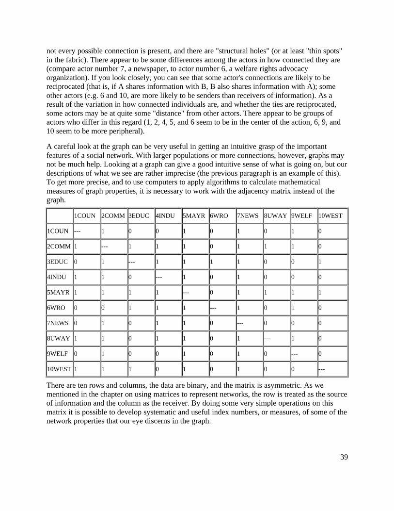
39

not every possible connection is present, and there are "structural holes" (or at least "thin spots"in the fabric). There appear to be some differences among the actors in how connected they are(compare actor number 7, a newspaper, to actor number 6, a welfare rights advocacyorganization). If you look closely, you can see that some actor's connections are likely to bereciprocated (that is, if A shares information with B, B also shares information with A); someother actors (e.g. 6 and 10, are more likely to be senders than receivers of information). As aresult of the variation in how connected individuals are, and whether the ties are reciprocated,some actors may be at quite some "distance" from other actors. There appear to be groups ofactors who differ in this regard (1, 2, 4, 5, and 6 seem to be in the center of the action, 6, 9, and10 seem to be more peripheral).

A careful look at the graph can be very useful in getting an intuitive grasp of the importantfeatures of a social network. With larger populations or more connections, however, graphs maynot be much help. Looking at a graph can give a good intuitive sense of what is going on, but ourdescriptions of what we see are rather imprecise (the previous paragraph is an example of this).To get more precise, and to use computers to apply algorithms to calculate mathematicalmeasures of graph properties, it is necessary to work with the adjacency matrix instead of thegraph.

1COUN 2COMM 3EDUC 4INDU 5MAYR 6WRO 7NEWS 8UWAY 9WELF 10WEST

1COUN --- 1 0 0 1 0 1 0 1 0

2COMM 1 --- 1 1 1 0 1 1 1 0

3EDUC 0 1 --- 1 1 1 1 0 0 1

4INDU 1 1 0 --- 1 0 1 0 0 0

5MAYR 1 1 1 1 --- 0 1 1 1 1

6WRO 0 0 1 1 1 --- 1 0 1 0

7NEWS 0 1 0 1 1 0 --- 0 0 0

8UWAY 1 1 0 1 1 0 1 --- 1 0

9WELF 0 1 0 0 1 0 1 0 --- 0

10WEST 1 1 1 0 1 0 1 0 0 ---

There are ten rows and columns, the data are binary, and the matrix is asymmetric. As wementioned in the chapter on using matrices to represent networks, the row is treated as the sourceof information and the column as the receiver. By doing some very simple operations on thismatrix it is possible to develop systematic and useful index numbers, or measures, of some of thenetwork properties that our eye discerns in the graph.

40

Connections

Since networks are defined by their actors and the connections among them, it is useful to beginour description of networks by examining these very simple properties. Focusing first on thenetwork as a whole, one might be interested in the number of actors, the number of connectionsthat are possible, and the number of connections that are actually present. Differences in the sizeof networks, and how connected the actors are tell us two things about human populations thatare critical. Small groups differ from large groups in many important ways -- indeed, populationsize is one of the most critical variables in all sociological analyses. Differences in howconnected the actors in a population are may be a key indicator of the solidarity, "moral density,"and "complexity" of the social organization of a population.

Individuals, as well as whole networks, differ in these basic demographic features. Individualactors may have many or few ties. Individuals may be "sources" of ties, "sinks" (actors thatreceive ties, but don't send them), or both. These kinds of very basic differences among actor'simmediate connections may be critical in explaining how they view the world, and how theworld views them. The number and kinds of ties that actors have are a basis for similarity ordissimilarity to other actors -- and hence to possible differention and stratification. The numberand kinds of ties that actors have are keys to determining how much their embeddedness in thenetwork constrains their behavior, and the range of opportunities, influence, and power that theyhave.

It is possible that a network is not completely connected. This is the question of reachability.There may be two or more disconnected groups in the population. If it is not possible for allactors to "reach" all other actors, then our population consists of more than one group. Thegroups may occupy the same space, or have the same name, but not all members are connected.Obviously, such divisions in populations may be sociologically significant. To the extent that anetwork is not connected, there may be a structural basis for stratification and conflict. At theindividual level, the degree to which an actor can reach others indicates the extent to which thatindividual is separated from the whole, or the extent to which that actor is isolated. Suchisolation may have social-psychological significance. If an actor cannot reach, or cannot bereached by another, then there can be no learning, support, or influence between the two.

Another useful way to look at networks as a whole, and the way in which individuals areembedded in them, is to examine the local structures. The most common approaches here hasbeen to look at dyads (i.e. sets of two actors) and triads (i.e. sets of three actors).

With directed data, there are four possible dyadic relationships: A and B are not connected, Asends to B, B sends to A, or A and B send to each other (with undirected data, there are only twopossible relationships - no tie or tie). It may be useful to look at each actor in terms of the kindsof dyadic relationships in which they are involved. An actor that sends, but does not receive tiesmay be quite different from one who both sends and receives. A common interest in looking atdyadic relationships is the extent to which ties are reciprocated. Some theorists feel that there isan equilibrium tendency toward dyadic relationships to be either null or reciprocated, and that

41

asymmetric ties may be unstable. Of course, one can examine the entire network, as well asindividual differences. In one sense, a network that has a predominance of null or reciprocatedties over asymmetric connections may be a more "equal" or "stable" network than one with apredominance of asymmetric connections (which might be more of a hierarchy).

Small group theorists argue that many of the most interesting and basic questions of socialstructure arise with regard to triads. Triads allow for a much wider range of possible sets ofrelations (with directed data, there are actually 64 possible types of relations among 3 actors!),including relationships that exhibit hierarchy, equality, and the formation of exclusive groups(e.g. where two actors connect, and exclude the third). Thus, small group researchers suggest, allof the really fundamental forms of social relationships can be observed in triads. Because of thisinterest, we may wish to conduct a "triad census" for each actor, and for the network as a whole.In particular, we may be interested in the proportion of triads that are "transitive" (that is, displaya type of balance where, if A directs a tie to B, and B directs a tie to C, then A also directs a tie toC). Such transitive or balanced triads are argued by some theorists to be the "equilibrium" ornatural state toward which triadic relationships tend (not all theorists would agree!).

So, there is really quite a lot that can be learned both about individual actors embeddedness, andabout the whole network structure just by examining the adjacencies. Let's turn to our data onorganizations in the social welfare field, and apply these ideas.

Size, density and degree

The size of a network is often a very important. Imagine a group of 12 students in a seminar. Itwould not be difficult for each of the students to know each of the others fairly well, and build upexchange relationships (e.g. sharing reading notes). Now imagine a large lecture class of 300students. It would be extremely difficult for any student to know all of the others, and it would bevirtually impossible for there to be a single network for exchanging reading notes. Size is criticalfor the structure of social relations because of the limited resources and capacities that each actorhas for building and maintaining ties. As a group gets bigger, the proportion of all of the ties thatcould (logically) be present -- density -- will fall, and the more likely it is that differentiated andpartitioned groups will emerge.

Our example network has ten actors. Usually the size of a network is indexed simply by countingthe number of nodes. In any network there are (k * k-1) unique ordered pairs of actors (that isAB is different from BA, and leaving aside self-ties), where k is the number of actors. You maywish to verify this for yourself with some small networks. So, in our network of 10 actors, withdirected data, there are 90 logically possible relationships. If we had undirected, or symmetricties, the number would be 45, since the relationship AB would be the same as BA. The numberof logically possible relationships then grows exponentially as the number of actors increaseslinearly. It follows from this that the range of logically possible social structures increases (or, byone definition, "complexity" increases) exponentially with size.

Fully saturated networks (i.e. one where all logically possible ties are actually present) areempirically rare, particularly where there are more than a few actors in the population. It is usefulto look at how close a network is to realizing this potential. That is, to examine the density of

42

ties, which is defined as the proportion of all ties that could be present that actually are. Here isthe relevant output from UCINET's univariate statistics routine.(For the whole Matrix)*********************

Mean 0.54 Std Dev 0.50 Sum 49 Variance 0.25 Minimum 0 Maximum 1 N of Obs 90

Notes: The mean is .54. That is, the mean strength of ties across all possible ties (ignoring self-ties) is .54. Since the data are binary, this means that 54% of all possible ties are present (i.e. thedensity of the matrix). The standard deviation is a measure of how much variation there is amongthe elements. If all elements were one, or all were zero, the standard deviation would be zero --no variation. Here, the average variability from one element to the next is .50, almost as large asthe mean. So, we would say that there is, relatively, a great deal of variation in ties. With binarydata, the maximum variability in ties -- or the maximum uncertainty about whether any given tieis likely to be present or absent -- is realized at a density of .50. As density approaches eitherzero or unity, the standard deviation and variance in ties will decline.

Since the data in our example are asymmetric (that is directed ties), we can distinguish betweenties being sent and ties being received. Looking at the density for each row and for each columncan tell us a good bit about the way in which actors are embedded in the overall density. Here arethe "row-wise" univariate statistics for our example from UCINET:

(for the rows, or sending of ties)************************************* Mean Std D Sum Var ---- ---- ---- ---- 1 0.44 0.50 4.00 0.25 2 0.78 0.42 7.00 0.17 3 0.67 0.47 6.00 0.22 4 0.44 0.50 4.00 0.25 5 0.89 0.31 8.00 0.10 6 0.33 0.47 3.00 0.22 7 0.33 0.47 3.00 0.22 8 0.67 0.47 6.00 0.22 9 0.33 0.47 3.00 0.22 10 0.56 0.50 5.00 0.25

Notes: Statistics on the rows tell us about the role that each actor plays as a "source" of ties (in adirected graph). The sum of the connections from the actor to others (e.g. actor #1 sendsinformation to four others) is called the out-degree of the point (for symmetric data, of course,each node simply has degree, as we cannot distinguish in-degree from out-degree). The degree

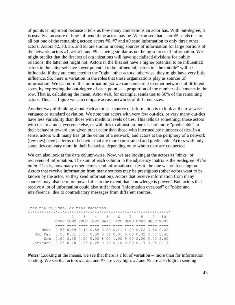
43

of points is important because it tells us how many connections an actor has. With out-degree, itis usually a measure of how influential the actor may be. We can see that actor #5 sends ties toall but one of the remaining actors; actors #6, #7 and #9 send information to only three otheractors. Actors #2, #3, #5, and #8 are similar in being sources of information for large portions ofthe network; actors #1, #6, #7, and #9 as being similar as not being sources of information. Wemight predict that the first set of organizations will have specialized divisions for publicrelations, the latter set might not. Actors in the first set have a higher potential to be influential;actors in the latter set have lower potential to be influential; actors in "the middle" will beinfluential if they are connected to the "right" other actors, otherwise, they might have very littleinfluence. So, there is variation in the roles that these organizations play as sources ofinformation. We can norm this information (so we can compare it to other networks of differentsizes, by expressing the out-degree of each point as a proportion of the number of elements in therow. That is, calculating the mean. Actor #10, for example, sends ties to 56% of the remainingactors. This is a figure we can compare across networks of different sizes.

Another way of thinking about each actor as a source of information is to look at the row-wisevariance or standard deviation. We note that actors with very few out-ties, or very many out-tieshave less variability than those with medium levels of ties. This tells us something: those actorswith ties to almost everyone else, or with ties to almost no-one else are more "predictable" intheir behavior toward any given other actor than those with intermediate numbers of ties. In asense, actors with many ties (at the center of a network) and actors at the periphery of a network(few ties) have patterns of behavior that are more constrained and predictable. Actors with onlysome ties can vary more in their behavior, depending on to whom they are connected.

We can also look at the data column-wise. Now, we are looking at the actors as "sinks" orrecievers of information. The sum of each column in the adjacency matrix is the in-degree of thepoint. That is, how many other actors send information or ties to the one we are focusing on.Actors that receive information from many sources may be prestigious (other actors want to beknown by the actor, so they send information). Actors that receive information from manysources may also be more powerful -- to the extent that "knowledge is power." But, actors thatreceive a lot of information could also suffer from "information overload" or "noise andinterference" due to contradictory messages from different sources.

(for the columns, or ties received)************************************************************** 1 2 3 4 5 6 7 8 9 10 COUN COMM EDUC INDU MAYR WRO NEWS UWAY WELF WEST ---- ---- ---- ---- ---- ---- ---- ---- ---- ---- Mean 0.56 0.89 0.44 0.56 0.89 0.11 1.00 0.22 0.56 0.22 Std Dev 0.50 0.31 0.50 0.50 0.31 0.31 0.00 0.42 0.50 0.42 Sum 5.00 8.00 4.00 5.00 8.00 1.00 9.00 2.00 5.00 2.00 Variance 0.25 0.10 0.25 0.25 0.10 0.10 0.00 0.17 0.25 0.17

Notes: Looking at the means, we see that there is a lot of variation -- more than for informationsending. We see that actors #2, #5, and #7 are very high. #2 and #5 are also high in sending

44

information -- so perhaps they act as "communicators" and "facilitators" in the system. Actor #7receives a lot of information, but does not send a lot. Actor #7, as it turns out is an "informationsink" -- it collects facts, but it does not create them (at least we hope so, since actor #7 is anewspaper). Actors #6, #8, and #10 appear to be "out of the loop" -- that is, they do not receiveinformation from many sources directly. Actor #6 also does not send much information -- so #6appears to be something of an "isolate." Numbers #8 and #10 send relatively more informationthan they receive. One might suggest that they are "outsiders" who are attempting to beinfluential, but may be "clueless."

We can learn a great deal about a network overall, and about the structural constraints onindividual actors, and even start forming some hypotheses about social roles and behavioraltendencies, just by looking at the simple adjacencies and calculating a few very basic statistics.Before discussing the slightly more complex idea of distance, there are a couple other aspects of"connectedness" that are sometimes of interest.

Reachability

An actor is "reachable" by another if there exists any set of connections by which we can tracefrom the source to the target actor, regardless of how many others fall between them. If the dataare asymmetric or directed, it is possible that actor A can reach actor B, but that actor B cannotreach actor A. With symmetric or undirected data, of course, each pair of actors either are or arenot reachable to one another. If some actors in a network cannot reach others, there is thepotential of a division of the network. Or, it may indicate that the population we are studying isreally composed of more than one separate sub-population.

In the Knoke information exchange data set, it turns out that all actors are reachable by all others.This is something that you can verify by eye. See if you can find any pair of actors in thediagram such that you cannot trace from the first to the second along arrows all headed in thesame direction (don't waste a lot of time on this, there is no such pair!).

45

Reciprocity and Transitivity

It might be useful, in some cases, to classify the dyadic relationships of each actor and for thenetwork as a whole. We've done this in the table below.

Node No ties In ties Out ties Reciprocated tiesNeighborhoodsize

1COUN 2 3 0 4 (58%) 7

2COMM 1 1 0 7 (88%) 8

3EDUC 3 0 2 4 (67%) 6

4INDU 3 2 1 3 (50%) 6

5MAYR 1 0 0 8 (100%) 8

6WRO 6 0 2 1 (33%) 3

7NEWS 0 5 0 4 (44%) 9

8UWAY 3 0 4 2 (33%) 6

9WELF 3 2 1 3 (50%) 6

10WEST 4 0 3 2 (40%) 5

Whole Network 39 13 13 38 (75%) 51

The neighborhood size for each actor is the number of other actors to whom they are adjacent.When we array the data about actor's adjacencies as we have here, there is a tendency tocharacterize actors in terms of the similarity of their tie profiles (much more on this, later). Someactors are predominantly "sources" (that is, they have a tendency to send more than to receive --actors #3, #6, and #8). Some actors may be predominantly "sinks" (that is, they have a tendencyto receive more than send -- actors #1, #5). Other actors may be "transmitters" that both send andreceive, but to different others. Perhaps most interestingly, the actors differ quite markedly intheir involvement in mutual or reciprocated relationships. Actors #2 and #5 stand out particularlyas having predominantly "symmetric" or balanced relationships with other actors.

For the network as a whole, we note that a very considerable proportion of the relationships arereciprocated. Such a structure is one in which a good deal of unmediated pair-wise

46

communication can occur. This might suggest a rather non-hierarchical structuring of theorganizational field, and a field in which there are many local and particular pair-wiserelationships, rather than a single monolithic structure or "establishment."

It is also useful to examine the connections in terms of triadic relations. The number of triads thatexist with 10 actors is very large; and, with directed data, each of the triads could be classifiedinto one of 64 types. Most commonly, interest has focused on transitive triads. The transitivityprinciple holds that, if A is tied to B, and B is tied to C, then A should be tied to C. The idea, like"balance" and "reciprocity" is that triadic relationships (where there are ties among the actors)should tend toward transitivity as an equilibrium condition. A special form of this notion is whatis called "balance theory." Balance theory deals specifically with relationships of positive andnegative affect. It argues that if A likes B, and B likes C, then A should come to like C. Or, if Alikes B and B dislikes C, then A should come to dislike C.

For the Knoke information exchange network, UCINET reports that 20.3% of all of the triadsthat could be transitive (i.e. those triads with three or more ties that connect all actors) aretransitive. This is not a particularly high level, and suggests either that the theory of a tendencytoward transitivity in triads has not been well realized in these data (perhaps because the systemhas not been operating very long), or that the theory does not apply in this case (more likely).

Distance

The properties of the network that we have examined so far primarily deal with adjacencies -- thedirect connections from one actor to the next. But the way that people are embedded in networksis more complex than this. Two persons, call them A and B, might each have five friends. Butsuppose that none of person A's friends have any friends except A. Person B's five friends, incontrast, each have five friends. The information available to B, and B's potential for influence isfar greater than A's. That is, sometimes being a "friend of a friend" may be quite consequential.

To capture this aspect of how individuals are embedded in networks, one main approach is toexamine the distance that an actor is from others. If two actors are adjacent, the distance betweenthem is one (that is, it takes one step for a signal to go from the source to the reciever). If A tellsB, and B tells C (and A does not tell C), then actors A and C are at a distance of two. How manyactors are at various distances from each actor can be important for understanding the differencesamong actors in the constraints and opportunities they have as a result of their position.Sometimes we are also interested in how many ways there are to connect between two actors, ata given distance. That is, can actor A reach actor B in more than one way? Sometimes multipleconnections may indicate a stronger connection between two actors than a single connection.

The distances among actors in a network may be an important macro-characteristic of thenetwork as a whole. Where distances are great, it may take a long time for information to diffuseacross a population. It may also be that some actors are quite unaware of, and influenced byothers -- even if they are technically reachable, the costs may be too high to conduct exchanges.The variability across the actors in the distances that they have from other actors may be a basisfor differentiation and even stratification. Those actors who are closer to more others may beable to exert more power than those who are more distant. We will have a good deal more to say

47

about this aspect of variability in actor distances in the next chapter.

For the moment, we need to learn a bit of jargon that is used to describe the distances betweenactors: walks, paths, and semi-paths. Using these basic definitions, we can then develop somemore powerful ways of describing various aspects of the distances among actors in a network.

Walks etc.

To describe the distances between actors in a network with precision, we need someterminology. And, as it turns out, whether we are talking about a simple graph or a directedgraph makes a good bit of difference. If A and B are adjacent in a simple graph, they have adistance of one. In a directed graph, however, A can be adjacent to B while B is not adjacent toA -- the distance from A to B is one, but there is no distance from B to A. Because of thisdifference, we need slightly different terms to describe distances between actors in graphs anddigraphs.

Simple graphs: The most general form of connection between two actors in a graph is called awalk. A walk is a sequence of actors and relations that begins and ends with actors. A closedwalk is one where the beginning and end point of the walk are the same actor. Walks areunrestricted. A walk can involve the same actor or the same relation multiple times. A cycle is aspecially restricted walk that is often used in algorithms examining the neighborhoods (the pointsadjacent) of actors. A cycle is a closed walk of 3 or more actors, all of who are distinct, exceptfor the origin/destination actor. The length of a walk is simply the number of relations containedin it. For example, consider this graph:

There are many walks in a graph (actually, an infinite number if we are willing to include walksof any length -- though, usually, we restrict our attention to fairly small lengths). To illustratejust a few, begin at actor A and go to actor C. There is one walk of length 2 (A,B,C). There isone walk of length three (A,B,D,C). There are several walks of length 4 (A,B,E,D,C; A,B,D,B,C;A,B,E,B,C). Because these are unrestricted, the same actors and relations can be used more thanonce in a given walk. There are no cycles beginning and ending with A. There are somebeginning and ending with actor B (B,D,C,B; B,E,D,B; B,C,D,E,B).

It is usually more useful to restrict our notion of what constitutes a connection somewhat. Onepossibility is to restrict the count only walks that do not re-use relations. A trail between twoactors is any walk that includes a given relation no more than once (the same other actors,however, can be part of a trail multiple times. The length of a trail is the number of relations in it.

48

All trails are walks, but not all walks are trails. If the trail begins and ends with the same actor, itis called a closed trail. In our example above, there are a number of trails from A to C. Excludedare tracings like A,B,D,B,C (which is a walk, but is not a trail because the relation BD is usedmore than once.

Perhaps the most useful definition of a connection between two actors (or between an actor andthemself) is a path. A path is a walk in which each other actor and each other relation in thegraph may be used at most one time. The single exception to this is a closed path, which beginsand ends with the same actor. All paths are trails and walks, but all walks and all trails are notpaths. In our example, there are a limited number of paths connecting A and C: A,B,C; A,B,D,C;A,B,E,D,C.

Directed graphs: Walks, trails, and paths can also be defined for directed graphs. But there aretwo flavors of each, depending on whether we want to take direction into account or not . Semi-walks, semi-trails, and semi-paths are the same as for undirected data. In defining thesedistances, the directionality of connections is simply ignored (that is, arcs - or directed ties aretreated as though they were edges - undirected ties). As always, the length of these distances isthe number of relations in the walk, trail, or path. If we do want to pay attention to thedirectionality of the connections we can define walks, trails, and paths in the same way as before,but with the restriction that we may not "change direction" as we move across relations fromactor to actor. Consider a directed graph:

In this di-graph, there are a number of walks from A to C. However, there are no walks from C(or anywhere else) to A. Some of these walks from A to C are also trails (e.g. A,B,E,D,B,C).There are, however, only three paths from A to C. One path is length 2 (A,B,C); one is lengththree (A,B,D,C); one is length four (A,B,E,D,C).

The various kinds of connections (walks, trails, paths) provide us with a number of differentways of thinking about the distances between actors. The main reason that networkers areconcerned with these distances is that they provide a way of thinking about the strength of ties orrelations. Actors that are connected at short lengths or distances may have stronger connections;actors that are connected many times (for example, having many, rather than a single path) mayhave stronger ties. Their connection may also be less subject to disruption, and hence more stableand reliable.

Let's look briefly at the distances between pairs of actors in the Knoke data on directedinformation flows:

49

# of walks of length 1 1 1 2 3 4 5 6 7 8 9 0 - - - - - - - - - - 1 0 1 0 0 1 0 1 0 1 0 2 1 0 1 1 1 0 1 1 1 0 3 0 1 0 1 1 1 1 0 0 1 4 1 1 0 0 1 0 1 0 0 0 5 1 1 1 1 0 0 1 1 1 1 6 0 0 1 0 0 0 1 0 1 0 7 0 1 0 1 1 0 0 0 0 0 8 1 1 0 1 1 0 1 0 1 0 9 0 1 0 0 1 0 1 0 0 0 10 1 1 1 0 1 0 1 0 0 0

# of walks of length 2 1 1 2 3 4 5 6 7 8 9 0 - - - - - - - - - - 1 2 3 2 3 3 0 3 2 2 1 2 3 7 1 4 6 1 6 1 3 2 3 4 4 4 3 4 0 5 2 3 1 4 2 3 2 3 3 0 3 2 3 1 5 4 7 2 4 8 1 7 1 3 1 6 0 3 0 2 3 1 2 0 0 1 7 3 2 2 2 2 0 3 2 2 1 8 3 5 2 3 5 0 5 2 3 1 9 2 2 2 3 2 0 2 2 2 1 10 2 4 2 4 4 1 4 2 3 2

# of walks of length 3 1 2 3 4 5 6 7 8 9 10 -- -- -- -- -- -- -- -- -- -- 1 12 18 7 13 18 2 18 6 10 5 2 20 26 16 21 27 1 28 13 18 7 3 14 26 9 19 26 4 25 8 14 8 4 12 19 7 13 19 2 19 6 10 5 5 21 30 17 25 29 2 31 15 21 10 6 9 8 8 8 8 0 10 6 7 3 7 9 17 5 11 17 2 16 4 9 4 8 16 24 11 19 24 2 24 10 15 7 9 10 16 5 10 16 2 16 4 8 4 10 16 23 11 16 23 2 24 8 13 6

50

Total number of walks (lengths 1, 2, 3) 1 2 3 4 5 6 7 8 9 10 -- -- -- -- -- -- -- -- -- -- 1 14 21 9 16 21 2 21 8 12 6 2 23 33 17 25 33 2 34 14 21 9 3 18 30 13 22 30 4 30 10 17 9 4 14 22 9 16 22 2 22 8 13 6 5 25 37 19 29 37 3 38 16 24 11 6 9 11 8 10 11 1 12 6 7 4 7 12 19 7 13 19 2 19 6 11 5 8 19 29 13 22 29 2 29 12 18 8 9 12 18 7 13 18 2 18 6 10 5 10 18 27 13 20 27 3 28 10 16 8

The inventory of the total connections among actors is primarily useful for getting a sense ofhow "close" each pair is, and for getting a sense of how closely coupled the entire system is.Here, we can see that using only connections of two steps (e.g. "A friend of a friend"), there is agreat deal of connection in the graph overall; we also see that there are sharp differences amongactors in their degree of connectedness, and who they are connected to. These differences can beused to understand how information moves in the network, which actors are likely to beinfluential on one another, and a number of other important properties.

Diameter and Geodesic distance

One particular definition of the distance between actors in a network is used by most algorithmsto define more complex properties of individual's positions and the structure of the network as awhole. This quantity is the geodesic distance. For both directed and undirected data, the geodesicdistance is the number of relations in the shortest possible walk from one actor to another (or,from an actor to themself, if we care, which we usually do not).

The geodesic distance is widely used in network analysis. There may be many connectionsbetween two actors in a network. If we consider how the relation between two actors mayprovide each with opportunity and constraint, it may well be the case that not all of these tiesmatter. For example, suppose that I am trying to send a message to Sue. Since I know her e-mailaddress, I can send it directly (a path of length 1). I also know Donna, and I know that Donna hasSue's email address. I could send my message for Sue to Donna, and ask her to forward it. Thiswould be a path of length two. Confronted with this choice, I am likely to choose the geodesicpath (i.e. directly to Sue) because it is less trouble and faster, and because it does not depend onDonna. That is, the geodesic path (or paths, as there can be more than one) is often the "optimal"or most "efficient" connection between two actors. Many algorithms in network analysis assumethat actors will use the geodesic path when alternatives are available.

51

Using UCINET, we can easily locate the lengths of the geodesic paths in our directed data oninformation exchanges.

Geodesic distances for information exchanges 1 1 2 3 4 5 6 7 8 9 0 - - - - - - - - - - 1 0 1 2 2 1 3 1 2 1 2 2 1 0 1 1 1 2 1 1 1 2 3 2 1 0 1 1 1 1 2 2 1 4 1 1 2 0 1 3 1 2 2 2 5 1 1 1 1 0 2 1 1 1 1 6 3 2 1 2 2 0 1 3 1 2 7 2 1 2 1 1 3 0 2 2 2 8 1 1 2 1 1 3 1 0 1 2 9 2 1 2 2 1 3 1 2 0 2 10 1 1 1 2 1 2 1 2 2 0

Notes: Because the network is dense, the geodesic path distances are generally small. Thissuggests that information may travel pretty quickly in this network. Also note that there is ageodesic distance for each xy and yx pair -- that is, the graph is fully connected, and all actorsare "reachable" from all others (that is, there exists a path of some length from each actor to eachother actor). When a network is not fully connected, we cannot exactly define the geodesicdistances among all pairs. The standard approach in such cases is to treat the geodesic distancebetween unconnected actors as a length greater than that of any real distance in the data. For eachactor, we could calculate the mean and standard deviation of their geodesic distances to describetheir closeness to all other actors. For each actor, that actor's largest geodesic distance is calledthe eccentricity -- a measure of how far a actor is from the furthest other.

Because the current network is fully connected, a message that starts anywhere will eventuallyreach everyone. Although the computer has not calculated it, we might want to calculate themean (or median) geodesic distance and the standard deviation in geodesic distances for thematrix, and for each actor row-wise and column-wise. This would tell us how far each actor isfrom each other as a source of information for the other; and how far each actor is from eachother actor who may be trying to influence them. It also tells us which actors behavior (in thiscase, whether they've heard something or not) is most predictable and least predictable.

In looking at the whole network, we see that it is connected, and that the average geodesicdistance among actors is quite small. This suggests a system in which information is likely toreach everyone, and to do so fairly quickly. To get another notion of the size of a network, wemight think about it's diameter. The diameter of a network is the largest geodesic distance in the(connected) network. In the current case, no actor is more than three steps from any other -- avery "compact" network. The diameter of a network tells us how "big" it is, in one sense (that is,how many steps are necessary to get from one side of it to the other). The diameter is also a

52

useful quantity in that it can be used to set an upper bound on the lengths of connections that westudy. Many researchers limit their explorations of the connections among actors to involveconnections that are no longer than the diameter of the network.

Sometimes the redundancy of connection is an important feature of a network structure. If thereare many efficient paths connecting two actors, the odds are improved that a signal will get fromone to the other. One index of this is a count of the number of geodesic paths between each pairof actors. Of course, if two actors are adjacent, there can only be one such path. I've edited thedisplay below to include only those pairs where there is more than one geodesic path:

# Of Geodesic Paths in Information Exchanges 1 1 2 3 4 5 6 7 8 9 0 - - - - - - - - - - 1 - - 2 3 - 2 - 2 - - 2 - - - - - - - - - 2 3 4 - - - - - - 2 3 - 4 - - 2 - - 2 - 2 3 - 5 - - - - - - - - - - 6 9 3 - 2 3 - - 6 - - 7 3 - 2 - - 2 - 2 2 - 8 - - 2 - - 2 - - - - 9 2 - 2 3 - 2 - 2 - - 10 - - - 4 - - - 2 3 -

Notes: We see that most of the geodesic connections among these actors are not only shortdistance, but that there are very often multiple shortest paths from x to y. This suggests a couplethings: information flow is not likely to break down, because there are multiple paths; and, it willbe difficult for any individual to be a powerful "broker" in this structure because most actorshave alternative efficient ways of connection to other actors that can by-pass any given actor.

Flow, cohesion, and influence,

The use of geodesic paths to examine properties of the distances between individuals and for thewhole network often makes a great deal of sense. But, there may be other cases where thedistance between two actors, and the connectedness of the graph as a whole is best thought of asinvolving all connections -- not just the most efficient ones. If I start a rumor, for example, it willpass through a network by all pathways -- not just the most efficient ones. How much credenceanother person gives my rumor may depend on how many times they hear it form differentsources -- and not how soon they hear it. For uses of distance like this, we need to take intoaccount all of the connections among actors.

Several approaches have been developed for counting the amount of connection between pairs ofactors that take into account all connections between them. These measures have been used for anumber of different purposes, and these differences are reflected in the algorithms used tocalculate them. We will examine three such ideas.

53

Maximum flow: One notion of how totally connected two actors are (called maximum flow byUCINET) asks how many different actors in the neighborhood of a source lead to pathways to atarget. If I need to get a message to you, and there is only one other person to whom I can sendthis for retransmission, my connection is weak - even if the person I send it to may have manyways of reaching you. If, on the other hand, there are four people to whom I can send mymessage, each of whom has one or more ways of retransmitting my message to you, then myconnection is stronger. This "flow" approach suggests that the strength of my tie to you is nostronger than the weakest link in the chain of connections, where weakness means a lack ofalternatives. This approach to connection between actors is closely connected to the notion ofbetween-ness that we will examine in the next chapter. It is also logically close to the idea thatthe number of pathways, not their length may be important in connecting people. For ourdirected information flow data, the results of UCINET's count of maximum flow are shownbelow. You should verify for yourself that, for example, there are four "choke points" in flowsfrom actor 1 to actor 2, but five such points in the flow from actor 2 to actor 1.

MAXIMUM FLOW 1 1 2 3 4 5 6 7 8 9 0 COCOEDINMAWRNEUWWEWE - - - - - - - - - - 1 COUN 0 4 3 4 4 1 4 2 4 2 2 COMM 5 0 3 5 7 1 7 2 5 2 3 EDUC 5 6 0 5 6 1 6 2 5 2 4 INDU 4 4 3 0 4 1 4 2 4 2 5 MAYR 5 8 3 5 0 1 8 2 5 2 6 WRO 3 3 3 3 3 0 3 2 3 2 7 NEWS 3 3 3 3 3 1 0 2 3 2 8 UWAY 5 6 3 5 6 1 6 0 5 2 9 WELF 3 3 3 3 3 1 3 2 0 2 10 WEST 5 5 3 5 5 1 5 2 5 0

SINGLE-LINK HIERARCHICAL CLUSTERING

U C E I M N C W W W W O D N A E O E E R A U U D Y W M L S O Y N C U R S M F T

1Level 6 8 1 3 4 5 7 2 9 0----- - - - - - - - - - - 8 . . . . . XXXXX . . 5 . . XXXXXXXXXXXXX . 2 . XXXXXXXXXXXXXXXXX 1 XXXXXXXXXXXXXXXXXXX

notes: As with almost any other measure of the relations between pairs of actors, it maysometimes be useful to see if we can classify actors as being more or less similar to one another

54

in terms of the pattern of their relation with all the other actors. Cluster analysis is one usefultechnique for finding groups of actors who have similar relationships with other actors. We willhave much more to say on this topic in later chapters.

In the current example, we see that actors #2, 5, and 7 are relatively similar to one another interms of their maximum flow distances from other actors. A quick check of the graph revealswhy this is. These three actors have many different ways of reaching one another, and all otheractors in the network. In this regard, they are very different from actor 6, who can depend on (atmost) only three other actors to make a connection.

Hubbell and Katz cohesion: The maximum flow approach focuses on the vulnerability orredundancy of connection between pairs of actors - kind of a "strength of the weakest link"argument. As an alternative approach, we might want to consider the strength of all links asdefining the connection. If we are interested in how much two actors may influence one another,or share a sense of common position, the full range of their connections should probably beconsidered.

Even if we want to include all connections between two actors, it may not make a great deal ofsense (in most cases) to consider a path of length 10 as important as a path of length 1. TheHubbell and Katz approaches count the total connections between actors (ties for undirecteddata, both sending and receiving ties for directed data). Each connection, however, is given aweight, according to it's length. The greater the length, the weaker the connection. How muchweaker the connection becomes with increasing length depends on an "attenuation" factor. In ourexample, below, we have used an attenuation factor of .5. That is, an adjacency receives a weightof one, a walk of length two receives a weight of .5, a connection of length three receives aweight of .5 squared (.25) etc. The Hubbell and Katz approaches are very similar. Katz includesan identity matrix (a connection of each actor with themselves) as the strongest connection; theHubbell approach does not. As calculated by UCINET, both approaches "norm" the results torange from large negative distances (that is, the actors are very close relative to the other pairs, orhave high cohesion) to large positive numbers (that is, the actors have large distance relative toothers)

Method: HUBBELL

1 2 3 4 5 6 7 8 9 10 COUN COMM EDUC INDU MAYR WRO NEWS UWAY WELF WEST ------ ------ ------ ------ ------ ------ ------ ------ ------ ------1 COUN -0.67 -0.67 2.00 -0.33 -0.67 2.00 0.33 -1.33 -1.33 1.332 COMM -0.92 -0.17 1.50 -0.08 -0.67 1.50 0.08 -0.83 -1.08 0.833 EDUC 5.83 3.33 -11.00 0.17 3.33 -11.00 -2.17 6.67 8.17 -7.674 INDU -1.50 -1.00 3.00 0.50 -1.00 3.00 0.50 -2.00 -2.50 2.005 MAYR 1.25 0.50 -2.50 -0.25 1.00 -2.50 -0.75 1.50 1.75 -1.506 WRO 3.83 2.33 -8.00 0.17 2.33 -7.00 -1.17 4.67 6.17 -5.677 NEWS -1.17 -0.67 2.00 0.17 -0.67 2.00 0.83 -1.33 -1.83 1.338 UWAY -3.83 -2.33 7.00 -0.17 -2.33 7.00 1.17 -3.67 -5.17 4.679 WELF -0.83 -0.33 1.00 -0.17 -0.33 1.00 0.17 -0.67 -0.17 0.6710 WEST 4.33 2.33 -8.00 -0.33 2.33 -8.00 -1.67 4.67 5.67 -4.67

55

Method: KATZ 1 2 3 4 5 6 7 8 9 10 COUN COMM EDUC INDU MAYR WRO NEWS UWAY WELF WEST ------ ------ ------ ------ ------ ------ ------ ------ ------ ------1 COUN -1.67 -0.67 2.00 -0.33 -0.67 2.00 0.33 -1.33 -1.33 1.332 COMM -0.92 -1.17 1.50 -0.08 -0.67 1.50 0.08 -0.83 -1.08 0.833 EDUC 5.83 3.33 -12.00 0.17 3.33 -11.00 -2.17 6.67 8.17 -7.674 INDU -1.50 -1.00 3.00 -0.50 -1.00 3.00 0.50 -2.00 -2.50 2.005 MAYR 1.25 0.50 -2.50 -0.25 0.00 -2.50 -0.75 1.50 1.75 -1.506 WRO 3.83 2.33 -8.00 0.17 2.33 -8.00 -1.17 4.67 6.17 -5.677 NEWS -1.17 -0.67 2.00 0.17 -0.67 2.00 -0.17 -1.33 -1.83 1.338 UWAY -3.83 -2.33 7.00 -0.17 -2.33 7.00 1.17 -4.67 -5.17 4.679 WELF -0.83 -0.33 1.00 -0.17 -0.33 1.00 0.17 -0.67 -1.17 0.6710 WEST 4.33 2.33 -8.00 -0.33 2.33 -8.00 -1.67 4.67 5.67 -5.67

As with all measures of pairwise properties, one could analyze the data much further. We couldsee which individuals are similar to which others (that is, are there groups or strata defined by thesimilarity of their total connections to all others in the network?). Our interest might also focuson the whole network, where we might examine the degree of variance, and the shape of thedistribution of the dyad connections. For example, a network in with the total connections amongall pairs of actors might be expected to behave very differently than one where there are radicaldifferences among actors.

Taylor's Influence: The Hubbell and Katz approach may make most sense when applied tosymmetric data, because they pay no attention to the directions of connections (i.e. A's tiesdirected to B are just as important as B's ties to A in defining the distance or solidarity --closeness-- between them). If we are more specifically interested in the influence of A on B in adirected graph, the Taylor influence approach provides an interesting alternative.

The Taylor measure, like the others, uses all connections, and applies an attenuation factor.Rather than standardizing on the whole resulting matrix, however, a different approach isadopted. The column marginals for each actor are subtracted from the row marginals, and theresult is then normed (what did he say?!). Translated into English, we look at the balancebetween each actor's sending connections (row marginals) and their receiving connections(column marginals). Positive values then reflect a preponderance of sending over receiving to theother actor of the pair -- or a balance of influence between the two. Note that the newspaper (#7)shows as being a net influencer with respect to most other actors in the result below, while thewelfare rights organization (#6) has a negative balance of influence with most other actors.

56

Method: TAYLOR

1 2 3 4 5 6 7 8 9 10 COUN COMM EDUC INDU MAYR WRO NEWS UWAY WELF WEST ----- ----- ----- ----- ----- ----- ----- ----- ----- ----- 1 COUN 0.00 -0.02 0.23 -0.07 0.12 0.11 -0.09 -0.15 0.03 0.18 2 COMM 0.02 0.00 0.11 -0.06 0.07 0.05 -0.05 -0.09 0.05 0.09 3 EDUC -0.23 -0.11 0.00 0.17 -0.36 0.18 0.26 0.02 -0.44 -0.02 4 INDU 0.07 0.06 -0.17 0.00 0.05 -0.17 -0.02 0.11 0.14 -0.14 5 MAYR -0.12 -0.07 0.36 -0.05 0.00 0.30 0.01 -0.23 -0.13 0.23 6 WRO -0.11 -0.05 -0.18 0.17 -0.30 0.00 0.19 0.14 -0.32 -0.14 7 NEWS 0.09 0.05 -0.26 0.02 -0.01 -0.19 0.00 0.15 0.12 -0.18 8 UWAY 0.15 0.09 -0.02 -0.11 0.23 -0.14 -0.15 0.00 0.28 0.00 9 WELF -0.03 -0.05 0.44 -0.14 0.13 0.32 -0.12 -0.28 0.00 0.31 10 WEST -0.18 -0.09 0.02 0.14 -0.23 0.14 0.18 -0.00 -0.31 0.00

As with most other measures, the various approaches to the distance between actors and in thenetwork as a whole provide a menu of choices. No one definition to measuring distance will bethe "right" choice for a given purpose. Sometimes we don't really know, before hand, whatapproach might be best, and we may have to try and test several.

Summary of chapter 5

There is a great deal of information about both individuals and the population in a singleadjacency matrix. In this chapter you have learned a lot of terminology for describing theconnections and distances between actors, and for whole populations.

One focus in basic network analysis is on the immediate neighborhood of each actor: the dyadsand triads in which they are involved. The degree of an actor, and the in-degree and out-degree(if the data are directed) tell us about the extent to which an actor may be constrained by, orconstrain others. The extent to which an actor can reach others in the network may be useful indescribing an actor's opportunity structure. We have also seen that it is possible to describe"types" of actors who may form groups or strata on the basis of their places in opportunitystructures -- e.g. "isolates" "sources" etc.

Most of the time and effort of most social actors is spent in very local contexts -- interacting indyads and triads. In looking at the connections of actors, we have suggested that the degree of"reciprocity" and "balance" and "transitivity" in relations can be regarded as important indicatorsof the stability and institutionalization (that is, the extent to which relations are taken for grantedand are norm governed) of actor's positions in social networks.

The local connections of actors are important for understanding the social behavior of the wholepopulation, as well as for understanding each individual. The size of the network, it's density,whether all actors are reachable by all others (i.e. is the whole population connected, or are theremultiple components?), whether ties tend to be reciprocal or transitive, and all the otherproperties that we examined for individual connections are meaningful in describing the whole

57

population. Both the typical levels of characteristics (e.g. the mean degree of points), and theamount of diversity in characteristics (e.g. the variance in the degree of points) may be importantin explaining macro behavior. Populations with high density respond differently to challengesfrom the environment than those with low density; populations with greater diversity inindividual densities may be more likely to develop stable social differentiation and stratification.

In this chapter we also examined some properties of individual's embeddedness and of wholenetworks that look at the broader, rather than the local neighborhoods of actors. A set ofspecialized terminology was introduced to describe the distances between pairs of actors: walks,trails, and paths. We noted that there are some important differences between un-directed anddirected data in applying these ideas of distance.

One of the most common and important approaches to indexing the distances between actors isthe geodesic. The geodesic is useful for describing the minimum distance between actors. Thegeodesic distances between pairs of actors are the most commonly used measure of closeness.The average geodesic distance for an actor to all others, the variation in these distances, and thenumber of geodesic distances to other actors may all describe important similarities anddifferences between actors in how and how closely they are connected to their entire population.

The geodesic distance, however, examines only a single connection between a pair of actors (or,in some cases several, if there are multiple geodesics connecting them). Sometimes the sum ofall connections between actors, rather than the shortest connection may be relevant. We haveexamined approaches to measuring the vulnerability of the connection between actors (flow), thepairwise solidarity of actors (Hubbell and Katz), and the potential influence of actors on others(Taylor). Again, it important to remember that differences and similarities among individualpersons in these aspects of their distances from others may form a structural basis fordifferentiation and stratification. And, as always, these more complex patterns of distances ofindividuals from all others are also a characteristic of the whole population -- as well asdescribing the constraints and opportunities facing individuals. For example, a population inwhich most actors have multiple geodesic distances to others will, most likely, behave quitedifferently from one in which there is little redundancy of efficient communication linkages(think about some different kinds of bureaucratic organizations -- say a medical clinic versus anautomobile factory).

We have seen that there is a great deal of information available in fairly simple examinations ofan adjacency matrix. Life, of course, can get more complicated. We could have multiple layers,or multiplex data; we could have data that gave information on the strength of ties, rather thansimple presence or absence. Nonetheless, the methods that we've used here will usually give youa pretty good grasp of what is going on in more complicated data.

Now that you have a pretty good grasp of the basics of connection and distance, you are ready touse these ideas to build some concepts and methods for describing somewhat more complicatedaspects of the network structures of populations. We will turn to two of the most important ofthese in the next chapters. We will first (chapter 6) examine the concept of centrality andcentralization, which are important to understanding power, stratification, ranking, and inequalityin social structures. Then, in chapter 7, we will turn our attention to examining sub structures

58

(larger than dyads and triads). Populations of social structures are almost always divided anddifferentiated into cliques, factions, and groups (which may, or may not be ranked). Building onthese ideas, we will conclude our introductory survey of network concepts (chapters 8-11) withattention to the more abstract, but theoretically important task of describing network positionsand social roles that are central concepts in sociological analysis.

Review questions for chapter 5

1. Explain the differences among the "three levels of analysis" of graphs (individual, aggregate,whole).

2. How is the size of a network measured? Why is population size so important is sociologicalanalysis?

3. You have a network of 5 actors, assuming no self-ties, what is the potential number of directedties? What is the potential number of un-directed ties?

4. How is density measured? Why is density important is sociological analysis?

5. What is the "degree of a point?" Why might it be important, sociologically, if some actorshave high degree and other actors have lower degree? What is the difference between "in-degree" and "out-degree?"

6. If actor "A" is reachable from actor "B" does that necessarily mean that actor "B" is reachablefrom actor "A?" Why or why not?

7. For pairs of actors with directed relations, there are four possible configurations of ties. Canyou show these? Which configurations are "balanced?" For a triad with undirected relations, howmany possible configurations of ties are there? Which ones are balanced or transitive?

8. What are the differences among walks, trails, and paths? Why are "paths" the most commonlyused approach to inter-actor distances in sociological analysis?

9. What is the "geodesic" distance between two actors? Many social network measures assumethat the geodesic path is the most important path between actors -- why is this a plausibleassumption?

10. I have two populations of ten actors each, one has a network diameter of 3, and the other hasa network diameter of 6. Can you explain this statement to someone who doesn't know socialnetwork analysis? Can you explain why this difference in diameter might be important inunderstanding differences between the two populations?

11. How do "weighted flow" approaches to social distance differ from "geodesic" approaches tosocial distance?

12. Why might it matter if two actors have more than one geodesic or other path between them?

Application questions for chapter 5

59

1. Think of the readings from the first part of the course. Which studies used the ideas ofconnectedness and density? Which studies used the ideas of distance? What specific approachesdid they use to measure these concepts?

2. Draw the graphs of a "star" a "circle" a "line" and a "hierarchy." Describe the size, potential,and density of each graph. Examine the degrees of points in each graph -- are there differencesamong actors? Do these differences tell us something about the "social roles" of the actors?Create a matrix for each graph that shows the geodesic distances between each pair of actors.Are there differences between the graphs in whether actors are connected by multiple geodesicdistances?

3. Think about a small group of people that you know well (maybe your family, neighbors, astudy group, etc.). Who helps whom in this group? What is the density of the ties? Are tiesreciprocated? Are triads transitive?

4. Chrysler Corporation has called on you to be a consultant. Their research division is taking toolong to generate new models of cars, and often the work of the "stylists" doesn't fit well with thework of the "manufacturing engineers" (the people who figure out how to actually build the car).Chrysler's research division is organized as a classical hierarchical bureaucracy with twobranches (stylists, manufacturing) coordinated through group managers and a division manager.Analyze the reasons why performance is poor. Suggest some alternative ways of organizing thatmight improve performance, and explain why they will help.

60

6. Centrality and Power

Introduction: Centrality and Power

All sociologists would agree that power is a fundamental property of social structures. There ismuch less agreement about what power is, and how we can describe and analyze it's causes andconsequences. In this chapter we will look at some of the main approaches that social networkanalysis has developed to study power, and the closely related concept of centrality.

Network thinking has contributed a number of important insights about social power. Perhapsmost importantly, the network approach emphasizes that power is inherently relational. Anindividual does not have power in the abstract, they have power because they can dominateothers -- ego's power is alter's dependence, and vice versa. Because power is a consequence ofpatterns of relations, the amount of power in social structures can vary. If a system is veryloosely coupled (low density) not much power can be exerted; in high-density systems there isthe potential for greater power. Power is both a systemic (macro) and relational (micro) property.The amount of power in a system and its distribution across actors are related, but are not thesame thing. Two systems can have the same amount of power, but it can be equally distributed inone and unequally distributed in another. Power in social networks may be viewed either as amicro property (i.e. it describes relations between actors) or as a macro property (i.e. one thatdescribes the entire population); as with other key sociological concepts, the macro and microare closely connected in social network thinking.

Network analysts often describe the way that an actor is embedded in a relational network asimposing constraints on the actor and offering the actor opportunities. Actors that face fewerconstraints, and have more opportunities than others are in favorable structural positions. Havinga favored position means that an actor may extract better bargains in exchanges, and that theactor will be a focus for deference and attention from those in less favored positions. But what dowe mean by "having a favored position" and having "more opportunities" and "fewerconstraints?" There are no single correct and final answers to these difficult questions. But,network analysis has made important contributions in providing precise definitions and concretemeasures of several different approaches to the notion of the power that attaches to positions instructures of social relations.

The several faces of power

To understand the approaches that network analysis uses to study power, it is useful to first thinkabout some very simple systems. Consider these three networks, which are called the "star,""line," and "circle."

61

A moment's thought ought to suggest that actor A has a highly favored structural position in thestar network, if the network is describing a relationship such as resource exchange or resourcesharing. But, exactly why is it that actor A has a "better" position than all of the others in the starnetwork? What about the position of A in the line network? Is being at the end of the line anadvantage or a disadvantage? Are all of the actors in the circle network really in exactly the samestructural position? We need to think about why structural location can be advantageous ordisadvantageous to actors. Let's focus our attention on why actor A is so obviously at anadvantage in the star network.

Degree: First, actor A has more opportunities and alternatives than other actors. If actor D electsto not provide A with a resource, A has a number of other places to go to get it; however, if Delects to not exchange with A, then D will not be able to exchange at all. The more ties an actorhas then, the more power they (may) have. In the star network, Actor A has degree six, all otheractors have degree one. This logic underlies measures of centrality and power based on actordegree, which we will discuss below. Actors who have more ties have greater opportunitiesbecause they have choices. This autonomy makes them less dependent on any specific otheractor, and hence more powerful.

Now, consider the circle network in terms of degree. Each actor has exactly the same number ofalternative trading partners (or degree), so all positions are equally advantaged or disadvantaged.In the line network, matters are a bit more complex. The actors at the end of the line (A and G)are actually at a structural disadvantage, but all others are apparently equal (actually, it's notreally quite that simple). Generally, though, actors that are more central to the structure, in thesense of having higher degree or more connections, tend to have favored positions, and hencemore power.

62

Closeness: The second reason why actor A is more powerful than the other actors in the starnetwork is that actor A is closer to more actors than any other actor. Power can be exerted bydirect bargaining and exchange. But power also comes from acting as a "reference point" bywhich other actors judge themselves, and by being a center of attention who's views are heard bylarger numbers of actors. Actors who are able to reach other actors at shorter path lengths, orwho are more reachable by other actors at shorter path lengths have favored positions. Thisstructural advantage can be translated into power. In the star network, actor A is at a geodesicdistance of one from all other actors; each other actor is at a geodesic distance of two from allother actors (but A). This logic of structural advantage underlies approaches that emphasize thedistribution of closeness and distance as a source of power.

Now consider the circle network in terms of actor closeness. Each actor lies at different pathlengths from the other actors, but all actors have identical distributions of closeness, and againwould appear to be equal in terms of their structural positions. In the line network, the middleactor (D) is closer to all other actors than are the set C,E, the set B,F, and the set A,G. Again, theactors at the ends of the line, or at the periphery, are at a disadvantage.

Betweenness: The third reason that actor A is advantaged in the star network is because actor Alies between each other pairs of actors, and no other actors lie between A and other actors. If Awants to contact F, A may simply do so. If F wants to contact B, they must do so by way of A.This gives actor A the capacity to broker contacts among other actors -- to extract "servicecharges" and to isolate actors or prevent contacts. The third aspect of a structurally advantagedposition then is in being between other actors.

In the circle network, each actor lies between each other pair of actors. Actually, there are twopathways connecting each pair of actors, and each third actor lies on one, but not on the other ofthem. Again, all actors are equally advantaged or disadvantaged. In the line network, our endpoints (A,G) do not lie between any pairs, and have no brokering power. Actors closer to themiddle of the chain lie on more pathways among pairs, and are again in an advantaged position.

Each of these three ideas -- degree, closeness, and betweenness -- has been elaborated in anumber of ways. We will examine three such elaborations briefly here. The eigenvector ofgeodesics approach builds on the notion of closeness/distance. The flow approach (which is verysimilar to the flow approach discussed in the last chapter) modifies the idea of between-ness. TheBonacich power measure is an important and widely used generalization of degree-basedapproaches to power. In the previous chapter we discussed several approaches to distance thatspoke to the influence of points on one another (Hubbell, Katz, Taylor). These approaches,which we will not discuss again here, can also be seen as generalizations of the closeness logicthat measure the power of actors.

Network analysts are more likely to describe their approaches as descriptions of centrality thanof power. Each of the three approaches (degree, closeness, betweenness) describe the locationsof individuals in terms of how close they are to the "center" of the action in a network -- thoughthe definitions of what it means to be at the center differ. It is more correct to describe networkapproaches this way -- measures of centrality -- than as measures of power. But, as we havesuggested here, there are several reasons why central positions tend to be powerful positions.

63

Degree centrality

Actors who have more ties to other actors may be advantaged positions. Because they have manyties, they may have alternative ways to satisfy needs, and hence are less dependent on otherindividuals. Because they have many ties, they may have access to, and be able to call on moreof the resources of the network as a whole. Because they have many ties, they are often third-parties and deal makers in exchanges among others, and are able to benefit from this brokerage.So, a very simple, but often very effective measure of an actor's centrality and power potential istheir degree.

In undirected data, actors differ from one another only in how many connections they have. Withdirected data, however, it can be important to distinguish centrality based on in-degree fromcentrality based on out-degree. If an actor receives many ties, they are often said to beprominent, or to have high prestige. That is, many other actors seek to direct ties to them, andthis may indicate their importance. Actors who have unusually high out-degree are actors whoare able to exchange with many others, or make many others aware of their views. Actors whodisplay high out-degree centrality are often said to be influential actors.

Recall the data on information exchanges among organizations operating in the social welfarefield (Knoke) which we have been examining.

Let's examine the in-degrees and out-degrees of the points as a measure of who is "central" or"influential" in this network. UCINET has been used to do the counting, and some additionalcalculations and standardizations that were suggested by Linton Freeman.

64

FREEMAN'S DEGREE CENTRALITY MEASURES

1 2 3 4 OutDegree InDegree NrmOutDeg NrmInDeg ------------ ------------ ------------ ------------ 1 COUN 4.00 5.00 44.44 55.56 2 COMM 7.00 8.00 77.78 88.89 3 EDUC 6.00 4.00 66.67 44.44 4 INDU 4.00 5.00 44.44 55.56 5 MAYR 8.00 8.00 88.89 88.89 6 WRO 3.00 1.00 33.33 11.11 7 NEWS 3.00 9.00 33.33 100.00 8 UWAY 6.00 2.00 66.67 22.22 9 WELF 3.00 5.00 33.33 55.56 10 WEST 5.00 2.00 55.56 22.22

DESCRIPTIVE STATISTICS

1 2 3 4 OutDegree InDegree NrmOutDeg NrmInDeg ------------ ------------ ------------ ------------ Mean 4.90 4.90 54.44 54.44 Std Dev 1.70 2.62 18.89 29.17 Variance 2.89 6.89 356.79 850.62 Minimum 3.00 1.00 33.33 11.11 Maximum 8.00 9.00 88.89 100.00

Network Centralization (Outdegree) = 43.056%Network Centralization (Indegree) = 56.944%

notes: Actors #5 and #2 have the greatest out-degrees, and might be regarded as the mostinfluential (though it might matter to whom they are sending information, this measure does nottake that into account). Actors #5 and #2 are joined by #7 (the newspaper) when we examine in-degree. That other organizations share information with these three would seem to indicate adesire on the part of others to exert influence. This is an act of deference, or recognition that thepositions of actors 5, 2, and 7 might be worth trying to influence. If we were interested incomparing across networks of different sizes or densities, it might be useful to "standardize" themeasures of in and out-degree. In the last two columns of the first panel of results above, all thedegree counts have been expressed as percentages of the largest degree count in the data set (i.e.#7's out-degree of 9).

The next panel of results speaks to the "meso" level of analysis. That is, what does thedistribution of the actor's degree centrality scores look like? On the average, actors have a degreeof 4.9, which is quite high, given that there are only nine other actors. We see that the range ofin-degree is slightly larger (minimum and maximum) than that of out-degree, and that there ismore variability across the actors in in-degree than out-degree (standard deviations andvariances). The range and variability of degree (and other network properties) can be quite

65

important, because it describes whether the population is homogeneous or hetrogeneous instructural positions. One could examine whether the variability is high or low relative to thetypical scores by calculating the coefficient of variation (standard deviation divided by mean,times 100) for in-degree and out-degree. By the rules of thumb that are often used to evaluatecoefficients of variation, the current values (35 for out-degree and 53 for in-degree) aremoderate. Clearly, however, the population is more homogeneous with regard to out-degree(influence) than with regard to in-degree (prominence).

The last bit of information provided by the output above are Freeman's graph centralizationmeasures, which describe the population as a whole -- the macro level. These are very usefulstatistics, but require a bit of explanation.

Remember our "star" network from the discussion above (if not, go review it)? The star networkis the most centralized or most unequal possible network for any number of actors. In the starnetwork, all the actors but one have degree of one, and the "star" has degree of the number ofactors, less one. Freeman felt that it would be useful to express the degree of variability in thedegrees of actors in our observed network as a percentage of that in a star network of the samesize. This is how the Freeman graph centralization measures can be understood: they express thedegree of inequality or variance in our network as a percentage of that of a perfect star networkof the same size. In the current case, the out-degree graph centralization is 43% and the in-degreegraph centralization 57% of these theoretical maximums. We would arrive at the conclusion thatthere is a substantial amount of concentration or centralization in this whole network. That is, thepower of individual actors varies rather substantially, and this means that, overall, positionaladvantages are rather unequally distributed in this network.

Now that we understand the basic ideas, we can be a bit briefer in looking at the otherapproaches to centralization and power.

Closeness centrality

Degree centrality measures might be criticized because they only take into account theimmediate ties that an actor has, rather than indirect ties to all others. One actor might be tied toa large number of others, but those others might be rather disconnected from the network as awhole. In a case like this, the actor could be quite central, but only in a local neighborhood.

Closeness centrality approaches emphasize the distance of an actor to all others in the networkby focusing on the geodesic distance from each actor to all others. One could consider eitherdirected or undirected geodesic distances among actors. In our current example, we have decidedto look at undirected ties. The sum of these geodesic distances for each actor is the "farness" ofthe actor from all others. We can convert this into a measure of nearness or closeness centralityby taking the reciprocal (that is one divided by the farness) and norming it relative to the mostcentral actor. Here are the UCINET results for our information exchange data.

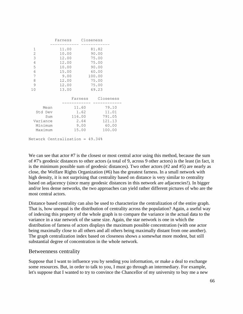
66

Farness Closeness ------------ ------------ 1 11.00 81.82 2 10.00 90.00 3 12.00 75.00 4 12.00 75.00 5 10.00 90.00 6 15.00 60.00 7 9.00 100.00 8 12.00 75.00 9 12.00 75.00 10 13.00 69.23

Farness Closeness ------------ ------------ Mean 11.60 79.10 Std Dev 1.62 11.01 Sum 116.00 791.05 Variance 2.64 121.13 Minimum 9.00 60.00 Maximum 15.00 100.00

Network Centralization = 49.34%

We can see that actor #7 is the closest or most central actor using this method, because the sumof #7's geodesic distances to other actors (a total of 9, across 9 other actors) is the least (in fact, itis the minimum possible sum of geodesic distances). Two other actors (#2 and #5) are nearly asclose, the Welfare Rights Organization (#6) has the greatest farness. In a small network withhigh density, it is not surprising that centrality based on distance is very similar to centralitybased on adjacency (since many geodesic distances in this network are adjacencies!). In biggerand/or less dense networks, the two approaches can yield rather different pictures of who are themost central actors.

Distance based centrality can also be used to characterize the centralization of the entire graph.That is, how unequal is the distribution of centrality across the population? Again, a useful wayof indexing this property of the whole graph is to compare the variance in the actual data to thevariance in a star network of the same size. Again, the star network is one in which thedistribution of farness of actors displays the maximum possible concentration (with one actorbeing maximally close to all others and all others being maximally distant from one another).The graph centralization index based on closeness shows a somewhat more modest, but stillsubstantial degree of concentration in the whole network.

Betweenness centrality

Suppose that I want to influence you by sending you information, or make a deal to exchangesome resources. But, in order to talk to you, I must go through an intermediary. For example,let's suppose that I wanted to try to convince the Chancellor of my university to buy me a new

67

computer. According to the rules of our bureaucratic hierarchy, I must forward my requestthrough my department chair, a dean, and an executive vice chancellor. Each one of these peoplecould delay the request, or even prevent my request from getting through. This gives the peoplewho lie "between" me and the Chancellor power with respect to me. To stretch the example justa bit more, suppose that I also have an appointment in the school of business, as well as one inthe department of sociology. I might forward my request to the Chancellor by both channels.Having more than one channel makes me less dependent, and, in a sense, more powerful.

Betweenness centrality views an actor as being in a favored position to the extent that the actorfalls on the geodesic paths between other pairs of actors in the network. That is, the more peopledepend on me to make connections with other people, the more power I have. If, however, twoactors are connected by more than one geodesic path, and I am not on all of them, I lose somepower. Using the computer, it is quite easy to locate the geodesic paths between all pairs ofactors, and to count up how frequently each actor falls in each of these pathways. If we add up,for each actor, the proportion of times that they are "between" other actors for the sending ofinformation in the Knoke data, we get the a measure of actor centrality. We can norm thismeasure by expressing it as a percentage of the maximum possible betweenness that an actorcould have had. The results from UCINET are:

Normed Between Between ------------ ------------ 1 0.67 0.93 2 12.33 17.13 3 11.69 16.24 4 0.81 1.12 5 17.83 24.77 6 0.33 0.46 7 2.75 3.82 8 0.00 0.00 9 1.22 1.70 10 0.36 0.50

Between nBetween ------------ ------------ Mean 4.80 6.67 Std Dev 6.22 8.64 Sum 48.00 66.67 Variance 38.69 74.63 Minimum 0.00 0.00 Maximum 17.83 24.77

Network Centralization Index = 20.11%

Notes: We can see that there is a lot of variation in actor between-ness (from zero to 17.83), andthat there is quite a bit of variation (std. dev. = 6.2 relative to a mean between-ness of 4.8).Despite this, the overall network centralization is relatively low. This makes sense, because we

68

know that fully one half of all connections can be made in this network without the aid of anyintermediary -- hence there cannot be a lot of "between-ness." In the sense of structuralconstraint, there is not a lot of "power" in this network. Actors #2, #3, and #5 appear to berelatively a good bit more powerful than others are by this measure. Clearly, there is a structuralbasis for these actors to perceive that they are "different" from others in the population. Indeed, itwould not be surprising if these three actors saw themselves as the movers-and-shakers, and thedealmakers that made things happen. In this sense, even though there is not very muchbetweenness power in the system, it could be important for group formation and stratification.

Each of the three basic approaches to centrality and power (degree, closeness, and betweenness)can, and has been elaborated to capture additional information from graphs. Reviewing a few ofthese elaborations may suggest some other ways in which power and position in networks arerelated.

Eigenvector of the geodesic distances

The closeness centrality measure described above is based on the sum of the geodesic distancesfrom each actor to all others (farness). In larger and more complex networks than the examplewe've been considering, it is possible to be somewhat misled by this measure. Consider twoactors, A and B. Actor A is quite close to a small and fairly closed group within a larger network,and rather distant from many of the members of the population. Actor B is at a moderate distancefrom all of the members of the population. The farness measures for actor A and actor B couldbe quite similar in magnitude. In a sense, however, actor B is really more "central" than actor Ain this example, because B is able to reach more of the network with same amount of effort.

The eigenvector approach is an effort to find the most central actors (i.e. those with the smallestfarness from others) in terms of the "global" or "overall" structure of the network, and to pay lessattention to patterns that are more "local." The method used to do this (factor analysis) is beyondthe scope of the current text. In a general way, what factor analysis does is to identify"dimensions" of the distances among actors. The location of each actor with respect to eachdimension is called an "eigenvalue," and the collection of such values is called the "eigenvector."Usually, the first dimension captures the "global" aspects of distances among actors; second andfurther dimensions capture more specific and local sub-structures.

For illustration, we have used UCINET to calculate the eigenvectors of the distance matrix forthe Knoke information exchange data. In this example, we have measured the distance betweentwo actors as the longer of the directed geodesic distances between them. If we were interested ininformation "exchange" relationships, rather than simply sources or receivers of information, wemight want to take this approach -- because it says that, in order to be close, a pair of actors musthave short distances between themselves in both directions. Here's the output:

69

BONACICH CENTRALITY

WARNING: This version of the program cannot handle asymmetric data. Matrix symmetrized by taking larger of Xij and Xji.

EIGENVALUES

FACTOR VALUE PERCENT CUM % RATIO ------- ------ ------- ------- ------- 1: 6.766 74.3 74.3 5.595 2: 1.209 13.3 87.6 1.282 3: 0.944 10.4 97.9 5.037 4: 0.187 2.1 100.0 ======= ====== ======= ======= ======= 9.106 100.0

Bonacich Eigenvector Centralities 1 2 Eigenvec nEigenvec --------- --------- 1 COUN 0.343 48.516 2 COMM 0.379 53.538 3 EDUC 0.276 38.999 4 INDU 0.308 43.522 5 MAYR 0.379 53.538 6 WRO 0.142 20.079 7 NEWS 0.397 56.124 8 UWAY 0.309 43.744 9 WELF 0.288 40.726 10 WEST 0.262 37.057

Descriptive Statistics

1 2 EigenvenEigenv ------ ------ 1 Mean 0.31 43.58 2 Std Dev 0.07 10.02 3 Sum 3.08 435.84 4 Variance 0.01 100.41 5 Euc Norm 1.00 141.42 6 Minimum 0.14 20.08 7 Maximum 0.40 56.12 8 N of Obs 10.00 10.00

Network centralization index = 20.90%

The first set of statistics, the eigenvalues, tell us how much of the overall pattern of distancesamong actors can be seen as reflecting the global pattern (the first eigenvalue), and more local, oradditional patterns (the additional patterns). We are interested in the percentage of the overall

70

variation in distances that is accounted for by the first factor. Here, this percentage is 74.3%.This means that about 3/4 of all of the distances among actors are reflective of the maindimension or pattern. If this amount is not large (say over 70%), great caution should beexercised in interpreting the further results, because the dominant pattern is not doing a verycomplete job of describing the data. The first eigenvalue should also be considerably larger thanthe second (here, the ratio of the first eigenvalue to the second is about 5.6 to 1). This means thatthe dominant pattern is, in a sense, 5.6 times as "important" as the secondary pattern.

Next, we turn our attention to the scores of each of the cases on the 1st eigenvector. Higherscores indicate that actors are "more central" to the main pattern of distances among all of theactors, lower values indicate that actors are more peripheral. The results are very similar to thosefor our earlier analysis of closeness centrality, with actors #7, #5, and #2 being most central, andactor #6 being most peripheral. Usually the eigenvalue approach will do what it is supposed todo: give us a "cleaned-up" version of the closeness centrality measures, as it does here. It is agood idea to examine both, and to compare them.

Last, we examine the overall centralization of the graph, and the distribution of centralities.There is relatively little variability in centralities (standard deviation .07) around the mean (.31).This suggests that, overall, there are not great inequalities in actor centrality or power, whenmeasured in this way. Compared to the pure "star" network, the degree of inequality orconcentration of the Knoke data is only 20.9% of the maximum possible. This is much less thanthe network centralization measure for the "raw" closeness measure (49.3), and suggests thatsome of the apparent differences in power using the raw closeness approach may be due more tolocal than to global inequalities.

The factor analysis approach could be used to examine degree or betweenness as well, but wewill not burden you with these exercises. Our main point is this: geodesic distances among actorsare a reasonable measure of one aspect of centrality -- or positional advantage. Sometimes theseadvantages may be more local, and sometimes more global. The factor-analytic approach is oneapproach that may sometimes help us to focus on the more global pattern. Again, it is not thatone approach is "right" and the other "wrong." Depending on the goals of our analysis, we maywish to emphasize one or the other aspects of the positional advantages that arise from centrality.

Flow centrality

The betweenness centrality measure we examined above characterizes actors as havingpositional advantage, or power, to the extent that they fall on the shortest (geodesic) pathwaybetween other pairs of actors. The idea is that actors who are "between" other actors, and onwhom other actors must depend to conduct exchanges, will be able to translate this broker roleinto power.

Suppose that two actors want to have a relationship, but the geodesic path between them isblocked by a reluctant broker. If there exists another pathway, the two actors are likely to use it,even if it is longer and "less efficient." In general, actors may use all of the pathways connectingthem, rather than just geodesic paths. The flow approach to centrality expands the notion ofbetweenness centrality. It assumes that actors will use all pathways that connect them,

71

proportionally to the length of the pathways. Betweenness is measured by the proportion of theentire flow between two actors (that is, through all of the pathways connecting them) that occurson paths of which a given actor is a part. For each actor, then, the measure adds up how involvedthat actor is in all of the flows between all other pairs of actors (the amount of computation withmore than a couple actors can be pretty intimidating!). Since the magnitude of this index numberwould be expected to increase with sheer size of the network and with network density, it isuseful to standardize it by calculating the flow betweenness of each actor in ratio to the total flowbetweeness that does not involve the actor.

FLOW BETWEENNESS CENTRALITY

FlowBet nFlowBet ------------ ------------ 1 10.00 7.69 2 49.00 39.20 3 17.00 12.50 4 14.00 10.53 5 48.00 37.80 6 2.00 1.34 7 23.00 16.67 8 8.00 6.06 9 9.00 6.34 10 12.00 9.09

DESCRIPTIVE STATISTICS FOR EACH MEASURE

FlowBet nFlowBet ------------ ------------ Mean 19.20 14.72 Std Dev 15.57 12.50 Sum 192.00 147.21 Variance 242.56 156.33 Minimum 2.00 1.34 Maximum 49.00 39.20

Network Centralization Index = 27.199

By this more complete measure of betweenness centrality, actors #2 and #5 are clearly the mostimportant mediators (with the newspaper, #7, being a distant third). Actor #3, who was fairlyimportant when we considered only geodesic flows, appears to be rather less important. Whilethe overall picture does not change a great deal, the elaborated definition of betweenness doesgive us a somewhat different impression of who is most central in this network.

Some actors are clearly more central than others, and the relative variability in flow betweennessof the actors is fairly great (the standard deviation of normed flow betweenness is 14.7 relative toa mean of 12.5, giving a coefficient of relative variation of 85%). Despite this relatively highamount of variation, the degree of inequality, or concentration in the distribution of flowbetweenness centralities among the actors is fairly low -- relative to that of a pure star network

72

(the network centralization index is 27.199). This is slightly higher than the index for thebetweenness measure that was based only on geodesic distances.

The Bonacich power index

Phillip Bonacich proposed a modification of the degree centrality approach that has been widelyaccepted as superior to the original measure. Bonacich's idea, like most good ones, is prettysimple. The original degree centrality approach argues that actors who have more connectionsare more likely to be powerful because they can directly affect more other actors. This makessense, but having the same degree does not necessarily make actors equally important.

Suppose that Bill and Fred each have five close friends. Bill's friends, however, happen to bepretty isolated folks, and don't have many other friends, save Bill. Fred's friends each also havelots of friends, who have lots of friends, and so on. Who is more central? We would probablyagree that Fred is, because the people he is connected to are better connected than Bill's people.Bonacich argued that one's centrality is a function of how many connections one has, and howmany the connections the actors in the neighborhood had.

While we have argued that more central actors are more likely to be more powerful actors,Bonacich questioned this idea. Compare Bill and Fred again. Fred is clearly more central, but ishe more powerful? One argument would be that one is likely to be more influential if one isconnected to central others -- because one can quickly reach a lot of other actors with one'smessage. But if the actors that you are connected to are, themselves, well connected, they are nothighly dependent on you -- they have many contacts, just as you do. If, on the other hand, thepeople to whom you are connected are not, themselves, well connected, then they are dependenton you. Bonacich argued that being connected to connected others makes an actor central, butnot powerful. Somewhat ironically, being connected to others that are not well connected makesone powerful, because these other actors are dependent on you -- whereas well connected actorsare not.

Bonacich proposed that both centrality and power were a function of the connections of theactors in one's neighborhood. The more connections the actors in your neighborhood have, themore central you are. The fewer the connections the actors in your neighborhood, the morepowerful you are. There would seem to be a problem with building an algorithm to capture theseideas. Suppose A and B are connected. Actor A's power and centrality are functions of her ownconnections, and also the connections of actor B. Similarly, actor B's power and centralitydepend on actor A's. So, each actor's power and centrality depends on each other actor's powersimultaneously.

There is a way out of this chicken-and-egg type of problem. Bonacich showed that, forsymmetric systems, an iterative estimation approach to solving this simultaneous equationsproblem would eventually converge to a single answer. One begins by giving each actor anestimated centrality equal to their own degree, plus a weighted function of the degrees of theactors to whom they were connected. Then, we do this again, using the first estimates (i.e. weagain give each actor an estimated centrality equal to their own first score plus the first scores ofthose to whom they are connected). As we do this numerous times, the relative sizes (not the

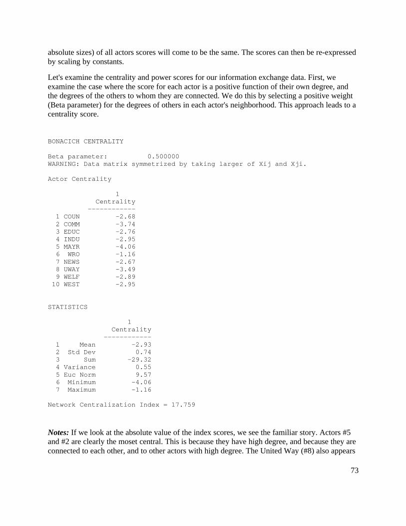
73

absolute sizes) of all actors scores will come to be the same. The scores can then be re-expressedby scaling by constants.

Let's examine the centrality and power scores for our information exchange data. First, weexamine the case where the score for each actor is a positive function of their own degree, andthe degrees of the others to whom they are connected. We do this by selecting a positive weight(Beta parameter) for the degrees of others in each actor's neighborhood. This approach leads to acentrality score.

BONACICH CENTRALITY

Beta parameter: 0.500000WARNING: Data matrix symmetrized by taking larger of Xij and Xji.

Actor Centrality

1 Centrality ------------ 1 COUN -2.68 2 COMM -3.74 3 EDUC -2.76 4 INDU -2.95 5 MAYR -4.06 6 WRO -1.16 7 NEWS -2.67 8 UWAY -3.49 9 WELF -2.89 10 WEST -2.95

STATISTICS

1 Centrality ------------ 1 Mean -2.93 2 Std Dev 0.74 3 Sum -29.32 4 Variance 0.55 5 Euc Norm 9.57 6 Minimum -4.06 7 Maximum -1.16

Network Centralization Index = 17.759

Notes: If we look at the absolute value of the index scores, we see the familiar story. Actors #5and #2 are clearly the moset central. This is because they have high degree, and because they areconnected to each other, and to other actors with high degree. The United Way (#8) also appears

74

to have high centrality by this measure -- this is a new result. In this case, it is because the UnitedWay is connected to all of the other high degree points by being a source to them -- and we havecounted being either a source or a sink as a link.

When we take into account the connections of those to whom each actor is connected, there isless variation in the data than when we examine only adjacencies. The standard deviation of theactor's centralities is fairly small relative to the mean score. This suggests relatively littledispersion or inequality in centralities, which is confirmed by comparing the distribution of thedata to that of a perfect star network (i.e. Network centralization index = 17.759).

Let's take a look at the power side of the index, which is calculated by the same algorithm, butgives negative weights to connections with well connected others, and positive weights forconnections to weakly connected others.

BONACICH POWERBeta parameter: -0.500000WARNING: Data matrix symmetrized by taking larger of Xij and Xji.

Actor Power

1 Power ------------ 1 COUN -1.00 2 COMM 2.00 3 EDUC 1.00 4 INDU 1.00 5 MAYR 3.00 6 WRO -0.00 7 NEWS 3.00 8 UWAY 1.00 9 WELF 2.00 10 WEST 1.00

STATISTICS 1 Power ------------ 1 Mean 1.30 2 Std Dev 1.19 3 Sum 13.00 4 Variance 1.41 5 Euc Norm 5.57 6 Minimum -1.00 7 Maximum 3.00

Network Centralization Index = 17.000

75

Notes: Not surprisingly, these results are rather different from many of the others we'veexamined. I say this is not surprising because most of the measures we've looked at equatecentrality with power, whereas the Bonacich power index views power as quite distinct fromcentrality.

The mayor (#5) and Comm (#2) are both central (from previous results) and powerful. Both ofthese actors are connected to almost everyone else -- including both the well connected and theweakly connected. Actor #9 (WELF) is identified by this index as being among the morepowerful actors. This is probably because of their tie to the WRO (#6) a weakly connected actor.Actor #1, which has high degree, is seen here as not being powerful. If you scan the diagramagain, you can see that actor #1's connections are almost all to other highly connected actors.

The Bonacich approach to degree-based centrality and degree-based power are fairly naturalextensions of the idea of degree centrality based on adjacencies. One is simply taking intoaccount the connections of one's connections, in addition to one's own connections. The notionthat power arises from connection to weak others, as opposed to strong others is an interestingone, and points to yet another way in which the positions of actors in network structures endowthem with different potentials.

Summary of chapter 6

Social network analysis methods provide some useful tools for addressing one of the mostimportant (but also one of the most complex and difficult), aspects of social structure: thesources and distribution of power. The network perspective suggests that the power of individualactors is not an individual attribute, but arises from their relations with others. Whole socialstructures may also be seen as displaying high levels or low levels of power as a result ofvariations in the patterns of ties among actors. And, the degree of inequality or concentration ofpower in a population may be indexed.

Power arises from occupying advantageous positions in networks of relations. Three basicsources of advantage are high degree, high closeness, and high betweenness. In simple structures(such as the star, circle, or line), these advantages tend to covary. In more complex and largernetworks, there can be considerable disjuncture between these characteristics of a position-- sothat an actor may be located in a position that is advantageous in some ways, anddisadvantageous in others.

We have reviewed three basic measures of "centrality" of individual positions, and someelaboration on each of the three main ideas of degree, closeness, and betweenness. This review isnot exhaustive. The question of how structural position confers power remains a topic of activeresearch and considerable debate. As you can see, different definitions and measures can capturedifferent ideas about where power comes from, and can result in some rather different insightsabout social structures.

In the last chapter and this one, we have emphasized that social network analysis methods giveus, at the same time, views of individuals and of whole populations. One of the most enduringand important themes in the study of human social organization, however, is the importance of

76

social units that lie between the two poles of individuals and whole populations. In the nextchapter, we will turn our attention to how network analysis methods describe and measure thedifferentiation of sub-populations.

Review questions for chapter 6

1. What is the difference between "centrality" and "centralization?"

2. Why is an actor who has higher degree a more "central" actor?

3. How does Bonacich's influence measure extend the idea of degree centrality?

4. Can you explain why an actor who has the smallest sum of geodesic distances to all otheractors is said to be the most "central" actor, using the "closeness" approach?

5. How does the "flow" approach extend the idea of "closeness" as an approach to centrality?

6. What does it mean to say that an actor lies "between" two other actors? Why doesbetweenness give an actor power or influence?

7. How does the "flow" approach extend the idea of "betweenness" as an approach to centrality?

8. Most approaches suggest that centrality confers power and influence. Bonacich suggests thatpower and influence are not the same thing. What is Bonacich' argument? How does Bonacichmeasure the power of an actor?

Application questions for chapter 6

1. Think of the readings from the first part of the course. Which studies used the ideas ofstructural advantage, centrality, power and influence? What kinds of approach did each use:degree, closeness, or betweenness?

2. Can you think of any circumstances where being "central" might make one less influential?Less powerful?

3. Consider a directed network that describes a hierarchical bureaucracy, where the relationshipis "gives orders to." Which actors have highest degree? are they the most powerful andinfluential? Which actors have high closeness? Which actors have high betweenness?

4. Can you think of a real-world example of an actor who might be powerful but not central?Who might be central, but not powerful?

77

7. Cliques and Sub-Groups

Introduction: Groups and Sub-structures

One of the most common interests of structural analysts is in the "sub-structures" that may bepresent in a network. Dyads, Triads, and ego-centered circles can all be thought of as sub-structures. Networks are also built up, or developed out of the combining of dyads and triads intolarger, but still closely connected structures. Many of the approaches to understanding thestructure of a network emphasize how dense connections are compounded and extended todevelop larger "cliques" or sub-groupings. This view of social structure focuses attention on howsolidarity and connection of large social structures can be built up out of small and tightcomponents: a sort of "bottom up" approach. Network analysts have developed a number ofuseful definitions an algorithms that identify how larger structures are compounded from smallerones: cliques, n-cliques, n-clans, and k-plexes all look at networks this way.

Divisions of actors into cliques or "sub-groups" can be a very important aspect of socialstructure. It can be important in understanding how the network as a whole is likely to behave.For example, suppose the actors in one network form two non-overlapping cliques; and, supposethat the actors in another network also form two cliques, but that the memberships overlap (somepeople are members of both cliques). Where the groups overlap, we might expect that conflictbetween them is less likely than when the groups don't overlap. Where the groups overlap,mobilization and diffusion may spread rapidly across the entire network; where the groups don'toverlap, traits may occur in one group and not diffuse to the other.

Knowing how an individual is embedded in the structure of groups within a net may also becritical to understanding his/her behavior. For example, some people may act as "bridges"between groups (cosmopolitans, boundary spanners). Others may have all of their relationshipswithin a single clique (locals or insiders). Some actors may be part of a tightly connected andclosed elite, while others are completely isolated from this group. Such differences in the waysthat individuals are embedded in the structure of groups within in a network can have profoundconsequences for the ways that these actors see the work, and the behaviors that they are likely topractice.

The idea of sub-structures or groups or cliques within a network is a powerful tool forunderstanding social structure and the embeddedness of individuals. The general definition of aclique is pretty straight-forward: a clique is simply a sub-set of actors who are more closely tiedto each other than they are to actors who are not part of the group. But, when one wants to getmore precise about cliques, and to apply these ideas rigorously to looking at data, things get alittle more complicated.

To see some of the main ideas, and to examine some of the major ways in which structuralanalysts have defined cliques, let's work with an example. Again, all analyses are performedusing UCINET software on a PC.

78

Most computer algorithms for defining cliques operate on binary symmetric data. We will usethe Knoke information exchange data again. Where algorithms allow it, the directed form of thedata will be used. Where symmetric data are called for, we will analyze "strong ties." That is, wewill symmetrize the data by insisting that ties must be reciprocated in order to count; that is, a tieonly exists if xy and yx are both present.

The resulting symmetric data matrix looks like this: 1 1 2 3 4 5 6 7 8 9 0 - - - - - - - - - - 1 - 2 1 - 3 0 1 - 4 0 1 0 - 5 1 1 1 1 - 6 0 0 1 0 0 - 7 0 1 0 1 1 0 - 8 0 1 0 0 1 0 0 - 9 0 1 0 0 1 0 0 0 - 10 1 0 1 0 1 0 0 0 0 -

Insisting that information move in both directions between the parties in order for the two partiesto be regarded as "close" makes theoretical sense, and substantially lessens the density of thematrix. Matrices that have very high density, almost by definition, are likely to have fewdistinctive sub-groups or cliques. It might help to graph these data.

Notes: The diagram suggests a number of things. Actors #5 and #2 appear to be in the middle ofthe action -- in the sense that they are members of many of the groupings, and serve to connectthem, by co-membership. The connection of sub-graphs by actors can be an important feature.We can also se that there is one case (#6) that is not a member of any sub-group (other than adyad). If you look closely, you will see that dyads and triads are the most common sub-graphs

79

here -- and despite the substantial connectivity of the graph, tight groupings larger than this seemto be few. It is also apparent from visual inspection that most of the sub-groupings are connected-- that groups overlap.

The main features of a graph, in terms of it's cliques or sub-graphs, may be apparent frominspection:

• How separate are the sub-graphs (do they overlap and share members, or do they divideor factionalize the network)?

• How large are the connected sub-graphs? Are there a few big groups, or a larger numberof small groups?

• Are there particular actors that appear to play network roles? For example, act as nodesthat connect the graph, or who are isolated from groups?

The formal tools and concepts of sub-graph structure help to more rigorously define ideas likethis. Various algorithms can then be applied to locate, list, and study sub-graph features.Obviously, there are a number of possible groupings and positions in sub-structures, dependingon our definitions. Below, we will look at the most common of these ideas.

Bottom-up Approaches

In a sense, all networks are composed of groups (or sub-graphs). When two actors have a tie,they form a "group." One approach to thinking about the group structure of a network beginswith this most basic group, and seeks to see how far this kind of close relationship can beextended. A clique extends the dyad by adding to it members who are tied to all of the membersin the group. This strict definition can be relaxed to include additional nodes that are not quite sotightly tied (n-cliques, n-clans, k-plexes and k-cores). The notion, however, it to build outwardfrom single ties to "construct" the network. A map of the whole network can be built up byexamine the sizes of the various cliques and clique-like groupings, and noting their size andoverlaps.

These kinds of approaches to thinking about the sub-structures of networks tend to emphasizehow the macro might emerge out of the micro. They tend to focus our attention on individualsfirst, and try to understand how they are embedded in the web of overlapping groups in the largerstructure. I make a point of these seemingly obvious ideas because it is also possible to approachthe question of the sub-structure of networks from the top-down. Usually, both approaches areworthwhile and complementary. We will turn our attention first to "bottom-up" thinking.

Cliques

The idea of a clique is relatively simple. At the most general level, a clique is a sub-set of anetwork in which the actors are more closely and intensely tied to one another than they are toother members of the network. In terms of friendship ties, for example, it is not unusual forpeople in human groups to form "cliques" on the basis of age, gender, race, ethnicity,religion/ideology, and many other things. The smallest "cliques" are composed of two actors: the

80

dyad. But dyads can be "extended" to become more and more inclusive -- forming strong orclosely connected components in graphs. A number of approaches to finding groups in graphscan be developed by extending the close coupling of dyads to larger structures.

The strongest possible definition of a clique is some number of actors (more than two, usuallythree is used) who have all possible ties present among themselves. A "Maximal Complete Sub-Graph" is such a grouping, expanded to include as many actors as possible. We asked UCINETto find all of the cliques in the Knoke data that satisfy the "maximal complete sub-graph"criterion for the definition of a clique.

1: COMM INDU MAYR NEWS 2: COMM EDUC MAYR 3: COUN COMM MAYR 4: COMM MAYR UWAY 5: COMM MAYR WELF 6: COUN MAYR WEST 7: EDUC MAYR WEST

Notes: There are seven maximal complete sub-graphs present in these data (see if you can findthem in figure one). The largest one is composed of four of the ten actors and all of the othersmaller cliques share some overlap with some part of the core. We might be interested in theextent to which these sub-structures overlap, and which actors are most "central" and most"isolated" from the cliques. We can examine these questions by looking at "co-membership."

Group Co-Membership Matrix

1 1 2 3 4 5 6 7 8 9 0 - - - - - - - - - - 1 - 2 1 - 3 0 1 - 4 0 1 0 - 5 2 5 2 1 - 6 0 0 0 0 0 - 7 0 1 0 1 1 0 - 8 0 1 0 0 1 0 0 - 9 0 1 0 0 1 0 0 0 - 10 1 0 1 0 2 0 0 0 0 -

Notes: It is immediately apparent that actor #6 is a complete isolate, and that actors #2 and #5overlap with almost all other actors in at least one clique. We see that actors #2 and #5 are"closest" in the sense of sharing membership in five of the seven cliques. We can take this kindof analysis one step further by using single linkage agglomerative cluster analysis to create a"joining sequence" based on how many clique memberships actors have in common.

81

HIERARCHICAL CLUSTERING

1Level 6 4 7 8 9 1 3 5 2 0----- - - - - - - - - - - 5 . . . . . . . XXX . 2 . . . . . XXXXXXXXX 1 . XXXXXXXXXXXXXXXXX 0 XXXXXXXXXXXXXXXXXXX

Notes: We see that actors 2 and 5 are "joined" first as being close because they share 5 cliquememberships in common. At the level of sharing only two clique memberships in common,actors #1, #3, and #10 "join the core." If we require only one clique membership in common todefine group membership, then all actors are joined except #6.

Insisting that every member of a clique be connected to every other member is a very strongdefinition of what we mean by a group. There are a number of ways in which this restrictioncould we relaxed. Two major approaches are the N-clique/N-clan approach and the k-plexapproach.

N-cliques

The strict clique definition (maximal fully connected sub-graph) may be too strong for manypurposes. It insists that every member or a sub-group have a direct tie with each and every othermember. You can probably think of cases of "cliques" where at least some members are not sotightly or closely connected. There are two major ways that the "clique" definition has been"relaxed" to try to make it more helpful and general.

One alternative is to define an actor as a member of a clique if they are connected to every othermember of the group at a distance greater than one. Usually, the path distance two is used. Thiscorresponds to being "a friend of a friend." This approach to defining sub-structures is called N-clique, where N stands for the length of the path allowed to make a connection to all othermembers. When we apply the N-Clique definition to our data, we get the following result.

Max Distance (n-): 2Minimum Set Size: 3

2 2-cliques found.

1: COUN COMM EDUC INDU MAYR NEWS UWAY WELF WEST 2: COMM EDUC MAYR WRO WEST

Notes: The cliques that we saw before have been made more inclusive by the relaxed definitionof group membership. The first n-clique includes everyone but actor #6. The second is morerestricted, and includes #6 (WRO), along with two elements of the core. Because our definition

82

of how closely linked actors must be to be members of a clique has been relaxed, there are fewermaximal cliques. With larger and fewer sub-groups, the mayor (#5) no longer appears to be quiteso critical. With the more relaxed definition, there is now an "inner circle" of actors that aremembers of both larger groupings. This can be seen in the co-membership matrix, and byclustering.

Group Co-Membership Matrix

1 1 2 3 4 5 6 7 8 9 0 - - - - - - - - - - 1 - 2 1 - 3 1 2 - 4 1 1 1 - 5 1 2 2 1 - 6 0 1 1 0 1 - 7 1 1 1 1 1 0 - 8 1 1 1 1 1 0 1 - 9 1 1 1 1 1 0 1 1 - 10 1 2 2 1 2 1 1 1 1 -

HIERARCHICAL CLUSTERING

1Level 1 4 6 7 8 9 5 3 2 0----- - - - - - - - - - - 2 . . . . . . XXXXXXX 1 XXXXXXXXXXXXXXXXXXX

Notes: An examination of the clique co-memberships and a clustering of closeness under thisdefinition of a clique gives a slightly different picture than the strong-tie approach. Actors #2, #3,#5, and #10 form a "core" or "inner circle" in this method -- as opposed to the 2,5,4,7 core by themaximal method (with #5 as a clear "star").. One cannot say that one result or another is correct.

N-Clans

The N-clique approach tends to find long and stringy groupings rather than the tight and discreteones of the maximal approach. In some cases, N-cliques can be found that have a property that isprobably un-desirable for many purposes: it is possible for members of N-cliques to beconnected by actors who are not, themselves, members of the clique. For most sociologicalapplications, this is quite troublesome.

For thesereasons, some analysts have suggested restricting N-cliques by insisting that the totalspan or path distance between any two members of an N-clique also satisfy a condition. The kindof a restriction has the effect of forcing all ties among members of an n-clique to occur by way ofother members of the n-clique. This approach is the n-clan approach. In the current case, the N-

83

clans approach (i.e. N-cliques with an additional condition limiting the maximum path lengthwithin a clique) does not differ from the N-clique approach.

N-CLANS

Max Distance (n-): 2Minimum Set Size: 3

2 2-clans found.

1: COUN COMM EDUC INDU MAYR NEWS UWAY WELF WEST 2: COMM EDUC MAYR WRO WEST

Group Co-Membership Matrix 1 1 2 3 4 5 6 7 8 9 0 COCOEDINMAWRNEUWWEWE - - - - - - - - - - 1 COUN 1 1 1 1 1 0 1 1 1 1 2 COMM 1 2 2 1 2 1 1 1 1 2 3 EDUC 1 2 2 1 2 1 1 1 1 2 4 INDU 1 1 1 1 1 0 1 1 1 1 5 MAYR 1 2 2 1 2 1 1 1 1 2 6 WRO 0 1 1 0 1 1 0 0 0 1 7 NEWS 1 1 1 1 1 0 1 1 1 1 8 UWAY 1 1 1 1 1 0 1 1 1 1 9 WELF 1 1 1 1 1 0 1 1 1 1 10 WEST 1 2 2 1 2 1 1 1 1 2

SINGLE-LINK HIERARCHICAL CLUSTERING

C I N U W M E C W O N W E W E A D O E U D R W A L Y U M S N U O S Y F R C M T

1Level 1 4 6 7 8 9 5 3 2 0----- - - - - - - - - - - 2 . . . . . . XXXXXXX 1 XXXXXXXXXXXXXXXXXXX

notes: The n-clique and n-clan approaches provide an alternative to the stricter "clique"definition, and this more relaxed approach often makes good sense with sociological data. Inessence, the n-clique approach allows an actor to be a member of a clique even if they do nothave ties to all other clique members; just so long as they do have ties to some member, and areno further away than n steps (usually 2) from all members of the clique. The n-clan approach is arelatively minor modification on the n-clique approach that requires that the all the ties amongactors occur through other members of the group.

84

If one is uncomfortable with regarding the friend of a clique member as also being a member ofthe clique (the n-clique approach), one might consider an alternative way of relaxing the strictassumptions of the clique definition -- the K-plex approach.

K-plexes

An alternative way of relaxing the strong assumptions of the "Maximal Complete Sub-Graph" isto allow that actors may be members of a clique even if they have tiles to all but k othermembers. For example, if A has ties with B and C, but not D; while both B and C have ties withD, all four actors could fall in clique under the K-Plex approach. This approach says that a nodeis a member of a clique of size n if it has direct ties to n-k members of that clique. The k-plexapproach would seem to have quite a bit in common with the n-clique approach, but k-plexanalysis often gives quite a different picture of the sub-structures of a graph. Rather than thelarge and "stringy" groupings sometimes produced by n-clique analysis, k-plex analysis tends tofind relatively large numbers of smaller groupings. This tends to focus attention on overlaps andco-presence (centralization) more than solidarity and reach.

In our example, below, we have allowed k to be equal to two. That is, an actor is considered tobe a member of a clique if that actor has ties to all but two others in that clique. With thisdefinition, there are many cliques of size three (indeed, in our graph there are 35 K-plex cliques,but only six of them have more than three members). With K=2, a node needs only to beconnected to one other member of a clique of three in order to qualify. This doesn't sound likemuch of a "clique" to me, so I've dropped these groupings of three cases. The remaining K-cliques are:

K-PLEXES: COUN COMM EDUC MAYR WEST COUN COMM EDUC WEST COUN COMM INDU MAYR COUN COMM MAYR NEWS COUN COMM MAYR UWAY COUN COMM MAYR WELF COMM EDUC INDU MAYR COMM EDUC MAYR NEWS COMM EDUC MAYR UWAY COMM EDUC MAYR WELF COMM INDU MAYR NEWS COMM INDU MAYR UWAY COMM INDU MAYR WELF COMM MAYR NEWS UWAY COMM MAYR NEWS WELF COMM MAYR UWAY WELF

Notes: The COMM is present in every k-component; the MAYR is present in all but one. Clearlythese two actors are "central" in the sense of playing a bridging role among multiple slightlydifferent social circles. Again we note that organization #6 (WRO) is not a member of any K-

85

plex clique. The K-plex method of defining cliques tends to find "overlapping social circles"when compared to the maximal or N-clique method.

The k-plex approach to defining sub-structures makes a good deal of sense for many problems. Itrequires that members of a group have ties to (most) other group members -- ties by way ofintermediaries (like the n-clique approach) do not quality a node for membership. The picture ofgroup structure that emerges from k-plex approaches can be rather different from that of n-cliqueanalysis. Again, it is not that one is "right" and the other "wrong." Depending on the goals of theanalysis, both can yield valuable insights into the sub-structure of groups.

K-cores

A k-core is a maximal group of actors, all of whom are connected to some number (k) of othermembers of the group. To be included in a k-plex, an actor must be tied to all but k other actorsin the group. The k-core approach is more relaxed, allowing actors to join the group if they areconnected to k members, regardless of how many other members they may not be connected to.By varying the value of k (that is, how many members of the group do you have to be connectedto), different pictures can emerge. K-cores can be (and usually are) more inclusive than k-plexes.And, as k becomes smaller, group sizes will increase.

In our example data, if we require that each member of a group have ties to 3 other members (a3-core), a rather large central group of actors is identified {1,2,3,4,5,7,10}. Each of the sevenmembers of this core has ties to at least three others. If we relax the criterion to require only twoties, actors 8 and 9 are added to the group (and 6 remains an isolate). If we require only one tie(really, the same thing as a component), all actors are connected.

The k-core definition is intuitively appealing for some applications. If an actor has ties to asufficient number of members of a group, they may feel tied to that group -- even if they don'tknow many, or even most members. It may be that identity depends on connection, rather thanon immersion in a sub-group.

Top-down Approaches

The approaches we've examined to this point start with the dyad, and see if this kind of tightstructure can be extended outward. Overall structure of the network is seen as "emerging" fromoverlaps and couplings of smaller components. Certainly, this is a valid way of thinking aboutlarge structures and their component parts.

Some might prefer, however, to start with the entire network as their frame of reference, ratherthan the dyad. Approaches of this type tend to look at the "whole" structure, and identify "sub-structures" as parts that are locally denser than the field as a whole. In a sense, this more macrolens is looking for "holes" or "vulnerabilities" or "weak spots" in the overall structure orsolidarity of the network. These holes or weak spots define lines of division or cleavage in thelarger group, and point to how it might be de-composed into smaller units.

These verbal descriptions of the lenses of "bottom up" and "top down" approaches greatlyoverstate the differences between the approaches, when we look closely at specific definitions

86

and concrete algorithms that can be used to locate and study sub-structure. Still, the logic, andsome of the results of studying networks from the top-down and from the bottom-up can lead todifferent (and usually complementary) insights.

Components

Components of a graph are parts that are connected within, but disconnected between sub-graphs. If a graph contains one or more "isolates," these actors are components. More interestingcomponents are those which divide the network into separate parts, and where each part hasseveral actors who are connected to one another (we pay no attention to how closely connected).

In the example that we have been using here, the symmetrized Knoke information exchange data,there is only a single component. That is, all of the actors are connected. This may often be thecase, even with fairly large networks with seemingly obvious sub-structures. Rather as the strictdefinition of a "clique" may be too strong to capture the meaning of the concept, the strongnotion of a component is usually to strong to find meaningful weak-points, holes, and locallydense sub-parts of a larger graph. So, we will examine some more flexible approaches.

Blocks and Cutpoints

One approach to finding these key spots in the diagram is to ask if a node were removed, wouldthe structure become divided into un-connected systems? If there are such nodes, they are called"cutpoints." And, one can imagine that such cutpoints may be particularly important actors --who may act as brokers among otherwise disconnected groups. The divisions into which cut-points divide a graph are called blocks. We can find the maximal non-separable sub-graphs(blocks) of a graph by locating the cutpoints. That is, we try to find the nodes that connect thegraph (if there are any).

In the data set we've been examining, there is one (and only one) cutpoint -- though it is notreally very interesting.

2 blocks found.

BLOCKS:

Block 1: EDUC WROBlock 2: COUN COMM EDUC INDU MAYR NEWS UWAY WELF WEST

Notes: We see that the graph is de-composable (or dis-connectable) into two blocks. EDUC isthe member that spans the two separable sub-graphs, and hence is the "cut-point." You canconfirm this with a quick glance at the figure (for these analyses, we have used the directed,rather than symmetrized data).

87

Here you can see that EDUC is the only point which, if removed, would result in a dis-connectedstructure (that is, WRO would no longer be reachable by other actors). In this case, it turns outthat EDUC plays the role of connecting an otherwise isolated single organization (WRO) to theremaining members of the network.

Lambda Sets and Bridges

An alternative approach is to ask if there are certain connections in the graph which, if removed,would result in a disconnected structure. That is, are there certain key relationships (as opposedto certain key actors). In our example, the only relationship that qualifies is that between EDUCand WRO. But, since this would only lop-off one actor, rather than really altering the network, itis not very interesting. However, it is possible to approach the question in a more sophisticatedway. The Lambda set approach ranks each of the relationships in the network in terms ofimportance by evaluating how much of the flow among actors in the net go through each link. Itthen identifies sets of actors who, if disconnected, would most greatly disrupt the flow among allof the actors. The math and computation is rather extreme, though the idea is fairly simple. Forour data, the results of a Lambda set analysis are:

88

LAMBDA SETS

HIERARCHICAL LAMBDA SET PARTITIONS

U W C E I M C N W W W E O D N A O E E R A L U U D Y M W S O Y F N C U R M S T

1Lambda 6 8 9 1 3 4 5 2 7 0------ - - - - - - - - - - 7 . . . . . . XXX . . 3 . . . XXXXXXXXXXXXX 2 . XXXXXXXXXXXXXXXXX 1 XXXXXXXXXXXXXXXXXXX

Notes: This approach identifies the #2 to #5 (MAYR to COMM) linkage as the most importantone in the graph - in the sense that it carries a great deal of traffic, and the graph would be mostdisrupted if it were removed. This result can be confirmed by looking at figure one, where wesee that most actors are connected to most other actors by way of the linkage between #2 and #5.Considerably less critical are linkages between 2 and 5 and actors 1, 3, 4, 7, and 10. Again, aglance at the figure shows these organizations to be a sort of "outer circle" around the core.

The lambda set idea has moved us quite far away from the strict components idea. Rather thanemphasizing the "decomposition" or separation of the structure into un-connected components,the lambda set idea is a more "continuous" one. It highlights points at which the fabric ofconnection is most vulnerable to disruption. Again, there is no "right" or "wrong" way toapproach the notion that large structures may be non-homogeneous and more subject to divisionand disruption in some locations than others. Our last approach, in a sense, combines the logic ofboth "top down" approaches.

Factions

In network terms, actors are said to be equivalent to the extent that they have the same profiles ofties to other actors. It follows that we might define partitions of the network on the basis ofgrouping together actors on the basis of similarity in who they are tied to. At one extreme, wecould have a graph that is divisible into components, and where each component is a clique (thatis, within a group, everyone is tied to everyone; between groups, there are no ties at all).Somewhat less strict divisions would allow that there might be some ties between groups, andless than full density within groups.

Using the power of the computer, it is possible to search for partitions of a graph into sub-graphsthat maximize the similarity of the patterns of connections of actors within each group. It is alsopossible to then assess "how good" the partioning is by comparing the result to a pure "idealtypical" partitioning where actors within each group have maximum similarity, and actors acrossgroups have maximum dissimilarities of ties.

89

The first step in such an approach is to try to decide what number of groups or divisions providea useful and interesting picture of the data. We tried 2 through 5 groups, and settled on 4. Thedecision was made on how clean and interpretable the resulting partition of the adjacency matrixlooked.

FACTIONS

Diagonal valid? YESUse geodesics? NOMethod: CORRELATIONTreat data as: SIMILARITIESNumber of factions: 4

Fit: -0.503

Group Assignments: 1: EDUC WRO 2: COUN COMM INDU MAYR NEWS UWAY 3: WELF 4: WEST

Grouped Adjacency Matrix

1 6 3 2 4 5 1 7 8 9 0 W E C I M C N U W W ----------------------------- 6 WRO | 1 1 | 1 | 1 | | 3 EDUC | 1 1 | 1 1 1 1 | | 1 | ----------------------------- 2 COMM | 1 | 1 1 1 1 1 1 | 1 | | 4 INDU | | 1 1 1 1 1 | | | 5 MAYR | 1 | 1 1 1 1 1 1 | 1 | 1 | 1 COUN | | 1 1 1 1 | 1 | | 7 NEWS | | 1 1 1 1 | | | 8 UWAY | | 1 1 1 1 1 1 | 1 | | ----------------------------- 9 WELF | | 1 1 1 | 1 | | ----------------------------- 10 WEST | 1 | 1 1 1 1 | | 1 | -----------------------------

This approach corresponds nicely to the intuitive notion that the groups of a graph can be definedby a combination of local high density, and the presence of "structural holes" between some setsof actors and others. In this case, the picture is one of stronger and weaker parts of the fabric,rather than actual "holes." Since we have used directed data for this analysis, note that thedivision is based on both who sends information to whom and who receives it from whom. Thegrouping {6, 3}, for example sends information to other groups, but is divided from thembecause other groups do not send as much information back. The picture then not only identifies

90

actual or potential factions, but also tells us about the relations among the factions -- potentialallies and enemies, in some cases.

Summary of chapter 7

One of the most interesting thing about social structures is their sub-structure in terms ofgroupings or cliques. The number, size, and connections among the sub-groupings in a networkcan tell us a lot about the likely behavior of the network as a whole. How fast will things moveacross the actors in the network? Will conflicts most likely involve multiple groups, or twofactions. To what extent do the sub-groups and social structures over-lap one another? All ofthese aspects of sub-group structure can be very relevant to predicting the behavior of thenetwork as a whole.

The location of individuals in nets can also be thought of in terms of cliques or sub-groups.Certain individuals may act as "bridges" among groups, others may be isolates; some actors maybe cosmopolitans, and others locals in terms of their group affiliations. Such variation in theways that individuals are connected to groups or cliques can be quite consequential for theirbehavior as individuals.

In this section we have briefly reviewed some of the most important definitions of "sub-groups"or "cliques." and examined the results of applying these definitions to a set of data. We have seenthat different definitions of what a clique is can give rather different pictures of the same reality.

Review questions for chapter 7

1. Can you explain the term "maximal complete sub-graph?"

2. How do N-cliques and N-clans "relax" the definition of a clique?

3. Give an example of when it might be more useful to use a N-clique or N-clan approach insteadof a strict clique.

4. How do K-plexes and K-cores "relax" the definition of a clique?

5. Give and example of when it might be more useful to us a K-plex or K-core approach insteadof a strict clique.

6. What is a component of a graph?

7. How does the idea of a "block" relax the strict definition of a component?

8. Are there any cut points in the "star" network? in the "line" network? in the "circle" network?

9. How does the idea of a lambda set relax the strict definition of a component?

10. Are there any "bridges" in a strict hierarchy network?

Application questions for chapter 7

91

1. Think of the readings from the first part of the course. Which studies used the ideas of groupsub-structures? What kinds of approaches were used: cliques, clans, plexes, etc.?

2. Try to apply the notion of group sub-structures at different levels of analysis. Are their sub-structures within the kinship group of which you are a part? How is the population of Riversidedivided into sub-structures? Are there sub-structures in the population of Universities in theUnited States? Are the nations in the world system divided into sub-structures in some way?

3. How might the lives of persons who are "cut points" be affected by having this kind of astructural position? Can you think of an example?

4. Can you think of a real-world (or literary) example of a population with sub-structures? Howmight the sub-structures in your real world case be described using the formal concepts (are thesub structures "clans" or "factions" etc.).

92

8. Network Positions and Social Roles: The Idea of Equivalence

Introduction to positions and roles

We have been examining some of the ways that structural analysts look at network data. Webegan by looking for patterns in the overall structure (e.g. connectedness, density, etc.) And theembeddedness of each actor (e.g. geodesic distances, centrality). A second major way of goingabout examining network data is to look for "sub-structures," or groupings of actors that arecloser to one another than they are to other groupings. For example, we looked at the meaning of"cliques" "blocks" and "bridges" as ways of thinking about and describing how the actors in anetwork may be divided into sub-groups on the basis of their patterns of relations with oneanother. All of this, while sometimes a bit technical, is pretty easy to grasp conceptually. Thecentral node of a "star" network is "closer" to all other members than any other member -- asimple (if very important) idea that we can grasp. A clique as a "maximal complete subgraph"sounds tough, but, again, is easy to grasp. It is simply the biggest collection of folks who all haveconnections with everyone else in the group. Again, the idea is not difficult to grasp, because it isreally quite concrete: we can see and feel cliques.

Now we are going to turn our attention to somewhat more abstract ways of making sense of thepatterns of relations among social actors: the analysis of "positions." Being able to define,theorize about, and analyze data in terms of positions is important because we want to be able tomake generalizations about social behavior and social structure. That is, we want to be able tostate principles that hold for all groups, all organizations, all societies, etc. To do this, we mustthink about actors not as individual unique persons (which they are), but as examples ofcategories. As an empirical task, we need to be able to group together actors who are the mostsimilar, and to describe what makes them similar; and, to describe what makes them different, asa category, from members of other categories.

Sociological thinking uses abstract categories routinely. "Working class, middle class, upperclass" are one such set of categories that describe social positions. "Men and Women" are reallylabels for categories of persons who are more similar within category than between category -- atleast for the purposes of understanding and predicting some aspects of their social behavior.When categories like these are used as parts of sociological theories, they are being used todescribe the "social roles" or "social positions" typical of members of the category.

Many of the category systems used by sociologists are based on "attributes" of individual actorsthat are in common across actors. If I state that "European-American males, ages 45-64 are likelyto have relatively high incomes" I am talking about a group of people who are demographicallysimilar -- they share certain attributes (maleness, European ancestry, biological age, and income).Structural analysis is not particularly concerned with systems of categories (i.e. variables), thatare based on descriptions of similarity of individual attributes (some radical structural analystswould even argue that such categories are not really "sociological" at all). Structural analystsseek to define categories and variables in terms of similarities of the patterns of relations among

93

actors, rather than attributes of actors. That is, the definition of a category, or a "social role" or"social position" depends upon it's relationship to another category. Social roles and positions,structural analysts argue, are inherently "relational." That's pretty abstract in itself. Someexamples can make the point.

What is the social role "husband?" One useful way to think about it is as a set of patternedinteractions with a member or members of some other social categories: "wife" and "child" (andprobably others). Each one of these categories (i.e. husband, wife, child) can only be defined byregularities in the patterns of relationships with members of other categories (there are a numberof types of relations here -- monetary, emotional, ritual, sexual, etc.). That is, family and kinshiproles are inherently relational.

What is a "worker?" We could mean a person who does labor (an attribute, actually one sharedby all humans). A more sociologically interesting definition was given by Marx as a person whosells control of their labor power to a capitalist. Note that the meaning of "worker" depends upona capitalist -- and vice versa. It is the relation (in this case, as Marx would say, a relation ofexploitation) between occupants of the two role that defines the meaning of the roles.

The point is: to the structural analyst, the building blocks of social structure are "social roles" or"social positions." These social roles or positions are defined by regularities in the patterns ofrelations among actors, not attributes of the actors themselves. We identify and study social rolesand positions by studying relations among actors, not by studying attributes of individual actors.Even things that appear to be "attributes of individuals" such as race, religion, and age can bethought of as short-hand labels for patterns of relations. For example, "white" as a socialcategory is really a short-hand way of referring to persons who typically have a common form ofrelationships with members of another category -- "non-whites." Things that might at first appearto be attributes of individuals are really just ways of saying that an individual falls in a categorythat has certain patterns of characteristic relationships with members of other categories.

Approaches to Network Positions and Social Roles

Because "positions" or "roles" or "social categories" are defined by "relations" among actors, wecan identify and empirically define social positions using network data. In an intuitive way, wewould say that two actors have the same "position" or "role" to the extent that their pattern ofrelationships with other actors is the same. But, there are a couple things about this intuitivedefinition that are troublesome.

First, what relations to we take into account, among whom, in seeking to identify which actorsare similar and which are not. The relations that I have with the University are similar in someways to the relations that you have with the University: we are both governed by many of thesame rules, practices, and procedures. The relations I have with the University are very differentfrom yours in some ways (e.g. they pay me, you pay them). Which relations should count andwhich ones not, in trying to describe the roles of "professor" and "student?" Indeed, why am Iexamining relations among you, me, and the University, instead of including, say, members ofthe state legislature? There is no simple answer about what the "right relations" are to examine;and, there is no simple answer about who the relevant set of "actors" are. It all depends upon the

94

purposes of our investigation, the theoretical perspective we are using, and the populations towhich we would like to be able to generalize our findings.

The second problem with our intuitive definition of a "role" or "position" is this: assuming that Ihave a set of actors and a set of relations that make sense for studying a particular question, whatdo I mean that actors who share the same position are similar in their pattern of relationships orties? The idea of "similarity" has to be rather precisely defined. Again, there is no single andclear "right" answer for all purposes of investigation. But, there are rigorous ways of thinkingabout what it means to be "similar" and there are rigorous ways of actually examining data todefine social roles and social positions empirically. These are the issues to which we will devotethe remainder of this (somewhat lengthy) section.

Defining Equivalence or Similarity

What do we mean when we say that two actors have "similar" patterns of relations, and hence areboth members of a particular social role or social position? There are at least two quite differentthings that we might mean by "similar." Some analysts have labeled these types of similarity as"structural equivalence," and "regular equivalence." The two types of similarity differ in theirdegrees of abstraction, with structural equivalence being most concrete and regular equivalencebeing most abstract.

Structural Equivalence

Two nodes are said to be exactly structurally equivalent if they have the same relationships to allother nodes. Structural equivalence is easy to grasp (though it can be operationalized in a numberof ways) because it is very concrete. Two actors are equivalent to the extent that they have thesame relationships with all other actors. If A likes B and C likes B, A and C are structurallyequivalent (note that whether A and C like each other doesn't matter, because A and C haveidentical patterns of ties either way). If two nodes are exactly structurally equivalent, they willalso be automorphically and regularly equivalent; this is because "structurally equivalent" reallymeans the same thing as "identical" or "substitutable." Borgatti, et al. refer to structuralequivalence as "equivalence of network location." Because exact structural equivalence is likelyto be rare (particularly in large networks), we often are interested in examining the degree ofstructural equivalence, rather than the simple presence or absence of exact equivalence.

Automorphic Equivalence

Regular Equivalence

Two nodes are said to be regularly equivalent if they have the same profile of ties with membersof other sets of actors that are also regularly equivalent. This is a complicated way of sayingsomething that we recognize intuitively. Two mothers, for example, are "equivalent" becauseeach has a certain pattern of ties with a husband, children, and in-laws (for one example -- butone that is very culturally relative). The two mothers do not have ties to the same husband(usually) or the same children or in-laws. That is, they are not "structurally equivalent." But theyare similar because they have the same relationships with some member or members of another

95

set of actors (who are themselves regarded as equivalent because of the similarity of their ties toa member of the set "mother"). This is an obvious notion, but a critical one. Regular equivalencesets describe the social roles or social types that are the basic building blocks of all socialstructures. Actors that are regularly equivalent do not necessarily fall in the same networkpositions or locations with respect to other individual actors; rather, they have the same kinds ofrelationships with some members of other sets of actors.

Actors who are "structurally equivalent" are necessarily "regularly equivalent." Actors who are"regularly equivalent" are not necessarily "structurally equivalent." Structural equivalence iseasier to examine empirically, because it involves specific individual actors; regular equivalenceis more difficult to examine empirically, because we must develop abstract categories of actorsin relation to other abstract categories.

Review questions for chapter 8

1. How are network roles and social roles different from network "sub-structures" as ways ofdescribing social networks?

2. Explain the differences among structural, automorphic, and regular equivalence.

3. Actors who are structurally equivalent have the same patterns of ties to the same other actors.How do correlation, distance, and match measures index this kind of equivalence or similarity?

4. If the adjacency matrix for a network can be blocked into perfect sets of structurallyequivalent actors, all blocks will be filled with zeros or with ones. Why is this?

5. If two actors have identical geodesic distances to all other actors, they are (probably)automorphically equivalent. Why does having identical distances to all other actors make actors"substitutable" but not necessarily structurally equivalent?

6. Regularly equivalent actors have the same pattern of ties to the same kinds of other actors --but not necessarily the same distances to all other actors, or ties to the same other actors. Why isthis kind of equivalence particularly important in sociological analysis?

Application questions for chapter 8

1. Think of the readings from the first part of the course. Did any studies used the idea ofstructural equivalence or network role? Did any studies use the idea of regular equivalence orsocial role?

2. Think about the star network. How many sets of structurally equivalent actors are there? Whatare the sets of automophically equivalent actors? Regularly equivalent actors? What about thecircle network?

3. Examine the line network carefully -- this one's a little trickier. Describe the structuralequivalence and regular equivalence sets in a line network.

4. Consider our classical hierarchical bureaucracy, defined by a network of directed ties of "order

96

giving" from the top to the bottom. Make an adjacency matrix for a simple bureaucracy like this.Block the matrix according to the regular equivalence sets; block the matrix according tostructural equivalence sets. How (and why) do these blockings differ? How do the permutedmatrices differ?

5. Think about some social role (e.g. "mother") what would you say are the kinds of ties withwhat other social roles that could be used to identify which persons in a population were"mothers" and which were not? Note the relational character of social roles -- one social role canonly be defined with respect to others. Provide some examples of social roles from an area ofinterest to you.

97

9. Measures of similarity and structural equivalence

Introduction to chapter 9

In this section we will examine some of the ways in which we can empirically define andmeasure the degree of structural equivalence, or similarity of network position among actors. Wewill then examine a few of the possible approaches to analyzing the patterns of structuralequivalence based on the measures of similarity..

Recall that by structural equivalence, we mean that actors are "substitutable." That is, actors havethe same pattern of relationships with all other actors. Exact structural equivalence of actors israre in most social structures (as a mental exercise, try to imagine what a social structure mightbe like in which most actors were "substitutable" for one another). Consequently, we oftencompute measures of the degree to which actors are similar, and use this as the basis for seekingto identify sets of actors that are very similar to one another, and distinct from actors in othersets.

For illustrative purposes, we will analyze the data on information sending and receiving from theKnoke bureaucracies data set. These data show directed ties, and are measured at the nominal(binary) level.

This is a very restricted analysis, and should not be taken very seriously. But, the data are usefulto provide an illustration of the main approaches to measuring structural equivalence, andidentifying actors who have similar network positions.

Measuring structural similarity

We might try to assess which nodes are most similar to which other nodes intuitively by lookingat the diagram. We would notice some important things. It would seem that actors 2,5, and 7

98

might be structurally similar in that they seem to have reciprocal ties with each other and almosteveryone else. Actors 6, 8, and 10 are "regularly" similar in that they are rather isolated; but theyare not structurally similar because they are connected to quite different sets of actors. But,beyond this, it is really rather difficult to assess structural similarity rigorously by just looking ata diagram.

We can be a lot more precise in assessing structural similarity if we use the matrix representationof the network instead of the diagram. This also lets us use the computer to do some of the quitetedious jobs involved in calculating index numbers to assess similarity. The original data matrixhas been reproduced below. Many of the features that were apparent in the diagram are also easyto grasp in the matrix. If we look across the rows and count out-degrees, and if we look down thecolumns (to count in-degree) we can see who the central actors are and who are the isolates. But,even more generally, we can see that two actors are structurally equivalent to extent that theprofile of scores in their rows and columns are similar.

1 Coun2Comm

3 Educ 4 Indu 5 Mayr 6 WRO 7 News 8 UWay 9 Welf 10 West

1 Coun --- 1 0 0 1 0 1 0 1 0

2 Comm 1 --- 1 1 1 0 1 1 1 0

3 Educ 0 1 --- 1 1 1 1 0 0 1

4 Indu 1 1 0 --- 1 0 1 0 0 0

5 Mayr 1 1 1 1 --- 0 1 1 1 1

6 WRO 0 0 1 0 0 --- 1 0 1 0

7 News 0 1 0 1 1 0 --- 0 0 0

8 UWay 1 1 0 1 1 0 1 --- 1 0

9 Welf 0 1 0 0 1 0 1 0 --- 0

10 West 1 1 1 0 1 0 1 0 0 ---

Two actors may be said to be structurally equivalent to if they have the same patterns of ties withother actors. This means that the entries in the rows and columns for one actor are identical tothose of another. If the matrix were symmetric, we would need only to scan pairs of rows (orcolumns). But, since these data are on directed ties, we should examine the similarity of sendingand receiving of ties (of course, we might be interested in structural equivalence with regard toonly sending, or only receiving ties). We can see the similarity of the actors if we expand thematrix a bit by listing the row vector followed by the column vector for each actor as a column,

99

as we have below:

1 Coun 2 Comm 3 Educ 4 Indu 5 Mayr 6 WRO 7 News 8 UWay 9 Welf 10 West

--- 1 0 1 1 0 0 1 0 1

1 --- 1 1 1 0 1 1 1 1

0 1 --- 0 1 1 0 0 0 1

0 1 1 --- 1 0 1 1 0 0

1 1 1 1 --- 0 1 1 1 1

0 0 1 0 0 --- 0 0 0 0

1 1 1 1 1 1 --- 1 1 1

0 1 0 0 1 0 0 --- 0 0

1 1 0 0 1 1 0 1 --- 0

0 0 1 0 1 0 0 0 0 ---

--- 1 0 0 1 0 1 0 1 0

1 --- 1 1 1 0 1 1 1 0

0 1 --- 1 1 1 1 0 0 1

1 1 0 --- 1 0 1 0 0 0

1 1 1 1 --- 0 1 1 1 1

0 0 1 0 0 --- 1 0 1 0

0 1 0 1 1 0 --- 0 0 0

1 1 0 1 1 0 1 --- 1 0

0 1 0 0 1 0 1 0 --- 0

1 1 1 0 1 0 1 0 0 ---

To be structurally equivalent, two actors must have the same ties to the same other actors -- that

100

is, the entries in their columns above must identical (with the exception of self-ties, which wewould probably ignore in most cases). Having arrayed the data in this way, there are some prettyobvious things that we could do to provide an index number to summarize how close to perfectstructural equivalence each pair of actors are. With some imagination, you can come up withother ideas, but probably the four most common approaches to indexing pairwise structuralequivalence are correlation, squared Euclidean distance, matches, and positive matches. Below,each of these results is shown as a "similarity" or "distance" matrix.

Pearson correlation coefficients

The correlation measure of similarity is particularly useful when the data on ties are "valued,"that is, tell us about the strength, rather than simple presence or absence. Pearson correlationsrange from -1.00 (meaning that the two actors have exactly the opposite ties to each other actor),through zero (meaning that knowing one actor's tie to a third party doesn't help us at all inguessing what the other actor's tie to the third party might be), to +1.00 (meaning that the twoactors always have exactly the same tie to other actors - perfect structural equivalence). Pearsoncorrelations are often used to summarize pairwise structural equivalence because the statistic(called "little r") is widely used in social statistics. If the data on ties are truly nominal, or ifdensity is very high or very low, correlations can sometimes be a little troublesome, and matches(see below) should also be examined. Different statistics, however, usually give very much thesame answers. Here are the Pearson correlations among the concatenated row and columnvectors, as calculated by UCINET.

1 2 3 4 5 6 7 8 9 10 COUN COMM EDUC INDU MAYR WRO NEWS UWAY WELF WEST ----- ----- ----- ----- ----- ----- ----- ----- ----- ----- 1 1.00 2 0.42 1.00 3 0.10 -0.48 1.00 4 0.50 0.42 0.13 1.00 5 0.33 0.79 -0.38 0.33 1.00 6 -0.07 0.15 0.00 -0.07 0.00 1.00 7 0.40 0.29 0.22 0.42 0.10 -0.37 1.00 8 0.63 0.37 0.26 0.63 0.29 -0.00 0.05 1.00 9 0.63 0.04 0.26 0.38 -0.10 -0.10 0.59 0.49 1.00 10 0.26 0.29 0.40 0.52 0.25 0.36 -0.03 0.38 0.13 1.00

Note: Only one-half of the matrix is needed, as the similarity of X to Y is the same as thesimilarity of Y to X. There is quite a range of similarities in the matrix. Actors 2 and 5 are mostsimilar (r = .79); actors 3 and 5 are most dissimilar ( r = -.38). Most of the numbers are positive,and many are substantial. This result is consistent with (and a result of) the relatively highdensity and reciprocity in this particular data set. Where densities are very low, and ties are notreciprocated, correlations can be very small.

One way of getting an even clearer summary of the results is to perform a cluster analysis on the"similarity matrix." What this does is to group together the nodes that are most similar first (in

101

this case, actors #2 and #5). Taking the score in ech cluster that is closest to some other cluster(singl-link, or nearest neighbor method), similarities are re-calculated, and the next most similarpair are then joined (it could be two other actors, or the pair 2 and 5 with some other actor). Thisprocess continues until all the actors are joined together. Here is a summary of the similarity (orproximity) matrix above, generated by a single-link cluster analysis.

HIERARCHICAL CLUSTERING OF CORRELATION MATRIX 1Level 5 2 4 1 8 7 9 6 3 0----- - - - - - - - - - -0.787 XXX . . . . . . . .0.630 XXX . XXX . . . . .0.595 XXX . XXX XXX . . .0.587 XXX XXXXX XXX . . .0.409 XXX XXXXXXXXX . . .0.405 XXX XXXXXXXXX . XXX0.242 XXX XXXXXXXXX XXXXX0.140 XXXXXXXXXXXXX XXXXX0.101 XXXXXXXXXXXXXXXXXXX

Note: This result says that actors #5 and #2 are most similar (at .787 using the particular methodof clustering chosen here). This pair remains separate from all the others until quite late in theaggregation process. Next most similar are the pair #1 and #8 (at .630); then the pair #7 and #9(at .595). At a similarity of .587, a larger group is created, composed of #4, #1, and #8; theprocess continues until all actors are joined. Note that actors #6, #3, and #10 are joined togetherinto a (loose) group, and are rather distant from the remaining actors.

How many groups of structurally equivalent nodes are there in this network? There is no one"correct" answer. Theory may lead us to predict that information flows always produce threegroups; or that groups will always divide into two factions, etc. If we have a theory of how manysets of structurally equivalent actors there ought to be, we can evaluate how well it fits the data.More often, we don't have a strong prior theory of how may sets of structurally equivalent actorsthere are likely to be. In this case, the results above can provide some guidance.

Note that, at a very high level of similarity (.787), our ten actors are partitioned into 9 groups (5and 2, and each of the others). If we allow the members of groups to still be "equivalent" even ifthey are similar at only the .60 level (.587, actually), we get a pretty efficient picture: there are 6groups among the 10 actors. If we drop back to similarities of about .40, there are three groupsand one outlier (not surprisingly, our "near isolate" the WRO, #6). We could draw a picture ofthe number of groups (on the Y axis) against the level of similarity in joining (on the X axis).This diagram is actually a "marginal returns" kind of diagram (called a Scree plot in factoranalysis). It's inflection point is the "most efficient" number of groups. More usually, one seeks apicture of the number of structurally equivalent groups that is simple enough to understandable,while being statistically strong enough (having a relatively high similarity) to be defensible.

The Pearson correlation coefficient, by the way it is calculated, gives considerable weight to

102

large differences between particular scores in the profiles of actors (because it squares thedifference in scores between the vectors). This can make the correlation coefficient somewhatsensitive to extreme values (in valued data) and to data errors. The pearson correlation alsomeasures only linear association, and, in some cases this may be too restrictive a notion.

Euclidean distances

A related, but somewhat less sensitive measure is the Euclidean distance. This measure is ameasure of dis-similarity, in that it is the root of the sum the squared differences between theactor's vectors (that is, the columns of adjacencies shown above). In many cases, analyses ofEuclidean distances and Pearson correlations give the same substantive answer. It is always agood idea to examine both, however.

Here are the results based on Euclidean distances.

EUCLIDEAN DISTANCE MATRIX 1 2 3 4 5 6 7 8 9 10 COUN COMM EDUC INDU MAYR WRO NEWS UWAY WELF WEST ---- ---- ---- ---- ---- ---- ---- ---- ---- ---- 1 0.00 2 2.45 0.00 3 2.65 3.32 0.00 4 2.00 2.45 2.65 0.00 5 2.65 1.00 3.16 2.65 0.00 6 3.00 3.32 2.83 3.00 3.46 0.00 7 2.24 2.24 2.45 2.24 2.45 3.46 0.00 8 1.73 2.65 2.45 1.73 2.83 2.83 2.83 0.00 9 1.73 3.00 2.45 2.24 3.16 2.83 2.00 2.00 0.00 10 2.45 2.83 2.24 2.00 3.00 2.24 3.00 2.24 2.65 0.00

Note: The patterns are much the same. Actors #2 and #5, who have the strongest correlation (ameasure of similarity) have the smallest distance (a measure of dissimilarity). Unlike thecorrelation coefficient, the sheer size of a Euclidean distance cannot be interpreted. All distanceswill be positive (or at least non-negative), and the ideas of "positive association" "no-association" and "negative association" that we have with the Pearson coefficient cannot be usedwith distances. Note that the range of values of the Euclidean distances is, relatively less thanthat of the correlations we saw before. That is, for example, the biggest distance is not as manytimes the smallest as the biggest correlation is to the smallest. This results from the way thatdistance statistic is calculated - giving less weight to extreme cases.

103

HIERARCHICAL CLUSTERING OF EUCLIDEAN DISTANCE MATRIX

Level 5 2 7 4 1 8 9 6 3 0----- - - - - - - - - - -1.000 XXX . . . . . . . .1.732 XXX . . XXX . . . .1.821 XXX . XXXXX . . . .1.992 XXX . XXXXXXX . . .2.228 XXX XXXXXXXXX . . .2.236 XXX XXXXXXXXX . XXX2.434 XXX XXXXXXXXX XXXXX2.641 XXX XXXXXXXXXXXXXXX3.014 XXXXXXXXXXXXXXXXXXX

Note: in this case, the analysis of the Euclidean distances gives us exactly the same impressionof which sets of actors are most structurally equivalent to one another. This is frequently the casewith binary data. With valued data, the results from correlation and Euclidean distance analysiscan sometimes be quite different. The graphic representation of the cluster analysis result clearlysuggests three groupings of cases ({2,5}, {7,4,1,8,9}, {6,3,10}). It also suggests, again, that our"core" actors [5,2] have a high degree of structural equivalence - and are rather substitutable forone another.

Percent of Exact Matches

In some cases, the ties we are examining may be measured at the nominal level. That is, eachpair of actors may have a tie of one of several types (perhaps coded as "a" "b" "c" or "1" "2" "3").To apply Euclidean distance or correlation to such data would be misleading. Rather, we areinterested in the degree to which the a tie for actor X is an exact match of that the correspondingtie of actor Y. With binary data the "percentage of exact matches" asks, "across all actors forwhich we can make comparisons, what percentage of the time do X and Y have the same tie withalter?" This is a very nice measure of structural similarity for binary data because it matches ournotion of the meaning of structural equivalence very well.Percent of Exact Matches

1 2 3 4 5 6 7 8 9 10 COUN COMM EDUC INDU MAYR WRO NEWS UWAY WELF WEST ----- ----- ----- ----- ----- ----- ----- ----- ----- ----- 1 1.00 2 0.63 1.00 3 0.56 0.31 1.00 4 0.75 0.63 0.56 1.00 5 0.56 0.94 0.38 0.56 1.00 6 0.44 0.31 0.50 0.44 0.25 1.00 7 0.69 0.69 0.63 0.69 0.63 0.25 1.00 8 0.81 0.56 0.63 0.81 0.50 0.50 0.50 1.00 9 0.81 0.44 0.63 0.69 0.38 0.50 0.75 0.75 1.00 10 0.63 0.50 0.69 0.75 0.44 0.69 0.44 0.69 0.56 1.00

104

Note: These results show similarity in another way, but one that is quite easy to interpret. Thenumber .63 in the cell 2,1 means that, in comparing actor #1 and #2, they have the same tie(present or absent) to other actors 63% of the time. The measure is particularly useful with multi-category nominal measures of ties; it also provides a nice scaling for binary data.

HIERARCHICAL CLUSTERING OF EXACT MATCH MATRIX 1Level 5 2 4 1 8 7 9 6 3 0----- - - - - - - - - - -0.938 XXX . . . . . . . .0.813 XXX . XXX . . . . .0.792 XXX XXXXX . . . . .0.750 XXX XXXXX XXX . . .0.698 XXX XXXXXXXXX . . .0.688 XXX XXXXXXXXX . XXX0.625 XXX XXXXXXXXX XXXXX0.554 XXX XXXXXXXXXXXXXXX0.432 XXXXXXXXXXXXXXXXXXX

Note: In this case, the results using matches are very similar to correlations or distances (as theyoften are, in practice). The clustering does suggest, however, that the set [2,5] are quite differentfrom all of the other actors. Correlations and Euclidean distances tended to emphasize thedifference of [6,3,10] and to downplay somewhat the uniqueness of [2,5].

Jaccard coefficients

In some networks connections are very sparse. Indeed, if one were looking at ties of personalacquaintance in very large organizations, the data might have very low density. Where density isvery low, the "matches" "correlation" and "distance" measures can all show relatively littlevariation among the actors, and may cause difficulty in discerning structural equivalence sets (ofcourse, in very large, low density networks, there may really be very low levels of structuralequivalence).

One approach to solving this problem is to calculate the number of times that both actors report atie (or the same type of tie) to the same third actors as a percentage of the total number of tiesreported. That is, we ignore cases where neither X or Y are tied to Z, and ask, of the total tiesthat are present, what percentage are in common. This measure is called the "percent of positivematches" (by UCINET), or the "Jaccard coefficient" (by, for example, SPSS). Here are the resultof using it on our data:

105

Percent of Positive Matches (Jaccard coefficients)

1 2 3 4 5 6 7 8 9 10 COUN COMM EDUC INDU MAYR WRO NEWS UWAY WELF WEST ----- ----- ----- ----- ----- ----- ----- ----- ----- ----- 1 1.00 2 0.54 1.00 3 0.46 0.31 1.00 4 0.60 0.54 0.42 1.00 5 0.50 0.93 0.38 0.50 1.00 6 0.18 0.27 0.11 0.18 0.25 1.00 7 0.58 0.64 0.54 0.55 0.60 0.08 1.00 8 0.67 0.46 0.50 0.67 0.43 0.20 0.38 1.00 9 0.67 0.36 0.50 0.55 0.33 0.11 0.64 0.56 1.0010 0.40 0.43 0.44 0.60 0.36 0.38 0.31 0.50 0.36 1.00

HIERARCHICAL CLUSTERING OF JACCARD COEFFICIENT MATRIX

1Level 6 2 5 3 4 1 8 7 9 0----- - - - - - - - - - -0.929 . XXX . . . . . . .0.667 . XXX . . XXX . . .0.644 . XXX . XXXXX . . .0.636 . XXX . XXXXX XXX .0.545 . XXX . XXXXXXXXX .0.497 . XXX XXXXXXXXXXX .0.435 . XXXXXXXXXXXXXXX .0.403 . XXXXXXXXXXXXXXXXX0.272 XXXXXXXXXXXXXXXXXXX

Note: Again the same basic picture emerges, suggesting that exactly which statistic one uses toindex pairwise structural similarity of actors may not matter too much -- at least for painting abroad picture of things. The clustering of these distances this time emphasizes the uniqueness ofactor #6. Actor six is more unique by this measure because of the relatively small number of totalties that it has -- this results in a lower level of similarity when "joint absence" of ties areignored. Where data are sparse, and where there very substantial differences in the degrees ofpoints, the positive match coefficient is a good choice for binary or nominal data.

With some inventiveness, you can probably think of some other reasonable ways of indexing thedegree of structural similarity between actors. You might look at the program "Proximities" bySPSSx, which offers a large collection (and a good discussion about) measures of similarity. Thechoice of a measure should be driven by a conceptual notion of "what about" the similarity oftwo tie profiles is most important for the purposes of a particular analysis. Often, frankly, itmakes little difference, but that is hardly sufficient grounds to ignore the question.

106

Describing Structural Equivalence Sets: Block Models and Images

The approaches that we have examined thus far seek to provide summaries of how similar ordifferent each pair of actors are, using the yardstick of structural eqivalence. These "similarity"or "proximity" (or sometimes the opposite: "distance") matricies provide a complete pair-wisedescription of this aspect of network positions. But, it is very difficult to see the forest for thetrees -- distance or similarity matricies are almost as big and dense as the original adjacency ortie matricies from which they were taken.

One very useful approach to getting the big picture is to apply cluster analysis to attempt todiscern how many structural equivalence sets there are, and which actors fall within each set. Wehave seen several examples above of how cluster analysis can be used to present a simpler orsummary picture of patterns of similarity or dissimilarity in the structural positions of actors.Cluster analysis (and there are many flavors of this technique) is strongly grounded in pairwiseand hierarchical comparisons. Cluster analysis also assumes a unidimensionality underlying thesimilaries data. It is often helpful to consider some other approaches that have "different biases."One such approach is multidimensional scaling, but we will not discuss it here -- as it is rarelyused for making sense of structural equivalence data. We will examine three more commonapproaches -- CONCOR, principle components analysis, and tabu search.

What the similarity matrix and cluster analysis do not tell us is what similarities make the actorsin each set "the same" and which differences make the actors in one set "different" from theactors in another. A very useful approach to understanding the bases of similarity and differenceamong sets of structurally equivalent actors is the block model, and a summary based on it calledthe image matrix. Both of these ideas have been explained elsewhere. We will take a look at howthey can help us to understand the results of CONCOR and tabu search.

CONCOR

CONCOR is an approach that has been used for quite some time. Although the algorithm (that iswhat calculations it does in what order) of concor is now regarded as a bit peculiar, the techniqueusually produces meaningful results. CONCOR begins by correlating each pair of actors (as wedid above). Each row of this actor-by-actor correlation matrix is then extracted, and correlatedwith each other row. In a sense, the approach is asking "how similar is the vector of similaritiesof actor X to the vector of similarities of actor Y?" This process is repeated over and over.Eventually the elements in this "iterated correlation matrix" converge on a value of either +1 or -1 (if you want to convince yourself, give it a try!).

CONCOR then divides the data into two sets on the basis of these correlations. Then, within eachset (if it has more than two actors) the process is repeated. The process continues until all actorsare separated (or until we lose interest). The result is a binary branching tree that gives rise to afinal partition.

For illustration, we have asked CONCOR to show us the groups that best satisfy this property

107

when we believe that there are four groups. All blocking algorithms require that we have a prioridea about how many groups there are.

Blocked Matrix:

1 4 8 9 7 3 5 2 6 10

1 --- 0 0 1 1 0 1 1 0 0

4 1 --- 0 0 1 0 1 1 0 0

8 1 1 --- 1 1 0 1 1 0 0

9 0 0 0 --- 1 0 1 1 0 0

7 0 1 0 0 --- 0 1 1 0 0

3 0 1 0 0 1 --- 1 1 1 1

5 1 1 1 1 1 1 --- 1 0 1

2 1 1 1 1 1 1 1 --- 0 0

6 0 0 0 1 1 1 0 0 --- 0

10 1 0 0 0 1 1 1 1 0 ---

Note: The blocked matrix has rearranged the rows and columns (and inserted dividing lines or"partitions") to try to put actors with similar rows and columns together (given the constraint offorcing four groups). The blocked matrix allows us to see the similarities that define the fourgroups (and also where the groupings are less than perfect). The first group [1,4,8,9] have noconsistent pattern of sending or receiving information among themselves -- they are not a clique.The relationship of this group [1,4,8,9] to the next group [7,3] is interesting. All actors in the firstgroup send information to 7 but not to 3. Only one actor in the group (1) receives informationfrom [7,3], and gets it from both members. Each member of the set [1,4,8,9] both sends andreceives information from both members of [5,2]. Finally, the set [1,4,8,9] are similar in that theydo not send or get information from [6,10]. Actors 5 and 2 have nearly identical profiles ofreciprocal communication with every member of every other group, with the exception of [6,10].Finally, [6,10] are largely isolated, but send to both of [7,3]; they also share the fact that only [3]reciprocates their attentions.

The blocked diagram lets us see pretty clearly which actors are structurally equivalent, and, moreimportantly, what about the patterns of their ties define the similarity. In some cases we maywish to summarize the information still further by creating an "image" of the blocked diagram.To do this, we combine the elements on the rows and columns into groups, and characterize the

108

relations in the matrix as "present" if they display more than average density (remember that ouroverall density is about .50 in this matrix). If fewer ties are present, a zero is entered. The imageof the blocking above is:

[1] [2] [3] [4]

[1] 0 1 1 0

[2] 0 0 1 0

[3] 1 1 0 0

[4] 0 1 0 0

Note: This "image" of the blocked diagram has the virtue of extreme simplicity, though a goodbit of information has been lost about the relations among particular actors. It says that the actorsin block 1 tend to not send and receive to each other or to block 4; they tend to send informationto blocks 2 and 3, but receive information only from 3. The second block of actors appears to be"receivers." They send only to block 3, but receive information from each of the other groups.The third block of actors send and receive to blocks one and two, but not block 4. Lastly, asbefore, block 4 actors send to block 2 actors, but do not receive information from any otherblock.

One can carry the process of simplification of the presentation one step further still. Usingpartioned sets of actors as nodes, and the image as a set of adjacencies, we can return to a graphto present the result.

Note: The much simplified graph suggests the marginality of [4], the reciprocity and centrality ofthe relations of [3], and the asymmetry between [1] and [2].

We've gone on rather long in presenting the results of the CONCOR. This is really to illustratethe utility of permuting and blocking, calculating the image, and graphing the result. CONCOR

109

can generate peculiar results that are not reproduced by other methods. If you use CONCOR, it iswise to cross-check your results with other algorithms, as well. One very good cross-check is thetabu search (which can also generate peculiar results, and also needs cross-checking).

The goodness of fit of a block model can be assessed by correlating the permuted matrix (theblock model) against a "perfect" model with the same blocks (i.e. one in which all elements ofone blocks are ones, and all elements of zero blocks are zeros). For the CONCOR two-split (fourgroup) model, this r-squared is .50. That is, about 1/2 of the variance in the ties in the CONCORmodel can be accounted for by a "perfect" structural block model. This might be regarded as OK,but is hardly a wonderful fit (there is no real criterion for what is a good fit).

Tabu Search

This method of blocking has been developed more recently, and relies on extensive use of thecomputer. Tabu search uses a more modern (and computer intensive) algorithm than CONCOR,but is trying to implement the same idea of grouping together actors who are most similar into ablock. Tabu search does this by searching for sets of actors who, if placed into a blocks, producethe smallest sum of within-block variances in the tie profiles. That is, if two actors have similarties, their variance around the block mean profile will be small. So, the partioning that minimizesthe sum of within block variances is minimizing the overall variance in tie profiles. In principle,this method ought to produce results similar (but not necessarily identical) to CONCOR. Inpractice, this is not always so. Below are results from this method where we have specified 3groups.

Blocked Adjacency Matrix

5 2 7 10 6 3 4 1 9 8

5 --- 1 1 1 0 1 1 1 1 1

2 1 --- 1 0 0 1 1 1 1 1

7 1 1 --- 0 0 0 1 0 0 0

10 1 1 1 --- 0 1 0 1 0 0

6 0 0 1 0 --- 1 0 0 1 0

3 1 1 1 1 1 --- 1 0 0 0

4 1 1 1 0 0 0 --- 1 0 0

1 1 1 1 0 0 0 0 --- 1 0

9 1 1 1 0 0 0 0 0 --- 0

8 1 1 1 0 0 0 1 1 1 ---

110

Note: The blocking produced is really very similar to the CONCOR result. One set of actors[1,4,8,9] is identical; the CONCOR block [7,3] is divided in the new results, with actor 7 beinggrouped with [5,2] and actor 3 being grouped with [6,10]. Looking at the permuted and blockedadjacency matrix, we can see that big regions of the matrix do indeed now have minimumvariance -- all entries are the same. This is what this blocking is really trying to do: produceregions of homogeneity of scores that are as large as possible. We could interpret these resultsdirectly, or we could produce the block image:

[1] [2] [3]

[1] 1 0 1

[2] 1 1 0

[3] 1 0 0

Note: This image suggests that two of the three blocks are somewhat "solidaristic" in that themembers send and receive information among themselves (blocks [1] and [2]). The actors inblock 3 are similar because they don't send information with one another directly. What we areseeing here is something of a hierarchy between blocks one and two, with block 3 beingsomewhat more isolated. These patterns can also be represented in a graph.

The goodness of fit of a block model can be assessed by correlating the permuted matrix (theblock model) against a "perfect" model with the same blocks (i.e. one in which all elements ofone blocks are ones, and all elements of zero blocks are zeros). For the tabu search model forthree groups, this r-squared is .47. This is not great. We do note that it is very nearly as good a fitas the CONCOR model with one additional group. Of course, one could fit models for variousnumbers of groups, and scree plot the r-squared statistics to try to decide which block model wasoptimal.

Factor (Principal components, actually) Analysis

All approaches to structural equivalence focus on the similarity in the pattern of ties of each actorwith each other. If patterns of ties are very similar, then actors are very equivalent in thestructural sense.

The cluster analysis, tabu search, and CONCOR approaches to the matrix of similarities amongactors share the commonality that they assume that a singular or global similarity along a singledimension is sought. However, there is no guarantee that the matrix of similarities among the tie

111

profiles of actors is unidimensional. Factor analysis and multi-dimensional scaling of thesimilarity (or distance) matrix relaxes this assumption. In a sense, these scaling methods suggestthat there may be more than one "aspect" or "form" or "fundamental pattern" of structuralequivalence underlying the observed similarities -- and that actors who are "structurally similar"in one regard (or dimension) may be dissimilar in another.

UCINET's implementation of the principal components approach searches for similarity in theprofiles of distances from each actor to others. The other approaches we looked at aboveexamined both ties from and to actors in directed data. Of course, factor analysis may be appliedto any symmetric rectangular matrix, so the UCINET's choice is only one of many possibleapproaches.

Correlations between pairs of rows of the distance matrix are calculated. Then a principalcomponents analysis is performed, and loadings are rotated (UCINET's documentation does notdescribe the method used to decide how many factors to retain; the rotation method is also notdescribed). Here is (part of) the output from UCINET's CATIJ routine.

CATIJ

Type of data: ADJACENCYLoadings cutoff: 0.60

CATIJ Matrix (length of optimal paths between nodes) 1 1 2 3 4 5 6 7 8 9 0 COCOEDINMAWRNEUWWEWE - - - - - - - - - - 1 COUN 0 1 2 2 1 3 1 2 1 2 2 COMM 1 0 1 1 1 2 1 1 1 2 3 EDUC 2 1 0 1 1 1 1 2 2 1 4 INDU 1 1 2 0 1 3 1 2 2 2 5 MAYR 1 1 1 1 0 2 1 1 1 1 6 WRO 3 2 1 2 2 0 1 3 1 2 7 NEWS 2 1 2 1 1 3 0 2 2 2 8 UWAY 1 1 2 1 1 3 1 0 1 2 9 WELF 2 1 2 2 1 3 1 2 0 2 10 WEST 1 1 1 2 1 2 1 2 2 0

112

Correlations Among Rows of CATIJ Matrix

1 2 3 4 5 6 7 8 9 10 COUN COMM EDUC INDU MAYR WRO NEWS UWAY WELF WEST ----- ----- ----- ----- ----- ----- ----- ----- ----- ----- 1 COUN 1.00 0.65 -0.10 0.88 0.71 0.38 0.71 0.89 1.00 0.54 2 COMM 0.65 1.00 -0.45 0.65 0.65 0.06 0.60 0.82 0.60 0.38 3 EDUC -0.10 -0.45 1.00 0.05 -0.29 0.37 0.29 -0.31 0.22 0.26 4 INDU 0.88 0.65 0.05 1.00 0.71 -0.16 0.87 0.89 0.88 0.79 5 MAYR 0.71 0.65 -0.29 0.71 1.00 0.00 0.71 0.80 0.71 0.38 6 WRO 0.38 0.06 0.37 -0.16 0.00 1.00 -0.00 -0.22 0.37 0.12 7 NEWS 0.71 0.60 0.29 0.87 0.71 -0.00 1.00 0.80 0.87 0.38 8 UWAY 0.89 0.82 -0.31 0.89 0.80 -0.22 0.80 1.00 0.80 0.32 9 WELF 1.00 0.60 0.22 0.88 0.71 0.37 0.87 0.80 1.00 0.68 10 WEST 0.54 0.38 0.26 0.79 0.38 0.12 0.38 0.32 0.68 1.00

Rotated Factor Loadings of Actors on Groups

1 2 3 ----- ----- ----- 1 COUN -0.90 -0.17 -0.37 2 COMM -0.71 -0.53 -0.10 3 EDUC -0.04 0.96 -0.19 4 INDU -1.00 0.07 0.17 5 MAYR -0.79 -0.36 -0.02 6 WRO -0.02 0.16 -1.00 7 NEWS -0.90 0.14 0.04 8 UWAY -0.90 -0.38 0.14 9 WELF -0.95 0.12 -0.33 10 WEST -0.68 0.37 -0.06

Group 1: COUN COMM INDU MAYR NEWS UWAY WELF WESTGroup 2: EDUCGroup 3: WRO

Notes: The factor analysis identifies one clear strong dimension, and two additional dimensionsthat are essentially "item" factors. The second and third factors are due to uniqueness in thepatterns of EDUC's distances and uniqueness in the patterns of WRO's distances. These distancescannot be accounted for by the same underlying pattern as the others -- which suggests that thesetwo organizations cannot be ranked along the same dimensions of "similarity" as the others.

This result is quite unlike that of the blocking methods. In part this is due to the use of distances,rather than adjacencies. The more important reason for the difference, however, is that thefactoring (and multi-dimensional scaling) methods are searching for dimensionality in the data,rather than assuming unidimensionality. The result above suggests that organizations 3 and 6 arenot structurally equivalent to the other organizations -- and that their ties may differ in "meaning"or function from the ties among the other organizations. In a sense, the result suggests that

113

"information exchange" for these two organizations may be a different kind of tie than it is forthe other organizations.

If we look at the locations of the nodes along the first dimension, it can be seen that theorganizations are, in fact ranked in a way similar to those of our other results. One might imaginea grouping {4,9,1,7,8}, {5}, {2,10}, {3,6} by selecting cut points along the first dimension. Thisgrouping is rather similar (but not identical) to that found in other analyses here.

This use of factor analysis to "purify" the grouping by extracting and removing secondarydimensions is suggestive. However, like most other uses of factor analysis, it should be usedthoughtfully. Results may be very similar, or very different to those of unidimensional scalingapproaches. As usual, neither is inherently more "right."

Multi-Dimensional Scaling

A variation on the same theme as the CATIJ algorithm is the application of multi-dimensionalscaling. MDS, like factor and cluster analysis, is actually a large family of somewhat diversetechniques. Perhaps most usefully, MDS represents the patterns of similarity or dissimilarity inthe tie profiles among the actors (when applied to adjacency or distances) as a "map" in multi-dimensional space. This map lets us see how "close" actors are, whether they "cluster" in multi-dimensional space, and how much variation there is along each dimension. Here are the resultsfrom UCINET's non-metric routine applied to generate a two-dimensional map of the adjacencymatrix.

NON-METRIC MULTIDIMENSIONAL SCALING

1 2 ----- ----- 1 COUN -0.49 0.94 2 COMM -0.12 -0.24 3 EDUC 0.77 0.59 4 INDU -0.42 -0.26 5 MAYR -0.14 -0.24 6 WRO 1.91 0.23 7 NEWS -0.58 -0.27 8 UWAY -0.25 -0.25 9 WELF -0.27 -1.47 10 WEST -0.40 0.96

114

Dim 2 --------------------------------------------------------------------- || || 1.59 || || || || 0.75 | COWEST| || | EDUC| | WRO| -0.08 || | NEWSDUWAYYRM| || || -0.91 || | WELF| || || --------------------------------------------------------------------- -1.02 -0.34 0.35 1.03 1.72 Dim 1Stress in 2 dimensions is 0.003

Notes: The stress in two dimensions is very low (that is, the goodness-of-fit is high). Thissuggests that the third dimension identified by the factor analysis previously may not have reallybeen necessary. EDUC and WRO are again clearly identified as identifying a different dimensionof the similarities (in this case, dim. 1).

The clustering of cases along the main dimension (here, dim. 2) does not correspond very closely

115

to either the blocking or factoring methods {1,10}, {2,4,5,7,8}, {9}. There are many reasons whythis might occur (use of Euclidean distances instead of correlations, use of two rather than threedimensions, etc.). Again, it is not that one solution is correct and the others not. The MDSapproach is showing us something different and additional about the approximate structuralequivalence of these points.

Summary of chapter 9

In this section we have discussed the idea of "structural equivalence" of actors, and seen some ofthe methodologies that are most commonly used to measure structural equivalence, find patternsin empirical data, and describe the sets of "substitutable" actors.

Structural equivalence of two actors is the degree to which the two actors have the same profileof relations across alters (all other actors in the network). Exact structural equivalence is rare inmost social structures (one interpretation of exact structural equivalence is that it representssystematic redundancy of actors; which may be functional in some way to the network).

While it is sometimes possible to see patterns of structural equivalence "by eye" from anadjacency matrix or diagram, we almost always use numerical methods. Numerical methodsallow us to deal with multiplex data, large numbers of actors, and valued data (as well as thebinary type that we have examined here).

The first step in examining structural equivalence is to produce a "similarity" or a "distance"matrix for all pairs of actors. This matrix summarizes the overall similarity (or dissimilarity) ofeach pair of actors in terms of their ties to alters. While there are many ways of calculating suchindex numbers, the most common are the Pearson Correlation, the Euclidean Distance, theproportion of matches (for binary data), and the proportion of positive matches (Jaccardcoefficient, also for binary data).

A number of methods may be used to identify patterns in the similarity or distance matrix, and todescribe those patterns. Cluster analysis (generally, there are many methods) groups together thetwo most similar actors, recalculates similarities, and iterates until all actors are combined. Whatis produced is a "joining sequence" or map of which actors fall into a hierarchy of increasinglyinclusive (and hence less exactly equivalent) groups. Multi-dimensional scaling and factoranalysis can be used to identify what aspects of the tie profiles are most critical to making actorssimilar or different, and can also be used to identify groups. Groupings of structurally equivalentactors can also be identified by the divisive method of iterating the correlation matrix of actors(CONCOR), and by the direct method of permutation and search for perfect zero and one blocksin the adjacency matrix (Tabu search).

Once the number of groupings that are useful has been determined, the data can be permuted andblocked, and images calculated. These techniques enable us to get a rather clear picture of howthe actors in one set are "approximately equivalent" and why different sets of actors are different.That is, they enable us to describe the meaning of the groups and the place of group members inthe overall network in a general way.

Structural equivalence analysis often produces interesting and revealing findings about the

116

patterns of ties and connections among the individual actors in a network. The structuralequivalence concept aims to operationalize the notion that actors may have identical or nearlyidentical positions in a network -- and hence be directly "substitutable" for one another. Analternative interpretation is that actors who are structurally equivalent face nearly the samematrix of constraints and opportunities in their social relationships.

Sociological analysis is not really about individual people. And, structural analysis, is primarilyconcerned with the more general and abstract idea of the roles or positions that define thestructure of the group -- rather than the locations of specific actors with regard to specific others.For such analysis, we turn to a related set of tools for studying replicate sub structures("automorphic equivalence") and social roles ("regular equivalence").

117

10. Automorphic Equivalence

Defining automorphic equivalence

Automorphic equivalence is not as demanding a definition of similarity as structural equivalence,but is more demanding than regular equivalence. There is a hierarchy of the three equivalenceconcepts: any set of structural equivalencies are also automorphic and regular equivalencies. Anyset of automorphic equivalencies are also regular equivalencies. But, not all regularequivalencies are necessarily automorphic or structural; and not all automorphic equivalenciesare necessarily structural.

Formally "Two vertices u and v of a labeled graph G are automorphically equivalent if all thevertices can be re-labeled to form an isomorphic graph with the labels of u and v interchanged.Two automorphically equivalent vertices share exactly the same label-independent properties."(Borgatti, Everett, and Freeman, 1996: 119).

More intuitively, actors are automorphically equivalent if we can permute the graph in such away that exchanging the two actors has no effect on the distances among all actors in the graph.If we want to assess whether two actors are automorphically equivalent, we first imagineexchanging their positions in the network. Then, we look and see if, by changing some otheractors as well, we can create a graph in which all of the actors are the same distance that theywere from one another in the original graph.

In the case of structural equivalence, two actors are equivalent if we can exchange them one-for-one, and not affect any properties of the graph. Automorphically equivalent actors are actors thatcan be exchanged with no effect on the graph -- given that other actors are also moved. If theconcept is still a bit difficult to grasp at this point, don't worry. Read on, and then come backafter you've looked at a few examples.

Uses of the concept

Structural equivalence focuses our attention on pairwise comparisons of actors. By trying to findactors who can be swapped for each other, we are really paying attention to the positions of theactors in a particular network. We are trying to find actors who are clones of substitutes.

Automorphic equivalence begins to change the focus of our attention, moving us away fromconcern with individuals network positions, and toward a more abstracted view of the network.Automorphic equivalence asks if the whole network can be re-arranged, putting different actorsat different nodes, but leaving the relational structure or skeleton of the network intact.

Suppose that we had 10 workers in the University Avenue McDonald's restaurant, who report toone manager. The manager, in turn, reports to a franchise owner. The franchise owner alsocontrols the Park Street McDonald's restaurant. It too has a manager and 8 workers. Now, if theowner decided to transfer the manager from University Avenue to the Park Street restaurant (and

118

vice versa), the network has been disrupted. But if the owner transfers both the managers and theworkers to the other restaurant, all of the network relations remain intact. Transferring both theworkers and the managers is a permutation of the graph that leaves all of the distances among thepairs of actors exactly as it was before the transfer. In a sense, the "staff" of one restaurant isequivalent to the staff of the other, though the individual persons are not substitutable.

The hypothetical example of the restaurants actually does suggest the main utility of theautomorphic equivalence concept. Rather than asking what individuals might be exchangedwithout modifying the social relations described by a graph (structural equivalence), thesomewhat more relaxed concept of automorphic equivalence focuses our attention on sets ofactors who are substitutable as sub-graphs, in relation to other sub-graphs. In many socialstructures, there may well be sub-structures that are equivalent to one another. The number, type,and relations among such sub-structures might be quite interesting. Many structures that lookvery large and complex may actually be composed (at least partially) of multiple identical sub-structures; these sub-structures may be "substitutable" for one another. Indeed, a McDonalds is aMcDonalds is a McDonalds...

Finding Equivalence Sets

In principle, the automorphisms in a graph can be identified by the brute force method ofexamining every possible permutation of the graph. With a small graph, and a fast computer, thisis a useful thing to do. Basically, every possible permutation of the graph is examined to see if ithas the same tie structure as the original graph. For graphs of more than a few actors, the numberof permutations that need to be compared becomes extremely large. For the graphs of many"real" networks (not the examples dreamed up by theorists), there may well be no exactautomorphisms. For complicated graphs, and particularly directed or valued graphs, the amountof computational power necessary can also be rather daunting, and it can almost be assured thatthere will be few or any exact equivalencies.

As with structural equivalence, it may be very useful to identify "approximate" automorphisms.Approximate automorphisms can arise when the relations are measured with error, whensampling variability has given us a view of the network that is incomplete, or when the relationsgenerating the network are not in equilibrium (i.e. processes like transitivity and balance buildingare not "complete" at the time we collect the data). Or, of course, it may be the case that a givennetwork truly contains sets of actors that are similar to one another, but not exactly equivalent.UCINET provides several approaches to identifying sets of actors that are approximatelyautomorphically equivalent.

Geodesic equivalence focuses on similarity in the profiles of actor's geodesic distances to otheractors. The idea can be applied to directed or undirected data, and to binary or valued data. First,the geodesic distance matrix is calculated. Second, each actor's geodesic distance vector isextracted and the elements are ranked. Third, the Euclidean distance measure of dissimilaritybetween these sorted vectors are calculated. The resulting distance matrix summarizes thepairwise dissimilarity in the profile of actor's geodesic distances. The key element here is that itis the profile of geodesic distances, and not the geodesic distances to the same targets that arecompared between two actors. So long as two actors have the same mix of geodesic distances,

119

they are equivalent.

Once a matrix of dissimilarities has been generated, cluster analysis or dimensional scaling canbe used to identify approximately equivalent partitions of actors.

The maxsim algorithm in UCINET is an extension of the geodesic equivalence approach that isparticularly useful for valued and directed data. The algorithm begins with a distance matrix (or aconcatenation of both "distance from" and "distance to" for directed data). The distances of eachactor are sorted from low to high, and the Euclidean distance is used to calculate the dissimilaritybetween the distance profiles of each pair of actors. The algorithm scores actors who havesimilar distance profiles as more automorphically equivalent. Again, the focus is on whetheractor u has a similar set of distances, regardless of which distances, to actor v. Again,dimensional scaling or clustering of the distances can be used to identify sets of approximatelyautomorphically equivalent actors.

Tabu search is a numerical method for finding the best division of actors into a given number ofpartitions on the basis of approximate automorphic equivalence. In using this method, it isimportant to explore a range of possible numbers of partitions (unless one has a prior theoryabout this), to determine how many partitions are useful. Having selected a number of partitions,it is useful to re-run the algorithm a number of times to insure that a global, rather than localminimum has been found.

The method begins by randomly allocating nodes to partitions. A measure of badness of fit isconstructed by calculating the sums of squares for each row and each column within each block,and calculating the variance of these sums of squares. These variances are then summed acrossthe blocks to construct a measure of badness of fit. Search continues to find an allocation ofactors to partitions that minimizes this badness of fit statistic.

What is being minimized is a function of the dissimilarity of the variance of scores withinpartitions. That is, the algorithm seeks to group together actors who have similar amounts ofvariability in their row and column scores within blocks. Actors who have similar variabilityprobably have similar profiles of ties sent and received within, and across blocks -- though theydo not necessarily have the same ties to the same other actors.

Unlike the other methods mentioned here, the Tabu search produces a partitioned matrix, ratherthan a matrix of dissimilarities. It also provides an overall badness of fit statistic. Both of thesewould seem to recommend the approach, perhaps combined with other methods.

120

Some Examples

The Star Network analyzed by geodesic equivalence

We know that the partition {A}{B,C,D,E,F,G}defines structurally equivalent sets. Therefore,this partition is also an automorphic partition. Even though this result is obvious, it will serve asan example to help understand algorithms for identifying automorphic equivalences. Here is theoutput from UCINET's Geodesic equivalence algorithm for identifying automorphic equivalencesets.

GEODESIC EQUIVALENCENode by pathlength frequency matrix

1 2--- ---

1 6 02 1 53 1 54 1 55 1 56 1 57 1 5

note: The actors are listed on the rows, the number of their geodesics of various lengths on thecolumnsGeodesic Equivalence Matrix (dissimilarities) 1 2 3 4 5 6 7 ---- ---- ---- ---- ---- ---- ---- 1 0.00 7.07 7.07 7.07 7.07 7.07 7.07 2 7.07 0.00 0.00 0.00 0.00 0.00 0.00 3 7.07 0.00 0.00 0.00 0.00 0.00 0.00 4 7.07 0.00 0.00 0.00 0.00 0.00 0.00 5 7.07 0.00 0.00 0.00 0.00 0.00 0.00 6 7.07 0.00 0.00 0.00 0.00 0.00 0.00 7 7.07 0.00 0.00 0.00 0.00 0.00 0.00

note: the dissimilarities are measured as Euclidean distances

121

HIERARCHICAL CLUSTERING OF (NON-)EQUIVALENCE MATRIXLevel 1 2 3 4 5 6 7----- - - - - - - -0.000 . XXXXXXXXXXX7.071 XXXXXXXXXXXXX

note: The clustering of the distances the clear division into two sets (The center and theperiphery).

The Line network analyzed by Maxsim

The line network is interesting because of the differing centralities and betweeness of the actors.

Here is the output from UCINET's maxsim algorithm (node 1 = "A", node 2 = "B", etc.)AUTOMORPHIC EQUIVALENCE VIA MAXSIMNOTE: Binary adjacency matrix converted to reciprocals of geodesic distances.

note: maxsim is most useful for valued data, so reciprocals of distances rather than adjacencywas analyzed.Distances Among Actors 1 2 3 4 5 6 7 ---- ---- ---- ---- ---- ---- ---- 1 0.00 3.22 3.62 3.73 3.62 3.22 0.00 2 3.22 0.00 1.16 1.37 1.16 0.00 3.22 3 3.62 1.16 0.00 0.50 0.00 1.16 3.62 4 3.73 1.37 0.50 0.00 0.50 1.37 3.73 5 3.62 1.16 0.00 0.50 0.00 1.16 3.62 6 3.22 0.00 1.16 1.37 1.16 0.00 3.227 0.00 3.22 3.62 3.73 3.62 3.22 0.00

HIERARCHICAL CLUSTERING OF (NON-)EQUIVALENCE MATRIXLevel 4 5 3 2 6 1 7----- - - - - - - -0.000 . XXX XXX XXX0.500 XXXXX XXX XXX1.212 XXXXXXXXX XXX3.383 XXXXXXXXXXXXX

notes: The clustering first separates the set of the two "end" actors as equivalent, then the nextinner pair, the next inner pair, and the center. You should convinced yourself that this is a valid(indeed, an exact) automorphism for the graph.

122

The Wasserman-Faust network analyzed by all permutations search

The graph presented by Wasserman and Faust is an ideal one for illustrating the differencesamong structural, automorphic, and regular equivalence. Before looking at the results, see if youcan write down what the automorphic equivalence positions in this network.

Here is the output from UCINET's examination of all permutations of this graph.

AUTOMORPHIC EQUIVALENCE VIA DIRECT SEARCH

Number of permutations examined: 362880

Number of automorphisms found: 8

Hit rate: 0.00%

ORBITS:

Orbit #1: 1 (i.e. actor A)

Orbit #2: 2 4 (i.e. actors B and D)

Orbit #3: 3 (i.e. actor C)

Orbit #4: 5 6 8 9 (i.e. actors E, F, H, and I)

Orbit #5: 7 (i.e. actor G)

notes: The algorithm examined over three hundred thousand possible permutations of the graph.We see that the two branches (B, E, F and D, H, I) are "switchable" as whole sub-structures.

The Knoke bureaucracies information exchange network analyzed by TABUSearch

Now we turn our attention to some more complex data. In the Knoke information data there areno exact automorphisms. This is not really surprising, given the complexity of the pattern (andparticularly if we distinguish ties in from ties out) of connections.

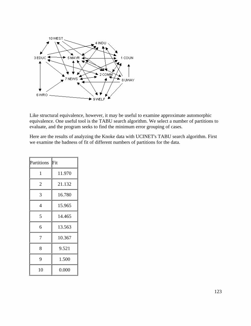
123

Like structural equivalence, however, it may be useful to examine approximate automorphicequivalence. One useful tool is the TABU search algorithm. We select a number of partitions toevaluate, and the program seeks to find the minimum error grouping of cases.

Here are the results of analyzing the Knoke data with UCINET's TABU search algorithm. Firstwe examine the badness of fit of different numbers of partitions for the data.

Partitions Fit

1 11.970

2 21.132

3 16.780

4 15.965

5 14.465

6 13.563

7 10.367

8 9.521

9 1.500

10 0.000

124

notes: There is no "right" answer about how many automorphisms there are here. There are twotrivial answers: those that group all the cases together into one partition and those that separateeach case into it's own partition. In between, one might want to follow the logic of the "scree"plot from factor analysis to select a meaningful number of partitions. Look first at the results forthree partitions:

AUTOMORPHIC BLOCKMODELS VIA TABU SEARCHDiagonal valid? NOUse geodesics? YESFit: 16.780Block Assignments: 1: COUN COMM EDUC INDU NEWS UWAY WELF WEST 2: WRO 3: MAYRBlocked Distance Matrix 1 1 2 3 4 0 8 7 9 6 5 C C E I W U N W W M --------------------------- 1 COUN | 1 2 2 2 2 1 1 | 3 | 1 | 2 COMM | 1 1 1 2 1 1 1 | 2 | 1 | 3 EDUC | 2 1 1 1 2 1 2 | 1 | 1 | 4 INDU | 1 1 2 2 2 1 2 | 3 | 1 | 10 WEST | 1 1 1 2 2 1 2 | 2 | 1 | 8 UWAY | 1 1 2 1 2 1 1 | 3 | 1 | 7 NEWS | 2 1 2 1 2 2 2 | 3 | 1 | 9 WELF | 2 1 2 2 2 2 1 | 3 | 1 | --------------------------- 6 WRO | 3 2 1 2 2 3 1 1 | | 2 | --------------------------- 5 MAYR | 1 1 1 1 1 1 1 1 | 2 | | ---------------------------

note: the rows and columns for WRO have similar variances (high ones), and that the rows andcolumns for the mayor have similar variances (low ones). It appears that the algorithm has donea good job of blocking the matrix to produce rows and columns with similar variance withinblocks. One very simple (but not too crude) view of the data is that the mayor and the WRO arequite unique, and have similar relationships with more-or-less interchangeable actors in the largeremaining group.

Of course, with more partitions, one can achieve better goodness-of-fit. The analysts will have tojudge for themselves, given the purposes of their study, whether the better fit is a better model --or just a more complicated one. Here's the result for seven partitions:

125

AUTOMORPHIC BLOCKMODELS VIA TABU SEARCHDiagonal valid? NOUse geodesics? YESFit: 10.367Block Assignments: 1: COUN INDU NEWS WELF 2: WRO 3: UWAY 4: EDUC 5: COMM 6: WEST 7: MAYRBlocked Distance Matrix 1 1 7 9 4 6 8 3 2 0 5 C N W I W U E C W M ----------------------------------- 1 COUN | 1 1 2 | 3 | 2 | 2 | 1 | 2 | 1 | 7 NEWS | 2 2 1 | 3 | 2 | 2 | 1 | 2 | 1 | 9 WELF | 2 1 2 | 3 | 2 | 2 | 1 | 2 | 1 | 4 INDU | 1 1 2 | 3 | 2 | 2 | 1 | 2 | 1 | ----------------------------------- 6 WRO | 3 1 1 2 | | 3 | 1 | 2 | 2 | 2 | ----------------------------------- 8 UWAY | 1 1 1 1 | 3 | | 2 | 1 | 2 | 1 | ------------------------------------ 3 EDUC | 2 1 2 1 | 1 | 2 | | 1 | 1 | 1 | ----------------------------------- 2 COMM | 1 1 1 1 | 2 | 1 | 1 | | 2 | 1 | ----------------------------------- 10 WEST | 1 1 2 2 | 2 | 2 | 1 | 1 | | 1 | ----------------------------------- 5 MAYR | 1 1 1 1 | 2 | 1 | 1 | 1 | 1 | | -----------------------------------

notes: In this case, further partitions of the data result in separating additional individual actorsfrom the larger "center." This need not be the case. Factions and splits of partitions, as well asseparation of individual actors could have resulted. We are left with a view of this network asone in which there is a core of about 1/2 of the actors who are more or less substitutable in theirrelations with a number (six, in the result shown) of other positions.

Summary of chapter 10

The kind of equivalence expressed by the notion of automorphism falls between structural andregular equivalence, in a sense. Structural equivalence means that individual actors can besubstituted one for another. Automorphic equivalence means that sub-structures of graphs can besubstituted for one another. As we will see next, regular equivalence goes further still, and seeksto deal with classes or types of actors--where each member of any class has similar relations withsome member of each other.

126

The notion of structural equivalence corresponds well to analyses focusing on how individualsare embedded in networks -- or network positional analysis. The notion of regular equivalencefocuses our attention on classes of actors, or "roles" rather than individuals or groups.Automorphic equivalence analysis falls between these two more conventional foci, and has notreceived as much attention in empirical research. Still, the search for multiple substitutable sub-structures in graphs (particularly in large and complicated ones) may reveal that the complexityof very large structures is more apparent than real; sometimes very large structures aredecomposable (or partially so) into multiple similar smaller ones.

127

11. Regular Equivalence

Defining regular equivalence

Regular equivalence is the least restrictive of the three most commonly used definitions ofequivalence. It is, however, probably the most important for the sociologist. This is because theconcept of regular equivalence, and the methods used to identify and describe regularequivalence sets correspond quite closely to the sociological concept of a "role." The notion ofsocial roles is a centerpiece of most sociological theorizing.

Formally, "Two actors are regularly equivalent if they are equally related to equivalent others."(Borgatti, Everett, and Freeman, 1996: 128). That is, regular equivalence sets are composed ofactors who have similar relations to members of other regular equivalence sets. The concept doesnot refer to ties to specific other actors, or to presence in similar sub-graphs; actors are regularlyequivalent if they have similar ties to any members of other sets.

The concept is actually easier to grasp intuitively than formally. Susan is the daughter of Inga.Deborah is the daughter of Sally. Susan and Deborah form a regular equivalence set becauseeach has a tie to a member of the other set. Inga and Sally form a set because each has a tie to amember of the other set. In regular equivalence, we don't care which daughter goes with whichmother; what is identified by regular equivalence is the presence of two sets (which we mightlabel "mothers" and "daughters"), each defined by it's relation to the other set. Mothers aremothers because they have daughters; daughters are daughters because they have mothers.

Uses of the concept

Most approaches to social positions define them relationally. For Marx, capitalists can only existif there are workers, and vice versa. The two "roles" are defined by the relation between them(i.e. capitalists expropriate surplus value from the labor power of workers). Husbands and wives;men and women; minorities and majorities; lower caste and higher caste; and most other rolesare defined relationally.

The regular equivalence approach is important because it provides a method for identifying"roles" from the patterns of ties present in a network. Rather than relying on attributes of actorsto define social roles and to understand how social roles give rise to patterns of interaction,regular equivalence analysis seeks to identify social roles by identifying regularities in thepatterns of network ties -- whether or not the occupants of the roles have names for theirpositions.

Regular equivalence analysis of a network then can be used to locate and define the nature ofroles by their patterns of ties. The relationship between the roles that are apparent from regularequivalence analysis and the actor's perceptions or naming of their roles can be problematic.What actors label others with role names and the expectations that they have toward them as aresult (i.e. the expectations or norms that go with roles) may pattern -- but not wholly determine

128

actual patterns of interaction. Actual patterns of interaction, in turn, are the regularities out ofwhich roles and norms emerge.

These ideas: interaction giving rise to culture and norms, and norms and roles constraininginteraction, are at the core of the sociological perspective. The identification and definition of"roles" by the regular equivalence analysis of network data is possibly the most importantintellectual development of social network analysis.

Finding Equivalence Sets

The formal definition says that two actors are regularly equivalent if they have similar patterns ofties to equivalent others. Consider two men. Each has children (though they have differentnumbers of children, and, obviously have different children). Each has a wife (though again,usually different persons fill this role with respect to each man). Each wife, in turn also haschildren and a husband (that is, they have ties with one or more members of each of those sets).Each child has ties to one or more members of the set of "husbands" and "wives."

In identifying which actors are "husbands" we do not care about ties between members of this set(actually, we would expect this block to be a zero block, but we really don't care). What isimportant is that each "husband" have at least one tie to a person in the "wife" category and atleast one person in the "child" category. That is, husbands are equivalent to each other becauseeach has similar ties to some member of the sets of wives and children.

But there would seem to be a problem with this fairly simple definition. If the definition of eachposition depends on its relations with other positions, where do we start?

There are a number of algorithms that are helpful in identifying regular equivalence sets.UCINET provides some methods that are particularly helpful for locating approximatelyregularly equivalent actors in valued, multi-relational and directed graphs. Some simplermethods for binary data can be illustrated directly.

Consider, again, the Wasserman-Faust example network. Imagine, however, that this is a pictureof order-giving in a simple hierarchy. That is, all ties are directed from the top of the diagramdownward. We will find a regular equivalence characterization of this diagram.

For a first step, characterize each position as either a "source" (an actor that sends ties, but does

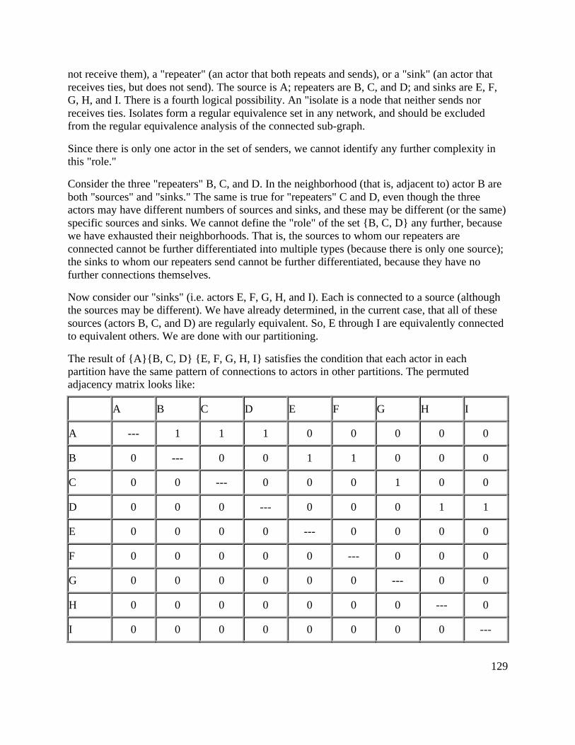
129

not receive them), a "repeater" (an actor that both repeats and sends), or a "sink" (an actor thatreceives ties, but does not send). The source is A; repeaters are B, C, and D; and sinks are E, F,G, H, and I. There is a fourth logical possibility. An "isolate is a node that neither sends norreceives ties. Isolates form a regular equivalence set in any network, and should be excludedfrom the regular equivalence analysis of the connected sub-graph.

Since there is only one actor in the set of senders, we cannot identify any further complexity inthis "role."

Consider the three "repeaters" B, C, and D. In the neighborhood (that is, adjacent to) actor B areboth "sources" and "sinks." The same is true for "repeaters" C and D, even though the threeactors may have different numbers of sources and sinks, and these may be different (or the same)specific sources and sinks. We cannot define the "role" of the set {B, C, D} any further, becausewe have exhausted their neighborhoods. That is, the sources to whom our repeaters areconnected cannot be further differentiated into multiple types (because there is only one source);the sinks to whom our repeaters send cannot be further differentiated, because they have nofurther connections themselves.

Now consider our "sinks" (i.e. actors E, F, G, H, and I). Each is connected to a source (althoughthe sources may be different). We have already determined, in the current case, that all of thesesources (actors B, C, and D) are regularly equivalent. So, E through I are equivalently connectedto equivalent others. We are done with our partitioning.

The result of {A}{B, C, D} {E, F, G, H, I} satisfies the condition that each actor in eachpartition have the same pattern of connections to actors in other partitions. The permutedadjacency matrix looks like:

A B C D E F G H I

A --- 1 1 1 0 0 0 0 0

B 0 --- 0 0 1 1 0 0 0

C 0 0 --- 0 0 0 1 0 0

D 0 0 0 --- 0 0 0 1 1

E 0 0 0 0 --- 0 0 0 0

F 0 0 0 0 0 --- 0 0 0

G 0 0 0 0 0 0 --- 0 0

H 0 0 0 0 0 0 0 --- 0

I 0 0 0 0 0 0 0 0 ---

130

It is useful to block this matrix and show it's image. Here, however, we will use some specialrules for determining zero and 1 blocks. If a block is all zeros, it will be a zero block. If eachactor in a partition has a tie to any actor in another, then we will define the joint block as a 1-block. Bear with me a moment. The image, using this rule is:

A B,C,D E,F,G,H,I

A --- 1 0

B,C,D 0 --- 1

E,F,G,H,I 0 0 ---

A sends to one or more of BCD but to none of EFGHI. BCD do not send to A, but each of BCDsends to at least one of EFGHI. None of EFGHI send to any of A, or of BCD. The image, in fact,displays the characteristic pattern of a strict hierarchy: ones on the first off-diagonal vector andzeros elsewhere. The rule of defining a 1 block when each actor in one partition has arelationship with any actor in the other partition is a way of operationalizing the notion that theactors in the first set are equivalent if they are connected to equivalent actors (i.e. actors in theother partition), without requiring (or prohibiting) that they be tied to the same other actors. Thisimage rule is the basis of the tabu search algorithm. The neighborhood search algorithm is thebasis for REGE's approach to categorical data (see discussions and examples below).

To review: we begin a neighborhood search by characterizing each actor as a source, repeater,sink, or isolate. Looking within each category, we then examine the kinds of actors that arepresent in the neighborhood of each of the actors in our initial partitions. If the kinds of actorspresent in each of their neighborhoods are the same, we are finished and can move on to the nextinitial group; if the actors have different neighborhood composition, we can sub-divide them, andrepeat the process. In principle, searching neighborhoods can continue outward from each actoruntil paths of all lengths have been examined. In practice, analysts go no further than 3 steps. Formost problems, differences in the composition of actor's neighborhoods more distant than thatare not likely to be substantively important.

The neighborhood search rule works well for binary, directed data. It can be extended to integervalued and multi-relational data (REGE categorical algorithm). If the strength of directed tieshas been measured (or if one wants to use the reciprocal of the geodesic distance between actorsas a proxy for tie strength), the REGE continuous algorithm can be applied to iteratively re-weight in the neighborhood search to identify approximately regularly equivalent actors.

Many sets of network data show non-directed ties. Applying regular equivalence algorithms canbe troublesome in these cases. Consider the Wasserman-Faust network in its undirected form.

131

Without noting direction, we cannot divide the data into "sources" "repeaters" and "sinks," so theneighborhood search idea breaks down. In this case, it might make sense to examine the geodesicdistance matrix, rather than the adjacency matrix. One can then use categorical REGE (whichtreats each distinct geodesic distance value as a qualitatively different neighbor). Or, one can usecontinuous REGE (probably a more reasonable choice), regarding the inverse of distance as ameasure of tie strength.

Let's look at some examples of these approaches with real data. First, we will illustrate the basicneighborhood search approach with REGE categorical. Then, we will compare the categoricaland continuous treatments of geodesics as values for an undirected graph. Lastly, we will applythe tabu search method to some directed binary data.

Categorical REGE for directed binary data (Knoke information exchange)

The Knoke information exchange network is directed and binary, though many ties arereciprocated.

The REGE algorithm, when applied to binary data, adopts the approach of first categorizingactors as sources, repeaters, and sinks. It then attempts to sub-divide the actors in each of thesecategories according to the types of actors in their neighborhood. The process continues (usuallynot for long) until all actors are divided, on no further differentiation can be drawn by extendingthe neighborhood. Here are the results:

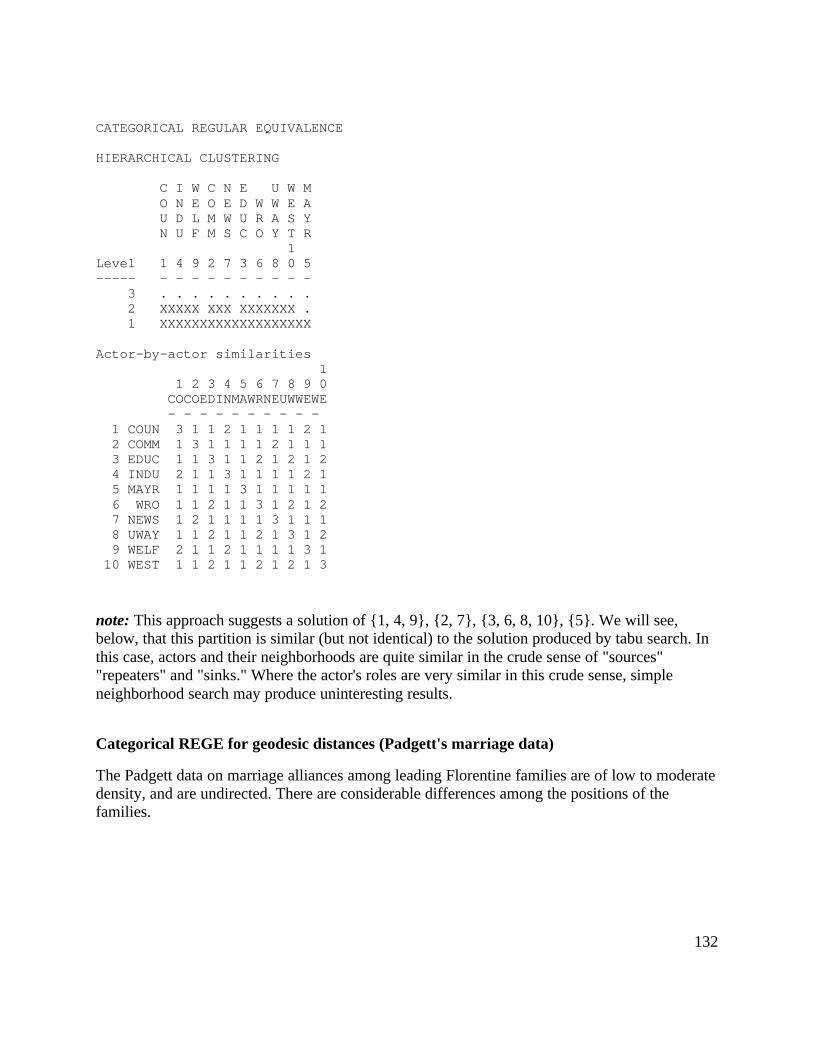
132

CATEGORICAL REGULAR EQUIVALENCE

HIERARCHICAL CLUSTERING

C I W C N E U W M O N E O E D W W E A U D L M W U R A S Y N U F M S C O Y T R 1Level 1 4 9 2 7 3 6 8 0 5----- - - - - - - - - - - 3 . . . . . . . . . . 2 XXXXX XXX XXXXXXX . 1 XXXXXXXXXXXXXXXXXXX

Actor-by-actor similarities 1 1 2 3 4 5 6 7 8 9 0 COCOEDINMAWRNEUWWEWE - - - - - - - - - - 1 COUN 3 1 1 2 1 1 1 1 2 1 2 COMM 1 3 1 1 1 1 2 1 1 1 3 EDUC 1 1 3 1 1 2 1 2 1 2 4 INDU 2 1 1 3 1 1 1 1 2 1 5 MAYR 1 1 1 1 3 1 1 1 1 1 6 WRO 1 1 2 1 1 3 1 2 1 2 7 NEWS 1 2 1 1 1 1 3 1 1 1 8 UWAY 1 1 2 1 1 2 1 3 1 2 9 WELF 2 1 1 2 1 1 1 1 3 1 10 WEST 1 1 2 1 1 2 1 2 1 3

note: This approach suggests a solution of {1, 4, 9}, {2, 7}, {3, 6, 8, 10}, {5}. We will see,below, that this partition is similar (but not identical) to the solution produced by tabu search. Inthis case, actors and their neighborhoods are quite similar in the crude sense of "sources""repeaters" and "sinks." Where the actor's roles are very similar in this crude sense, simpleneighborhood search may produce uninteresting results.

Categorical REGE for geodesic distances (Padgett's marriage data)

The Padgett data on marriage alliances among leading Florentine families are of low to moderatedensity, and are undirected. There are considerable differences among the positions of thefamilies.

133

The categorical REGE algorithm can be used to identify regularly equivalent actors by treatingthe elements of the geodesic distance matrix as describing "types" of ties -- that is differentgeodesic distances are treated as "qualitatively" rather than "quantitatively" different. Two nodesare more equivalent if each has an actor in their neighborhood of the same "type" in this case,that means they are similar if they each have an actor that is at the same geodesic distance fromthemselves. With many data sets, the levels of similarity of neighborhoods can turn out to bequite high -- and it may be difficult to differentiate the positions of the actors on "regular"equivalence grounds.

CATEGORICAL REGULAR EQUIVALENCE

WARNING: Data converted to geodesic distances before processing.

HIERARCHICAL CLUSTERING

A B C L T C A B A G A S O C S A R R I S U M P A R I T L I B S T G A B M E L N A R B D A C E I D E E P R P V A I O I O D H L N A R D A U U I B U Z Z L O E L O G T I Z Z C A U O Z Z F R R A R N E C Z Z C T O L I I I I I N I I S I I I I I N

1 1 1 1 1 1 1Level 1 5 2 3 3 4 5 6 7 8 9 0 1 2 4 6----- - - - - - - - - - - - - - - - - 3 . . . . . . . . . . . . . . . . 2 XXX XXX . . . . . . . . . . . . 1 XXXXXXXXXXXXXXXXXXXXXXXXXXXXXXX

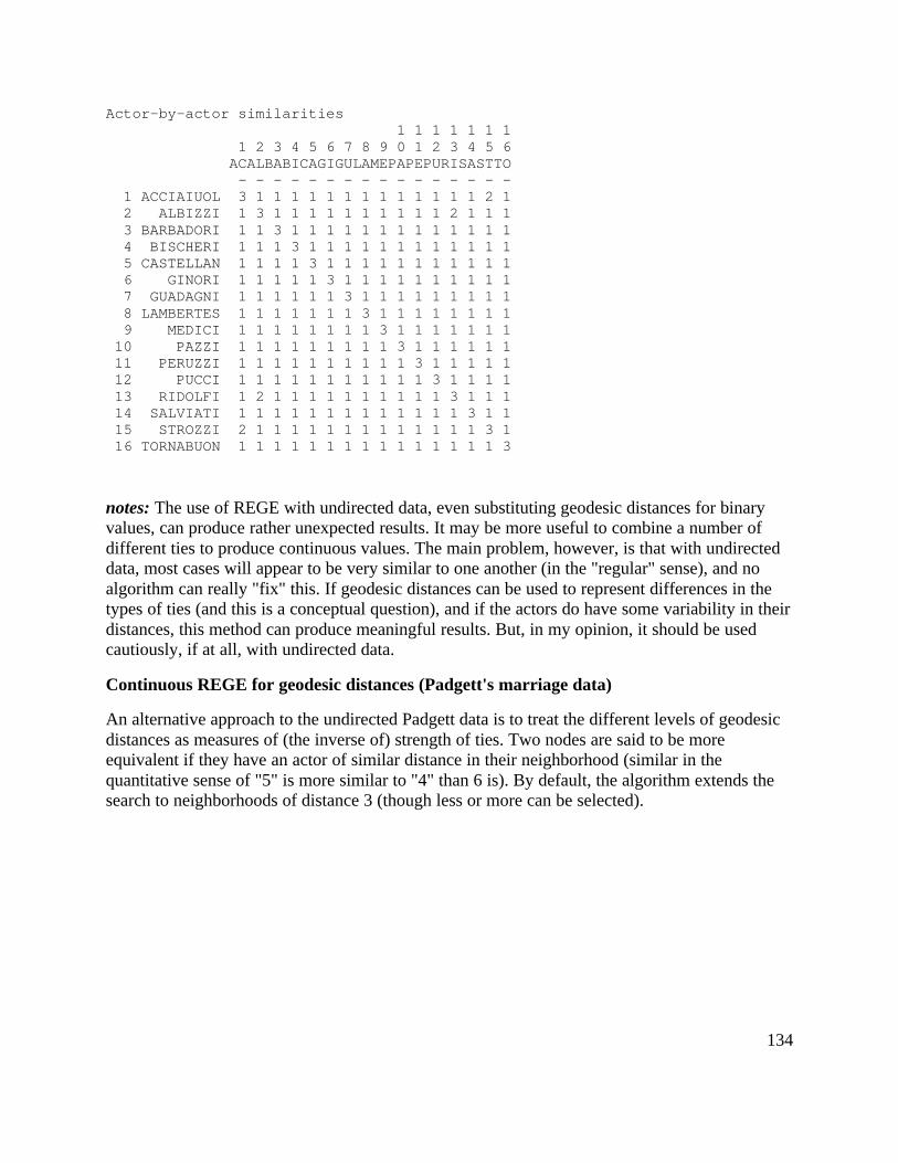
134

Actor-by-actor similarities 1 1 1 1 1 1 1 1 2 3 4 5 6 7 8 9 0 1 2 3 4 5 6 ACALBABICAGIGULAMEPAPEPURISASTTO - - - - - - - - - - - - - - - - 1 ACCIAIUOL 3 1 1 1 1 1 1 1 1 1 1 1 1 1 2 1 2 ALBIZZI 1 3 1 1 1 1 1 1 1 1 1 1 2 1 1 1 3 BARBADORI 1 1 3 1 1 1 1 1 1 1 1 1 1 1 1 1 4 BISCHERI 1 1 1 3 1 1 1 1 1 1 1 1 1 1 1 1 5 CASTELLAN 1 1 1 1 3 1 1 1 1 1 1 1 1 1 1 1 6 GINORI 1 1 1 1 1 3 1 1 1 1 1 1 1 1 1 1 7 GUADAGNI 1 1 1 1 1 1 3 1 1 1 1 1 1 1 1 1 8 LAMBERTES 1 1 1 1 1 1 1 3 1 1 1 1 1 1 1 1 9 MEDICI 1 1 1 1 1 1 1 1 3 1 1 1 1 1 1 1 10 PAZZI 1 1 1 1 1 1 1 1 1 3 1 1 1 1 1 1 11 PERUZZI 1 1 1 1 1 1 1 1 1 1 3 1 1 1 1 1 12 PUCCI 1 1 1 1 1 1 1 1 1 1 1 3 1 1 1 1 13 RIDOLFI 1 2 1 1 1 1 1 1 1 1 1 1 3 1 1 1 14 SALVIATI 1 1 1 1 1 1 1 1 1 1 1 1 1 3 1 1 15 STROZZI 2 1 1 1 1 1 1 1 1 1 1 1 1 1 3 1 16 TORNABUON 1 1 1 1 1 1 1 1 1 1 1 1 1 1 1 3

notes: The use of REGE with undirected data, even substituting geodesic distances for binaryvalues, can produce rather unexpected results. It may be more useful to combine a number ofdifferent ties to produce continuous values. The main problem, however, is that with undirecteddata, most cases will appear to be very similar to one another (in the "regular" sense), and noalgorithm can really "fix" this. If geodesic distances can be used to represent differences in thetypes of ties (and this is a conceptual question), and if the actors do have some variability in theirdistances, this method can produce meaningful results. But, in my opinion, it should be usedcautiously, if at all, with undirected data.

Continuous REGE for geodesic distances (Padgett's marriage data)

An alternative approach to the undirected Padgett data is to treat the different levels of geodesicdistances as measures of (the inverse of) strength of ties. Two nodes are said to be moreequivalent if they have an actor of similar distance in their neighborhood (similar in thequantitative sense of "5" is more similar to "4" than 6 is). By default, the algorithm extends thesearch to neighborhoods of distance 3 (though less or more can be selected).

135

REGULAR EQUIVALENCE VIA WHITE/REITZ REGE ALGORITHM

REGE similarities (3 iterations)

1 2 3 4 5 6 7 8 9 10 11 12 13 14 15 16 ACCIALBIBARBBISCCASTGINOGUADLAMBMEDIPAZZPERUPUCCRIDOSALVSTROTORN --- --- --- --- --- --- --- --- --- --- --- --- --- --- --- --- 1 ACCIAIUOL 100 93 43 52 51 29 64 33 46 60 45 0 91 67 92 73 2 ALBIZZI 93 100 53 62 62 42 73 47 56 72 56 0 94 81 94 79 3 BARBADORI 43 53 100 96 95 70 95 98 91 71 96 0 52 94 57 94 4 BISCHERI 52 62 96 100 99 76 99 98 97 71 100 0 67 94 70 98 5 CASTELLAN 51 62 95 99 100 76 98 97 97 70 99 0 66 93 70 97 6 GINORI 29 42 70 76 76 100 75 83 73 92 78 0 54 74 53 79 7 GUADAGNI 64 73 95 99 98 75 100 97 97 71 99 0 76 93 79 97 8 LAMBERTES 33 47 98 98 97 83 97 100 91 84 98 0 47 95 53 96 9 MEDICI 46 56 91 97 97 73 97 91 100 66 97 0 62 86 65 9210 PAZZI 60 72 71 71 70 92 71 84 66 100 73 0 72 73 77 7811 PERUZZI 45 56 96 100 99 78 99 98 97 73 100 0 60 94 64 9812 PUCCI 0 0 0 0 0 0 0 0 0 0 0 100 0 0 0 013 RIDOLFI 91 94 52 67 66 54 76 47 62 72 60 0 100 76 100 8614 SALVIATI 67 81 94 94 93 74 93 95 86 73 94 0 76 100 78 9315 STROZZI 92 94 57 70 70 53 79 53 65 77 64 0 100 78 100 8716 TORNABUON 73 79 94 98 97 79 97 96 92 78 98 0 86 93 87 100

HIERARCHICAL CLUSTERING OF EQUIVALENCE MATRIX

A B L C T C S A A G A B O C A R S A R M U S I P R I L I T G L M B B A T S E N P A B D R I P V E A E D E C R A U I I O O N A I D D R A L H U B C U Z L Z O Z A I O T G L E Z U C O Z F Z R Z T C R E N A R Z O I L I I I I I I I I S I N I I N

1 1 1 1 1 1 1 Level 2 1 2 3 5 6 0 4 9 3 8 7 5 4 1 6------ - - - - - - - - - - - - - - - -99.860 . . . . . . . . . . . . . XXX .99.787 . . . XXX . . . . . . . . XXX .99.455 . . . XXX . . . . . . . XXXXX .98.609 . . . XXX . . . . . . XXXXXXX .97.895 . . . XXX . . . . XXX XXXXXXX .97.676 . . . XXX . . . . XXX XXXXXXXXX96.138 . . . XXX . . . . XXXXXXXXXXXXX93.756 . . XXXXX . . . . XXXXXXXXXXXXX93.673 . . XXXXX . . . XXXXXXXXXXXXXXX92.796 . . XXXXX . . XXXXXXXXXXXXXXXXX92.059 . . XXXXX XXX XXXXXXXXXXXXXXXXX91.911 . XXXXXXX XXX XXXXXXXXXXXXXXXXX75.816 . XXXXXXX XXXXXXXXXXXXXXXXXXXXX67.386 . XXXXXXXXXXXXXXXXXXXXXXXXXXXXX 0.000 XXXXXXXXXXXXXXXXXXXXXXXXXXXXXXX

136

notes: The continuous REGE algorithm applied to geodesic distances for the undirected data isprobably a better choice than the categorical approach. The result still shows very high regularequivalence among the actors, and the solution is only modestly similar to that of the categoricalapproach.

The Knoke bureaucracies information exchange network analyzed by Tabu search

Above, we examined the Knoke information network using neighborhood search. The tabumethod is an iterative search for a permutation and partition of the graph (given a prior decisionabout how may partions) that produces the fewest possible "exceptions" to zero and one blockcoding for regular equivalence. That is, blocks are zero if all entries are zero and one if there is atleast one element in each row and column. Here we apply this method to the same data set thatwe used earlier to look at the simple neighborhood search approach. The result is:

REGULAR BLOCKMODELS VIA TABU SEARCH

Number of blocks: 4

Fit: 2.000

Block Assignments:

1: COMM MAYR 2: EDUC WRO WEST 3: COUN INDU NEWS WELF 4: UWAY

137

Blocked Adjacency Matrix

1 5 2 6 0 3 4 7 1 9 8 M C W W E I N C W U ----------------------------- 5 MAYR | 1 | 1 1 | 1 1 1 1 | 1 | 2 COMM | 1 | 1 | 1 1 1 1 | 1 | ----------------------------- 6 WRO | | 1 | 1 1 | | 10 WEST | 1 1 | 1 | 1 1 | | 3 EDUC | 1 1 | 1 1 | 1 1 | | ----------------------------- 4 INDU | 1 1 | | 1 1 | | 7 NEWS | 1 1 | | 1 | | 1 COUN | 1 1 | | 1 1 | | 9 WELF | 1 1 | | 1 | | ----------------------------- 8 UWAY | 1 1 | | 1 1 1 1 | | -----------------------------

notes: The method produces a fit statistic, and solutions for different numbers of partitionsshould be compared. In the current case, a 5 group model fits somewhat better than the 4 groupsolution shown here. The four group solution is reported, so that it can be compared to theneighborhood search result, above.

The blocked adjacency matrix for the 4 group solution is, however, quite convincing. Of the 12blocks of interest (the blocks on the diagonal are not usually treated as relevant to "role"analysis) 10 satisfy the rules for zero or one blocks perfectly.

The solution is also an interesting one substantively. The first set (2,5) for example, are pure"repeaters" sending and receiving from all other roles. The set { 6, 10, 3 } send to only two othertypes (not all three other types) and receive from only one other type. And so on.

The tabu search method can be very useful, and usually produces quite nice results. It is aniterative search algorithm, however, and can find local solutions. Many networks have more thanone valid partitioning by regular equivalence, and there is no guarantee that the algorithm willalways find the same solution. It should be run a number of times with different startingconfigurations.

Summary of chapter 11

The regular equivalence concept is a very important one for sociologists using social networkmethods, because it accords well with the notion of a "social role." Two actors are regularlyequivalent if they are equally related to equivalent (but not necessarily the same, or same numberof) equivalent others. Regular equivalencies can be exact or approximate. Unlike the structuraland automorphic equivalence definitions, there may be many valid ways of classifying actorsinto regular equivalence sets for a given graph -- and more than one may be meaningful.

138

There are a number of algorithmic approaches for performing regular equivalence analysis. Allare based on searching the neighborhoods of actors and profiling these neighborhoods by thepresence of actors of other "types." To the extent that actors have similar "types" of actors atsimilar distances in their neighborhoods, they are regularly equivalent. This seemingly loosedefinition can be translated quite precisely into zero and one-block rules for making imagematrices of proposed regular equivalence blockings. The "goodness" of these images is perhapsthe best test of a proposed regular equivalence partitioning. And, the images themselves are thebest description of the nature of each "role" in terms of its' expected pattern of ties with otherroles.

We have only touched the surface of regular equivalence analysis, and the analysis of roles innetworks. One major extensions that make role analysis far richer is the inclusion of multiplekinds of ties (that is, stacked or pooled matrices of ties). Another extension is "role algebra"which seeks to identify "underlying" or "generator" or "master" relations from the patterns of tiesin multiple tie networks (rather than simply stacking them up or adding them together).

139

A Working Bibliography on Social Network Analysis Methods

• Alba, Richard D. 1973. "A graph-theoretic definition of a sociometric clique" Journal ofMathematical Sociology, 3: 113-126

• Alba, Richard D. and Gwen Moore. 1983. "Elite social circles" Chapter 12 in Burt andMinor (eds). Applied network analysis: A methodological introduction. Beverly Hills:Sage.

• Anheier, Helmut K. 1987. "Structural analysis and strategic research design: Studyingpoliticized interorganizational networks" Sociological Forum 2: 563-582

• Arabie, P., S.A. Boorman, and P.R. Levitt. 1978. "Constructing blockmodels: How andwhy" Journal of Mathematical Psychology, Vol. 17: 21-63

• Baker, Wayne E. 1986. "Three-dimensional blockmodels" Journal of MathematicalSociology, 12: 191-223.

• Baker, Wayne E. 1990. "Market Networks and Corporate Behavior" American Journal ofSociology. 96: 589-625.

• Barnes, J.A. 1983. "Graph theory in network analysis" Social Networks 5: 235-244.

• Berkowitz, S.D. 1988. "Markets and market-areas: Some preliminary formulations" pp.261-303 in Wellman and Berkowitz (eds.) Social structures: A network approach.Cambridge: Cambridge University Press

• Berkowitz, S.D. 1988. Afterword: Toward a formal structural sociology, pp. 477-497 inWellman and Berkowitz (eds.) Social structures: A network approach. Cambridge:Cambridge University Press.

• Berkowitz, S.D. 1982. An introduction to structural analysis: The network approach tosocial research Toronto: Butterworths

• Berkowitz, S.D., Peter J. Carrington, Yehuda Kotowitz, and Leonard Waverman. 1978-79. The determination of enterprise groupings through combined ownership anddirectoship ties, Social Networks 1: 391-413.

• Blau, Peter and Robert K. Merton. 1981. Continuities in structural inquiry London andBeverly Hills: Sage.

• Blau, Peter. 1981. Introduction: Diverse views of social structure and their commondenominator. in Blau and merton (eds.) Continuities in structural inquiry. London andBeverly Hills: Sage.

• Bodemann, Y. Michal. 1988. Relations of production and class rule: The hidden basis ofpatron-clientage. pp. 198-220 in Wellman and Berkowitz (eds.) Social structrues: A

140

network approach. Cambridge: Cambridge University Press

• Bonacich, Phillip. 1972. Technique for analyzing overlapping memberships. in HerbertCostner (ed.) Sociological Methodology 1972. San Francisco: Jossey-Bass

• Bonacich, Phillip. 1972. Factoring and weighting approaches to status scores and cliquedetection, Journal of Mathematical Sociology, 2: 113-120

• Boorman, S.A. 1975. A combinatorial optimization model for transmission of jobinformation through contact networks, Bell Journal of Economics, 6: 216-249

• Borgatti, Steven, Martin Everett, and Linton Freeman. 1992. UCINET IV Version 1.0User's Guide. Columbia, SC: Analytic Technologies.

• Bott, Elizabeth. 1957. Family and social network London: Tavistock Publications

• Bougon, Michel, Karl Weick, and Din Binkhorst. 1977. Cognition in organizations: Ananlaysis of the Utrecht jazz orchestra, Administrative Science Quarterly, Vol. 22: 606-639

• Boyd, John Paul, John H. Haehl and Lee D. Sailer. 1972. Kinship systems and inversesemigroups, Journal of Mathematical Sociology, 2: 37-61

• Breiger, Ronald. 1979. Toward an operational theory of community elite structure,Quality and Quantity, 13: 21-47.

• Breiger, Ronald L. and Philippa E. Pattison. 1978. The joint role structure of twocommunities' elites, Sociological Methods and Research, 7: 213-26.

• Breiger, Ronald L. and Philippa E. Pattison. 1986. Cumulated social roles: The duality ofpersons and their algebras, Social Networks, 8: 215-256.

• Breiger, R.L. 1976. Career attributes and network structure: A blockmodel study of a bio-medical research specialty, American Sociological Review, 41: 117-135

• Breiger, Ronald L. 1988. The duality of persons and groups. pp. 83-98 in Wellman andBerkowitz (eds.) Social structures: A network approach. Cambridge: CambridgeUniversity Press.

• Brym, Robert J. 1988. Structural location and ideological divergence: Jewish Marxistintellectuals in turn-of-the-century Russia. pp. 332-358 in Wellman and Berkowitz (eds.)Social structures: A network approach. Cambridge: Cambridge University Press.

• Burkhardt, Marlene E. and Daniel J. Brass. 1989. Changing patterns or patterns ofchange: A longitudinal investigation of the interplay of technology, structure, and power,Pennsylvania State University, mimeo.

• Burt, Ronald S. 1982. Toward a Structural Theory of Action. New York: Academic Press.

141

• Burt, Ronald S. 1983. Distinguishing relational contents. pp. 35-74 in Burt and Minor(eds.) Applied network analysis: A methodological introduction. Beverly Hills: Sage

• Burt, Ronald S. 1983. Network data from informant interviews. Chapter 7 in Burt andMinor (eds.) Applied network analysis: A methodological introduction

• Burt, Ronald S. 1983. Cohesion versus structural equivalence as a basis for networksubgroups. Chapter 13 in Burt and Minor (eds.) Applied network analysis: Amethodological introduction. Beverly Hills: Sage.

• Burt, Ronald and M.J. Minor (eds.) 1983. Applied network analysis: A methodologicalintroduction Beverly Hills: Sage

• Burt, Ronald S. 1982. Toward a structural theory of action: Network models of socialstructure, perception, and action. New York: Academic Press.

• Burt, Ronald S. 1983. Corporate profits and cooptation: networks of market constraintsand directorate ties in the American economy. New York: Academic Press.

• Burt, Ronald S. 1980. Models of network structure, Annual Review of Sociology 6: 79-141

• Burt, Ronald S. 1983. Network data from archival records. Chapter 8 in Burt and Minor(eds.) Applied network analysis: A methodological introduction. Beverly HIlls: Sage

• Burt, Ronald S. 1983. Range, Chapter 9 in Burt and Minor (eds.) Applied networkanalysis: A methodological introduction

• Burt, Ronald S. 1976. Position in networks, Social Forces, 55: 93-122.

• Burt, Ronald S. 1987. Social Contagion and Innovation. American Journal of Sociology.92: 1287-1335.

• Burt, Ronald S. 1992. Structural Holes: The Social Structure of Competition. Cambridge,MA: Harvard University Press.

• Carrington, Peter J. and Greg H. Heil. 1981. COBLOC: A heierarchical method forblocking network data, Journal of Mathematical Sociology, 8: 103-131

• Carrington, Peter J., Greg H. Heil, and Stephen D. Berkowitz. 1979-80. A goodness-of-fitindex for blockmodels, Social Networks, 2: 219-234

• Cartwright, Dorwin. 1979. Balance and clusterability: An overview, pp. 25-50 in P.Holland and S. Leinhardt (eds.) Perspectives on social network research. New York:Academic Press.

• Cartwright, Dorwin and Frank Harary. 1977. A graph theoretic approach to theinvestigation of system-environment relationships, Journal of Mathematical Sociology,

142

Vol. 5: 87-111.

• Cartwright, D. and F. Harary. 1956. Structural balance: A generalization of Heider'stheory, Psychological Review, 63: 277-92.

• Clawson, Dan and Alan Neustadtl. 1989. Interlocks, PACs, and Corporate Conservatism.American Journal of Sociology. 94: 749-73.

• Clawson, Dan, Alan Neustadtl, and James Bearden. 1986. The Logic of Business Unity:Corporate Contributions to the 1980 Congressional Elections. American SociologicalReview. 51: 797-811.

• Coleman, James, Elihu Katz, and Herbert Menzel. 1957. The diffusion of an innovationamong physicians, Sociometry, 20: 253-270

• Cook, Karen. 1982. Network structures from an exchange perspective, in Peter Marsdenand Nan Lin (eds.). Socal structre and network analysis. Beverly Hills: Sage

• Crane, Diana. 1969. Social structure in a group of scientists: A test of the 'Invisiblecollege' hypothesis, American Sociological Review, 34: 335-352

• Davis, J. 1963. Structural balance, mechanical solidarity, and interpersonal relations,American Journal of Sociology, 68: 444-62

• Davis, James A. 1967. Clustering and structural balance in graphs, Human Relations, 30:181-187

• Delany, John. 1988. Social networks and efficient resource allocation: Computer modelsof job vacancy allocation through contacts, pp. 430-451 in Wellman and Berkowitz(eds.). Social structures: A network approach. Cambridge: Cambridge University

• Doreian, Patrick. 1974. On the connectivity of social networks, Journal of MathematicalSociology, 3: 245-258.

• Doreian, Patrick. 1988. Equivalence in a social network, Journal of MathematicalSociology, 13: 243-282.

• Emirbayer, Musafa and Jeff Goodwin. 1994. Network analysis, culture, and the problemsof agency. American Journal of Sociology. 99: 1411-54.

• Erikson, Bonnie. 1988. The relational basis of attitudes, pp. 99-122 in Wellman andBerkowitz (eds.), Social structures: A network approach. Cambridge: CambridgeUniversity Press.

• Everett, M.G. 1982. Graph theoretic blockings K-Plexes and K-cutpoints, Journal ofMathematical Sociology, 9: 75-84

• Everett, Martin G. 1982. A graph theoretic blocking procedure for social networks, Social

143

Networks, 4: 147-167

• Everett, Martin and Juhani Nieminen. 1980. Partitions and homomorphisms in directedand undirected graphs, Journal of Mathematical Sociology, 7: 91-111

• Feinberg, S.E. and Wasserman, S. 1981. Categorical data analysis of single sociolmetricrelations, in S. Leinhardt (ed.) Sociolgical Methodology 1981. San Francisco: Jossey-Bass.

• Fernandez, Roberto M. and Roger V. Gould. 1994. A Dilemma of State Power:Brokerage and Influence in the National Health Policy Domain. American Journal ofSociology. 99: 1455-91.

• Fischer, Claude. 1982. To Dwell among Friends: Personal Networks in Town and City.Chicago: University of Chicago Press.

• Fiskel, Joseph. 1980. Dynamic evolution in societal networks, Journal of MathematicalSociology, 7: 27-46.

• Flament, C. 1963. Applications of graph theory to group structure Englewood Cliffs:Prentice-Hall

• Frank, Ove, Maureen Hallinan, and Krzysztof Nowicki. 1985. Clustering of dyaddistributions as a tool in network modeling, Journal of Mathematical Sociology, 11: 47-64

• Frank, Ove. 1980. Transitivity in stochastic graphs and digraphs, Journal ofMathematical Sociology, 7: 199-213

• Freeman, Linton C. 1984. Turning a profit from mathematics: The case of socialnetworks, Journal of Mathematical Sociology, 10: 343-360

• Freeman, Linton. 1979. Centrality in social networks: Conceptual clarification, SocialNetworks, 1: 215-39.

• French Jr., John R.P. 1956. A formal theory of social power, Psychological Review, 63:181-194

• Friedkin, Noah E. 1986. A formal theory of social power, Journal of MathematicalSociology, 12: 103-126

• Friedmann, Harriet. 1988. Form and substance in the analysis of the world economy, pp.304-326 in Wellman and Berkowitz (eds.) Social structures: A network approach.Cambridge: Cambridge University Press.

• Galaskiewicz, Joseph and Stanley Wasserman. 1981. Change in a Regional CorporateNetwork. American Sociological Review. 46: 475-84.

144

• Gould, Roger V. 1991. Multiple Networks and Mobilization in the Paris Commune,1871. American Sociological Review. 56: 716-29.

• Gould, Roger V. 1993. Collective Action and Network Structure. American Journal ofSociology. 58: 182-96.

• Gould, Roger V. 1993. Trade Cohesion, Class Unity, and Urban Insurrection: ArtisinalActivism in the Paris Commune. American Journal of Sociology. 98: 721-54.

• Granovetter, Mark. 1973. The strength of weak ties. American Journal of Sociology, 78:1360-80.

• Granovetter, Mark. 1985. Economic action and social structure: the problem ofembeddedness. American Journal of Sociology. 91: 481-510.

• Granovetter, Mark. 1994. Getting a Job. Cambridge, MA: Harvard University Press.

• Hage, Per and Frank Harary. 1983. Structural models in anthropology Cambridge:Cambridge University Press

• Harary, Frank and Helene J. Kommel. 1979. Matrix measures for transitivity and balance,Journal of Mathematical Sociology, Vol 6.: 199-210

• Harary, Frank. 1971. Demiarcs: An atomistic approach to relational systems and groupdynamics, Journal of Mathematical Sociology, Vol. 1: 195-205

• Harary, F., R. Norman, and D. Cartwright. 1965. Structural models New York: Wiley

• Heider, Fritz. 1979. On balance and attribution, pp: 11-24 in Holland, P. and S. LeinhardtPerspectives on Social Network research. New York: Academic Press.

• Hoivik, Tord and Nils Petter Gleditsch. 1975. Structural parameters of graphs: Atheoretical investigation, in Blalock et al. (eds.). Quantitative Sociology. New York:Academic Press.

• Holland, Paul W. and Samuel Leinhardt. 1977. A dynamic model for social networks,Journal of Mathematical Sociology, 5: 5-20

• Holland, Paul W. and Samuel Leinhardt (eds.) 1979. Perspectives on social networkresearch New York: Academic Press

• Holland, Paul W. and Samuel Leinhardt. 1976. Local structure in social networks, pp. 1-45 in David Heise (ed.) Sociological Methodology, 1976. San Francisco: Josey-Bass

• Howard, Leslie. 1988. Work and community in industrializing India, pp. 185-197 inWellman and Berkowitz (Eds.) Social structures: A network approach. Cambridge:Cambridge University Press.

145

• Howell, Nancy. 1988. Understanding simple social structure: Kinship units and ties, pp.62-82 in Wellman and Berkowitz (eds.) Social structures: A network approach.Cambridge: Cambridge University Press.

• Hubbell, Charles H. 1965. An input-output approach to clique identification, Sociolmetry,28: 377-399

• Knoke, David and Ronald S. Burt. 1983. Prominence, Chapter 10 in Burt and Minor(eds.) Applied network analysis: A methodological introduction. Beverly Hills: Sage

• Knoke, D. and J. H. Kuklinski. 1981. Network analysis Beverly Hills: Sage

• Krackhardt, David. 198.9 Graph theoretical dimensions of informal organizations,Washington, D.C. presented at the Academy of Management meetings.

• Laumann, Edward O. 1973. Bonds of Pluralism: The Form and Substance of UrbanSocial Networks. New York: Wiley.

• Laumann, Edward O., Peter V. Marsden, and Joseph Galaskiewicz. 1977. CommunityInfluence Structures: Extension and Replication of a Network Approach. AmericanJournal of Sociology. 83: 594-631.

• Laumann, Edward O., Peter V. Marsden and David Prensky. 1983. The boundaryspecification problem in network analysis, pp. 18-34 in Burt and Minor (eds.) Appliednetwork analysis: A methodological introduction. Beverly Hills: Sage.

• Laumann, Edward O. and Peter V. Marsden. 1982. Microstructural analysis ininterorganizational systems, Social Networks, 4: 329-48.

• Laumann, Edward O., et al. 1994. The Social Organization of Sexuality: Sexual Practicesin the United States. Chicago: University of Chicago Press.

• Leik, Robert K. and B.F. Meeker. 197?. Graphs, matrices, and structural balance, pp. 53-73 in Leik and Meeker. Mathematical Sociology. Englewood Cliffs: Prentice-Hall

• Leinhardt, Samuel (ed.) 1977. Social networks: A developing paradigm New York:Academic Press

• Levine, Joel H. 1972. The sphere of influence, American Sociological Review, 37: 14-27

• Levine, Joel H. and John Spadaro. 1988. Occupational mobility: A structural model, pp.452-476 in Wellman and Berkowitz (eds.) Social structures: A network approach.Cambridge: Cambridge University Press.

• Lorrain, Francoise and Harrison C. White. 1971. The structural equivalence ofindividuals in social networks, Journal of Mathematical Sociology, 1: 49-80.

• Mandel, Michael J. 1983. Local roles and social networks, American Sociological

146

Review, 48: 376-386

• Marsden, Peter and Nan Lin (eds.) 1982. Social structure and network analysis. BeverlyHills: Sage.

• Marwell, Gerald, Pamela Oliver, and Ralph Prahl. 1988. Social Networks and CollectiveAction: A Theory of the Critical Mass. III. American Journal of Sociology. 94: 502-34.

• Mayer, Thomas F. 1984. Parties and networks: Stochastic models for relationshipnetworks, Journal of Mathematical Sociology, 10: 51-103.

• McCallister, Lynne and Claude S. Fischer. 1983. A procedure for surveying personalnetworks, pp. 75-88 in Burt and Minor (eds.) Applied network analysis: Amethodological introduction. Beverly Hills: Sage

• Minor, Michael J. 1983. Panel data on ego networks: A longitudinal study of formerheroin addicts, chapter 4 in Burt and Minor (eds.) Applied network analysis: Amethodological introduction. Beverly Hills: Sage.

• Minor, Michael J. 1983. New directions in multiplexity analysis, Chapter 11 in Burt andMinor (Eds.) Applied network analysis: A methodological introduction. Beverly Hills:Sage

• Mintz, Beth and Michael Schwartz. 1981. Interlocking directorates and interest groupformation, American Sociological Review, 46: 851-69.

• Mintz, Beth and Michael Schwartz. 1985. The power structure of American businessChicago: University of Chicago Press.

• Mitchell, Clyde. 1969. Social networks in urban situations: Analyses of personalrelationships in central African towns Manchester: Manchester University Press.

• Mizruchi, Mark S. 1989. Similarity of Political Behavior among American Corporations.American Journal of Sociology. 95: 401-24.

• Mizruchi, Mark S., Peter Mariolis, Michael Schwartz, and Beth Mintz. 1986. Techniquesfor disaggregating centrality scores in social networks, pp. 26-48 in Nancy Tuma (ed.)Sociological Methodology 1986. San Francisco: Jossey-Bass.

• Neustadtl, Alan and Dan Clawson. 1988. Corporate Political Groupings: Does IdeologyUnify Business Political Behavior? American Sociological Review. 53: 172-90.

• Oliver, Melvin. 1988. The Urban Black Community as Network: Toward a SocialNetwork Perspective. Sociological Quarterly. 29: 623-645.

• Padgett, John F. and Christopher K. Ansell. 1993. Robust Action and the Rise of theMedici, 1400-1434. American Journal of Sociology. 98: 1259-1319.

147

• Peay, Edmund R. 1976. A note concerning the connectivity of social networks, Journalof Mathematical Sociology, 4: 319-321

• Peay, Edmund R. 1982. Structural models with qualitative values, Journal ofMathematical Sociology, 8: 161-192

• Rapoport, A. 1963. Mathematical models of social interaction, pp. 493-579 in R. Luce, R.Bush and E. Galanter (eds.), Handbook of mathematical psychology, Vol. II. New York:Wiley

• Rogers, Everett M. 1979. Network analysis of the diffusion of innovations, pp. 137-164in P. Holland and S. Leinhardt (eds.) Perspectives on social network research.

• Roy, William. 1983. The Interlocking Directorate Structure of the United States.American Sociological Review. 42: 248-57.

• Sailer, Lee Douglas. 1978. Structural equivalence: Meaning and definition, computationand application, Social Networks, I: 73-90

• Scott, John. 1991. Social Network Analysis: A Handbook. Newbury Park, CA: SagePublications.

• Seidman, Stephen B. 1985. Structural consequences of individual position in nondyadicsocial networks, Journal of Mathematical Psychology, 29: 367-386

• Smith, David A. and Douglas R. White n.d. Structure and dynamics of the globaleconomy: Network analysis of international trade 1965-1980, University of Caliornia,Irvine, mimeo.

• Snyder, David and Edward L. Kick. 1979. Structural position in the world system andeconomic growth 1955-1970: A multiple-network analysis of transnational interactions,American Journal of Sociology, 84: 1096-1126

• Stark, Rodney and William Sims Bainbridge. 1980. Networks of faith: Interpersonalbonds and recuritment to cults and sects, American Journal of Sociology, 85: 1376-95

• Tepperman, Lorne. 1988. Collective mobility and the persistence of dynasties, pp. 405-429 in Wellman and Berkowitz ( eds.) Social structures: A network approach.Cambridge: Cambridge University Press.

• Tilly, Charles. 1988. Misreading, then reading, nineteenth-century social change, pp.332-358 in Wellman and Berkowitz (eds.) Social structures: A network approach.Cambridge: Cambridge University Press.

• Travers, Jeffrey and Stanley Milgram. 1969. An experimental study of the small worldproblem, Sociometry 32: 425-443

• Turk, Herman. 1970. Interorganizational networks in urban society: Initial perspectives

148

and comparative research, American Sociological Review, 35: 1-20.

• Uehara, Edwina. 1990. Dual Exchange Theory, Social Networks, and Informal SocialSupport. American Journal of Sociology. 96: 521-57.

• Wasserman, Stanley, and Katherine Faust. 1994. Social Network Analysis: Methods andApplications. Cambridge: Cambridge University Press.

• Wellman, Barry, Peter J. Carrington, and Alan Hall. 1988. Networks as personalcommunities, pp. 130-184 in Wellman and Berkowitz (eds.) Social structures: A networkapproach. Cambridge: Cambridge University Press.

• Wellman, Barry and S.D. Berkowitz (eds.) 1988. Social structures: A network approachCambridge: Cambridge University Press.

• Wellman, Barry. 1988. Networks as Personal Communities. Pp. 130-184 in Wellman andBerkowitz (Eds.) Social Structures: A Network Approach. New York: CambridgeUniversity Press.

• Wellman, Barry. 1988. Structural analysis: From method and metaphor to theory andsubstance, pp. 19-61 in Wellman and Berkowitz (eds.) Social structures: A networkapproach. Cambridge: Cambridge University Press.

• Wellman, Barry. 1979. The community question: The intimate networks of East Yorkers,American Journal of Sociology, 84: 1201-31.

• Wellman, Barry and S.D. Berkowitz. 1988. Introduction: Studyning social structures, pp.1-14 in Wellman and Berkowitz (eds.) Social structures: A network approach.Cambridge: Cambridge University Press.

• Wellman, Barry, and Scot Wortley. 1990. Different Strokes from Different Folks:Community Ties and Social Support. American Journal of Sociology. 96: 558-88.

• White, Douglas R. and H. Gilman McCann. 1988. Cites and fights: Material entailmentanalysis of the eighteenth-century chemical revolution, pp. 359-379 in Wellman andBerkowitz (eds.) Social structures: A network approach. Cambridge: CambridgeUniversity Press.

• White, Harrison. 1988. Varieties of markets, pp. 226-260 in Wellman and Berkowitz(eds.) Social structures: A network approach. Cambridge: Cambridge University Press.

• White, Douglas R. and Karl P. Reitz. 1983. Graph and semigroup homomorphisms onnetwoks and relations, Social Networks, 5: 193-234

• White, Harrison, S. Boorman, and R. Breiger. 1976. Social structure from multiplenetworks. I.: Blockmodels of roles and positions, American Journal of Sociology, 81:730-780.

149

• Winship, Christopher and Michael Mandel. 1983. Roles and positions: A critique andextension of the blockmodeling approach, pp. 314-344 in Samuel Leinhardt (ed.)Sociological Methodology 1983-1984. San Francisco: Jossey-Bass

• Witz, Klaus and John Earls. 1974. A representation of systems of concepts by relationalstructures, pp. 104-120 in Paul A. Ballonoff (ed.) Mathematical models of social andcognitive structures: Contributions to the mathematical development of anthropology.

• Wu, Lawrence. 1983. Local blockmodel algebras for analyzing social networks, pp. 272-313 in Samuel Leinhardt (ed.) Sociological Methodology 1983-84. San Francisco: Jossey-Bass.

• Yamagishi, Toshio and Karen S. Cook. 1993. Generalized Exchange and SocialDilemmas. Social Psychology Quarterly. 56: 235-48.