Embed Size (px)
Citation preview

1
Smart Grid Coordination in Building HVAC Systems:
Computational Efficiency of Constrained ELOC
David I. Mendoza-Serrano and Donald J. Chmielewski
Department of Chemical and Biological Engineering
Illinois Institute of Technology.
Abstract
In the context of day-ahead or real-time electricity prices, the method of
Economic Model Predictive Control (EMPC) has been shown to provide
expenditure reduction in building HVAC systems, specifically if coupled with
active thermal energy storage. However, due to the diurnal nature of electricity
prices, these expenditure reductions can only be achieved if the EMPC
prediction horizon is sufficiently large, typically greater than 12 hours. In this
work we develop an alternative controller known as Constrained Economic
Linear Optimal Control (ELOC). This Constrained ELOC policy is shown to
yield economic performance similar to a large horizon EMPC policy, but also
possesses a virtual insensitivity to horizon size. Thus, application of the
Constrained ELOC policy will require a fraction of the computational effort
while yielding nearly identical economic performance.
1. INTRODUCTION
In the first installment of this series, [14], it was shown that the use of active Thermal Energy
Storage (TES) coupled with Economic Model Predictive Control (EMPC) could be used to

2
significantly reduce building HVAC operating costs if operated under day-ahead or real-time
electricity price structures. It was additionally shown that forecasts of electricity price and
meteorological conditions were essential to on-line implementation of EMPC and that the
quality of these forecasts would significantly impact performance.
The current effort will focus on the computational aspects of implementing EMPC within a
building HVAC environment. Specifically, it will be shown that the economic performance of
EMPC is quite sensitive to horizon size, especially when using shorter horizons. A similar
concern over sensitivity to horizon size can be found in [10]. In that work, the problem was
denoted as inventory creep and was attributed to the myopic behavior resulting from the short
horizon. This observation stems from the economic based optimization problem at the core of
an EMPC policy, which is likely to conclude that a zeroing out of inventory (material or energy
in storage) at the end of the horizon is the lowest cost solution. While such a result has little
impact on a receding horizon implementation if the horizon is large, it has been shown to
significantly influence performance when using short horizons, [18,19]. These notions are akin
to the turnpike discussions found in [7,23], which stem from the backwards in time solution
procedure suggested by the dynamic programming approach to solving optimal control
problems.
The literature on EMPC, [5,22], has focused most of its attention on stability properties.
Methods include the addition of terminal constraints [8,23], terminal costs [1,15] and
infinite-horizon formulations [4,9,24]. More recently, the literature has turned to the question
of average performance of EMPC policies [2,15,16].
A similar development of the Constrained ELOC policy can be found in [18]. However, in

3
that work the only disturbance considered was the price of electricity. In the building HVAC
example of the current effort there will be two disturbance signals; the price of electricity and
outside temperature. Thus, the current development extends the ELOC formulation to the case
of two disturbances, with the second being a process disturbance.
1.1 BUILDING HVAC CASE STUDY
Figure 1 (left) depicts the thermal interactions between the building, the chiller and the active
TES unit. The TES unit adds a degree of freedom by allowing for independent manipulation of
heat flow to the chiller, cQ , and heat flow from the room, rQ . Energy in the TES unit, sE , is
the time integral of storage heat flow, sQ . The electric power to drive the chiller is c c cP Q ,
where c is the efficiency of the chiller, assumed to be 0.3 /e TkW kW .
Figure 1 (right) depicts the basic building configuration to be used. While the building
actually contains 100 identical rooms, it is modeled as a single room to simplify computations.
Each room is divided into four compartments. Compartment 0 is for air within the room,
assumed to be well mixed and at temperature T0. Compartment 1 is for interior walls, floors,
and ceilings, all assumed to be the same concrete material. Compartment 2 is for the outside
glass walls and compartment 3 is for outside air. Compartment 1 is further divided into three
sub-layers, with T11 denoting the outer layers (in contact with the room) and T12 for the inner
layer. The temperature of the window compartment, denoted by T21, is in contact with the room
on one side and the outside air on the other. The outside temperature, T3 and electricity prices,
Ce are assumed to be disturbances. The state space model is: , x us As Bm Gp q D s D m ,
where s is the state vector, m is the vector of manipulated variables, p is the disturbance

4
and q indicates the point-wise-in-time restrictions: ( )min maxq q t q , where
0 11 12 21
T
ss T T T T E , 3
T
ep T C , T
s cm Q Q , 0
T
s r cq T E Q Q , and
Tmax max max max max
0 s r cq T E Q Q , T
min min min min min
0 s r cq = T E Q Q . Further details
on the building model can be found in [11,12,13,14].
1.2 REVIEW OF EMPC
Consider the process model , x us As Bm Gp q D s D m with point-wise-in-time
restrictions: ( )min maxq q t q . To implement a predictive controller, the continuous-time
model is converted to discrete-time form (with a sample-time st ) and the notion of a
predictive time index is introduced. The resulting model is:
1| | | |ˆ
k i d k i d k i d k is A s B m G p (1)
| | |k i x k i u k iq D s D m (2)
|k i
min maxq q q (3)
|ˆ
i i is s (4)
where the index i represents the actual time of the process and the index k is predictive time.
At time i , the controller will be given an estimate of the initial condition, is , along with
forecasts of the process disturbances, |ˆ
k ip . Then, the controller must select a sequence of
control inputs | , 1 1k im k i N , such that the inequalities of (3) are satisfied. As there will
be many sequences satisfying (3), an additional performance measure is applied via the
following optimization problem:
| |
1
| | | |,
ˆmin ( , , ) ( )
. . (1), (2), (3), and (4)
k i k i
i N
k i k i k i N i N i
k is m
g s m p g s
s t
(5)
If the solution to (5) is *
|k im , then the input given to the actual process,

5
1i d i d i d is A s B m G p , is *
|i i im m . At the next time step, 1i , new estimates ( 1is and
| 1ˆ
k ip ) are calculated (based on new measurements) and given back to (5) to calculate
*
1 1| 1i i im m .
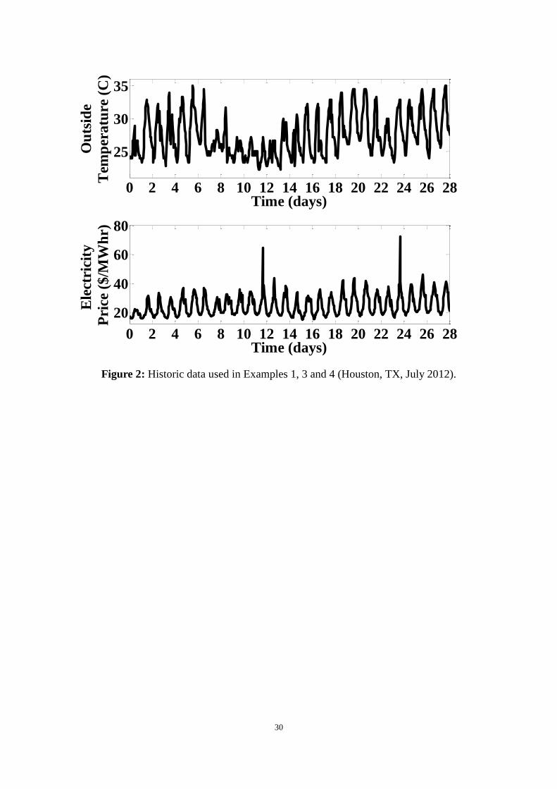
Example 1: This example uses the Full Future Information (FFI) scenario of [14]. This is the
case under which all future information is assumed to be known to the controller. This scenario
has been chosen to exemplify the impact of horizon size on EMPC performance without having
to wonder if the results obtained are due in part to forecasting issues. Outside temperature and
cost of electricity will be those indicated in Figure 2. The outside temperature corresponds to
historic hourly data from Houston, TX (July, 2012), [17], and the electricity prices correspond
to the historic real-time prices for the same period and location, [6].
The cost of operating the plant during period i is given as: , ,e i c i sC P t , where Pc,i is power
to the chiller, Ce,i is the price of electricity and ∆ts is the sample-time chosen to be one hour for
all examples presented in this work. Thus, an appropriate definition of the EMPC objective
function is |( ) 0N i N ig s and
| | | , | , |( , , )N k i k ei k i k i c k ig s m C Pp (6)
The EMPC simulations to follow were implemented with Mathworks MATLAB on an Intel
Pentium Dual CPU T3200 @ 2.00 GHz with 3.00 GB RAM. The simulation length was 28
days for all cases. As a baseline, the 24 hour horizon EMPC was implemented assuming zero
TES, and resulted in an operating cost of $827. Assuming the TES to be 1.5 TMW hr , resulted
in an operating cost (with the 24 hour EMPC) of $520 (a reduction of 37.1% compared to the
baseline) and required 13 s of computational time. The same simulation with a 2 hour EMPC
horizon resulted in an operating cost of $651 (a reduction of only 21.3%) and required 7 s. The

6
loss of economic performance is observed in Figure 3, which shows significant inventory creep
for the 2N case.
While the computational effort of the 24 hour horizon case of Example 1 seems sufficient for
on-line implementation, it is highlighted that the model is exceedingly simple with only 5 states.
In addition, the model does not account for internal equipment and occupant heating, nor does
it consider indoor air quality and humidity. Furthermore, if one would like to consider the
larger question of system design (the subject of part 3 in this series of papers), then fast
simulation times will be required to achieve computational tractability.
In the following section, a control policy alternative to EMPC will be developed. This policy
will have similar economic motives, but will be a linear feedback. In section 3, this Economic
Linear Optimal Control (ELOC) policy will be extended to account for point-wise-in-time
constraints.
2 ECONOMIC LINEAR OPTIMAL CONTROL (ELOC)
Before we begin the ELOC development it is important to emphasize that the goal is to develop
an approximation of the EMPC policy. Thus, we are free to explore other optimization
problems that are similar to problem (5), but clearly different. Of course, the level of similarity
will impact the quality of the approximation. As in [14] it will be convenient to distinguish the
process model (representing the physical structure) from the shaping filter model (representing
the disturbances). In the building HVAC case, the process model is of the following linear form
( ) ( ) ( ) ( ) ( ) ( )
1
p p p p p p
i d i d i d is A s B m G p (7)
( ) ( ) ( ) ( ) ( )p p p p p
i x i u iq D s D m (8)

7
where as in Section 1, ( )
0 11 12 21
Tp
ss T T T T E , ( ) Tp
s cm Q Q , ( )
3
Tp
ep T C .
The average of the state, manipulated and output variables must satisfy
( ) ( ) ( ) ( ) ( ) ( )p p p p p p
d d ds A s B m G p (9)
( ) ( ) ( ) ( ) ( )p p p p p
x uq D s D m (10)
Deviation variables can then be defined as ( ) ( ) ( )p p p
i ix s s , ( ) ( ) ( )p p p
i iu m m , ( )f
i iz p p
and ( )p
i iz q q , which results in the following model:
( ) ( ) ( ) ( ) ( ) ( ) ( )
1
p p p p p p f
i d i d i d ix A x B u G z (11)
( ) ( ) ( ) ( ) ( )p p p p p
i x i u iz D x D u (12)
The disturbance sequence, ip , is assumed to be a stochastic process and the output of the
following linear shaping filter.
( ) ( ) ( ) ( ) ( )
1
f f f p f
i d i d ix A x G w (13)
( ) ( ) ( )f f f
i x iz D x (14)
where ( )f
iw is a zero mean, white noise sequence with covariance ( )f
w and ( )f
i ip z p .
Combining the two models into a single compound system gives
( ) ( ) ( )
1
c c c
i d i d i d ix A x B u G w (15)
( ) ( )c c
i x i u iz D x D u (16)
where ( ) ( )T T T
p f
i i ix x x
, ( )p
i iu u , ( )f
i iw w , ( ) ( )T T T
p f
i i iz z z
and
( ) ( ) ( ) ( )
( ) ( ) ( )
( )( )
0, ,
0 0
p p f p
c c cd d x d
d d d ffdd
A G D BA B G
GA
(17)
( ) ( )
( ) ( )
( )
0,
0 0
p p
c cx u
x uf
x
D DD D
D
(18)
The sequence ip should not be confused with its associated forecasts | | 1|
ˆ ˆ, ,pk i k i k ip p .
The difference is that |pk i will be a function of the measurements and its characteristics will

8
be strongly influenced by the measurement structure. Consider the Zero Future Information
(ZFI) scenario of [14]. In this case, the forecasts, |pk i , will be a function of the estimate of the
filter state, ( )ˆ f
ix , which is a function of the current and past measurements. In the Pseudo
Future Information (PFI) case of [14], similar observations can be made, although in this case
the shaping filter (13)-(14) will need to be the compound PFI form discussed in [14]. In
contrast, ip is assumed to be the actual signal at time i . This is distinctly different from the
forecast |pk i . Thus, our first major modification to problem (5) is to assume that the feedback
policy is a function of measurements at time i . This modification is significant. As opposed to
problem (5), which would appropriately be characterized as generating an Open-Loop Optimal
Feedback (OLOF) policy, the optimal control problem to be proposed will produce a
Closed-Loop Optimal Feedback (CLOF) policy. (Strictly speaking, the feedback
implementation of EMPC makes it a function of measurements at time i . However, the
optimization problem it solves at each time step assumes perfect knowledge of the future even
if forecasts are employed. This open-loop based solution to the optimization problem is where
the distinction is made.)
Initially, assume the measurements are of a Full State Information (FSI) form, in that
i iy x . Thus, the feedback policy at time i can be a function of ix , which contains both the
process and shaping filter state at time i . Removal of this assumption, which will call for
i i iy Cx , results in the Partial State Information (PSI) framework. In this case, it will be a
simple matter to generalize from the FSI results and make the feedback policy a function of the
state estimate ˆix . It should be emphasized that the distinction between FSI vs PSI is unrelated
to the questions of ZFI vs PFI. Specifically, the latter is dictated by the form of the shaping

9
filter model, while the former depends on the values assumed for C and v . Of course, the
latter will influence the dimension of C and v .
The second major modification is to remove the inequality constraints min max
p p p
iq q q
and replace with constraints on the statistics of the closed-loop system. Concerning the first
order statistics, the mean of the output will be constrained as ( )(p) p (p)
min maxq q q where ( )pq
must also satisfy (9) - (10). Concerning second order statistics, let j denote the steady-state
standard deviation of the jth element of
( )p
iq . Then we will require
m i n ,
p p
j jjn q q (19)
max,
pp
j j jn q q (20)
where n is a parameter indicating the number of standard deviations the average, ( )p
jq , must
be from the bounds, max,
p
jq and min,
p
jq . The important aspect of these new constraints is that
j will be directly influenced by the feedback element. If this feedback is linear with respect
to the process and shaping filter states, i iu Lx (our third modification), then these
steady-state standard deviations [14] are calculated as
j j (21)
T
j j z j (22)
( ) ( ) ( ) ( )( ) ( )c c c c T
z x u x x uD D L D D L (23)
( ) ( ) ( ) ( ) ( ) ( )( ) ( )Tc c c c T c c
x d d x d d d w dA B L A B L G G (24)
where j is the j th row of identity with dimension equal to that of z .
The objective function for our ELOC problem is stated as
( ) ( )
0
1lim ( , ) lim ,
Np p
i i i iN i
i
g q p E g q pN
In the building HVAC system, ( )
, ,,p
i i c i e ig q p P C . Thus the objective function is

10
( )
, ,lim , limp
i i c i e i c ei i
E g q p E P C PC
where , ,c i c i cP P P and , ,e i e i eC C C . Since ,c iP and ,e iC are elements of iz the term
, ,limi c i e iE P C can be calculated as one of the off-diagonal elements of z . Similarly, cP
is an element of ( )pq and eC is an element of p . Thus, for appropriate definitions of 1a , 2a
and 0A the objective can be written as ( )
1 2 0
T T T p
za a p A q and the ELOC problem can be
stated as
( ) ( ) ( )
( )
1 2 0, , , 0, 0,
, 0, 0
min ( )
. . (9), (10), (19) (24)
p p pj i
z x
T T p
zs m q
L
a a A p q
s t
(25)
Unfortunately, a computationally tractable method of solving problem (25) could not be found.
As an alternative, we propose to enforce the following additional constraint
, 1 , 2 , 3 ,c i S i D i I iP C C C (26)
where ,S iC , ,D iC and ,I iC are all signals related to ,e iC and 1 , 2 , and 3 are scalar
parameters to be selected by the optimization. More specifically, ,S iC is the short-term
average of ,e iC , while , , ,D i e i S iC C C . Then, ,I iC is defined as the integral of ,D iC . Based on
these definitions it is appropriate to assume all three are orthogonal , , 0S i D iE C C ,
, , 0S i I iE C C and , , 0D i D iE C C . Thus, the covariance term of the objective function
may be reevaluated
, , 1 , 2 , 3 , , ,
2 2
1 , 2 ,
1 2
lim lim
lim
S D
c i e i S i D i I i S i D ii i
S i D ii
C C
E P C E C C C C C
E C E C
where SC and
DC are the known variances of sC and DC , respectively. Using this
objective function along with constraint (26), we were able to find a computationally tractable

11
solution for the ELOC problem. The details of this development can be found in Appendix 1.
It is highlighted that the use of ,I iC in equation (26) distinguishes the current ELOC
formulation from that of [18]. In essence, this term allows the resulting controller to devote
sufficient effort to the attenuation of process disturbances. It is additionally noted that the use
of a fourth term in equation (26) corresponding to the integral of ,S iC was also investigated.
However it was found that this term either had no impact or in some cases degraded
performance.
Example 2: Return to the scenario of Example 1 and replace the assumption of FFI with ZFI.
Furthermore, assume the disturbances are generated by the 4th order shaping of [14]. As such,
the internal states of the shaping filter will be available to the simulation and thus the FSI
feedback may be implemented.
The plots of Figure 4 clearly indicate that the ELOC policy has a tendency for smart grid
coordination in that heat to the chiller increases when prices are low and decreases when high.
In addition, regulation of room temperature is rather aggressive in that the variance of this
output is small so that the average of room temperature can be very close to its maximum of
25oC and cP will be minimized. This aligns with the characteristics of the EMPC trajectories
as well as the objective function of the ELOC, which includes e cC P . Where the ELOC policy
seems to fail is in the observance of constraints. However, a closer inspection indicates that it is
doing exactly as instructed, in that it is observing the statistical version of the constraints. The
next section will illustrate how point-wise-in-time constraints can be enforced.
Example 3: To implement the ELOC in the more realistic scenario of having only
measurements of the disturbance and not those of the internal states of the shaping filter, the

12
feedback will need to be a function of the state estimates ˆix , or ˆi iu Lx . Appendix 2 illustrates
how to extend the FSI formulation to the PSI case. Using the historic data of Figure 2 along
with measurement characteristics detailed in [14], and the 4th order filter of Example 2 for state
estimation, the plots of Figure 5 resulted. These plots indicate ELOC performance similar to
that of Figure 4. The main difference is in the energy storage plot where a substantial deviation
from the average seems to occur during days 5 and 6. This results because the 4th order shaping
filter within the state estimator is having a bit of trouble estimating the short-term average of
the historic data used in this example. This deviation along with all other constraint violation
will be removed next.
3 CONSTRAINED ELOC
Let us begin by taking stock of the previous section. Basically, we have identified a feedback
control policy (the ELOC policy) that is a linear function of the physical states of the process as
well as the internal states of the shaping filter: i ELOC iu L x . Using the building HVAC
example we have shown that application of the ELOC policy will result in a closed-loop
trajectory that is similar to that generated by the EMPC policy.
Development of the Constrained ELOC policy begins by converting the ELOC policy from
its linear feedback form to its predictive form. Once in the predictive form, one can simply
impose point-wise-in-time constraints to the predicted trajectories. Specifically, the predictive
form of the ELOC policy is defined as
| | |
1
| |, ,min ,
k i k i k i
i N
k i k i N i Nx u q
k i
x u x
(27)

13
( ) ( )
1| | |. . , 1, , 1c c
k i d k i d k is t x A x B u k i N (28)
|ˆ
i i ix x (29)
Where c
dA and c
dB are as defined in (17), ( ) T
N i N i N ELOC i Nx x P x and
| |
| |
| |
( , )
T
k i k iELOC ELOC
k i k i Tk i k iELOC ELOC
x xQ Mx u
u uM R
(30)
If one were to use the LQR inverse optimality results of [3] to generate weights ELOCQ , ELOCR ,
ELOCM and ELOCP that correspond to ELOCL , then the policy generated by (27) will be
identical to i ELOC iu L x . It is important to note that [21] guarantees that such weights can be
generated for all linear feedbacks produced from a class of problems to which the ELOC
problem is a member. As a convenience to the reader, the ELOC controller, ELOCL , of Example
3 along with its inverse optimal matrices ELOCQ , ELOCR , ELOCM and ELOCP are given in
Appendix 3.
Then, the Constrained ELOC policy is simply problem (27) augmented by the following
point-wise-in-time constraints
| | |k i x k i u k iz D x D u (31)
( ) ( ) ( ) ( )
min | max
p p p p
k iq q z q q (32)
Example 4: Reconsider the scenario of Example 3. The plots of Figure 6 compare the EMPC
with the Constrained ELOC (both using ZFI, PSI and a horizon of 24 hours). Clearly, the
point-wise-in-time constraints are now being enforced by the Constrained ELOC and the plots
indicate a qualitative similarity to the EMPC policy. Quantitatively, the Constrained ELOC
policy has an expenditure of $567 over 28 days, and actually outperforms the EMPC policy
with expenditures of $575.
The important feature of the Constrained ELOC policy is its virtual insensitivity with respect

14
to horizon size, N . Figure 7 compares the Constrained ELOC policy using horizons of 24 and
2 hours. Clearly, the two are remarkably similar. The expenditures using a 2 hours horizon are
$552 over 28 days. The computational benefits of Constrained ELOC are also highlighted in
Table 1.
The source of this horizon insensitivity stems from the fact that forecasting capabilities of
the shaping filter are incorporated into the ELOC policy and through inverse optimality
translated into the Constrained ELOC objective function weights, most notably PELOC. This
final cost term represents the forecasted trajectory from the end of the horizon to infinity. Thus,
a change in horizon size does not change the forecasts. It only changes point-wise-in-time
constraint enforcement on the forecasted trajectory. This is in stark contrast with the EMPC
policy, where the forecast after the horizon is abruptly changed to zero.
It is interesting to note that in problem (27) a portion of the predicted state, |k ix , 1, ,k N
can be pre-specified. This is due to the fact that the shaping filter state cannot be influenced by
the manipulated variable. Thus, the only way the optimization can satisfy the shaping filter
portion of (28) is to set the shaping filter states equal to those that would be generated by the
forecasts. Said more compactly, *( ) ( )
| |ˆf f
k i k ix x . Thus, a reduction in computational effort can be
achieved by setting the shaping filter variables equal to the forecasts, which would remove the
shaping filter associated equations from (28). While this observation did improve
computational efficiency for the ZFI case (reported in Table 1), it will likely be essential for the
PFI case where the state of the shaping filter will be much larger.

15
4 CONCLUSIONS
In this work we have shown that the performance of EMPC in a building HVAC application
is significantly influenced by the choice of horizon size, i.e., while short horizons will yield a
computational advantage, they can also result in significant degradations in expenditure
savings. A major contribution of the current effort was to show that a linear feedback policy
(the ELOC policy) can be constructed to yield closed-loop trajectories very much similar to
those of large horizon EMPC. This ELOC Policy is distinct from that of [18] in that it can also
respond to process level disturbances and not just utility cost disturbances. Then, an extension
of ELOC to the Constrained ELOC policy will yield a controller that again has characteristics
similar to EMPC, but also enforces point-wise-in-time constraints. In fact, under the
assumption of ZFI and a PSI structure, the Constrained ELOC outperforms the large horizon
EMPC. The critical feature of this Constrained ELOC policy is its virtual insensitivity to
horizon size. Thus, application of the Constrained ELOC policy with a short horizon was able
to yield the best of both worlds: a reduction in computational effort while preserving (or
improving) economic performance.
It is highlighted that the methodology presented can be applied to other scenarios through
simple modification Equations (17) and (18). Specifically, the user would provide a building
model, which in practice can be obtained through first principles modeling or through a data
driven model scheme (i.e., system identification based on building response data). As for the
disturbance model, the statistical parameters (mean and variance) for the electricity prices and
weather conditions could be modified within the model used in this work (and presented in
[14]), or again a data driven modeling scheme could be employed. It is also noted that for a

16
given building one may want to update the Constrained ELOC policy in response to seasonal
changes in the electricity and weather characteristics. Specifically, one could re-run the ELOC
problem using seasonally appropriate values for the mean and variance of these signals.
Similarly, one could update the value for chiller efficiency c based on a change in the average of
outside temperature, which would likely result in a more appropriate ELOC policy. If one
would like to make chiller efficiency a true function of outside temperature, then the linearity
of the building model would be invalidated. However, as highlighted in [20], a linear dynamic
model is only required to determine the Constrained ELOC objective function weights. Once
these weights have been determined, the predictive model in (27) can be replaced with a
nonlinear model within the on-line optimization of the Constrained ELOC policy, assuming an
appropriate and sufficiently fast nonlinear solver is used for on-line implementation.
ACKNOWLEDGMENTS
Both authors would like to thank the National Science Foundation (CBET-0967906) for
financial support.
REFERENCES
[1] R. Amrit, J. B. Rawlings, and D. Angeli, "Economic Optimization using Model Predictive
Control with a Terminal Cost," Annual Reviews in Control, vol. 35, pp. 178-186, 2011.
[2] D. Angeli, R. Amrit, and J. B. Rawlings, "On Average Performance and Stability of
Economic Model Predictive Control," IEEE Trans. Aut. Contr., vol. 57, no. 7, pp.
1615-1626, 2012.
[3] D. J. Chmielewski and A. M. Manthanwar, "On the Tuning of Predictive Controllers:
Inverse Optimality and the Minimum Variance Covariance Constrained Control
Problem," Ind. Eng. Chem. Res., vol. 43, pp. 7807-7814, 2004.

17
[4] M. Diehl, R. Amrit, and J. B. Rawlings, "A Lyapunov Function Economic Optimizing
Model Predictive Control," IEEE Trans. Aut. Contr., vol. 56, no. 3, pp. 703-707, 2011.
[5] M. Ellis, H. Durand, and P. D. Christofides, "A Tutorial Review of Economic Model
Predictive Control Methods," J. Proc. Contr., vol. 24, pp. 1156-1178, 2014.
[6] Ercot. (2012) Historic Real Time Data Electricity Prices for Houston Texas. [Online].
http://www.ercot.com/mktinfo/prices/
[7] L. Grune, "Economic Receding Horizon Control Without Terminal Constraints,"
Automatica, vol. 49, pp. 725-734, 2013.
[8] M. Heidarinejad, J. Liu, and P. D. Christofides, "Economic Model Predictive Control of
Nonlinear Process Systems using Lyapunov Techniques," AIChE J., vol. 58, pp. 855-870,
2012.
[9] R. Huang, L. T. Biegler, and E. Harinath, "Robust Stability of Economically Oriented
Infinite Horizon NMPC that Include Cyclic Processes," J. Proc. Contr., vol. 22, no. 1, pp.
51-59, 2012.
[10] R. M. Lima, I. E. Grossmann, and Y. Jiao, "Long-Term Scheduling of a Single-Unit
Multi-Product Continuous Process to Manufacture High Performance Glass," Computers
& Chemical Engineering, vol. 35, pp. 554-574, 2011.
[11] D. I. Mendoza-Serrano, Smart Grid Coordination in Building HVAC Systems. Chicago:
PhD Thesis, Illinois Institute of Technology, 2013.
[12] D. I. Mendoza-Serrano and D. J. Chmielewski, "Controller and System Design for HVAC
with TES," in Proc. of the Am. Cont. Conf., Montreal, Canada, 2012.
[13] D. I. Mendoza-Serrano and D. J. Chmielewski, "HVAC Control Using Infinite-Horizon
Economic MPC," in Proc. of the 51st IEEE Conference on Decision and Control, Hawaii,
USA, 2012.
[14] David I Mendoza-Serrano and Donald J Chmielewski, "Smart Grid Coordination in
Building HVAC Systems: EMPC and the Impact of Forecasting," J. Proc. Contr., vol. 24,
no. 8, pp. 1301-1310, 2014.
[15] M.A. Muller, D. Angeli, and F. Allgower, "Economic Model Predictive Control with
Self-Tuning Terminal Cost," European Journal of Control, vol. 19, no. 5, pp. 408-416,
2014.
[16] M.A. Muller, D. Angeli, and F. Allgower, "On Convergence of Averagely Constrained
Economic MPC and Necessity of Dissipativity for Optimal Steady-State Operation," in
Proc. of the Am. Cont. Conf., 2013, pp. 3147-3152.
[17] (NCDC) National Climatic Data Center. (2012) Hourly Climate Data for Houston Texas.
[Online]. http://www.ncdc.noaa.gov/oa/climate/climatedata.html
[18] B. P. Omell and D. J. Chmielewski, "IGCC Power Plant Dispatch Using Infinite-Horizon
Economic Model Predictive Control," Ind. Eng. Chem. Res., vol. 52, no. 9, pp. 3151-3164,
2013.
[19] B. P. Omell and D. J. Chmielewski, "On the Stability of Infinite Horizon Economic MPC,"
AIChE Annual Meeting, 2013.
[20] B. P. Omell and D. J. Chmielewski, "On the Tuning of Predictive Controllers: Impact of

18
Disturbances, Constraints, and Feedback Structure," AIChE J., vol. 60, no. 10, pp.
3473-3489, 2014.
[21] J. K. Peng, A. M. Manthanwar, and D. J. Chmielewski, "On the Tuning of Predictive
Controllers: The Minimally Backed-off Operating Point Selection Problem," Ind. Eng.
Chem. Res., vol. 44, pp. 7814-7822, 2005.
[22] J. B. Rawlings, D. Angeli, and C. N. Bates, "Fundamentals of Economic Model Predictive
Control," in Proc. of the 51st IEEE Conference on Decision and Control, Hawaii, USA,
2012.
[23] J. B. Rawlings, D. Bonne, J. B. Jorgensen, A. N. Venkat, and S. B. Jorgensen,
"Unreachable Setpoints in Model Predictive Control," IEEE Trans. Aut. Contr., vol. 53,
no. 9, pp. 2209-2215, 2008.
[24] L. Wurth, I. J. Wolf, and W. Marquardt, "On the Numerical Solution of Discounted
Economic NMPC on Infinite Horizons," in Preprints of the 10th IFAC International
Symposium on Dynamics and Control of Process Systems, 2013, pp. 209-214.
APPENDIX 1
A computationally tractable approach to solving the ELOC problem begins by redefining the
shaping filter,( ) ( ) ( ) ( ) ( )
1
f f f f f
i d i d ix A x G w ,( ) ( ) ( )f f f
i x iz D x , such that
iSiIiDiS
f
i CCCCz ,,,,
)( ~~~~ , In the 4th order shaping filter of [14], these outputs arise
naturally from the constructed states. If a system identification procedure has been used to
construct the shaping filter from historic data, then see [11] for an appropriate procedure.
To address the bilinearity associated with 1 ,S iC , recognize that 1 , ,S i S iC C , where ,S iC
is determined as the output of the following filter
( ) ( ) ( ) ( ) ( )
1 1
f f f f f
i d i d ix A x G w
( ) ( )
, 1
f f
S i x iC D x
Similar relations for the other bilinear terms can be achieved through the following compound
shaping filter
( ) ( ) ( ) ( ) ( )
1
fc fc fc fc fc
i d i d ix A x G w (33)

19
( ) ( ) ( )fc fc fc
i x iz D x (34)
where
31 2 4
31 2 4
1
2
3
( )( ) ( ) ( )( )
( )
, , , 3,
( ) ( ) ( ) ( ) ( )
( )( ) ( ) ( )( )
1 2 3
( ) ( )
( ) ( )
( )
0 0 0
0 0 0
0 0
TT T T
T
T
Tff f ffc
i i i i i
Tfc
i S i D i I i i
fc f f f f
d d d d d
ff f ffc
d d d d d
Tf f
d d
Tf f
d d
f
d
x x x x x
z C C C T
A diag A A A A
G G G G G
G G
G G
G
4
( )
( ) ( )
( )
1
( )
( ) 2
( )
3
( )
4
0
0 0 0
0 0 0
0 0 0
0 0 0
0 0 0
T
T
Tf
d
Tf f
d d
f
x
f
fc x
x f
x
f
x
G
G G
D
DD
D
D
Recall that j is the jth row of identity ( 4 4I in this case). The idea being that since each
( )jf
ix signal, 1, 2, 3j , is driven by the same white noise sequence, ( )f
iw , each will be
identical to 4( )f
ix , with the exception of being scaled with respect to j . Then, the process and
shaping filter model can be redefined as
( ) ( ) ( )
1
e e e
i d i d i d ix A x B u G w (35)
( ) ( )e e
i x i u iz D x D u (36)
where ( ) ( )T T T
p fc
i i ix x x
, ( ) (0)T T T
p
i i iz z z
, ( )f
i iw w , ( )p
i iu u ,
( ) ( ) ( )
( )
( )0
p p fc
e d d x
d fc
d
A G DA
A
, ( )
( )
0
p
e d
d
BB
, ( )
( )
0e
d fc
d
GG
,
( )
( )
3 ( )
1
0
0
p
xe
x fc
j j x
DD
D
,
( )
( )
p
e u
u
DD

20
4
1 2
, 0 c and
(0)
iz is defined as , , , ,C i S i D i I iP C C C . Using (35) - (36)
the ELOC problem can be defined as
( ) ( ) ( )
1 2 3
( )
1 2 0, , , , , ,
0, 0, , 0
min ( )S Dp p p
j j x
T p
C Cs m q
L
A p q
(37)
( ) ( ) ( ) ( ) ( ) ( ). . p p p p p p
d d ds t s A s B m G p (38)
( ) ( ) ( ) ( ) ( )p p p p p
x uq D s D m (39)
( )
min,
( ) 1, ,p
j j j q
pn q q j n (40)
( )
max,
( ) 1, ,p
j j j q
pn q q j n (41)
2 1, ,j j qj n (42)
( ) ( ) ( ) ( ) ( ) ( )TTe e e e e e
x d d x d d d w dA B L A B L G G (43)
( ) ( ) ( ) ( ) 1, , 1T
e e e e T
j j x u x x u j qD D L D D L j n (44)
1qn (45)
The last constraint 1qn is enforcing the condition (0) 2lim ( )i iE z , and is
essentially requiring ,c iP ≃ 1 , 2 , 3 ,S i D i I iC C C . The only computational challenges
associated with problem (37) concern the reverse convexity of (42) and the non-linearity of (43)
- (44). However, the following Theorem (a simple extension of that found in [3]) will exactly
convert (43) - (44) to convex constraints.
Theorem A1: There exists 0x , stabilizing L , and 0j , 1, , 1qj n such
that
( ) ( ) ( ) ( ) ( ) ( )TTe e e e e e
x d d x d d d w dA B L A B L G G (46)
( ) ( ) ( ) ( ) 1, , 1T
e e e e T
j j x u x x u j qD D L D D L j n (47)
2 1, , 1j j qz j n (48)

21
if and only if there exists 0X , Y , and 0j , 1, , 1qj n such that
( ) ( ) ( )
( ) ( )
( ) 1
0 0
0T
e e e
d d d
Te e
d d
e
d w
X A X B Y G
A X B Y X
G
(49)
( ) ( )
( ) ( )0, 1, , 1
e e
j j x u
qTe e T
x u j
D X D Yj n
D X D Y X
(50)
2and 1, , 1j j qz j n (51)
Using Theorem A1, the ELOC problem can be re-stated as:
( ) ( ) ( )
1 2 3
( )
1 2 0
0, , 0, 0, , , , , ,
min ( )
. . (38) (42), (45), (49), (50)
S D
j z j
p p p
T p
C C
X Ys m q
A p q
s t
(52)
It should be emphasized that the linearity of ( )e
dG with respect to 1 , 2 and 3 guarantees
that constraint (49) is a Linear Matrix Inequality (LMI). Finally, the non-convex constraints of
(42), are addressed using the branch and bound procedure detailed in [21]. Use of this branch
and bound algorithm to solve (52) guarantees that the found solution is the globally optimal
solution.
The solution to problem (52) will generate a set of optimal matrices * 0X and *Y . From
these, a feasible feedback is calculated as * * * 1
( ) ( )eL Y X . Due to the expansion of the shaping
filter model (to account for the j parameters) this feedback gain will be of the following
form
1 2 3 4
* * * * * *
( ) ( ) ( ) ( ) ( ) ( )e p f f f fL L L L L L (53)
since problem (52) believes this gain will be a linear feedback of the state ( ) ( )T T T
p fc
i ix x
. To

22
be an appropriate feedback for the original system, equations (15) - (16), the gain should be
computed as
4
3* * * * * *
( ) ( ) ( ) ( ) ( )
1
wherejELOC p f f f j f
j
L L L L L L
(54)
And the *
j s are the optimal values from problem (52).
APPENDIX 2
In the PSI case, the compound system analogous to (15) – (16) is
( ) ( ) ( )
1
c c c
i d i d i d ix A x B u G w (55)
( ) ( )c c
i x i u iz D x D u (56)
( )c
i i iy C x v (57)
where ( ) ( )T T T
p f
i i ix x x
, ( )p
i iu u , ( ) ( )T
p f
i i iw w w ,
( ) ( )T T Tp f
i i iz z z
,
( ) ( ) ( ) ( 2)( )
( ) ( ) ( )
( ) ( )
0, ,
0 00
p p f pp
c c cd d x dd
d d df f
d d
A G D GBA B G
A G
( ) ( ) ( )
( ) ( ) ( )
( ) ( )
0 0, ,
0 0 0
p p p
c c cx u
x uf f
x
D D CD D C
D C
( ) ( )
( ) ( )
( ) ( )
0 0,
0 0
p p
c cw v
w vf f
w v
( 2) ( 2)p p
d sG t G , ( 2) 0 0 0 0 1TpG , ( ) ( ) /p p
w w sS t , ( ) 1p
wS , ( ) ( )f f
xC D ,
( )
1 5
Tp T TC
, ( ) /p
v sI t , ( ) 23 /f
v sI t . Using (59) and (57) the following optimal
state estimator can be constructed
( ) ( ) ( ) ( )
1 1ˆ ˆc c c c
i d i d i ix A x B u K (58)
where ( ) ( ) ( )
1 1ˆc c c
i i d i d iy C A x B u , 1
( ) ( ) ( ) ( ) ( )T Tc c c c c
vK HC C HC
, where H is
the positive definite solution to

23
1
( ) ( ) ( ) ( ) ( ) ( ) ( ) ( ) ( )T T T Tc c c c c c c c c
d v d d w dH A H HC C HC C H A G G
A convenient feature of the optimal state estimator is that the innovation sequence, i , is
white noise with a covariance ( ) ( ) ( ) ( )Tc c c c
vC HC . Thus, equation (58) can be used as
the starting point for the convex formulation of the PSI version of ELOC (just as (15) was
the starting point for the FSI case). The point to recognize is that the Kalman gain, ( )cK ,
should be partitioned into two blocks: process rows and shaping filter rows
( )
( )
( )
p
c
f
KK
K
Then, the PSI process, analogous to (35) - (36), is defined as
( ) ( ) ( ) ( )
1 1ˆ ˆe e e c
i d i d i ix A x B u K (59)
( ) ( ) ( ) ( )ˆe e e p
i x i u i x iz D x D u D x (60)
where ( )e
dA , ( )e
dB , ( )e
xD and ( )e
uD are unchanged and
31 2 4
1
2
3
4
( )
( )
( )
( )( ) ( ) ( )( )
1 2 3
( ) ( )
( ) ( )
( ) ( )
( ) ( )
( )
( )
0 0 0
0 0 0
0 0 0
0 0 0
0
0 0
T
T
T
T
p
e
fc
ff f ffc
Tf f
Tf f
Tf f
Tf f
p
e x
x
KK
K
K K K K K
K K
K K
K K
K K
DD
( ) ( ) ( )ˆp p p
i i ix x x and has a covariance of ( )pp
x from
( ) ( )
1( ) ( ) ( ) ( ) ( ) ( )
( ) ( )
T T
T
pp pf
x xc c c c c c
x vpf ff
x x
HC C HC C H
Then, if ˆi iu Lx and the fact that ˆ 0T
i iE x x is employed, one finds the following

24
covariance relations
( ) ( ) ( ) ( ) ( ) ( ) ( )
ˆ ˆ
( ) ( ) ( ) ( ) ( ) ( ) ( )
ˆ
T
T
Te e e e e c e
x d d x d d
Te e e e p pp p T
j j x u x x u x x x j
A B L A B L K K
D D L D D L D D
Re-application of Theorem A1 results in the following LMI constraints
( ) ( ) ( )
( ) ( )
1( ) ( )
0 0
0T
e e e
d d
Te e
d d
e c
X A X B Y K
A X B Y X
K
(61)
( ) ( ) ( ) ( ) ( )
( ) ( )0, 1, , 1
Tp pp p T e e
j j x x x j j x u
qTe e T
x u j
D D D X D Yj n
D X D Y X
(62)
Re-evaluation of the objective function with
, 1 , 2 , 3 ,
ˆ ˆ ˆc i S i D i I iP C C C (63)
yields
2
, , 1 , , ,
2
2 , , ,
3 , , , ,
1 1 2 2 3 3
ˆ ˆ ˆ ˆlim lim{
ˆ ˆ ˆ
ˆ ˆ ˆ ˆ}
c i e i S i S i D ii i
D i S i D i
I i S i I i D i
E P C E C E C C
E C C E C
E C C E C C
d d d
with ( ) ( )
ˆ ˆ1 1 1 1 2
f T f T
z zd , ( ) ( )
ˆ ˆ2 2 1 2 2
f T f T
z zd and
( ) ( )
ˆ ˆ3 3 1 3 2
f T f T
z zd where ( ) ( ) ( ) ( )
ˆˆ
Tf f f f
z x x xD D , ( ) ( ) ( )
ˆ
f f f
x x x ,
( ) ( ) ( ) ( ) ( ) ( ) ( )T Tf f f f f f f
x d x d d w dA A G G and ( ) ( )f ff
x x .
Finally, the PSI version of the ELOC problem is stated as

25
( ) ( ) ( )
1 2 3
( )
1 1 2 2 3 3 0
0, , 0, 0, , , , , ,
min ( )
. . (38) (42), (45), (61), (62)
j z j
p p p
T p
X Ys m q
d d d A p q
s t
(64)
APPENDIX 3
For Example 3, 1 2 3 4 5
* * * * * * *
( ) ( ) ( ) ( ) ( ) ( ) ( )e p f f f f fL L L L L L L where
*
( )
0 0.0023 0.0012 0 -0.0003
0 0 0 0 0.0001pL
1
*
( )
0 0 -3.2486 0 0
0 0 3.3089 0 0fL
2
*
( )
0.0130 -0.0009 0 0 0
-0.0037 0.0003 0 0 0fL
3
*
( )
0.3350 -0.0230 0 -3.2452 0
-0.0968 0.0066 0 3.3079 0fL
4
*
( )
1.3665 -0.0936 20.2018 -14.2702 0
-0.3947 0.0270 0.1468 -0.1080 0fL
and* 2
1 7.8463 / $MW hr ,* 2
2 4.6828 / $MW hr and * 2
3 8.7867 / $MW hr .
Thus
0 0.0023 0.0012 0 -0.0003 30.1635 -1.6378 0.1123 -5.2878 14.2443
0 0 0 0 0.0001 -15.5833 0.4731 -0.0324 26.1091 -29.1734ELOCL
(65)
2Theorem A (from [3]): If there exists 0P and R such that
( ) *0
( )
T T T
d d d d
T T
d d d d
P A PA L R B PB L
R B PB L B PA R
then Q≜ ( )T T T
d d d dP A PA L R B PB L and M ≜ ( )T T
d d d dR B PB L B PA will be such
that

26
0T
Q M
M R
And P and L will satisfy
10 ( )( ) ( )T T T T T
d d d d d d d dA PA Q M A PB R B PB M A PB ,
1( ) ( )T T T
d d d dL R B PB M A PB .
Using Theorem A2, the following weights can be generated and will produce the
predictive form of the ELOC policy of (65)
11.8961 7.2991
7.2991 8.0397ELOCR
11 12
21 22
ELOC ELOC
ELOC
ELOC ELOC
P PP
P P
11
3.2565 -68.7075 65.9624 -0.3132 -0.0047
-68.7075 1548.3539 -1486.6413 7.1538 0.0008
65.9624 -1486.6413 1427.4137 -6.8665 -0.0013
-0.3132 7.1538 -6.8665 0.0338 -0.0002
-0.0047 0.0008 -0.0013 -0.0002 0.0002
ELOCP
12
-9.8391 -20.2813 2.2380 -6.9726 -0.2504
3.0372 1.3234 0.5126 3.2002 -1.1395
-2.5596 -7.5819 -0.4312 -1.7037 -0.0803
-0.9219 -0.7353 0.0520 -0.8986 0.5106
0.2495 1.0394 -0.0820 0.1111 0.1262
ELOCP
22
2624.0892 1198.4331 -101.7759 1652.0396 -848.8626
1198.4331 26534.3315 -1618.2108 -487.6575 3109.4071
-101.7759 -1618.2108 3336.7543 -37.4149 -173.5993
1652.0396 -487.6575 -37.4149 13902.7978 -1270.7266
-848.8626
ELOCP
3109.4071 -173.5993 -1270.7266 1512.2086
where 21 12T
ELOC ELOCP P . ELOCQ and ELOCM result from the algebraic relations of Theorem
A2. It should be noted that these weights are not unique and will likely vary depending on

27
the type and version of LMI solver used. The important point is that use of ELOCQ , ELOCR ,
ELOCM within the LQR problem will generate ELOCP and ELOCL .

28
Table 1: Comparison of EMPC and Constrained ELOC with 1.5 TMW hr of TES capacity for
28 days simulation historic data of Figure 2.
Controller Expenditure Percent
Reduction
Computational
Effort (s)
EMPC (FFI) with No TES $827 --- 13
EMPC (FFI) N = 24 hrs $520 37.1% 13
EMPC (ZFI PSI) N = 24 hrs $575 30.5% 13
EMPC (ZFI PSI) N = 2 hrs $673 18.6% 7
Constrained ELOC (ZFI PSI) N = 24 hrs $567 31.4% 13
Constrained ELOC (ZFI PSI) N = 2 hrs $552 33.3% 7

29
QcQr
Qs
Building
Thermal
Energy Storage
T3 PeChiller
Figure 1: Left: Process diagram for HVAC system with TES. Right: Description of building
zones.
Outside
Environment
(T3)
...
Windows
...
Walls
To T3T21T12 T11T11To To
...
Outside
Environment
(T3)
Room
Room
Room
Room
Room
Room
30
Figure 2: Historic data used in Examples 1, 3 and 4 (Houston, TX, July 2012).
0 2 4 6 8 10 12 14 16 18 20 22 24 26 28
25
30
35
Time (days)
Ou
tsid
e
Tem
per
atu
re (
C)
0 2 4 6 8 10 12 14 16 18 20 22 24 26 28
20
40
60
80
Time (days)
Ele
ctri
city
Pri
ce (
$/M
Wh
r)

31
Figure 3: Example 1 comparison of EMPC with a 24 hour horizon (solid line) and EMPC
with a 2 hour horizon. Both are FFI.
3 4 5 6
10
20
30
40
Time (days)
Ele
ctr
icit
y
O
uts
ide
P
ric
e
Tem
pera
ture
(
$/M
Wh
r)
(°
C)
3 4 5 6
0
200
400
Time (days)
Hea
t to
C
hil
ler
(kW
T)
3 4 5 6
-1500
-1000
-500
0
Time (days)
En
ergy i
n
Sto
rage
(kW
T h
r)

32
Figure 4: Example 2 comparison of FSI ELOC and FSI EMPC (24 hour horizon). Both are ZFI
and use a 4th order forecasting model.
3 4 5 6
10
20
30
40
Time (days)
E
lect
rici
ty O
uts
ide
P
rice
T
emp
eratu
re
($/M
Wh
r) (
°C)
T3
Ce
3 4 5 6-400
0
400
800
Time (days)
Hea
t to
C
hil
ler
(kW
T)
ELOC EMPC
3 4 5 6
-2000
0
2000
Time (days)
En
ergy i
n
Sto
rage
(kW
hr T
)
ELOC EMPC
3 4 5 622
24
26
Time (days)
Tem
per
atu
re
in R
oom
(°C
)
ELOC EMPC

33
Figure 5: Example 3 comparison of PSI ELOC and PSI EMPC (24 hour horizon). Both are ZFI
and use a 4th order forecasting model.
3 4 5 6
10
20
30
40
Time (days)
Ele
ctr
icit
y
O
uts
ide
P
ric
e
Tem
pera
ture
(
$/M
Wh
r)
(°
C)
T3
Ce
3 4 5 6
-400
0
400
Time (days)
Hea
t to
C
hil
ler
(kW
T)
ELOC EMPC
3 4 5 6
-4000
-2000
0
Time (days)
En
ergy i
n
Sto
rage
(kW
hr T
)
ELOC EMPC
3 4 5 622
24
26
Time (days)
Tem
per
atu
re
in R
oo
m (
°C)
ELOC EMPC

34
Figure 6: Example 4 comparison of Constrained ELOC and EMPC. Both are PSI/ZFI and with
horizons of 24 hours.
3 4 5 6
0
400
Time (days)
Hea
t to
C
hil
ler
(kW
T)
CELOC EMPC
3 4 5 6
-1500
-1000
-500
0
500
Time (days)
En
ergy
in
S
tora
ge
(kW
hr T
)
CELOC EMPC
3 4 5 622
24
26
Time (days)
Tem
per
atu
re
in R
oom
(°C
)
CELOC EMPC

35
Figure 7: Example 4 comparison of horizon size for Constrained ELOC with PSI/ZFI.
Solid - 24 hour horizon. Dashed - 2 hour horizon.
3 4 5 6
0
400
Time (days)
Hea
t to
C
hil
ler
(kW
T)
CELOC, N=2 CELOC, N=24
3 4 5 6
-1500
-1000
-500
0
500
Time (days)
En
erg
y i
n
Sto
rag
e (k
Wh
r T)
CELOC, N=2 CELOC, N=24
3 4 5 622
24
26
Time (days)
Tem
per
atu
re
in R
oo
m (
°C)
CELOC, N=2 CELOC, N=24