Smart Base Station Antenna Performance for Cellular Radio ... · PDF fileSmart Base Station Antenna Performance for Cellular Radio System ... based on uplink-downlink duality that

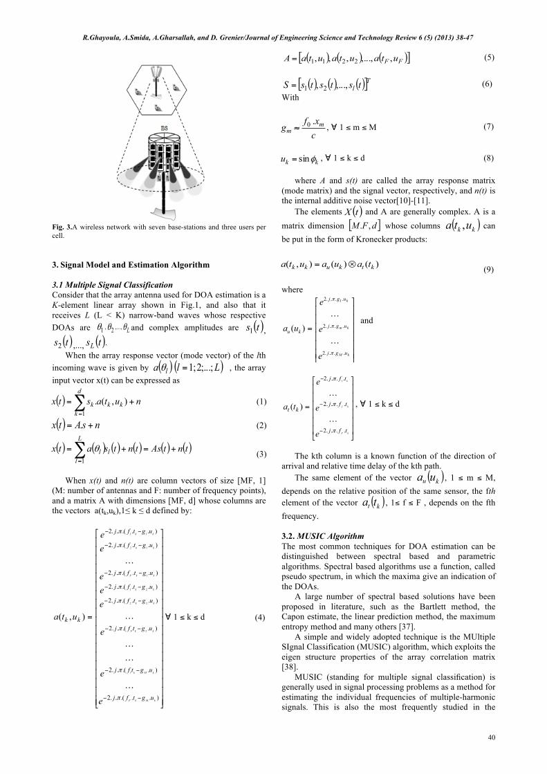
Journal of Engineering Science and Technology Review 6 (5) (2013) 38-47

Research Article

Smart Base Station Antenna Performance for Cellular Radio System

R.Ghayoula*,1,2, A.Smida1, A.Gharsallah1 and D. Grenier2

1 Unit of Research in High Frequency Electronic Circuits and Systems, Faculty of Mathematical, Physical and,Natural Sciences of Tunis, Tunis El Manar University, Campus Universitaire Tunis - El Manar – 2092, Tunis, Tunisia

2Department of Electrical and Computer Engineering, Laval University 1065, Avenue de la Médecine, Québec (QC), Canada, G1V 0A6

Received 17 April 2013; Accepted 25 December 2013 ___________________________________________________________________________________________ Abstract Adaptive array antenna technology is useful for detecting the Direction of Arrival (DOA) of signal and delay for mobile communications, where the antenna beam will automatically directed to the signal source. One method to estimate DOA and delay effectively is by using MUSIC (Multiple Signal Classification) algorithm. When the signal arrive at the antenna, the MUSIC algorithm will arrange the signal into its matrix covariance, and then perform an eigen decomposition process to produce the signal and noise subspace, and then obtain the power spectrum and delay spectrum. This paper combined the Taguchi method and MUSIC algorithm, used them as the prediction tool in designing parameters for the communication system and then constructed a set of the optimal parameter analysis flow and steps. Several adaptive beamforming criteria were discussed and a general form for the optimum array weight vector was derived that would require large amounts of computational load. Hence, it is necessary to find technique that can find optimum solution in real time. This paper will discuss the application of MUSIC algorithm for linear and circular array antenna in order to estimate the DOA and delay of various angles of elevation and azimuth.

Keywords: Taguchi, phased antenna array, Steering beams, MUSIC, TDOA,DOA, Interference nulling. ______________________________________________________________________________________ 1. Introduction ABASE transceiver station (BTS) is a piece of equipment that facilitates wireless communication between user equipment (UE) and a network. UEs are devices like mobile phones ,WLL phones, computers with wireless internet connectivity, WiFi and WiMAX devices and others. The network can be that of any of the wireless communication technologies like GSM, CDMA, Wireless local loop, WAN, WiFi, WiMAX, etc.

With the advent of mobile high-speed data applications, it is expected that the downlink of 3G CDMA systems will be the limiting link as far as capacity is concerned. Hence, it is important to investigate methods that can increase the downlink capacity to cope with increasing demand.

In cellular systems such as GSM or IS-95, antenna arrays can be used at base stations (BSs) to increase user capacity and provide other advantages such as improving voice quality, extending battery life in handsets and increasing data transmission rates. Array antennas have been employed in military systems for many years as a counter measure for deliberate, high power jammers [1].

Smart antenna systems are employed to overcome multipath fading, extend range, and increase capacity by using diversity or beamforming techniques in wireless communication systems [2]. Understanding of the smart base antenna performance mechanisms for various

environments is important design cost effective systems and networks. This dissertation focuses on the experimental characterization and modelling of the smart base station antenna performance for various propagation environment scenarios. In [3] the author’s describes a mobile communication base station antenna using a genetic algorithm based Fabry-Pérot resonance optimization. Their focal contribution is a beamformer-power update algorithm based on uplink-downlink duality that converges to a feasible solution to the problem. In the single-cell multi-user downlink case, the optimality of their algorithm was later proved by Visotsky and Madhow[4] and Schubert and Boche[5], [6].Recently, Wiesel, Eldar and Shamai[7] showed that the single cell downlink beamforming problem can be formulated as a second-order cone-programming problem. In [8] the author’s describes the smart antenna along with spatial diversity using fuzzy interference system and neural network (NN). In order to provide training for NN and fuzzy logic, a huge personalised training dataset is generated using Genetic Algorithm.

In this paper, a global optimization technique based on Taguchi method and MUSIC (Multiple Signal Classification) algorithm are applied so as to determine the excitation coefficients and the resultant pattern for a broadside discrete element array whose array factor will directly approximate the symmetrical sectoral pattern in order to estimate the DOA and delay of various angles of elevation and azimuth. The implementation system is described in detail, and linear antenna array examples are discussed to demonstrate its validity. Optimized results show

Jestρ

JOURNAL OF

Engineering Science and Technology Review

www.jestr.org

______________ * E-mail address: [email protected] ISSN: 1791-2377 © 2013 Kavala Institute of Technology. All rights reserved.

R.Ghayoula, A.Smida, A.Gharsallah, and D. Grenier/Journal of Engineering Science and Technology Review 6 (5) (2013) 38-47

39

that the desired array factors, a null controlled pattern and a sector beam pattern, are effectively obtained. It is found that neural network is an excellent candidate for optimizing diverse applications, as it is easy to realize and converges to the desired patterns rapidly. The paper is organized as follows. The synthesis problem formulation using Taguchi method is presented in section II. Multilayer Networks and Back-Propagation Algorithm is developed in section III. Section IV shows the novel design of phased antenna array with the simulation and measurement result, finally, section V makes conclusions. 2. Statement of Problem Adaptive array systems can locate and track signals (users and interferences) and dynamically adjust the antenna pattern to enhance reception while minimizing interference using signal-processing algorithms. A functional block diagram of such a system is shown in Fig 1 and Fig 2. This Figures show that after the system down converts the revised signals to baseband and digitizes them, it locates the SOI using the direction-of-arrival (DOA) algorithm, and it continuously tracks the SOI and SNOIs by dynamically changing the weights (amplitudes and phases of the signals). Basically, the DOA computes the direction of arrival of all signals by computing the delays between the antenna elements, and afterward the adaptive algorithm, using a cost function, computes the appropriate weights that result in an optimum radiation pattern.

In this section, a description of the system model used in the simulation and the analytical study is presented.

2.1. Digital Beam-Steering We present in this section an electronic platform dedicated to the implementation of adaptive array antenna. Functional Block Diagram of a smart antenna system as shown in Figure 1.

This scheme employs directional antennas as array elements. These elements are placed in such a way that the combined array pattern coves the region of interest. At an instant the antenna with highest receive signal strength is selected by switch. One of the advantages of this system is the computational simplicity; the switching system scans the antennas and selects the antenna with highest receive strength, which also results in higher tracking speed. Low cost advantage of this system because a down converter and an analog-to-digital converter (ADC) with one channel is sufficient at the receiver side. As the beam pattern of the same antenna. In adaptive beamforming, weights used for combining the antennas can be adaptively calculated and adjusted to achieve greater performance improvements than what is possible when using switched antenna systems. An adaptive beamforming block diagram is shown in Figure x. In this Figure, the desired signal corresponds to a local generated replica of the user's signal obtained using a predetermined training sequence based on MUSIC Algorithm with Adaptive Taguchi synthesis method.

2.2. Cellular Radio System Evoluation The basic function of macro cell base station antenna is to provide uniform coverage in the azimuth plane, but to provide directivity in the vertical plane, making the best possible use of the input power by directing in at the ground rather than the sky [9]. If fully omnidirectional coverage is required, vertical directivity is usually provided by creating a

vertical array of antennas, phased to give an appropriate pattern. More commonly in cellular mobile systems, however, some limited azimuth directivity is required in order to divide the coverage area into sectors. A typical example is shown in Figure . The choice of the azimuth beam width is trade-off between allowing sufficient overlap between sectors, permitting smooth handovers, and controlling the interference reduction between co-channel sites, which is the main point of sectorization.

Fig.1. Functional block diagram of an adaptive array system

Objects surrounding the BS and MS severely affect the propagation characteristics of uplink and downlink channels of cellular systems. This propagation path loss, including reflection and shadowing, tends to degrade system capacity. The height of the MS antenna is normally much lower than that of the surrounding building and natural features. Furthermore, the carrier frequency wavelength is also much less than the size of the surrounding structures. Due this, the MS will experience significant charges of its received signal strength as it movies [1].

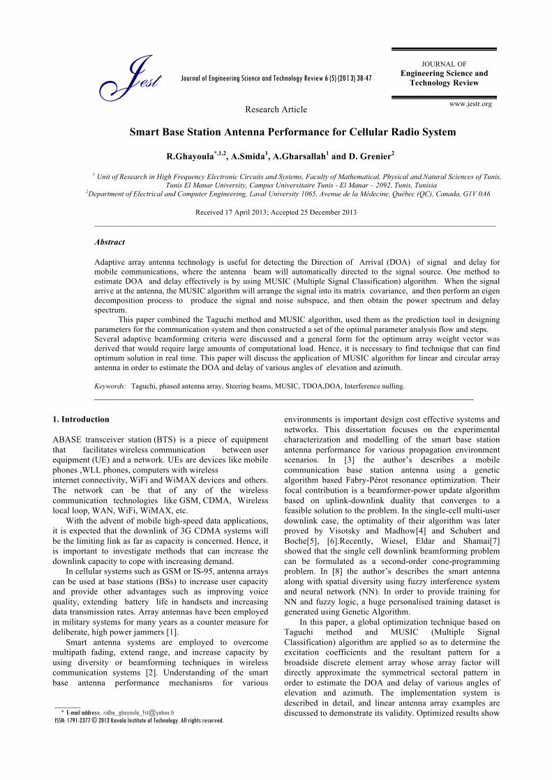
Fig.2. A wireless network with seven base-stations and three users per cell.


40

Fig. 3.A wireless network with seven base-stations and three users per cell. 3. Signal Model and Estimation Algorithm 3.1 Multiple Signal Classification Consider that the array antenna used for DOA estimation is a K-element linear array shown in Fig.1, and also that it receives L (L < K) narrow-band waves whose respective DOAs are 1θ , 2θ ,..., Lθ and complex amplitudes are ( )ts1 ,( )ts2 ,..., ( )tsL . When the array response vector (mode vector) of the lth

incoming wave is given by ( )la θ ( )Ll ;...;2;1= , the array input vector x(t) can be expressed as

( ) nutastxd

kkkk +=∑

=

),(.1

(1)

( ) nsAtx += . (2)

( ) ( ) ( ) ( ) ( ) ( )tntAstntsatx l

L

ll +=+=∑

=1

θ (3)

When x(t) and n(t) are column vectors of size [MF, 1]

(M: number of antennas and F: number of frequency points), and a matrix A with dimensions [MF, d] whose columns are the vectors a(tk,uk),1≤ k ≤ d defined by:

⎥⎥⎥⎥⎥⎥⎥⎥⎥⎥⎥⎥⎥⎥⎥⎥⎥⎥⎥

⎦

⎤

⎢⎢⎢⎢⎢⎢⎢⎢⎢⎢⎢⎢⎢⎢⎢⎢⎢⎢⎢

⎣

⎡

=

−−

−−

−−

−−

−−

−−

−−

−−

)...(..2

)..(..2

)..(..2

)...(..2

)...(..2

)...(..2

)...(..2

)...(..2

1

2

22

21

1

12

11

),(

kMkF

kMk

kkF

kk

kk

kkF

kk

kk

ugtfj

ugtfj

ugtfj

ugtfj

ugtfj

ugtfj

ugtfj

ugtfj

kk

e

e

e

eee

ee

uta

π

π

π

π

π

π

π

π

!

!!

!

!

∀ 1 ≤ k ≤ d

(4)

( ) ( ) ( )[ ]FF utautautaA ,,...,,,, 2211= (5)

( ) ( ) ( )[ ]Tl tststsS ,...,, 21=

(6) With

cxf

g mm

.0≈ , ∀ 1 ≤ m ≤ M

(7)

kku φsin= , ∀ 1 ≤ k ≤ d

(8) where A and s(t) are called the array response matrix

(mode matrix) and the signal vector, respectively, and n(t) is the internal additive noise vector[10]-[11].

The elements ( )tX and A are generally complex. A is a matrix dimension [ ]dFM ,. whose columns ( )kk uta , can be put in the form of Kronecker products:

)()(),( ktkukk tauauta ⊗= (9)

where

⎥⎥⎥⎥⎥⎥

⎦

⎤

⎢⎢⎢⎢⎢⎢

⎣

⎡

=

kM

km

k

ugj

ugj

ugj

ku

e

e

e

ua

....2

....2

....2 1

)(

π

π

π

!

! and

⎥⎥⎥⎥⎥⎥

⎦

⎤

⎢⎢⎢⎢⎢⎢

⎣

⎡

=

−

−

−

kF

kf

k

tfj

tfj

tfj

kt

e

e

e

ta

....2

....2

....2 1

)(

π

π

π

!

!, ∀ 1 ≤ k ≤ d

The kth column is a known function of the direction of

arrival and relative time delay of the kth path. The same element of the vector ( )ku ua , 1 ≤ m ≤ M,

depends on the relative position of the same sensor, the fth element of the vector ( )kt ta , 1≤ f ≤ F , depends on the fth frequency.

3.2. MUSIC Algorithm The most common techniques for DOA estimation can be distinguished between spectral based and parametric algorithms. Spectral based algorithms use a function, called pseudo spectrum, in which the maxima give an indication of the DOAs.

A large number of spectral based solutions have been proposed in literature, such as the Bartlett method, the Capon estimate, the linear prediction method, the maximum entropy method and many others [37].

A simple and widely adopted technique is the MUltiple SIgnal Classification (MUSIC) algorithm, which exploits the eigen structure properties of the array correlation matrix [38].

MUSIC (standing for multiple signal classification) is generally used in signal processing problems as a method for estimating the individual frequencies of multiple-harmonic signals. This is also the most frequently studied in the


41

literature, evidently with MUSIC see [12]-[13]-[14] and [15].

The MUSIC algorithm is the high-resolution method based on the eigenvectors of the covariance matrix of the array input vector. The covariance matrix is given by

( ) ( )[ ] IASAtxtxER HHxx

2σ+==

(10)

where ( ) ( )[ ]HtstsES = and 2σ is the power of internal noise. Then, the MUSIC spectrum is expressed as

2.

1

2

.

1

2

.),(

),(

.),(

),(.),(),(

∑

∑

+=

+=

=

=

FM

dkk

H

FM

dkk

H

H

MUSIC

wuta

uta

wuta

utautautP

(11)

( ) ( ) ( )( ) ( )θθ

θθθ

aEEaaaPHNN

H

H

MU =

(12)

[ ]KLN eeE ,...,1+= where NE is composed of the eigenvectors:{ }KL ee ,...,1+ spanning the noise subspace of the covariance matrix xxR .

3.3. Results and Discussion In this section, computer simulation results are provided to assess the performance with MUSIC Algorithm with different angles (AOA) and Time of arrivals (TDOA).

The MUSIC algorithm is implemented in MATLAB and tested by giving different angles as input to the system.

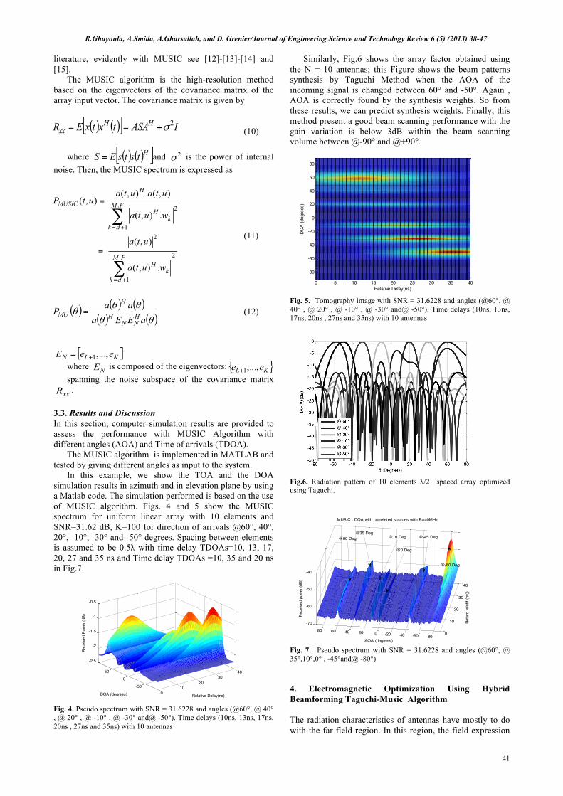
In this example, we show the TOA and the DOA simulation results in azimuth and in elevation plane by using a Matlab code. The simulation performed is based on the use of MUSIC algorithm. Figs. 4 and 5 show the MUSIC spectrum for uniform linear array with 10 elements and SNR=31.62 dB, K=100 for direction of arrivals @60°, 40°, 20°, -10°, -30° and -50° degrees. Spacing between elements is assumed to be 0.5λ with time delay TDOAs=10, 13, 17, 20, 27 and 35 ns and Time delay TDOAs =10, 35 and 20 ns in Fig.7.

Fig. 4. Pseudo spectrum with SNR = 31.6228 and angles (@60°, @ 40° , @ 20° , @ -10° , @ -30° and@ -50°). Time delays (10ns, 13ns, 17ns, 20ns , 27ns and 35ns) with 10 antennas

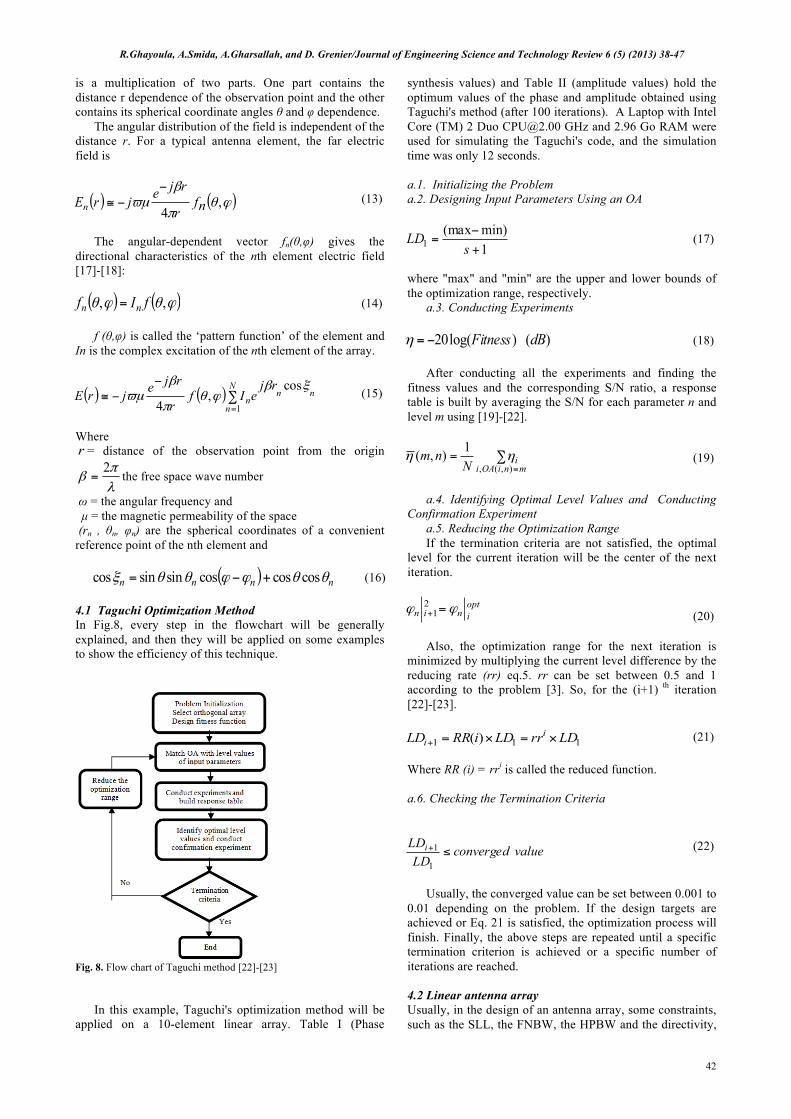
Similarly, Fig.6 shows the array factor obtained using the N = 10 antennas; this Figure shows the beam patterns synthesis by Taguchi Method when the AOA of the incoming signal is changed between 60° and -50°. Again , AOA is correctly found by the synthesis weights. So from these results, we can predict synthesis weights. Finally, this method present a good beam scanning performance with the gain variation is below 3dB within the beam scanning volume between @-90° and @+90°.

Fig. 5. Tomography image with SNR = 31.6228 and angles (@60°, @ 40° , @ 20° , @ -10° , @ -30° and@ -50°). Time delays (10ns, 13ns, 17ns, 20ns , 27ns and 35ns) with 10 antennas

Fig.6. Radiation pattern of 10 elements λ/2 spaced array optimized using Taguchi.

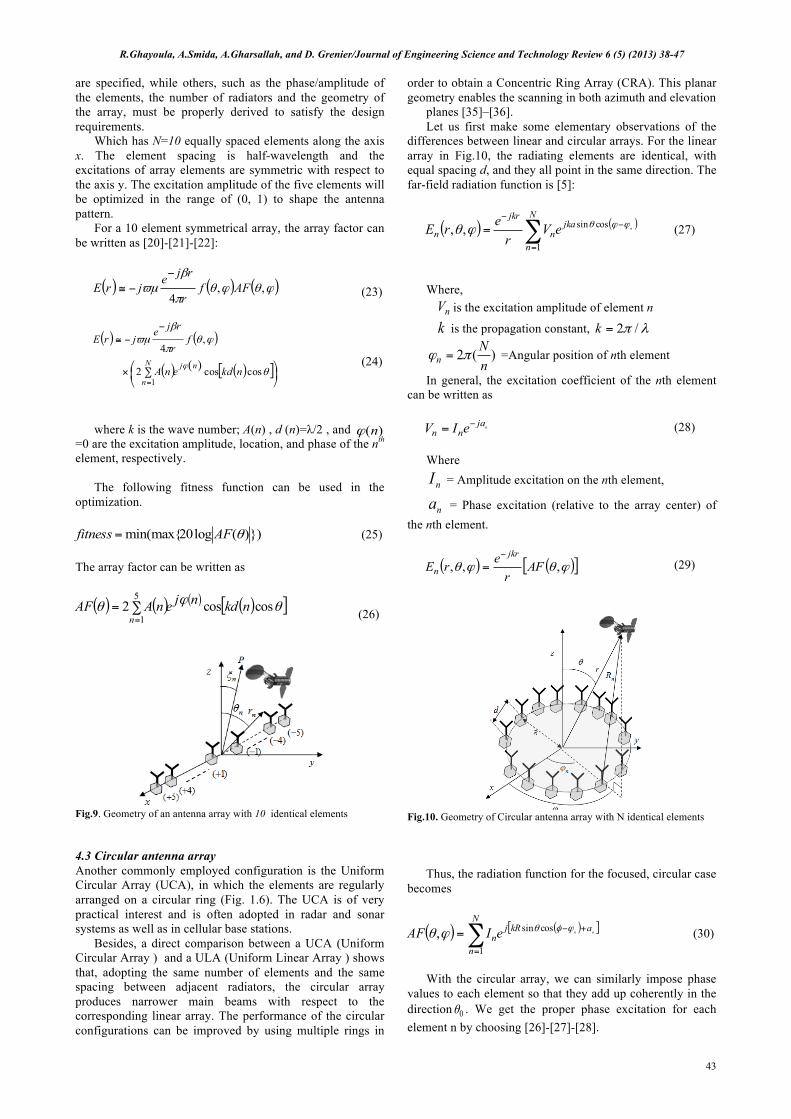
Fig. 7. Pseudo spectrum with SNR = 31.6228 and angles (@60°, @ 35°,10°,0° , -45°and@ -80°) 4. Electromagnetic Optimization Using Hybrid Beamforming Taguchi-Music Algorithm The radiation characteristics of antennas have mostly to do with the far field region. In this region, the field expression

010

2030

40

-50

0

50

-2.5

-2

-1.5

-1

-0.5

Relative Delay(ns)DOA (degrees)

Rece

ived

Pow

er (d

B)

0 5 10 15 20 25 30 35 40

-80

-60

-40

-20

0

20

40

60

80

Relative Delay(ns)

DOA

(deg

rees

)

0

10

20

30

40

-80-60-40-20020406080-70

-60

-50

-40

Reta

rd re

latif

(ns)

)

AOA (degrees)

MUSIC : DOA with correleted sources with B=40MHz

Rece

ived

pow

er (d

B)

@0 Deg

@35 Deg@10 Deg@60 Deg @-45 Deg

@-80 Deg


42

is a multiplication of two parts. One part contains the distance r dependence of the observation point and the other contains its spherical coordinate angles θ and φ dependence.

The angular distribution of the field is independent of the distance r. For a typical antenna element, the far electric field is

( ) ( )ϕθπ

βϖµ ,

4 nfr

rjejrEn−

−≅

(13)

The angular-dependent vector fn(θ,φ) gives the

directional characteristics of the nth element electric field [17]-[18]:

( ) ( )ϕθϕθ ,, fIf nn =

(14)

f (θ,φ) is called the ‘pattern function’ of the element and

In is the complex excitation of the nth element of the array.

( ) ( )∑−

−≅=

N

n

nnn

rjeIf

r

rjejrE1

cos,

4ξβ

ϕθπ

βϖµ

(15)

Where r = distance of the observation point from the origin

λπ

β2

= the free space wave number

ω = the angular frequency and µ = the magnetic permeability of the space (rn , θn, φn) are the spherical coordinates of a convenient reference point of the nth element and

( ) nnnn θθϕϕθθξ coscoscossinsincos +−=

(16)

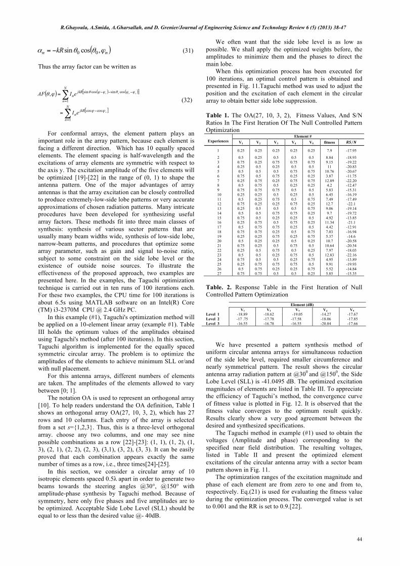
4.1 Taguchi Optimization Method In Fig.8, every step in the flowchart will be generally explained, and then they will be applied on some examples to show the efficiency of this technique.

Fig. 8. Flow chart of Taguchi method [22]-[23]

In this example, Taguchi's optimization method will be

applied on a 10-element linear array. Table I (Phase

synthesis values) and Table II (amplitude values) hold the optimum values of the phase and amplitude obtained using Taguchi's method (after 100 iterations). A Laptop with Intel Core (TM) 2 Duo [email protected] GHz and 2.96 Go RAM were used for simulating the Taguchi's code, and the simulation time was only 12 seconds.

a.1. Initializing the Problem a.2. Designing Input Parameters Using an OA

1min)(max

1 +−

=s

LD (17)

where "max" and "min" are the upper and lower bounds of the optimization range, respectively.

a.3. Conducting Experiments

)()log(20 dBFitness−=η (18)

After conducting all the experiments and finding the

fitness values and the corresponding S/N ratio, a response table is built by averaging the S/N for each parameter n and level m using [19]-[22].

∑==mniOAiiN

nm),(,

1),( ηη (19)

a.4. Identifying Optimal Level Values and Conducting

Confirmation Experiment a.5. Reducing the Optimization Range If the termination criteria are not satisfied, the optimal

level for the current iteration will be the center of the next iteration.

optinin ϕϕ =+

21

(20)

Also, the optimization range for the next iteration is

minimized by multiplying the current level difference by the reducing rate (rr) eq.5. rr can be set between 0.5 and 1 according to the problem [3]. So, for the (i+1) th iteration [22]-[23].

111 )( LDrrLDiRRLD ii ×=×=+

(21)

Where RR (i) = rri is called the reduced function.

a.6. Checking the Termination Criteria

valueconvergedLDLDi ≤+

1

1 (22)

Usually, the converged value can be set between 0.001 to

0.01 depending on the problem. If the design targets are achieved or Eq. 21 is satisfied, the optimization process will finish. Finally, the above steps are repeated until a specific termination criterion is achieved or a specific number of iterations are reached.

4.2 Linear antenna array Usually, in the design of an antenna array, some constraints, such as the SLL, the FNBW, the HPBW and the directivity,


43

are specified, while others, such as the phase/amplitude of the elements, the number of radiators and the geometry of the array, must be properly derived to satisfy the design requirements.

Which has N=10 equally spaced elements along the axis x. The element spacing is half-wavelength and the excitations of array elements are symmetric with respect to the axis y. The excitation amplitude of the five elements will be optimized in the range of (0, 1) to shape the antenna pattern.

For a 10 element symmetrical array, the array factor can be written as [20]-[21]-[22]:

( ) ( ) ( )ϕθϕθπ

βϖµ ,,

4AFf

r

rjejrE

−−≅

(23)

( ) ( )

( ) ( ) ( )[ ]⎟⎠⎞

⎜⎝⎛

∑×

−−≅

=θ

ϕθπ

βϖµ

ϕ coscos2

,4

1nkdenA

fr

rjejrE

njN

n

(24)

where k is the wave number; A(n) , d (n)=λ/2 , and )(nϕ

=0 are the excitation amplitude, location, and phase of the nth element, respectively.

The following fitness function can be used in the

optimization.

}))(log20min(max{ θAFfitness = (25)

The array factor can be written as

( ) ( ) ( ) ( )[ ]θϕθ coscos25

1nkdnjenAAF

n∑==

(26)

Fig.9. Geometry of an antenna array with 10 identical elements

4.3 Circular antenna array Another commonly employed configuration is the Uniform Circular Array (UCA), in which the elements are regularly arranged on a circular ring (Fig. 1.6). The UCA is of very practical interest and is often adopted in radar and sonar systems as well as in cellular base stations.

Besides, a direct comparison between a UCA (Uniform Circular Array ) and a ULA (Uniform Linear Array ) shows that, adopting the same number of elements and the same spacing between adjacent radiators, the circular array produces narrower main beams with respect to the corresponding linear array. The performance of the circular configurations can be improved by using multiple rings in

order to obtain a Concentric Ring Array (CRA). This planar geometry enables the scanning in both azimuth and elevation

planes [35]–[36]. Let us first make some elementary observations of the

differences between linear and circular arrays. For the linear array in Fig.10, the radiating elements are identical, with equal spacing d, and they all point in the same direction. The far-field radiation function is [5]:

( ) ( )njkaN

nn

jkr

n eVrerE ϕϕθϕθ −

=

−

∑= cossin

1

,,

(27)

Where, nV is the excitation amplitude of element n

k is the propagation constant, λπ /2=k

)(2nN

n πϕ = =Angular position of nth element

In general, the excitation coefficient of the nth element can be written as

nja

nn eIV −=

(28) Where

nI = Amplitude excitation on the nth element,

na = Phase excitation (relative to the array center) of the nth element.

( ) ( )[ ]ϕθϕθ ,,, AFrerEjkr

n

−

=

(29)

Fig.10. Geometry of Circular antenna array with N identical elements

Thus, the radiation function for the focused, circular case

becomes

( ) ( )[ ]nn akRjN

nneIAF +−

=∑= ϕφθϕθ cossin

1

,

(30)

With the circular array, we can similarly impose phase

values to each element so that they add up coherently in the direction 0θ . We get the proper phase excitation for each element n by choosing [26]-[27]-[28].


44

( )nn kR ϕθθα ,cossin 00−=

(31)

Thus the array factor can be written as

( ) ( ) ( )[ ]

[ ]∑

∑

=

−

=

−−−

=

=

N

n

jkRn

N

n

jkRn

eI

eIAF nn

1

coscos

1

cossincossin

0

00,

ψψ

ϕϕθϕϕθϕθ (32)

For conformal arrays, the element pattern plays an

important role in the array pattern, because each element is facing a different direction. Which has 10 equally spaced elements. The element spacing is half-wavelength and the excitations of array elements are symmetric with respect to the axis y. The excitation amplitude of the five elements will be optimized [19]-[22] in the range of (0, 1) to shape the antenna pattern. One of the major advantages of array antennas is that the array excitation can be closely controlled to produce extremely-low-side lobe patterns or very accurate approximations of chosen radiation patterns. Many intricate procedures have been developed for synthesizing useful array factors. These methods fit into three main classes of synthesis: synthesis of various sector patterns that are usually many beam widths wide, synthesis of low-side lobe, narrow-beam patterns, and procedures that optimize some array parameter, such as gain and signal to-noise ratio, subject to some constraint on the side lobe level or the existence of outside noise sources. To illustrate the effectiveness of the proposed approach, two examples are presented here. In the examples, the Taguchi optimization technique is carried out in ten runs of 100 iterations each. For these two examples, the CPU time for 100 iterations is about 6.5s using MATLAB software on an Intel(R) Core (TM) i3-2370M CPU @ 2.4 GHz PC.

In this example (#1), Taguchi's optimization method will be applied on a 10-element linear array (example #1). Table III holds the optimum values of the amplitudes obtained using Taguchi's method (after 100 iterations). In this section, Taguchi algorithm is implemented for the equally spaced symmetric circular array. The problem is to optimize the amplitudes of the elements to achieve minimum SLL or/and with null placement.

For this antenna arrays, different numbers of elements are taken. The amplitudes of the elements allowed to vary between [0; 1].

The notation OA is used to represent an orthogonal array [10]. To help readers understand the OA definition, Table I shows an orthogonal array OA(27, 10, 3, 2), which has 27 rows and 10 columns. Each entry of the array is selected from a set s={1,2,3}. Thus, this is a three-level orthogonal array. choose any two columns, and one may see nine possible combinations as a row [22]-[23]: (1, 1), (1, 2), (1, 3), (2, 1), (2, 2), (2, 3), (3,1), (3, 2), (3, 3). It can be easily proved that each combination appears exactly the same number of times as a row, i.e., three times[24]-[25].

In this section, we consider a circular array of 10 isotropic elements spaced 0.5λ apart in order to generate two beams towards the steering angles @30°, @150° with amplitude-phase synthesis by Taguchi method. Because of symmetry, here only five phases and five amplitudes are to be optimized. Acceptable Side Lobe Level (SLL) should be equal to or less than the desired value @- 40dB.

We often want that the side lobe level is as low as possible. We shall apply the optimized weights before, the amplitudes to minimize them and the phases to direct the main lobe.

When this optimization process has been executed for 100 iterations, an optimal control pattern is obtained and presented in Fig. 11.Taguchi method was used to adjust the position and the excitation of each element in the circular array to obtain better side lobe suppression. Table 1. The OA(27, 10, 3, 2), Fitness Values, And S/N Ratios In The First Iteration Of The Null Controlled Pattern Optimization

Experiences

Element # V1 V2 V3 V4 V5 fitness 𝑹𝑺 𝑵

1 0.25 0.25 0.25 0.25 0.25 7.9 -17.95

2 0.5 0.25 0.5 0.5 0.5 8.84 -18.93 3 0.75 0.25 0.75 0.75 0.75 9.15 -19.22 4 0.25 0.5 0.25 0.5 0.5 11 -20.83 5 0.5 0.5 0.5 0.75 0.75 10.76 -20.67 6 0.75 0.5 0.75 0.25 0.25 3.87 -11.75 7 0.25 0.75 0.25 0.75 0.75 12.89 -22.20 8 0.5 0.75 0.5 0.25 0.25 4.2 -12.47 9 0.75 0.75 0.75 0.5 0.5 5.83 -15.31 10 0.25 0.25 0.5 0.25 0.5 6.45 -16.19 11 0.5 0.25 0.75 0.5 0.75 7.49 -17.49 12 0.75 0.25 0.25 0.75 0.25 12.7 -22.1 13 0.25 0.5 0.5 0.5 0.75 9.06 -19.14 14 0.5 0.5 0.75 0.75 0.25 9.7 -19.72 15 0.75 0.5 0.25 0.25 0.5 4.92 -13.85 16 0.25 0.75 0.5 0.75 0.25 11.34 -21.1 17 0.5 0.75 0.75 0.25 0.5 4.42 -12.91 18 0.75 0.75 0.25 0.5 0.75 7.03 -16.94 19 0.25 0.25 0.75 0.25 0.75 5.37 -14.6 20 0.5 0.25 0.25 0.5 0.25 10.7 -20.58 21 0.75 0.25 0.5 0.75 0.5 10.64 -20.54 22 0.25 0.5 0.75 0.5 0.25 7.97 -18.03 23 0.5 0.5 0.25 0.75 0.5 12.83 -22.16 24 0.75 0.5 0.5 0.25 0.75 4.95 -13.89 25 0.25 0.75 0.75 0.75 0.5 9.91 -19.93 26 0.5 0.75 0.25 0.25 0.75 5.52 -14.84 27 0.75 0.75 0.5 0.5 0.25 5.85 -15.35

Table. 2. Response Table in the First Iteration of Null Controlled Pattern Optimization

We have presented a pattern synthesis method of uniform circular antenna arrays for simultaneous reduction of the side lobe level, required smaller circumference and nearly symmetrical pattern. The result shows the circular antenna array radiation pattern at @300 and @1500, the Side Lobe Level (SLL) is -41.0495 dB. The optimized excitation magnitudes of elements are listed in Table III. To appreciate the efficiency of Taguchi’s method, the convergence curve of fitness value is plotted in Fig. 12. It is observed that the fitness value converges to the optimum result quickly. Results clearly show a very good agreement between the desired and synthesized specifications.

The Taguchi method in example (#1) used to obtain the voltages (Amplitude and phase) corresponding to the specified near field distribution. The resulting voltages, listed in Table II and present the optimized element excitations of the circular antenna array with a sector beam pattern shown in Fig. 11.

The optimization ranges of the excitation magnitude and phase of each element are from zero to one and from to, respectively. Eq.(21) is used for evaluating the fitness value during the optimization process. The converged value is set to 0.001 and the RR is set to 0.9.[22].

Element (dB) V1 V2 V3 V4 V5

Level 1 -18.89 -18.62 -19.05 -14.27 -17.67 Level 2 -17 .75 -17.78 -17.58 -18.06 -17.85 Level 3 -16.55 -16.78 -16.55 -20.84 -17.66

Match OA with level values of input parameters


45

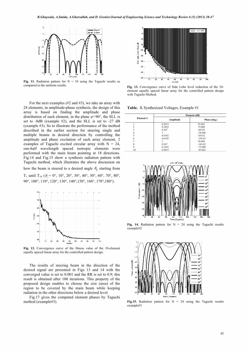
Fig. 11. Radiation pattern for N = 10 using the Taguchi results as compared to the uniform results

For the next examples (#2 and #3), we take an array with

24 elements, in amplitude-phase synthesis, the design of this array is based on finding the amplitude and phase distribution of each element, in the plane φ=90°, the SLL is set to -8dB (example #2), and the SLL is set to -27 dB (example #3). So to illustrate the performance of the method described in the earlier section for steering single and multiple beams in desired direction by controlling the amplitude and phase excitation of each array element, 2 examples of Taguchi excited circular array with N = 24, one-half wavelength spaced isotropic elements were performed with the main beam pointing at 18 directions. Fig.14 and Fig.15 show a synthesis radiation pattern with Taguchi method, which illustrates the above discussion on how the beam is steered to a desired angle 0θ starting from

T1 until T18 ( !θ = 0°, 10°, 20°, 30°, 40°, 50°, 60°, 70°, 80°, 90°, 100°, 110°, 120°, 130°, 140°,150°, 160°, 170°,180°).

Fig. 12. Convergence curve of the fitness value of the 10-element equally spaced linear array for the controlled pattern design.

The results of steering beam in the direction of the desired signal are presented in Figs 13 and 14 with the converged value is set to 0.001 and the RR is set to 0.9; this result is obtained after 100 iterations. This property of the proposed design enables to choose the size (area) of the region to be covered by the main beam while keeping radiation in the other directions below a desired level.

Fig.17 gives the computed element phases by Taguchi method (example#3).

Fig. 13. Convergence curve of Side Lobe level reduction of the 10-element equally spaced linear array for the controlled pattern design with Taguchi Method.

Table. 3. Synthesized Voltages, Example #1

Fig. 14. Radiation pattern for N = 24 using the Taguchi results example#2

Fig.15. Radiation pattern for N = 24 using the Taguchi results example#3

Element #

Element (dB)

Amplitude Phase (deg.)

1 0.2015 93.863 2 0.1452 75.008 3 0.367 165.03 4 1 -30.496 5 0.6182 145.62 6 0.6182 -145.62 7 1 30.496 8 0.367 -165.03 9 0.1452 -75.008 10 0.2015 -93.863


46

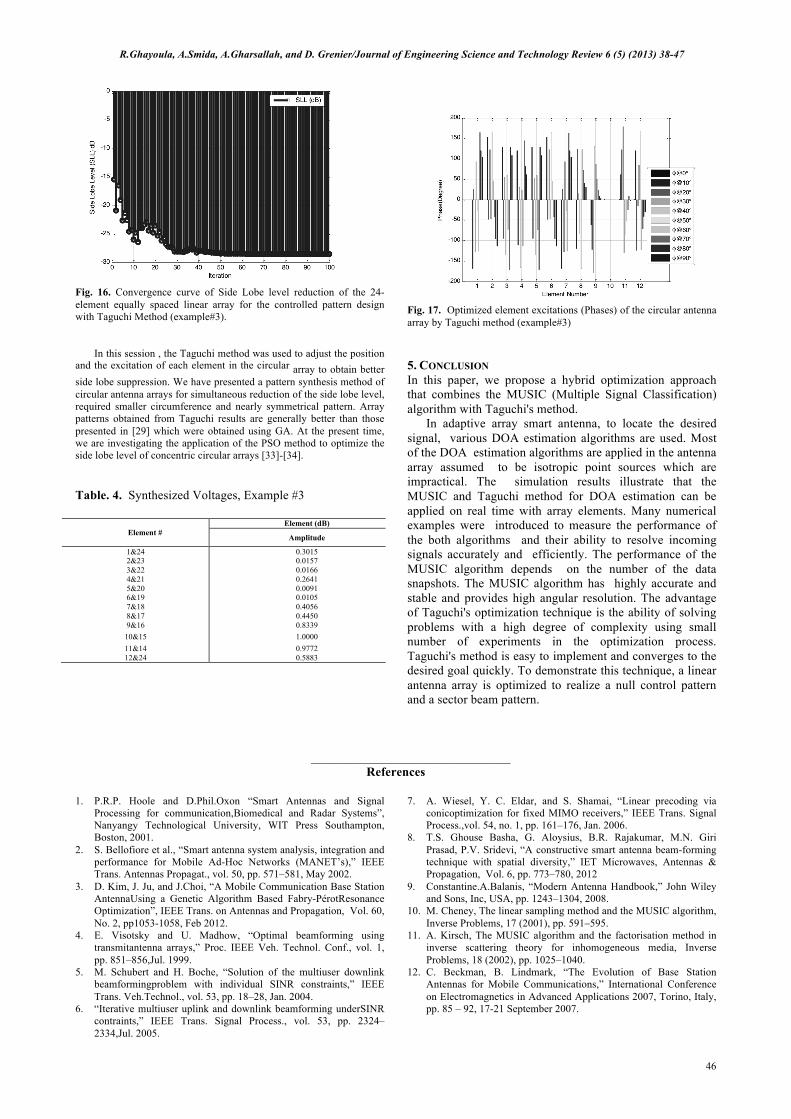
Fig. 16. Convergence curve of Side Lobe level reduction of the 24-element equally spaced linear array for the controlled pattern design with Taguchi Method (example#3).

In this session , the Taguchi method was used to adjust the position

and the excitation of each element in the circular array to obtain better side lobe suppression. We have presented a pattern synthesis method of circular antenna arrays for simultaneous reduction of the side lobe level, required smaller circumference and nearly symmetrical pattern. Array patterns obtained from Taguchi results are generally better than those presented in [29] which were obtained using GA. At the present time, we are investigating the application of the PSO method to optimize the side lobe level of concentric circular arrays [33]-[34]. Table. 4. Synthesized Voltages, Example #3

Fig. 17. Optimized element excitations (Phases) of the circular antenna array by Taguchi method (example#3)

5. CONCLUSION In this paper, we propose a hybrid optimization approach that combines the MUSIC (Multiple Signal Classification) algorithm with Taguchi's method.

In adaptive array smart antenna, to locate the desired signal, various DOA estimation algorithms are used. Most of the DOA estimation algorithms are applied in the antenna array assumed to be isotropic point sources which are impractical. The simulation results illustrate that the MUSIC and Taguchi method for DOA estimation can be applied on real time with array elements. Many numerical examples were introduced to measure the performance of the both algorithms and their ability to resolve incoming signals accurately and efficiently. The performance of the MUSIC algorithm depends on the number of the data snapshots. The MUSIC algorithm has highly accurate and stable and provides high angular resolution. The advantage of Taguchi's optimization technique is the ability of solving problems with a high degree of complexity using small number of experiments in the optimization process. Taguchi's method is easy to implement and converges to the desired goal quickly. To demonstrate this technique, a linear antenna array is optimized to realize a null control pattern and a sector beam pattern.

______________________________

References 1. P.R.P. Hoole and D.Phil.Oxon “Smart Antennas and Signal

Processing for communication,Biomedical and Radar Systems”, Nanyangy Technological University, WIT Press Southampton, Boston, 2001.

2. S. Bellofiore et al., “Smart antenna system analysis, integration and performance for Mobile Ad-Hoc Networks (MANET’s),” IEEE Trans. Antennas Propagat., vol. 50, pp. 571–581, May 2002.

3. D. Kim, J. Ju, and J.Choi, “A Mobile Communication Base Station AntennaUsing a Genetic Algorithm Based Fabry-PérotResonance Optimization”, IEEE Trans. on Antennas and Propagation, Vol. 60, No. 2, pp1053-1058, Feb 2012.

4. E. Visotsky and U. Madhow, “Optimal beamforming using transmitantenna arrays,” Proc. IEEE Veh. Technol. Conf., vol. 1, pp. 851–856,Jul. 1999.

5. M. Schubert and H. Boche, “Solution of the multiuser downlink beamformingproblem with individual SINR constraints,” IEEE Trans. Veh.Technol., vol. 53, pp. 18–28, Jan. 2004.

6. “Iterative multiuser uplink and downlink beamforming underSINR contraints,” IEEE Trans. Signal Process., vol. 53, pp. 2324–2334,Jul. 2005.

7. A. Wiesel, Y. C. Eldar, and S. Shamai, “Linear precoding via conicoptimization for fixed MIMO receivers,” IEEE Trans. Signal Process.,vol. 54, no. 1, pp. 161–176, Jan. 2006.

8. T.S. Ghouse Basha, G. Aloysius, B.R. Rajakumar, M.N. Giri Prasad, P.V. Sridevi, “A constructive smart antenna beam-forming technique with spatial diversity,” IET Microwaves, Antennas & Propagation, Vol. 6, pp. 773–780, 2012

9. Constantine.A.Balanis, “Modern Antenna Handbook,” John Wiley and Sons, Inc, USA, pp. 1243–1304, 2008.

10. M. Cheney, The linear sampling method and the MUSIC algorithm, Inverse Problems, 17 (2001), pp. 591–595.

11. A. Kirsch, The MUSIC algorithm and the factorisation method in inverse scattering theory for inhomogeneous media, Inverse Problems, 18 (2002), pp. 1025–1040.

12. C. Beckman, B. Lindmark, “The Evolution of Base Station Antennas for Mobile Communications,” International Conference on Electromagnetics in Advanced Applications 2007, Torino, Italy, pp. 85 – 92, 17-21 September 2007.

Element #

Element (dB)

Amplitude

1&24 0.3015

2&23 0.0157

3&22 0.0166

4&21 0.2641

5&20 0.0091

6&19 0.0105

7&18 0.4056

8&17 0.4450

9&16 0.8339

10&15 1.0000

11&14 0.9772

12&24 0.5883


47

13. J. Modelski and Y. Yashchyshyn, “Voltage-controlled ferroelectric smart antenna,” IEEE Antennas Propag.Sym. Vol.2,pp.506-509, Jully 2000.

14. C. W. Therrien, Discrete Random Signals and Statistical Signal Processing, Prentice–Hall, Englewood Cliffs, NJ, 1992.

15. S. K. Lehman and A. J. Devaney, Transmission mode time-reversal super-resolution imaging, J. Acoust. Soc. Amer., 113 (2003), pp. 2742–2753.

16. T. D. Mast, A. I. Nachman, and R. C. Waag, Focusing and imaging using eigenfunctions of the scattering operator, J. Acoust. Soc. Amer., 102 (1997), pp. 715–725.

17. G. A. Rafael, L. H. Fernando, L. F. Herrán, “Neural Modeling of Mutual Coupling for Antenna Array Synthesis”, IEEE Trans. Antennas Propagat., Vol. 55, pp. 832-840, 2007.

18. R. Ghayoula, N. Fadlallah, A. Gharsallah, M. Rammal, IET Microw. Antennas Propag., “Phase-Only Adaptive Nulling with Neural Networks for Antenna Array Synthesis”, Vol. 3, pp.154-163, 2009.

19. N. Nemri, A. Smida, R. Ghayoula, H. Trabelsi and A. Gharsallah,” Synthesis and implementation of Phased Circular Antenna Arrays Using Taguchi Method”, Information Processing and Wireless Systems, IP-WiS 2012, March 16-18, 2012 Sousse, Tunisia

20. A. Smida, R. Ghayoula, A. Troudi, H. Trabelsi, A. Gharsallah , “Beam Synthesis of Phased Circular Antenna Arrays Using Taguchi Method”, 9th International Conference on Communications COMM 2012, National Military Center Bucharest, 21 -23 Jun 2012, Romania

21. A. Smida, R. Ghayoula and A. Gharsallah,” Synthesis of Phased Cylindrical Arc Antenna Arrays Using Taguchi Method”, Information Processing and Wireless Systems, IP-WiS 2012, March 16-18, 2012 Sousse, Tunisia

22. Weng, W., F. Yang, and A. Elsherbeni, “Linear antenna array synthesis using Taguchi's method: A novel optimization technique in electromagnetics,” IEEE Trans. on Antennas and Propagation, Vol. 55, 723-730, 2007

23. Weng, W. C. and C. Choi, “Optimal design of CPW slot antennasusing Taguchi's method," IEEE Trans. on Magnetics, Vol. 45,No. 3, 1542-1545, Mar. 2009.

24. J. N. Sahalos “Orthogonal Methods for Array Synthesis: Theory and the ORAMA Computer Tool”, John Wiley & Sons, 2006

25. J. N. Sahalos “Orthogonal Methods for Array Synthesis: Theory and the ORAMA Computer Tool”, John Wiley & Sons, 2006

26. Dessouky, M. I., H. A. Sharshar, and Y. A. Albagory, Efficient sidelobe reduction technique for small-sized concentric circular arrays," Progress In Electromagnetics Research, PIER 65, 187-200, 2006.

27. Chen, T. B., Y. L. Dong, Y. C. Jiao, and F. S. Zhang,”Synthesis of circular antenna array using crossed particle swarm optimization algorithm," Journal of Electromagnetic Waves and Applications,Vol. 20, No. 13, 1785{1795, 2006.

28. Joaquim A. R. Azevedo , “Synthesis of Planar Arrays With Elements in Concentric Rings”, IEEE Trans. on Antennas and Propagation, vol. 59, NO. 3, pp. 839-845, 2011.

29. K. K. Yan and Y.Lu,“Sidelobe Reduction in Array-Pattern Synthesis using Genetic Algorithm”, IEEE Trans. on Antennas and Propagation, vol. 45, NO. 7,1997

30. G. Taguchi, S. Chowdhury, and Y.Wu, Taguchi’s Quality Engineering Handbook. New York: Wiley, 2005.

31. Roy R., “Design of Experiments Using the Taguchi Approach: 16 Steps to Product and Process Improvement”, John Wiley and Sons. 2001.

32. A. Smida, L. Gargouri, R. Ghayoula, H. Trabelsi and A. Gharsallah, “Amplitude-only adaptive nulling based on taguchi’s method”, Multi-Conference on Systems, Signals & Devices SSD’11, Tunisia, March 22-25, 2011

33. M. Clerc and J. Kennedy, “The Particle Swarm–Explosion, Stability, and Convergence in the Multidimensional Complex Space,” IEEE Trans. on Evolutionary Computation, Vol. 6, No. 1, pp. 58–73. Feb. 2002

34. J. Robinson and Y. Rahmat-Samii, “Particle Swarm Optimization in Electromagnetics,” IEEE Trans. on Antennas and Propagation, Vol. 52, No. 2., pp. 397–407, Feb. 2004.

35. P. Ioannides and C.A. Balanis, “Uniform Circular Arrays for Smart Antennas,” IEEE Antennas and Propagation Magazine, vol. 47, no. 4, pp. 192–206, Aug. 2005.

36. “Uniform Circular and Rectangular Arrays for Adaptive Beamforming Applications,” IEEE Antennas andWireless Propagation Letters, vol. 4, pp. 351–354, 2005.

37. F. Gross, Smart Antennas for Wireless Communications with Matlab. New York, McGraw-Hill, 2005.

38. L.C. Godara, “Application of Antenna Arrays to Mobile Communications, Part II: Beam Forming and Direction-of-Arrival Considerations,” Proceedings of the IEEE, vol. 85, no. 8, pp. 1193–1245, Aug. 1997.

Documents

Smart Base Station Antenna Performance for Cellular Radio ... · PDF fileSmart Base Station Antenna Performance for Cellular Radio System ... based on uplink-downlink duality that