Slope and Embankment Stability - Civil Engineeringbartlett/CVEEN5305/Slope Stability… · · 2015-12-12Slope and Embankment Stability Thursday, March 11, 2010 11:43 AM Slope Stability

Steven F. Bartlett, 2010

Lecture Notes○

Reading Assignment

Homework Assignment

Obtain an install the visual slope software on your computer.1.

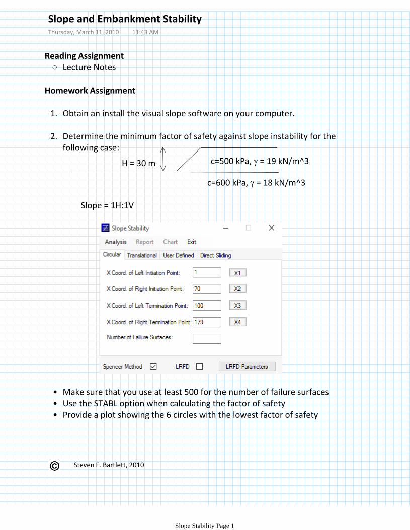
Determine the minimum factor of safety against slope instability for the following case:

2.

c=600 kPa, = 18 kN/m^3

Slope = 1H:1V

Make sure that you use at least 500 for the number of failure surfaces•Use the STABL option when calculating the factor of safety•Provide a plot showing the 6 circles with the lowest factor of safety•

c=500 kPa, = 19 kN/m^3H = 30 m

Slope and Embankment StabilityThursday, March 11, 2010 11:43 AM

Slope Stability Page 1


Lecture Notes○

Reading Assignment

For the case given in problem 2, determine the minimum factor of safety for the slope given in problem 2 when a 0.5 g horizontal seismic acceleration is applied.

3.

= 135 pcfi.

' = 35 degii.

Embankment propertiesa.

= 100 pcfi.

sat = 120 pcfii.

' = 14 degiii.c' = 100 psfiv.

Foundation soil propertiesb.

Water table is found 6.56 ft below the top of the foundation soilc.

Use Spencer's method to determine the maximum height that an 2H:1V sloped earthen embankment can be constructed on a weak foundation soil with a F.S. = 1.3 given the following:

4.

Homework Assignment (cont.)

Slope and Embankment StabilityThursday, March 11, 2010 11:43 AM



Slope, embankment and excavation stability analyses are used in a wide variety of geotechnical engineering problems, including, but not limited to, the following:

• Determination of stable cut and fill slopes

• Assessment of overall stability of retaining walls, including globaland compound stability (includes permanent systems and temporaryshoring systems)

• Assessment of overall stability of shallow and deep foundations forstructures located on slopes or over potentially unstable soils, includingthe determination of lateral forces applied to foundations and walls dueto potentially unstable slopes

• Stability assessment of landslides (mechanisms of failure, anddetermination of design properties through back-analysis), and designof mitigation techniques to improve stability

• Evaluation of instability due to liquefaction

(From WASDOT manual of instruction)

Slope and Embankment Stability (cont.)Thursday, March 11, 2010 11:43 AM



General Types of Mass Movement

Morphology of a Typical Soil Slump

Types of Mass Movement (i.e., Landsliding)Thursday, March 11, 2010 11:43 AM



Whether long-term or short-term stability is in view, and which will controlthe stability of the slope, will affect the selection of soil and rock shearstrength parameters used as input in the analysis.

For short-term stability analysis, undrained shear strength parameters should be obtained. Short-term conditions apply for rapid loadings and for cases where construction is completed rapidly (e.g. rapid raise of embankments, cutting of slopes, etc.)

For long-term stability analysis, drained shear strength parameters should be obtained. Long-term conditions imply that the pore pressure due to the loading have dissipated and the equilibrium pore pressures have been reached.

For assessing the stability of landslides, residual shear strength parameterswill be needed, since the soil has in such has typically deformed enough toreach a residual value. This implies that the slope or soil has previously failed along a failure plane and the there is potential for reactivation of the failure along this plane.

For highly overconsolidated clays, such as the Seattle clays (e.g., Lawton Formation), if the slope is relatively free to deform after the cut is made or is otherwise unloaded, residual shear strength parameters should be obtained and used for the stability analysis.

Required Soil ParametersThursday, March 11, 2010 11:43 AM



Factors of safety for slopes other than the slopes of dams should be selected consistent with the uncertainty involved in the parameters such as shear strength and pore water pressures that affect the calculated value of factor of safety and the consequences of failure. When the uncertainty and the consequences of failure are both small, it is acceptable to use small factors of safety, on the order of 1.3 or even smaller in some circumstances.

When the uncertainties or the consequences of failure increase, larger factors of safety are necessary. Large uncertainties coupled with large consequences of failure represent an unacceptable condition, no matter what the calculated value of the factor of safety.

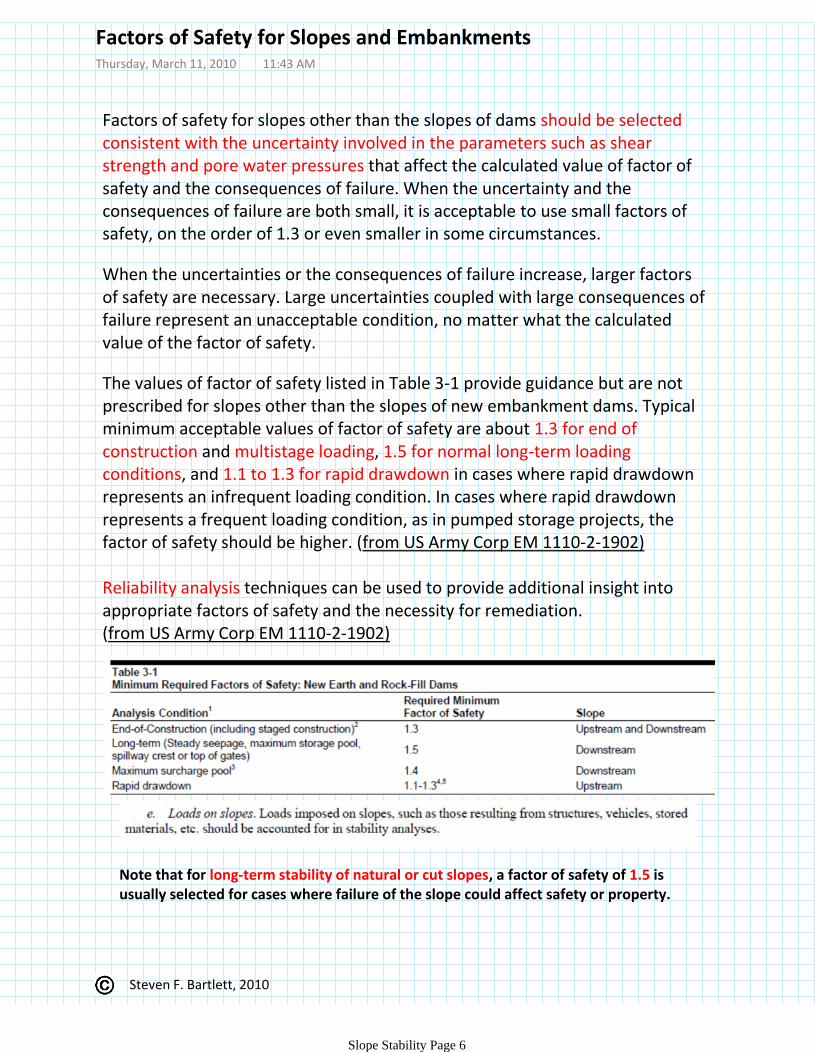
The values of factor of safety listed in Table 3-1 provide guidance but are not prescribed for slopes other than the slopes of new embankment dams. Typical minimum acceptable values of factor of safety are about 1.3 for end of construction and multistage loading, 1.5 for normal long-term loading conditions, and 1.1 to 1.3 for rapid drawdown in cases where rapid drawdown represents an infrequent loading condition. In cases where rapid drawdown represents a frequent loading condition, as in pumped storage projects, the factor of safety should be higher. (from US Army Corp EM 1110-2-1902)

Reliability analysis techniques can be used to provide additional insight into appropriate factors of safety and the necessity for remediation.(from US Army Corp EM 1110-2-1902)

Note that for long-term stability of natural or cut slopes, a factor of safety of 1.5 is usually selected for cases where failure of the slope could affect safety or property.

Factors of Safety for Slopes and EmbankmentsThursday, March 11, 2010 11:43 AM



Conventional approach.

The figure above shows a potential slide mass defined by a candidate slip surface. If the shear resistance of the soil along the slip surface exceeds that necessary to provide equilibrium, the mass is stable. If the shear resistance is insufficient, the mass is unstable.

Conventional slope stability analyses investigate the equilibrium of a mass of soil bounded below by an assumed potential slip surface and above by the surface of the slope. Forces and moments tending to cause instability of the mass are compared to those tending to resist instability. Most procedures assume a two-dimensional (2-D)cross section and plane strain conditions for analysis. Successive assumptions are made regarding the potential slip surface until the most critical surface (lowest factor ofsafety) is found. The stability or instability of the mass depends on its weight, the external forces acting on it (such as surcharges or accelerations caused by dynamic loads), the shear strengths and porewater pressures along the slip surface, and the strength of any internal reinforcement crossing potential slip surfaces.

LE Methods - BasicsThursday, March 11, 2010 11:43 AM



Factor of Safety

For effective stress analyses

For total stress analyses

Limit Equilibrium Method (LE) - The portion or part of the shear stress mobilized along the potential shear surface is related to the shear strength and the factor of safety using the equation below, which has been written for the case of effective stress analysis.

Note that in the above equation there is a shear resistance component attributed to the cohesion component, c', and a component attributed to the frictional part

(-u)tan '. In developing the LE method, it is assumed that both components develop or mobilize their respective shear resistance as the same rate.

LE Methods - Basics (cont.)Thursday, March 11, 2010 11:43 AM



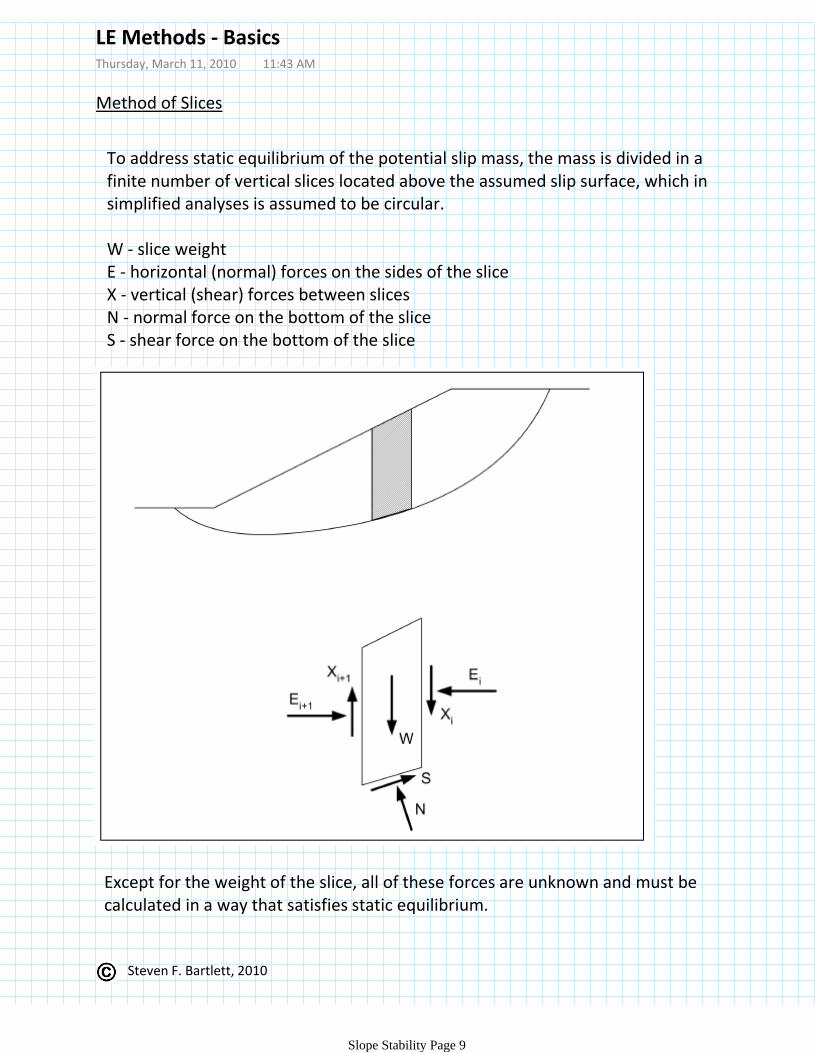
Method of Slices

To address static equilibrium of the potential slip mass, the mass is divided in a finite number of vertical slices located above the assumed slip surface, which in simplified analyses is assumed to be circular.

W - slice weightE - horizontal (normal) forces on the sides of the sliceX - vertical (shear) forces between slicesN - normal force on the bottom of the sliceS - shear force on the bottom of the slice

Except for the weight of the slice, all of these forces are unknown and must be calculated in a way that satisfies static equilibrium.




Note that for the current discussion, the shear force (S) on the bottom of the slice is not considered as entirely unknown in the equilibrium equations that are solved. Instead, this shear force can be expressed in terms of other known and unknown quantities, as follows:

S on the base of a slice is equal to the shear stress, τ, multiplied by the length of the base of the slice, Δl

S = τ Δl

Hence using the below equation for (previous), S, can be written to:

can be rewritten to:

Finally, noting that the normal force N is equal to the product of the normal stress (σ) and the length of the bottom of the slice (Δl), i.e., N = σ Δl, the above equation can be written as:

This fundamental equation for the method of slices relates the shear force, S, to the normal force on the bottom of the slice and the factor of safety. Thus, if the normal force and factor of safety can be calculated from the equations of staticequilibrium, the shear force can be calculated from this equation.




The fundamental equation was derived from the Mohr-Coulomb equation and the definition of the factor of safety, independently of the conditions of static equilibrium. The forces and other unknowns that must be calculated from the equilibrium equations are summarized in the below table. As discussed above, the shear force, S, is not included in this table, because it can be calculated from the unknowns listed and the Mohr-Coulomb equation independently of staticequilibrium equations.

In order to achieve a statically determinate solution, there must be a balance between the number of unknowns and the number of equilibrium equations. The number of equilibrium equations is shown in the lower part of Table C-1. The number of unknowns (5n – 2) exceeds the number of equilibrium equations (3n) if n is greater than one. Therefore, some assumptions must be made to achieve a statically determinate solution.

The various limit equilibrium methods use different assumptions to make the number of equations equal to the number of unknowns. They also differ with regard to which equilibrium equations are satisfied. For example, the Ordinary Method of Slices, the Simplified Bishop Method, and the U.S. Army Corps of Engineers’ Modified Swedish Methods do not satisfy all the conditions of static equilibrium. Methods such as the Morgenstern and Price’s and Spencer’s do satisfy all static equilibrium conditions. Methods that satisfy static equilibrium fully are referred to as “complete” equilibrium methods. Detailed comparison of limit equilibrium slope stability analysis methods have been reported by Whitman and Bailey (1967), Wright (1969), Duncan and Wright (1980) and Fredlund and Krahn (1977).




Most common LE method is the method of slices○

Ordinary Method of Slices

Modified or Simplified Bishop

Taylor

Spencer

Spencer-Wright

Janbu

Fellenius (Swedish)

Morgenstern

Morgenstern-Price

US Army Corp of Engineers

Bell

Sharma

General Limit Equilibrium Methods (GLE)

Methods/Researchers○

Limit Equilibrium

Analysis Methods - Limit EquilibriumThursday, March 11, 2010 11:43 AM



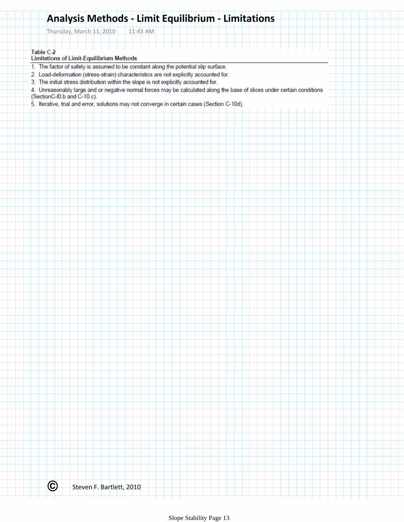
Analysis Methods - Limit Equilibrium - LimitationsThursday, March 11, 2010 11:43 AM



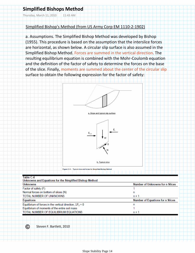
Simplified Bishop's Method (from US Army Corp EM 1110-2-1902)

a. Assumptions. The Simplified Bishop Method was developed by Bishop (1955). This procedure is based on the assumption that the interslice forces are horizontal, as shown below. A circular slip surface is also assumed in the Simplified Bishop Method. Forces are summed in the vertical direction. The resulting equilibrium equation is combined with the Mohr-Coulomb equation and the definition of the factor of safety to determine the forces on the base of the slice. Finally, moments are summed about the center of the circular slipsurface to obtain the following expression for the factor of safety:

Simplified Bishops MethodThursday, March 11, 2010 11:43 AM



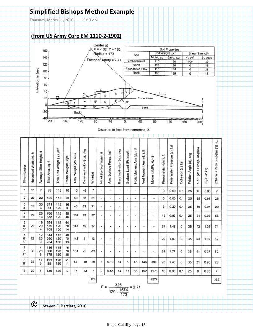
(from US Army Corp EM 1110-2-1902)

Simplified Bishops Method ExampleThursday, March 11, 2010 11:43 AM



Limitations. Horizontal equilibrium of forces is not satisfied by the Simplified Bishop Method. Because horizontal force equilibrium is not completely satisfied, the suitability of the Simplified Bishop Method for pseudo-static earthquake analyses where an additional horizontal force is applied is questionable. The method is also restricted to analyses with circular shear surfaces.

Recommendation for use. It has been shown by a number of investigators that the factors of safety calculated by the Simplified Bishop Methodcompare well with factors of safety calculated using rigorous methods, usually within 5 percent. Furthermore, the procedure is relatively simple compared to more rigorous solutions, computer solutions execute rapidly, and hand calculations are not very time-consuming. The method is widely used throughout the world, and thus, a strong record of experience with the method exists. The Simplified Bishop Method is an acceptable method of calculating factors of safety for circular slip surfaces. It is recommended that, where major structures are designed using the Simplified Bishop Method, the final design should be checked using Spencer’s Method.

Verification procedures. When the Simplified Bishop Method is used for computer calculations, results can be verified by hand calculations using a calculator or a spreadsheet program, or using slope stability charts. An approximate check of calculations can also be performed using the Ordinary Method of Slices, although the OMS will usually give a lower value for the factor of safety, especially if φ is greater than zero and pore pressures are high.

Simplified Bishops Method - Misc.Thursday, March 11, 2010 11:43 AM



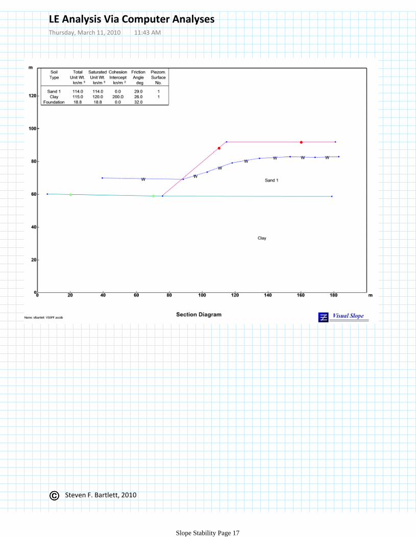
LE Analysis Via Computer AnalysesThursday, March 11, 2010 11:43 AM



LE Analysis Via Computer Analyses (cont.)Thursday, March 11, 2010 11:43 AM



LE Analysis Methods - References Thursday, March 11, 2010 11:43 AM



51st Rankine Lecture

Geotechnical Stability Analysis

Professor Scott W Sloan

University of Newcastle,NSW, Australia

ABSTRACT

Historically, geotechnical stability analysis has been performed by a variety of approximate methods that are based on the notion of limit equilibrium. Although they appeal to engineering intuition, these techniques have a number of major disadvantages, not the least of which is the need to presuppose an appropriate failure mechanism in advance. This feature can lead to inaccurate predictions of the true failure load, especially for cases involving layered materials, complex loading, or three-dimensional deformation.

This lecture will describe recent advances in stability analysis which avoid these shortcomings. Attention will be focused on new methods which combine the limit theorems of classical plasticity with finite elements to give rigorous upper and lower bounds on the failure load. These methods, known as finite element limit analysis, do not require assumptions to be made about the mode of failure, and use only simple strength parameters that are familiar to geotechnical engineers. The bounding properties of the solutions are invaluable in practice, and enable accurate solutions to be obtained through the use of an exact error estimate and automatic adaptive meshing procedures. The methods are extremely general and can deal with layered soil profiles, anisotropic strength characteristics, fissured soils, discontinuities, complicated boundary conditions, and complex loading in both two and three dimensions. Following a brief outline of the new techniques, stability solutions for a number of practical problems will be given including foundations, anchors, slopes, excavations, and tunnels.

Numerical MethodsThursday, March 11, 2010 11:43 AM



Numerical Modeling (FDM and FEM)

Any failure mode develops naturally; there is no need to specify a range of trial surfaces in advance.

•

No artificial parameters (e.g., functions for inter-slice angles) need to be given as input.

•

Multiple failure surfaces (or complex internal yielding) evolve naturally, if the conditions give rise to them.

•

Structural interaction (e.g., rock bolt, soil nail or geogrid) is modeled realistically as fully coupled deforming elements, not simply as equivalent forces.

•

Solution consists of mechanisms that are feasible kinematically.•

Numerical model such as FLAC offers these advantages over Limit Equilibrium methods:

Pasted from <http://www.itascacg.com/flacslope/overview.html>

There are a number of methods that could have been employed to determine the factor of safety using FLAC. The FLAC shear strength reduction (SSR) method of computing a factor of safety performs a series of computations to bracket the range of possible factors of safety. During SSR, the program lowers the strength (angle) of the soil and computes the maximum unbalanced force to determine if the slope is moving. If the force unbalance exceeds a certain value, the strength is increased and the original stresses returned to the initial value and the deformation analyses recomputed. This process continues until the force unbalance is representative of the initial movement of the slope and the angle for this condition is compared to the angle available for the soil to compute the factor of safety.

Numerical MethodsThursday, March 11, 2010 11:43 AM


http://www.itascacg.com/flacslope/overview.html


In FLAC, the yield criterion for problems involving plasticity is expressed in terms of effective stresses. The strength parameters used for input in a fully coupled mechanical-fluid flow problem are drained properties. Also, whenever CONFIG gw is selected: a) the drained bulk modulus of the material should be used if the fluid bulk modulus is specified; and b) the dry mass density of the material should be specified when the fluid density is given. The apparent volumetric and strength properties of the medium will then evolve with time, because they depend on the pore pressure generated during loading and dissipated during drainage. The dependence of apparent properties on the rate of application of load and drainage is automatically reflected in a coupled calculation, even when constant input properties are specified.

Effective stress analysis (drained parameters) (if pore pressure due to loading can be estimated)

○

Total stress analysis (undrained parameters) (if pore pressure are not estimated and not present in the model)

○

Short-term analysis (Immediate or sudden changes in load)

Effective stress analysis○

Long-term analysis (pore pressure from change in loading have dissipated)

FLAC modeling - Total Stress vs. Effective Stress AnalysisThursday, March 11, 2010 11:43 AM



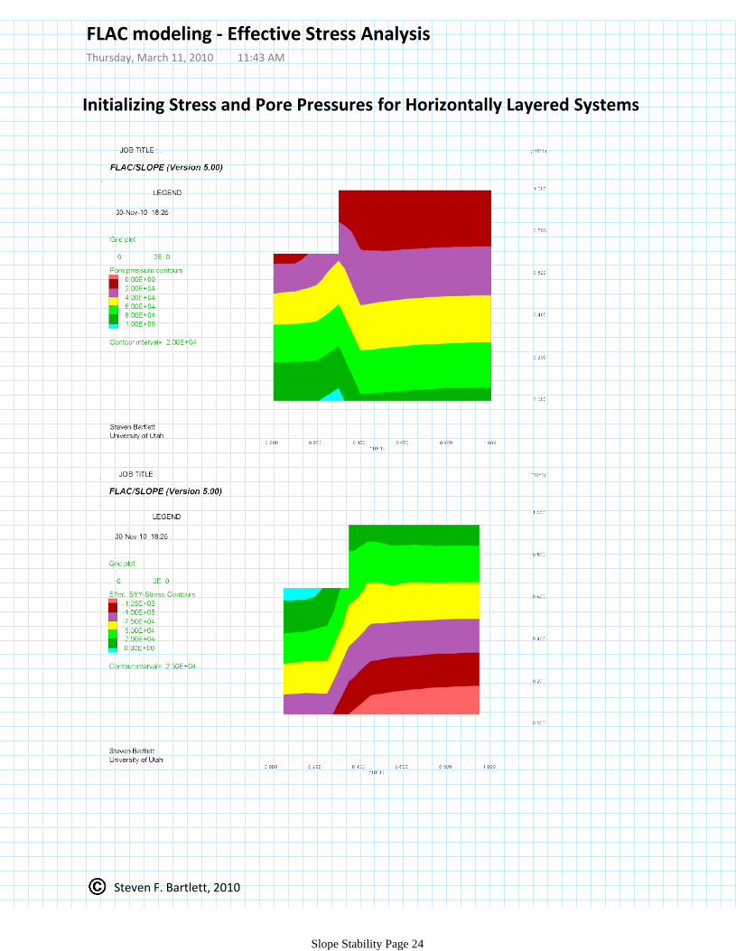
Initializing Stress and Pore Pressures for Horizontally Layered Systems

config gw ex=4g 10 10mo epro bulk 3e8 she 1e8 den 2000 por .4pro den 2300 por .3 j 3 5pro den 2500 por .2 j 1 2pro perm 1e-9mo null i=1,3 j=8,10water bulk 2e9 den 1000set g=9.8call iniv.fis; this file must be present in project file folderset k0=0.7i_stressfix x i 1fix x i 11fix y j 1hist unbalset flow offstep 1save iniv.savsolveretFLACsave initiate.sav 'last project state'

FLAC modeling - Effective Stress Analysis Thursday, March 11, 2010 11:43 AM



Initializing Stress and Pore Pressures for Horizontally Layered Systems

FLAC modeling - Effective Stress Analysis Thursday, March 11, 2010 11:43 AM



If a model containing interfaces is configured for groundwater flow, effective stresses (for the purposes of slip conditions) will be initialized along the interfaces (i.e., the presence of pore pressures will be accounted for within the interface stresses when stresses are initialized in the grid). To correctly account for pore pressures, CONFIG gw must be specified. For example, the WATER table command (in non-CONFIG gw mode) will not include pore pressures along the interface, because pore pressures are not defined at gridpoints for interpolation to interface nodes for this mode. Note that flow takes place, without resistance, from one surface to the other surface of an interface, if they are in contact. Flow along an interface (e.g., fracture flow) is not computed, and the mechanical effect of changing fluid pressure in an interface is not modeled. If the interface pore pressure is greater than the total stress acting across the interface (i.e., if the effective stress tends to be tensile), then the effective stress is set to zero for the purpose of calculating slip conditions.

FLAC modeling - Interface ConsiderationsThursday, March 11, 2010 11:43 AM



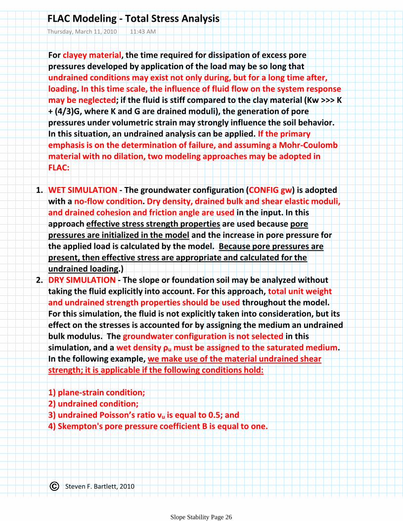
For clayey material, the time required for dissipation of excess pore pressures developed by application of the load may be so long that undrained conditions may exist not only during, but for a long time after, loading. In this time scale, the influence of fluid flow on the system response may be neglected; if the fluid is stiff compared to the clay material (Kw >>> K + (4/3)G, where K and G are drained moduli), the generation of pore pressures under volumetric strain may strongly influence the soil behavior. In this situation, an undrained analysis can be applied. If the primary emphasis is on the determination of failure, and assuming a Mohr-Coulomb material with no dilation, two modeling approaches may be adopted in FLAC:

WET SIMULATION - The groundwater configuration (CONFIG gw) is adopted with a no-flow condition. Dry density, drained bulk and shear elastic moduli, and drained cohesion and friction angle are used in the input. In this approach effective stress strength properties are used because pore pressures are initialized in the model and the increase in pore pressure for the applied load is calculated by the model. Because pore pressures are present, then effective stress are appropriate and calculated for the undrained loading.)

1.

DRY SIMULATION - The slope or foundation soil may be analyzed without taking the fluid explicitly into account. For this approach, total unit weight and undrained strength properties should be used throughout the model.

2.

For this simulation, the fluid is not explicitly taken into consideration, but its effect on the stresses is accounted for by assigning the medium an undrained bulk modulus. The groundwater configuration is not selected in this simulation, and a wet density ρu must be assigned to the saturated medium. In the following example, we make use of the material undrained shear strength; it is applicable if the following conditions hold:

1) plane-strain condition;2) undrained condition;3) undrained Poisson’s ratio νu is equal to 0.5; and4) Skempton's pore pressure coefficient B is equal to one.

FLAC Modeling - Total Stress AnalysisThursday, March 11, 2010 11:43 AM



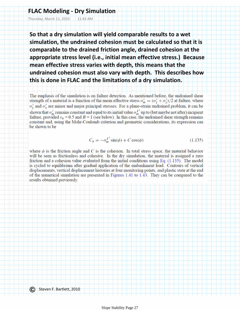
So that a dry simulation will yield comparable results to a wet simulation, the undrained cohesion must be calculated so that it is comparable to the drained friction angle, drained cohesion at the appropriate stress level (i.e., initial mean effective stress.) Because mean effective stress varies with depth, this means that the undrained cohesion must also vary with depth. This describes how this is done in FLAC and the limitations of a dry simulation.

FLAC Modeling - Dry SimulationThursday, March 11, 2010 11:43 AM



; WET SIMULATION ****config gw ex 5grid 20 10model mohrdef prop_valw_bu = 2e9 ; water bulk modulusd_po = 0.5 ; porosityd_bu = 2e6 ; drained bulk modulusd_sh = 1e6 ; shear modulusd_de = 1500 ; dry densityw_de = 1000 ; water densityb_mo = w_bu / d_po ; Biot modulus, Md_fr = 25.0 ; frictiond_co = 5e3 ; cohesionendprop_val;ini x mul 2prop dens=d_de sh=d_sh bu=d_bu; drained propertiesprop poros=d_po fric=d_fr coh=d_co tens 1e20water dens=w_de bulk=w_bu tens=1e30set grav=10; --- boundary conditions ---fix x i=1fix x i=21fix x y j=1; --- initial conditions ---ini syy -2e5 var 0 2e5ini sxx -1.5e5 var 0 1.5e5ini szz -1.5e5 var 0 1.5e5ini pp 1e5 var 0 -1e5set flow=off;; --- surcharge from embankment ---def ramp ramp = min(1.0,float(step)/4000.0)endapply syy=0 var -5e4 0 his ramp i=5,8 j=11apply syy=-5e4 var 5e4 0 his ramp i=8,11 j=11;; --- histories ---his nstep 100his ydisp i=2 j=9his ydisp i=8 j=9his ydisp i=8 j=6his ydisp i=8 j=3; --- run ---solvesave wet.sav

Undrained Analysis - Wet SimulationThursday, March 11, 2010 11:43 AM



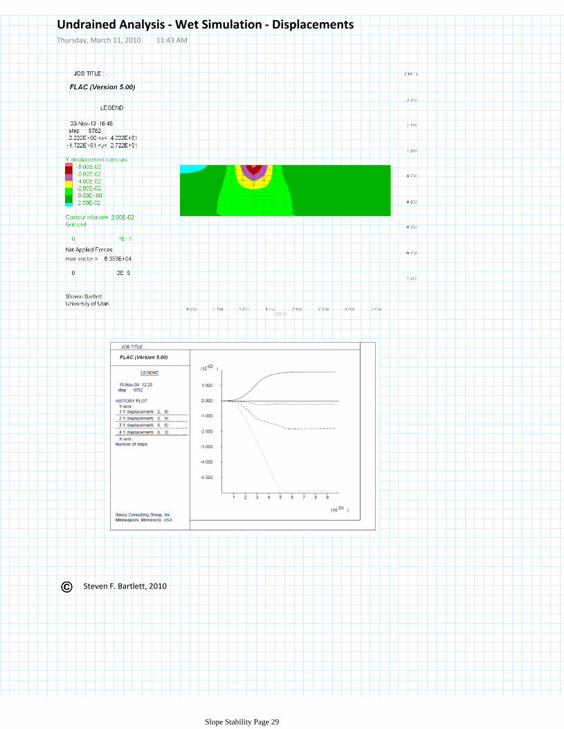
Undrained Analysis - Wet Simulation - DisplacementsThursday, March 11, 2010 11:43 AM



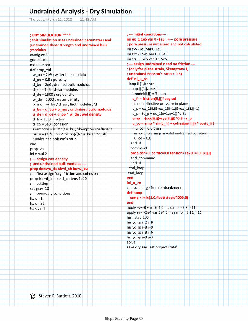
; DRY SIMULATION ****; this simulation uses undrained parameters and;undrained shear strength and undrained bulk;modulusconfig ex 5grid 20 10model mohrdef prop_val w_bu = 2e9 ; water bulk modulus d_po = 0.5 ; porosity d_bu = 2e6 ; drained bulk modulus d_sh = 1e6 ; shear modulus d_de = 1500 ; dry density w_de = 1000 ; water density b_mo = w_bu / d_po ; Biot modulus, M u_bu = d_bu + b_mo ; undrained bulk modulus u_de = d_de + d_po * w_de ; wet density d_fr = 25.0 ; friction d_co = 5e3 ; cohesion skempton = b_mo / u_bu ; Skempton coefficient nu_u = (3.*u_bu-2.*d_sh)/(6.*u_bu+2.*d_sh) ; undrained poisson’s ratioendprop_valini x mul 2; --- assign wet density; and undrained bulk modulus ---prop dens=u_de sh=d_sh bu=u_bu; --- first assign ’dry’ friction and cohesion prop fric=d_fr coh=d_co tens 1e20; --- setting ---set grav=10; --- boundary conditions ---fix x i=1fix x i=21fix x y j=1

; --- initial conditions ---ini ex_1 1e5 var 0 -1e5 ; <--- pore pressure; pore pressure initialized and not calculatedini syy -2e5 var 0 2e5ini sxx -1.5e5 var 0 1.5e5ini szz -1.5e5 var 0 1.5e5; --- assign undrained c and no friction ---; (only for plane strain, Skempton=1,; undrained Poisson’s ratio = 0.5)def ini_u_co loop ii (1,izones) loop jj (1,jzones) if model(ii,jj) = 3 then c_fr = friction(ii,jj)*degrad ; mean effective pressure in plane c_p = ex_1(ii,jj)+ex_1(ii+1,jj)+ex_1(ii,jj+1) c_p = (c_p + ex_1(ii+1,jj+1))*0.25 emp = -(sxx(ii,jj)+syy(ii,jj))*0.5 - c_p u_co = emp * sin(c_fr) + cohesion(ii,jj) * cos(c_fr) if u_co < 0.0 then iii=out(’ warning: invalid undrained cohesion’) u_co = 0.0 end_if command prop coh=u_co fric=0.0 tension=1e20 i=ii,ii j=jj,jj end_command end_if end_loopend_loop

endini_u_co; --- surcharge from embankment ---def ramp ramp = min(1.0,float(step)/4000.0)endapply syy=0 var -5e4 0 his ramp i=5,8 j=11apply syy=-5e4 var 5e4 0 his ramp i=8,11 j=11his nstep 100his ydisp i=2 j=9his ydisp i=8 j=9his ydisp i=8 j=6his ydisp i=8 j=3solvesave dry.sav 'last project state'

Undrained Analysis - Dry SimulationThursday, March 11, 2010 11:43 AM



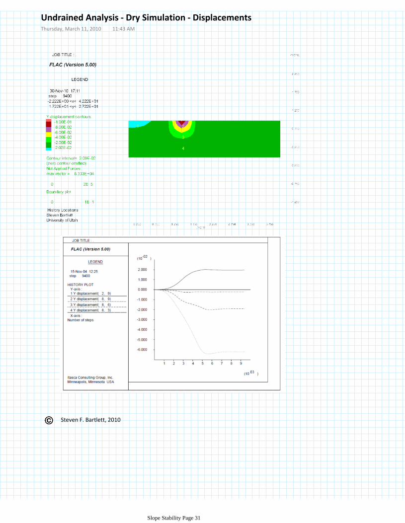
Undrained Analysis - Dry Simulation - DisplacementsThursday, March 11, 2010 11:43 AM



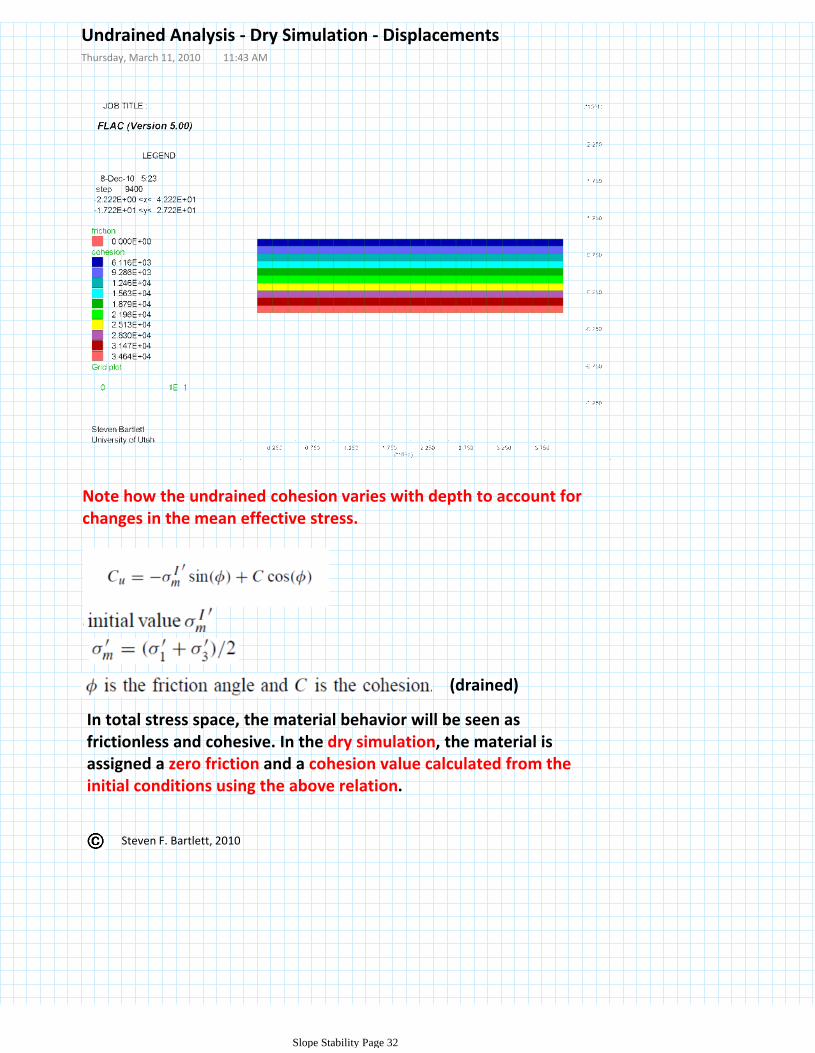
Note how the undrained cohesion varies with depth to account for changes in the mean effective stress.

(drained)

In total stress space, the material behavior will be seen as frictionless and cohesive. In the dry simulation, the material is assigned a zero friction and a cohesion value calculated from the initial conditions using the above relation.

Undrained Analysis - Dry Simulation - DisplacementsThursday, March 11, 2010 11:43 AM



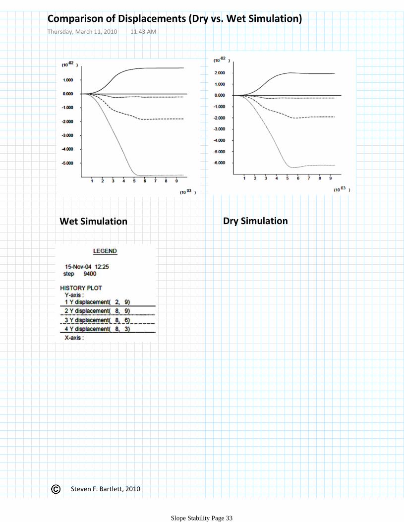
Wet Simulation Dry Simulation

Comparison of Displacements (Dry vs. Wet Simulation)Thursday, March 11, 2010 11:43 AM



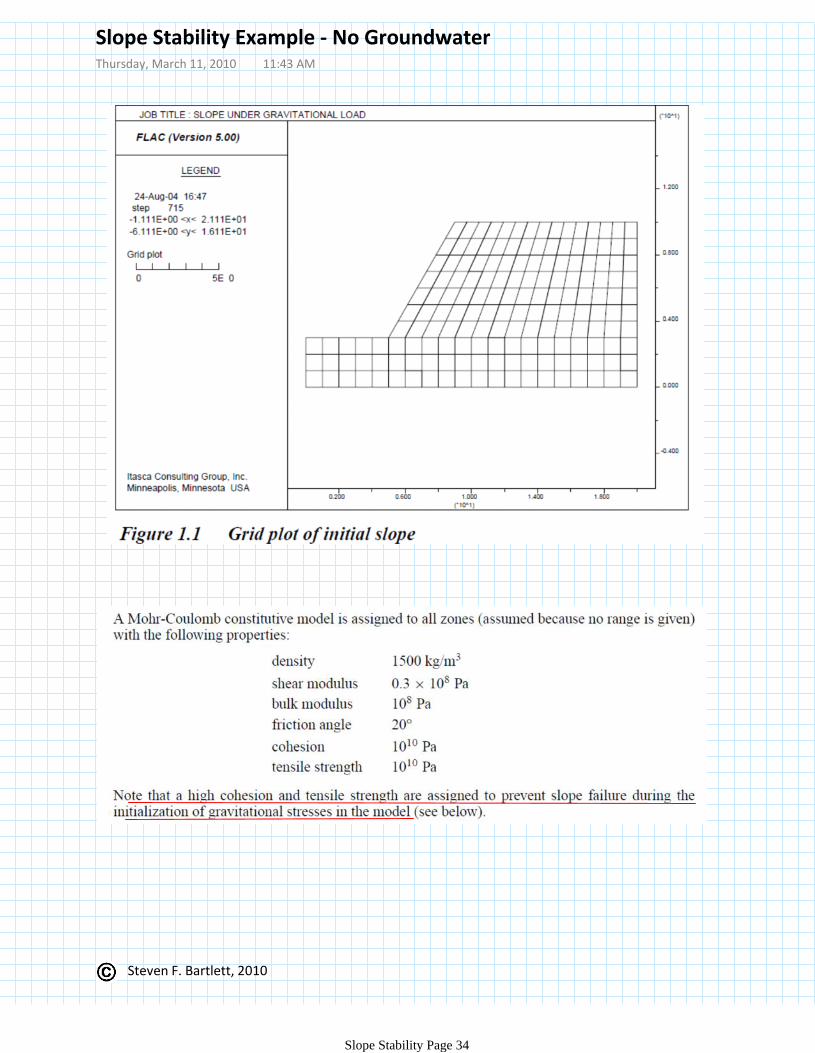
Slope Stability Example - No Groundwater Thursday, March 11, 2010 11:43 AM



Generating the slope

Slope Stability - No Groundwater (cont.)Thursday, March 11, 2010 11:43 AM



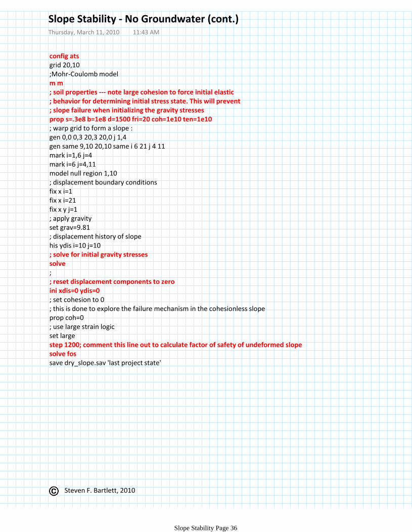
config atsgrid 20,10;Mohr-Coulomb modelm m; soil properties --- note large cohesion to force initial elastic; behavior for determining initial stress state. This will prevent; slope failure when initializing the gravity stressesprop s=.3e8 b=1e8 d=1500 fri=20 coh=1e10 ten=1e10; warp grid to form a slope :gen 0,0 0,3 20,3 20,0 j 1,4gen same 9,10 20,10 same i 6 21 j 4 11mark i=1,6 j=4mark i=6 j=4,11model null region 1,10; displacement boundary conditionsfix x i=1fix x i=21fix x y j=1; apply gravityset grav=9.81; displacement history of slopehis ydis i=10 j=10; solve for initial gravity stressessolve;; reset displacement components to zeroini xdis=0 ydis=0; set cohesion to 0; this is done to explore the failure mechanism in the cohesionless slopeprop coh=0; use large strain logicset largestep 1200; comment this line out to calculate factor of safety of undeformed slopesolve fossave dry_slope.sav 'last project state'




At step 1200

Factor of safety = 0.27 (However, this is surficial slip is not of particular interest. This slip surface will be eliminated, see next page. )




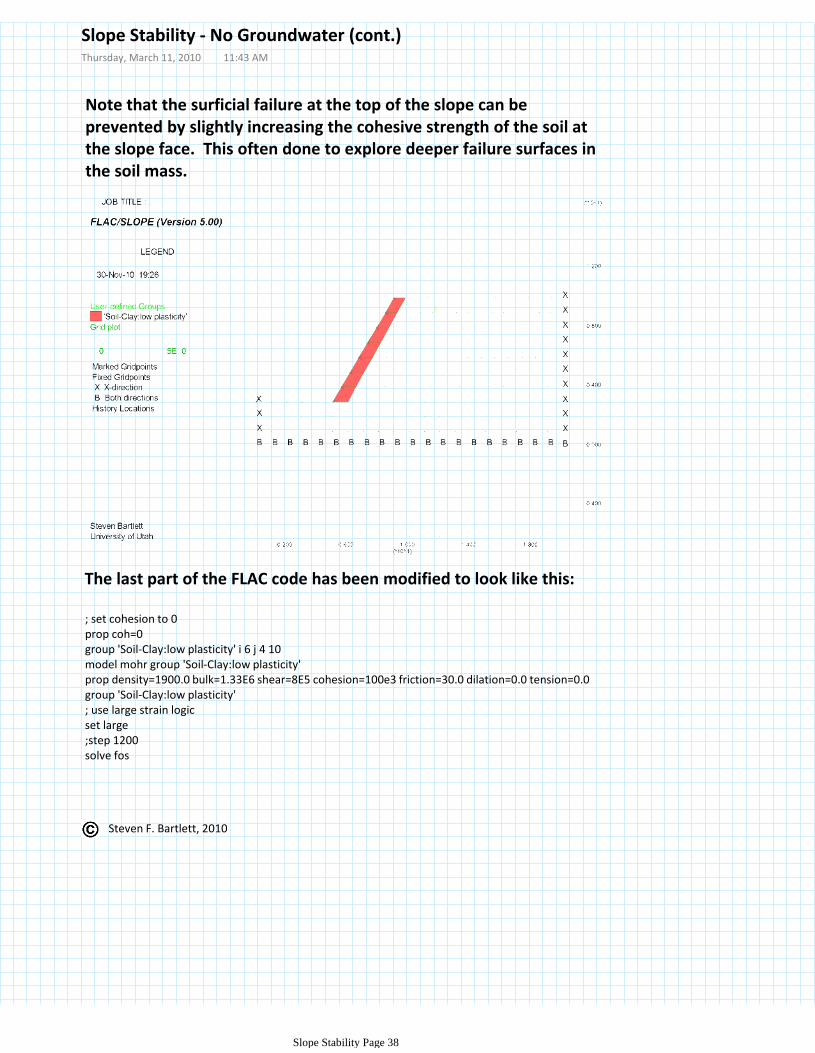
Note that the surficial failure at the top of the slope can be prevented by slightly increasing the cohesive strength of the soil at the slope face. This often done to explore deeper failure surfaces in the soil mass.

The last part of the FLAC code has been modified to look like this:

; set cohesion to 0prop coh=0group 'Soil-Clay:low plasticity' i 6 j 4 10 model mohr group 'Soil-Clay:low plasticity' prop density=1900.0 bulk=1.33E6 shear=8E5 cohesion=100e3 friction=30.0 dilation=0.0 tension=0.0 group 'Soil-Clay:low plasticity'; use large strain logicset large;step 1200solve fos




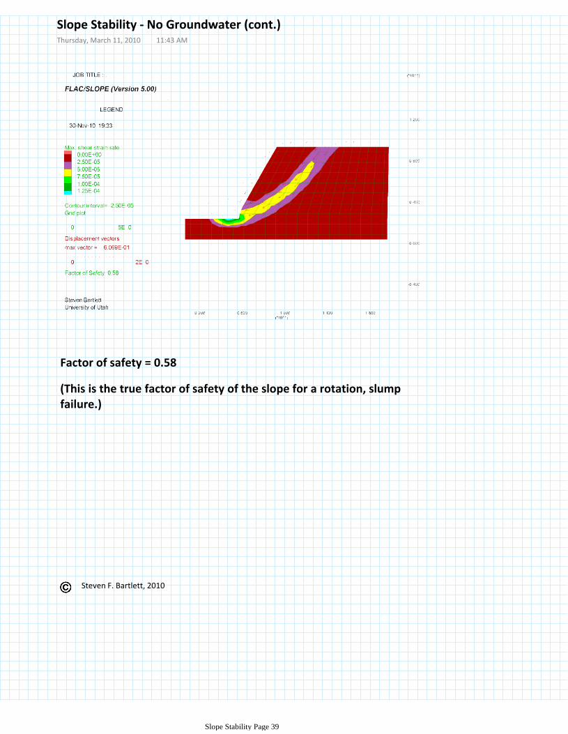
Factor of safety = 0.58

(This is the true factor of safety of the slope for a rotation, slump failure.)




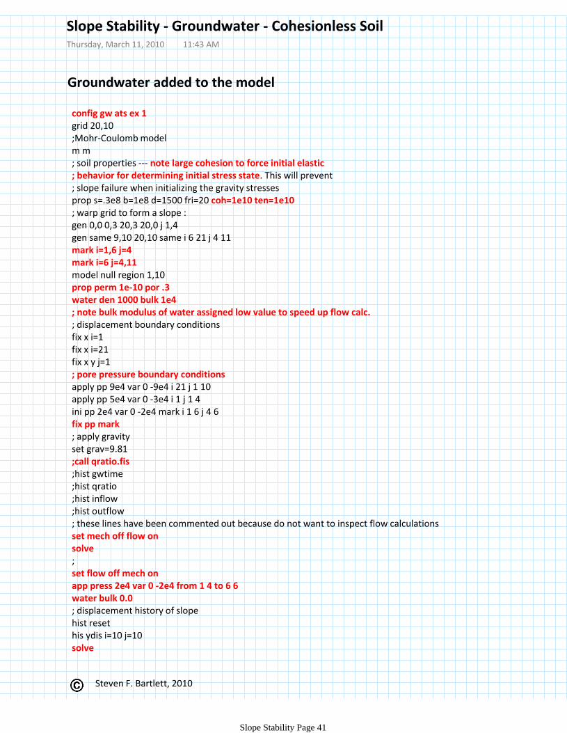
The groundwater flow option in FLAC can be used to find the phreatic surface and establish the pore pressure distribution before the mechanical response is investigated. The model is run in groundwater flow mode by using the CONFIG gw command.

We turn off the mechanical calculation (SET mech off) in order to establish the initial pore pressure distribution. We apply pore pressure boundary conditions to raise the water level to 5 m at the left boundary, and 9 m at the right. The slope is initially dry (INIsat 0). We also set the bulk modulus of the water to a low value (1.0 × 104) because our objective is to reach the steady-flow state as quickly as possible. The groundwater time scale is wrong in thiscase, but we are not interested in the transient time response. The steady-flow state is determined by using the SOLVE ratio command. When the groundwater flow ratio falls below the set value of 0.01,steady-state flow is achieved.

Mechanical equilibrium is then established including the pore pressure by turning flow off and mechanical on. These commands turn off the flow calculation, turn on the mechanical calculation, apply the weight of the water to the slope surface, and set the bulk modulus of the water to zero. This last command also prevents pore pressures from generating as a result of mechanical deformation.

Slope Stability - Groundwater - Cohesionless SoilThursday, March 11, 2010 11:43 AM



config gw ats ex 1grid 20,10;Mohr-Coulomb modelm m; soil properties --- note large cohesion to force initial elastic; behavior for determining initial stress state. This will prevent; slope failure when initializing the gravity stressesprop s=.3e8 b=1e8 d=1500 fri=20 coh=1e10 ten=1e10; warp grid to form a slope :gen 0,0 0,3 20,3 20,0 j 1,4gen same 9,10 20,10 same i 6 21 j 4 11mark i=1,6 j=4mark i=6 j=4,11model null region 1,10prop perm 1e-10 por .3water den 1000 bulk 1e4; note bulk modulus of water assigned low value to speed up flow calc.; displacement boundary conditionsfix x i=1fix x i=21fix x y j=1; pore pressure boundary conditionsapply pp 9e4 var 0 -9e4 i 21 j 1 10apply pp 5e4 var 0 -3e4 i 1 j 1 4ini pp 2e4 var 0 -2e4 mark i 1 6 j 4 6fix pp mark; apply gravityset grav=9.81;call qratio.fis;hist gwtime;hist qratio;hist inflow;hist outflow; these lines have been commented out because do not want to inspect flow calculationsset mech off flow onsolve;set flow off mech onapp press 2e4 var 0 -2e4 from 1 4 to 6 6water bulk 0.0; displacement history of slopehist resethis ydis i=10 j=10solve

Groundwater added to the model




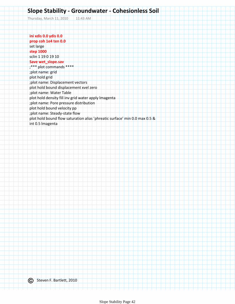
ini xdis 0.0 ydis 0.0prop coh 1e4 ten 0.0set largestep 1000sclin 1 19 0 19 10Save wet_slope.sav ;*** plot commands ****;plot name: gridplot hold grid;plot name: Displacement vectorsplot hold bound displacement xvel zero;plot name: Water Tableplot hold density fill inv grid water apply lmagenta;plot name: Pore pressure distributionplot hold bound velocity pp;plot name: Steady-state flowplot hold bound flow saturation alias ’phreatic surface’ min 0.0 max 0.5 &int 0.5 lmagenta



Displacement vectors and X-velocity contours




Pore pressure distribution and displacement vectors



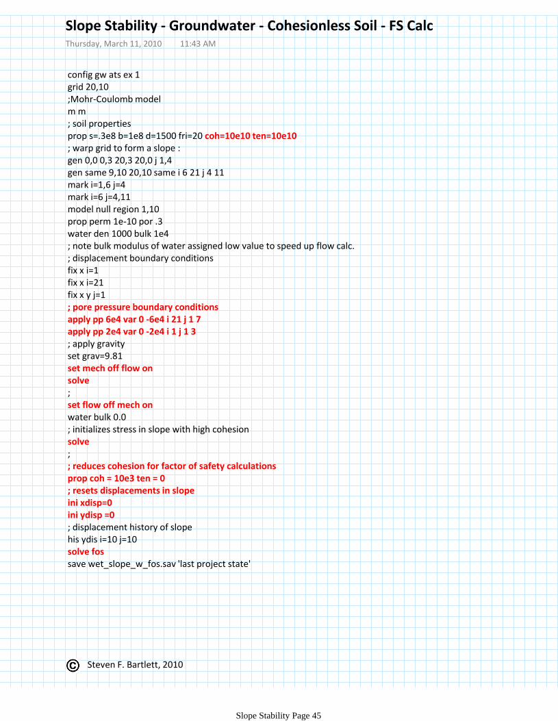
config gw ats ex 1grid 20,10;Mohr-Coulomb modelm m; soil propertiesprop s=.3e8 b=1e8 d=1500 fri=20 coh=10e10 ten=10e10; warp grid to form a slope :gen 0,0 0,3 20,3 20,0 j 1,4gen same 9,10 20,10 same i 6 21 j 4 11mark i=1,6 j=4mark i=6 j=4,11model null region 1,10prop perm 1e-10 por .3water den 1000 bulk 1e4; note bulk modulus of water assigned low value to speed up flow calc.; displacement boundary conditionsfix x i=1fix x i=21fix x y j=1; pore pressure boundary conditionsapply pp 6e4 var 0 -6e4 i 21 j 1 7apply pp 2e4 var 0 -2e4 i 1 j 1 3; apply gravityset grav=9.81set mech off flow onsolve;set flow off mech onwater bulk 0.0; initializes stress in slope with high cohesionsolve;; reduces cohesion for factor of safety calculationsprop coh = 10e3 ten = 0; resets displacements in slopeini xdisp=0ini ydisp =0; displacement history of slopehis ydis i=10 j=10solve fossave wet_slope_w_fos.sav 'last project state'

Slope Stability - Groundwater - Cohesionless Soil - FS CalcThursday, March 11, 2010 11:43 AM



Slope Stability - Groundwater - Cohesionless Soil - FS CalcThursday, March 11, 2010 11:43 AM



BlankThursday, March 11, 2010 11:43 AM


Documents

Slope and Embankment Stability - Civil Engineeringbartlett/CVEEN5305/Slope Stability… · · 2015-12-12Slope and Embankment Stability Thursday, March 11, 2010 11:43 AM Slope Stability