Slice Sampling on Hamiltonian Trajectories

Benjamin Bloem-Reddy REDDY@STAT.COLUMBIA.EDUJohn P. Cunningham JPC2181@COLUMBIA.EDU

Department of Statistics, Columbia University

AbstractHamiltonian Monte Carlo and slice samplingare amongst the most widely used and stud-ied classes of Markov Chain Monte Carlo sam-plers. We connect these two methods and presentHamiltonian slice sampling, which allows slicesampling to be carried out along Hamiltoniantrajectories, or transformations thereof. Hamil-tonian slice sampling clarifies a class of modelpriors that induce closed-form slice samplers.More pragmatically, inheriting properties of slicesamplers, it offers advantages over HamiltonianMonte Carlo, in that it has fewer tunable hyper-parameters and does not require gradient infor-mation. We demonstrate the utility of Hamil-tonian slice sampling out of the box on prob-lems ranging from Gaussian process regressionto Pitman-Yor based mixture models.

1. IntroductionAfter decades of work in approximate inference and nu-merical integration, Markov Chain Monte Carlo (MCMC)techniques remain the gold standard for working with in-tractable probabilistic models, throughout statistics andmachine learning. Of course, this gold standard alsocomes with sometimes severe computational requirements,which has spurred many developments for increasing theefficacy of MCMC. Accordingly, numerous MCMC algo-rithms have been proposed in different fields and with dif-ferent motivations, and perhaps as a result the similaritiesbetween some popular methods have not been highlightedor exploited. Here we consider two important classes ofMCMC methods: Hamiltonian Monte Carlo (HMC) (Neal,2011) and slice sampling (Neal, 2003).

HMC considers the (negative log) probability of the in-tractable distribution as the potential energy of a Hamil-

Proceedings of the 33 rd International Conference on MachineLearning, New York, NY, USA, 2016. JMLR: W&CP volume48. Copyright 2016 by the author(s).

tonian system, and samples a new point from the distribu-tion by simulating a dynamical trajectory from the currentsample point. With careful tuning, HMC exhibits favorablemixing properties in many situations, particularly in highdimensions, due to its ability to take large steps in sam-ple space if the dynamics are simulated for long enough.Proper tuning of HMC parameters can be difficult, andthere has been much interest in automating it; examples in-clude Wang et al. (2013); Hoffman & Gelman (2014). Fur-thermore, better mixing rates associated with longer trajec-tories can be computationally expensive because each sim-ulation step requires an evaluation or numerical approxi-mation of the gradient of the distribution.

Similar in objective but different in approach is slice sam-pling, which attempts to sample uniformly from the volumeunder the target density. Slice sampling has been employedsuccessfully in a wide range of inference problems, in largepart because of its flexibility and relative ease of tuning(very few if any tunable parameters). Although efficientlyslice sampling from univariate distributions is straightfor-ward, in higher dimensions it is more difficult. Previous ap-proaches include slice sampling each dimension individu-ally, amongst others. One particularly successful approachis to generate a curve, parameterized by a single scalarvalue, through the high-dimensional sample space. Ellip-tical slice sampling (ESS) (Murray et al., 2010) is one suchapproach, generating ellipses parameterized by θ ∈ [0, 2π].As we show in section 2.2, ESS is a special case of ourproposed sampling algorithm.

In this paper, we explore the connections between HMCand slice sampling by observing that the elliptical trajectoryused in ESS is the Hamiltonian flow of a Gaussian poten-tial. This observation is perhaps not surprising – indeed itappears at least implicitly in Neal (2011); Pakman & Panin-ski (2013); Strathmann et al. (2015) – but here we leveragethat observation in a way not previously considered. To wit,this connection between HMC and ESS suggests that wemight perform slice sampling along more general Hamil-tonian trajectories, a method we introduce under the nameHamiltonian slice sampling (HSS). HSS is of theoretical in-terest, allowing us to consider model priors that will induce

Slice Sampling on Hamiltonian Trajectories

simple closed form slice samplers. Perhaps more impor-tantly, HSS is of practical utility. As the conceptual off-spring of HMC and slice sampling, it inherits the relativelysmall amount of required tuning from ESS and the abilityto take large steps in sample space from HMC techniques.

In particular, we offer the following contributions:

• We clarify the link between two popular classes ofMCMC techniques.

• We introduce Hamiltonian slice sampling, a generalsampler for target distributions that factor into twocomponents (e.g., a prior and likelihood), where theprior factorizes or can be transformed so as to factor-ize, and all dependence structure in the target distri-bution is induced by the likelihood or the intermediatetransformation.

• We show that the prior can be either of a form whichinduces analytical Hamiltonian trajectories, or moregenerally, of a form such that we can derive such a tra-jectory via a measure preserving transformation. No-table members of this class include Gaussian processand stick-breaking priors.

• We demonstrate the usefulness of HSS on a range ofmodels, both parametric and nonparametric.

We first review HMC and ESS to establish notation and aconceptual framework. We then introduce HSS generally,followed by a specific version based on a transformation tothe unit interval. Finally, we demonstrate the effectivenessand flexibility of HSS on two different popular probabilisticmodels.

2. Sampling via Hamiltonian dynamicsWe are interested in the problem of generating samples ofa random variable f from an intractable distribution π∗(f),either directly or via a measure preserving transformationr−1(q) = f . For clarity, we use f to denote the quantityof interest in its natural space as defined by the distributionπ∗, and q denotes the transformed quantity of interest inHamiltonian phase space, as described in detail below. Wedefer further discussion of the map r(·) until section 2.4,but note that in typical implementations of HMC and ESS,r(·) is the indentity map, i.e. f = q.

2.1. Hamiltonian Monte Carlo

HMC generates MCMC samples from a target dis-tribution, often an intractable posterior distribution,π∗(q) := 1

Z π(q), with normalizing constant Z, by simu-lating the Hamiltonian dynamics of a particle in the poten-tial U(q) = − log π(q). We are free to specify a distribu-tion for the particle’s starting momentum p, given which

the system evolves deterministically in an augmented statespace (q,p) according to Hamilton’s equations. In par-ticular, at the i-th sampling iteration of HMC, the initialconditions of the system are q0 = q(i−1), the previoussample, and p0, which in most implementations is sam-pled from N (0,M). M is a “mass” matrix that may beused to express a priori beliefs about the scaling and depen-dence of the different dimensions, and for models with highdependence between sampling dimensions, M can greatlyaffect sampling efficiency. An active area of research isinvestigating how to adapt M for increased sampling effi-ciency; for example Girolami & Calderhead (2011); Betan-court et al. (2016). For simplicity, in this work we assumethroughout that M is set ahead of time and remains fixed.The resulting Hamiltonian is

H(q,p) = − log π(q) +1

2pTM−1p. (1)

When solved exactly, Hamilton’s equations generateMetropolis-Hastings (MH) proposals that are accepted withprobability 1. In most situations of interest, Hamilton’sequations do not have an analytic solution, so HMC is of-ten performed using a numerical integrator, e.g. Störmer-Verlet, which is sensitive to tuning and can be computation-ally expensive due to evaluation or numerical approxima-tion of the gradient at each step. See Neal (2011) for moredetails.

2.2. Univariate and Elliptical Slice Sampling

Univariate slice sampling (Neal, 2003) generates samplesuniformly from the area beneath a density p(x), such thatthe resulting samples are distributed according to p(x).It proceeds as follows: given a sample x0, a thresholdh ∼ U(0, p(x0)) is sampled; the next sample x1 is thensampled uniformly from the slice S := {x : p(x) > h}.When S is not known in closed form, a proxy slice S′ canbe randomly constructed from operations that leave the uni-form distribution on S invariant. In this paper, we use thestepping out and shrinkage procedure, with parameters w,the width, and m, the step out limit, from Neal (2003).

ESS (Murray et al., 2010) is a popular sampling algorithmfor latent Gaussian models, e.g., Markov random field orGaussian process (GP) models. For a latent multivariateGaussian f ∈ Rd with prior π(f) = N (f |0,Σ), ESS gen-erates MCMC transitions f → f ′ by sampling an auxiliaryvariable ν ∼ N (0,Σ) and slice sampling the likelihoodsupported on the ellipse defined by

f ′ = f cos θ + ν sin θ, θ ∈ [0, 2π]. (2)

Noting the fact that the solutions to Hamilton’s equations inan elliptical potential are ellipses, we may reinterpret ESS.The Hamiltonian induced by π(q) ∝ N (q|0,Σ) and mo-

Slice Sampling on Hamiltonian Trajectories

mentum distribution p ∼ N (0,M) is

H(q,p) =1

2qTΣ−1q +

1

2pTM−1p. (3)

WhenM = Σ−1, Hamilton’s equations yield the trajectory

q(t) = q(0) cos t+ Σp(0) sin t, t ∈ (−∞,∞), (4)

which is an ellipse. Letting r(·) be the identity map, andq(0) be the value of f from the previous iteration of anMCMC sampler, the trajectories of possible sample valuesgiven by (2) and (4) are distributionally equivalent withθ = t mod 2π because ν

d= Σp(0) = M−1p(0). The

ESS variable ν thus takes on the interpretation of the ini-tial velocity of the particle. Accordingly, we have clarifiedthe link between HMC and ESS. The natural next questionis what this observation offers in terms of a more generalsampling strategy.

2.3. Hamiltonian Slice Sampling

Using the connection between HMC and ESS, we pro-pose the sampling algorithm given in Algorithm 1, calledHamiltonian slice sampling (HSS). The idea of HSS isthe same as ESS: use the prior distribution to generate ananalytic curve through sample space, then slice sample onthe curve according to the likelihood in order to generate asample from the posterior distribution. In the special distri-butions for which Hamilton’s equations have analytic solu-tions and the resulting trajectories can be computed exactly,e.g. the multivariate Gaussian distribution, the trajectorieshave a single parameter, t ∈ (−∞,∞). This simple param-eterization is crucial: it enables us to use univariate slicesampling methods (Neal, 2003) in higher dimensions. Theadvantage of univariate slice sampling techniques is thatthey require little tuning; the slice width adapts to the dis-tribution and sampler performance does not depend greatlyon the sampler parameters.

We include in the Supplementary Materials some examplesof distributions for which Hamilton’s equations have ana-lytical solutions. However, these special cases are in theminority, and most distributions do not admit analytic solu-tions. In such a case, a measure preserving transformationto a distribution that does have analytic solutions is nec-essary. Let r(·) denote such a transformation. We deferelaboration on specific transformations until the followingsection, but it is sufficient for r(·) to be differentiable andone-to-one. In particular, we will make extensive use of theinverse function r−1(·).

We next show that Algorithm 1 is a valid MCMC samplerfor a target distribution π∗(f |D) = 1

ZL(D|f) π(f). Theproof of validity is conceptually so similar to ESS that theproof in Murray et al. (2010) nearly suffices. For complete-ness, we here show that the dynamics used to generate new

Algorithm 1 Hamiltonian slice sampling

Input: Current state f ; differentiable, one-to-one trans-formation q := r(f) with Jacobian J(r−1(q))Output: A new state f ′. If f is drawn from π∗, themarginal distribution of f ′ is also π∗.

1: Sample momentum for each component of q:

p ∼ N (0,M)

2: Obtain analytic solution q′(t) to Hamilton’s equations,where p0 = p and q′0 = q

3: Set slice sampling threshold:

u ∼U[0, 1]

log h← logL(D|f)− log |J(r−1(q))|+ log u

4: Slice sample along r−1(q′(t)) for t∗ ∈ (−∞,∞), us-ing the methods of (Neal, 2003) and threshold h on:

log π∗(f ′|f ,p,D, u, t) ∝logL(D|f ′(t))− log |J(r−1(q(t)))| (5)

5: return f ′(t∗) = r−1(q′(t∗))

states are reversible, and as such, π∗ is a stationary distribu-tion of the Markov chain defined by Algorithm 1. Further-more, the sampler has non-zero probability of transitioningto any region that has non-zero probability under π∗. Takentogether, these facts clarify that the sampler will convergeto a unique stationary distribution that yields samples of fthat are marginally distributed according to the target π∗.

Consider the joint distribution of the random variablesin Algorithm 1 (suppressing hyperparameters for simplicityand denoting by {tk} the sequence of variables producedby the univariate slice sampling algorithm):

p(f ,p,h, {tk}) = π∗(f |D) p(p) p(h|f ,D) p({tk}|f ,p, h)

(6)

=1

ZL(D|f) π(f) p(p) p(h|f ,D) p({tk}|f ,p, h)

(7)

Now, remembering that for a differentiable, one-to-one transformation r(·), such that f = r−1(q),with Jacobian J(·), the density of q is given byπ(q) = π(r−1(q))|J(r−1(q))|. Combining this withthe density of the slice sampling threshold variable implied

Slice Sampling on Hamiltonian Trajectories

by step 3 of Algorithm 1, p(h|f ,D) = |J(r−1(q))|L(D|f) , we have

p(f ,p,h, {tk})

=1

ZL(D|f) π(r−1(q)) · |J(r−1(q))|

|J(r−1(q))|. . .

× p(p) p(h|f ,D) p({tk}|f ,p, h) (8)∝ π(q) p(p) p({tk}|q,p, h) (9)

Exact Hamiltonian dynamics for (q,p) are reversible,keeping constant the factor π(q) p(p), and they yield atrajectory in q-space parameterized by t that can be trans-formed into f -space as f(t) = r−1(q(t)). Given the Hamil-tonian trajectory, the univariate slice sampling methods,e.g. the step-out and shrinkage procedures from Neal(2003) can be applied to f(t); these, too, are reversible. Wetherefore have p(f ,p, h, {tk}) = p(f ′,p′, h, {t′k}) for anyf ′ generated by starting at f , which concludes the proof ofvalidity for HSS.

2.4. HSS via the Probability Integral Transformation

The multivariate Gaussian distribution is a special case forwhich Hamilton’s equations can be solved analytically, asdemonstrated by ESS. This fact forms the basis for Pak-man & Paninski (2013; 2014). The univariate uniform andexponential distributions also have analytic solutions. Inthe remainder of the paper, we focus on transformationsof uniform random variables; see the Supplementary Ma-terials for details on the exponential distribution and a fewrelated transformations.

Hamiltonian dynamics under the uniform distributionq ∼ U[0, 1] are the extremely simple billiard ball dynamics:the particle moves back and forth across the unit interval atconstant speed q0 = p0/m, reflecting off the boundaries ofthe interval. The relevant quantities are the initial reflectiontime,

R0 =|1{q0 > 0} − q0|

q0, (10)

where q0 is the initial velocity, and the period of a fulltraversal of the unit interval,

T =1

q0=m

p0. (11)

These simple dynamics can be used to construct analyticcurves on which to slice sample for any continuous priorwith computable inverse cumulative distribution function(CDF). In particular, for a random variable f with CDFG(f) and density g(f), the distribution of q := G(f) isU[0, 1]. The dynamics on the unit interval yield the trajec-tory q(t); the resulting curve is f(t) = G−1(q(t)). In thiscase the Jacobian is 1/g(f), so the slice sampling target

x1

x2

x1

x2

x1

x2

x1

x2

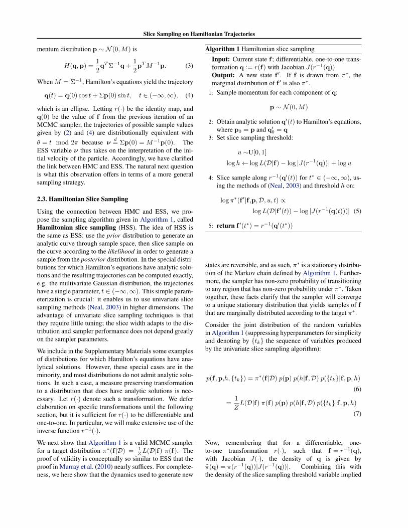
Figure 1. Example trajectories from HSS (top) and ESS (bottom).Yellow dots are starting points, blue dots are end points of Hamil-tonian trajectories. Top left: Uniform trajectory in two indepen-dent dimensions. Top right: The resulting bivariate normal HSStrajectory via the probability integral transformation. Bottom left:Elliptical trajectory in two dimensions. The green dot in is ν fromESS. Bottom right: Transformation of the elliptical trajectory tothe unit square.

in Equation 5 of Algorithm 1 is exactly proportional to theposterior.

Although f(t) is not a Hamiltonian flow in sample space,it is a measure preserving transformation of a Hamiltonianflow in the unit hypercube, and so preserves sampling va-lidity. For the remainder of the paper, we use transforma-tions to uniform random variables, and we refer to the re-sulting sampler as HSS. We note, however that it is onlyone instantiation of the general class of Hamiltonian slicesampling methods: any suitable transformation would pro-duce different resulting dynamics in sample space.

Using this or any other transformation in Algorithm 1 gen-erates curves through sample space only using informationfrom the prior and the transformation. A useful line of in-quiry is whether we can adapt the transformation or theprior to sample more efficiently. The problem of choos-ing or adapting to a prior that better captures the poste-rior geometry of the sample space is shared by all sam-plers based on Hamiltonian dynamics, including ESS andHMC. The issue is explored in depth in Girolami & Calder-head (2011); Betancourt et al. (2016). A possible approachto making the prior more flexible is via a pseudo-prior, asin Nishihara et al. (2014); Fagan et al. (2016). We do notexplore such an approach here, but note that a pseudo-priorcould be incorporated easily in Algorithm 1.

The basic requirement that must be satisfied in order tomake our method applicable is that some component of the

Slice Sampling on Hamiltonian Trajectories

target distribution can be expressed as a collection of con-ditionally independent variables. This is often the case inhierarchical Baysian models, as in section 3.2. As a sim-ple example, whitening a collection of multivariate Gaus-sian random variables induces independence, enabling thesimulation of independent uniform dynamics. An exampleof such dynamics on the unit square, along with the result-ing trajectory in two-dimensional Gaussian space, is shownin Figure 1. For comparison, Figure 1 also shows an exam-ple ESS trajectory from the same distribution, along withits transformation to the unit square.

In principle, the HSS trajectory has access to different, pos-sibly larger, regions of the sample space, as it is not con-strained to a closed elliptical curve. It also spends rela-tively more time in regions of higher prior probability, asthe particle’s velocity in the original space is inversely pro-portional to the the prior density, i.e. f(t) = q0/g(f), aswill be illustrated in section 3.2. This behavior also sug-gests that if the prior is sharply concentrated on some re-gion, the sampler may get stuck. In order to avoid patholo-gies, relatively flat priors should be used. If the prior hyper-parameters are also to be sampled, it should be done suchthat they make small moves relative to the parameters sam-pled by HSS. See Neal (2011, section 5.4.5) for discussionon this point in the context of HMC.

2.5. Related Work

HSS slice samples on a trajectory calculated using Hamil-tonian dynamics. A similar idea underlies the No U-TurnSampler (NUTS) (Hoffman & Gelman, 2014), which slicesamples from the discrete set of states generated by the nu-merical simulation of Hamiltonian dynamics induced bythe posterior distribution of interest. Other methods of mul-tivariate slice sampling include those given in Neal (2003).Most often, each variable is slice sampled separately, whichcan lead to the same convergence problems as Gibbs sam-pling when the variables are highly dependent. Murrayet al. (2010) review other sampling methods for latent GPmodels, of which HSS is another example. In so much aswe derived HSS by noticing connections between existingmethods, other commonalities may indeed exist.

ESS also fits into the framework of the preconditionedCrank-Nicholson (pCN) proposals studied in, e.g., Cotteret al. (2013). As those authors point out, the pCN pro-posal is a generalization of a random walk in the samplespace, where “the target measure is defined with respect toa Gaussian.” HSS also fits in this framework, with the tar-get measure π∗ defined with respect to non-Gaussian den-sities. ESS and HSS, like pCN, are dimension-free meth-ods; their statistical efficiency is independent of the dimen-sion of the sample space (Hairer et al., 2014). However,as more data is observed, and the posterior moves further

x2907 x 359 x 164EffectiveSamples

0

1ESS σp = 0.1 σp = 0.25

x134 x140 x142

CPU

Tim

e(s)

0

2

4

Dimension1 5 10

LhoodEvals

(M)

0

1

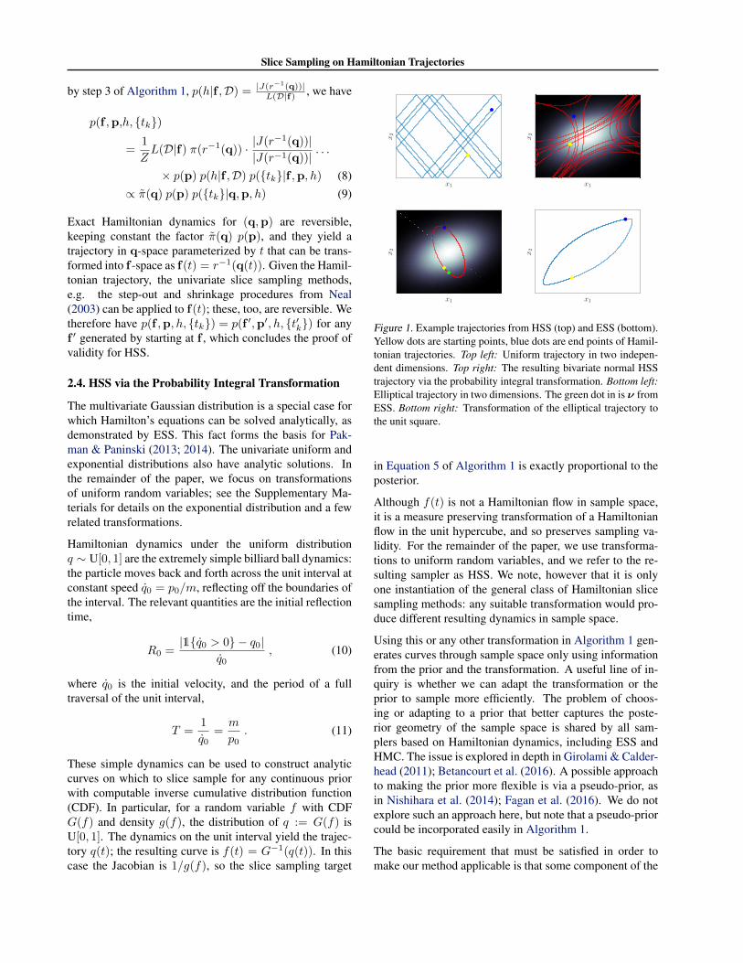
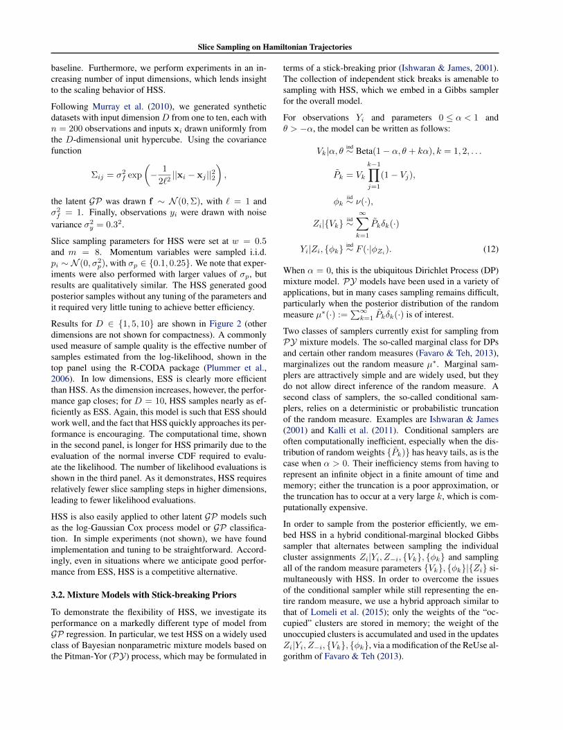
Figure 2. Effective number of samples for ESS and HSS from 105

iterations after 104 burn in on GP regression, averaged across50 experiments. σp denotes the standard deviation of the normaldistribution from which the Hamiltonian momentum variable pis sampled. Top: Effective samples. Middle: Evaluation time.Bottom: Number of likelihood evaluations.

from the prior, sampler performance may degrade – hencethe motivation for adaptive techniques such as Nishiharaet al. (2014); Fagan et al. (2016). Extending HSS to in-clude pseudo-priors or Metropolis-adjusted Langevin-typevariations, as in Cotter et al. (2013), is an interesting direc-tion for future work.

3. ExperimentsIn order to test the effectiveness and flexibility of HSS,we performed experiments on two very different models.The first is latent GP regression on synthetic data, whichallows us to make a direct comparison between HSS andESS. The second is a non-parametric mixture of Gaussianswith a stick-breaking prior, which demonstrates the flexi-bility of HSS. In both, we use the step-out and shrinkageslice sampling methods. See Neal (2003) for details.

3.1. GP Regression

We consider the standard GP regression model. We as-sume a latent GP f over an input space X . Noisy Gaussianobservations y = {y1, ..., yn} are observed at locations{x1, ...,xn}, and observations are conditionally indepen-dent with likelihood L(D|f) :=

∏ni=1N (yi|f(xi), σ

2y),

where σ2y is the variance of the observation noise. Al-

though the posterior is conjugate and can be sampled inclosed form, the simplicity of the model allows us to testthe performance of HSS against that of ESS on a model forwhich ESS is ideally suited, forming a highly conservative

Slice Sampling on Hamiltonian Trajectories

baseline. Furthermore, we perform experiments in an in-creasing number of input dimensions, which lends insightto the scaling behavior of HSS.

Following Murray et al. (2010), we generated syntheticdatasets with input dimensionD from one to ten, each withn = 200 observations and inputs xi drawn uniformly fromthe D-dimensional unit hypercube. Using the covariancefunction

Σij = σ2f exp

(− 1

2`2||xi − xj ||22

),

the latent GP was drawn f ∼ N (0,Σ), with ` = 1 andσ2f = 1. Finally, observations yi were drawn with noise

variance σ2y = 0.32.

Slice sampling parameters for HSS were set at w = 0.5and m = 8. Momentum variables were sampled i.i.d.pi ∼ N (0, σ2

p), with σp ∈ {0.1, 0.25}. We note that exper-iments were also performed with larger values of σp, butresults are qualitatively similar. The HSS generated goodposterior samples without any tuning of the parameters andit required very little tuning to achieve better efficiency.

Results for D ∈ {1, 5, 10} are shown in Figure 2 (otherdimensions are not shown for compactness). A commonlyused measure of sample quality is the effective number ofsamples estimated from the log-likelihood, shown in thetop panel using the R-CODA package (Plummer et al.,2006). In low dimensions, ESS is clearly more efficientthan HSS. As the dimension increases, however, the perfor-mance gap closes; for D = 10, HSS samples nearly as ef-ficiently as ESS. Again, this model is such that ESS shouldwork well, and the fact that HSS quickly approaches its per-formance is encouraging. The computational time, shownin the second panel, is longer for HSS primarily due to theevaluation of the normal inverse CDF required to evalu-ate the likelihood. The number of likelihood evaluations isshown in the third panel. As it demonstrates, HSS requiresrelatively fewer slice sampling steps in higher dimensions,leading to fewer likelihood evaluations.

HSS is also easily applied to other latent GP models suchas the log-Gaussian Cox process model or GP classifica-tion. In simple experiments (not shown), we have foundimplementation and tuning to be straightforward. Accord-ingly, even in situations where we anticipate good perfor-mance from ESS, HSS is a competitive alternative.

3.2. Mixture Models with Stick-breaking Priors

To demonstrate the flexibility of HSS, we investigate itsperformance on a markedly different type of model fromGP regression. In particular, we test HSS on a widely usedclass of Bayesian nonparametric mixture models based onthe Pitman-Yor (PY) process, which may be formulated in

terms of a stick-breaking prior (Ishwaran & James, 2001).The collection of independent stick breaks is amenable tosampling with HSS, which we embed in a Gibbs samplerfor the overall model.

For observations Yi and parameters 0 ≤ α < 1 andθ > −α, the model can be written as follows:

Vk|α, θind∼ Beta(1− α, θ + kα), k = 1, 2, . . .

Pk = Vk

k−1∏j=1

(1− Vj),

φkiid∼ ν(·),

Zi|{Vk}iid∼∞∑k=1

Pkδk(·)

Yi|Zi, {φk}ind∼ F (·|φZi). (12)

When α = 0, this is the ubiquitous Dirichlet Process (DP)mixture model. PY models have been used in a variety ofapplications, but in many cases sampling remains difficult,particularly when the posterior distribution of the randommeasure µ∗(·) :=

∑∞k=1 Pkδk(·) is of interest.

Two classes of samplers currently exist for sampling fromPY mixture models. The so-called marginal class for DPsand certain other random measures (Favaro & Teh, 2013),marginalizes out the random measure µ∗. Marginal sam-plers are attractively simple and are widely used, but theydo not allow direct inference of the random measure. Asecond class of samplers, the so-called conditional sam-plers, relies on a deterministic or probabilistic truncationof the random measure. Examples are Ishwaran & James(2001) and Kalli et al. (2011). Conditional samplers areoften computationally inefficient, especially when the dis-tribution of random weights {Pk)} has heavy tails, as is thecase when α > 0. Their inefficiency stems from having torepresent an infinite object in a finite amount of time andmemory; either the truncation is a poor approximation, orthe truncation has to occur at a very large k, which is com-putationally expensive.

In order to sample from the posterior efficiently, we em-bed HSS in a hybrid conditional-marginal blocked Gibbssampler that alternates between sampling the individualcluster assignments Zi|Yi, Z−i, {Vk}, {φk} and samplingall of the random measure parameters {Vk}, {φk}|{Zi} si-multaneously with HSS. In order to overcome the issuesof the conditional sampler while still representing the en-tire random measure, we use a hybrid approach similar tothat of Lomeli et al. (2015); only the weights of the “oc-cupied” clusters are stored in memory; the weight of theunoccupied clusters is accumulated and used in the updatesZi|Yi, Z−i, {Vk}, {φk}, via a modification of the ReUse al-gorithm of Favaro & Teh (2013).

Slice Sampling on Hamiltonian Trajectories

0.9 0.8 0.7 0.6 0.5 0.4 0.3 0.2 0.1 0

0.9

0.8

0.7

0.6

0.5

0.4

0.3

0.2

0.1

0

0.9

0.8

0.7

0.6

0.5

0.4

0.3

0.2

0.1

0

P1

P2P

3

0

1

2

0.9 0.8 0.7 0.6 0.5 0.4 0.3 0.2 0.1 0

0.9

0.8

0.7

0.6

0.5

0.4

0.3

0.2

0.1

0

0.9

0.8

0.7

0.6

0.5

0.4

0.3

0.2

0.1

0

P1

P2P

3

0

1

2

t

-4 -2 0 2 4 6 8

V1

0

1

t

0 0.05 0.1 0.15 0.2 0.25

V1

0

1

t

-4 -2 0 2 4 6 8

V2

0

1

t

0 0.05 0.1 0.15 0.2 0.25

V2

0

1

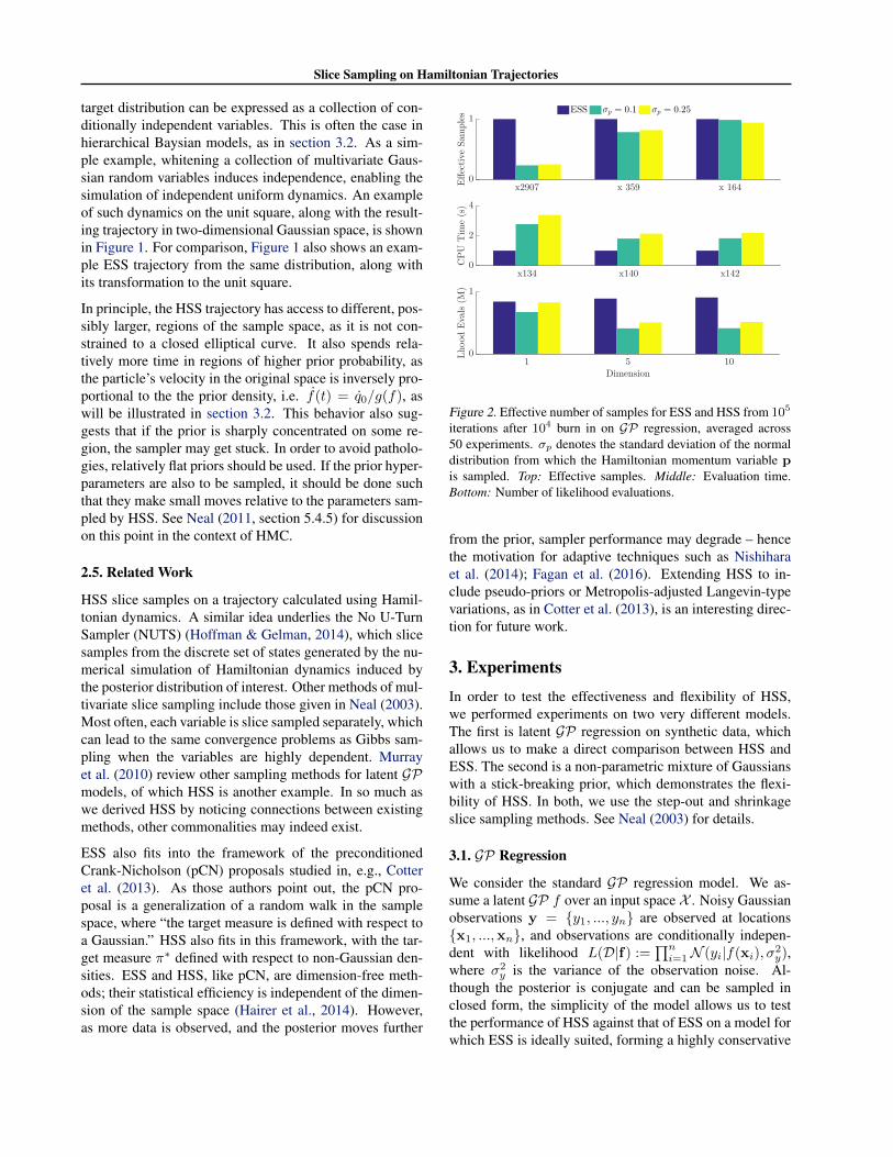
Figure 3. Top: Trajectories on the simplex used by HSS (left) and HMC (right) to generate two samples of stick weights Vk from a toyversion of the model described in section 3.2, withK = 3. The contours of the posterior are shown, and order of the samples is indicatedby the number on the sample point. Bottom: The trajectories for V1 and V2 corresponding to the first sample. (V3 is fixed at 1.) Thewidth of the trajectory (top) and shading (bottom) in the HSS plots is proportional to the inverse of the particle’s velocity, and representsthe probability mass placed by the slice sampler, which samples uniformly on the slice in t, on the corresponding part of sample space.

For comparison, we also used HMC to update the clusterparameters. HMC uses the gradient of the posterior andso should be expected to generate good posterior samples,if properly tuned. Figure 3 compares the behavior of HSSand HMC trajectories on the simplex in a toy example. Toquatitatively compare HSS with HMC in a real data setting,we fit a simple one-dimensional Gaussian mixture modelwith a Gaussian prior on the cluster means, and a Gammaprior on the cluster precisions using the galaxy dataset, withn = 82 observations, that was also used in Favaro & Teh(2013); Lomeli et al. (2015).

In order to sample from the posterior distribution, we ranexperiments with HSS or HMC embedded in the hybridGibbs sampler, fixing the hyperparameters at α = 0.3 andθ = 1. HSS was relatively easy to tune to achieve goodconvergence and mixing, with slice sampling parametersw = 1, and m = ∞. The different groups of latent vari-ables in the model had very different scaling, and we foundthat σp = 0.1 and setting the mass equal to mv = 1 forthe {Vk}, and mn = mγ = 10 for the cluster means andprecisions worked well. So as to compare the computa-tion time between similar effective sample sizes (see sec-tion 3.3 below), we set the HMC parameters to achieve anacceptance ratio near 1, which required simulation steps of

size ε ∈ [5× 10−5, 15× 10−5], sampled uniformly fromthat range for each sampling iteration. We ran HMC withL ∈ {60, 150} steps for comparison. The results, displayedin Figure 4, show the relative efficiency of HSS; it achievesmore effective samples per unit of computation time.

We note that HMC’s performance improves, as measuredby effective sample size, with larger simulation step sizes.However, larger simulation steps result in a non-trivial pro-portion of rejected HMC proposals, making impossible di-rect comparison with HSS due to the issue discussed in thefollowing section. We also observed that the performanceof HSS degraded with increasing sample size, because theposterior looks less like the prior, and the discussion in sec-tion 2.5 suggests. This behavior indicates that the use of apseudo-prior would be beneficial in many situations.

3.3. Effective Sample Size in BNP Mixture Models

It is worth noting that the effective sample size (in log-jointprobability) achieved by HSS in our experiments for thePY model are an order of magnitude lower than those re-ported by Favaro & Teh (2013); Lomeli et al. (2015), whocalculated effective samples ofK∗, the number of occupiedclusters. While conducting preliminary tuning runs of the

Slice Sampling on Hamiltonian Trajectories

HSS HMC,L = 60

HMC,L = 150

Eff.Sam

ples(JLL)per

RunTim

e(m

in)

0

0.5

1

1.5

Figure 4. Effective number of samples per minute of run time forHSS and HMC from 105 samples taken at intervals of 20 inter-ations, after 104 burn in iterations on the PY model, averagedacross 10 experiments. L is the number of simulation steps usedby HMC at each sampling iteration.

HMC sampler, we observed something odd: if the HMCsimulations were not properly tuned, and thus almost everyproposed HMC move was rejected, the resulting effectivesample size in K∗ was of the order of those previously re-ported. Further experiments in which we artificially limitedHMC and HSS to take small steps produced the same ef-fect: samplng efficiency, as measured either by K∗ or log-joint probability, benefits from small (or no) changes in thecluster parameters. It seems that when the parameter clus-ters do a suboptimal job of explaining the data, the clusterassignment step destroys many of the clusters and createsnew ones, sampling new parameters for each. This oftenhappens when the parameter update step produces small orno changes to the cluster parameters. The result is stepsin sample space that appear nearly independent, and corre-spondingly a large effective sample size, despite the unde-sireably small moves of the parameter updates. This under-scores the importance of better measures of sample quality,especially for complicated latent variable models.

4. DiscussionRecognizing a link between two popular sampling meth-ods, HMC and slice sampling, we have proposed Hamil-tonian slice sampling, a general slice sampling algorithmbased on analytic Hamiltonian trajectories. We describedconditions under which analytic (possibly transformed)Hamiltonian trajectories can be guaranteed, and we demon-strated the simplicity and usefulness of HSS on two verydifferent models: Gaussian process regression and mix-ture modeling with a stick-breaking prior. The former GPcase is where ESS is particularly expected to perform, and

in reasonable dimensionality we showed HSS performedcompetitively. The latterPY case is where we expect HMCto be more competitive (and where ESS does not apply).Here we found that HSS had a similar effective sample sizebut outperformed even carefully tuned HMC in terms ofcomputational burden. As speed, scaling, and generalityare always critical with MCMC methods, these results sug-gest HSS is a viable method for future study and applica-tion.

AcknowledgementsWe thank Francois Fagan and Jalaj Bhandari for useful dis-cussions, and for pointing out an error in an earlier draft;and anonymous referees for helpful suggestions. JPC issupported by funding from the Sloan Foundation and theMcKnight Foundation.

ReferencesBetancourt, M. J., Byrne, Simon, Livingstone, Samuel, and

Girolami, Mark. The Geometric Foundations of Hamil-tonian Monte Carlo. Bernoulli, (to appear), 2016.

Cotter, S. L., Roberts, G. O., Stuart, A. M., and White, D.MCMC Methods for Functions: Modifying Old Algo-rithms to Make Them Faster. Statist. Sci., 28(3):424–446, 2013.

Fagan, Francois, Bhandari, Jalaj, and Cunningham, John P.Elliptical Slice Sampling with Expectation Propagation.In Proceedings of the 32nd Conference on Uncertaintyin Artificial Intelligence, volume (To appear), 2016.

Favaro, Stefano and Teh, Yee Whye. MCMC for Normal-ized Random Measure Mixture Models. Statist. Sci., 28(3):335–359, 2013.

Girolami, Mark and Calderhead, Ben. Riemann manifoldLangevin and Hamiltonian Monte Carlo methods. Jour-nal of the Royal Statistical Society: Series B (StatisticalMethodology), 73(2):123–214, 2011. ISSN 1467-9868.

Hairer, Martin, Stuart, Andrew M., and Vollmer, Sebas-tian J. Spectral gaps for a Metropolis–Hastings algo-rithm in infinite dimensions. Ann. Appl. Probab., 24(6):2455–2490, 2014.

Hoffman, Matthew D. and Gelman, Andrew. The No-U-Turn Sampler: Adaptively Setting Path Lengths inHamiltonian Monte Carlo. Journal of Machine Learn-ing Research, 15:1593–1623, 2014.

Ishwaran, Hemant and James, Lancelot F. Gibbs SamplingMethods for Stick-Breaking Priors. Journal of the Amer-ican Statistical Association, 96(453):161–173, 2001.

Slice Sampling on Hamiltonian Trajectories

Kalli, Maria, Griffin, Jim E., and Walker, Stephen G. Slicesampling mixture models. Statistics and Computing, 21(1):93–105, 2011.

Lomeli, Maria, Favaro, Stefano, and Teh, Yee Whye. A hy-brid sampler for Poisson-Kingman mixture models. InCortes, C., Lawrence, N.D., Lee, D.D., Sugiyama, M.,Garnett, R., and Garnett, R. (eds.), Advances in Neu-ral Information Processing Systems 28, pp. 2152–2160.Curran Associates, Inc., 2015.

Murray, Iain, Adams, Ryan P., and MacKay, David J.C. El-liptical slice sampling. JMLR: W&CP, 9:541–548, 2010.

Neal, Radford M. Slice sampling. Ann. Statist., 31(3):705–767, 2003.

Neal, Radford M. Handbook of Markov Chain MonteCarlo, chapter 5: MCMC using Hamiltonian dynamics,pp. 113–162. Chapman and Hall/CRC, 2011.

Nishihara, Robert, Murray, Iain, and Adams, Ryan P. Par-allel MCMC with Generalized Elliptical Slice Sampling.Journal of Machine Learning Research, 15:2087–2112,2014.

Pakman, Ari and Paninski, Liam. Auxiliary-variable Ex-act Hamiltonian Monte Carlo Samplers for Binary Dis-tributions. In Burges, C.J.C., Bottou, L., Welling, M.,Ghahramani, Z., and Weinberger, K.Q. (eds.), Advancesin Neural Information Processing Systems 26, pp. 2490–2498. Curran Associates, Inc., 2013.

Pakman, Ari and Paninski, Liam. Exact HamiltonianMonte Carlo for Truncated Multivariate Gaussians.Journal of Computational and Graphical Statistics, 23(2):518–542, 2014.

Plummer, Martyn, Best, Nicky, Cowles, Kate, and Vines,Karen. CODA: Convergence Diagnosis and OutputAnalysis for MCMC. R News, 6(1):7–11, 2006.

Strathmann, Heiko, Sejdinovic, Dino, Livingstone,Samuel, Szabo, Zoltan, and Gretton, Arthur. Gradient-free Hamiltonian Monte Carlo with Efficient Kernel Ex-ponential Families. In Cortes, C., Lawrence, N.D., Lee,D.D., Sugiyama, M., and Garnett, R. (eds.), Advancesin Neural Information Processing Systems 28, pp. 955–963. Curran Associates, Inc., 2015.

Wang, Ziyu, Mohamed, Shakir, and de Freitas, Nando.Adaptive Hamiltonian and Riemann Manifold MonteCarlo. In Dasgupta, Sanjoy and Mcallester, David (eds.),Proceedings of the 30th International Conference onMachine Learning (ICML-13), volume 28, pp. 1462–1470. JMLR Workshop and Conference Proceedings,2013.