Embed Size (px)
Citation preview

arX
iv:a
stro
-ph/
0412
126v
1 6
Dec
200
4
Transmission of light in deep sea water at the
site of the Antares neutrino telescope
The ANTARES Collaboration
J.A. Aguilar a, A. Albert b, P. Amram c, M. Anghinolfi d, G. Anton e,S. Anvar f , F.E. Ardellier-Desages f , E. Aslanides g, J-J. Aubert g,
R. Azoulay f , D. Bailey h, S. Basa g, M. Battaglieri d, Y. Becherini i,R. Bellotti j, J. Beltramelli f , V. Bertin g, M. Billault g, R. Blaes b, F. Blanc k,
R.W. Bland f 1 , N. de Botton f , J. Boulesteix c, M.C. Bouwhuis ℓ,C.B. Brooks h, S.M. Bradbury m, R. Bruijn ℓ, J. Brunner g, F. Bugeon f ,G.F. Burgio n, F. Cafagna j, A. Calzas g, L. Caponetto n, E. Carmona a,J. Carr g, S.L. Cartwright o, S. Cecchini i,p, P. Charvis q, M. Circella j,C. Colnard ℓ, C. Compere r, J. Croquette r, S. Cooper h, P. Coyle g,
S. Cuneo d, G. Damy r, R. van Dantzig ℓ, A. Deschamps q, C. De Marzo j,J-J. Destelle g, R. De Vita d, B. Dinkelspiler g, G. Dispau f , J-F. Drougou s,
F. Druillole f , J. Engelen ℓ, S. Favard g, F. Feinstein g 2 , S. Ferry t, D. Festy r,J. Fopma h, J-L. Fuda k, J-M. Gallone t, G. Giacomelli i, N. Girard b,
P. Goret f , J-F. Gournay f , G. Hallewell g, B. Hartmann e, A. Heijboer ℓ,Y. Hello q, J.J. Hernandez-Rey a, G. Herrouin s, J. Hoßl e, C. Hoffmann t,J. R. Hubbard f , M. Jaquet g, M. de Jong ℓ, F. Jouvenot f , A. Kappes e,
T. Karg e, S. Karkar g, M. Karolak f , U. Katz e, P. Keller g, P. Kooijman ℓ,E.V. Korolkova o, A. Kouchner u,f , W. Kretschmer e, V.A. Kudryavtsev o,
H. Lafoux f , P. Lagier g, P. Lamare f , J-C. Languillat f , L. Laubier k,T. Legou g, Y. Le Guen r, H. Le Provost f , A. Le Van Suu g, L. Lo Nigro n,
D. Lo Presti n, S. Loucatos f , F. Louis f , V. Lyashuk v, P. Magnier f ,M. Marcelin c, A. Margiotta i, C. Maron q, A. Massol s, F. Mazeas r,B. Mazeau f , A. Mazure c, J.E. McMillan o, J-L. Michel s, C. Millot k,
A. Milovanovic m, F. Montanet g, T. Montaruli j, J-P. Morel r, L. Moscoso f ,E. Nezri g, V. Niess g, G.J. Nooren ℓ, P. Ogden m, C. Olivetto t,
N. Palanque-Delabrouille f 3 , P. Payre g, C. Petta n, J-P. Pineau t,J. Poinsignon f , V. Popa i,w, R. Potheau g, T. Pradier t, C. Racca t,
N. Randazzo n, D. Real a, B.A.P. van Rens ℓ, F. Rethore g, M. Ripani d,V. Roca-Blay a, A. Romeyer f , J-F. Rollin r, M. Romita j, H.J. Rose m,
1 Now at: Dpt. of Physics & Astronomy, San Francisco State University,1600 Holloway Avenue, San Francisco, CA94132, USA2 Now at: Groupe d’Astroparticules de Montpellier, UMR 5139-UM2/IN2P3-CNRS, Universite Montpellier II, Place Eugene Bataillon - CC85, 34095 MontpellierCedex 5, France3 Corresponding author.E-mail address: [email protected]
Preprint to be submitted to Astroparticle Physics 26 November 2011

A. Rostovtsev v, M. Ruppi j, G.V. Russo n, Y. Sacquin f , S. Saouter f ,J-P. Schuller f , W. Schuster h, I. Sokalski j, O. Suvorova b 4 , N.J.C. Spooner o,
M. Spurio i, T. Stolarczyk f , D. Stubert b, M. Taiuti d, L.F. Thompson o,S. Tilav h, A. Usik v, P. Valdy s, B. Vallage f , G. Vaudaine a, P. Vernin f ,
J. Virieux q, E. Vladimirsky v, G. de Vries ℓ, P. de Witt Huberts ℓ,E. de Wolf ℓ, D. Zaborov v, H. Zaccone f , V. Zakharov v, S. Zavatarelli d,
J. de D. Zornoza a, J. Zuniga a
4 Now at: Academy of Science, Institute for Nuclear Research, 60th OctoberAnniversary Prospect 7a, RU-117312, Moscow, Russia
2

aIFIC – Instituto de Fısica Corpuscular, Edificios Investigacion de Paterna, CSIC– Universitat de Valencia, Apdo. de Correos 22085, 46071 Valencia, Spain
bGRPHE – Groupe de Recherches en Physique des Hautes Energies, Universite deHaute Alsace, 61 Rue Albert Camus, 68093 Mulhouse Cedex, France
cLAM – Laboratoire d’Astrophysique de Marseille, CNRS/INSU - Universite deProvence Aix-Marseille I, Traverse du Siphon – Les Trois Lucs, BP 8, 13012
Marseille Cedex 12, FrancedDipartimento di Fisica dell’Universita e Sezione INFN, Via Dodecaneso 33,
16146 Genova, ItalyeUniversity of Erlangen,Friedrich-Alexander Universitat Erlangen-Nurnberg,
Physikalisches Institut,Erwin-Rommel-Str. 1, 91058 Erlangen, GermanyfDSM/DAPNIA – Direction des Sciences de la Matiere, Departement
d’Astrophysique de Physique des Particules de Physique Nucleaire et del’Instrumentation Associee, CEA/Saclay, 91191 Gif-sur-Yvette Cedex, France
gCPPM – Centre de Physique des Particules de Marseille, CNRS/IN2P3Universite de la Mediterranee Aix-Marseille II, 163 Avenue de Luminy, Case 907,
13288 Marseille Cedex 9, FrancehUniversity of Oxford, Department of Physics, Nuclear and Astrophysics
Laboratory, Keble Road, Oxford OX1 3RH, United KingdomiDipartimento di Fisica dell’Universita e Sezione INFN, Viale Berti Pichat 6/2,
40127 Bologna, ItalyjDipartimento Interateneo di Fisica e Sezione INFN, Via E. Orabona 4, 70126
Bari, ItalykCOM – Centre d’Oceanologie de Marseille, CNRS/INSU Universite de la
Mediterranee Aix-Marseille II, Station Marine d’Endoume-Luminy, Rue de laBatterie des Lions, 13007 Marseille, France
ℓNIKHEF, Kruislaan 409, 1009 SJ Amsterdam, The NetherlandsmUniversity of Leeds, Department of Physics and Astronomy, Leeds LS2 9JT,
United KingdomnDipartimento di Fisica ed Astronomia dell’Universita e Sezione INFN, Viale
Andrea Doria 6, 95125 Catania, ItalyoUniversity of Sheffield, Department of Physics and Astronomy, Hicks Building,
Hounsfield Road, Sheffield S3 7RH, United KingdompIASF/CNR, 40129 Bologna, Italy
qUMR GoScience Azur, Observatoire Ocanologique de Villefranche, BP48, Portde la Darse, 06235 Villefranche-sur-Mer Cedex, France
rIFREMER – Centre de Brest, BP 70, 29280 Plouzane, FrancesIFREMER – Centre de Toulon/La Seyne Sur Mer, Port Bregaillon, Chemin
Jean-Marie Fritz, 83500 La Seyne Sur Mer, FrancetIReS – Institut de Recherches Subatomiques (CNRS/IN2P3), Universite Louis
Pasteur, BP 28, 67037 Strasbourg Cedex 2, France
3

uUniversite Paris VII, Laboratoire APC, UFR de Physique, 2 Place Jussieu,75005 Paris, France
vITEP – Institute for Theoretical and Experimental Physics,B. Cheremushkinskaya 25, 117259 Moscow, Russia
wISS – Institute for Space Siences, 77125 Bucharest – Magurele, Romania
Abstract
The ANTARES neutrino telescope is a large photomultiplier array designed to de-tect neutrino-induced upward-going muons by their Cherenkov radiation. Under-standing the absorption and scattering of light in the deep Mediterranean is fun-damental to optimising the design and performance of the detector. This paperpresents measurements of blue and UV light transmission at the ANTARES sitetaken between 1997 and 2000. The derived values for the scattering length and theangular distribution of particulate scattering were found to be highly correlated, andresults are therefore presented in terms of an absorption length λabs and an effectivescattering length λeff
sct. The values for blue (UV) light are found to be λabs ≃ 60(26)m, λeff
sct ≃ 265(122) m, with significant (∼15%) time variability. Finally, the re-sults of ANTARES simulations showing the effect of these water properties on theanticipated performance of the detector are presented.
Key words: Neutrino telescope; Undersea Cherenkov detectors; Sea waterproperties: absorption and transmission of light.PACS: 07.89.+b, 29.40.Ka, 42.25.Bs, 42.68.Xy, 92.10.Bf, 92.10.Pt, 95.55.Vj
4

1 Introduction
The Antares 5 undersea neutrino telescope [1] will use an array of photomul-tiplier tubes (PMT) in the deep Mediterranean Sea to detect the Cherenkovlight emitted by muons resulting from the interaction of high energy neutrinoswith matter. The muon track is reconstructed from the arrival time of detectedphotons. The performance of the detector is therefore critically dependent onthe optical properties of sea water, in particular on the velocity of light and onthe absorption and scattering cross-sections. All these parameters vary withthe photon wavelength. The relevant spectrum spans from ultraviolet to green(see figure 1); the Cherenkov light spectrum varies like 1/λ2, the photomul-tiplier tube quantum efficiency becomes too low to probe wavelengths longerthan 600 nm, while the glass pressure sphere that surrounds the phototubeabsorbs the light at wavelengths shorter than 320 nm. Seasonal variationsin sedimentation in the sea water [2] might induce variations in the opticalparameters.
Several measurements of sea water attenuation have been performed in thepast. The Dumand collaboration reported an attenuation length varying withthe light wavelength and reaching a maximum value of 60 m, with 50% ac-curacy, for a wavelength of 500 nm [4]. The Nestor collaboration measured asimilar behaviour. The maximum attenuation length was found at 490 nm andwas estimated to be 55 ± 10 m [5]. The Baikal experiment found a maximumabsorption length of about 20 m for a wavelength of 490 nm [6]. Measurementsperformed in pure water show that the maximum of the attenuation length isat lower values of the wavelength in this medium (∼ 400 nm) [7,8]. The max-imum value was measured around 90 m with 40% accuracy. More recently,measurements of the absorption spectrum in pure water have been reported,with maximum absorption lengths of 160 ± 15 m at 420 nm [9] and of 225 ±30 m at 417 nm [10].
In order to reach an optimal knowledge of the light propagation propertiesat the detector site all relevant parameters concerning photon absorption andscattering should be measured. These parameters, described in section 3, willbe directly measured and continuously monitored by the Antares exper-iment using an instrumentation line. Until now, the adopted approach hasbeen to measure these parameters with in situ autonomous devices, and thesemeasurements are the subject of this paper. We present time-of-flight distribu-tions of photons emitted from a pulsed isotropic light source and detected bya PMT at different distances from the source and for two wavelengths (blueand UV, as indicated in figure 1). Knowledge of the time-of-flight distribu-tion is essential in order to reconstruct muon tracks. While this approach is
5 http://antares.in2p3.fr
5
0
0.05
0.1
0.15
0.2
0.25
300 350 400 450 500 550 600λ (nm)
Det
ecti
on
eff
icie
ncy
UV B
Fig. 1. Detection efficiency as a function of wavelength. The solid curve shows thePMT quantum efficiency and the absorption by the glass of the PMT, the opticalgel and the protective glass sphere housing the PMT [25]. The dashed and dottedcurves are calculated with a path length in water of 5 m and 30 m respectively,assuming a characteristic wavelength dependence of the water absorption lengthas given in [3]. The effect of scattering is not included. The bands labelled “B”and “UV” indicate the wavelengths at which measurements were undertaken at theAntares site.
not sufficient to fully determine the differential cross section of the photonscattering process, the absorption length can be measured unambiguously. Aparameterisation which reproduces the main features of the scattering processcan be obtained, sufficient for the needs of the tracking algorithms and of thedetector simulation.
2 Experimental setup and measurement procedure
The site chosen for the deployment of the detector is southeast of Toulon(42◦50′N 6◦10′E), 40 km from shore at a depth of 2475 m. During several seacampaigns from 1997 to 2000 we have improved the experimental setup de-voted to the study of the light transmission properties, and refined the analysisof the data. We focus, in this section, on the final experimental configuration.
6

2.1 The mooring line
The measuring system is mounted on an autonomous mooring line anchoredby a sinker. The line remains vertical through the flotation provided by syn-tactic buoys. After deployment, an acoustic modem 6 is used to control themeasurement from the surface ship which stays in the vicinity of the zonewhere the line was sunk. A sketch of the mooring line including informationon approximate heights from the sea floor is displayed in figure 2.
The measuring system consists of 17′′ pressure resistant glass spheres mountedon two triangular aluminum frames. A set of three mechanical cables attachedto the vertices of the two frames defines their separation distance. The bot-tom frame supports a light source sphere which contains a set of LEDs withtheir pulsers. The top frame supports a detector sphere facing the light sourcesphere, and a service sphere (cf. figure 5). The detector sphere houses a pho-tomultiplier tube, the DC-DC converter which supplies the high voltage and apulse height discriminator providing a timing signal for each detected photon.The service sphere contains a TDC, a microprocessor which controls the mea-surement and records the data, and a set of lithium batteries which power thesystem. An acoustic modem remote unit is located on top of the measuringsystem.
2.2 The light source sphere
In order to obtain an isotropic light source for two wavelengths, 6 pairs ofLEDs were mounted on the centres of the faces of a cubic frame 3 cm on aside which also supports the LED pulser boards. Each pair, which includesa blue and a UV LED, is covered with a single 1 cm diameter diffusing capconsisting of glass micro-spheres embedded in epoxy. The cube is installed atthe centre of a 17′′ glass sphere whose external surface has been sand blasted toprovide extra diffusion and to remove surface ripples or roughness which candestroy the homogeneity of the emitted light flux. The blue or UV emissioncolour is chosen for each new acquisition by the operator; all 6 LEDs of theselected colour are then flashed simultaneously.
The spectrum of the light emitted by the LEDs was measured using a spectro-photometre (see figure 3). The peak wavelength and the spectrum FWHM inpulsed mode operation are (375 nm, 10 nm) and (473 nm, 29 nm) respectivelyfor the UV and blue LED. The time distribution of photons emitted by thelight source sphere was measured in a dark room for both colours using thecomplete system (see figure 4) and has a FWHM of about 9 ns, with a tail
6 ATM 845/851 from Datasonic (now Benthos), www.benthos.com
7

source sphere
detector sphere
service sphere
buoys
buoys
buoys
acoustic modem
buoys
ARGOS buoy
ANTARESLight transmission line
parafil cables
anchor
acoustic releases
10 m
15 to 44 m
50 m
10 m
50 m
Fig. 2. Sketch of the mooring line used for the measurements of the water transmis-sion properties. The figure is not to scale.
towards longer times. The isotropy of the source was checked to be within±12% by measuring the light flux for different orientations of the source spherewith respect to the detector sphere.
8

0
250
500
750
1000
1250
1500
1750
2000
360 380 400 420 440 460
Pulsed mode
λpeak = 375 nmFWHM = 10 nm
UV LED
wavelength (nm)
(a) UV LED
0
200
400
600
800
1000
1200
1400
1600
420 440 460 480 500 520
Blue LED
Pulsed mode
λpeak = 473 nmFWHM = 29nm
wavelength (nm)
(b) Blue LED
Fig. 3. Spectral emission of the blue and UV LEDs (smoothed curves, intensity inarbitrary units). The light and dark areas correspond to the two extreme valuesof the range of source intensities used for the measurements, with no significantdifference in the spectra.
2.3 The detector sphere
A small 1′′ diameter photomultiplier tube 7 glued on the internal surface ofa 17′′ sphere detects photons emitted by the light source. The size of thePMT was chosen in order to limit the counting rate from deep sea opticalbackground. The PMT was then selected for its speed and low transit timespread. Except for the PMT window, the internal surface of the detector sphereis blackened in order to absorb photons outside the PMT detection solid angle.
2.4 The service sphere
The service sphere provides a 6 kHz trigger signal which is fed to the LEDpulsers and through a delay to a TDC (cf. figure 5). The TDC is started bythe delayed trigger signal and stopped by the first PMT signal above the dis-criminator threshold. The clock of the TDC is defined by a 40 MHz quartzoscillator with each 25 ns period subdivided into 32 approximately equal chan-nels giving an average δt = 0.78 ns time bin. The TDC range can be adjustedby defining its active window; during most of the measurements it was set to
7 Photomultiplier tube 9125 SA from EMI, now ETL,www.electron-tubes.co.uk/splash.html
9

10-5
10-4
10-3
10-2
10-1
-20 0 20 40 60 80 100 120 140 160 180
Blue source
FWHM = 9.5 ns
time (ns)
10-5
10-4
10-3
10-2
10-1
-20 0 20 40 60 80 100 120 140 160 180
UV source
FWHM = 9.2 ns
time (ns)
Fig. 4. Normalised distributions of photon arrival times measured in air with highstatistics for the complete source sphere and with the full setup. Collimators arelocated between the source and the detector spheres.
MBXprocessor
TDC
HV converter
Discriminator1’’ PMT
Delay
Start
Stop
LED trigger
InterfaceBoard
8 bit bus
6 LEDsin a sand blasted sphere
(isotropic illumination pattern)PMT HV monitoring and control
Trigger
Fig. 5. Sketch of the acquisition system.
1100 channels in order to accommodate the time distributions for all of thesource-detector distances investigated.
The TDC linearity was studied in a dark room by recording a white noisespectrum with high statistics; in the absence of LED flashes, the PMT stopsignals were provided by the background created by a controlled light leak.A typical white noise spectrum is displayed in figure 6, showing the non-linearities associated with the 32 channel subdivision pattern. A negative slopein the data is expected, due to the fact that the TDC is single-hit (i.e. stoppedby the first PMT signal) and thus cannot record the arrival time of furtherphotons; earlier hits are favoured over later ones. The probability pi that a hit
10

is recorded in bin i given a flat distribution of arrival time is (to first order)pi = R δt × (1 − R δt)(i−1) ≃ R δt × [1 − (i − 1) R δt] where R is the rate ofbackground noise.
bin number
cou
nts
0
2000
4000
6000
8000
10000
12000
0 200 400 600 800 1000
bin number
ZOOM
3000
3200
3400
3600
3800
4000
400 420 440 460 480 500 520 540 560 580 600
Fig. 6. White noise time distribution for TDC calibration. In the enlargement, thenon-linearities of the TDC are seen. Given their high noise level, the first (notshown) and last few bins were not used for the recording of physics data.
2.5 Experimental procedure
The cable lengths are set on board for the desired source-detector distance(ranging from 15 to 44 m). Two cable lengths are typically used for eachchoice of LED voltage.
After the line has reached the sea bed, the acoustic link is established from thesurface ship. The light intensity is adjusted via the voltage on the LED pulsersto give a detection efficiency of about 1 detected photon per 100 triggers for theshortest source-detector distance. This ensures that the PMT is working closeto the single photoelectron regime. The detection efficiency can artificiallyincrease because of intermittent luminescence bursts. The same intensity isthen used for the longer distance. The discriminator threshold is set at a pulseheight value of 0.3 times the amplitude of the single-photoelectron peak, in thevalley between the peak and the noise. For a given source-detector distance,several data sets corresponding typically to 5×10⁶ triggers each were collectedfor each of the two light colours. The overall time needed to perform the
11

measurements at one source-detector distance including the drop and recoveryof the line is approximately 4 hours.
The various measurements of the water optical properties at the Antares
site from 1997 to 2000 are summarised in table 1, in chronological order.
SourcedSD Time of
Comment(in m) year
Blue 6 – 27 Dec. 1997 Different setup (cf. text)
Blue 24, 44 July 1998 2 source intensities
Blue 24, 44 March 1999 standard
UV 15, 24 July 1999 standard
UV 24, 44 Sept. 1999 standard
Blue, UV 24, 44 June 2000 standard
Blue, UV 24 June 2000 400 m above the sea bed
Table 1Data recorded for the study of the water light transmission properties. The stan-dard configuration is: measurement of the arrival time distribution of photons froma pulsed isotropic source, one source intensity (same for the two source-detectordistances dSD), source sphere located 100 m above the sea bed (figure 2).
The July 1998 data taken with two source intensities I1 and I2 are used tostudy the systematics coming from the shape of the source time distribution,which exhibits a slight dependence on the LED pulser voltage (16.5 V inthe first case, 18 V in the second). The data recorded 400 m above the seabed (June 2000) were compared to the other data recorded at 100 m abovesea bed to check the water transparency dependence over this depth range,corresponding to the instrumented range of the Antares detector.
As illustrated in figure 7, all the time distributions recorded (1998 to 2000) ex-hibit a small tail of delayed photons. This corresponds to a small contributiondue to scattering between the source and the detector. Figure 8 illustrates,for June 2000 standard blue and UV data, the shape of the photon arrivaltime distribution in air (no scattering), and in water with a source-detectordistance dSD = 24 m or dSD = 44 m. Clearly, the width of the main peak comesmostly from time resolution of the setup. The FWHM of spectra recorded fora source-detector distance of 24 m is about 10 ns, to be compared with theintrinsic FWHM of 9 ns of the light source. As expected, the scattering tailincreases with a larger separation between the source and the detector. Scat-tering is also seen to be more significant in UV than in blue: slightly largerincrease of the width of the peak region and higher scattering tail, in particularat a distance of 44 m.
12

0
0.01
0.02
0.03
0.04
0.05
0.06
0.07
0 50 100 150 200 250 300
time delay (ns)
UV
24m data
44m data
Fig. 7. Time distributions in UV light for the two source-detector distances (24 and44 m) of the first June 2000 immersion. Y-axis is proportional to the number of pho-tons collected. The 24 m distribution is normalised to unity. The 44 m distributionis normalised with respect to the one at 24 m, in addition to a (44/24)2 factor, sothe difference between the two peaks is entirely due to the exponential attenuationfactor.
10-3
10-2
10-1
1
-20 0 20 40 60 80 100 120 140
collimated air data24 m data44 m data
time delay (in ns)
BLUE
10-3
10-2
10-1
1
-20 0 20 40 60 80 100 120 140
collimated air data24 m data44 m data
time delay (in ns)
UV
Fig. 8. Photon arrival times for a collimated air time distribution and for two distri-butions taken in situ, with source-detector distances of 24 m and 44 m. All distribu-tions are normalised to unity at the peak. Top panel: June 2000 blue data. Bottompanel: June 2000 UV data. The origin of the time delay axis is set to 0 for directphotons.
13
The setup deployed for the first immersion (December 1997) was differentfrom the one described above. An 8′′ photomultiplier tube is located at avariable distance (6 to 27 m) from a collimated continuous blue LED source(λ = 466 nm). Only the integrated intensity was recorded. The analysis of thedata from this immersion is described in section 4.3. All subsequent immersionswere done with the setup described in sections 2.1 to 2.4.
3 Simulation of the experiment
The photon propagation (hence the time distribution of photons at a distanceR from the source) is governed by the following inherent optical parameters:group velocity of light in the medium vg, absorption length λabs, and volume
scattering function β(θ) = β(θ)/λsct with units m−1 · sr−1 (where β(θ) is thenormalised scattering angle distribution and λsct the scattering length). Thescattering function is roughly described by the scattering length λsct and theaverage cosine of the scattering angle distribution (or asymmetry parameter)〈cos θ〉 = 2π
∫β(θ) cos θ d(cos θ), under the assumption of a specific shape of
the scattering angle distribution.
3.1 Physics of propagation of light in sea water
For an isotropic source of photons with intensity I0, the intensity I detectedat a distance R from the source by a PMT with an active area A is
I = I0A
4πR2e−R/λeff
att , (1)
where λeffatt is the effective attenuation length, extracted from the total number
of photons (i.e. from the integrated time distributions) recorded for two source-detector distances.
An approximate degeneracy reduces the number of parameters needed to char-acterise the time distribution of photons at a distance R from the source. Inparticular, strong correlations can be expected if trying to extract 〈cos θ〉 andλsct separately, while λeff
sct, defined as
λeffsct ≡
λsct
1 − 〈cos θ〉, (2)
14

describes the main part of the scattering. 8
We describe the scattering angle distribution following the approach of Moreland Loisel [12]: the scattering angle distribution is expressed as the weightedsum of molecular and particulate scattering. The molecular scattering is de-scribed by the Einstein-Smoluchowski formula for pure water,
βm(cos θ) = 0.06225 (1 + 0.835 cos2 θ) , (3)
which is reminiscent of the form
βRay(cos θ) =3
16π(1 + cos2 θ) , (4)
commonly called Rayleigh scattering. The 0.835 factor (rather than 1) is at-tributable to the anisotropy of the water molecules. The particulate scatteringis described by the Mobley et al. [13] tabulated distribution βp(cos θ), obtainedby averaging the similar particulate angle distributions measured by Petzoldin very different seas [14], at a wavelength of 514 nm.
The total normalised scattering angle distribution is of the form:
β(cos θ) = ηβm(cos θ) + (1 − η)βp(cos θ) , (5)
with η the ratio of molecular to total scattering. The average cosine of thetotal scattering angular distribution is
〈cos θ〉 = (1 − η) × 〈cos θ〉p = (1 − η) × 0.924 , (6)
8 As a general property of multiple scattering [11], the average cosine of the lightfield produced by a thin narrow parallel beam after n scattering events 〈cos θ〉n isrelated to the average cosine for single scattering 〈cos θ〉 by the relation 〈cos θ〉n =〈cos θ〉n . The average number of scattering events undergone by a photon reaching adistance R from the source is n = L(R)/λsct where L(R) is the average path lengthof these photons. If scattering is dominantly at small angle, as in natural waters, wehave n ≃ R/λsct. Therefore the average cosine of the light field at distance R fromthe source is: 〈cos θ〉R ≃ 〈cos θ〉R/λsct . All combinations of λsct and 〈cos θ〉 that givethe same effective scattering length
λeffsct =
λsct
− ln〈cos θ〉
yield the same 〈cos θ〉R. In the case where 〈cos θ〉 ≃ 1, the above relation becomesequation 2.
15

since the average cosine of Petzold’s distribution is 0.924. In natural waters,η is typically less than 0.2 [12], so 〈cos θ〉 is large and the use of equation 2 isjustified.
3.2 The Monte Carlo simulation
A detailed Monte Carlo simulation, which includes the geometry of the ex-perimental setup and the optical properties of the medium, has been used toanalyze the experimental time distributions and extract the light transmissionparameters at the Antares site. The parameters of the Monte Carlo are theabsorption length λabs, the scattering length λsct, the fraction η of molecularscattering, the source-detector distances di, the origin of time for each distri-bution (or the time ti at which direct photons reach the detector located at adistance di from the source) and the collection efficiency for each distribution.
For each photon, the distance x it will travel before being absorbed is selectedrandomly from the probability distribution proportional to exp(−x/λabs). Thephoton’s distance to its first scattering is similarly selected according to exp(−x/λsct).If the absorption distance is shorter, the photon is propagated to its point ofabsorption and stopped. Otherwise, the type of scattering (molecular or par-ticulate) is selected according to their respective probabilities η and 1−η; thephoton is propagated to its point of scattering where a new photon directionis sampled from the appropriate angular distribution and a new scatteringdistance is drawn. This is repeated until the total length of the photon pathreaches its absorption distance. Time distribution histograms are filled when-ever the photon reaches a radial distance from the source corresponding toone of the possible source-detector separations. Weights are applied to takeinto account the dependence of the PMT detection efficiency on the angleof incidence of the photon on the photocathode [15] or to study a possibleanisotropy of the source emission. Each Monte Carlo distribution results fromthe propagation of one million photons.
The time distribution of the emitted light pulse is taken from the one measuredin air for direct photons (see figure 4), its angular distribution is taken asisotropic, and its spectrum as monochromatic (see actual spectral width infigure 3) at its central wavelength.
The obtained Monte Carlo photon spectrum corresponds to a light source witha vanishingly small intensity, dominated by single photon events. For realisticintensity conditions, since the TDC is working in the single hit mode, oneneeds to correct the spectrum for multi-photon events where the first one onlyis detected. This correction depends on the average rate of detection per lightpulse trigger, and is calculated assuming Poisson statistics. The background
16

is removed from the data spectra (see section 4.1 on the data processing) soMonte Carlo spectra are generated with no noise.
4 Data analysis
4.1 Data processing
For each immersion, several data sets were taken with the same configuration.They are all fully compatible and proved the excellent reproducibility of thedata over a period of a few hours. They are therefore combined to reduce thestatistical noise on the data.
Each recorded time distribution histogram is first corrected for the non-linearityof the TDC with a bin by bin division by a slope-corrected white noise timedistribution (cf. section 2.4) as shown in figure 6.
The optical background at this site was studied in detail [16]. It consists of avariable bioluminescence component superimposed on a constant componentdue to the radioactive decay of 40K. During periods without bioluminescencebursts, it exhibits a rate R of about 0.1 kHz/cm2, contributing as a constantcomponent in the time distribution through random stop signals. Biolumi-nescence bursts can reach rates R up to several tens of kHz/cm2 generallylasting for hundreds of micro-seconds to seconds i.e. for longer than the timerange of the TDC. Given the highest rates observed, bioluminescence burstsonly contribute as an additional noise which appears as a linearly decreasingcomponent. Extrapolating the result of section 2.4, the total number of back-ground events Ni in bin i of the spectrum in the region free of LED events istherefore given by
Ni =Ntriggers∑
j=1
Rj δt [1 − (i − 1)Rj δt]
=
Ntriggers∑
j=1
Rj δt
− (i − 1)
Ntriggers∑
j=1
(Rj δt)2
= a − (i − 1)b , (7)
where Ntriggers is the number of triggers and Rj is the background rate (frombioluminescence and the decay of 40K) during cycle j on the 1′′ PMT (R =RS). The background contribution is determined by a first-order polynomialfit to the data in the region free of LED hits (i.e. before the signal from theLED direct photons): Ni = a−(i−1)b. Over 500 bins are available for the noise
17

fit. The background rates were seen to vary between 0.2 and 2.5 kHz/cm2.
When taking into account the fact that the multi-hit correction applies tothe sum of the hits from the background noise and from the LED source,the background to be subtracted from each bin i of the data is given by thefollowing equation (which results from the difference between the expecteddistributions in the presence and in the absence of noise):
Nnoise(i)=Ntriggers∑
j=1
[(Rj δt + RLEDi
δt)
(1 − (i − 1)Rj δt −
i−1∑
k=1
RLEDkδt
)]
−Ntriggers × RLEDiδt
(1 −
i−1∑
k=1
RLEDkδt
)
= a − (i − 1)b − ai−1∑
k=1
RLEDkδt − (i − 1) a RLEDi
δt (8)
where a and b are the same as in equation 7 and RLEDiis the rate of hits
in bin i coming from the LED source (independent of the cycle number).Three correcting terms to the canonical value a of the background appear inequation 8. The slope b in the noise remained small (b < 10−3). The intensity ofthe source was chosen so as to minimise the multi-hit correction (and maintaina reasonable signal-to-noise ratio), so that
∑i−1k=1(RLEDk
δt) is at most ∼ 5%and the second correcting term also remains small. The last term, however,can be quite large in bins where the rate of hits from the LED source is large.
The result of this procedure is illustrated in figure 9 with the example of bluedata taken in June 2000. The spectrum results from a total of 6×10⁶ triggers,
bin number
no
ise
cou
nts
-10
-8
-6
-4
-2
0
2
4
6
8
400 500 600 700 800 900 1000 1100
ZOOM
6
6.02
6.04
0 300 600
ZOOM
5.56
5.58
5.6
5.62
5.64
900 1000 1100
Fig. 9. Noise counts subtracted from the blue data of June 2000. The thin solid lineis the level the noise would have had in the absence of LED hits.
with an average collection efficiency of 6%. The noise level estimated fromthe first 700 bins is a = 6.05 with a slope b = −8.3 × 10⁻⁵. Bin number 750
18

contains the highest signal, with 3335 counts and a noise contribution of −9hits, meaning that the photons collected earlier in the spectrum prevented 9signal counts from reaching this bin. The noise level in the tail of the spectrumis stable at a level of 5.6 counts.
After the subtraction of the background, when two different source-detectordistances are available for the same date and source intensity, a measure of theeffective attenuation length is obtained from the integrated time distributions(cf. section 4.3). The experimental time distributions are then fitted simulta-neously to Monte Carlo distributions to extract the absorption and scatteringparameters (cf. section 4.4).
4.2 Group velocity of light
The group velocity of light can be computed from the equation
vg =c
n×
(1 +
dn/n
dλ/λ
), (9)
using various empirical models for the index of refraction n evaluated for theparameters of the Antares site (pressure p = 230 atm, salinity S = 38.44 ◦/◦◦and temperature T = 13.2◦C).
Using four different experimental data sets of pure water and sea water undervarious pressures, Millard and Seaver [17] (thereafter referred to as MS) havedeveloped a 27-term algorithm that gives the index of refraction to part-per-million accuracy over most of the oceanographic parameter range (salinityS = 0 − 40 ◦/◦◦, temperature T = 0 − 30◦C and pressure p = 1 − 1080 atm),but only over a limited range of wavelengths (500 − 700 nm) so that we needto extrapolate to use it for our wavelengths of 375 and 473 nm. The result isillustrated in figure 10, curve labelled MS.
A simple empirical equation for the index of refraction of sea water n(λ, S, T )for λ in [400− 700] nm can also be found in [18] by Quan and Fry (thereafterreferred to as QF), based on data from Austin and Halikas [19]. The pres-sure dependence was not included in their equation, so we added it assumingthe same linear dependence as that observed on pressure-temperature plotsfrom [20]. The wavelength dependence of this model is the curve labelled QFin figure 10, showing excellent compatibility with the MS model.
As an experimental verification, the following consistency check was per-formed. From the time distributions recorded with two source-detector dis-tances for a unique source intensity, one can extract the group velocity of
19

light vg = ∆d/∆t where ∆d is the difference between the source-detector dis-tances for the two immersions, and ∆t is the difference between the times atwhich the non-scattered photons emitted by the source reach the detectorslocated at the two distances from the source.
A length difference ∆d = 20.60 ± 0.14 m was measured on shore under atension of 50 kg on the cables to simulate the buoyancy pull of the immersedline. 9 The time differences are
∆t =
94.3 ± 0.1 (stat.) ± 0.1 (syst.) ns (Blue)
95.7 ± 0.1 (stat.) ± 0.1 (syst.) ns (UV), (10)
where the first error is the statistical error and the second a systematic errorcoming from the measurement of the electrical length of the electric cablesjoining the source to the detector (a cable was associated with each source-detector distance). These data therefore imply the following velocities of light(the error includes the uncertainties on ∆d and ∆t stated above), also plottedin figure 10:
vg (experimental) =
0.2185 ± 0.0015 m/ns (Blue)
0.2153 ± 0.0015 m/ns (UV). (11)
0.212
0.214
0.216
0.218
0.22
0.222
0.224
350 400 450 500 550 600
QF + pressure correction
MS
wavelength (nm)
velo
city
(m
/ns)
group velocity
phase velocity
Fig. 10. Comparison of measurements of the group velocity of light with modelpredictions, for λ = 472.5 nm (Blue) and λ = 374.5 nm (UV). The phase velocityas a function of wavelength is also shown.
As can be seen from the figure, experimental and analytical values are in goodagreement. Given the large uncertainty on the determination from the data of
9 Parafil cables were seen to stretch by about 1% under a tension of 50 kg, althoughspecifications mentioned a stretch of at most 1.6 ◦/◦◦. Part of the uncertainty on ∆dcomes from the uncertainty on the stretchability.
20

the group velocity of light, however, the value of vg in the Monte Carlo is setto the average of the analytical estimates described above, i.e.:
vg (model) =
0.2178 m/ns (Blue)
0.2134 m/ns (UV). (12)
It should be noted that the results of the Monte Carlo fit are not influencedby a small change in the chosen value of the group velocity.
4.3 Effective attenuation length
The effective attenuation length λeffatt gives an indication of the fraction of the
photons emitted by the source that are detected (including those that reachthe detector although they have scattered on their way). It varies with theangular distribution of the source emission and with the angular acceptanceof the detector. It can be computed from the ratio of the total light detectedat the two source-detector distances d1 and d2:
∫Nd1
(t) dt∫
Nd2(t) dt
=d2
2
d21
× exp
(−
d1 − d2
λeffatt
)(13)
where Ndi(t) is the time distribution at distance di after background subtrac-
tion and multi-photon event correction. The effective attenuation lengths andthe corresponding statistical errors for the data listed in table 1 are given intables 2 and 3.
An uncertainty in the noise subtraction procedure would not affect this result,as explained in section 4.5.2. The two data sets taken in July 1998 with differ-ent LED intensities yield compatible values of the effective attenuation lengths(62.6 ± 1.0 m and 60.3 ± 0.4 m), despite a large correction for multi-photonevents in the second case.
As stated in section 2.5, the effective attenuation length was also measuredfor the different setup deployed in December 1997, which used a continuouscollimated source. While the distance D between the source and the PMT wasvaried from 6 to 27 m, the intensity of the source ΦLED was adjusted so asto yield a constant current IPMT on the PMT. The setup was calibrated witha similar procedure in air. The emitted and detected intensities in water arerelated by
IPMT ∝ΦLED
D2× exp
(−
D
λeffatt
), (14)
21

making it possible to estimate the effective attenuation length from the de-pendence of the required LED intensity with the distance (cf. figure 11). Theagreement of the data with a decrease as given in equation 14 yields an effec-tive attenuation length
λeffatt (Blue, collimated) = 41 ± 1 (stat.) ± 1 (syst.) m . (15)
The collimation of the source prevents a direct comparison with values given intable 2. A Monte Carlo simulation describing the two setups shows, however,that the above λeff
att would yield λeffatt = 44 ± 1 (stat.) ± 1 (syst.) m with the
present (isotropic) setup, similar to the result found in June 2000.
Distance D (in m)
D2 /Φ
LED
λ atteff 41 ± 1stat ± 1syst m
Measurement in water
Calibration in air
=
0 5 10 15 20 25 30
9
8
7
6
Fig. 11. Determination of the effective attenuation length from the setup immersedin December 1997 (see equation 14).
4.4 Absorption and scattering lengths
The uncertainty on the exact cable lengths strongly affects the time of arrivalof direct photons, but has a negligible effect both on the shape and on theamplitude of the time distributions. The source-detector distances d1 and d2
are therefore fixed to the values measured on shore under a tension of 50 kg,while the direct photons arrival times t1 and t2 are unconstrained to absorbthe uncertainties on the distances and avoid biasing the results. The groupvelocity of light is taken from equation 12. The other free parameters of thefit are the absorption length λabs, the fraction of molecular to total scattering η(or equivalently 〈cos θ〉 as explained in equation 6) and the effective scatteringlength λeff
sct.
22

All the results are summarised in tables 2 and 3, and plotted in figure 12.The parameters λabs, λeff
sct and η result from the global fit described above.The effective attenuation length λeff
att is computed according to the methoddescribed in the previous section. Therefore, the usual equality between 1/λeff
att
and the sum of the inverses of λabs and λeffsct does not hold, as they were derived
from different methods. The scattering length λsct is obtained from λeffsct and η
according to equations 2 and 6.
The March 99 data were recorded with a low source intensity, and thus alow collection efficiency, resulting in a high statistical error on the measuredparameters. The data sets with two different light intensities available for theJuly 1998 immersion yield fully consistent results (to within 1σ) for the fitparameters. Only the mean values are therefore reported here.
Epochλeff
att
(in m)
λabs
(in m)
λeffsct
(in m)η
λsct
(in m)
July 1998 60.6 ± 0.4 68.6 ± 1.3 265 ± 4 0.17 ± 0.02 62 ± 6
March 1999 51.9 ± 0.7 61.2 ± 0.7 228 ± 11 0.19 ± 0.05 58 ± 18
June 2000 46.4 ± 1.9 49.3 ± 0.3 301 ± 3 0.05 ± 0.02 38 ± 8
Table 2Summary of the results for the blue data (statistical error only).
Epochλeff
att
(in m)
λabs
(in m)
λeffsct
(in m)η
λsct
(in m)
July 1999 21.9 ± 0.8 23.5 ± 0.1 119 ± 2 0.16 ± 0.03 27 ± 4
Sept. 1999 22.8 ± 0.3 25.6 ± 0.2 113 ± 3 0.18 ± 0.01 28 ± 1
June 2000 26.0 ± 0.5 28.9 ± 0.1 133 ± 3 0.12 ± 0.01 24 ± 1
Table 3Summary of the results for the UV data (statistical error only).
All fit χ2’s per degree of freedom are about 1 (within ±0.5). Figure 13 illus-trates, for June 2000 blue and September 1999 UV data, the photon arrivaltime distribution in water with a source-detector distance dSD = 24 m ordSD = 44 m, with the Monte Carlo fit superimposed on top of the two in-situ
distributions.
To illustrate the impact of the water transparency properties at various epochs,time distributions have been generated with each set of best-fit parametersassuming a unique setup, and in particular, a unique choice of the source timedistribution: that of the June 2000 UV data. The distributions obtained areshown in figure 14.
It can be seen in the figure that the absorption length in UV is smaller than in
23

0
50
100
150
200
250
300
350
400
360 380 400 420 440 460 480 500wavelength (nm)
len
gth
(m
)Pure Water
scattering length
effective scattering lengthabsorption length
Fig. 12. Absorption (dots) and effective scattering (triangles) lengths measured atthe Antares site at various epochs for UV and blue data. Horizontal error barsillustrate the source spectral resolution (±1σ). The large circles are estimates of theabsorption and scattering lengths in pure sea water (from [20]). The dashed curveis the scattering length for pure water [21], upper limit on the effective scatteringlength in sea water.
blue (lower relative height, in UV, of the distribution at the largest distancecompared to that at the shortest). The higher tail of delayed photons for theUV distribution is compatible with a smaller scattering length in UV. TheUV distributions show little dispersion. The first two blue distributions (July1998 and March 1999) are quite similar. Only the June 2000 blue distributiondiffers significantly from the other two, with a much lower tail of delayedphotons due to its much larger effective scattering length. Its statistical errorbars, however, are also very large, due in particular to the long tail of the timedistribution of the June 2000 blue source in the calibration spectrum, whichreduces the significance of the tail of delayed photons in the data.
Effective attenuation length results from a combination of absorption andscattering. Since the scattering tail is small (confirmed by the large value ofλeff
sct compared to λabs), the absorption length should be close to the effectiveattenuation length. As expected, λeff
att<∼ λabs in all data sets. The correlated
variations of λeffatt and λabs — quantities determined independently and quite
robustly — strengthen the hypothesis of fluctuations of the medium opticalproperties with time.
As explained in section 3.1, λeffsct is used instead of the more physical λsct in
order to avoid large (∼ 80%) correlations between λsct and η. The correlationcoefficient between λeff
sct and η is typically less than ∼ 10%. All other corre-lation coefficients are compatible with zero, confirming the independence ofabsorption and scattering properties.
Despite the comments of section 3.1, one can try to extract simultaneously
24

10-4
10-3
10-2
10-1
575 600 625 650 675 700 725 750 775 800
24m data
44m data
λ = 466 nm
JUNE 2000
time delay (in ns)
10-4
10-3
10-2
10-1
575 600 625 650 675 700 725 750 775 800
24m data
44m data
λ = 370 nm
SEPTEMBER 1999
time delay (in ns)
Fig. 13. Distributions of photon arrival times with the best-fit Monte Carlo curvessuperimposed on top of the data. The same normalisation procedure as in figure 7is applied. Top panel: blue data recorded in June 2000. Bottom panel: UV datarecorded in September 1999.
Available as a separate figure : scat art.jpg
Fig. 14. Simulated distributions of photon arrival times assuming source-detectordistances of 24 and 44 m and the experimental setup of June 2000 UV data , forthe best fit parameters of each set of data. The same normalisation procedure as infigure 7 is applied. Top panel: Blue results, bottom panel, UV results.
the molecular scattering length λmsct = λsct/η, the particulate scattering length
λpsct = λsct/(1 − η), and the shape of the particulate phase function using a
generic one-parameter Henyey-Greenstein function βHG(g, cos θ) :
βHG(g, cos θ) =1
4π
1 − g2
(1 + g2 − 2g cos θ)3/2, (16)
where g = 〈cos θ〉. The results are illustrated with the example of the Septem-ber 1999 UV data. As expected, a fit with these parameters yields very large
25

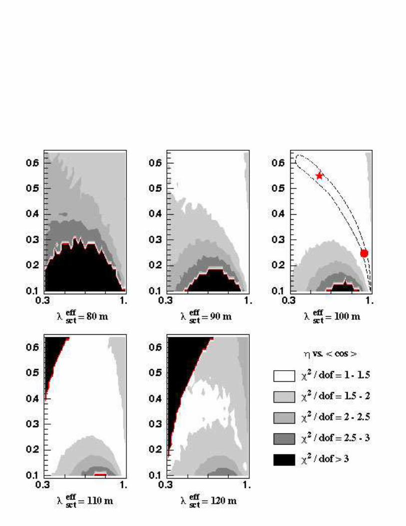
dot position star position
λsct = 30 m λsct = 76 m
η = 0.25 η = 0.56
〈cos〉P = 0.924 〈cos〉P = 0.54
Table 4Scattering parameters at two locations of the degeneracy valley indicated with adot and a star respectively in figure 15.
correlation coefficients between the various scattering parameters :
λabs λmsct λp
sct 〈cos〉p
λabs 1 −0.19 −0.12 −0.08
λmsct 1 −0.87 −0.96
λpsct 1 −0.84
〈cos〉p 1
. (17)
The plots of figure 15 show the existence of a χ2 minimum as a function ofλeff
sct, here found for λeffsct ∼ 100 m, but indicate large degeneracy between η
and 〈cos θ〉 (region delimited by the dashed line). For instance, the dot andthe star shown in these plots have radically different scattering parameters (cf.table 4), although the time distributions for either set of parameters are almostindistinguishable. This follows from identical scattering angle distributionsexcept for small angles (less than ∼30 degrees) to which the experiment ispoorly sensitive.
Available as a separate figure : EtaMcEff NB.jpg
Fig. 15. η vs. 〈cos〉 for various slices in λeffsct. The various shades of grey separate
equidistant regions with a difference of 0.5 in the normalised χ2 per degrees offreedom. The dashed line delimits the 1σ valley. The dot and the star correspondto the scattering parameters in table 4.
This degeneracy in the description of the scattering properties explains the useof the widely cited scattering measurements of Petzold [14] for the particulatescattering phase function, only allowing η, the fraction of molecular to totalscattering, to vary.
4.5 Discussion on systematic uncertainties
Several sources of systematic uncertainties may affect the results of the anal-ysis. These include the slight anisotropy of the source (see section 2.2), an
26

uncertainty in the noise determination (see section 4.1), the reproducibility ofthe source intensity at a given voltage for the simultaneous fit of time distri-butions recorded several hours apart (for the two source-detector distances),the knowledge of the time resolution of the source (time distribution in theabsence of scattering, measured in the lab, cf. section 2.2) and the angulardetection efficiency of the detector module. The systematics that affect therelative normalization of the spectra taken with the two source-detector dis-tances will mostly have an impact on the effective attenuation length and onthe absorption length, while those that change the shape of the spectra willrather affect the scattering length. These systematics are studied with the helpof the Monte Carlo described in section 3.2. An estimate of their effect is givenbelow.
4.5.1 Source anisotropy
To test the impact of the 12% anisotropy of the source, time distributionsare generated with various angular distributions of the light source emission.While the tail of the time distribution is mostly produced by photons havingscattered at large angles, the peak (containing most of the hits) comes fromphotons that have either reached the detector directly or scattered at smallangles, i.e. in either case comes from photons emitted by the portion of thesource facing the detector. Since the relevant information for the determinationof λabs and λeff
att is the relative normalization of the time spectra collected withtwo source-detector distances, which to first order is the relative peak height,and since the source sphere remains in the same position with respect tothe detector for all the measurements, the source anisotropy has a negligibleimpact on the absorption and the effective attenuation lengths. It induces asmall distortion on the tail of the time distributions, however, with an impactof the order of 4% on λsct or λeff
sct.
4.5.2 Noise subtraction
An uncertainty in the noise subtraction will not affect the absorption nor theeffective attenuation lengths since the noise remains small compared to thesignal, and absorption dominates largely over scattering. On the other hand,the scattering length is mostly determined from the tail of the photon arrivaltime distribution, which is barely above noise level. The scattering length istherefore crucially dependent on the precision of the noise subtraction. Fordata taken after June 1999, the spectra have 1100 time bins. The noise contri-bution before the main signal peak is obtained by a fit over more than 500 binswith negligible impact of the uncertainty on the determination of the noise(< 1%). The acquisitions of July 1998 and March 1999, on the other hand,were done with 128 bins only. The noise is therefore estimated from only ∼ 20
27

bins in the worst case (data with the short source-detector distance). The un-certainty on the noise determination can then induce an uncertainty on theeffective scattering length of at most 8%: 16 m, 13 m and 3 m for the July1998, March 1999 and June 2000 blue results respectively, and 1 m for all theresults in UV.
4.5.3 Stability of LED intensity and PMT efficiency
The LED intensity and the PMT efficiency are stable over a given immersion,as was verified by the excellent reproducibility of time spectra taken underthe same conditions up to two hours apart. On two consecutive immersionswith different source-detector distances, however, it is not possible to checkthe stability of the setup. This affects the global normalization of the timespectrum, i.e. the photon collection efficiency (the larger the intensity, thehigher the collection efficiency), and thus the effective attenuation length (seesection 4.3). Depending on the intensity actually used during each immersion,an assumed uncertainty of 1% on the LED intensity and PMT efficiency affectsthe effective attenuation length (and similarly the absorption length) by 1 to11%: 4.5 m, 5.5 m, 1 m and 2 m for the July 1998 (intensity I1), July 1998(intensity I2), March 1999 and June 2000 blue data respectively, 2 m for theJuly 1999 and September 1999 UV data and 1 m for the June 2000 UV data.The impact on the scattering length is negligible since the shape of the timespectrum is unchanged.
4.5.4 Source time distribution
The shape of the time distribution of the source varies with the LED inputvoltage, as illustrated in figure 16. Except for the data recorded in June 2000,time spectra of the source were not always available at the exact same voltageas the one used for the water measurements.
Because the relative normalization of spectra at different source-detector dis-tances is independent of the choice of the source intensity, the effective at-tenuation length, and therefore to first approximation the absorption length,are not affected. The convolution by a slightly different shape of the sourcespectrum does not affect the level of the scattering tail which is set by theeffective scattering length. The latter is therefore also little affected by a poorknowledge of the source time spectrum. The strongest effect appears in thepeak of the distribution, and reflects on the angular dependence of scattering,i.e. on the ratio of molecular to particulate scattering. More quantitatively,the data from July 1999 (taken with a DAC voltage of 5.15 V) are fitted withtwo different source time spectra, first with one at 4.75 V then with one at5.5 V. The absorption length is unchanged, the effective scattering length in-
28

0
0.02
0.04
0.06
0.08
0.1
0.12
0.14
0.16
665 667.5 670 672.5 675 677.5 680 682.5 685 687.5 690delay (ns)
Fig. 16. Normalised time spectra of the UV source for DAC voltages of 4.75V (solidcurve), 5V (dashed curve) and 5.5V (dotted curve).
creases by 6 m between the two fits and η increases by 0.06. Extrapolatingthese results to the difference between the voltage used under water and theone used for the measurement of the source spectrum yields an uncertainty of3 m for the July 1998 and March 1999 blue data and of 1.2 m and 2.4 m forthe July 1999 and September 1999 UV data respectively. There is no effecton the June 2000 blue or UV results since the same source voltage is used forcalibration and data taking.
4.5.5 Angular acceptance of the detector sphere
The angular detection efficiency (studied in [22]) of the glass sphere housingthe photomultiplier tube was simulated under the assumption of the exactknowledge of various factors, some of which are affected by large uncertaintiesas for instance the thickness of the photocathode, the thickness of the opti-cal gel which ensures the optical contact between the photocathode and theglass sphere, or the complex refractive index of the photocathode. The largestchanges in the shape of the efficiency curve are obtained by considering thesmallest (respectively largest) value of the complex refractive index within itspossible range (1.10 + 1.70i to 2.75 + 2.50i), together with the smallest (resp.largest) value of the photocathode thickness (between 16.4 nm and 26.5 nm).Both of these configurations are shown in figure 17.
29

0 10 20 30 40 50 60 70 80 900
0.002
0.004
0.006
0.008
0.01
0.012
0.014
0.016
0.018
0.02
0.022
Model b
Model a
Simulation model
zenithal angle (°)
Detectionefficiency
Fig. 17. Extreme models of the detector sphere angular efficiency (arbitrary units).The solid curve uses a parameterisation of the Moorhead and Tanner data [15] andis the model used in the simulation of the experimental setup. Model a (resp. modelb) uses the thinnest (resp. the thickest) of the photocathodes together with thesmallest (resp. the largest) complex refractive index.
From figure 17 it can be seen that a change in the parameters mentioned abovereflects upon the ratio n<45◦/n>45◦ of photons detected at angles smaller orlarger than about 45◦, where the efficiency shows a local enhancement. Withmodel a on the one hand, this ratio decreases, causing more photons to bedetected at large angles and therefore requiring a larger scattering length toreproduce the light transmission data. Model b on the other hand requires ashorter scattering length. In both cases, the effect is of the order of 8% on theeffective scattering length.
4.5.6 Summary of systematic uncertainties
The total effect of the systematic uncertainties mentioned above is summarisedin tables 5 and 6, adding all the systematic errors in quadrature.
The systematic error is significantly larger than the statistical error. It resultsin an uncertainty of 5 to 11% on the light transmission parameters. Giventhese uncertainties, the variations with time of the values of the parameters(cf. section 4.3) are reduced to a ∼ 2σ effect. To cope with possible temporalvariations of the light transmission parameters, which in this paper are shownto be small, the ANTARES detector will monitor continuously the opticalproperties at the ANTARES site.
30

Epoch λeffatt(in m) λabs (in m) λeff
sct(in m)
July 1998 60.6 ± 0.4 ± 5 68.6 ± 1.3 ± 5 265 ± 4 ± 28
March 1999 51.9 ± 0.7 ± 1 61.2 ± 0.7 ± 1 228 ± 11 ± 24
June 2000 46.4 ± 1.9 ± 2 49.3 ± 0.3 ± 2 301 ± 3 ± 27
Table 5Summary of the results for the blue data (the first error is the statistical error fromtable 2, and the second the systematic error).
Epoch λeffatt(in m) λabs (in m) λeff
sct(in m)
July 1999 21.9 ± 0.8 ± 2 23.5 ± 0.1 ± 2 119 ± 2 ± 10
Sept. 1999 22.8 ± 0.3 ± 2 25.6 ± 0.2 ± 2 113 ± 3 ± 10
June 2000 26.0 ± 0.5 ± 1 28.9 ± 0.1 ± 1 133 ± 3 ± 12
Table 6Summary of the results for the UV data (the first error is the statistical error fromtable 3, and the second the systematic error).
4.6 Stability over the line height
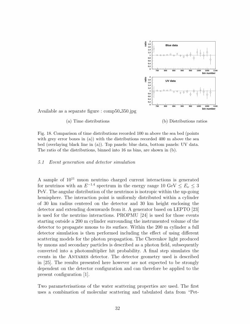
During the immersion of June 2000, data were recorded with distances of100 m and 400 m between the sea bed and the LED source, in both blue andUV, to test for a possible variation of the results with depth. As illustratedin figure 18, the time distributions are fully compatible with one another,whether in blue or in UV, suggesting uniform optical properties along the lineheight. The χ2 between the measurements at the two heights is 297 for 330degrees of freedom for the blue data, and 252 for 324 degrees of freedom forthe UV data.
5 Impact on performance of Antares detector
The primary goal of the Antares detector is to detect high energy muonsproduced by neutrinos interacting around the detector. In this section, weinvestigate the extent to which the detection of muons in Antares will besensitive to the properties of the water (absorption, scattering and angulardistribution) and how the uncertainties in the measurement of these propertieslimit the knowledge of the performance of the detector. Since the effect ofscattering on the time distribution is small, scattering is not expected to havea large impact on the reconstruction efficiency, but it might affect the angularresolution.
31
Available as a separate figure : comp50 350.jpg
(a) Time distributions
00.20.40.60.8
11.21.41.61.8
2
750 800 850 900 950 1000 1050 1100
Blue data
bin number
rati
o
00.20.40.60.8
11.21.41.61.8
2
750 800 850 900 950 1000 1050 1100
UV data
bin number
rati
o
(b) Distributions ratios
Fig. 18. Comparison of time distributions recorded 100 m above the sea bed (pointswith grey error boxes in (a)) with the distributions recorded 400 m above the seabed (overlaying black line in (a)). Top panels: blue data, bottom panels: UV data.The ratio of the distributions, binned into 16 ns bins, are shown in (b).
5.1 Event generation and detector simulation
A sample of 1011 muon neutrino charged current interactions is generatedfor neutrinos with an E−1.4 spectrum in the energy range 10 GeV ≤ Eν ≤ 3PeV. The angular distribution of the neutrinos is isotropic within the up-goinghemisphere. The interaction point is uniformly distributed within a cylinderof 30 km radius centered on the detector and 30 km height enclosing thedetector and extending downwards from it. A generator based on LEPTO [23]is used for the neutrino interactions. PROPMU [24] is used for those eventsstarting outside a 200 m cylinder surrounding the instrumented volume of thedetector to propagate muons to its surface. Within the 200 m cylinder a fulldetector simulation is then performed including the effect of using differentscattering models for the photon propagation. The Cherenkov light producedby muons and secondary particles is described as a photon field, subsequentlyconverted into a photomultiplier hit probability. A final step simulates theevents in the Antares detector. The detector geometry used is describedin [25]. The results presented here however are not expected to be stronglydependent on the detector configuration and can therefore be applied to thepresent configuration [1].
Two parameterisations of the water scattering properties are used. The firstuses a combination of molecular scattering and tabulated data from “Pet-
32

zold” [14] for particle scattering as described in section 3.1. The angular dis-tribution is parameterised by a single parameter η (cf. equation 5). Two suchmodels, P1 and P2, are generated with different values of λsct chosen in therange of observed values (see table 7), with P1 illustrating a conservativecase. The second parameterisation uses a linear combination of two Henyey-Greenstein angular distributions βHG(gi, cos θ) to approximate the total scat-tering angle distribution:
β(cos θ) = α βHG(g1, cos θ) + (1 − α) βHG(g2, cos θ) , (18)
where βHG(g, cos θ) is given by equation 16. The parameters describing theangular distribution are then α (the relative contribution of the two HG func-tions), g1 and g2 (the 〈cos θ〉 of the two HG functions). Five such models,HG1 to HG5, are generated with different values of λsct and 〈cos θ〉.
The simulated models are given in table 7. They have been chosen to includeboth a set of “reasonable” water properties and extreme cases to probe themaximum effect of each parameter. The numbers quoted for these models areat a wavelength corresponding to the blue LED. The wavelength dependenceof the scattering lengths is taken according to the Kopelevich model [20].
Model λsct(m) 〈cos θ〉 λeffsct(m) η α g1 g2
P1 40.8 0.77 175 0.17
P2 52.0 0.77 223 0.17
HG1 52.0 0.77 223 1.000 0.77 0.0
HG2 22.3 0.90 223 1.000 0.90 0.0
HG3 4.4 0.98 223 1.000 0.98 0.0
HG4 40.8 0.90 396 0.985 0.92 -0.6
HG5 52.0 0.90 505 0.985 0.92 -0.6
Table 7Simulated water models and parameters (for λ = 466 nm).
The scattering angle distributions of all seven models are shown in the upperpanel of figure 19. The corresponding time distributions 24 m and 44 m awayfrom the source, as would be measured with the dedicated antares setup(configuration of June 2000 with the blue source), are shown in the lowerpanel. The variety of time distributions is much larger than that actuallyobserved in the data (see for comparison figure 14).
Models P1 and P2 include both molecular and particulate contributions tothe total scattering angle distribution, the molecular part being a major con-tributor to the delayed signal, due to its backscattering component which isas significant as its forward scattering one. The two models only differ by
33

Available as a separate figure : articleDistrib2.jpg
Fig. 19. Top panel: angular distributions β(cos θ) for the models P1, P2, HG1 to HG5described in the text, as well as for pure molecular and pure particulate scatteringdescribed in section 3.1 (grey curves). Bottom panel: time distributions for eachof the models at source-detector distances of 24 m and 44 m (same normalisationprocedure as in figure 7). From top to bottom (better distinction on the second setof curves due to the larger distance of propagation): P1, then P2, then HG1, HG2and HG3 almost indistinguishable from one another, then HG4 and finally HG5.
their scattering lengths. The smaller scattering length of model P1 thereforegenerates the larger tail of delayed photons.
Model HG1 reproduces the same λsct and 〈cos θ〉 as model P2 but with adifferent shape for the scattering angular distribution, as illustrated in theupper panel of figure 19. Its lesser backscattering component causes the cor-responding time distribution to have less delayed photons. In addition, thepeak width is increased. Models HG2 and HG3 have the same λeff
sct as modelHG1 but with different values of 〈cos θ〉, probing the impact of the angulardistribution. With HG1, HG2 and HG3 distributions similarly dominated byforward scattering, it is the effective scattering length that governs the levelsof the tail of delayed photons. The corresponding time distributions are thus,as expected, almost indistinguishable for the three models. Models HG4 andHG5 have the same 〈cos θ〉 as model HG2 but with different λeff
sct. The angulardistribution in models HG4 and HG5 is similar to that of model HG2 withan enhanced backscattering component. The latter is not sufficient howeverto raise significantly the tail of delayed photons and, as can be expected, theincreasing effective scattering lengths lowers the levels of the tail of delayedphotons.
The absorption profile is the same in all cases and corresponds to that in [3]normalised to 62.5 m at 470 nm.
Model P2 is the one that best reproduces the experimental results describedin the previous sections.
5.2 Event reconstruction and analysis
The three-dimensional reconstruction involves several stages of hit selectionsto remove PMT hits due to 40K noise and bioluminescence, as well as severalpre-fits based on plane wave fits through local coincidence and high amplitudehits. The final step is based on a maximum likelihood fit to the distribution ofphoton arrival times with respect to the expected arrival time of Cherenkovlight at a wavelength of 470 nm. The form of the likelihood function is takenfrom an independent Monte Carlo simulation for muons produced by neutri-
34

nos with an E−2 spectrum above 1 TeV. That Monte Carlo includes a 55 meffective attenuation length but neglects scattering so there is no initial as-sumption towards a preferred scattering model. Since the likelihood functionis greatly dominated by the peak where the direct photons were expected, theperformance of the reconstruction is not strongly affected by the shape of thelikelihood function. 10
The performance of the detector is then defined by two figures of merit of thereconstruction:
Angular resolution ∆α defined as the median angle between the MonteCarlo neutrino and the reconstructed track.
Effective volume defined as the fraction of generated events (per bin) whichremain after reconstruction and selection, multiplied by the generation vol-ume.
Both of these quantities are defined after selection cuts which eliminate mis-reconstructed tracks and ensure the purity of the data sample.
5.3 The effect of different water models
The angular resolution as defined above is shown for neutrino energies around1 TeV (0.3 < Eν < 3 TeV) and around 100 TeV (30 < Eν < 300 TeV) foreach of the simulated water models in figure 20 as a function of the individualparameters. Several effects contribute to this resolution. The angle betweenthe muon and neutrino at the interaction vertex decreases with increasingneutrino energy. At 1 TeV, this angle is 0.7◦ on average [25] and is the mostsignificant contribution to the neutrino angular resolution, whereas at highenergies the muon and neutrino are essentially collinear so the accuracy ofreconstructing the muon track dominates the angular resolution. The errorin the event reconstruction contributes an additional error, bringing the res-olution at 1 TeV up to 0.8◦. The scattering increases this further to as muchas 1.2◦, depending on the water model. In the high energy regime, relevantto neutrino astrophysics, the effect of scattering plays a dominant role. For100 TeV, the average muon-neutrino angle is only 0.04◦, the reconstructionbrings it up to 0.20◦ and the scattering further increases it to as much as 0.53◦.
The remarkable agreement between the angular resolutions obtained for mod-els P2 and HG1 implies little sensitivity to the precise shape of the scattering
10 The event reconstruction and selection described here is not optimal for anyspecific analysis. Rather, it is a general approach with no strong assumptions toprovide an unbiased assessment of the effect of different scattering models on theperformance.
35

0 0.05 0.1 0.15 0.2 0.25
reso
luti
on
(d
egre
es)
0
0.2
0.4
0.6
0.8
1
1.2P1
P1
P2
P2
HG1
HG1
HG2
HG2
HG3
HG3
HG4
HG4
HG5
HG5
Angular resolution vs average cos(theta)
0 10 20 30 40 50 60
reso
luti
on
(d
egre
es)
0
0.2
0.4
0.6
0.8
1
1.2P1
P1
P2
P2
HG1
HG1
HG2
HG2
HG3
HG3
HG4
HG4
HG5
HG5
Angular resolution vs scattering length
0 100 200 300 400 500
reso
luti
on
(d
egre
es)
0
0.2
0.4
0.6
0.8
1
1.2P1
P1
P2
P2
HG1
HG1
HG2
HG2
HG3
HG3
HG4
HG4
HG5
HG5
Angular resolution vs effective scattering length
1 1.5 2 2.5 3 3.5 4 4.5 5 5.5 6
Eff
ecti
ve v
olu
me
(km
3 )
10-5
10-4
10-3
10-2
10-1
1
Effective volumes for the ANTARES detector
1- < cos θ > λsct (m)
λsct (m)eff log Eν (GeV)
Fig. 20. Angular resolution for each of the water models as a function of 1−〈cos θ〉,λsct and λeff
sct. The upper points (open circles) correspond to the neutrino resolutionfor 0.3 < Eν < 3 TeV with an E−1.4 spectrum, the lower points (filled circles) for30 < Eν < 300 TeV. The horizontal lines show the angular resolution obtained inthe absence of scattering in each case. The effective volumes are shown for the twomodels with the extreme angular resolutions, HG3 (dashed curve) and HG5 (dottedcurve) and in the absence of scattering (upper solid curve).
angular distribution. Same 〈cos θ〉 and same λeffsct appear to be sufficient to
determine the performance of the detector.
The clearest dependence seen in figure 20 is on the scattering length λsct. Ashorter scattering length degrades the angular resolution. At 1 TeV, the effectof even the most extreme models considered here is at the level of ±12%.It is at high energies where the differences between the water models in theneutrino angular resolution become most significant, at the level of ±30%around the central value.
The effective scattering length λeffsct alone is not enough to describe the effect
of scattering on the angular resolution, as virtually the full range of angularresolutions obtained are seen for a single effective scattering length of 223 m.Similarly, a wide range of values is seen for a single value of 〈cos θ〉 = 0.9.
Given the results of the in-situ measurements (table 2), we can reasonablyestimate 200 < λeff
sct < 400 m and a 〈cos θ〉 ∼ 0.75 for the blue band. Withthis assumption, the variation in angular resolution, even at high energy, is
36

at the level of ±10% around the central value of the angular resolution at0.32◦. Within this, the effect of assuming different angular distributions (withthe same 〈cos θ〉) gives an uncertainty at the level of ±6%. Even for the veryconservative assumption where λsct > 30 m, the uncertainty on the angularresolution only increases to 12%.
The variation in the effective volume of the Antares detector over a widerange of neutrino energies between the extreme models is at the level of ±5%,with models having the worst angular resolutions also yielding the lowesteffective volume (see figure 20).
5.4 Angular resolution of the Antares detector
The present design of the Antares detector comprises a 12-string networkthat will be immersed over the next few years. The event selection can beoptimised in terms of angular resolution and effective volume of the detector.The track is obtained by a 2-stage fit: the position and orientation of the PMTsthat have been hit are used to obtain points that the track is likely to havecrossed. These points are used to obtain an initial track fit. The most probabletrack is then obtained by the minimization of a function involving the residualsof the times at which the Cherenkov photons emitted along the track reach thePMTs of the detector [26]. In the present stage of the reconstruction software,and considering the scattering model that most closely reproduces the datapresented in this paper, model P2 described above, the angular resolution forup-going muon tracks is illustrated in figure 21. For energies Eµ > 300 GeVthe angular resolution for a E−1.4 spectrum is
∆α(µ)= 0.20◦ ± 0.01◦ (stat) ± 0.02◦ (syst) (19)
∆α(ν) = 0.32◦ ± 0.02◦ (stat) ± 0.04◦ (syst) . (20)
The systematics are computed from the study presented in the previous sec-tion.
6 Conclusions
The light transmission at the Antares site has been studied intensively withdedicated setups designed by the collaboration. Absorption and scatteringproperties of the water for blue light (λ = 473 nm) and UV light (λ = 375 nm)were obtained by measuring the distribution of the arrival times of photonsemitted by a pulsed LED source and collected several tens of meters away bya fast photomultiplier tube.
37

log 10 E ν (Gev)
An
gu
lar
reso
luti
on
(d
eg.) 0 < θν < 90
0
0.2
0.4
0.6
0.8
1
1.2
1.4
1.6
1.8
2
2 2.5 3 3.5 4 4.5 5 5.5 6
νµ
Resolutiondominated byphysical θνµ
Resolutiondominated byreconstruction
Fig. 21. Angular resolution (for scattering model P2) as a function of the neutrinoenergy for the reconstruction of the muon track (lower curve) or that of the parentneutrino (upper curve) for a 10-string detector.
The group velocity of light is found in good agreement with predictions fromanalytical models. The absorption length is seen to vary slightly in time, withtypical values of 60 m in blue and 25 m in UV. These values allow a largeeffective area (∼ 0.1 km2 for neutrino-induced muons with energies in the PeVrange) for the planned 12-string Antares detector. With the angular distri-bution of scattering modelled following the standard approach of oceanogra-phers, the scattering length λsct can be extracted with good confidence fromthe data, yielding an effective scattering length λeff
sct = λsct/(1 − 〈cos θ〉) of∼ 260 m in blue and ∼ 120 m in UV. The various parameters describing thelight transmission properties are affected by a 5 to 11% uncertainty, dominatedby systematics. Given these large scattering lengths, an angular resolution of0.3◦ should be achieved for Eµ > 300 GeV, according to the present statusof the reconstruction software. The uncertainty in the knowledge of the waterproperties (due for instance to the observed variations) affects our knowledgeof the angular resolution and effective volume of the detector by 10% and 5%respectively.
The light transmission properties were checked to be constant at a given timeat the two extreme levels (100 m and 400 m above the sea floor) of the activepart of a detector line.
The water properties will be monitored with in-situ dedicated instrumentsduring the lifetime of the Antares detector so that the instantaneous valueswill be available for use in the muon reconstruction software.
38

References
[1] E. Aslanides et al. (Antares Collaboration), preprint CPPM-P-1999-02,DAPNIA 99-01, IFIC/99-42, SHEF-HEP/99-06
[2] Amram, P. et al. (Antares collaboration), Astropart. Phys. 19, 253-267 (2003)
[3] P.B. Price, Appl. Optics 36 (1997) 1965
[4] J.R.V. Zaneveld, in Proceedings of the 1980 International DUMANDSymposium, Vol I, V.J. Stenger ed. (Hawaii DUMAND Center, Honolulu, 1981),pp. 1-8
[5] S.A. Khanaev and A.F. Kuleshov, 2nd NESTOR International Workshop, L.K.Resvanis ed., October 19-21, 1992, pp. 253-269; E.G. Anassontzis, 3nd NESTORInternational Workshop, L.K. Resvanis ed., October 19-21, 1993, pp. 614-630
[6] I.A. Belolaptikov et al, Sixth International Workshop on Neutrino Telescopes,M. Baldo Ceolin ed., Venice, February 22-24, 1994
[7] T.I. Cuickenden and J.A. Irvin, J. Chem. Phys. 72 (1980) 441
[8] L.P. Boivin et al, Appl. Opt. 25 (1986) 877
[9] F.M. Sogandares and S. Fry, Appl. Opt. 36 (1997) 8699
[10] R.M. Pope and E. S. Fry, Appl. Opt. 36 (1997) 8711
[11] J.T.O. Kirk, Appl. Opt. 38, 3135 (1999)
[12] A. Morel and H. Loisel, Appl. Opt. 37, 4765 (1998)
[13] C.D. Mobley et al., Appl. Opt. 32, 7484 (1993)
[14] T.J. Petzold, SIO Ref 72-78, Scripts Inst. Oceanogr., La Jolla, 79 (1972)
[15] M.E. Moorhead and N.W. Tanner, Nucl. Instrum. Meth. A378, 162 (1996)
[16] Amram, P. et al. (Antares collaboration), Astropart. Phys. 13, 127-136 (2000)
[17] R.C. Millard and G. Seaver, Deep Sea Res., 37, 121 (1990)
[18] X. Quan and E. Fry, Appl. Opt. 34, 18 (1995)
[19] R.W. Austin and G. Halikas, SIO Ref. 76-1, Scripps Inst. Oceanogr., La Jolla,121 (1976)
[20] C. D. Mobley, Light and Water (Radiative Transfer in Natural Water),Academic Press (1994)
[21] A. Morel, chapter 1 in Optical aspects of Oceanography, Academic Press (1974)
[22] W. H. Schuster, PhD thesis, University of Oxford, (2002), available athttp://antares.in2p3.fr/Publications/index.html
39

[23] G. Ingelman, A. Edin and J. Rathsman, Comput. Phys. Commun. 101 (1997)108 [hep-ph/9605286]
[24] P. Lipari and T. Stanev, Phys. Rev. D 44 (1991) 3543
[25] Antares proposal, [astro-ph/9907432]
[26] E. Carmona, 27th International Cosmic Ray Conference (ICRC 2001), 7-15 Aug2001, Hamburg, Germany
40