Embed Size (px)
Citation preview

Bull Math BiolDOI 10.1007/s11538-015-0113-5
ORIGINAL ARTICLE
SIS and SIR Epidemic Models Under Virtual Dispersal
Derdei Bichara1 · Yun Kang2 · Carlos Castillo-Chavez1 ·Richard Horan3 · Charles Perrings4
Received: 18 February 2015 / Accepted: 2 October 2015© Society for Mathematical Biology 2015
Abstract We develop a multi-group epidemic framework via virtual dispersal wherethe risk of infection is a function of the residence time and local environmental risk.This novel approach eliminates the need to define and measure contact rates that areused in the traditional multi-group epidemic models with heterogeneous mixing. Weapply this approach to a general n-patch SIS model whose basic reproduction numberR0 is computed as a function of a patch residence-time matrix P. Our analysis impliesthat the resulting n-patch SIS model has robust dynamics when patches are stronglyconnected: There is a unique globally stable endemic equilibrium when R0 > 1,while the disease-free equilibrium is globally stable when R0 ≤ 1. Our further analy-
B Yun [email protected]
Derdei [email protected]
Carlos [email protected]
Richard [email protected]
Charles [email protected]
1 SAL Mathematical, Computational and Modeling Science Center, Arizona State University,Tempe, AZ 85287, USA
2 Sciences and Mathematics Faculty, College of Letters and Sciences, Arizona State University,Mesa, AZ 85212, USA
3 Department of Agricultural, Food and Resource Economics, Michigan State University, EastLansing, MI 48824, USA
4 School of Life Sciences, Arizona State University, Tempe, AZ 85287, USA
123

D. Bichara et al.
sis indicates that the dispersal behavior described by the residence-time matrix P hasprofound effects on the disease dynamics at the single patch level with consequencesthat proper dispersal behavior along with the local environmental risk can either pro-mote or eliminate the endemic in particular patches. Our work highlights the impactof residence-time matrix if the patches are not strongly connected. Our framework canbe generalized in other endemic and disease outbreak models. As an illustration, weapply our framework to a two-patch SIR single-outbreak epidemic model where theprocess of disease invasion is connected to the final epidemic size relationship.We alsoexplore the impact of disease-prevalence-driven decision using a phenomenologicalmodeling approach in order to contrast the role of constant versus state-dependent Pon disease dynamics.
Keywords Epidemiology · SIS–SIR models · Dispersal · Residence times · Globalstability · Adaptive behavior · Final size relationship
Mathematics Subject Classfication Primary 34D23 · 92D25 · 60K35
1 Introduction
Sir Ronald Ross must be considered the founder of mathematical epidemiology (Ross1911) despite the fact that Daniel Bernoulli (1700–1782) was most likely the firstresearcher to introduce the use of mathematical models in the study of epidemic out-breaks (Bernoulli 1766; Dietz and Heesterbeek 2002) nearly 150years earlier. Rossappendix to his 1911 paper (Ross 1911) not only introduces a nonlinear system of dif-ferential equations aimed at capturing the overall dynamics of the malaria contagion,a disease driven by the interactions of hosts, vectors and the life history of Plasmod-ium falciparum, but also includes a tribute to mathematics through his observationthat this framework may also be used to model the dynamics of sexually transmit-ted diseases (Ross 1911). Ross observation has motivated the use of mathematicsin the study of the impact of human social interaction on disease dynamics (Blytheand Castillo-Chavez 1989; Castillo-Chavez and Busenberg 1991; Castillo-Chavez andHuang 1999; Castillo-Chavez et al. 1996, 1999; Hadeler and Castillo-Chavez 1995;Hethcote and Yorke 1984; Hsu Schmitz 2000a, b, 2007; Yorke et al. 1978). In par-ticular, Ross work introduced the type of framework needed to capture and modifythe dynamics of epidemic outbreaks: new landscapes where public policies could betried and tested without harming anybody, complementing and expanding the rolethat statistics plays in epidemiology. Suddenly scientists and public health expertshad a “laboratory” for assessing the impact of transmission mechanisms, evaluating,a priori, efforts aimed at mitigating or eliminating the deleterious impact of diseasedynamics.
The study of the dynamics of communicable disease in metapopulation, multi-group or age-structure models has also benefitted from the work of Ross. Contactmatrices have been used in the study of disease dynamics to accommodate or cap-ture the dynamics of heterogeneous mixing populations (Anderson and May 1982;Castillo-Chavez et al. 1989; Dietz and Schenzle 1985; Hethcote 2000). The spread
123

SIS and SIR Epidemic Models Under Virtual Dispersal
of communicable diseases like measles, chicken pox or rubella is intimately con-nected to the concept of contact, “effective” contact or “effective” per capita contactrate (Castillo-Chavez et al. 1994; Hethcote 2000), a clear measurable concept in, forexample, the context of sexually transmitted diseases (STDs) or vector-borne diseases.The values used to define a contact matrix emerge from the a priori belief that con-tacts can be clearly defined and measured in any context. Their use in the contextof communicable diseases is based often on relative rankings, the result of observa-tional subjective measures of contact or activity levels. For example, since children arebelieved to have the most contacts per unit of time, their observed activity levels areroutinely used to set a relative contact or activity scale. Traditionally, since school chil-dren are assumed to be the most active, they are used to set the scale with the rest of theage-specific contact matrix usually completed under the assumption of proportionate(weighted random) mixing (albeit other forms of mixing are possible Anderson andMay 1991; Blythe and Castillo-Chavez 1989; Castillo-Chavez and Busenberg 1991;Castillo-Chavez et al. 1989; Dietz and Schenzle 1985; Hethcote 2000 and referencestherein). In short, mixing or contact matrices are used to collect rescaled estimatedlevels of activity among interacting subgroups or age-classes, a phenomenologicalestimation process based on observational studies and surveys (Mossong et al. 2008).Our belief that contact rates cannot, in general, be measured in satisfactory ways fordiseases like influenza, measles or tuberculosis arises from the difficulty of assessingthe average number of contacts per unit of time of children in a school bus or theaverage number of contacts per unit of time that children and adults have with eachother in a classroom or at the library, per unit of time. The issue is further confoundedby our inability to assess what an effective contact is: a definition that may have to betied in to the density of floating virus particles, air circulation patterns, or whether ornot contaminated surfaces are touched by susceptible individuals. In short, definingand measuring a contact or an effective contact turn out to be incredibly challenging(Mossong et al. 2008). That said, experimental methods may be used to estimate theaverage risk of acquiring, for example, tuberculosis (TB) or influenza, to individualsthat spend on the average three hours per day in public transportation, in Mexico Cityor New York City.
In this paper, we propose the use of residence times in heterogeneous environments,as a proxy for “effective” contacts per unit time. Catching a communicable diseasewould of course depend on the presence of infected/infectious individuals (a necessarycondition), the level of “risk” within a given “patch” (crowded bars, airports, schools,work places, etc.) and the time spent in such environment. Risk of infection is assumedto be a function of the time spent in pre-specified environments: risk that may beexperimentally measured. We argue that characterizing a landscape as a collectionof patches defined by risk (public transportation, schools, malls, work place, homes,etc.) is possible, especially if the risk of infection in such “local” environments is inaddition a function of residence times and disease levels. Ranking patch-dependentrisks of infection via the values of the transmission rate (β) per unit of time maytherefore be possible and useful. The reinterpretation of β and the use of residencetimes move us away from the world of models that account for transmission viathe use of differential susceptibility to the world where infection depends on localenvironmental risk.
123
D. Bichara et al.
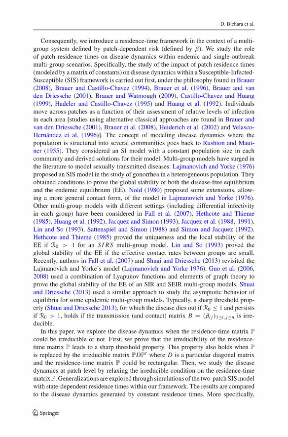
Consequently, we introduce a residence-time framework in the context of a multi-group system defined by patch-dependent risk (defined by β). We study the roleof patch residence times on disease dynamics within endemic and single-outbreakmulti-group scenarios. Specifically, the study of the impact of patch residence times(modeled by amatrix of constants) on disease dynamics within a Susceptible-Infected-Susceptible (SIS) framework is carried out first, under the philosophy found in Brauer(2008), Brauer and Castillo-Chavez (1994), Brauer et al. (1996), Brauer and vanden Driessche (2001), Brauer and Watmough (2009), Castillo-Chavez and Huang(1999), Hadeler and Castillo-Chavez (1995) and Huang et al. (1992). Individualsmove across patches as a function of their assessment of relative levels of infectionin each area [studies using alternative classical approaches are found in Brauer andvan den Driessche (2001), Brauer et al. (2008), Heiderich et al. (2002) and Velasco-Hernández et al. (1996)]. The concept of modeling disease dynamics where thepopulation is structured into several communities goes back to Rushton and Maut-ner (1955). They considered an SI model with a constant population size in eachcommunity and derived solutions for their model. Multi-group models have surged inthe literature to model sexually transmitted diseases. Lajmanovich and Yorke (1976)proposed an SIS model in the study of gonorrhea in a heterogeneous population. Theyobtained conditions to prove the global stability of both the disease-free equilibriumand the endemic equilibrium (EE). Nold (1980) proposed some extensions, allow-ing a more general contact form, of the model in Lajmanovich and Yorke (1976).Other multi-group models with different settings (including differential infectivityin each group) have been considered in Fall et al. (2007), Hethcote and Thieme(1985), Huang et al. (1992), Jacquez and Simon (1993), Jacquez et al. (1988, 1991),Lin and So (1993), Sattenspiel and Simon (1988) and Simon and Jacquez (1992).Hethcote and Thieme (1985) proved the uniqueness and the local stability of theEE if R0 > 1 for an SI RS multi-group model. Lin and So (1993) proved theglobal stability of the EE if the effective contact rates between groups are small.Recently, authors in Fall et al. (2007) and Shuai and Driessche (2013) revisited theLajmanovich and Yorke’s model (Lajmanovich and Yorke 1976). Guo et al. (2006,2008) used a combination of Lyapunov functions and elements of graph theory toprove the global stability of the EE of an SIR and SEIR multi-group models. Shuaiand Driessche (2013) used a similar approach to study the asymptotic behavior ofequilibria for some epidemic multi-group models. Typically, a sharp threshold prop-erty (Shuai and Driessche 2013), for which the disease dies out if R0 ≤ 1 and persistsif R0 > 1, holds if the transmission (and contact) matrix B = (βi j )1≤i, j≤n is irre-ducible.
In this paper, we explore the disease dynamics when the residence-time matrix P
could be irreducible or not. First, we prove that the irreducibility of the residence-time matrix P leads to a sharp threshold property. This property also holds when P
is replaced by the irreducible matrix PDPt where D is a particular diagonal matrix
and the residence-time matrix P could be rectangular. Then, we study the diseasedynamics at patch level by relaxing the irreducible condition on the residence-timematrixP. Generalizations are explored through simulations of the two-patch SISmodelwith state-dependent residence times within our framework. The results are comparedto the disease dynamics generated by constant residence times. More specifically,
123

SIS and SIR Epidemic Models Under Virtual Dispersal
the paper is organized as follows: Sect. 2 introduces a general n patch SIS modelthat accounts for residence times. Theoretical results on the role of residence timesmatrix (P) on disease dynamics are carried out using the residence-time-dependentbasic reproduction number R0(P). The patch-specific reproduction numbers Ri
0(P),i = 1, . . . , n are defined to determine the disease persistence at the patch level. Theusage of R0(P) allows us to explore the cases when the network configuration ofpatches is non-strongly connected. In addition, we also apply our framework to a SImodel and a SIS model without demographics. Section 3 explores, through simula-tions, the dynamics of the SIS model under a state-dependent residence-time matrixin a two-patch system; P ≡ P(I1, I2). That is, when the decisions to spend time ina patch are a function of patch-disease prevalence. Section 4 highlights our frame-work in the case of a two-patch single-outbreak SIR model following the work ofBrauer (2008) and Brauer and Watmough (2009) and discusses the role of P on thefinal epidemic size. Section 5 collects our observations, conclusions and discussesfuture work. The detailed proofs of our theoretical results are provided in the Appen-dix.
2 A General n-Patch SIS Model with Residence Times
A general n-patch SIS model with residence-time matrix P is derived. The globalanalysis of the model is carried out via the basic reproduction number R0. We alsoinclude patch-dependent disease persistence conditions.
2.1 Model Derivation
Wemodel disease dynamicswithin an environment defined by n patches (or risk areas),and so, we let Ni (t), i = 1, 2 . . . , n denote resident population at Patch i at time t . Weassume that Patch i residents spend pi j ∈ [0, 1] time in Patch j , with
∑ j=nj=1 pi j = 1,
for each i = 1, . . . , n. In extreme cases, for example, we may have, for pi j = 0,i �= j , that is Patch i residents spend no time in Patch j while
∑j �=i pi j = 1 (or
equivalently pii = 0) would imply that Patch i residents spend all their time in Patchj (with j = 1, . . . , n and j �= i) even though their patch is (labeled) i . In the absenceof disease dynamics, the population of Patch i residents is modeled by the followingequation:
dNi
dt= bi − di Ni (1)
where the parameters bi and di represent the birth rate and the natural per capita deathrate in Patch i , respectively. Hence, the Patch i resident population approaches theconstant bi
dias t → ∞.
In the presence of disease, we assume that disease dynamics are captured by an SISmodel; thus, the Patch i resident population is divided into susceptible and infectedclasses, represented by Si , Ii , respectively, with Si + Ii = Ni . We further assumethat (a) there is no additional death due to disease; (b) the Patch i infected resident
123

D. Bichara et al.
population recovers and goes back to the susceptible class at the per capita rate γi ; (c)the residence-time matrix P = (pi j )
j=1,...,ni=1,...,n collects the proportion of times spent by
i-residents in j-environments, i = 1, . . . , n and j = 1, . . . , n. The disease dynamicsare therefore described by the following equations:
Si = bi − di Si + γi Ii −n∑
j=1
(Si infected in Patch j)
Ii =n∑
j=1
(Si infected in Patch j) − γi Ii − di Ii
Ni = bi − di Ni . (2)
We model Si infection within Patch j in the following way:
• Since each pi j entry of P denotes the proportion of time that Patch i residentsspent mingling in Patch j , we have that:– There are Ni pi j = Si pi j + Ii pi j Patch i residents in Patch j on the averageat time t .
– The total Patch j , the total effective population is∑n
k=1 Nk pkj , of which∑nk=1 Ik pk j are infected. Hence, the proportion of infected individuals in Patch
j is∑n
k=1 Ik pk j∑nk=1 Nk pk j
and well defined, as long as there exists a k such that pkj > 0,
so that the population in Patch j is nonzero.• Hence, the [Si infected per unit of time in Patch j] can be represented as theproduct of the following three items:
β j︸︷︷︸
the risk of infection in Patch j
× Si pi j︸ ︷︷ ︸
Susceptible from Patch iwho are currently in Patch j
×∑n
k=1 Ik pk j∑nk=1 Nk pkj
︸ ︷︷ ︸Proportion of infected in Patch j
.
The transmission takes on a modified frequency-dependent form that depends onhowmuch time individuals of each epidemiological class spend in a particular area,where β j differs by patch to reflect spatial differences in potential infectivity.Moreprecisely, β j is assumed to be a patch-specific measure of disease risk per unit oftime with its effectiveness tied in to local environmental and sanitary conditions.Therefore,
[Si infected per unit of time in Patch j] ≡ β j × Si pi j ×∑n
k=1 Ik pk j∑nk=1 Nk pkj
(3)
provided that there exists k such that pkj > 0.
123

SIS and SIR Epidemic Models Under Virtual Dispersal
Model (2) can be rewritten as follows:
Si = bi − di Si + γi Ii −n∑
j=1
(
β j × Si pi j ×∑n
k=1 Ik pk j∑nk=1 Nk pkj
)
,
Ii =n∑
j=1
(
β j × Si pi j ×∑n
k=1 Ik pk j∑nk=1 Nk pkj
)
− γi Ii − di Ii ,
Ni = bi − di Ni , (4)
with the dynamics of the Patch i resident total population modeled by the equation:
Ni (t) = bi−di Ni (t), where Si+Ii = Ni , which implies that Ni (t) → bidi
as t → +∞.
Theory of asymptotically autonomous systems for triangular systems (Castillo-Chavezand Thieme 1995; Vidyasagar 1980) guaranties that System (4) is asymptoticallyequivalent to:
Ii =n∑
j=1
(
β j
(bidi
− Ii
)
pi j
∑nk=1 Ik pk j
∑nk=1
bkdkpk j
)
− (γi + di )Ii
= Ii
(bidi
− Ii
)⎛
⎝n∑
j=1
β j p2i j∑n
k=1bkdkpk j
⎞
⎠
+(bidi
− Ii
) n∑
j=1
β j pi j∑n
k=1,k �=i Ik pk j∑n
k=1bkdkpk j
− (di + γi )Ii (5)
for i = 1, 2, . . . , n, with residence-time matrix P = (pi j) j=1,...,ni=1,...,n satisfying the
conditions:HP1 At least one entry in each column of P is strictly positive; andHP2 The sum of all entries in each row is one; i.e.,
∑nj=1 pi j = 1 for all i .
Remarks on Model (5):
1. Timescales: We assume that the disease dynamics occurs at the comparabletimescale as to the demographic dynamics and individuals enter or leave the patchesat the relative faster timescale, e.g., daily or even hourly. The case when there isno demographics in the context of a single epidemic outbreak scenario, has beenconsidered in Sect. 4.
2. In our current modeling framework, we assume that the residence-time matrix P isa n×n matrix. This approach could generalize the concept of k social groups and lpatches by letting n = max{k, l}, pi j |i>k = 0 and pi j | j>l = 0. The consequenceof this generalization is that P could have zero rows (when k < l = n) or columns(when l < k = n). The alternative treatment has been provided in the subsection2.3 (thanks to the referee).
3. We do not assume that the residence-time matrix P being irreducible, instead, weassume that it satisfies relaxed conditions HP1–HP2. More specifically, we will
123
D. Bichara et al.
explore the following two cases: (1) the global dynamics of Model (5) when theresidence-time matrix P is irreducible; (2) the persistence of disease dynamicsat the patch level under conditions of HP1 and HP2 in the following subsectionwhich includes the scenario when P is not irreducible.
2.2 Equilibria, the Basic Reproduction Number and Global Analysis
To analyze the system,we investigate the basic reproduction number of the systemwithfixed residence times to better understand its properties in the absence of behavioralresponses to risk. We let B = (β1, β2, . . . , βn)
t define the risk of infection vector; βiis a measure of the risk per susceptible per unit of time while in residence in Patch i .
Letting S = (S1, S2, . . . , Sn)t , I = (I1, I2, . . . , In)
t , N =(b1d1
,b2d2
, . . . ,bndn
)t
,
and N = Pt N =
⎛
⎜⎜⎜⎜⎝
∑nk=1
bkdkpk1
∑nk=1
bkdkpk2
...∑n
k=1bkdkpkn
⎞
⎟⎟⎟⎟⎠
.Then, System (5) can be rewritten in the following
compact (vectorial) form:
I = diag(N − I )Pdiag(B)diag(N )−1Pt I − diag(dI + γI )I (6)
with state space in Rn+. The set � = {I ≥ 0Rn , I ≤ N } is a compact positively
invariant that attracts all trajectories of System (6). This implies that the populationsinvolved are “biologically” well defined since solutions of (6) will converge to andstay in �. We therefore restrict the dynamics of (6) to the compact set �.
The analysis of System (6) is naturally tied in to the basic reproductive numberR0 (Diekmann et al. 1990; Driessche and Watmough 2002); the average number ofsecondary cases produced by an infected individual during its infectious period whileinteracting with a purely susceptible population. R0 is given by (see the detailedformulation in Appendix):
R0 = ρ(−diag(N )Pdiag(B)diag(N )−1Pt V−1) (7)
where V = −diag(dI + γI ), dI = (d1, d2, . . . , dn)t and γI = (γ1, γ2, . . . , γn)
t .The basic reproduction number R0 is used to establish global properties of System
(6). For the relevant literature on global stability for multi-group or metapopulationmodels, see Arino and Driessche (2003), Iggidr et al. (2012), Kuniya and Muroya(2014), Lajmanovich and Yorke (1976), Sattenspiel and Simon (1988) and the refer-ences therein.We define the disease-free equilibrium (DFE) of System (6) as I ∗ = 0Rn
and the endemic equilibrium (when R0 > 1) as I where all components are positive.By using the same approach as in Iggidr et al. (2012) and Lajmanovich and Yorke(1976), we arrive at the following theorem regarding the global dynamics of Model(6).
123

SIS and SIR Epidemic Models Under Virtual Dispersal
Theorem 2.1 (Global dynamics ofModel (6)) Suppose that the residence-timematrixP is irreducible, then the following statements hold:
• If R0 ≤ 1, the DFE I ∗ = 0Rn is globally asymptotically stable. If R0 > 1 the DFEis unstable.
• If R0 > 1, there exists a unique endemic equilibrium I which is GAS.
Remarks The detailed proof of Theorem2.1 is provided in “Appendix 2.”These resultsimply that System (6) is robust; that is, disease outcomes are completely determinedby whether or not the reproduction number R0 is greater or less than one. The resultsof Theorem 2.1 while powerful do not provide easily accessible insights on the impactof the residence matrix P on the levels of infection within each patch.
Direct insights on the effects ofP are derived by focusing on the levels of endemicitywithin each patch. The following two definitions help set the stage for the discussion:
• The basic reproduction number for Patch i in the absence of movement (pii = 1 or∑i �= j pi j = 0), SIS model, is defined as Ri
0 ≡ βidi+γi
, which determines whether
or not the disease will be endemic in Patch i . In short disease will die out ifRi0 ≤ 1
with a unique endemic equilibrium, that is GAS, if Ri0 > 1.
• The basic reproduction number associated with Patch i , under the presence ofmulti-patch residents, is defined as follows:
Ri0(P) =
∑nj=1 β j
(bidipi j)(
pi j∑n
k=1bkdk
pk j
)
di + γi=
∑nj=1 pi jβ j
( (bidi
pi j)
∑nk=1
bkdk
pk j
)
di + γi
= Ri0 ×
n∑
j=1
pi j
(β j
βi
)⎛
⎝
(bidipi j)
∑nk=1
bkdkpk j
⎞
⎠ .
We explore the role that Ri0(P) plays in determining the impact of all residents on
disease dynamics persistence in Patch i in the following theorem.
Theorem 2.2 (The endemicity of disease in Patch i) Assume that the residence-timematrix P satisfies Condition HP1 and HP2 but that some of its entries can be zeros.
• If Ri0(P) > 1, then the disease persists in Patch i .
• If the following conditions hold:
H:pkj = 0 for all k = 1, . . . , n, and k �= i, whenever pi j > 0,
then we have
Ri0(P) = Ri
0 ×n∑
j=1
pi j
(β j
βi
)⎛
⎝
(pi j
bidi
)
∑nk=1
bkdkpk j
⎞
⎠ = Ri0 ×
n∑
j=1
pi j
(β j
βi
)
.
123

D. Bichara et al.
Thus, when ConditionH holds and Ri0 ×∑n
j=1 pi j(
β jβi
)< 1, then endemic levels
of disease cannot be supported in Patch i . That is,
limt→∞ Ii (t) = 0.
Remarks The detailed proof of Theorem 2.2 is provided in “Appendix 3.” The resultsof Theorem 2.2 give insights on the role that the infection risk (measured by B) andthe residence-time matrix (P) have in promoting or suppressing infection. Further,a closer look at the expression of the general basic reproduction number in Patch i ,namely
Ri0(P) = Ri
0 ×n∑
j=1
pi j
(β j
βi
)⎛
⎝
(bidipi j)
∑nk=1
bkdkpk j
⎞
⎠ ,
leads to the following observations:
1. The movement between patches, modeled via residence-time matrix P, can pro-mote endemicity: For example, ifRi
0 = βidi+γi
≤ 1, i.e., there is no endemic diseasein Patch i , then the presence of movement connecting Patch i to possibly all otherpatches can support endemic disease levels in the following ways:• Via the presence of high-risk patches, that is, there exists a patch j such that
β jβi
is large enough. For example, letting pkl = 1/n for all k, l with the total
population in each patch being the same ( bkdk = K for all k; K a constant) then
Ri0(P) = Ri
0
∑nj=1 β j
nβi, and consequently, if
∑nj=1 β j >
nβiRi
0, then Patch i will
promote the disease at endemic levels.• Whenever individuals spend more time in high-risk patches than in low-riskpatches. For example, in the extreme case, pi j = 1with
β jβi
> 1Ri
0, we have that
Ri0(P) > 1, and thus, endemic disease levels in Patch i can be supported. Patch
j ( j = 1, . . . , n and j �= i) can therefore be considered the source and Patchi (i �= j) the sink (Arino 2008; Arino et al. 2005; Arino and Driessche 2003,2006; Kuniya and Muroya 2014; Lajmanovich and Yorke 1976; Sattenspieland Simon 1988; Sattenspiel and Dietz 1995).
2. Under the assumption Ri0 > 1, for an isolated Patch i , conditions that lead to
disease extinction in the same Patch i under the movement can be identified.According to Theorem 2.2, Condition H should be satisfied and so the expressionof Ri
0(P) reduces to
Ri0(P) = Ri
0 ×n∑
j=1
pi j
(β j
βi
)⎛
⎝
(bidipi j)
∑nk=1
bkdkpk j
⎞
⎠ = Ri0 ×
n∑
j=1
pi j
(β j
βi
)
.
123

SIS and SIR Epidemic Models Under Virtual Dispersal
Therefore, the only way to have the value of Ri0(P) be less than one, would be
when the amount of time spent in Patch i is such that∑n
j=1
(β jβi
)pi j < 1
Ri0(P)
.
Therefore, we conclude that the synergy between the residence-time matrix P andthe existence of sufficient low-risk patches (i.e., β j βi ) can suppress a diseaseoutbreak in Patch i .
2.3 Social Groups Versus Patch Environments
Weassume that there are n social groups interacting inm different patch environments.Let pi j be the proportion time of social group i spent at patch environment j , then theresidence-time matrix P = (pi j ) 1≤i≤n
1≤ j≤mis a n × m matrix.
Following the same modeling approach of the system (5), Model 5 is rewritten asthe following form:
Ii =(bkdk
− Ii
) m∑
j=1
β j pi j
n∑
k=1
Ik pk j
n∑
l=1
bldl
pl j
− (di + γi )Ii
=(bkdk
− Ii
) n∑
k=1
⎛
⎜⎜⎜⎜⎜⎝
m∑
j=1
pi jβ j pk j
n∑
l=1
bldl
pl j
⎞
⎟⎟⎟⎟⎟⎠
Ik − (di + γi )Ii
=(bkdk
− Ii
) n∑
k=1
bik Ik − (di + γi )Ii (8)
where
bik =m∑
j=1
⎛
⎜⎜⎜⎜⎝
pi jβ j pk jn∑
l=1
bldl
pl j
⎞
⎟⎟⎟⎟⎠
.
Model (8) is isomorphic to those considered in Fall et al. (2007), Guo et al.(2006), Guo et al. (2008) and Shuai and Driessche (2013), which could be rewrit-ten in the simplified form (6) as Model (5). Denote the disease transmission matrixB = (bik)1≤i,k≤n , then we also have the form of B = Pdiag(B)diag(N )−1
Pt which
is symmetric. We could see that Theorem 2.1 still holds if the irreducibility of P isreplaced by the irreducibility of B. We should also expect similar results of Theorem2.2 for Model (8) when B is not irreducible.
123

D. Bichara et al.
The difference between the models in the aforementioned papers (e.g., Fall et al.2007; Guo et al. 2006, 2008; Shuai and Driessche 2013) and our model (8) is that: Inthe former models, the disease transmission coefficient βi j involves the contact ratebetween group j and group i ; see the case of bilinear incidence (Guo et al. 2006,2008; Shuai and Driessche 2013) and proportional of βi j for the frequency-dependentincidence (Fall et al. 2007;Guo et al. 2006). In our case, the disease transmissionmatrixB = (bik)1≤i,k≤n is symmetric and incorporates the environmental risks in differentpatches and the proportion of times that different social groups spent in each patch.
Now we apply the approach above to a SIS model without demographics and a SImodel with the disease-induced death rate ci for each social group i as follows.
1. A SIS model without demographics (i.e., assume that the total population size Ni
at each patch i is constant and the natural death rate di = 0) could be rewritten inthe form of:
Ii = Si
n∑
k=1
bik Ik − γi Ii , Si = Ni − Ii (9)
whose simplified form is
I = SBI − GI
where B = (bik)1≤i,k≤n =
⎛
⎜⎜⎜⎜⎝
∑mj=1
⎛
⎜⎜⎜⎜⎝
pi jβ j pk jn∑
l=1
Nl pl j
⎞
⎟⎟⎟⎟⎠
⎞
⎟⎟⎟⎟⎠
1≤i,k≤n
is symmetric, and
G = (γiδik)1≤i,k≤n with δik being the Kronecker delta. The basic reproductionnumber of Model (9) is ρ(BG−1) which determines whether the disease persistsor dies out. Both our Theorems 2.1 and 2.2 could be applied to Model (9)
2. A SI model with the disease-induced death rate ci for each social group i could berewritten in the form of:
Ii = Si
n∑
k=1
bik Ik − ci Ii , Si = Ni − Ii (10)
whose simplified form is
I = SBI − CI
whereC=(ciδik)1≤i,k≤n , and B=(bik)1≤i,k≤n =
⎛
⎜⎜⎜⎜⎝
∑mj=1
⎛
⎜⎜⎜⎜⎝
pi jβ j pk jn∑
l=1
Nl pl j
⎞
⎟⎟⎟⎟⎠
⎞
⎟⎟⎟⎟⎠
1≤i,k≤nis still symmetric but depending on the total population size Nl in each patch.
123

SIS and SIR Epidemic Models Under Virtual Dispersal
Notice that Nl = −cl Il , we expect the total population at each patch approacheszero as time is large enough. This is confirmed by simulations. Simulations alsosuggest that the infection dynamics have similar patterns as the prevalence of theSIR model studied in Sect. 4, and the limit of Ii (t)/Ni (t) goes to 1 for each patchas time is large enough.
3 Two-Patch Models: State-Dependent Residence-Time Matrix
We now extend the analysis of disease dynamics to the case where susceptible indi-viduals respond to variations in risk in an automatic way. In particular, we considerthe case when susceptible individuals make programmed responses to variations indisease risk, and do not choose their response to optimize an index of well-being (see,e.g., Brauer 2008; Brauer et al. 1996; Brauer and van den Driessche 2001; Brauer andWatmough 2009). While this may not be a very good approximation of disease riskmanagement in real systems, it enables us to explore the implications of certain typesof phenomenologically modeled behavioral responses by assuming, for example, thatthe proportion of time spent in a particular patch depends on the numbers of infectedindividuals on that particular patch; that is P ≡ P(I1, I2).
Possible properties of the proportion of time spent by resident of Patch i intoPatch j , i �= j , (pi j ) may include: increases with respect to the growth of infectedresident in Patch i (Ii ) or decreases with respect to infected resident in Patch j (I j ).Mathematically, we would have that
∂pi j (Ii , I j )
∂ I j≤ 0 and
∂pi j (Ii , I j )
∂ Ii≥ 0.
In a two-patch system, the use of the relationship pi j (I1, I2) + p ji (I1, I2) = 1reduces the above four conditions on P to the following conditions:
∂p11(I1, I2)
∂ I1≤ 0 and
∂p22(I1, I2)
∂ I2≤ 0.
Examples of functions pi j (I1, I2) with these properties include,
p12(I1, I2) = σ121 + I1
1 + I1 + I2and p21(I1, I2) = σ21
1 + I21 + I1 + I2
and
p11(I1, I2) = σ11 + σ11 I1 + I21 + I1 + I2
and p22(I1, I2) = σ22 + I1 + σ22 I21 + I1 + I2
where σi j are such that2∑
j=1
σi j = 1.
123

D. Bichara et al.
More complex behavioral response formulations may also depend on the states oftotal populations N1 and N2, but the current specification captures important compo-nents of risk (infections) and allows us to retain the asymptotic equivalence propertyapplied in the case of fixed residence times. Hence, using the same notation as inSystem (6) leads to the following two-dimensional system with P = P(I1, I2):
⎧⎨
⎩
I1 = X (I1, I2)(b1d1
− I1)I1 + Y (I1, I2)
(b1d1
− I1)I2 − (d1 + γ1)I1,
I2 = Y (I1, I2)(b2d2
− I2)I1 + Z(I1, I2)
(b2d2
− I2)I2 − (d2 + γ2)I2,
(11)
where
X (I1, I2) = β1 p211(I1, I2)
p11(I1, I2)b1d1
+ p21(I1, I2)b2d2
+ β2 p212(I1, I2)
p12(I1, I2)b1d1
+ p22(I1, I2)b2d2
,
Y (I1, I2) = β1 p11(I1, I2)p21(I1, I2)
p11(I1, I2)b1d1
+ p21(I1, I2)b2d2
+ β2 p12(I1, I2)p22(I1, I2)
p12(I1, I2)b1d1
+ p22(I1, I2)b2d2
,
and
Z(I1, I2) = β1 p221(I1, I2)
p11(I1, I2)b1d1
+ p21(I1, I2)b2d2
+ β2 p222(I1, I2)
p12(I1, I2)b1d1
+ p22(I1, I2)b2d2
,
where X (I1, I2), Y (I1, I2) and Z(I1, I2) are positive functions of I1 and I2.The basic reproduction number R0 is the same as in the previous section since it is
computed at the infection-free state, i.e.,
R0 = ρ(diag(N )Pdiag(B)diag(N )−1Pt (−V−1))
where, in this case, we have that P =[σ11 σ12σ21 σ22
]
and σi j = pi j (0, 0), ∀{i, j} ={1, 2}.
The properties of positiveness and boundedness of trajectories of System (6) are pre-served in System (11). In addition, System (11) has a unique DFE equilibrium whoselocal stability is determined by the value of theR0: The DFE is locally asymptoticallystable if R0 < 1 while it is unstable if R0 > 1.
Let us considerwhether System (11) canhave a boundary equilibriumsuch as (0, I2)or ( I1, 0). The assumption that System (11) has such a boundary equilibrium (0, I2)with I2 > 0 implies that Y (0, I2) = 0. Since p11(0, I2) = σ11+I2
1+I2and p22(0, I2) =
σ22, we deduce that
Y (0, I2) = β1σ21(σ11 + I2)σ11+I21+I2
b1d1
+ σ21b2d2
(1 + I2)+ β2σ12σ22
σ12b1d1
+ σ22b2d2
(1 + I2).
123

SIS and SIR Epidemic Models Under Virtual Dispersal
This indicates that Y (0, I2) = 0 if and only if σ21 = 0 and σ12 = 0, which requiresthat:
p12 = p21 = 0, and p11 = p22 = 1.
A similar arguments can be applied to the boundary equilibrium ( I1, 0). Therefore, weconclude that System (11) will have a boundary equilibrium
((0, I2) or ( I1, 0)
)only
in the trivial case of isolated patches, that is, where there is no movement between twopatches. This conclusion differs from the state-independent residence matrix model(6), since for example, the two-patch model (6), according to Theorem 2.1, boundaryequilibrium (0, I2) or ( I1, 0) can exist when p11 = p22 = 0 (p12 = p21 = 1).
To illustrate the difference between the state-dependent residence matrix model(11) and the state-independent residence matrix model (6), we look at the situationwhen σ11 = σ22 = 0, σ12 = σ21 = 1 ( p11 = p22 = 0, p12 = p21 = 0 for thestate-independent residence matrix model (6)). Under the condition of σ11 = σ22 =0, σ12 = σ21 = 1, we have Model (11), that
p12(I1, I2) = 1 + I11 + I1 + I2
and p21(I1, I2) = 1 + I21 + I1 + I2
and
p11(I1, I2) = I21 + I1 + I2
and p22(I1, I2) = I11 + I1 + I2
.
This difference has significant impact on disease dynamics (see Fig. 1a, b, red curves).In Fig. 1b, we see that the infection in Patch 2 (high risk) persists in the state-
dependent case, whereas it dies out when P is constant. That is due to the fact thatpii (I1, I2) will not equal zero, whereas pi j (I1, I2) with i �= j may. For the constantresidence-time matrix, the dynamics of the disease in each patch is also independent,where people in Patch i infect only susceptible in Patch j with i �= j . In Fig. 1b (redsolid curve),we observe that the disease dies out in Patch 2with R2
0 = β1d2+γ2
= 0.8571.For the state-dependent case, unless there is no disease in both patches or one disease-free patch, the proportion of time residents spend in their own patch is nonzero. Thisleads the disease to persist in both patches if R0 > 1 (see Fig. 1b, red dashed curves).However, even in this case, the disease dies out in both patches if R0 < 1 (see Fig. 3,red curves, for instance).
3.1 Applications and Comparisons: The Two-Patch Cases
The analytical results of the global dynamics on the asymptotic behavior of Model(11) are still unresolved. Hence, we ran simulations to gain some insights on the roleof P(I1, I2) on endemic dynamics. We observe that trajectories converge toward anendemic equilibrium whenever R0 > 1; however, there are substantial differencesin the transient dynamics generated by state-dependent P(I1, I2) when compared tothose generated with a constant residence-time matrix.
123

D. Bichara et al.
010
2030
4050
6001020304050607080
Tim
e
I 1 Sta
te in
depe
ndan
t res
iden
ce ti
me
I 1 Sta
te d
epen
dant
res
iden
ce ti
me
010
2030
4050
6001020304050607080
Tim
e
I 2 Sta
te in
depe
ndan
t res
iden
ce ti
me
I 2 Sta
te d
epen
dant
res
iden
ce ti
me
(a)
(b)
Fig.1
Cou
pled
dynamicsof
I 1andI 2
forconstant
p ij(solid)andstate-depend
entp i
j(dashed).T
heredlinesiscase
ofhigh
mobility,i.e.,p 1
2=
p 21
=σ12
=σ21
=1.
The
blacklinesrepresentthe
symmetriccase,i.e.,p 1
2=
p 21
=σ12
=σ21
=0.5,andtheblue
line
representthe
polarcase,i.e.,p 1
2=
p 21
=σ12
=σ21
=0.
aDynam
ics
ofthediseasein
Patch1.
Ifthereisno
movem
entbetweenthepatches(bluecurves),thediseasedies
outin
thelow-riskPatch1in
both
approaches
with
R1 0
=0.76
36.b
Dynam
icsof
thediseasein
Patch2.
Inthehigh-m
obility
case,the
diseasedies
out(solid
redcurve)
forPconstant,w
ithR2 0
=0.85
71,and
persistsforPstate-dependent
(dashedredcurve)
(Color
figureon
line)
123

SIS and SIR Epidemic Models Under Virtual Dispersal
0 10 20 30 40 50 600
10
20
30
40
50
60
70
80
Time
I1+I
2 State independant residence time
I1+I
2 State dependant residence time
Fig. 2 Coupled dynamics of I1 + I2 for constant pi j (solid) and state-dependent pi j (dashed). The overallprevalence is higher if the residence times is symmetric (solid and dashed black curves). The black curvesrepresent the symmetric case (p12 = p21 = σ12 = σ21 = 0.5 ), and the blue lines represent the polar case(p12 = p21 = σ12 = σ21 = 0) and red curves represent high-mobility case (p12 = p21 = σ12 = σ21 = 1)(Color figure online)
Unless stated otherwise, we suppose the following generic values for the simu-lations: β1 = 0.3, β2 = 1.2, b1 = 9, d1 = 1/7, b2 = 9, d2 = 1/10 andγ1 = γ2 = 1/4. We carried out numerical simulation for a range of residence-timematrices. It is observed that:
1. For the symmetric case where p12 = p21 = 0.5, the disease is endemic in bothpatches as predicted by Theorem 2.1 since R0 = 2.0466. For the state-dependentcase, simulations suggest (Fig. 1a, b, black dashed curves) that trajectories tendto be endemic in both patches. However, the level of endemicity is lower than theconstant case in Patch 1 (low-risk patch) and is greater in Patch 2 (high-risk patch).
2. Figure 2 sketches the overall prevalence in both patches with three different sce-narios of residence-time matrix P, both the constant and state-dependent case. Thedisease persists since the overall R0 > 1 in all three cases.
3. The case where there is no movement between patches, that is, p12 = p21 =0 (p11 = p22 = 1) and σ12 = σ21 = 0 (or p12(I1, I2) = p21(I1, I2) = 0),corresponds to the case where the system behaves as two isolated patches. In thiscase, the disease dies out or persists in Patch i if Ri
0 is above or below unity inboth approaches. This is illustrated in Fig. 1a, b) where the disease dies out inPatch 1 ( Fig. 1a, blue solid line) where R1
0 = β1d1+γ1
= 0.7636 and the disease
persists in Patch 2 (Fig. 1b, blue solid curve) where R20 = β2
d2+γ2= 3.4286. For
the state-dependent case (dashed blue curves in Fig. 1a, b), the outcome is similarto the constant residence-time case.
4. In Fig. 4a, b, we explore the cases where there is symmetry (σi j = σ j i ) withσi j = pi j (0, 0). We supposed in this case that Patch 2 has higher risk (β2 = 1.2)andPatch 1 has lower risk (β1 = 0.3).As can be intuitively deduced, the prevalencein Patch 1 is at its highest in the case of “high mobility” (σ12 = σ21 = 1), anddecreasing as σi j decreases (with i �= j). Conversely, prevalence in Patch 2 isat its highest under very “low mobility” (σ12 = σ21 = 0) and decreases as σi j
123
D. Bichara et al.
0 10 20 30 40 50 60 70 800
1
2
3
4
5
6
7
8
9
Time
I1
I2
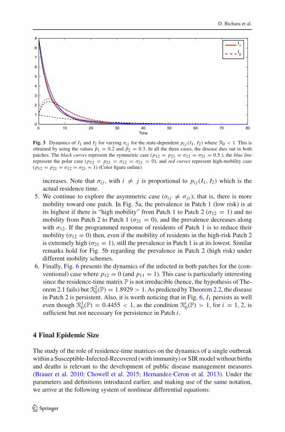
Fig. 3 Dynamics of I1 and I2 for varying σi j for the state-dependent pi j (I1, I2) where R0 < 1. This isobtained by using the values β1 = 0.2 and β2 = 0.3. In all the three cases, the disease dies out in bothpatches. The black curves represent the symmetric case (p12 = p21 = σ12 = σ21 = 0.5 ), the blue linerepresent the polar case (p12 = p21 = σ12 = σ21 = 0), and red curves represent high-mobility case(p12 = p21 = σ12 = σ21 = 1) (Color figure online)
increases. Note that σi j , with i �= j is proportional to pi j (I1, I2) which is theactual residence time.
5. We continue to explore the asymmetric case (σi j �= σ j i ); that is, there is moremobility toward one patch. In Fig. 5a, the prevalence in Patch 1 (low risk) is atits highest if there is “high mobility” from Patch 1 to Patch 2 (σ12 = 1) and nomobility from Patch 2 to Patch 1 (σ21 = 0), and the prevalence decreases alongwith σ12. If the programmed response of residents of Patch 1 is to reduce theirmobility (σ12 = 0) then, even if the mobility of residents in the high-risk Patch 2is extremely high (σ21 = 1), still the prevalence in Patch 1 is at its lowest. Similarremarks hold for Fig. 5b regarding the prevalence in Patch 2 (high risk) underdifferent mobility schemes.
6. Finally, Fig. 6 presents the dynamics of the infected in both patches for the (con-ventional) case where p12 = 0 (and p11 = 1). This case is particularly interestingsince the residence-time matrix P is not irreducible (hence, the hypothesis of The-orem 2.1 fails) butR2
0(P) = 1.8929 > 1. As predicted by Theorem 2.2, the diseasein Patch 2 is persistent. Also, it is worth noticing that in Fig. 6, I1 persists as welleven though R1
0(P) = 0.4455 < 1, as the condition Ri0(P) > 1, for i = 1, 2, is
sufficient but not necessary for persistence in Patch i .
4 Final Epidemic Size
The study of the role of residence-time matrices on the dynamics of a single outbreakwithin a Susceptible-Infected-Recovered (with immunity) or SIRmodel without birthsand deaths is relevant to the development of public disease management measures(Brauer et al. 2010; Chowell et al. 2015; Hernandez-Ceron et al. 2013). Under theparameters and definitions introduced earlier, and making use of the same notation,we arrive at the following system of nonlinear differential equations:
123

SIS and SIR Epidemic Models Under Virtual Dispersal
05
1015
2025
3035
4045
50010203040506070
Tim
e
I1
s 12=
1, s
21=
1, R
0=3.
0545
s 12=
0.8,
s21
=0.
8, R
0=2.
1597
s 12=
0.6,
s21
=0.
6, R
0=2.
0049
s 12=
0.4,
s21
=0.
4, R
0=2.
1459
s 12=
0.2,
s21
=0.
2, R
0=2.
5598
s 12=
0, s
21=
0, R
0=3.
4286
05
1015
2025
3035
4045
50010203040506070
Tim
e
I2
s 12=
1, s
21=
1, R
0=3.
0545
s 12=
0.8,
s21
=0.
8, R
0=2.
1597
s 12=
0.6,
s21
=0.
6, R
0=2.
0049
s 12=
0.4,
s21
=0.
4, R
0=2.
1459
s 12=
0.2,
s21
=0.
2, R
0=2.
5598
s 12=
0, s
21=
0, R
0=3.
4286
(a)
(b)
Fig.4
Dyn
amicsof
I 1andI 2
forvarying
σijforthestate-depend
entp i
j(I 1
,I 2
)approach.a
The
levelo
fprevalence
inPatch1(low
risk)seem
sto
decrease
asσ12
and
σ21
decrease.b
The
levelo
fprevalence
inPatch2(highrisk)seem
sto
increase
asσ12
and
σ21
decrease
(Color
figureon
line)
123

D. Bichara et al.
05
1015
2025
3035
4045
50010203040506070
Tim
e
I1
s 12=
0.9,
s21
=0.
1, R
0=3.
029
s 12=
0.7,
s21
=0.
3, R
0=2.
5378
s 12=
0.5,
s21
=0.
5, R
0=2.
0466
s 12=
0.3,
s21
=0.
7, R
0=1.
5554
s 12=
0.1,
s21
=0.
9, R
0=1.
0642
05
1015
2025
3035
4045
50010203040506070
Tim
e
I2
s 12=
0.9,
s21
=0.
1, R
0=3.
029
s 12=
0.7,
s21
=0.
3, R
0=2.
5378
s 12=
0.5,
s21
=0.
5, R
0=2.
0466
s 12=
0.3,
s21
=0.
7, R
0=1.
5554
s 12=
0.1,
s21
=0.
9, R
0=1.
0642
(a)
(b)
Fig.5
Dyn
amicsof
I 1andI 2
forvarying
σij,but
non-symmetric,forthestate-depend
entp i
j(I 1
,I 2
).aThe
levelo
fprevalence
inPatch1(low
risk)seem
sto
decrease
asσ12
and
σ21
decrease.b
The
levelo
fprevalence
inPatch2(highrisk)seem
sto
increase
asσ12
and
σ21
decrease
(Color
figureon
line)
123

SIS and SIR Epidemic Models Under Virtual Dispersal
0 10 20 30 40 50 600
5
10
15
20
25
30
35
40
45
50
Time
I1
I2
Fig. 6 Dynamics of I1 and I2 where p12 = 0. In this case, the residence-time matrix P is not irreducible,the disease in Patch 2 persists nonetheless as predicted by the Theorem 2.2 (Color figure online)
⎧⎪⎪⎪⎪⎪⎪⎪⎨
⎪⎪⎪⎪⎪⎪⎪⎩
Si = −(
βi p2i iNi pii+N j p ji
+ β j p21i jNi pi j+N j p j j
)
Si Ii −(
βi pii p jiNi pii+N j p ji
+ β j pi j p j jNi pi j+N j p j j
)Si I j ,
Ii =(
βi p2i iNi pii+N j p ji
+ β j p21i jNi pi j+N j p j j
)
Si Ii +(
βi pii p jiNi pii+N j p ji
+ β j pi j p j jNi pi j+N j p j j
)Si I j −αi Ii ,
Ri = αi Ii ,(12)
where Ri denotes the population of recovered immune individuals in Patch i , αi is therecovery rate in Patch i , and Ni ≡ Si + Ii + Ri , for i = 1, 2.
The basic reproduction number R0 is by definition the largest eigenvalue of 2 × 2(n × n for the general case) next-generation matrix,
−FV−1=
⎛
⎜⎜⎜⎝
(β1 p211
N1 p11+N2 p21+ β2 p212
N1 p12+N2 p22
)N1α1
(β1 p11 p21
N1 p11+N2 p21+ β2 p12 p22
N1 p12+N2 p22
)N1α2
(β1 p11 p21
N1 p11+N2 p21+ β2 p12 p22
N1 p12+N2 p22
)N2α1
(β1 p221
N1 p11+N2 p21+ β2 p222
N1 p12+N2 p22
)N2α2
⎞
⎟⎟⎟⎠
.
It has been shown (seeHethcote 1976, for example) that not everybody gets infectedduring an outbreak, and so, estimating the size of the recovered population (the finalepidemic size in the absence of deaths or departures) is tied in the solutions of the finalsize relationship, given in this case, by the system:
⎡
⎢⎣
log S1(0)S1(∞)
log S2(0)S2(∞)
⎤
⎥⎦ =
⎡
⎣K11 K12
K21 K22
⎤
⎦
⎡
⎢⎣
1 − S1(∞)N1
1 − S2(∞)N2
⎤
⎥⎦ (13)
123
D. Bichara et al.
05
1015
2025
30020406080100
120
140
160
180
200
Tim
e
I1
Pre
vale
nce
in P
atch
1
05
1015
2025
30020406080100
120
140
160
180
200
Tim
e
I2
Pre
vale
nce
in P
atch
2
p 11 =
1, p
12 =
0, p
21 =
0, p
22 =
1
p 11 =
0.5
, p12
=0.
5, p
21 =
0.5,
p22
=0.
5
p 11 =
0, p
12 =
1, p
21 =
1, p
22 =
0
p 11 =
1, p
12 =
0, p
21 =
0, p
22 =
1
p 11 =
0.5
, p12
=0.
5, p
21 =
0.5,
p22
=0.
5
p 11 =
0, p
12 =
1, p
21 =
1, p
22 =
0
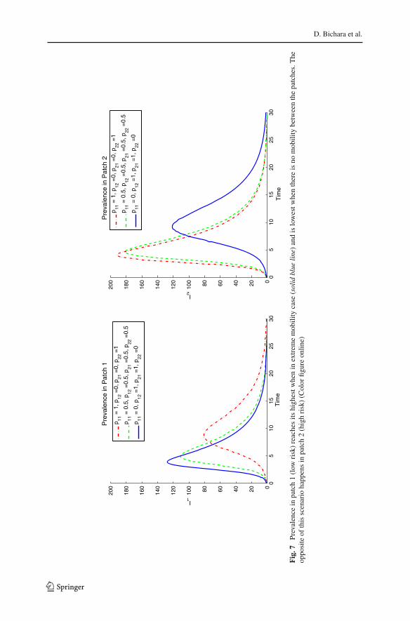
Fig.7
Prevalence
inpatch1(low
risk)reachesits
highestw
henin
extrem
emobility
case
(solid
blue
line)andislowestw
henthereisno
mobility
betweenthepatches.The
oppo
siteof
thisscenario
happ
ensin
patch2(highrisk)(C
olor
figureon
line)
123
SIS and SIR Epidemic Models Under Virtual Dispersal
where
K =
⎡
⎢⎢⎢⎢⎣
(β1 p211
N1 p11+N2 p21+ β2 p212
N1 p12+N2 p22
)N1α1
(β1 p11 p21
N1 p11+N2 p21+ β2 p12 p22
N1 p12+N2p22)
N2α2
(β1 p11 p21
N1 p11+N2 p21+ β2 p12 p22
N1 p12+N2 p22
)N1α1
(β1 p221
N1 p11+p21N2+ β2 p222
N1 p12+N2 p22
)N2α2
⎤
⎥⎥⎥⎥⎦
.
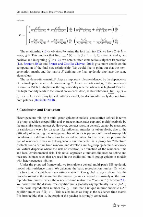
The relationship (13) is obtained by using the fact that, in (12), we have Si + Ii =−αi Ii ≤ 0. This implies that limt→∞ Ii (t) = 0 (for i = 1, 2), since Si and Ii are
positive and integrating SiSi
in (12), we obtain, after some tedious algebra Expression(13). Brauer (2008) and Brauer and Castillo-Chávez (2012) give more details on thecomputation of the final size relationship. We would like to point out that the next-generation matrix and the matrix K defining the final epidemic size have the sameeigenvalues.
The residence-timematrixPplays an important role as evidencedby the dependenceof the final epidemic size relation as in Fig. 7. Aswe can notice in Fig. 7, the prevalencein low-risk Patch 1 is highest in the high-mobility scheme,whereas in high-risk Patch 2,the high mobility leads to the lowest prevalence. Also, as stated before ( lim
t→+∞ Ii (t) =0, for i = 1, 2) with any typical outbreak model, the disease ultimately dies out fromboth patches (Hethcote 2000).
5 Conclusion and Discussion
Heterogeneous mixing in multi-group epidemic models is most often defined in termsof group-specific susceptibility and average contact rates captured multiplicatively bythe transmission parameter β. However, contact rates, in general, cannot be measuredin satisfactory ways for diseases like influenza, measles or tuberculosis, due to thedifficulty of assessing the average number of contacts per unit of time of susceptiblepopulations in different locations for varied activities. In this paper, we propose theuse of residence times in heterogeneous environments, as a proxy for “effective”contacts over a certain time window, and develop a multi-group epidemic frameworkvia virtual dispersal where the risk of infection is a function of the residence timeand local environmental risk. This novel approach eliminates the need to define andmeasure contact rates that are used in the traditional multi-group epidemic modelswith heterogeneous mixing.
Under the proposed framework, we formulate a general multi-patch SIS epidemicmodel with residence times. We calculate the basic reproduction number R0 whichis a function of a patch residence-time matrix P. Our global analysis shows that themodel is robust in the sense that the disease dynamics depend exclusively on the basicreproductive number when the residence-time matrix P is “constant” (Theorem 2.1).We proved that the disease-free equilibrium is globally asymptotically stable (GAS)if the basic reproduction number R0 ≤ 1 and that a unique interior endemic GASequilibrium exists if R0 > 1. This results holds as long as the residence-time matrixP is irreducible; that is, the graph of the patches is strongly connected.
123
D. Bichara et al.
If the residence-time matrix P is not irreducible, that is, the network of the patchesis not strongly connected, Theorem 2.1 does not apply. For these cases, our furtheranalysis (Theorem 2.2) provides accessible insights on the impact of the residencematrix P on the infection levels within each patch. Our results imply that the infectionrisk (measured by B) and the residence-time matrix (P) can play an important rolein the endemicity at the patch level. More specifically, the right combinations of theenvironmental risk level (B) and dispersal behavior (P) can either promote or suppressinfection for particular patches. For example, we are able to apply Theorem 2.2 to thetwo-patch case when residents of Patch 1 visit Patch 2 but not conversely. Theorem 2.2allows us not only to characterize the patch-specific disease dynamics as a functionof the time spend by residents and visitors to the patch of interest, but also to classifypatches as sources or sinks of infection, a role that depends on risk (B) and mobility(P).
The entries of residence-time matrix P could be prevalence dependent, i.e., notconstant anymore. The disease dynamics are expected to be different than the caseswhen P is constant. To explore these differences, we study a two-patch model with thestate-dependent residence-time matrix P, and assume that each entry pi j (I1, I2) of theresidence timesP(I1, I2) is negatively correlated with the prevalence in Patch j .Whenthe residence times P(I1, I2) is prevalence dependent, our analysis and simulationssuggest that (1) its disease dynamics may be prone to persistent by comparing to thecase when P is constant (e.g., Figs. 1, 2); and (2) the disease endemic level could berather complicated (e.g., Figs. 3, 4, 5, 6).
We have extended our framework to a two-patch SIR single-outbreak model toexplore how the residence-time matrix P may affect the final endemic size. We firstderived the final epidemic size relationship in order to capture the size of the outbreak.Our analysis and simulations support that the residence-time matrix P plays an impor-tant role in the final epidemic size. For example, as observed in Fig. 7, the prevalencein low-risk Patch 1 is highest in the high-mobility scheme, whereas in high-risk Patch2, the high mobility leads to the lowest prevalence.
In both conventional and phenomenological approaches to residence times used inthis paper, humans behavior and responses to disease risk are automatic: P is constantand predefined functions of health status. Recent studies (Fenichel et al. 2011; Horanand Fenichel 2007; Horan et al. 2011, 2010; Perrings et al. 2014) have incorporatedbehavior as a feedback response coupled with the dynamics of the disease. Amodel ofthe decision to spend time in patch i = 1, 2 based on individuals’ utility functions thatinclude the possibility of adapting to changing contagion dynamics in the above two-patch setting, using previous work (Fenichel et al. 2011; Morin and Castillo-Chavez2003), is the subject of a separate study.
Acknowledgments These studies were made possible by grant #1R01GM100471-01 from the NationalInstitute of General Medical Sciences (NIGMS) at the National Institutes of Health. The contents of thismanuscript are solely the responsibility of the authors and do not necessarily represent the official viewsof DHS or NIGMS. Research of Y.K. is partially supported by NSF-DMS (1313312). The funders hadno role in study design, data collection and analysis, decision to publish or preparation of the manuscript.The authors are grateful to two anonymous referees for helpful comments and suggestions which led to animprovement of this paper.
123

SIS and SIR Epidemic Models Under Virtual Dispersal
Appendix 1: Computation of R0
Proof The general SIS model with residence time is described by the system (6)
I = diag(N − I )Pdiag(B)diag(N )−1Pt I − diag(dI + γI )I.
The right-hand member of the above system can be clearly decomposed as F + V
where
F = diag(N − I )Pdiag(B)diag(N )−1Pt I and V = −diag(dI + γI )I
The Jacobian matrix at the DFE of F and V is given by:
F=DF
∣∣∣∣DFE
=diag(N )Pdiag(B)diag(N )−1Pt and V =V
∣∣∣∣DFE
=−diag(dI + γI )
The basic reproduction number R0 is given by the spectral radius of the next-generation matrix −FV−1 (Diekmann et al. 1990; Driessche and Watmough 2002).Hence, we deduce that
R0 = ρ(−diag(N )Pdiag(B)diag(N )−1Pt V−1)
�
Appendix 2: Proof of Theorem 2.1
The proof uses the method in Iggidr et al. (2012) which is based on Hirsch’s theorem(Hirsch 1984).
Theorem 5.1 (Hirsch 1984) Let x = F(x) be a cooperative differential equation forwhich R
n+ is invariant , the origin is an equilibrium, each DF(x) is irreducible, andthat all orbits are bounded. Suppose that
x > y �⇒ DF(x) < DF(y) for all x, y.
Then, all orbits in Rn+ tend to zero or there is a unique equilibrium p∗ in the interior
of Rn+ and all orbits in Rn+ tend to p∗.
Proof of Theorem 2.1 Equation (6) can be written as:
I = (F + V )I − diag(I )Pdiag(B)diag(N )−1Pt I (14)
where F = diag(N )Pdiag(B)diag(N )−1Pt and V = −diag(dI + γI ), as defined in
“Appendix 1.” Let us denote by X (I ) the semi-flow induced by (14). Hence,
DX (I ) = diag(N − I )Pdiag(B)diag(N )−1Pt + V − W (I1, I2) (15)
123

D. Bichara et al.
where W (I1, I2) = diag(Pdiag(B)diag(N )−1Pt I ). Since P is irreducible and I ≤
N , DX (I ) is clearly Metzler irreducible matrix. That means, the flow is stronglymonotone. Plus, DX (I ) is clearly decreasing with respect of I . Hence, by Hirsch’stheorem all trajectories either go to zero or go to an equilibrium point I � 0. From therelation (15), we have DX (0) = F +V where F and V are the one defined previouslyin “Appendix 1.” However, since F a nonnegative matrix and V is Metzler, we havethe following equivalence
α(F + V ) < 0 ⇐⇒ ρ(−FV−1) < 1
where α(F + V ) is the stability modulus, i.e., the largest real part of eigenvalues, ofF + V and ρ(−FV−1) the spectral radius of −FV−1. Hence, the DFE is globallyasymptotically stable if R0 = ρ(−FV−1) < 1. And if R0 > 1, i.e., α(F + V ) > 0,the DFE is unstable (Driessche and Watmough 2002). Since, we have proved thatDX (I ) is a Metzler matrix, to prove the local stability of the endemic equilibriumI � 0, we only need to prove that it exists w � 0 such that DX ( I )w < 0 (Bermanand Plemmons 1994). The endemic equilibrium I � 0 satisfies the equation
(F + V ) I − diag( I )Pdiag(B)diag(N )−1Pt I = 0
Hence,
DX ( I ) I = −W ( I ) I < 0
Hence, with w = I , we deduce that I is locally stable. With the attractivity ofI guaranteed Hirsh’s theorem, we conclude that the endemic equilibrium I � 0 isglobally asymptotically stable if R0 > 1.
Finally, ifR0 = 1, we have α(F+V ) = 0. It exists c � 0 such that (F+V )t c = 0.By considering the Lyapunov function V = 〈c|I 〉. This function is definite positiveand its derivation along the trajectories if (14) is
V = ⟨c| I ⟩
=⟨c|(F + V )I − diag(I )Pdiag(B)diag(N )−1
Pt I⟩
= −⟨c|diag(I )Pdiag(B)diag(N )−1
Pt I⟩
≤ 0 (16)
Plus V = 0 only at the DFE. Hence, the DFE is GAS if R0 = 1. This completes theproof of the Theorem 2.1. �
Appendix 3: Proof of Theorem 2.2
Proof Since System (6) has an attracting compact �, then according to Theorem(2.1), we can expect that limt→∞ Ii (t) <
bidi; thus, for time large enough, we can have
bidi
− Ii > 0, therefore we have
123
SIS and SIR Epidemic Models Under Virtual Dispersal
Ii > Ii
(bidi
− Ii
)⎛
⎝n∑
j=1
β j p2i j∑n
k=1 pkjbkdk
⎞
⎠− (di + γi )Ii
which indicates that when Ri0(P) > 1
IiIi
∣∣Ii=0 = bi
di
⎛
⎝n∑
j=1
β j p2i j∑n
k=1 pkjbkdk
⎞
⎠− (di + γi ) > 0.
Then apply the average Lyapunov Theorem (Hutson 1984), we can conclude thatlim inf t→∞ Ii (t) > 0; i.e., the disease in the residence Patch i is persistent ifRi
0(P) >
1 .If pi j > 0 and pkj = 0 for all k = 1, . . . , n, and k �= i , this implies that if there is
a portion of the residence Patch i population flowing into the residence Patch j , thenthere is no other residence Patch k where k �= j , i.e.,
β j pi j
n∑
k=1,k �=i
pk j Ik = 0
which also implies that
(bidi
− Ii
) n∑
j=1
β j pi j∑n
k=1,k �=i pk j Ik∑n
k=1 pkjbkdk
= 0.
then we can conclude that Model (6) can have an equilibrium since under these con-ditions,
bidi
n∑
j=1
β j pi j∑n
k=1,k �=i pk j Ik∑n
k=1 pkjbkdk
= bidi
βi∑n
k=1,k �=i pki Ik∑n
k=1 pkjbkdk
= 0.
Therefore, if the conditions pkj = 0 for all k = 1, . . . , n, and k �= j wheneverpi j > 0 hold, then we have
Ii |Ii=0 =⎡
⎣Ii
(bidi
− Ii
)⎛
⎝n∑
j=1
β j p2i j∑n
k=1 pkjbkdk
⎞
⎠
+(bidi
− Ii
) n∑
j=1
β j pi j∑n
k=1,k �=i pk j Ik∑n
k=1 pkjbkdk
− (di + γi )Ii
⎤
⎦∣∣∣∣Ii=0
= bidi
n∑
j=1
β j pi j∑n
k=1,k �=i pk j Ik∑n
k=1 pkjbkdk
= 0.
123

D. Bichara et al.
Therefore, Ii = 0 is the invariant manifold for Model (6).On the other hand, when these conditions hold, then we have
Ri0(P) = Ri
0 ×n∑
j=1
(β j
βi
)
pi j
⎛
⎝
(pi j
bidi
)
∑nk=1 pkj
bkdk
⎞
⎠ = Ri0 ×
n∑
j=1
(β j
βi
)
pi j .
Therefore, ifRi0(P) = Ri
0 ×∑nj=1
(β jβi
)pi j < 1, then we have the following inequal-
ity:
IiIi
= Ii
(bidi
− Ii
)⎛
⎝n∑
j=1
β j p2i j∑n
k=1 pkibkdk
⎞
⎠− (di + γi )Ii
≤ Ii
⎡
⎣bidi
⎛
⎝n∑
j=1
β j p2i j∑n
k=1 pkibkdk
⎞
⎠− (di + γi )
⎤
⎦
= Ii
⎡
⎣n∑
j=1
β j pi j − (di + γi )
⎤
⎦ < 0.
Therefore, we have limt→∞ Ii (t) = 0; i.e., there is no endemic in the residence Patchi . �
References
Anderson RM, May RM (1982) Directly transmitted infections diseases: control by vaccination. Science215:1053–1060
Anderson RM, May RM (1991) Infectious diseases of humans. Dynamics and control. Oxford SciencePublications, New York
Arino J (2009) Diseases in metapopulations. In: Ma Z, Zhou Y, Wu J (eds) Modeling and dynamics ofinfectious diseases, vol 11. World Scientific, Singapore
Arino J, Davis J, Hartley D, Jordan R,Miller J, van den Driessche P (2005) Amulti-species epidemic modelwith spatial dynamics. Math Med Biol 22:129–142
Arino J, van den Driessche P (2003) The basic reproduction number in a multi-city compartmental model.Lecture notes in control and information science, vol 294, pp 135–142
Arino J, vandenDriesscheP (2006)Disease spread inmetapopulations. In: ZhaoX-O,ZouX (eds)Nonlineardynamics and evolution equations, vol 48. Fields Institute Communications, AMS, Providence, pp 1–13
Berman A, Plemmons RJ (1994) Nonnegative matrices in the mathematical sciences, vol 9 of classicsin applied mathematics. Society for Industrial and Applied Mathematics (SIAM), Philadelphia, PA.Revised reprint of the 1979 original
Bernoulli D (1766) Essai d’une nouvelle analyse de la mortalité causée par la petite vérole, Mem. Math.Phys. Acad. R. Sci. Paris, pp. 1–45
Blythe SP, Castillo-Chavez C (1989) Like-with-like preference and sexual mixing models. Math Biosci96:221–238
Brauer F (2008) Epidemic models with heterogeneous mixing and treatment. Bull Math Biol 70:1869–1885Brauer F, Castillo-Chavez C (1994) Basic models in epidemiology. In: Steele J, Powell T (eds) Ecological
time series. Raven Press, New York, pp 410–477
123

SIS and SIR Epidemic Models Under Virtual Dispersal
Brauer F, Castillo-Chávez C (2012) Mathematical models in population biology and epidemiology. In:Marsden JE, Sirovich L, Golubitski M (eds) Applied mathematics, vol 40. Springer, New York
Brauer F, Castillo-Chavez C, Velasco-Herná ndez JX (1996) Recruitment effects in heterosexually transmit-ted disease models. In: Kirschner D (ed) Advances in mathematical modeling of biological processes,vol 3:1. Int J Appl Sci Comput, pp 78–90
Brauer F, Feng Z, Castillo-Chavez C (2010) Discrete epidemic models. Math Biosci Eng 7:1–15Brauer F, van den Driessche P (2001) Models for transmission of disease with immigration of infectives.
Math Biosci 171:143–154Brauer F, van den Driessche P, Wang L (2008) Oscillations in a patchy environment disease model. Math
Biosci 215:1–10Brauer F, Watmough J (2009) Age of infection epidemic models with heterogeneous mixing. J Biol Dyn
3:324–330Castillo-Chavez C, Busenberg S (1991) A general solution of the problem of mixing of subpopulations and
its application to risk-and age-structured epidemic models for the spread of AIDS. Math Med Biol8:1–29
Castillo-Chavez C, Cooke K, HuangW, Levin SA (1989) Results on the dynamics for models for the sexualtransmission of the human immunodeficiency virus. Appl Math Lett 2:327–331
Castillo-Chavez C, Hethcote H, Andreasen V, Levin S, Liu W (1989) Epidemiological models with agestructure, proportionate mixing, and cross-immunity. J Math Biol 27:233–258
Castillo-Chavez C, Huang W (1999) Age-structured core group modeland its impact on STD dynamics.In Mathematical approaches for emerging and reemerging infectious diseases: models, methods, andtheory (Minneapolis,MN, 1999), vol. 126 of IMA,MathAppl, Springer, NewYork, 2002, pp. 261–273
Castillo-Chavez C, Huang W, Li J (1996) Competitive exclusion in gonorrhea models and other sexuallytransmitted diseases. SIAM J Appl Math 56:494–508
Castillo-Chavez C, Huang W, Li J (1999) Competitive exclusion and coexistence of multiple strains in anSIS STD model. SIAM J Appl Math 59:1790–1811 (electronic)
Castillo-Chavez C, Thieme HR (1995) Asymptotically autonomous epidemic models. In: Arino ADE,Kimmel O, Kimmel M (eds) Mathematical population dynamics: analysis of heterogeneity, volumeone: theory of epidemics. Wuerz, Winnipeg
Castillo-Chavez C, Velasco-Hernández JX, Fridman S (1994) Modeling contact structures in biology. In:Levin SA (ed) Frontiers in mathematical biology, vol 100. Springer, Berlin ch. 454–491
Chowell D, Castillo-Chavez C, Krishna S, Qiu X, Anderson KS (2015) Modelling the effect of earlydetection of Ebola. Lancet 15:148–149
DiekmannO,Heesterbeek JAP,Metz JAJ (1990)On the definition and the computation of the basic reproduc-tion ratio R0 in models for infectious diseases in heterogeneous populations. J Math Biol 28:365–382
Dietz K, Heesterbeek J (2002) Daniel Bernoulli’s epidemiological model revisited. Math Biosci 180:1–21Dietz K, Schenzle D (1985) Mathematical models for infectious disease statistics. In: Atkinson, Anthony,
Fienberg, Stephen E (eds) A celebration of statistics. Springer, New York, pp 167–204Fall A, Iggidr A, Sallet G, Tewa J-J (2007) Epidemiological models and Lyapunov functions. Math Model
Nat Phenom 2:62–68Fenichel E, Castillo-Chavez C, Ceddia MG, Chowell G,Gonzalez Parra P, Hickling GJ, Holloway G, Horan
R, Morin B, Perrings C, Springborn M, Valazquez L, Villalobos C (2011) Adaptive human behaviorin epidemiological models. PNAS 208(15):6306–6311
Guo H, Li M, Shuai Z (2006) Global stability of the endemic equilibrium of multigroup models. Can ApplMath Q 14:259–284
Guo H, Li M, Shuai Z (2008) A graph-theoretic approach to the method of global Lyapunov functions. ProcAm Math Soc 136(8):2793–2802
Hadeler K, Castillo-Chavez C (1995) A core group model for disease transmission. Math Biosci 128:41–55Heiderich KR, Huang W, Castillo-Chavez C (2002) Nonlocal response in a simple epidemiological model.
In: Appli IVM (ed) Mathematical approaches for emerging and reemerging infectious diseases: anintroduction, vol 125. Springer, New York, pp 129–151
Hernandez-Ceron N, Feng Z, Castillo-Chavez C (2013) Discrete epidemic models with arbitrary stagedistributions and applications to disease control. Bull Math Biol 75:1716–1746
Hethcote HW (1976) Qualitative analyses of communicable disease models. Math Biosci 28:335–356Hethcote HW (2000) The mathematics of infectious diseases. SIAM Rev 42:599–653 (electronic)Hethcote HW, Thieme HR (1985) Stability of the endemic equilibrium in epidemic models with subpopu-
lations. Math Biosci 75:205–227
123

D. Bichara et al.
Hethcote HW, Yorke J (1984) Gonorrhea: transmission dynamics and control, vol 56. Lecture notes inbiomathematics. Springer
Hirsch M (1984) The dynamical system approach to differential equations. Bull AMS 11:1–64Horan DR, Fenichel EP (2007) Economics and ecology of managing emerging infectious animal diseases.
Am J Agric Econ 89:1232–1238Horan DR, Fenichel EP, Melstrom RT (2011) Wildlife disease bioeconomics. Int Rev Environ Resour Econ
5:23–61Horan DR, Fenichel EP, Wolf CA, Graming BM (2010) Managing infectious animal disease systems. Annu
Rev Resour Econ 2:101–124Hsu Schmitz S-F (2000a) Effect of treatment or/and vaccination on HIV transmission in homosexual with
genetic heterogeneity. Math Biosci 167:1–18Hsu Schmitz S-F (2000b) A mathematical model of HIV transmission in homosexuals with genetic hetero-
geneity. J Theor Med 2:285–296Hsu Schmitz S-F (2007) The influence of treatment and vaccination induced changes in the risky contact
rate on HIV transmisssion. Math Popul Stud 14:57–76Huang W, Cooke K, Castillo-Chavez C (1992) Stability and bifurcation for a multiple-group model for the
dynamics of HIV/AIDS transmission. SIAM J Appl Math 52:835–854Huang W, Cooke KL, Castillo-Chavez C (1992) Stability and bifurcation for a multiple-group model for
the dynamics of HIV/AIDS transmission. SIAM J Appl Math 52:835–854Hutson V (1984) A theorem on average Lyapunov functions. Monatshefte für Mathematik 98:267–275Iggidr A, Sallet G, Tsanou B (2012) Global stability analysis of a metapopulation SIS epidemic model.
Math Popul Stud 19:115–129Jacquez JA, Simon CP (1993) The stochastic SI model with recruitment and deaths I. Comparison with the
closed SIS model. Math Biosci 117:77–125Jacquez JA, Simon CP, Koopman J (1991) The reproduction number in deterministic models of contagious
diseases. Comment Theor Biol 2:159–209Jacquez JA, SimonCP,Koopman J, Sattenspiel L, PerryT (1988)Modeling and analyzingHIV transmission:
the effect of contact patterns. Math Biosci 92:119–199Kuniya T, Muroya Y (2014) Global stability of a multi-group SIS epidemic model for population migration.
DCDS Ser B 19(4):1105–1118Lajmanovich A, Yorke J (1976) A deterministic model for gonorrhea in a nonhomogeneous population.
Math Biosci 28:221–236Lin X, So JW-H (1993) Global stability of the endemic equilibrium and uniform persistence in epidemic
models with subpopulations. J Aust Math Soc Ser B 34:282–295Morin B, Castillo-Chavez C (2003) SIR dynamics with economically driven contact rates. Nat Resour
Model 26:505–525Mossong J, Hens N, Jit M, Beutels P, Mikolajczyk R, Massari M, Salmaso S, Tomba GS, Wallinga J,
Heijne J, Sadkowska-Todys M, Rosinska M, EdmundsWJ (2008) Social contacts and mixing patternsrelevant to the spread of infectious diseases. PLoS Med 5:381–391
Nold A (1980) Heterogeneity in disease-transmission modeling. Math Biosci 52:227Perrings C, Castillo-Chavez C, Chowell G, Daszak P, Fenichel EP, Finnoff D, Horan RD, Kilpatrick AM,
Kinzig AP, Kuminoff NV, Levin S, Morin B, Smith KF, SpringbornM (2014) Merging economics andepidemiology to improve the prediction and management of infectious disease. Ecohealth 11(4):464–475
Ross R (1911) The prevention of malaria. John Murray, LondonRushton S, Mautner A (1955) The deterministic model of a simple epidemic for more than one community.
Biometrika 42(1/2):126–132Sattenspiel L, Dietz K (1995) A structured epidemic model incorporating geographic mobility among
regions. Math Biosci 128:71–91Sattenspiel L, Simon CP (1988) The spread and persistence of infectious diseases in structured populations.
Math Biosci 90:341–366 [Nonlinearity in biology and medicine (Los Alamos, NM, 1987)]Shuai Z, van den Driessche P (2013) Global stability of infectious disease models using lyapunov functions.
SIAM J Appl Math 73:1513–1532Simon CP, Jacquez JA (1992) Reproduction numbers and the stability of equilibria of SI models for het-
erogeneous populations. SIAM J Appl Math 52:541–576van den Driessche P, Watmough J (2002) Reproduction numbers and sub-threshold endemic equilibria for
compartmental models of disease transmission. Math Biosci 180:29–48
123

SIS and SIR Epidemic Models Under Virtual Dispersal
Velasco-Hernández JX, Brauer F, Castillo-Chavez C (1996) Effects of treatment and prevalence-dependentrecruitment on the dynamics of a fatal disease. IMA J Math Appl Med Biol 13:175–192
Vidyasagar M (1980) Decomposition techniques for large-scale systems with nonadditive interactions:stability and stabilizability. IEEE Trans Autom Control 25:773–779
Yorke JA, Hethcote HW,NoldA (1978) Dynamics and control of the transmission of gonorrhea. Sex TransmDis 5:51–56
123