Single-Phase and Two-Phase Flow Through Orifices in Horizontal PipesThin and Thick

Manmatha K. RoulDepartment of Mechanical Engineering,

Bhadrak Institute of Engineering and Technology,

Bhadrak, India 756113

e-mail: [email protected]

Sukanta K. DashDepartment of Mechanical Engineering,

Indian Institute of Technology,

Kharagpur, India 721302

Single-Phase and Two-PhaseFlow Through Thin and ThickOrifices in Horizontal PipesTwo-phase flow pressure drops through thin and thick orifices have been numericallyinvestigated with air–water flows in horizontal pipes. Two-phase computational fluiddynamics (CFD) calculations, using the Eulerian–Eulerian model have been employed tocalculate the pressure drop through orifices. The operating conditions cover the gas andliquid superficial velocity ranges Vsg¼ 0.3–4 m/s and Vsl¼ 0.6–2 m/s, respectively. Thelocal pressure drops have been obtained by means of extrapolation from the computedupstream and downstream linearized pressure profiles to the orifice section. Simulationsfor the single-phase flow of water have been carried out for local liquid Reynolds number(Re based on orifice diameter) ranging from 3� 104 to 2� 105 to obtain the dischargecoefficient and the two-phase local multiplier, which when multiplied with the pressuredrop of water (for same mass flow of water and two phase mixture) will reproduce thepressure drop for two phase flow through the orifice. The effect of orifice geometry ontwo-phase pressure losses has been considered by selecting two pipes of 60 mm and40 mm inner diameter and eight different orifice plates (for each pipe) with two arearatios (r¼ 0.73 and r¼ 0.54) and four different thicknesses (s/d¼ 0.025–0.59). Theresults obtained from numerical simulations are validated against experimental datafrom the literature and are found to be in good agreement. [DOI: 10.1115/1.4007267]

1 Introduction

The calculation of pressure drop due to gas-liquid two-phaseflow through an orifice is a problem yet to be solved in engineer-ing design. Knowledge of pressure drop for two-phase flowsthrough valves, orifices, and other pipe fittings are important forthe control and operation of industrial devices, such as chemicalreactors, power generation units, refrigeration apparatuses, oilwells, and pipelines. The orifice is one of the most commonlyused elements in flow rate measurement and regulation. Becauseof its simple structure and reliable performance, the orifice isincreasingly adopted in gas-liquid two-phase flow measurements.Single orifices or arrays of them constituting perforated plates, areoften used to enhance flow uniformity and mass distributiondownstream of manifolds and distributors. They are also used toenhance the heat-mass transfer in thermal and chemical processes(e.g., distillation trays). Single-phase flows across orifices havebeen extensively studied, as has been shown by Idelchik et al. [1]in their handbook. The available correlations do not always takeinto account Reynolds number effect and a complete set of geo-metrical parameters. Some investigations have been made on thetheory and experiment of resistance characteristics of orifices[1–7] and some useful correlations have been proposed. However,some of them cover only a limited range of operating conditions,and the errors of some are far beyond the limit of tolerance. Sothey are not widely used in engineering design. Major uncertain-ties exist with reference to two-phase flows through orifices. Fewexperimental studies reported in the literature often refer to alimited set of operating conditions. With particular reference toorifice plates, some of the correlations and models [2–4] are dis-cussed by Friedel [5]. Other references are the early study byJanssen [6] on two-phase pressure loss across abrupt area contrac-tions and expansions taking steam water flow, the work by Lin [7]on two-phase flow measurement with sharp edge orifices; therecent experimental investigation by Saadawi et al. [8], which

refers to two-phase flows across orifices in large diameter pipesand the work by Kojasoy et al. [9] on multiple thick and thinorifice plates. Bertola [10] studied void fraction distribution forair–water flow in a horizontal test section with sudden area con-traction and found that the sudden contraction considerably affectsthe gas distribution in both the upstream and the downstreampipe. Fossa and Guglielmini [11], Fossa et al. [12], and Jones andZuber [13] experimentally investigated two-phase flow pressuredrop through thin and thick orifices and observed that the voidfraction generally increases across the singularity and attains amaximum value just downstream of restriction. Shedd and Newell[14] found a unique set of liquid film thickness and pressure dropdata for horizontal, annular flow of air and water through round,square and triangular tube using a noninvasive, optical liquid filmthickness measurement system.

The information regarding the effects of orifice thickness ontwo-phase pressure losses is not available in the literature. Mostmodels require the knowledge of local void fraction, which is usu-ally calculated by means of correlations for straight pipes withoutorifices and hence the actual void fraction distribution due to ori-fice interactions is not considered. In the present study the effectof orifice geometry on two-phase pressure losses has been consid-ered by selecting two pipes of 60 mm and 40 mm inner diameterand eight different orifice plates (for each pipe) with two arearatios (r¼ 0.73 and r¼ 0.54) and four different thicknesses (threethin and one thick orifice) (s/d¼ 0.025, 0.05, 0.2, 0.59). When thevalue of s/d is below 0.5 it is called a thin orifice otherwise it is athick orifice [3]. The results presented in this study provide usefulinformation on the reliability of available models and correlationswhen applied to intermittent flows through orifices having highvalues of the contraction area ratio.

2 Theoretical Background

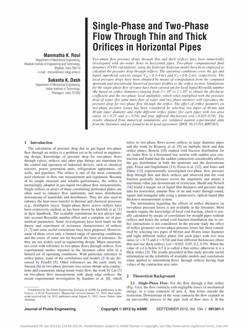
2.1 Single-Phase Flow. For the flow through a thin orifice(Fig. 1(a)), the flow contracts with negligible losses of mechanicalenergy, to a vena contracta of area Ac that forms outside therestriction. Downstream of the vena contracta the flow expands inan irreversible process to the pipe wall of flow area A. If the

Contributed by the Fluids Engineering Division of ASME for publication in theJOURNAL OF FLUID ENGINEERING. Manuscript received January 23, 2012; final manu-script received July 14, 2012; published online August 21, 2012. Assoc. Editor: JohnAbraham.

Journal of Fluids Engineering SEPTEMBER 2012, Vol. 134 / 091301-1Copyright VC 2012 by ASME

Downloaded 09 Jan 2013 to 134.58.253.30. Redistribution subject to ASME license or copyright; see http://www.asme.org/terms/Terms_Use.cfm

orifice is thick (Fig. 1(b)), downstream of the vena contracta, theflow reattaches to the wall within the length of the geometricalcontraction and can even develop a boundary layer flow until itfinally expands back into the pipe wall. According to Chisholm[3], the thick orifice behavior takes place when the dimensionlessorifice thickness to diameter ratio, s/d is greater than 0.5. Assum-ing that each expansion occurs irreversibly and the fluid is incom-pressible, the single-phase pressure drop DPsp in a thin orifice canbe expressed as a function of the flow area ratio r ¼ d=Dð Þ2 andthe contraction coefficient rc ¼ Ac=Ar as

DPsp ¼qV2

2

1

rrc� 1

� �� 2

(1)

where q is the fluid density and V its mean velocity.If the orifice is thick, the loss of mechanical energy is due to

the double expansion as described above. For these conditions thesingle-phase overall pressure drop can be expressed as

DPsp ¼qV2

2

1

rrc

� �2

�1� 2

r2

1

rc� 1

� �� 2

1

r� 1

� �" #(2)

The local pressure drop can also be expressed as a function of ori-fice discharge coefficient Cd (Lin [7], Grace and Lapple [15]),

DPsp ¼qV2

2

1

r

� �2

�1

" #1

C2d

(3)

From Eqs. (1) and (3), rc for thin orifices can be written as

rc;thin ¼1

rþffiffiffiffiffiffiffiffiffiffiffiffiffi1� r2p

=Cd

(4)

Similarly from Eqs. (2) and (3), rc for thick orifices can be written as

rc;thick ¼1

1þffiffiffiffiffiffiffiffiffiffiffiffiffiffiffiffiffiffiffiffiffiffiffiffiffiffiffiffiffiffiffiffiffiffiffiffiffiffiffiffiffiffiffiffiffiffiffiffiffiffiffiffiffiffiffiffiffiffi

1� r2ð Þ=C2d

� �� 1þ 2r� r2

q (5)

The well-known Chisholm expression for contraction coefficientin terms of the area flow ratio only (Chisholm [3], Bullen et al.[16], and Benedict [17]) is given as

rc ¼1

0:639 1� rð Þ0:5þ1h i (6)

In the present study the pressure drops across different orifices forsingle phase flow of water are obtained numerically, from whichthe discharge coefficient is calculated using Eq. (3). The contrac-tion coefficient is calculated using Eqs. (4) and (5) for thin andthick orifices, respectively. This contraction coefficient is com-pared with the Chisholm correlation as given by Eq. (6).

2.2 Two-Phase Flow. According to Chisholm [3] and Morris[4], the slip ratio S is defined as the ratio of gas phase velocity tothe liquid phase velocity at any point in the flow path (Collier andThome [18]) and it is a function of the quality x and the ratio offluid densities. When the quality of mixtures, x is very low (suchas those considered in the present investigation, x< 0.005), theslip ratio, S can be expressed as

S ¼ 1þ xql

qg

� 1

!" #0:5

(7)

The quality, x is defined as the ratio of mass flux of gas to the totalmass flux of mixture at any cross section [18]. The mass flux ofgas is the gas mass flow rate divided by total cross-sectional areaof pipe, whereas the total mass flux is the total mass flow rate ofmixture divided by total cross-sectional area of the pipe. Mathe-matically the quality x can be expressed as

x ¼qggVsg=Across

qggVsg=Across þ qlgVsl=Across

¼qgVsg

qgVsg þ qlVsl(8)

The Armand and Threschev correlation [19] for fully developedflow, near atmospheric pressure, can be expressed in terms of thegas volume fraction xv ¼ Vsg= Vsg þ Vsl

,

S ¼ 1� 0:833xv

0:833 1� xvð Þ (9)

Kojasoy et al. [9] adopted the Chisholm expression for slip ratio Sbut they suggest a correction to account for the effect of flowrestriction on slip ratio,

S ¼ 1þ xql

qg

� 1

!( )0:524

35

n

(10)

The exponent n is zero at the vena contracta and downstream of it(i.e., the slip ratio is expected to be one) while n is equal to 0.4and 0.15 in the upstream region for thin and thick orifices,respectively.

Simpson et al. [2] adopted a different correlation for slip evalu-ation that does not account for the quality of the mixture,

S ¼ ql

qg

!1=6

(11)

The prediction of the two-phase multiplier U2lo can be calculated

using different models as described below. The two-phase multi-plier is defined as the ratio of the two-phase pressure drop throughthe orifice to the single-phase pressure drop obtained at liquidmass flux equal to the overall two-phase mass flux.

If the mixture is considered homogeneous (S ¼ 1), the follow-ing expression can be obtained:

U2lo ¼

ql

qg

xþ 1� xð Þ (12)

Fig. 1 Single-phase flow across (a) thin and (b) thick orifices

091301-2 / Vol. 134, SEPTEMBER 2012 Transactions of the ASME


Chisholm [3] developed the following expression:

U2lo ¼ 1þ ql

qg

� 1

!Bx 1� xð Þ þ x2� �

(13)

where the parameter B can be assumed to be 0.5 for thin orificesand 1.5 for thick ones.

The Morris relationship [4] refers to thin orifices and gatevalves and has the following expression:

U2lo ¼ x

ql

qg

þ S 1� xð Þ" #

xþ 1� x

S

� �1þ S� 1ð Þ2

ql=qg

� �0:5

�1

0B@

1CA

264

375

(14)

where, the slip ratio S is given by Eq. (7).Simpson et al. [2] proposed the following relationship based on

slip predictions given by Eq. (11):

U2lo ¼ 1þ x S� 1ð Þ½ � 1þ x S5 � 1

� �(15)

The Simpson model is based on data collected with large diameterpipes (up to 127 mm) at mixture qualities generally higher thanthose obtained in this work (x< 0.005).

Finally the correlation of Saadawi et al. [8], based on experi-ments carried out at near atmospheric pressure with a very largediameter pipe (203 mm), is given by

U2lo ¼ 1þ 184x� 7293x2 (16)

In the present study the pressure drops across different orifices fortwo-phase flow of air-water mixtures are obtained numerically.The single-phase pressure drops at liquid mass flux equal to theoverall two-phase mass flux are obtained by interpolating thesingle-phase pressure drop results. The two-phase multiplier isobtained by taking the ratio of the two-phase pressure drop to thatof the single phase pressure drop. The two-phase multiplier thusobtained is compared with the theoretical predictions from theabove equations (Eqs. (12)–(16)).

3 Numerical Modeling

The flow field is modeled using the averaged Reynolds equa-tions with realizable per-phase k-e turbulence model, with the twolayer near-wall treatment. The governing equations are brieflydescribed below.

3.1 Governing Equations. Here we considered the two-fluidmethod or Eulerian–Eulerian model, which considers both thephases as interpenetrating continuum, with each computational cellof the domain containing respective fractions of the continuous anddispersed phases. We have adopted the following assumptions in ourstudy which are very realistic for the present situation.

Assumptions:

1. The fluids in both phases are Newtonian, viscous andincompressible.

2. The physical properties remain constant.3. No mass transfer between the two phases.4. The pressure is assumed to be common to both the phases.5. The realizable k-e turbulent model is applied to describe the

behavior of each phase.6. The surface tension forces are neglected; therefore, the pres-

sures of both phases are equal at any cross section.7. The flow is assumed to be isothermal, so the energy equa-

tions are not needed.

With all the above assumptions the governing equations forphase q can be written as (Drew [20], Drew and Lahey [21],Crowe et al. [22]):

Continuity equation:

@

@taqqq

þr � aqqq~vq

¼ 0 (17)

The volume fractions are assumed to be continuous functions ofspace and time and their sum is equal to one

aq þ ap ¼ 1 (18)

Momentum equation:

@

@tðaqqq~vqÞ þ r � aqqq~vq~vq

¼ �aqrpþr � ð��sqÞ þ aqqq~gþMq

(19)

��sq, is the qth phase stress tensor

��sq ¼ aqleffq r~vq þr~vT

q

� �(20)

leffq ¼ lq þ lt;q (21)

where Mq is the interfacial momentum transfer term, which isgiven by

Mq ¼ Mdq þMVM

q þMLq (22)

where the individual terms on the right-hand side of Eq. (22) arethe drag force, virtual mass force, and lift force, respectively. Thedrag force is expressed as

Mdq ¼

3

4dpapqqCD ~vp �~vq

~vp �~vq

(23)

The drag coefficient CD depends on the particle Reynolds numberas given below (Wallis [23]),

CD ¼ 24 1þ 0:15 Re0:687=Rep

� �Rep � 1000

¼ 0:44 Rep> 1000(24)

Particle Reynolds number for primary phase q and secondaryphase p is given by

Rep ¼qq ~vq �~vp

dp

lq

(25)

Equation (23) shows that the drag force exerted by the secondaryphase (bubbles) on the primary phase is a vector directed alongthe relative velocity of the secondary phase. We have varied thediameter of the particle from 10 to 100 micron and have not seenany change in the pressure profile within this range of diameterchange.

The second term in Eq. (22) represents the virtual mass force,which comes into play when one phase is accelerating relative tothe other one. In case of bubble accelerating in a continuous phase,this force can be described by the following expression [20]:

MVMq ¼ �MVM

p ¼ CVMapqq

dq~vq

dt� dp~vp

dt

� �(26)

where CVM is the virtual mass coefficient, which for a sphericalparticle is equal to 0.5 [20].

The third term in Eq. (22) is the lift force, which arises from avelocity gradient of the continuous phase in the lateral directionand is given by Drew and Lahey [21],

MLq ¼ �ML

p ¼ CLapqq ~vp �~vq

� r�~vq

(27)

Journal of Fluids Engineering SEPTEMBER 2012, Vol. 134 / 091301-3


where CL is the lift force coefficient, which for shear flow arounda spherical droplet is equal to 0.5.

Turbulence modeling:Here we considered the realizable per-phase k-e turbulence

model (Launder and Spalding [24], Shih et al. [25], Troshko andHassan [26]).

Transport equations for k:

@

@taqqqkq

þr: aqqq U

!qkq

� �¼ r: aq lq þ

lt;q

rk

� �rkq

� �þ aqGk;q � aqqqeq

þ Kpq Cpqkp � Cqpkq

� Kpq U

!p � U!

q

� �:

lt;p

aprprap

þ Kpq U!

p � U!

q

� �:

lt;q

aqrqraq (28)

Transport equations for e:

@

@taqqqeq

þr: aqqq U

!qeq

� �

¼ r: aq lq þlt;q

re

� �req

� �þ aqqqC1Seq � C2aqqq

e2q

kq þffiffiffiffiffiffiffiffiffiffi�t;qeqp

þ C1eeq

kq

�Kpq Cpqkp � Cqpkq

� Kpq

~Up � ~Uq

�

lt;p

aprprap

þ Kpq~Up � ~Uq

�

lt;q

aqrqraq

�(29)

where ~Uq is the phase-weighted velocity. Here,

C1 ¼ max 0:43;g

gþ 5

� �; g ¼ S

k

e; S ¼ 2SijSij

0:5

The terms Cpq and Cqp can be approximated as

Cpq ¼ 2; Cqp ¼ 2gpq

1þ gpq

!(30)

where gpq is defined as

gpq ¼st;pq

sF;pq(31)

where the Lagrangian integral time scale (st;pq), is defined as

st;pq ¼st;qffiffiffiffiffiffiffiffiffiffiffiffiffiffiffiffiffiffiffiffiffiffiffi

1þ Cbn2

q (32)

where

n ¼~vpq

st;q

Lt;q(33)

where st;q is a characteristic time of the energetic turbulent eddiesand is defined as

st;q ¼3

2Cl

kq

eq(34)

and

Cb ¼ 1:8� 1:35 cos2 h (35)

where h is the angle between the mean particle velocity and themean relative velocity. The characteristic particle relaxation time

connected with inertial effects acting on a dispersed phase p isdefined as

sF;pq ¼ apqqK�1pq

qp

qq

þ CV

!(36)

where CV ¼ 0:5Kpq is defined as the inter phase momentum exchange coeffi-

cient. In flows where there are unequal amounts of two fluids, thepredominant fluid is modeled as the primary fluid, since thesparser fluid is more likely to form droplets or bubbles. Theexchange coefficient for these types of bubbly, liquid-liquid orgas-liquid mixtures can be written in the following general form:

Kpq ¼/q/pqpf

sp

where f, the drag function, is defined differently for the differentexchange-coefficient models and sp, the “particulate relaxationtime,” is defined as

sp ¼qpd2

p

18lq

where dp is the diameter of the bubbles or droplets of phase p.The eddy viscosity model is used to calculate averaged fluctuat-

ing quantities. The Reynolds stress tensor for continuous phase qis given as

sq ¼ �2

3qqkq þ qqlt;qr � ~Uq

I þ qqlt;q r~Uq þr~UT

q

� �(37)

The turbulent viscosity lt;q is written in terms of the turbulent ki-netic energy of phase q,

lt;q ¼ qqClk2

q

eq(38)

The production of turbulent kinetic energy, Gk;q is computed from

Gk;q ¼ lt;q r~vq þr~vTq

� �: r~vq (39)

The production term in the e equation (the second term on theright-hand side of Eq. (29)) does not contain the same Gk term asthe other k-e models. Another desirable feature in the realizablek-e model is that the destruction term (the third term on theright-hand side of Eq. (29)) does not have any singularity, i.e., itsdenominator never vanishes, even if k vanishes or become smallerthan zero. This feature is contrasted with traditional k-e models,which have a singularity due to k in denominator. Unlike standardand RNG k-e models, Cl is not a constant here. It is computedfrom

Cl ¼1

A0 þ AskU�

e

(40)

where

U� �ffiffiffiffiffiffiffiffiffiffiffiffiffiffiffiffiffiffiffiffiffiffiffiffiffiffiffiSijSij þ ~Xij

~Xij

q(41)

and

~Xij ¼ Xij � 2eijkxk

Xij ¼ Xij � eijkxk



where, Xij is the mean rate of rotation tensor viewed in a rotatingreference frame with the angular velocity xk. The constants A0

and As are given by

A0¼ 4:04; As ¼ffiffiffi6p

cos /

where / ¼ 13

cos�1ffiffiffi6p

W

; W ¼ SijSjkSki

S3 , ~S ¼ffiffiffiffiffiffiffiffiffiffiSijSij

p, Sij

¼ 12

@uj

@xiþ @ui

@xj

� �.

The constants used in the model are the following:

C1e¼ 1:44; C2¼ 1:9; rk¼ 1:0; re¼ 1:2

Interphase turbulent momentum transfer:The turbulent drag term Kpq ~vp �~vq

is modeled as follows:

Kpq ~vp �~vq

¼ Kpq

~Up � ~Uq

� Kpq~vdr;pq (42)

Here ~Up and ~Uq are phase-weighted velocities, and ~vdr;pq is thedrift velocity for phase p, which is computed as follows:

~vdr;pq ¼ �Dp

rpqaprap �

Dq

rpqaqraq

� �(43)

The diffusivities Dp and Dq are computed directly from the trans-port equations. The drift velocity results from turbulent fluctua-tions in the volume fraction. When multiplied by the exchangecoefficient Kpq it serves as a correction to the momentumexchange term for turbulent flows.

3.2 Boundary Conditions. Velocity inlet boundary condi-tion is applied at the inlet (as shown in Fig. 2). A no-slip and no-penetrating boundary condition is imposed on the wall of the pipeand the two-layer model for enhanced wall treatment was used toaccount for the viscosity-affected near-wall region. At the outlet,the boundary condition is assigned as outflow, which implies dif-fusion flux for the entire variables in exit direction are zero. Sym-metry boundary condition is considered at the axis, which impliesnormal gradients of all flow variables are zero and radial velocityand the shear stress are zero at the axis.

Boundary conditions for k and e at the inlet are taken as

k ¼ 1

20:02� inlet velocityð Þ2

e ¼ 0:09� k2

10� laminar viscosity

3.3 Near-Wall Treatment. The two-layer model forenhanced wall treatment was used to account for the viscosity-affected near-wall region in numerical computation of turbulentflow. The whole domain is subdivided into a viscosity affectedregion and a fully turbulent region. The demarcation of the tworegions is determined by a wall distance based turbulent Reynoldsnumber, Rey defined as

Rey ¼qy

ffiffiffikp

l(44)

where, y is the normal distance from the wall at the cell centersand it is interpreted as the distance to the nearest wall,

y ¼ min~rw2Cw

~r �~rwk k (45)

where ~r is the position vector at field point, and ~rw is the positionvector on the wall boundary. Cw is the union of all the wall boun-daries involved. This interpretation allows y to be uniquelydefined in flow domains of complex shape involving multiplewalls.

In the fully turbulent region (Rey > Re�y ;Re�y ¼ 200), the k-emodels are employed (Launder and Spalding [24]). In the viscos-ity affected near wall region (Rey < Re�y), the one-equation modelof Wolfstein [27] is employed. In one equation model, themomentum equations and k equation are retained. However, theturbulent viscosity, lt is computed from

lt;2layer ¼ qClllffiffiffikp

(46)

while the rate of dissipation of turbulent kinetic energy e is com-puted from

e ¼ k3=2

le(47)

The length scales ll and le in Eqs. (46) and (47) are computedfrom Chen and Patel [28],

ll ¼ yclð1� e�Rey=AlÞ (48)

le ¼ ycl 1� e�Rey=Ac

� �(49)

Here, the two-layer definition is smoothly blended with the highReynolds number lt definition (as described in the k-e models)from the outer region,

lt;enh ¼ kelt þ ð1� keÞlt;2layer (50)

A blending function ke is defined in such a way that it is equal tounity far from the walls and is zero very near to the walls,

ke ¼1

21þ tanh

Rey � Re�yA

� �� (51)

The constant A determines the width of the blending function. Bydefining a width such that the value of ke will be within 1% of itsfar field value given by a variation of DRey,

A ¼DRey

tanhð0:98Þ (52)

The constants are cl ¼ kC�3=4l ;Al ¼ 70;Ae ¼ 2cl

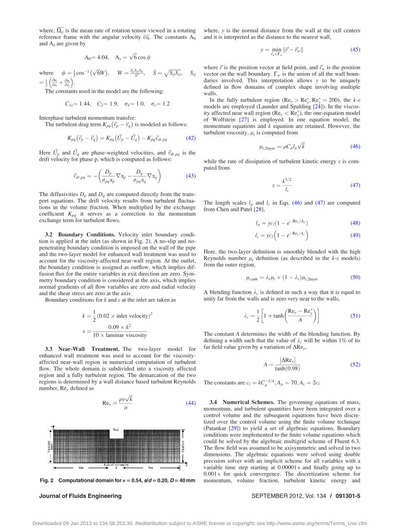
3.4 Numerical Schemes. The governing equations of mass,momentum, and turbulent quantities have been integrated over acontrol volume and the subsequent equations have been discre-tized over the control volume using the finite volume technique(Patankar [29]) to yield a set of algebraic equations. Boundaryconditions were implemented to the finite volume equations whichcould be solved by the algebraic multigrid scheme of Fluent 6.3.The flow field was assumed to be axisymmetric and solved in twodimensions. The algebraic equations were solved using doubleprecision solver with an implicit scheme for all variables with avariable time step starting at 0.00001 s and finally going up to0.001 s for quick convergence. The discretization scheme formomentum, volume fraction, turbulent kinetic energy andFig. 2 Computational domain for r 5 0.54, s/d 5 0.20, D 5 40 mm



turbulent dissipation rate were taken to be first order up windinginitially for better convergence. Slowly as time progressed the dis-cretization forms were switched over to second order up windingand then slowly towards the QUICK scheme for better accuracy.It is to be noted here that in the Eulerian scheme of solution, twocontinuity equations and two momentum equations were solvedfor two phases. The phase-coupled SIMPLE algorithm (Vasquezand Ivanov [30], Ansari and Shokri [31]) which is an extension ofthe SIMPLE algorithm (Patankar [29]) for multiphase flows wasused for the pressure-velocity coupling. The velocities weresolved coupled by the phases, but in a segregated fashion. Theblock algebraic multigrid (AMG) method (Wesseling [32], Weisset al. [33]) was used to solve all the algebraic equations resultingfrom the discretization of the continuity and momentum equationsof all phases simultaneously. Then a pressure correction equationwas built based on total volume continuity rather than mass conti-nuity. Pressure and velocities were then corrected so as to satisfythe continuity constraint. The realizable per-phase k-e model(Shih et al. [25]) has been used as a closure model for turbulentflow. The two-layer model for enhanced wall treatment was usedto account for the viscosity-affected near-wall region in numericalcomputation of turbulent flow. Fine grids were used near the wallas well as near the orifice, where the mean flow changes rapidlyand there are shear layers with a large mean rate of strain. Thescaled residuals for continuity, velocity of water and air in axialand radial directions, k and e for water and air, and volume frac-tion for air were monitored. The convergence criteria for all thevariables were taken to be 0.001. If the residuals for all problemvariables fall below the convergence criteria but are still indecline, the solution is still changing, to a greater or lesser degree.A solution is said to be truly converged if the scaled residuals areno longer changing with successive iterations. A better indicatoroccurs when the residuals flatten in a traditional residual plot (ofresidual value versus iteration). Convergence was judged not onlyby examining scaled residual levels, but also by monitoring thevelocities and pressures at three different locations very close tothe orifice section (at 5D upstream, at the orifice and at 5Ddownstream). The solution was considered to have convergedwhen there was no further observable change in the velocity andpressure at each location. Finally it was observed that the scaledresidual for continuity equation was below 10�3 and that for allother variables were well below 10�6. The convergence criteriawere selected by first solving the problem in transient state andthen it is solved in steady state.

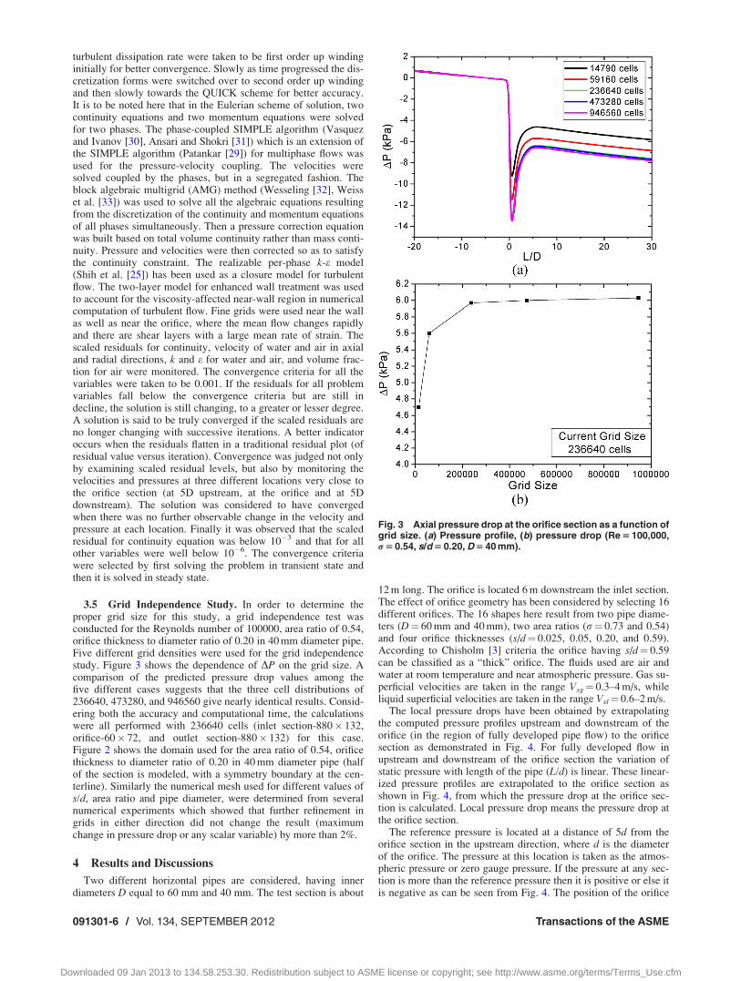
3.5 Grid Independence Study. In order to determine theproper grid size for this study, a grid independence test wasconducted for the Reynolds number of 100000, area ratio of 0.54,orifice thickness to diameter ratio of 0.20 in 40 mm diameter pipe.Five different grid densities were used for the grid independencestudy. Figure 3 shows the dependence of DP on the grid size. Acomparison of the predicted pressure drop values among thefive different cases suggests that the three cell distributions of236640, 473280, and 946560 give nearly identical results. Consid-ering both the accuracy and computational time, the calculationswere all performed with 236640 cells (inlet section-880� 132,orifice-60� 72, and outlet section-880� 132) for this case.Figure 2 shows the domain used for the area ratio of 0.54, orificethickness to diameter ratio of 0.20 in 40 mm diameter pipe (halfof the section is modeled, with a symmetry boundary at the cen-terline). Similarly the numerical mesh used for different values ofs/d, area ratio and pipe diameter, were determined from severalnumerical experiments which showed that further refinement ingrids in either direction did not change the result (maximumchange in pressure drop or any scalar variable) by more than 2%.

4 Results and Discussions

Two different horizontal pipes are considered, having innerdiameters D equal to 60 mm and 40 mm. The test section is about

12 m long. The orifice is located 6 m downstream the inlet section.The effect of orifice geometry has been considered by selecting 16different orifices. The 16 shapes here result from two pipe diame-ters (D¼ 60 mm and 40 mm), two area ratios (r¼ 0.73 and 0.54)and four orifice thicknesses (s/d¼ 0.025, 0.05, 0.20, and 0.59).According to Chisholm [3] criteria the orifice having s/d¼ 0.59can be classified as a “thick” orifice. The fluids used are air andwater at room temperature and near atmospheric pressure. Gas su-perficial velocities are taken in the range Vsg¼ 0.3–4 m/s, whileliquid superficial velocities are taken in the range Vsl¼ 0.6–2 m/s.

The local pressure drops have been obtained by extrapolatingthe computed pressure profiles upstream and downstream of theorifice (in the region of fully developed pipe flow) to the orificesection as demonstrated in Fig. 4. For fully developed flow inupstream and downstream of the orifice section the variation ofstatic pressure with length of the pipe (L/d) is linear. These linear-ized pressure profiles are extrapolated to the orifice section asshown in Fig. 4, from which the pressure drop at the orifice sec-tion is calculated. Local pressure drop means the pressure drop atthe orifice section.

The reference pressure is located at a distance of 5d from theorifice section in the upstream direction, where d is the diameterof the orifice. The pressure at this location is taken as the atmos-pheric pressure or zero gauge pressure. If the pressure at any sec-tion is more than the reference pressure then it is positive or else itis negative as can be seen from Fig. 4. The position of the orifice

Fig. 3 Axial pressure drop at the orifice section as a function ofgrid size. (a) Pressure profile, (b) pressure drop (Re 5 100,000,r 5 0.54, s/d 5 0.20, D 5 40 mm).



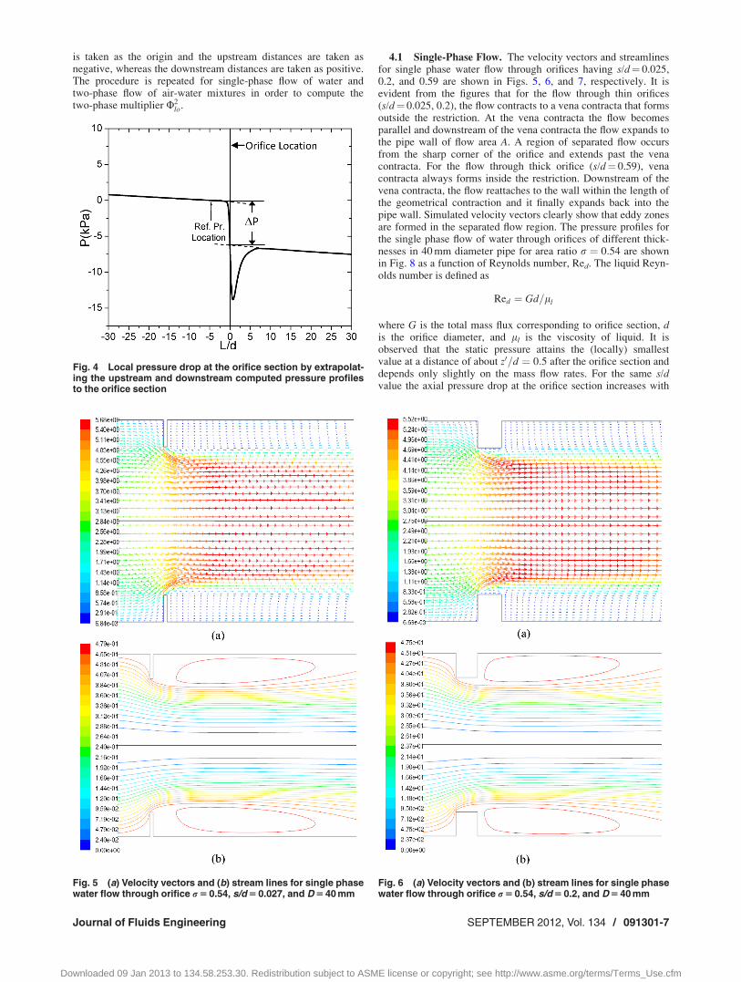
is taken as the origin and the upstream distances are taken asnegative, whereas the downstream distances are taken as positive.The procedure is repeated for single-phase flow of water andtwo-phase flow of air-water mixtures in order to compute thetwo-phase multiplier U2

lo.

4.1 Single-Phase Flow. The velocity vectors and streamlinesfor single phase water flow through orifices having s/d¼ 0.025,0.2, and 0.59 are shown in Figs. 5, 6, and 7, respectively. It isevident from the figures that for the flow through thin orifices(s/d¼ 0.025, 0.2), the flow contracts to a vena contracta that formsoutside the restriction. At the vena contracta the flow becomesparallel and downstream of the vena contracta the flow expands tothe pipe wall of flow area A. A region of separated flow occursfrom the sharp corner of the orifice and extends past the venacontracta. For the flow through thick orifice (s/d¼ 0.59), venacontracta always forms inside the restriction. Downstream of thevena contracta, the flow reattaches to the wall within the length ofthe geometrical contraction and it finally expands back into thepipe wall. Simulated velocity vectors clearly show that eddy zonesare formed in the separated flow region. The pressure profiles forthe single phase flow of water through orifices of different thick-nesses in 40 mm diameter pipe for area ratio r ¼ 0:54 are shownin Fig. 8 as a function of Reynolds number, Red. The liquid Reyn-olds number is defined as

Red ¼ Gd=ll

where G is the total mass flux corresponding to orifice section, dis the orifice diameter, and ll is the viscosity of liquid. It isobserved that the static pressure attains the (locally) smallestvalue at a distance of about z0=d ¼ 0:5 after the orifice section anddepends only slightly on the mass flow rates. For the same s/dvalue the axial pressure drop at the orifice section increases with

Fig. 4 Local pressure drop at the orifice section by extrapolat-ing the upstream and downstream computed pressure profilesto the orifice section

Fig. 5 (a) Velocity vectors and (b) stream lines for single phasewater flow through orifice r 5 0.54, s/d 5 0.027, and D 5 40 mm




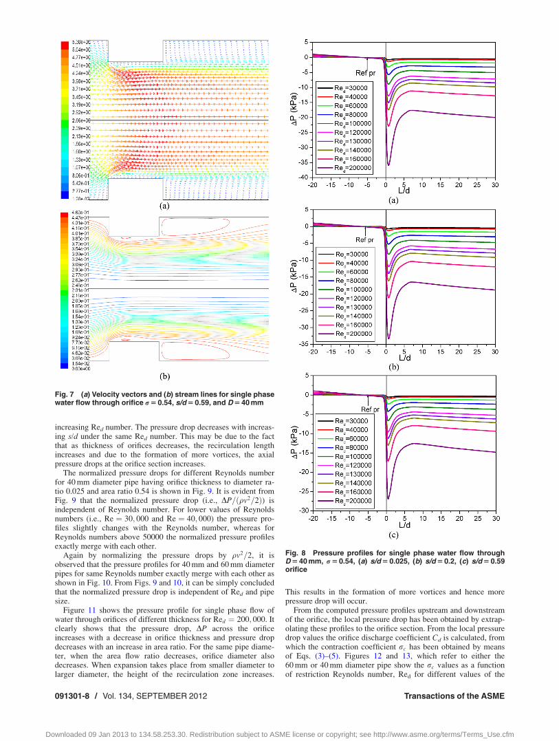
increasing Red number. The pressure drop decreases with increas-ing s/d under the same Red number. This may be due to the factthat as thickness of orifices decreases, the recirculation lengthincreases and due to the formation of more vortices, the axialpressure drops at the orifice section increases.

The normalized pressure drops for different Reynolds numberfor 40 mm diameter pipe having orifice thickness to diameter ra-tio 0.025 and area ratio 0.54 is shown in Fig. 9. It is evident fromFig. 9 that the normalized pressure drop (i.e., DP=ðqv2=2Þ) isindependent of Reynolds number. For lower values of Reynoldsnumbers (i.e., Re ¼ 30; 000 and Re ¼ 40; 000) the pressure pro-files slightly changes with the Reynolds number, whereas forReynolds numbers above 50000 the normalized pressure profilesexactly merge with each other.

Again by normalizing the pressure drops by qv2=2, it isobserved that the pressure profiles for 40 mm and 60 mm diameterpipes for same Reynolds number exactly merge with each other asshown in Fig. 10. From Figs. 9 and 10, it can be simply concludedthat the normalized pressure drop is independent of Red and pipesize.

Figure 11 shows the pressure profile for single phase flow ofwater through orifices of different thickness for Red ¼ 200; 000. Itclearly shows that the pressure drop, DP across the orificeincreases with a decrease in orifice thickness and pressure dropdecreases with an increase in area ratio. For the same pipe diame-ter, when the area flow ratio decreases, orifice diameter alsodecreases. When expansion takes place from smaller diameter tolarger diameter, the height of the recirculation zone increases.

This results in the formation of more vortices and hence morepressure drop will occur.

From the computed pressure profiles upstream and downstreamof the orifice, the local pressure drop has been obtained by extrap-olating these profiles to the orifice section. From the local pressuredrop values the orifice discharge coefficient Cd is calculated, fromwhich the contraction coefficient rc has been obtained by meansof Eqs. (3)–(5). Figures 12 and 13, which refer to either the60 mm or 40 mm diameter pipe show the rc values as a functionof restriction Reynolds number, Red for different values of the


Fig. 8 Pressure profiles for single phase water flow throughD 5 40 mm, r 5 0.54, (a) s/d 5 0.025, (b) s/d 5 0.2, (c) s/d 5 0.59orifice



flow area ratio. It can be observed from Figs. 12 and 13 that thecontraction coefficient turns out to be independent of the Reynoldsnumber for values above 5� 104. For lower values of Reynoldsnumber, the contraction coefficient generally increases with it.Finally it can be noticed that the contraction coefficient data are ingood agreement with Chisholm formula predictions (Eq. (6)). Thecontraction coefficient is high (around 0.8) for 0.73 of area flowratio, whereas that for area flow ratio of 0.54, is around 0.7. Thisis because for higher area flow ratio, the orifice diameter is moreand so the height of the recirculation zone is smaller and hencethe pressure drop is less. From Eq. (3) it can be observed thatwhen DP less is, Cd is more. From Eq. (4) it can be observed thatwhen Cd is more, rc is more.

Figure 14 shows the effect of orifice thickness on the local pres-sure drop during the single-phase flow. It clearly indicates that thepressure drop across the s/d¼ 0.20 orifice is slightly smaller thanthat obtained with the s/d¼ 0.027 orifice, even if both orifices canbe classified as thin orifices. As a consequence, the contractioncoefficient calculated by means of Eq. (4) for the s/d¼ 0.20 orificeis greater than that calculated for the thinner orifices (s/d� 0.05)as can be seen from Figs. 12 and 13. With turbulent flows throughorifices the contraction coefficients are found to be slightly higherfor contraction area ratio r ¼ 0:73 than that for r ¼ 0:54.

4.2 Two-Phase Flow. The pressure loss due to the contrac-tion occurring during the two-phase flow through the orifice is cal-culated from computed upstream and downstream pressuregradients. The procedure is based on the assumption that theorifice does not affect the pressure profiles with respect to theunrestricted flow. Pressure profiles for two-phase air-water flow

Fig. 9 Normalized axial pressure profile at the orifice sectionfor different Reynolds number (D 5 40 mm, r 5 0.54, s/d 5 0.025)

Fig. 10 Normalized axial pressure profile at the orifice sectionfor two different pipes (r 5 0.54, s/d 5 0.59, Re 5 100,000)

Fig. 11 Pressure profiles for single phase water flow throughdifferent orifices (D 5 40 mm)

Fig. 12 Contraction coefficient as a function of local Reynoldsnumber for r 5 0.54

Fig. 13 Contraction coefficient as a function of local Reynoldsnumber for r 5 0.73



through the orifice having s=d ¼ 0:2 in 40 mm diameter pipefor r ¼ 0:54 and r ¼ 0:73 are shown in Figs. 15(a) and 15(b),respectively, for a constant superficial velocity of water and dif-ferent superficial velocity of air. It can be observed that the pres-sure drop increases with increasing the volume fractions of air.

The same trend is observed for the flow through 60 mm diameterpipe. Typical pressure drop values as a function of gas and liquidsuperficial velocities are shown in Figs. 16(a) and 16(b) wherecorresponding experimental (Fossa and Guglielmini [11]) valueshave been plotted in the same graph. It can be marked fromFig. 16 that the agreement between the computation and the ex-perimental values are pretty nice especially taking into accountthe complicated CFD equations those have been used to computethe pressure profiles in the present computation. It can also beobserved that the effect of the orifice thickness on pressure drop isstronger with the orifice of the area flow ratio r ¼ 0:73, while thepressure drops across the orifice of the area ratio r ¼ 0:54 throughdifferent orifice thicknesses are always comparable, with devia-tions less than 15%. Further it can be noticed that pressure dropincreases with a decrease in orifice thickness irrespective of thearea ratios.

The singular two-phase multiplier u2lo has been obtained by

comparison with single phase computed pressure drops consider-ing only liquid flow. The results are shown in Figs. 17(a) and17(b) with reference to the restrictions having r ¼ 0:54 and inFigs. 18(a) and 18(b) that refer to the larger area flow ratio con-strictions of r ¼ 0:73. All these figures contain the data for both60 mm inner diameter pipe (empty symbols) and the 40 mm innerdiameter pipe (filled symbols). The numerical results for twophase multiplier are compared with the predictions of thehomogeneous model (Eq. (12)), and with the values calculatedby the relationships of Chisholm for thick orifices (Eq. (13)

Fig. 14 Single-phase pressure drop as a function of localReynolds number for r 5 0.54

Fig. 15 Pressure profiles for two-phase air-water flow throughD 5 40 mm, s/d 5 0.2, (a) r 5 0.54, (b) r 5 0.73 orifice

Fig. 16 Local pressure drop as a function of gas superficialvelocity and orifice thickness (a) r 5 0.54, (b) r 5 0.73



with B¼ 1.5), Morris (Eqs. (7) and (14)) and Simpson et al.(Eqs. (11) and (15)). The two-phase multiplier for thin orifices(s/d¼ 0.025–0.2) are found to be quite well correlated by Morrisequation. Thicker orifices (s/d¼ 0.59) are characterized by higherpressure multipliers whose values are quite well fitted by theproper Chisholm formula. It can be observed from Fig. 18, thepressure multipliers pertinent to the area ratio of r ¼ 0:73 showvalues close to unity (or even lower) when the gas volume fractionis less than about 0.5. No available relationships can account forthis effect, which seems to be peculiar to these moderate flow arearestrictions. The Saadawi et al. relationship (Eq. (16)) has beendiscarded from the present comparisons due to the fact it underpredicts the numerical as well as the experimental values with dif-ferences even greater than 100%.

The main conclusion from pressure multiplier analysis isthat the influence of liquid flow rate is weak. Furthermore, it canbe observed that the dimensionless pressure drops obtained fors/d � 0.20 (thin orifices) result in a narrow range of values. Thethicker orifices (s/d¼ 0.59) are characterized by higher pressuremultipliers, which can show values higher than those predicted bythe homogeneous model (Eq. (12)). This occurrence can bemainly ascribed to the fact that as the restriction thicknessincreases (up to “thick orifice” values), the single-phase pressuredrops decrease much more than the two-phase pressure dropsincrease at the same liquid flow rate (Fig. 14 and Figs. 16(a)and 16(b)). The numerical results pertinent to thick orifices arequite well fitted by Chisholm formula (Eq. (13) with B¼ 1.5),

which account for orifice thickness. Finally it is evident that thepipe diameter has very little effect on the two-phase multiplier.

Figure 19 shows the typical void fraction profiles along the pipeupstream and downstream of the orifices of different thicknessesand different area ratios. The analysis of the void fraction profilesreveals that the void fraction generally undergoes a step changeacross the orifice with a sharp increase just downstream of theorifice. The results show that the void fraction usually attains amaximum value at a distance of around 0.5 diameters from thethroat. The maximum void fraction can be up to twice the valuerecorded far from the orifice in the upstream direction (in theregion of fully developed flow). This maximum value of voidfraction is more in orifices having lower contraction area ratior ¼ 0:54ð Þ than that in higher area ratio r ¼ 0:73ð Þ. The average

void fraction increases after the flow passes the orifice. This maybe due to the fact that after the vena contracta the flow expandsand the flow takes place against adverse pressure gradient. It hasbeen observed that the slip ratio generally attains its minimumvalue just downstream of the orifice. So, the gas phase velocitydecreases and hence there will be increase in void fraction justdownstream of the orifice. When the area ratio decreases, orificediameter also decreases and when expansion occurs from smallerdiameter to the larger diameter, the height of the recirculationzone increases. This result in the formation of more vortices andhence average void fraction behind orifices for area flow ratios of0.54 is more than that for area flow ratios of 0.73. This behaviorhas been observed irrespective of the orifice thickness for thehigher values of the liquid flow rate (Vsl¼ 1.1, 2.0 m/s). AtVsl¼ 0.6 m/s for r ¼ 0:73ð Þ the void fraction profiles exhibit a

Fig. 17 Pressure multiplier versus gas volume fraction for dif-ferent orifice thickness, r 5 0.54 (a) Vsl 5 0.6 m/s, (b) Vsl 5 2.0 m/s(filled symbols for D 5 40 mm, empty symbols for D 5 60 mm)

Fig. 18 Pressure multiplier versus gas volume fraction for dif-ferent orifice thickness, r 5 0.73 (a) Vsl 5 1.1 m/s, (b) Vsl 5 2.0 m/s(filled symbols for D 5 40, empty symbols for D 5 60 mm)



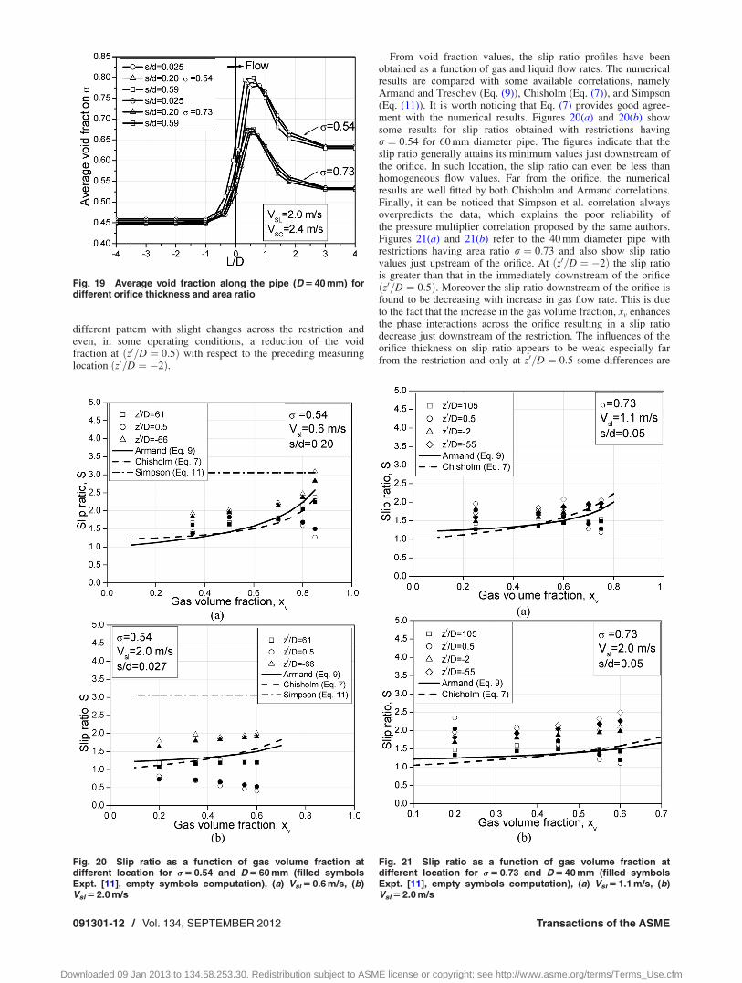
different pattern with slight changes across the restriction andeven, in some operating conditions, a reduction of the voidfraction at z0=D ¼ 0:5ð Þ with respect to the preceding measuringlocation z0=D ¼ �2ð Þ.

From void fraction values, the slip ratio profiles have beenobtained as a function of gas and liquid flow rates. The numericalresults are compared with some available correlations, namelyArmand and Treschev (Eq. (9)), Chisholm (Eq. (7)), and Simpson(Eq. (11)). It is worth noticing that Eq. (7) provides good agree-ment with the numerical results. Figures 20(a) and 20(b) showsome results for slip ratios obtained with restrictions havingr ¼ 0:54 for 60 mm diameter pipe. The figures indicate that theslip ratio generally attains its minimum values just downstream ofthe orifice. In such location, the slip ratio can even be less thanhomogeneous flow values. Far from the orifice, the numericalresults are well fitted by both Chisholm and Armand correlations.Finally, it can be noticed that Simpson et al. correlation alwaysoverpredicts the data, which explains the poor reliability ofthe pressure multiplier correlation proposed by the same authors.Figures 21(a) and 21(b) refer to the 40 mm diameter pipe withrestrictions having area ratio r ¼ 0:73 and also show slip ratiovalues just upstream of the orifice. At z0=D ¼ �2ð Þ the slip ratiois greater than that in the immediately downstream of the orificez0=D ¼ 0:5ð Þ. Moreover the slip ratio downstream of the orifice is

found to be decreasing with increase in gas flow rate. This is dueto the fact that the increase in the gas volume fraction, xv enhancesthe phase interactions across the orifice resulting in a slip ratiodecrease just downstream of the restriction. The influences of theorifice thickness on slip ratio appears to be weak especially farfrom the restriction and only at z0=D ¼ 0:5 some differences are

Fig. 19 Average void fraction along the pipe (D 5 40 mm) fordifferent orifice thickness and area ratio

Fig. 20 Slip ratio as a function of gas volume fraction atdifferent location for r 5 0.54 and D 5 60 mm (filled symbolsExpt. [11], empty symbols computation), (a) Vsl 5 0.6 m/s, (b)Vsl 5 2.0 m/s

Fig. 21 Slip ratio as a function of gas volume fraction atdifferent location for r 5 0.73 and D 5 40 mm (filled symbolsExpt. [11], empty symbols computation), (a) Vsl 5 1.1 m/s, (b)Vsl 5 2.0 m/s



observed in void fraction values and hence in slip ratio values.The slip ratio generally increases slightly with increasing the ori-fice thickness.

5 Conclusions

A mathematical model for the flow through thin and thick orifi-ces in horizontal pipes with air–water mixtures has been devel-oped by using two-phase flow model in an Eulerian scheme in thisstudy. The major observations made relating to the pressure drop,void fraction and slip ratio values in the process of flow throughorifices, can be summarized as follows:

• The contraction coefficient is found to be independent of theReynolds number for values above 5� 104. With turbulentflow through orifices the contraction coefficients for singlephase flow of water are found to be slightly higher for con-traction area ratio r ¼ 0:73 than that for r ¼ 0:54.

• In single-phase flow the contraction coefficient is found to bein good agreement with the experimental data [11] as well aswith the Chisholm [3] formula predictions. The computedpressure drop across the orifice having thickness to diameterratio, s/d¼ 0.20 is slightly less than that obtained with thes/d¼ 0.025, and s/d¼ 0.05 orifices, even though all theserestrictions can be classified as thin orifices.

• The two-phase multiplier for thin orifices (s/d¼ 0.025 to 0.2)are found to be quite well correlated by Morris equation.Thicker orifices (s/d¼ 0.59) are characterized by higher pres-sure multipliers whose values are quite well fitted by theproper Chisholm formula. Finally, the two-phase multiplierspertinent to the orifice having area ratio r ¼ 0:73 showvalues close to unity (or even lower) when the gas volumefraction is less than about 0.5. The pipe diameter has very lit-tle effect on the two-phase multiplier.

• The time average void fraction generally increases across theorifice and attains the maximum value just downstream of therestriction. The results show that the void fraction usuallyattains a maximum value at a distance of around 0.5 diame-ters from the throat. The maximum void fraction can be up totwice the value recorded far from the orifice in the upstreamdirection (in the region of fully developed flow) and the cor-responding slip ratio decreases to values less than 0.5. Thisbehavior has been observed irrespective of the orifice thick-ness for the higher values of the liquid flow rate and it ismore evident for low area ratio (r ¼ 0:54).

• The slip ratio generally attains its minimum value just down-stream of the orifice, even less than that of the homogeneousflow predictions. Far from the restriction, the numericalresults are well fitted by both Chisholm and the Armand cor-relations. It is found that the Simpson et al. correlation forboth slip ratio values as well as two-phase multiplier is notreliable.

Nomenclature

A ¼ flow area (m2)CD ¼ drag coefficientD ¼ pipe diameter (m)d ¼ orifice diameter (m)~g ¼ acceleration due to gravity (m/s2)k ¼ turbulent kinetic energy_m ¼ mass flow rate (kg/s)P ¼ pressure (Pa)

DP ¼ pressure dropRed ¼ Reynolds number corresponding to orifice diameter

S ¼ slip ratios ¼ orifice thickness (m)V ¼ velocity (m/s)

Vsg ¼ superficial gas velocity (m/s)Vsl ¼ superficial liquid velocity (m/s)

x ¼ mixture qualityxv ¼ gas volume fraction (xv¼Vsg/(VsgþVsl))z ¼ distance from inlet section (m)z0 ¼ distance from restriction (m)

Greek Symbols

a ¼ void fractione ¼ dissipation rate of turbulent kinetic energyl ¼ viscosity (kg/ms)ll ¼ laminar viscositylt ¼ turbulent viscosity

leff ¼ effective viscosityU2

lo ¼ two-phase multiplierq ¼ density (kg/m3)r ¼ area ratio (r¼ (d/D)2)

rc ¼ contraction coefficientrk ¼ turbulent Prandtl number for kre ¼ turbulent Prandtl number for e��s ¼ stress tensor~v ¼ velocity vector

Subscripts

C ¼ vena contractag ¼ gasl ¼ liquidp ¼ secondary phaseq ¼ primary phase

References[1] Idelchik, I. E., Malyavskaya, G. R., Martynenko, O. G., and Fried, E., 1994,

Handbook of Hydraulic Resistances, CRC Press, Boca Raton.[2] Simpson, H. C., Rooney, D. H., and Grattan, E., 1983, ‘‘Two-Phase Flow

Through Gate Valves and Orifice Plates,” Proceedings of the InternationalConference on Physical Modelling of Multi-Phase Flow, Coventry.

[3] Chisholm, D., 1983, Two-Phase Flow in Pipelines and Heat Exchangers, Long-man Group Ed., London.

[4] Morris, S. D., 1985, “Two Phase Pressure Drop Across Valves and OrificePlates,” Proceedings of the European Two Phase Flow Group Meeting, March-wood Engineering Laboratories, Southampton, UK.

[5] Friedel, L., 1984, “Two-Phase Pressure Drop Across Pipe Fitting,” HTFSReport No. RS41.

[6] Janssen, E., 1966, “Two-Phase Pressure Loss Across Abrupt Area Contractionsand Expansions: Steam Water at 600 to 1400 PSIA,” Proceedings of the 3rdInternational Heat Transfer Conference, Chicago, IL, Vol. 5, pp. 13–23.

[7] Lin, Z. H., 1982, “Two Phase Flow Measurement With Sharp Edge Orifices,”Int. J. Multiphase Flow, 8, pp. 683–693.

[8] Saadawi, A. A., Grattan, E., and Dempster, W. M., 1999, “Two Phase PressureLoss in Orifice Plates and Gate Valves in Large Diameter Pipes,” Proceedingsof the 2nd Symposium on Two-Phase Flow Modelling and Experimentation,G. P. Celata, P. D. Marco, R. K. Shah, eds., ETS, Pisa, Italy.

[9] Kojasoy, G., Kwame, M. P., and Chang, C. T., 1997, “Two-Phase PressureDrop in Multiple Thick and Thin Orifices Plates,” Exp. Thermal Fluid Sci., 15,pp. 347–358.

[10] Bertola, V., 2004, “The Structure of Gas–Liquid Flow in a Horizontal PipeWith Abrupt Area Contraction,” Exp. Thermal Fluid Sci., 28, pp. 505–512.

[11] Fossa, M., and Guglielmini, G., 2002, “Pressure Drop and Void Fraction Pro-files During Horizontal Flow Through Thin and Thick Orifices,” Exp. ThermalFluid Sci., 26, pp. 513–523.

[12] Fossa, M., Guglielmini, G., and Marchitto, A., 2006, “Two-Phase Flow Struc-ture Close to Orifice Contractions During Horizontal Intermittent Flows,” Int.Commun. Heat Mass Transfer, 33, pp. 698–708.

[13] Jones, O. C., and Zuber, N., 1975, “The Interrelation Between Void FractionFluctuations and Flow Patterns in Two-Phase Flow,” Int. J. Multiphase Flow,2(3), pp. 273–306.

[14] Shedd, T. A., and Newell, T. A., 2004, “Characteristics of the Liquid Film andPressure Drop in Horizontal, Annular, Two-Phase Flow Through Round,Square and Triangular Tubes,” ASME J. Fluids Eng., 126(5), pp. 807–817.

[15] Grace, H. P., and Lapple, C. E., 1951, “Discharge Coefficient of Small Diame-ter Orifices and Flow Nozzles,” Trans. ASME, 73, pp. 639–647.

[16] Bullen, P. R., Cheeseman, D. J., Hussain, L. A., and Ruffel, A. E., 1987, “TheDetermination of Pipe Contraction Coefficients for Incompressible TurbulentFlow,” Int. J. Heat Fluid Flow, 8, pp. 111–118.

[17] Benedict, R. P., 1980, Fundamentals of Pipe Flow, Wiley–Interscience, NewYork.

[18] Collier, J. G., and Thome, J. R., 1994, Convective Boiling and Condensation,Oxford University Press, New York.



http://dx.doi.org/10.1016/0301-9322(82)90071-4

http://dx.doi.org/10.1016/S0894-1777(97)00003-4

http://dx.doi.org/10.1016/j.expthermflusci.2003.07.002

http://dx.doi.org/10.1016/S0894-1777(02)00156-5

http://dx.doi.org/10.1016/S0894-1777(02)00156-5

http://dx.doi.org/10.1016/j.icheatmasstransfer.2006.02.009

http://dx.doi.org/10.1016/j.icheatmasstransfer.2006.02.009

http://dx.doi.org/10.1016/0301-9322(75)90015-4

http://dx.doi.org/10.1115/1.1792261

http://dx.doi.org/10.1016/0142-727X(87)90008-7

INSPIRON

Highlight

INSPIRON

Highlight

INSPIRON

Highlight

INSPIRON

Highlight

INSPIRON

Highlight

INSPIRON

Highlight

INSPIRON

Highlight

INSPIRON

Underline

INSPIRON

Underline

INSPIRON

Underline

INSPIRON

Underline

INSPIRON

Highlight

INSPIRON

Underline

[19] Armand, A. A., and Treschev, G., 1947, “Investigation of the Resistance DuringMovement of the Steam–Water Mixtures in Heated Boiler Pipe at High Pres-sure,” Izvestia Vses. Teplo. Inst. AERE Lib/Trans., 816(4), pp. 1–5.

[20] Drew, D. A., 1983, “Mathematical Modeling of Two-Phase Flows,” Annu. Rev.Fluid Mech., 15, pp. 261–291.

[21] Drew, D., and Lahey, R. T., Jr., 1979, “Application of General ConstitutivePrinciples to the Derivation of Multidimensional Two-Phase Flow Equations,”Int. J. Multiphase Flow, 7, pp. 243–264.

[22] Crowe, C., Sommerfeld, M., and Tsuji, Y., 1998, Multiphase Flows With Drop-lets and Particles, CRC Press, Boca Raton.

[23] Wallis, G. B., One-Dimensional Two-Phase Flow, McGraw-Hill, New York.[24] Launder, B. E., and Spalding, D. B., 1974, “The Numerical Computation of

Turbulent Flows,” Comput. Methods Appl. Mech. Eng., 3, pp. 269–289.[25] Shih, T. H., Liou, W. W., Shabbir, A., Yang, Z., and Zhu, J., 1995, “A New k-e

Eddy-Viscosity Model for High Reynolds Number Turbulent Flows,” Comput.Fluids, 24(3), pp. 227–238.

[26] Troshko, A. A., and Hassan, Y. A., 2001, “A Two-Equation TurbulenceModel of Turbulent Bubbly Flows,” Int. J. Multiphase Flow, 27, pp.1965–2000.

[27] Wolfstein, M., 1969, “The Velocity and Temperature Distribution of One-Dimensional Flow With Turbulence Augmentation and Pressure Gradient,” Int.J. Heat Mass Transfer, 12, pp. 301–318.

[28] Chen, H. C., and Patel, V. C., 1988, “Near-Wall Turbulence Models for Com-plex Flows Including Separation,” AIAA J., 26(6), pp. 641–648.

[29] Patankar, S. V., 1980, Numerical Heat Transfer and Fluid Flow, McGraw-Hill,Hemisphere, Washington, D.C.

[30] Vasquez, S. A., and Ivanov, V. A., 2000, “A Phase Coupled Method for SolvingMultiphase Problems on Unstructured Meshes,” Proceedings of the ASME Flu-ids Engineering Division Summer Meeting (FEDSM2000), FED, Boston, MA,Vol. 251, pp. 659–664.

[31] Ansari, M. R., and Shokri, V., 2007, “New Algorithm for the Numerical Simu-lation of Two-Phase Stratified Gas–Liquid Flow and Its Application for Analyz-ing the Kelvin–Helmholtz Instability Criterion With Respect to Wave LengthEffect,” Nucl. Eng. Design, 237, pp. 2302–2310.

[32] Wesseling, P., 1992, An Introduction to Multigrid Methods, Wiley, UK.[33] Weiss, J. M., Maruszewski, J. P., and Smith, W. A., 1999, “Implicit Solution of

Preconditioned Navier–Stokes Equations Using Algebraic Multigrid,” AIAA J.,37(1), pp. 29–36.



http://dx.doi.org/10.1146/annurev.fl.15.010183.001401

http://dx.doi.org/10.1146/annurev.fl.15.010183.001401

http://dx.doi.org/10.1016/0301-9322(79)90024-7

http://dx.doi.org/10.1016/0045-7825(74)90029-2

http://dx.doi.org/10.1016/0045-7930(94)00032-T

http://dx.doi.org/10.1016/0045-7930(94)00032-T

http://dx.doi.org/10.1016/S0301-9322(01)00043-X

http://dx.doi.org/10.1016/0017-9310(69)90012-X

http://dx.doi.org/10.1016/0017-9310(69)90012-X

http://dx.doi.org/10.2514/3.9948

http://dx.doi.org/10.1016/j.nucengdes.2007.04.005

http://dx.doi.org/10.2514/2.689

INSPIRON

Highlight

INSPIRON

Highlight

INSPIRON

Highlight

INSPIRON

Underline

INSPIRON

Underline

INSPIRON

Underline

INSPIRON

Underline

Documents

Single-Phase and Two-Phase Flow Through Orifices in Horizontal PipesThin and Thick