Simulation of Supercritical Fluid Extraction Process Using COMSOL

Multiphysics

Priyanka*1, Shabina. Khanam

2

1Priyanka. Indian Institute of Technology Roorkee, Roorkee

2Shabina Khanam. Indian Institute of Technology Roorkee, Roorkee

*Corresponding author: Department of Chemical Engineering, Indian Institute of Technology Roorkee, Roorkee

Haridwar, Uttarakhand 247667, priyankakatiyar65@gmail.com

Abstract: The present work deals with the simulation

of mathematical model for supercritical extraction

process of Sage leaves . Reverchon,1996 extracted

sage oil using supercritical extraction method from

sage leaves at 9 MPa and 50 ᵒC. Different hypotheses

were tested on vegetable matter geometry, and their

incidence on the model performance was evaluated.

The model was also developed by Reverchon, 1996.

Four mean size of sage leaves ranging from 0.25 to

3.10 mm were taken for extraction with other

experimental conditions and process parameters.

Experimental results were fitted in the model and the

results obtained were in a good agreement. In present

work, same mathematical model is solved using

COMSOL multiphysics and results are compared

with the results given in literature to find the

utilisation of COMSOL multiphysics.

Keywords: Supercritical fluid extraction, Sage

leaves, Equation based modeling

1. Introduction

Supercritical extraction process is promising and

benign alternative to extract high value added

products for the food, cosmetics, and pharmaceutical

industries. The fluid above this critical temperature

and pressure is called a supercritical fluid.

Supercritical fluid extraction is a technique that

exploits the solvent power of supercritical fluids at

temperatures and pressures near the critical point.

With supercritical fluid extraction (SFE) higher

yields and better quality products can be achieved.

Carbon di-oxide at its supercritical conditions (SC-

CO2), is the most desirable solvent for the extraction

of natural products as it is non-toxic, inexpensive,

non-flammable, and non-polluting. SC-CO2 is used in

food applications as a solvent for the extraction of

non-polar solutes. Supercritical extraction method is

used for the extraction of several natural products

such as: sunflower seed, watermelon seed, black

pepper seed, rosemary flower, ginger root, turmeric

root etc.

2. Literature Review

Several mathematical models on supercritical fluid

extraction process have been proposed by different

authors as given in literature. Reverchon, 1996 used

sage leaves for the extraction of sage oil using

supercritical extraction method at 9 MPa and 50 ᵒC.

The mean particle size was evaluated by mechanical

sieving. Batches of 3.10, 0.75, 0.50 and 0.25 mm

mean particle sizes were used for the extraction. A

mathematical model based on differential mass

balances performed along the extraction bed was also

developed by Reverchon, 1996 and used to fit

experimental data of sage leaves. Other experimental

conditions and process parameters used for the

extraction are shown in table 1.

Table-1 Experimental conditions and process

parameters

Parameter Value

Flow rate (Q) 8.83 g/min

Porosity (ε) 0.4

Superficial viscosity 0.455*10-3

m/s

Fluid phase coefficient (kf) 1.91*10-5

m/s

Amount of seed (W) 0.160 kg

Volumetric partition coefficient

(kp)

0.2

Diffusivity (Di) 6.0*10-13

m2/s

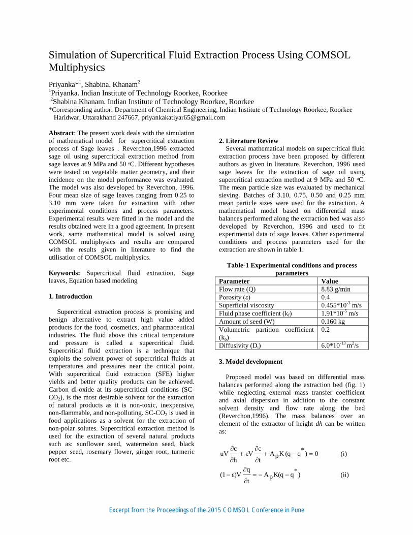
3. Model development

Proposed model was based on differential mass

balances performed along the extraction bed (fig. 1)

while neglecting external mass transfer coefficient

and axial dispersion in addition to the constant

solvent density and flow rate along the bed

(Reverchon,1996). The mass balances over an

element of the extractor of height dh can be written

as:

0)*

q(qKpAt

cεV

h

cuV

(i)

)*

qK(qpAt

qε)V(1

(ii)

Excerpt from the Proceedings of the 2015 COMSOL Conference in Pune

With initial and boundary condition as:

0hat0t)c(0,

0tat0qq0,c

(iii)

A linear relationship was used due to lack of

experimental data:

*.qpkc (iv)

In equation (ii), Vε1

KpA

depends on the geometry of

particles and dimensionally equal to the 1/s, thus::

i

D

2l

μVε1

KpA

it

(v)

For spherical particle µ is equal to 3/5 and l is equal

to Vp/Ap (particle volume/particle surface).

Figure 1: Schematic representation of extraction bed

Authors solved the model by rewriting mass balance

equations as a set of 2n equations as given in eq. (vi)

and (vii) and solved numerically using fourth order

Rungee - Kutta method.

0dt

ndq

n

Vε)(1

dt

ndc

n

Vε)1ncn(c

ρ

W (vi)

)*nqn(q

it

1

dt

ndq (vii)

4. Model solved by using COMSOL multiphysics

The model proposed by Reverchon, 1996, as

explained above, is solved using COMSOL

multiphysics 5.0 software in the present work.

Equation based modeling approach is used to solve

the model equations instead of any built-in physics

interface like Chemical Spices Transport Physics

Interface. It is recommended to use built-in physics

interfaces to enable ready-made post-processing

variables and other tools for faster model setup with

much lower risk of human error. To solve the model

equations (i) and (ii), two interfaces were taken under

Mathematics branch: (i) PDE interfaces and (2) ODE

and DAE interfaces. For equation (i), The

Coefficient form PDE interface is taken because it

contains two independent variable 't 'and 'h' and

Domain ODEs and DAEs is used for equation (ii)

because of presence single independent variable 't'.

For the solution, 1D geometry is taken to simplify the

problem. Time dependent study option is taken after

choosing two different interfaces under Mathematics

branch.

5. Use of COMSOL multiphysics

Model equations are solved considering 1D

geometry under Model wizard window on COMSOL

desktop. Under Select Physics option, Mathematics

interface group is selected and then Coefficient form

PDE under PDE subgroup and global ODEs and

DAEs interface under ODE and DAE subgroup are

added. After adding physics, Time dependent study

was carried out as both models equations are

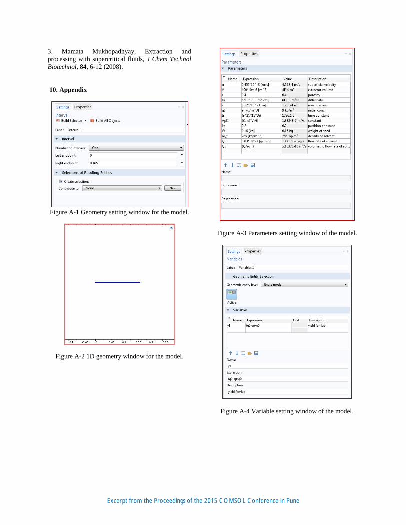
differentiated with respect to time 't'. While entering

Interval values (Left endpoint and Right endpoint)

under Geometry option in Model builder window and

a line is formed as 1D geometry as shown in Fig. A-1

and A-2. Some parameters used in the process are

constant and their values are added in parameters

section in Model builder window as given in Fig. A-

3. Two dependent variable (solvent phase oil

concentration 'c' and solid phase oil concentration 'q')

and two independent variables (time 't' and height of

bed 'h') are considered for solving the equations.

Other than these variables, a variable is added by

right clicking the Definitions option under

Component 1 section in Model builder window and

Z=h

Super critical fluid and

extracted solute

Z=0

Δh

C0=0; u0

Cz

Cz+Δz

Super critical fluid

Excerpt from the Proceedings of the 2015 COMSOL Conference in Pune

can be seen in Fig. A-4. Further, Equation (1) is

compared with the default equation of Coefficient

form PDE and values of coefficients are added in the

Coefficient form PDE 1 window as shown in Fig. A-

5. Initial value is added with help of pointwise

constraint setting because as given in eq. (iii), value

of dependent variable 'c' is zero at h=0 and can be

noticed through Fig. A-6 and A-7. For applying

pointwise constraint setting Left endpoint is

considered as h=0 (after which extraction starts) and

Right endpoint is considered as Z= h, height of

column (extraction ends) as given in figure 1.

Similarly eq. (ii) is compared with the default

equation given in Distributed ODE 1 interface and

value of coefficients are added as shown in Fig. A-8.

Initial conditions are added for this equation as given

in eq. (iii) in Initial values section under Domain

ODEs and DAEs interface and can be seen by Fig. A-

9. This study is time dependent study so a range for

time value should also be given for the solution of

equations and is shown in Fig. A-10. Under study

setting, time unit, time range and tolerance values are

added and then model is computed to get the results

as shown in Fig. A-11.

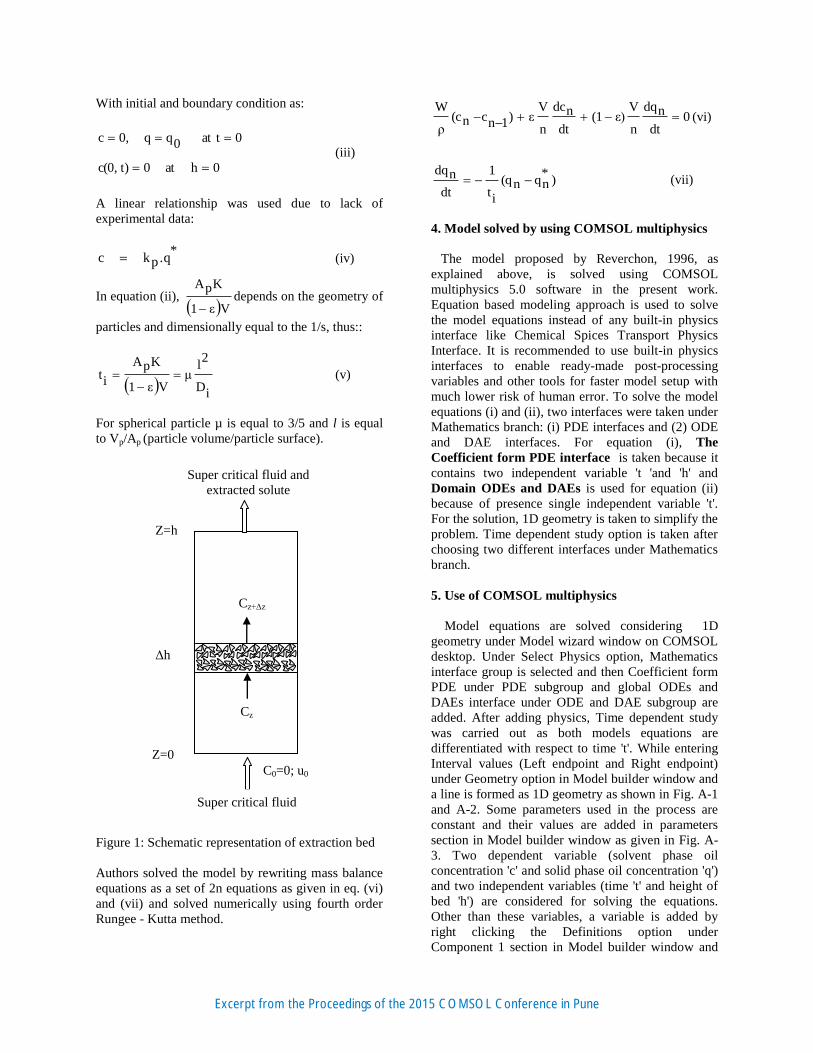
6. Results and Discussions

Results by the computation of the model are

compared with the results given in the literature.

Results are computed considering four different

particle size and plotted between extraction yield

(amount of oil extracted*100/amount of oil available

in seed) and extraction time. As given in literature,

Extraction yield values for 0.25 and 0.5 mm particle

size are 100% as can be seen from Fig. 2 and shows

that almost total amount of oil available are extracted

by the extraction process. A lesser extraction yield

value is observed for 0.75 and 3.1 mm particle, which

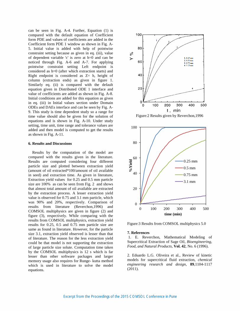
was 90% and 20%, respectively. Comparison of

results from literature (Reverchon,1996) and

COMSOL multiphysics are given in figure (2) and

figure (3), respectively. While comparing with the

results from COMSOL multiphysics, extraction yield

results for 0.25, 0.5 and 0.75 mm particle size are

same as found in literature. However, for the particle

size 3.1, extraction yield observed is lesser than that

of literature. The reason for the less extraction yield

could be that model is not supporting the extraction

of large particle size solute. Computation time taken

by the COMSOL multiphysics is 12 s which is far

lesser than other software packages and larger

memory usage also requires for Runge- kutta method

which is used in literature to solve the model

equations.

Figure:2 Results given by Reverchon,1996

Figure:3 Results from COMSOL multiphysics 5.0

7. References

1. E. Reverchon, Mathematical Modeling of

Supercritical Extraction of Sage Oil, Bioengineering,

Food, and Natural Products, Vol. 42, No. 6 (1996).

2. Eduardo L.G. Oliveira et al., Review of kinetic

models for supercritical fluid extraction, chemical

engineering research and design, 89,1104-1117

(2011).

0

20

40

60

80

100

0 100 200 300 400 500

%Y

ield

time (min)

0.25 mm

0.5 mm

0.75 mm

3.1 mm

Excerpt from the Proceedings of the 2015 COMSOL Conference in Pune

3. Mamata Mukhopadhyay, Extraction and

processing with supercritical fluids, J Chem Technol

Biotechnol, 84, 6-12 (2008).

10. Appendix

Figure A-1 Geometry setting window for the model.

Figure A-2 1D geometry window for the model.

Figure A-3 Parameters setting window of the model.

Figure A-4 Variable setting window of the model.

Excerpt from the Proceedings of the 2015 COMSOL Conference in Pune

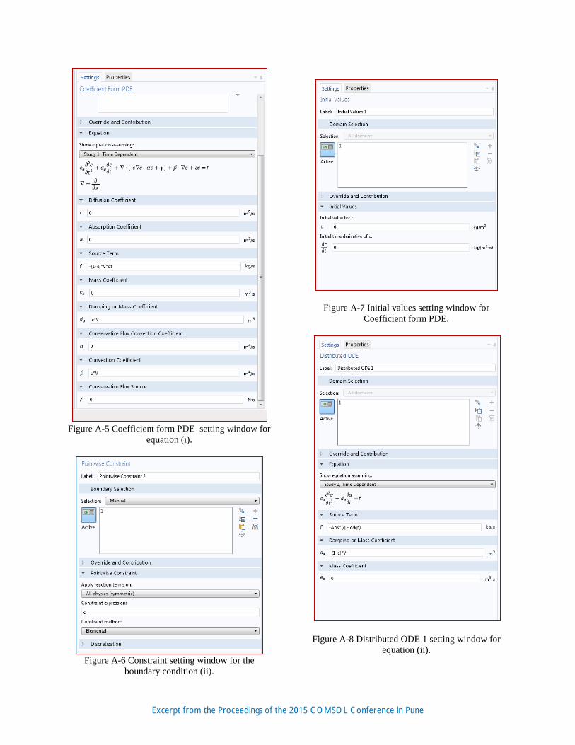
Figure A-5 Coefficient form PDE setting window for

equation (i).

Figure A-6 Constraint setting window for the

boundary condition (ii).

Figure A-7 Initial values setting window for

Coefficient form PDE.

Figure A-8 Distributed ODE 1 setting window for

equation (ii).

Excerpt from the Proceedings of the 2015 COMSOL Conference in Pune

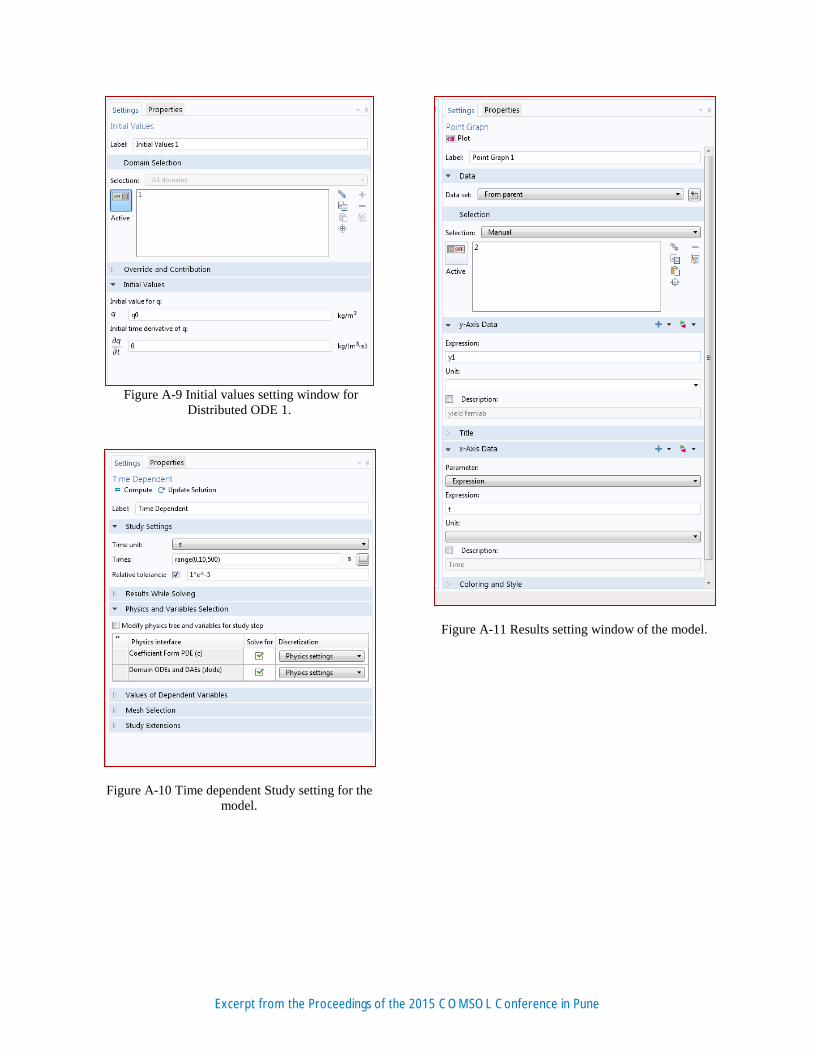
Figure A-9 Initial values setting window for

Distributed ODE 1.

Figure A-10 Time dependent Study setting for the

model.

Figure A-11 Results setting window of the model.

Excerpt from the Proceedings of the 2015 COMSOL Conference in Pune