Embed Size (px)
Citation preview

Department of Science and Technology Institutionen för teknik och naturvetenskap Linköping University Linköpings universitet
gnipökrroN 47 106 nedewS ,gnipökrroN 47 106-ES
LiU-ITN-TEK-A--11/060--SE
Simulation and Optimization ofFrequency Reuse in OFDMA
NetworksAzeem Waqar
Muhammad Ammar Zafar
2011-09-19

LiU-ITN-TEK-A--11/060--SE
Simulation and Optimization ofFrequency Reuse in OFDMA
NetworksExamensarbete utfört i elektroteknik
vid Tekniska högskolan vidLinköpings universitet
Azeem WaqarMuhammad Ammar Zafar
Examinator Di Yuan
Norrköping 2011-09-19

Upphovsrätt
Detta dokument hålls tillgängligt på Internet – eller dess framtida ersättare –under en längre tid från publiceringsdatum under förutsättning att inga extra-ordinära omständigheter uppstår.
Tillgång till dokumentet innebär tillstånd för var och en att läsa, ladda ner,skriva ut enstaka kopior för enskilt bruk och att använda det oförändrat förickekommersiell forskning och för undervisning. Överföring av upphovsrättenvid en senare tidpunkt kan inte upphäva detta tillstånd. All annan användning avdokumentet kräver upphovsmannens medgivande. För att garantera äktheten,säkerheten och tillgängligheten finns det lösningar av teknisk och administrativart.
Upphovsmannens ideella rätt innefattar rätt att bli nämnd som upphovsman iden omfattning som god sed kräver vid användning av dokumentet på ovanbeskrivna sätt samt skydd mot att dokumentet ändras eller presenteras i sådanform eller i sådant sammanhang som är kränkande för upphovsmannens litteräraeller konstnärliga anseende eller egenart.
För ytterligare information om Linköping University Electronic Press seförlagets hemsida http://www.ep.liu.se/
Copyright
The publishers will keep this document online on the Internet - or its possiblereplacement - for a considerable time from the date of publication barringexceptional circumstances.
The online availability of the document implies a permanent permission foranyone to read, to download, to print out single copies for your own use and touse it unchanged for any non-commercial research and educational purpose.Subsequent transfers of copyright cannot revoke this permission. All other usesof the document are conditional on the consent of the copyright owner. Thepublisher has taken technical and administrative measures to assure authenticity,security and accessibility.
According to intellectual property law the author has the right to bementioned when his/her work is accessed as described above and to be protectedagainst infringement.
For additional information about the Linköping University Electronic Pressand its procedures for publication and for assurance of document integrity,please refer to its WWW home page: http://www.ep.liu.se/
© Azeem Waqar, Muhammad Ammar Zafar

i
Abstract
Efficient radio resource management is an important aspect when it comes to
achieving high bit rates in technologies such as the 3GPP Long Term Evolution
(LTE). This thesis aims at understanding existing frequency reuse schemes in
OFDMA networks, and to develop an algorithm for frequency allocation for irregular
cellular layouts. Previous work done in this field mostly covers schemes for regular
cells, whereas in real life cellular layouts are mostly irregular. A comparison of the
existing allocation schemes for the users near the boundary of the cells, also known as
edge users, with our scheme is presented.
Reuse-1, Fractional frequency reuse-3 with random frequency allocation (FFR3-RFA)
(for edge users) and our algorithmic frequency allocation (FFR3-AFA) scheme are
simulated and compared. FFR3-AFA algorithm assigns a frequency sub-band to a cell
by considering the frequency allocations in the neighbor cell edges and the overlap
area between those neighboring cells. Static simulations were performed with one
user per base station and constant downlink traffic of 100 Kbits/sec, so that all the
resources are utilized and there is maximum interference. This way, the difference
between the frequency reuse schemes is much more evident. The throughput for our
calculation is the ratio of the total successful packets sent in the network and the total
packets sent in the network. Small scenarios are considered with different downlink
data rates and the results show that FFR3-AFA has better performance than the other
two techniques. There is also room for improvement in the algorithm by introducing
other factors into the equation other than overlap area, such as user throughput.

ii

iii
Acknowledgements
We would like to thank our supervisor Prof. Di Yuan for his support and guidance
throughout the thesis work. His provided us with all the guidelines and gave us a
clear picture on what to aim for this thesis work.
Also, we would like to thank Lei Chen who guided us from time to time during our
work technically and helped us in choosing the software platform for the thesis
work.
Lastly, we would like this opportunity to thank all our colleagues from our Masters
program and all our teachers who taught us and who helped us in one way or the
other throughout our Masters degree at Linköping University. Their technical and
motivational support always pushed us and kept us on our toes.
Regards,
Muhammad Ammar Zafar
Azeem Waqar

iv

v
Table of Contents
Chapter 1 Introduction .............................................................................................................. 1
1.1 Problem Statement ..................................................................................................... 1
1.2 Thesis Outline ............................................................................................................ 2
Chapter 2 Technical Background .............................................................................................. 3
2.1 Single Carrier Modulation .......................................................................................... 3
2.2 Frequency Division Multiplexing (FDM) .................................................................. 3
2.3 Orthogonal Frequency Division Multiplexing (OFDM) ............................................ 4
2.4 Orthogonal Frequency Division Multiple Access (OFDMA) .................................... 6
2.5 The Concept of Frequency Reuse .............................................................................. 6
2.5.1 FFR and SFR .......................................................................................................... 7
Chapter 3 Inter-Cell Interference Mitigation Techniques ......................................................... 8
3.1 Interference Mitigation .............................................................................................. 8
3.2 Proposals by Telecommunication Companies............................................................ 8
3.2.1 Ericsson’s Proposal ................................................................................................ 8
3.2.2 Nokia Siemens Networks’ (NSN) Proposal ........................................................... 9
3.2.3 Alcatel’s Proposal .................................................................................................. 9
3.2.4 Samsung’s Proposal ..............................................................................................11
Chapter 4 Literature Study ...................................................................................................... 13
Chapter 5 Simulation Platform ............................................................................................... 16
5.1 Choice of Simulation Tool ....................................................................................... 16
5.2 Open Wireless Network Simulator (OpenWNS) ..................................................... 17
5.2.1 Event Scheduler .................................................................................................. 17
5.2.2 Configurations .................................................................................................... 18
5.2.3 Evaluation ........................................................................................................... 18
5.2.4 Simulation Modules ............................................................................................ 19
Chapter 6 Optimization of FFR for Irregular Cellular Structure ............................................ 24
6.1 Frequency Reuse Schemes ....................................................................................... 24
6.1.1 Frequency Reuse-1 ............................................................................................. 24
6.1.2 FFR-3 with Random Allocation .......................................................................... 24
6.1.3 FFR-3 with Algorithmic Allocation .................................................................... 25
Chapter 7 Simulation Setup and Results ................................................................................. 32
7.1 Simulation Model and Parameters ........................................................................... 32
7.2 Choosing Cell Edge .................................................................................................. 35

7.3 Analysis of Results ................................................................................................... 36
7.4 Scenarios .................................................................................................................. 38
Chapter 8 Conclusions and Future Work ................................................................................ 42
8.1 The Algorithm .......................................................................................................... 42
8.2 Choosing a Tool........................................................................................................ 42
8.3 The Scenario ............................................................................................................. 42
8.4 Effect of User Placements ........................................................................................ 42
8.5 Results ...................................................................................................................... 43
8.6 Future Work .............................................................................................................. 43
Bibliography ........................................................................................................................... 44

vii
List of Abbreviations
ARMA Autoregressive Moving Average
ASK Amplitude Shift Keying
ATM Asynchronous Transfer Mode
BS Base Station
CBR Constant Bit Rate
CCU Cell Centre User
CEU Cell Edge User
CP Cyclic Prefix
DFT Discrete Fourier Transform
DSA Dynamic Sub-carrier Allocation
FDM Frequency Division Multiplexing
FDMA Frequency Division Multiple Access
FFR Fractional Frequency Reuse
FFT Fast Fourier Transform
FSK Frequency Shift Keying
GSM Global System for Mobile Communications
ICI Inter-cell interference
IDFT Inverse Discrete Fourier Transform
IFFT Inverse Fast Fourier Transform
IP Internet Protocol
ISI Inter-symbol Interference
LOS Line of Sight
MMPP Markov-Modulated Poisson Process
NLOS Non-Line of Sight
NSN Nokia Siemens Networks
OFDM Orthogonal Frequency Division Multiplexing
OFDMA Orthogonal Frequency Division Multiple Access
OpenWNS Open Wireless Networks Simulator

viii
PP Point Process
PSK Phase Shift Keying
QoS Quality of Service
RISE Radio Interference Simulation Engine
RNC Radio Network Controller
SFR Soft Frequency Reuse
SINR Signal to Interference Noise Ratio
TCP Transmission Control Protocol
TDMA Time Division Multiple Access
UDP User Datagram Protocol
VOIP Voice over Internet Protocol
Wi-Fi IEEE 802.11 standard
WiMAC WiMAX Medium Access Control
WiMAX Worldwide Interoperability for Microwave Access

1
Chapter 1
Introduction
With the emergence of mobile technologies in the early 1980's no one could have thought
that within half a century cellular phones will become such an integral part of our lives. As
the technology progressed, so did the demands of the users and the technology had to come
out of its shell, of just providing quality voice service, to providing non-traditional services
like real-time video and data services. This puts more stress on the radio resources which
were always limited. From GSM to 3G and OFDMA systems, the focus has always been on
effectively utilizing the frequency spectrum.
The access network in mobile networks is based on the cellular approach because of the
limitation on frequency resources. To improve the spectrum efficiency frequency reuse is
implemented in these cellular systems. For CDMA systems, frequency reuse factor is equal
to 1 i.e. all frequency resources are available in each cell. However, in OFDMA networks, if
frequency reuse factor of 1 is used, co-channel interference (CCI) would be introduced
because of same resources being simultaneously occupied by different users in adjacent cells,
specifically for those users which reside close to the cell boundary. This interference will
cause degradation in system performance and service quality for edge users.
To reduce the CCI one technique could be to implement a reuse factor greater than 1 but it
reduces the spectrum efficiency and is thus not feasible for OFDMA networks. Several
techniques have been developed to overcome this interference problem. The technique that is
investigated in this thesis is Fractional Frequency Reuse (FFR). The main idea behind FFR is
to logically divide the cell into inner and outer regions and use reuse factor of 1 for the inner
region and an increased reuse factor for outer regions. This has the effect of users close to
cell boundaries experiencing reduced interference from the adjacent cells and having
improved service quality.
1.1 Problem Statement
Related studies on FFR deals with standard hexagonal shaped cell layouts which may be
good for theoretical measurements but are far from the cellular layouts used in real network
scenarios. Real-life networks have a very irregular cellular layout with high variations in
signal propagation, and optimization is required continuously to improve the overall
performance of the network. Most of the previous studies of FFR do not provide an optimal

2
solution for real life networks because of irregularity in cell patterns. FFR solutions need to
be optimized to enhance the cell edge performance for such irregular networks.
The task of this thesis is to simulate fractional frequency reuse in OFDMA systems and to
develop an optimization algorithm to optimize the fractional frequency reuse for realistic
cellular layout. The simulation aims at comparing the optimized FFR-3 scheme (FFR3-AFA)
with randomly allocated FFR-3 scheme (FFR3-RFA) and the classical reuse-1 scheme for
realistic layout of OFDMA cellular networks. The work in a nut-shell consists of selection of
the simulation platform, development of simulation scenarios, programming in the selected
simulation environment as well as performance evaluation and analysis.
1.2 Thesis Outline
A theoretical background is given in Chapter 2 which goes step by step from single carrier
modulation to OFDMA. The concept of frequency reuse is also briefly discussed. This
chapter assumes a general understanding of basic modulation techniques and signal
processing.
Chapter 3 covers inter-cell interference (ICI) mitigation techniques proposed by major
telecommunication vendors. The text explains their proposals briefly.
A brief description of related work on frequency allocation schemes for OFDMA networks is
presented in Chapter 4.
An overview of the simulation tool used for simulations is described in Chapter 5. It covers
the structural organization and simulation modules of the simulator.
Chapter 6 presents a detailed description of the frequency allocation techniques implemented
in the thesis. It also presents the algorithm used to optimize the cell edge performance.
Simulation scenarios and results are presented in Chapter 7, followed by conclusions and
possible continuation of work in Chapter 8.

3
Chapter 2
Technical Background
2.1 Single Carrier Modulation
In single carrier modulation, information signal is modulated on a single carrier using either
phase, amplitude or the frequency parameter of the carrier. These techniques are called phase
shift keying (PSK), amplitude shift keying (ASK) and frequency shift keying (FSK)
respectively. As we move to higher bandwidths in single carrier systems, the symbol/bit
duration decreases significantly, thus making the modulated signals more prone to noise,
interference and other impairments. The end result is loss of information as the receiver is
unable to recover the transmitted information.
2.2 Frequency Division Multiplexing (FDM)
Frequency Division Multiplexing (FDM) is a multi-carrier transmission scheme and is an
extension to the single carrier modulated systems. It uses multiple sub-carriers for the same
channel i.e. the spectrum (available bandwidth) is divided into different sub-channels and
several data streams can be concurrently transmitted over the channel. The individual data
rates of each sub-channel taken together gives the overall data rate of the system. One
important point to note is that the data which is to be divided into these sub-channels may not
be from the same source. Hence, different users can be served simultaneously over the same
channel using different sub-channels.
By breaking the bandwidth into small sub-channels, the frequency response of each sub-
channel can be considered flat. This flat response helps to simplify the equalizer design and
lowers the complexity of the receiver [1]. Different data streams can be transmitted
simultaneously without interfering with each other.
If we consider the frequency spectrum of FDM, the main lobes of the sub-channels do not
overlap, as shown in Fig. 2.1. In fact, the two sub-carriers are separated by a guard band for
minimum interference. These guard bands ease the demands on the cut-off frequencies of the
filters in the receiver, and also protect against frequency inaccuracies. Disadvantage of these
guard bands is that it lowers the system’s spectrum efficiency and effective information rate
as compared to a single carrier system with similar modulation.

4
Figure 2.1 FDM sub-carriers.
.
The main advantage of FDM over single carrier modulation is the ability to overcome
narrowband interference. Since the interference is frequency dependent, only one of the sub-
bands will be affected. Additional immunity against impulse noise and frequency reflections
is achieved because each sub-carrier has a lower data rate and hence the data symbol period
will be longer. Also, we can have separate modulation and demodulation techniques for
different data streams (sub-channels).
2.3 Orthogonal Frequency Division Multiplexing (OFDM)
Orthogonal Frequency Division Multiplexing (OFDM) is also a multi-carrier modulation
technique and is based on the division of available bandwidth into multiple sub-channels.
OFDM emphasizes that FDM’s bandwidth usability can be made much more efficient by
allowing overlap between the main lobes of the sub-channels. This is possible by making the
overlap in a clever way i.e. using sub-carriers that are orthogonal to each other. By
introducing this orthogonality property to the sub-carriers, guard bands that were required for
FDM system would no longer be needed. The resulting OFDM signal spectrum is shown in
Fig. 2.2.

5
Figure 2.2 OFDM signal with 6 sub-carriers.
If we denote φ (t) as sub-carriers, then in time domain we can write the equation for each
sub-carrier as
)2sin()2cos(1
)(2
tfjtfeT
t ii
tfj
ii ππφ π +== (2.1)
Here the subscript i is for individual sub-carriers and fi is the centre frequency of a particular
sub-carrier. The centre frequency of a particular sub-carrier is given as
fmff oi ∆⋅+=
(2.2)
Here fo is the base frequency and m is the sub-carrier number and ∆f is the sub-carrier
spacing.
The orthogonality property which the sub-carriers hold in OFDMA is given as
nm
nmdttLtL mn
=
≠
=∫∞
01
0)()( (2.3)
Here Ln (t) and Lm (t) are the two sub-carriers, and m and n are the sub-carrier numbers.
OFDM allows only one user on the channel at any given time. To provide support for
multiple users, a multiple access scheme is required with OFDM. TDMA or FDMA could be
used but neither of these techniques is time or frequency efficient. A more efficient technique
that could be useful for OFDM is Orthogonal Frequency Division Multiple Access
(OFDMA).
6
2.4 Orthogonal Frequency Division Multiple Access (OFDMA)
OFDMA can be thought of a multi-user OFDM which allows multiple users to access the
channel at the same time. In OFDMA, sub-carriers are distributed among different users for
intervals of time so that they can transmit and receive within their own channel without
experiencing any significant interference from users on other sub-carriers. Each single user
can be assigned one or multiple sub-carriers depending on the requested data rate.
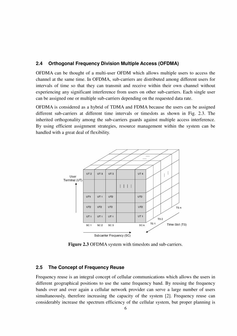
OFDMA is considered as a hybrid of TDMA and FDMA because the users can be assigned
different sub-carriers at different time intervals or timeslots as shown in Fig. 2.3. The
inherited orthogonality among the sub-carriers guards against multiple access interference.
By using efficient assignment strategies, resource management within the system can be
handled with a great deal of flexibility.
Figure 2.3 OFDMA system with timeslots and sub-carriers.
2.5 The Concept of Frequency Reuse
Frequency reuse is an integral concept of cellular communications which allows the users in
different geographical positions to use the same frequency band. By reusing the frequency
bands over and over again a cellular network provider can serve a large number of users
simultaneously, therefore increasing the capacity of the system [2]. Frequency reuse can
considerably increase the spectrum efficiency of the cellular system, but proper planning is

7
required to overcome the interference caused by the common use of the same frequency
bands. Because of the closeness of frequency bands, interferences such as adjacent channel
interference and co-channel interference can severely degrade the quality of service provided
to a mobile user. Efficient frequency allocation techniques have been developed over the
years to minimize these interferences and maximize the benefits of frequency reuse. For
OFDMA systems, techniques such as FFR and SFR are popular choices.
2.5.1 FFR and SFR
FFR and Soft Frequency Reuse (SFR) are two well-known interference mitigation techniques
in OFDMA networks. In both these allocation schemes, the cell is logically divided into inner
and outer regions and similarly the users are differentiated as cell-centre users and cell edge
users. Both allocation techniques apply reuse factor of one to cell centre. However, cell edge
users are served with a reuse factor greater than one with slight difference between the two
techniques. In FFR, the given bandwidth is split into two parts, inner and outer. The inner
part is allocated to each base station i.e. fully reused by all base stations. The outer part is
further divided among base stations with a frequency reuse greater than one trying to
maintain that adjacent cells are allocated a different sub-band from the outer part. In SFR, the
overall bandwidth is shared by all base stations, but a power bound on certain sub-bands is
introduced such that some sub-bands are transmitted with higher power in one cell and some
sub-bands in other [3].
.
8
Chapter 3
Inter-Cell Interference Mitigation Techniques
3.1 Interference Mitigation
The cellular concept in mobile communications is faced with issues from inter-cell
interference (ICI). This interference arises because of the duplication of signals/resources in
the neighboring cells, and has the effect of degrading the service quality of the users. If each
base station in the system uses the entire bandwidth resources simultaneously, any mobile
station which is close to the boundary of a cell would suffer from interference created by the
same resource in the adjacent cell. This interference degrades the QoS of the mobile station
located at the cell edge. Users close to the base station, also called Cell Centre Users (CCU),
may not be severely affected by this interference because of their distance from the
neighboring base stations. At cell edges, because the cells do not have a definite boundary,
the frequencies come across each other more which has drastic effects on the cell edge users.
The cellular concept becomes realistic only if efficient solutions can be provided for ICI.
Otherwise, there will be large areas within the coverage area of a telecommunication operator
where the users cannot be served properly and the concept of efficient resource management
is ruined. One solution to this issue is the allocation of alternate resources to cells, i.e.
adjacent cells are allocated totally different frequencies such that there is no interference.
Ever increasing demand of data services requires the need for increasing data rates and using
such schemes is not a solution anymore. Interference mitigation techniques that can maintain
a frequency reuse close to 1 (entire bandwidth available to each cell) need to be worked out.
3.2 Proposals by Telecommunication Companies
3.2.1 Ericsson’s Proposal
In the allocation scheme proposed by Ericsson only a portion of total resources is made
available for allocation to cell edge users with full power, while cell centre users use the
whole spectrum with restricted power. The sub-bands used for cell edges are orthogonal
between neighboring cells to reduce interference. The cost is reduced bandwidth for cell edge
users [4]. An example is shown in Fig. 3.1.

9
Figure 3.1 Ericsson’s proposed scheme with orthogonal cell edge sub-bands F1, F2, and F3 in
neighboring cells.
3.2.2 Nokia Siemens Networks’ (NSN) Proposal
Nokia Siemens Networks proposed a Soft Frequency Reuse (SFR) technique. It uses a static
power profile in each cell. The transmit power is kept constant for a set of sub-carriers, called
‘frequency resource units’ by NSN. When allocating different sets of sub-carriers to cells,
coordination is required such that frequency resource units with higher power in a cell
coexist with relatively lower power resource units in the neighboring cells [5]. This
assignment of static power profiles to cells reduces the inter-cell interference at cell edges.
3.2.3 Alcatel’s Proposal
Alcatel proposed two strategies for inter-cell interference mitigation:
• Interference coordination strategy 1 (network power planning)
• Interference coordination strategy 2 (on demand basis)

10
In the first method, the frequency spectrum is divided into several subsets. Suppose S is the
total number of subsets. The value of S is proposed to be 7 or 9. Each subset is referred by Fn,
where n is from 1 to S. Networking planning is done in such a way that always a different
frequency subset Fn has reduced power in each sector. So in sector Cn the power of the subset
Fn is limited to the cell centre. For example, if a user U1 (in C6) approaches sector C1, as
shown in Fig. 3.2, it gets frequency allocation from frequency subset F1 as F1 is used with
reduced power in C1. So all users approaching C1 from the outside are allocated subset F1 by
their respective base stations as long as they remain in the cell edges of their respective cells
and before a handover to cell C1 has taken place. For details on the network power planning
scheme the readers are referred to [6].
Figure 3.2 Interference coordination strategy 1.
The second interference coordination strategy is a dynamic technique and does not require
network planning to deal with cell edge users or users which are approaching the cell
boundary. When a user approaches the cell boundary between two cells, it will experience
interference from other cells. The user reports this interference to its serving base station. The
serving base station coordinates with its neighboring (interfering) base station and a power
restriction is placed on a set of frequency bands in the neighbor and those bands are granted
to the serving base station. Thus, a resource is restricted in the neighbor and is assigned to the
serving station [6]. The result is improved service for the cell edge users. The method is
shown in Fig. 3.3.
11
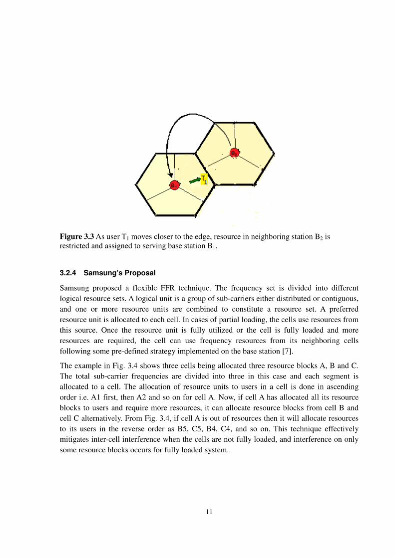
Figure 3.3 As user T1 moves closer to the edge, resource in neighboring station B2 is
restricted and assigned to serving base station B1.
3.2.4 Samsung’s Proposal
Samsung proposed a flexible FFR technique. The frequency set is divided into different
logical resource sets. A logical unit is a group of sub-carriers either distributed or contiguous,
and one or more resource units are combined to constitute a resource set. A preferred
resource unit is allocated to each cell. In cases of partial loading, the cells use resources from
this source. Once the resource unit is fully utilized or the cell is fully loaded and more
resources are required, the cell can use frequency resources from its neighboring cells
following some pre-defined strategy implemented on the base station [7].
The example in Fig. 3.4 shows three cells being allocated three resource blocks A, B and C.
The total sub-carrier frequencies are divided into three in this case and each segment is
allocated to a cell. The allocation of resource units to users in a cell is done in ascending
order i.e. A1 first, then A2 and so on for cell A. Now, if cell A has allocated all its resource
blocks to users and require more resources, it can allocate resource blocks from cell B and
cell C alternatively. From Fig. 3.4, if cell A is out of resources then it will allocate resources
to its users in the reverse order as B5, C5, B4, C4, and so on. This technique effectively
mitigates inter-cell interference when the cells are not fully loaded, and interference on only
some resource blocks occurs for fully loaded system.

12
Cell-A
A1
A2
A3
A4
A5
B1
B2
B3
B4
B5
C1
C2
C3
C4
C5
Cell-B
Cell-CB
, C
A,
CA
, B
AB
C
Figure 3.4 Flexible FFR proposed by Samsung.
13
Chapter 4
Literature Study
Design and development of efficient resource/frequency allocation techniques have been
given significant attention as a research topic in recent years. The main aim is to achieve an
optimal frequency reuse technique to serve the demands of higher data rates and better
quality of service. In this chapter, related work regarding different frequency reuse
techniques is covered.
The concept of cell splitting is used in many frequency allocation techniques for OFDMA
networks. The cells are divided logically into two regions, the cell centre and the cell edge
regions. These regions are shown in Fig. 4.1. The cell edge region can be assigned dedicated
frequency sub-bands to improve the service quality to the cell edge users. The way these
dedicated resources are assigned to the cell edge users can differ for different allocation
schemes.
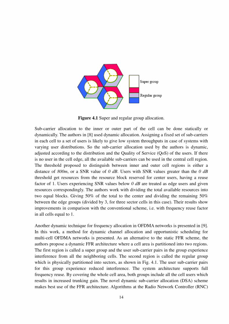
A frequency reuse scheme for multi-cell OFDMA systems for co-channel interference
reduction is proposed in [8]. Each cell is partitioned into three sectors. All the available sub-
carriers in each cell are divided into two groups. One group, called the super group, is reused
in the central region of the three sectors. Another group, called the regular group, is divided
into three parts with regards to the outer region of the three sectors. The sub-carrier a user
can use depends on the location or the received SINR of the user. Thus, intra-cell interference
is avoided and inter-cell interference is minimized. The allocation of super and regular
groups is shown in Fig. 4.1 for three cells. All the sub-carriers may use the same transmit
power in this scheme. Results show that this scheme can bring higher system throughput and
lower co-channel interference (CCI) and it can also increase the data rate at the cell’s edge.
14
Figure 4.1 Super and regular group allocation.
Sub-carrier allocation to the inner or outer part of the cell can be done statically or
dynamically. The authors in [8] used dynamic allocation. Assigning a fixed set of sub-carriers
in each cell to a set of users is likely to give low system throughputs in case of systems with
varying user distributions. So the sub-carrier allocation used by the authors is dynamic,
adjusted according to the distribution and the Quality of Service (QoS) of the users. If there
is no user in the cell edge, all the available sub-carriers can be used in the central cell region.
The threshold proposed to distinguish between inner and outer cell regions is either a
distance of 800m, or a SNR value of 0 dB. Users with SNR values greater than the 0 dB
threshold get resources from the resource block reserved for center users, having a reuse
factor of 1. Users experiencing SNR values below 0 dB are treated as edge users and given
resources correspondingly. The authors work with dividing the total available resources into
two equal blocks. Giving 50% of the total to the center and dividing the remaining 50%
between the edge groups (divided by 3, for three sector cells in this case). Their results show
improvements in comparison with the conventional scheme, i.e. with frequency reuse factor
in all cells equal to 1.
Another dynamic technique for frequency allocation in OFDMA networks is presented in [9].
In this work, a method for dynamic channel allocation and opportunistic scheduling for
multi-cell OFDMA networks is presented. As an alternative to the static FFR scheme, the
authors propose a dynamic FFR architecture where a cell area is partitioned into two regions.
The first region is called a super group and the user sub-carrier pairs in the group experience
interference from all the neighboring cells. The second region is called the regular group
which is physically partitioned into sectors, as shown in Fig. 4.1. The user sub-carrier pairs
for this group experience reduced interference. The system architecture supports full
frequency reuse. By covering the whole cell area, both groups include all the cell users which
results in increased trunking gain. The novel dynamic sub-carrier allocation (DSA) scheme
makes best use of the FFR architecture. Algorithms at the Radio Network Controller (RNC)

15
and the base station are implemented. At the RNC, sub-carriers to the groups are allocated so
that the system performance is increased while satisfying the sum of the minimum
performance requirement of those groups. At the base station, opportunistic scheduling
decisions are made and sub-carriers are assigned to the users.
The research work in [10] provides an analysis of the inter-cell interference coordination in
multi-cellular OFDMA system. The work is based on the FFR technique i.e. partitioning the
cell into two regions (inner and outer). The regions have different frequency reuse factors.
The resource allocation and interference coordination are considered jointly. The problem is
formulated as a combined integer and linear continuous optimization problem and solved by
the Prima Dual Interior Point Method. The best configuration was found in reserving 32
chunks to the interior cell region, and 18 chunks to be shared among the three neighboring
cells (out of the total 50 chunks). The optimal interior cell region radius is determined to be
equal to 2/3 of the overall cell radius. Also the resource distribution is such that 64% of the
resources are kept for the inner cell users and 36% to be divided between the outer cells.
A graph based framework for dynamic FFR in multi-cell OFDMA networks is proposed in
[11]. The dynamic feature provides the capability of adjusting the spectral resources to
varying cell load conditions. The adaptation is accomplished via a graph approach in which
the resource allocation problem is translated to a graph coloring problem. The aim of the
dynamic allocation is to deliver higher cell throughput and service rate in asymmetric cell
load conditions.
A non-conventional technique for frequency allocation for OFDMA networks is proposed in
[12]. The authors stress the fact that previous research done on FFR has focused on relatively
small networks and standard hexagonal shaped cell layouts. For real life networks, with
highly irregular cell layout variation in radio propagation, using a conventional approach is
inadequate. The authors propose an FFR scheme for irregular cellular structure in OFDMA
networks. They also point out that FFR-3 is not an optimal solution for irregular cells as the
number of neighbors for each cell could be different. Furthermore, an allocation algorithm
has been devised for the number of sub-bands for the edge users of every cell. Using data
from real networks of Lisbon and Berlin, it is demonstrated that better throughputs are
achieved for cell edge users, and it is sometimes optimal to split the cell edge band into more
than the standard three sub-bands.

16
Chapter 5
Simulation Platform
5.1 Choice of Simulation Tool
There are a number of different simulation platforms available for simulating wireless
networks and the analysis of different protocols. However, these simulation tools provide
little support for the simulation of different techniques for frequency reuse on a system level.
We have considered tools such as NS-2, OPNET modeler and MATLAB for the simulation
purposes before choosing the Open Wireless Network Simulator (OpenWNS).
NS-2 is an object-oriented event-driven network simulation tool. It is an open source tool and
its main core is based on C++. The programming language used as a front end for simulation
configurations is oTCL. NS-2 can be used for protocol design, traffic studies, protocol
comparison etc. A variety of IP networks can be simulated in NS-2. A large number of
applications, network elements, network types and traffic models are supported by the tool.
Several transport and MAC layer protocols along with different types of traffic sources,
queue management mechanisms are also supported. Scenarios based on various
telecommunication technologies like General Packet Radio Service (GPRS) [13],
Multiprotocol Label Switching (MPLS) [14], AdHoc networks [15], and IPv6 [16] can be
implemented and analyzed.
NS-2 is more concentrated on the protocol analysis and design of protocols and on the
overall systems. Although it is possible to have control over the mobility patterns and
propagation models, the implementation of OFDMA at the modulation level is very simple.
NS-2 does not focus in detail on the assignment of frequency sub-bands to cells. Also, the
logical division of cells into inner and outer regions having different frequency bands is not
supported. Only frequency reuse-1 can be modeled by default. NS-2 add-on for IEEE 802.16
model supports multi-cells to have different frequencies in different cells but still logical
division of cells to inner and outer regions is not possible.
OPNET is another popular choice for modeling and simulation of communication networks,
devices and protocols. It is a commercial tool and is based on object-oriented modeling
approach and graphical editors. Higher OSI layers are the focus of this tool and the lower
layers such as the physical layer and the transmission characteristics are modeled quite
simply. Although a special model is available in the OPNET modeler for WiMAX

17
simulations (WiMAX uses OFDMA) which supports multiple cellular networks, multi-
sectored base stations, path loss modeling, scheduling for uplink and downlink connections
but it is not possible to logically define inner and outer regions in cells. Also, OPNET is not
open source so to additionally include this functionality is not possible. By default, the
OPNET modeler supports hexagonal cells and support for irregular cells is not provided.
After thorough search for research papers on FFR, OpenWNS was found to be one open-
source simulation tool in which some simulations on soft frequency reuse were performed
recently [17]. OpenWNS has a separate module for OFDMA network simulations with some
example scenarios as well. Fine control over the base station parameters, their antenna
transmission powers and azimuth, allocation of sub-bands to base stations is provided. As it
is an open source tool, changes can be made to modify the module according to one’s own
requirements. Also, an important factor in choosing OpenWNS was the possibility of creating
irregular cell patterns over the service area.
5.2 Open Wireless Network Simulator (OpenWNS)
The simulation platform used to perform desired simulations in this thesis is Open Wireless
Networks Simulator (OpenWNS) which is available at [18]. It was developed at the
Department of Communication Networks (ComNets) at RWTH Aachen University. It is an
event driven simulation tool for the simulation of various networks and technologies. The
core programming language is C++ while python is used for configurations and simulations.
Fig. 5.1 shows the OpenWNS framework.
For the simulations we required a tool which can allow us to make irregular cellular patterns
and allow allocation of frequency sub-bands to cells. The tool also needed to provide
propagation models, mobility models and traffic models to simulate real-time environments.
Most of the required features are available in OpenWNS, and some of the changes were
made to the simulator to incorporate the functionality necessary for the simulations. For
example, OpenWNS does not support the feature of frequency allocation to inner and outer
cell regions (required for FFR) which had to be added in the simulator.
5.2.1 Event Scheduler
Both real time and non-real time schedulers are provided in OpenWNS. Real time scheduler
is for building demonstrators and for implementing interaction with the simulation host. Non-
real time scheduler, used for the simulations in our case, is a two layered map data structure.
For a distinct simulation time, a map entry is created. In every map entry, there is a queue of
all the events that are scheduled to run at that time.
18
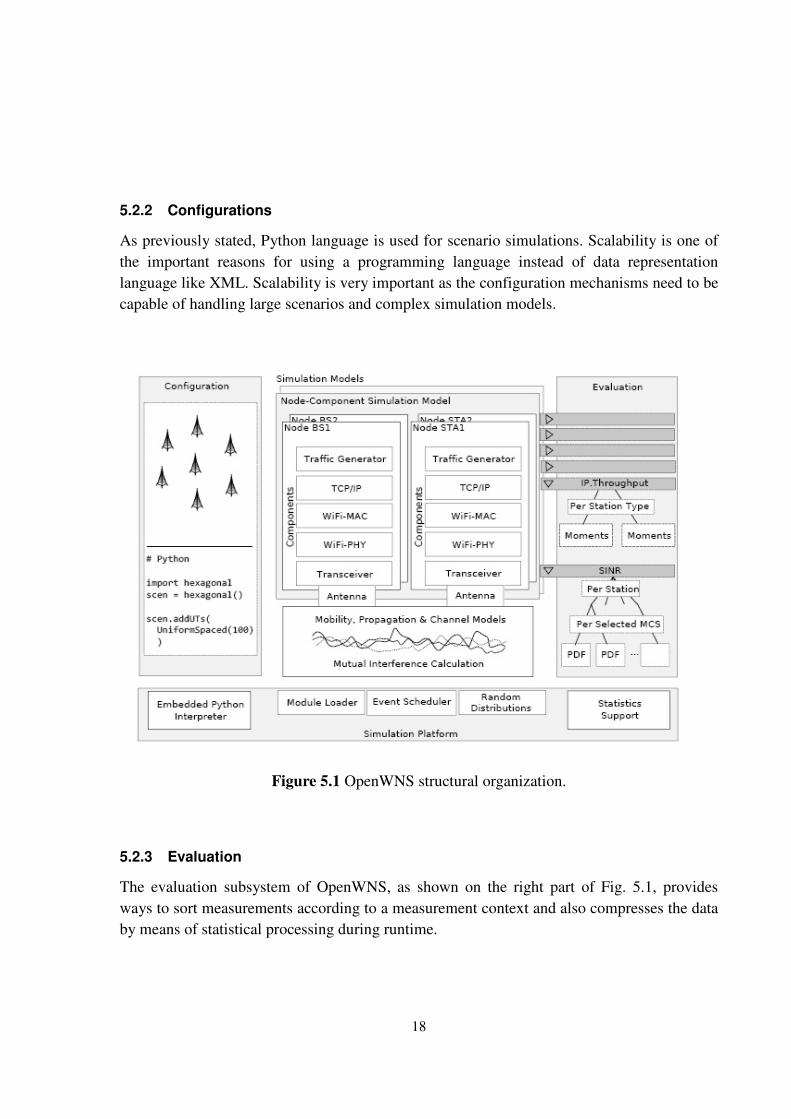
5.2.2 Configurations
As previously stated, Python language is used for scenario simulations. Scalability is one of
the important reasons for using a programming language instead of data representation
language like XML. Scalability is very important as the configuration mechanisms need to be
capable of handling large scenarios and complex simulation models.
Figure 5.1 OpenWNS structural organization.
5.2.3 Evaluation
The evaluation subsystem of OpenWNS, as shown on the right part of Fig. 5.1, provides
ways to sort measurements according to a measurement context and also compresses the data
by means of statistical processing during runtime.
19
When configuring simulation scenarios, measurement parameter can be chosen from a
number of different kinds of evaluations as desired by the simulation. For example, an
evaluation of the signal to interference noise ratio (SINR) measurement could be configured.
5.2.4 Simulation Modules
OpenWNS provides support for various technologies standards. For the data link layer,
WiMAX and WiFi are available in the simulator. OpenWNS allows for multi-standard nodes
which can operate concurrently below the IP layer. TCP and UDP are the available standards
for the transport layer. Traffic models are also available which can operate on top of either
transport, network or data link layer.
One of the main simulation modules is RISE (Radio Interference Simulation Engine). It
manages node mobility and interference calculations. The total received signal strength for
every transmission is calculated by the channel model using the formula in (5.1)
P
R=P
T− L
path− L
shadow− L
FastFading+G
T+G
R (5.1)
Here PR is the received power, PT is the transmitted power, Lshadow is the loss due to
shadowing, LPath is the path loss, LFastFading is the loss due to fast fading, GT is the transmit
antenna gain and GR is the received antenna gain. The parameters are measured in dB/dBm
scale.
Antenna models are also an important part of the simulation modules. Two main types of
antennas are notable i.e. omni-directional and beamforming antennas. Omni-directional
antenna is defined by its gain in all directions, and beamforming antenna allows the user to
dynamically adjust antenna’s directivity by varying the vertical angle θ and azimuth angle φ
of the antenna.
A. Path loss Models
Several path loss models add to the feature of calculating path loss between the transmitter
and receiver in the OpenWNS simulator. Constant, free space, single slope and multi slope
models are available. Constant path loss model is not an accurate model for real scenarios but
is sometimes used for very short or very far distance for which the loss can be assumed
constant.
Free space is the term used for mediums in which the signal can propagate without
obstruction between the transmitter and receiver. The free space model is a good
approximation for satellite communication systems and for microwave LOS links, when the
transmitter and receiver are high above the ground. Friis Formula gives the free space loss as
20
2
4
=
dLPath
π
λ , (5.2)
where LPath is the free space loss, λ is the wavelength and d is the distance between
transmitter and receiver. We can see from (5.2) that doubling the distance or carrier frequency
increases the path loss by four times or 6 dB.
The single slope model is defined as
η
π
λ
=
dLPath
4 , (5.3)
where LPath is the path loss, d is the distance between the transmitter and receiver, λ is the
wavelength and η is the propagation constant. When η = 2, it is same as the free space model.
The multi slope model is defined by using a path loss factor η1 after some distance d0 and up
to a critical distance dc, after which the power falls with path loss factor η2. Pt is the transmit
power and K is the antenna gain of both transmitter and receiver side.
−−+
−+=
)/(log10)/(log10
)/(log10)(
1020101
0101
cc
rddddKPt
ddKPtdBdP
ηη
η
c
c
dd
ddd
>
≤≤0 (5.4)
(5.4) gives the path loss in dB scale. Multi-slope model can be extended to more than two
regions [19].
B. Traffic Model
The OpenWNS traffic model is named Constanze. Traffic generators create data packets and
can be connected to any of the transport, network or data link layers. Available traffic models
in OpenWNS are Simplistic Point Process (PP), Markov-Modulated Poisson Process
(MMPP) and Autoregressive Moving Average (ARMA).
PP models include Constant Bit Rate (CBR) and Poisson traffic. CBR traffic model is very
basic and is used for connections that transport traffic at a constant bit rate. It is well suited
for any data type for which the end systems require predictable response time and a specific
bandwidth is available for the duration of the connection. This model can be used for

21
simulating video conferencing, telephony or any on-demand service such as interactive video
and audio. In this model, time synchronization between the source and destination is
considered.
Poisson traffic model is based on the memory-less Poisson distribution and is used to model
traditional telephone networks. In this model, the number of incoming data packets follow
the Poisson distribution.
The formula for the Poisson probability function is given as:
!),(
x
exP
xλλ
λ−
= for x = 0,1,2…, (5.5)
Here λ is the average rate of packet arrival in a given time interval, x is the number of
occurrences of an event and P(x, λ) is the probability of the occurrence. Two characteristics
of Poisson generated data is that the arrivals occur in an orderly manner i.e. no two
occurrences can be simultaneous and secondly, each occurrence is independent from the
previous one.
MMPP is a Poisson process with variable rate. Its current rate λi is controlled by a
continuous-time Markov chain. Research has shown that classical Poisson methods are
insufficient for large scale networks, which is where MMPP comes in handy [20]. It is able to
model traffic activity well, keeping the approximations scalable [21]. Further, MMPP can
model traffic bursts and arrival streams more accurately than other models.
MMPP can be represented by two matrices P and Ʌ where P is the generator matrix of
Markov process and Ʌ is a diagonal matrix giving the arrival rate for each state of the
Markov process.
−
−
−
=
mmmm
m
m
www
www
www
P
L
MOMM
L
L
10
11110
00100
(5.6)
Λ=Diag [λ0 λ1 . .. λm ] (5.7)
Here wij gives the state transitions from one state to another and λi is the current arrival rate. For
detailed study of MMPP, the readers are referred to [22].

22
ARMA model can be used to generate random data sequence with a given autocorrelation or
power spectral density. It can also be used to predict into the future about network traffic.
Given a time series of data, the ARMA model is a tool for understanding and predicting
future values in the series. ARMA is composed of two parts, an autoregressive (AR) part and
moving average (MA) part, as shown in Fig. 5.2.
The AR model is an all pole model and MA is an all zero model, which makes ARMA a pole
and zero model. Mathematically, ARMA can be written as
∑∑ −− +−q
=i
iti
p
=i
ititt εθXε+c=X11
φ (5.8)
Where φ i (i = 1,2…p), θi (i = 1,2…q) are the parameters of the ARMA(p,q) model, c is a
constant, εt and εt-i are white noise, and Xt is the data sequence.
Figure 5.2 ARMA model.
In addition to all the above mentioned models, OpenWNS also provides separate modules for
the simulation of Wi-Fi (IEEE 802.11), WiMAX (IEEE 802.16) and TCP/IP. Also, another

23
module named WiMAC (WiMAX Medium Access Control) exists which supports the
OFDMA and hence is the module used to run the simulations for this thesis.
Although all these modules are available in OpenWNS for users to configure and analyze
their desired wireless scenarios, but a major hurdle in using these models is the lack of
available documentation. Till now, OpenWNS has a very limited documentation set which
gives difficulties to the users in properly understanding and using all the available models.

24
Chapter 6
Optimization of FFR for Irregular Cellular Structure
6.1 Frequency Reuse Schemes
The frequency reuse schemes simulated in this thesis are:
• Frequency Reuse-1
• Fractional Frequency Reuse-3 with Random Frequency Allocation (FFR3-RFA)
• Fractional Frequency Reuse-3 with Algorithmic Frequency Allocation (FFR3-AFA)
6.1.1 Frequency Reuse-1
In frequency reuse-1 scheme or simply reuse-1 scheme, the total system bandwidth is
available to be allocated in each cell. In traditional GSM systems, reuse-1 is almost
impossible to achieve because the users would come up against severe adjacent channel and
co-channel interferences. In OFDMA networks, as the subcarriers are orthogonal to each
other, interferences from other subcarriers are alleviated but inter-cell interference at cell
edge is higher which results in weak signal strength for users at the cell edge. This means,
users close to the base station may get very high data rates with minimum interference, but
the users close to cell edges experience degraded quality because of the same frequency sub-
bands being used in the neighboring cells by other users.
6.1.2 FFR-3 with Random Allocation
In FFR-3, each cell is logically partitioned into center and outer areas based on fixed distance
threshold or signal to noise ratio (SNR) threshold. The edge users of neighboring cells are
assigned different frequency sub-bands so that they do not interfere with each other. Three
sub-bands are reserved for allocation in cell edges. 30% of the total bandwidth is reserved for
the edge users. The 30% is divided into three groups. Hence each sector’s edge has 10% of
the total bandwidth. For the simulations, the region beyond the 2/3 of the cell radius is
considered as the outer region or the cell edge. Since the irregularity of the cell is achieved
by changing the power and the antenna tilt of the sectors, users are placed by looking at the
coverage of each sector. In this allocation scheme, the three frequency sub-bands were
randomly assigned to cell edges of each cell sector without considering neighbor relation or
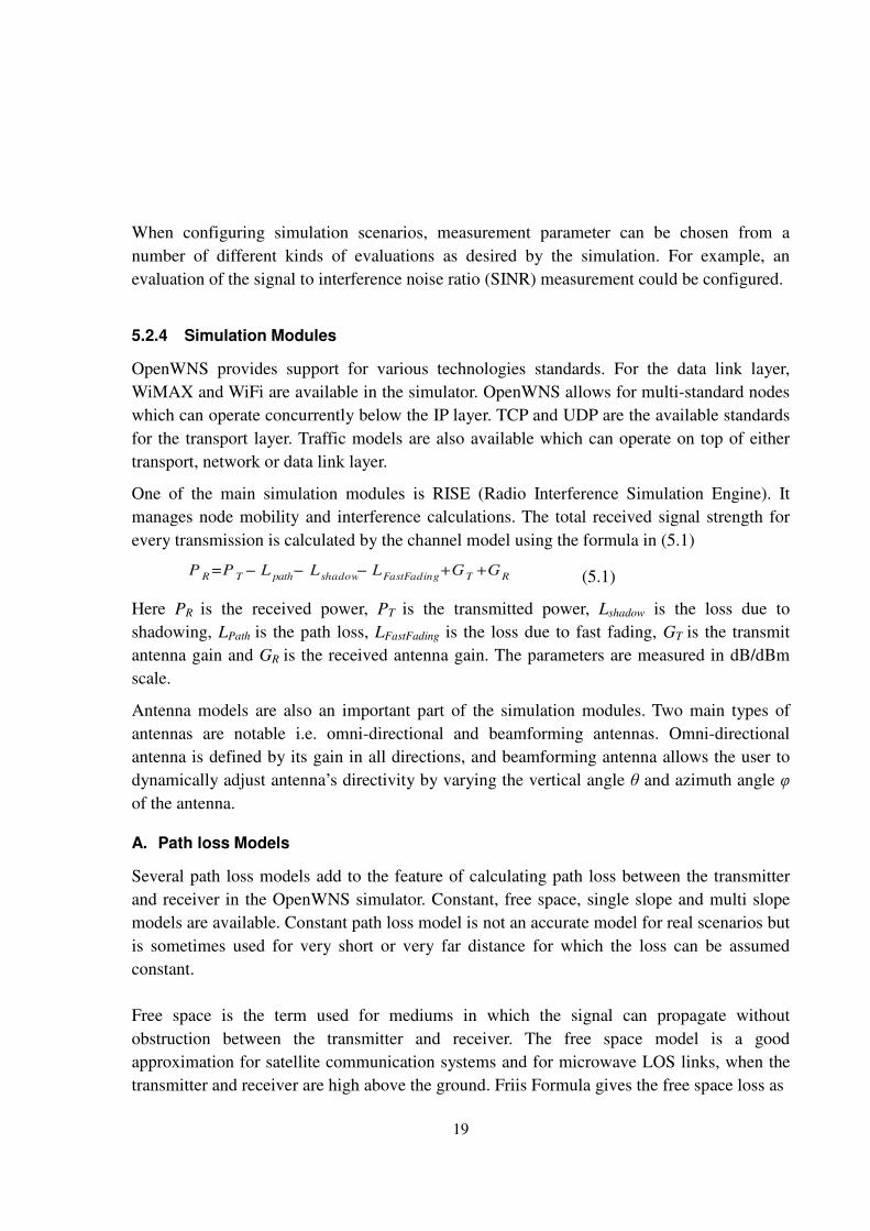
25
overlap between coverage of cell sites. Random allocation is used to clearly demonstrate the
difference between a poor frequency allocation to cell edges and the algorithmic allocation,
to be presented in the next section.
Figure 6.1 Same sub-bands in neighboring cells in FFR3-RFA.
Fig. 6.1 shows sectors for three separate cells getting assigned frequency bands randomly. As
seen from the figure, the random allocation could result in a situation where two neighboring
cell edges are assigned the same frequency band. This will not lower the interference for the
cell edge users in such cells.
6.1.3 FFR-3 with Algorithmic Allocation
The second frequency allocation scheme that we used for the simulations is FFR-3 with
algorithmic frequency allocation. The algorithm’s objective is to optimize the cell edge
performance. The main idea is that instead of randomly allocating sub-bands, cell edges are
assigned frequency sub-bands by taking into consideration the allocated sub-bands to cell
neighbors as well as the degree of overlap between the neighboring cells. By introducing
these constraints, close to real-life scenario for frequency allocation was attempted.
The optimization procedure aims to further improve the throughput achieved by cell edge
users. In other words, the frequency sub-bands are allocated to cell edges in such a way that
same sub-bands are kept as far as possible. To emphasize the need for optimization, let us

26
consider an example. Suppose we have a large cell A which has many smaller cells as its
neighbors. If only three frequency sub-bands are available for allocation to cell edges, there
is a possibility that one of the neighbors of cell A will end up having the same frequency at
its edge as the large cell A’s outer region. This is where optimization comes into play because
we know that a collision is inevitable. We can shift this collision such that the overall damage
is minimum. For example, cell C, a smaller cell neighboring to A, has been allocated the
same cell edge frequency as that assigned to the cell edge of cell A. We assume that cell C
and cell A have a large overlap area. It would be a better solution to assign the conflicting
sub-band to some other neighbor of cell A that has a lesser overlap area than the overlap area
of cell A and cell C. This will lead to less interference for users in the overlap regions of cells
A and C, and hence improved overall throughput for the system.
In the algorithm considered in this thesis, the optimization procedure assumes the amount of
cell overlap as a factor for re-allocation of frequency sub-bands to edge users, instead of
directly considering user throughput at cell edges. This is done due to the limitations of the
simulation tool (OpenWNS). Cell overlap directly affects the user throughput because if the
overlapping part of two cells have same frequency sub-band then the users within the overlap
area will most likely have degraded signal quality. The algorithm tries to make sure that cells
with significant overlaps do not end up having the same frequency allocation.
Fig. 6.2 shows a Matlab representation of cells to give an idea about the overlap and cellular
structure used. The figure clearly shows the overlap between cells with different colors for
each cell. Because of the irregular cell patterns in real-life networks, coverage holes within
the cellular network may also exist where there is no coverage at all. Expert cell planning is
required to reduce these holes to a minimum. The cell boundaries shown in Fig. 6.2 are not
exact because for real networks there is no definite boundary of a cell.

27
Figure 6.2 Cell overlap.
For the algorithm, the input is the cellular network’s information. Network information
includes the overall cellular configuration and the degree of overlap among the cells. The
cellular configuration will give us the neighbor relationships for each cell and the degree of
overlap will aid the optimization procedure for frequency allocations. This information is in
the form of two matrices of size NxN where N is the number of cells. Each row of the
matrices gives the information of a cell’s neighbors and non-neighbors. The first matrix is the
connectivity matrix which gives the neighbor relationship of each cell. A “0” represents no
neighbor connection and “1” represents a neighbor. An example for this matrix for a three
cell network is shown in Fig. 6.3 where A, B and C are the three cells. In this case, the
neighboring cell of A is only B as it has a 1 at B’s position. An element aij in the matrix for
i=j will always be zero because a cell cannot have itself as a neighbor, with i referring to
rows and j referring to columns in the matrix.

28
A B C
Connectivity matrix → a =
010
101
010
C
B
A
Overlapping matrix → a =
0250
5010
0150
Figure 6.3 Input matrices for the algorithm.
The second matrix is the overlapping matrix which tells us the degree of overlap between the
neighboring cells. In the algorithm, the degree of overlap is defined by integers between 0
and 100, where 0 means no overlap or no neighbor overlap and 100 is full overlap i.e. two
cells on top of each other. All other values will lie within this range according to the overlap
among two cells. The values between 0 and 100 are easier to set because we can relate these
values to the percentage of areas (based on signal strength) being overlapped for each cell.
The overlapping matrix is also shown in Fig. 6.3 with sample values. The value of 10 at
position a21 means that 10% of the total coverage area of cell B is overlapped with cell A.
This does not mean that cell A is also overlapped with cell B by the same amount. The
overlap area is relative to the cell size. This is clear from the overlapping matrix that the
value at position a12 is 15, meaning that because of the overlap between cell A and B about
15% region of cell A is in overlap with cell B. In our case, connectivity and overlapping
matrices are kept in a text file and from there read into the program routine.
Apart from these two input matrices, the number of frequency sub-bands which are to be
divided among the cells can also be taken as an input. For simulating FFR-3 with optimized
allocation, the frequency set consists of three sub-bands and is implemented as an array with
three values each referring to a sub-band, as given in (6.1).
[ ]321=f (6.1)
The algorithm can take more number of sub-bands as input, but it is not studied in this thesis.
Once the inputs are defined, we move onto the frequency allocation part. The frequency
allocation is done in two steps. First, there is a random allocation of sub-bands to cell edges
and then the edges which require optimization are treated further. The steps are as follows:
Initially, all the cells are assigned a frequency sub-band value of -1. A random frequency
band fi is assigned from the frequency set f to cell k. For cell k, we find all the cells that are
connected to it by going through the kth
row of the connectivity matrix and locating all the

29
ones in that row. Frequency bands of all the neighbor cells are then checked. Initially,
because of the arbitrary value assigned to each cell, cell k will have a different frequency
band allocated than its neighbors, but as the algorithm proceeds and more and more cells are
assigned frequency bands, it is likely that adjacent cells have same sub-band due to random
allocation. If one or more neighbors have same frequency sub-band allocated as k then the
cell k is assigned another frequency sub-band from the frequency set f. If that band is also
allocated to some neighbor then the next frequency sub-band from the set is assigned and
checked for the interference. If there is no frequency sub-band that has not been allocated to
the neighboring cells, the frequency sub-band that was last assigned is kept and would be
changed, if required, when considering the overlapping between cells in the next step. These
frequency allocations are stored in a matrix whose rows are equal to number of cells and each
column position gives the allocated frequency sub-band for that cell.
After this first allocation, each cell is re-visited again; neighboring cells are located from the
overlapping matrix along with their corresponding overlapping values. If for a particular cell,
there is no neighboring cell with the same frequency sub-band, we move onto the next cell.
Once a cell k is reached whose neighbor j has the same frequency sub-band assigned,
overlapping factor value akj from the overlapping matrix is checked. If that value is larger
than a threshold value, we need to change the frequency sub-band for cell k. For the thesis, a
threshold value of 10 is used i.e. if the cell overlapping is 10% or more then we change the
allocation for cell k. We assign that frequency sub-band of the neighboring cell for which cell
k has minimum overlapping value. This process is repeated for each cell, and all cells are
tested against their neighbors considering their overlapping values. Each cell is visited a
number of times to make sure that cells with high overlap value never have the same
frequency sub-band. As frequency sub-bands are limited, two lightly overlapped cells could
end up having the same frequency sub-band in their cell edges. The end result of the
algorithm is a matrix which gives the revised allocation of frequencies.
The pseudo-code for the algorithm is given below:

30
FFR(number of cells, number of sub-bands available for outer cells)
Load connectivity matrix from file
Load overlapping matrix from file
For each cell
Assign a dummy value (suppose -1) of sub-band
End for
For each cell
Assign a random sub-band from the frequency set f
FindNeighbor(current cell k) // identify neighbors for each cell
For each neighbor
Check the sub-band of the neighbor
If (neighbor has same sub-band allocated)
Assign another sub-band from the frequency sub-set f and
check again
End if
If (all sub-bands are allocated to neighbors)
Do nothing i.e. the last assigned sub-band is kept
End if
End for
End for
For I = 5 iterations
For each cell
If(no neighbor cell has same sub-band allocated)
Do nothing
End if
Else // neighbor has same sub-band
If(overlapping factor value for that neighbor > threshold
value)
sub-band of the current cell = sub-band of the neighboring cell
with least overlapping factor
End if
End else
End for
End for
END FFR
31
One important point to note is that in the second loop of the pseudo-code, the values assigned
to a cell are fixed in the progression of the loop. Any changes made in the neighboring cells
of an already assigned cell c, does not change the value of cell c.
Setting the threshold value can have significant effects on the frequency allocation. If this
value is set too high then it is possible that many overlapping cells with same frequency sub-
band are skipped and are not optimized. As a result, cell edge users of many cells could still
experience degraded service. On the other hand, if the threshold value is set too low there
will be more cells which would require optimization. Because of the limitation on the
number of frequency sub-bands, it would not be possible to enhance performance for all such
cells. Optimized results are not expected if most of the cells in the network are heavily
overlapped.
To locate all the neighboring or connecting cells for a given cell, the FindNeighbor method
simply finds the non-zero value in each row of the NxN matrix (where the neighbor
information is stored).
If we consider increasing the number of sub-bands, although the inter-cell interference
between the cells will certainly be reduced but it will also have its consequences. With
increasing number of sub-bands, bandwidth of each sub-band will be reduced and this
reduced bandwidth can have the effect of lowering the throughput for cell edge users. And
also with large number of sub-bands for cell edges, there is a possibility of not utilizing the
full resources because of the fact that frequency reuse factor will be much higher for cell
edge users in that case.

32
Chapter 7
Simulation Setup and Results
7.1 Simulation Model and Parameters
The simulation parameters are summarized in Table 7.1.
Parameter Value
System Bandwidth 20 MHz
No. of Base
Stations
21
System
configuration
OFDMA
OFDMA Symbol
duration
102.858 µsec
Packet Size 2400 bits
Downlink Traffic 100 Kbps and 1
Mbps , CBR
Frame Length 10 ms
Cell Radius Variable
FFT size 2048
Sub-carriers 96
Table 7.1. Simulation parameters.
The simulation model consists of 21 base stations each with its own coverage pattern. The
cells formed are non-hexagonal. Irregular cells were created by varying the transmit powers
of base stations. For the simulations, transmit power ranges from 20 dBm to 45 dBm. The
coverage patterns for cell sites are shown in Fig. 7.1. Users were made to traverse the whole
scenario, and then their SNR and serving base station were studied to plot the radiation
pattern. The dots, in Fig. 7.1, are the users having received signal strength above a threshold

33
value and the different colors indicate the different sectors. The received signal strength of -
95 dBm is taken as the threshold value (cell boundary). The white lines were added later on
to make the sectors and the shape of the cell clear. Transmit powers 30-40-30 means that the
transmit power is 30 dBm in the first sector, 40 dBm in the second sector and 30 dBm in the
third respectively. Apart from transmit power; down tilt and azimuth of antennas are two
other parameters which could be used to introduce irregularity to cells. The azimuth angles
for antennas were set to 30o, 150
o and 270
o. Changes to the azimuth angle and the down tilt
of the antennas results in different irregular cell patterns.
OpenWNS does not support the feature of frequency allocation to inner and outer cell regions
by default, and this functionality had to be added to the simulator. Frequency ranges are
masked out depending on the FFR scheme being used. Masking out frequency ranges meant
that the range would be made unavailable for the base station to use.

34
Figure 7.1 Cell radiation patterns for four base stations with transmit powers of 20-20-20,
45-30-20, 30-40-30 and 40-40-40. Note: sector-1 is on left hand side, sector-2 is at
top right and sector-3 at bottom right.
Frequency division for FFR-3 is shown in Fig. 7.2. In our simulations, the transmit power of
the base station is the total power used for both the center and the edge.

35
Figure 7.2 Frequency division between cell centre and cell edges.
7.2 Choosing Cell Edge
Based on the work performed by Assaad in [10], the area beyond 2/3 of the total cell radius is
considered as cell edge no matter what the size of the cell. Work done in [10] shows that the
optimal interior cell region radius is determined to be equal to 2/3 of the overall cell radius.
In our simulations we are not considering or generating traffic for users closer to the base
station than the 2/3 cell mark. All the users are placed manually beyond that point. Adding
users to the center regions will not affect the performance of the edge users as they have
different frequency chunks assigned to them. There is also an option to set an SNR threshold
to establish cell edge but it is not used since one user per base station is simulated, and also it
is easier to place the user at a position beyond the 2/3 region than to find the correct position
in the cell where the received SNR of the user is below the threshold. One user per sector is
simulated for a number of reasons. Firstly, this way the location of the interferers is known
and secondly, simulating with a large number of users was resulting in a very large
simulation time.

36
7.3 Analysis of Results
7.3.1 Number of Users and Placement
The number of edge users is relatively low in total, for 21 base stations there are 21 users.
But the downlink traffic from their base stations is such that the complete bandwidth is
utilized. The users are placed closer to the edge of the cells, sometimes ending up in the
overlap region between two cells. They are not mobile as this makes it easier to know which
cell the user is connected to and understand the results. Random mobility introduces
ambiguity as many users could end up in the same cell, whereas some cells could be left
completely empty. There was one user per cell edge region for each base station. The number
of users could be increased but it would not affect the overall trend of the results.
7.3.2 Packet Throughput
The throughput is calculated as a ratio of packets received to the packets sent at the listener.
The results are in form of percentages which tells us the percentage of successfully received
packets by the user as compared to total number of packets sent. This is comparable to
throughput which is the average rate of successful packets/bits delivered over a
communication channel. The allocation is focused on improving the overall throughput of the
system and individual user throughput is not directly considered. As mentioned earlier, the
link is tried to be fully utilized so that there are no free resources. This gives the system high
interference, and hence makes the difference between the different allocation schemes clear.
Results are given in Table 7.2. In case of random allocation, as predicted, the similar sub-
bands in neighboring cells interfere and result in lower throughput values.
7.3.3 Effects of Irregular Cells
In regular hexagonal cells scenarios each sub-band is reused at constant distances from each
other and hence the interference created for the users is almost the same throughout the
scenario. Irregular cells results in varying interference over the cell area. This changes the
dynamics of frequency allocation.
7.3.4 Implications with Regards to Real Network Scenarios
In real scenarios it is very rare that there is a perfect hexagonal cellular structure. While using
frequency reuse techniques the cellular structure makes a difference. As seen from the results,
smart frequency allocation shows significant improvements with regards to throughput in

37
such irregular scenarios. Introducing more factors into the frequency allocation assignment
method can give better results for larger and more complex network.
In the different simulation runs, the user positions were changed slightly and the results were
studied. When the frequency sets are allocated by considering the neighboring cell edge sub-
bands and overlap conditions of the network, a clear increase in throughput compared to the
other two schemes for the edge users is observed in Table 7.2. The increase in throughput for
FFR with algorithmic allocation is due to the fact that the scenario is irregular and high
interfering base stations are kept as far from each other as possible in sub-band allocation.
This results in better throughput for the edge users. In the FFR schemes, although the
bandwidth at cell edge is less than the reuse-1 scheme but the interference is much more
significant in reuse-1. That is why user data rates for reuse-1 are considerably less than the
FFR-3 schemes for cell edge users. In the reuse-1 scheme, the cell edge users are much more
interference-sensitive than bandwidth-sensitive. At low downlink data rate, FFR-RFA and
FFR-AFA have similar results. To see the difference clearly between the two allocation
schemes, high downlink data rate of 1 Mbit/sec were tested. The overall throughput was
lower but the difference between them is more evident. The reasons why the two schemes
have same similar results at low data rates are explained later on.
Run Reuse-1 FFR3 with Random
Allocation
FFR3 with Algorithmic
Allocation
1 50.12% 65.44% 66.83%
2 49.75% 64.55% 66.60%
3 49.95% 64.80% 66.12%
Table 7.2.a Throughput for edge users with 100 Kbit/sec downlink.
Run Reuse-1 FFR3 with Random
Allocation
FFR3 with
Algorithmic Allocation
1 28.45% 31.44% 37.83%
2 28.76% 31.55% 37.60%
3 28.83% 31.80% 37.12%
Table 7.2.b Throughput for edge users with 1 Mbit/sec downlink.

38
7.4 Scenarios
Fig. 7.3 shows the simulation scenario with algorithmic allocation. The three different colors
represent the three frequency sub-bands used for cell edges in different sectors of the cells.
The dark regions are the overlapping areas between the neighboring cells.
Figure 7.3 Simulation scenario.
Fig. 7.4 shows how the allocation of each sub-band is kept as apart as possible. This is
mainly done by checking the neighbors and finding a sub-band not allocated to the
neighboring cells.

39
Figure 7.4 Allocations of each sub-band is kept as far away as possible as the algorithm goes
through the scenario.
In the scenario shown in Fig. 7.5 an interesting case occurs. Base station numbered 4 has
neighbors of all three sub-bands. In this case the overlap plays an important role. We see the
region outlined in black has the maximum cell overlap. Overlap between base station 1 and
base station 4 is lesser and the overlap between base station 2 and base station 4 is the
smallest. Therefore, the algorithm allocates the same sub-band to base station 4 and base
station 2. This also results in base stations 6 and 7 having the same sub-band. If base station 6
was given the green sub-band, it would cause greater overlap with base station 3. Hence it is
assigned the blue sub-band causing lesser overlap with base station 7. The algorithm
automatically converges itself to this situation.

40
Figure 7.5 The impact of overlap while allocating sub-bands. The black out-lined area is the
maximum overlap area.
Fig. 7.6 shows the user placements. In cell sectors marked 3 and 4, the users are in the
overlap region. This will cause more interference in case neighboring cell sectors have
similar sub-bands allocated to them. In case of random allocation, cell sectors 3 and 4 have
the same sub-band. Since we are simulating one user per base station, it is important to know
where and how they are placed, especially in the cells where overlap is an important factor in
the allocation of the sub-bands. Users in sectors 2, 3 and 4 are placed around the 2/3 mark.
The users in sectors 3 and sector 4 are in the overlap region as shown in the figure. Only the
frequency allocation to cell sector numbered 4 is changed. Cell sectors 3 and 4 have the same
frequency for that simulation.
1
2
3
4 5
6
7

41
Figure 7.6 Scenario with user placement.
Data rate of 1 Mbit/sec was used in the downlink for all scenarios. It was essential because at
lower rates both users in the overlap region could end up being connected to the same base
station and not create any interference to each other. This is also why FFR-RFA and FFR-
AFA have similar results at lower downlink data rates. In a high downlink data rate, if both
users try to connect to the same base station they will have to compete for resources, and if
they connect to separate base stations they will create interference for each other.

42
Chapter 8
Conclusions and Future Work
8.1 The Algorithm
The algorithm used for allocating the frequency bands achieved better results than the other
allocation schemes, although a larger scenario would be more desirable to demonstrate the
frequency allocation process. However, five interferers for each frequency band are sufficient
to get reasonable interference and results. A literature study was done regarding search
methods that could be used in the algorithm. Our algorithm was made specifically for
scenarios with irregular cells and with cell overlap regions of varying sizes. This algorithm
can be enhanced by adding other factors into the equation such as cell size. Also the work can
be expanded further to dynamic frequency allocation.
8.2 Choosing a Tool
Choosing a simulation tool was also an important part of our work. There were no off-the-
shelf solutions available for our problem. We chose to work with an open source tool, so that
we could make changes to the code and customize it. But as a drawback there was little help
available regarding the tool.
8.3 The Scenario
The base station positions in the scenario had to be carefully specified to achieve the desired
overlapping effect in the simulator. It was important to have a cell with more than three
neighbors. This would allow us to see the effect of the algorithm on the performance results.
Creating a customized scenario does not mean though that the algorithm will not work for
other scenarios.
8.4 Effect of User Placements
The user placement was done manually in locations with known received SNR so that they
were using the cell edge sub-bands. Since few users were simulated it was important to place
them in the proximity of other users, otherwise the difference in the results for the different
schemes was lesser.

43
8.5 Results
The results obtained were coherent with our expectations. Better throughputs were achieved
for frequency allocation based on our algorithm. Schemes which resulted in minimum
interference resulted in better results. Interference was caused by base stations using the same
frequency sub-bands. It was essential to have a balanced traffic load in the downlink, so that
enough resources were utilized to cause sufficient interference. The results showed that poor
allocation (non-algorithmic) in scenarios of irregular shaped cells with different overlap
regions lead to lower overall throughputs. Similarly for reuse-1 scheme, the high interference
experienced by the edge users significantly reduces the system performance. By using an
algorithmic approach to such a scenario, where cell shape and the overlap between them is
non-consistent, leads to much improved results. This shows that for such scenarios factors
such as cell overlap, user throughput and base station transmit power could be important to
consider while using fractional frequency reuse. These results are specific for FFR-3.
8.6 Future Work
More work is needed in simulating frequency reuse schemes for irregular cell networks.
Larger scenarios can be simulated with various kinds of propagation conditions. In irregular
cell networks factors other than cell overlap can be used to make a frequency reuse scheme,
such as frequency allocation based on user throughput. Also simulations with different
numbers of sub-carriers can also give interesting results. There is also room to test FFR-5,
FFR-7 or FFR-11 schemes in irregular cellular scenarios. It was beyond the scope of our
work due to time limitations.

44
Bibliography
[1] Y. Li, and G. L. Stuber. Orthogonal frequency division multiplexing for wireless
communications. Springer, 2006.
[2] T. L. Singal. Wireless Communications. Tata McGraw-Hill Education, 2010.
[3] M. Bohge, J. Gross, and A. Wolisz. Optimal power masking in soft frequency reuse based
OFDMA networks. European Wireless Conference, 2009.
[4] 3GPP R1-050608. Inter-cell interference handling for E-UTRA. 3GPP-RAN Work Group
1 (WG-1), Meeting #42, UK, 2005.
[5] 3GPP R1-060291. OFDMA Downlink inter-cell interference mitigation. 3GPP-RAN
Work Group 1 (WG-1), Meeting #44, Colorado, 2006.
[6] 3GPP R1-050272. OFDM air interface with QoS at cell edge. 3GPP-RAN Work Group 1
(WG-1), Meeting #40, China, 2005.
[7] 3GPP R1-051341. Flexible fractional frequency reuse approach. 3GPP-RAN Work
Group 1 (WG-1), Meeting #43, Korea, 2005.
[8] H. Lei, L. Zhang, X. Zhang, and D. Yang. A novel multi-cell OFDMA system structure
using fractional frequency reuse. Proceedings of the 18th
International IEEE Symposium
Personal, Indoor and Mobile Radio Communications (PIMRC), 2007.
[9] S. H. Ali, and C. M. Leung. Dynamic frequency allocation in fractional frequency reused
OFDMA networks. Journal of IEEE Transactions on Wireless Communications, volume: 8,
issue: 8, 2009.
[10] M. Assaad. Optimal fractional frequency reuse (FFR) in multicellular OFDMA System.
Proceedings of the 68th
IEEE Vehicular Technology Conference (VTC), 2008.
[11] R. Y. Chang, Z. Tao, J. Zhang, and J. Kuo. A graph approach to dynamic fractional
frequency reuse (FFR) in multi-cell OFDMA networks. Proceedings of the IEEE International
Conference on Communications (ICC), 2009.
[12] L. Chen, and D. Yuan. Generalized frequency reuse schemes for OFDMA networks:
optimization and comparison. Proceedings of 71st IEEE Vehicular Technology Conference
(VTC), 2010.
[13] R. J. Bates. GPRS: General Packet Radio Service. The McGraw-Hill Professional, 1st
edition, 2008.
45
[14] B. S. Davie, and Y. Rekhter. MPLS: Technology and Applications. Morgan Kaufmann,
1st edition, 2000.
[15] P. Mohapatra, and S. Krishnamurthy. Adhoc Networks: Technologies and Protocols.
Springer, 1st edition, 2004.
[16] S. Hagen. IPv6 Essentials. O’ Rielly Media Inc., 2nd
edition, 2006.
[17] Z. Xie, and B. Walke. Enhanced fractional frequency reuse to increase capacity of
OFDMA systems. Proceedings of the 3rd
international conference on New Technologies,
Mobility and Security (NTMS), 2009.
[18] OpenWNS - Open Wireless Network Simulator. Department of Communication
Networks, RWTH Aachen University. Available from: http://www.openwns.org.
[19] E. McCune, and K. Feber. Closed-form propagation model combining one or more
propagation constant segments. Proceedings of the 47th
IEEE Vehicular Technology
Conference (VTC), 1997.
[20] W. E. Leland, M. S. Taqqu, W. Willinger, and V. Wilson. On the self-similar nature of
ethernet traffic (Extended Version). Journal of IEEE/ACM Transactions on Networking,
volume: 2, issue: 1, 1994.
[21] W. Fischer, and K. S. Meier-Hellstern. The Markov-modulated Poisson Process
(MMPP) Cookbook. Journal of Performance Evaluation, volume: 18, issue: 2, 1993.
[22] G. Bolch, S. Greiner, H. de Meer, and K. S. Trivedi. Queuing Networks & Markov
Chains: Modeling and Performance Evaluation with Computer Science Applications. John
Wiley & Sons, Ltd, 2nd
edition, 2006.