Embed Size (px)
Citation preview
Simulating the effects of vegetation and landscape
structure on fire behavior in northeastern Portugal: the
case of holm oak (Quercus rotundifolia)
Soukaina Rachdi
Dissertation presented to the School of Agriculture of Bragança in
partial fulfillment of the requirements for the degree of Master of
Science in Forest Resources Management
Advisors
João Carlos Martins Azevedo (PhD)
Ângelo Filipe dos Reis Pereira e Cortinhas Sil (MSc)
School of Agriculture of Bragança (PORTUGAL)
Mohamed Chikhaoui (PhD)
Agronomic and Veterinary Institute Hassan II (MOROCCO)
Bragança
JULY 2016

2
« Si tu vois un homme qui a faim, donne-lui un poisson : tu le nourriras pour un jour. Mais
apprends-lui à pêcher et il se nourrira toute sa vie »
3
Acknowledgements
I want first of all to thank my advisor Professor João Azevedo of Escola Superior de Agrária
at Instituto Politécnico de Bragança, for the time he has dedicated to bringing me the
methodological tools needed for conducting this research. His demand greatly stimulated me.
I especially thank Ângelo Sil, of Escola Superior de Agrária at Instituto Politécnico de
Bragança as my co-advisor to have had the patience to answer my endless questions, for his
help but also for his very valuable comments on this thesis. To both I am very grateful for the
help in the discussion of the main questions of the study, and in the final writing.
A very special thanks to Dr. Paulo Fernandes from the University of Trás-os-Montes e Alto
Douro for his multiple contributions to this work.
I must also thank my co-advisor in Morocco, Professor Mohammed Chikhaoui of
Agronomic and Veterinary institute Hassan II in Morocco, for his support, help and advice.
I thank Erasmus+ Project, namely professor Luis Pais, Vice-President of IPB, the
international Relations Office (IRO), and Dr. Joana Aguiar for their kindness and
competence and for this chance to complete my Master Degree in Portugal.
Also a special thanks to Professor Chtaina, Director of agriculture department in IAV Hassan
II in Morocco, for his encouragement to participate in this project.
A great thank to the Polytechnic Institute of Bragança in Portugal, and the Agronomic and
Veterinary institute Hassan II in Morocco, including all the teachers of the courses I received
during the 2015/2016 academic year in the School of Agriculture at IPB, and the 4 academic
years in IAV Hassan II.
Finally, I must express my very profound gratitude to my parents, my brother, my boyfriend
Hamdi, my best friend Soukayna, and all my classmates for providing me with unfailing
support and continuous encouragement throughout my years of study and through the process
of researching and writing this thesis. This accomplishment would not have been possible
without them.
Thank you all
Rachdi Soukaina
4
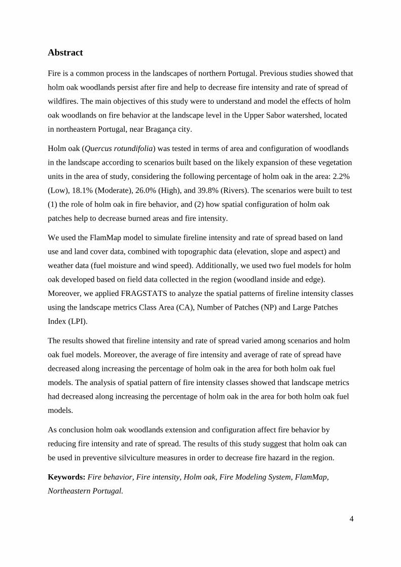
Abstract
Fire is a common process in the landscapes of northern Portugal. Previous studies showed that
holm oak woodlands persist after fire and help to decrease fire intensity and rate of spread of
wildfires. The main objectives of this study were to understand and model the effects of holm
oak woodlands on fire behavior at the landscape level in the Upper Sabor watershed, located
in northeastern Portugal, near Bragança city.
Holm oak (Quercus rotundifolia) was tested in terms of area and configuration of woodlands
in the landscape according to scenarios built based on the likely expansion of these vegetation
units in the area of study, considering the following percentage of holm oak in the area: 2.2%
(Low), 18.1% (Moderate), 26.0% (High), and 39.8% (Rivers). The scenarios were built to test
(1) the role of holm oak in fire behavior, and (2) how spatial configuration of holm oak
patches help to decrease burned areas and fire intensity.
We used the FlamMap model to simulate fireline intensity and rate of spread based on land
use and land cover data, combined with topographic data (elevation, slope and aspect) and
weather data (fuel moisture and wind speed). Additionally, we used two fuel models for holm
oak developed based on field data collected in the region (woodland inside and edge).
Moreover, we applied FRAGSTATS to analyze the spatial patterns of fireline intensity classes
using the landscape metrics Class Area (CA), Number of Patches (NP) and Large Patches
Index (LPI).
The results showed that fireline intensity and rate of spread varied among scenarios and holm
oak fuel models. Moreover, the average of fire intensity and average of rate of spread have
decreased along increasing the percentage of holm oak in the area for both holm oak fuel
models. The analysis of spatial pattern of fire intensity classes showed that landscape metrics
had decreased along increasing the percentage of holm oak in the area for both holm oak fuel
models.
As conclusion holm oak woodlands extension and configuration affect fire behavior by
reducing fire intensity and rate of spread. The results of this study suggest that holm oak can
be used in preventive silviculture measures in order to decrease fire hazard in the region.
Keywords: Fire behavior, Fire intensity, Holm oak, Fire Modeling System, FlamMap,
Northeastern Portugal.
5
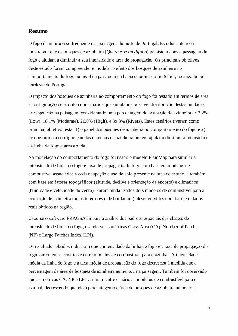
Resumo
O fogo é um processo frequente nas paisagens do norte de Portugal. Estudos anteriores
mostraram que os bosques de azinheira (Quercus rotundifolia) persistem após a passagem do
fogo e ajudam a diminuir a sua intensidade e taxa de propagação. Os principais objetivos
deste estudo foram compreender e modelar o efeito dos bosques de azinheira no
comportamento do fogo ao nível da paisagem da bacia superior do rio Sabor, localizado no
nordeste de Portugal.
O impacto dos bosques de azinheira no comportamento do fogo foi testado em termos de área
e configuração de acordo com cenários que simulam a possível distribuição destas unidades
de vegetação na paisagem, considerando uma percentagem de ocupação da azinheira de 2.2%
(Low), 18.1% (Moderate), 26.0% (High), e 39.8% (Rivers). Estes cenários tiveram como
principal objetivo testar 1) o papel dos bosques de azinheira no comportamento do fogo e 2)
de que forma a configuração das manchas de azinheira podem ajudar a diminuir a intensidade
da linha de fogo e área ardida.
Na modelação do comportamento do fogo foi usado o modelo FlamMap para simular a
intensidade de linha do fogo e taxa de propagação do fogo com base em modelos de
combustível associados a cada ocupação e uso do solo presente na área de estudo, e também
com base em fatores topográficos (altitude, declive e orientação da encosta) e climáticos
(humidade e velocidade do vento). Foram ainda usados dois modelos de combustível para a
ocupação de azinheira (áreas interiores e de bordadura), desenvolvidos com base em dados
reais obtidos na região.
Usou-se o software FRAGSATS para a análise dos padrões espaciais das classes de
intensidade de linha do fogo, usando-se as métricas Class Area (CA), Number of Patches
(NP) e Large Patches Index (LPI).
Os resultados obtidos indicaram que a intensidade da linha de fogo e a taxa de propagação do
fogo variou entre cenários e entre modelos de combustível para o azinhal. A intensidade
média da linha de fogo e a taxa média de propagação do fogo decresceu à medida que a
percentagem de área de bosques de azinheira aumentou na paisagem. Também foi observado
que as métricas CA, NP e LPI variaram entre cenários e modelos de combustível para o
azinhal, decrescendo quando a percentagem de área de bosques de azinheira aumentou.

6
Este estudo permitiu concluir que a variação da percentagem de ocupação e configuração
espacial dos bosques de azinheira influenciam o comportamento do fogo, reduzindo, em
termos médios, a intensidade da linha de fogo e a taxa de propagação, sugerindo que os
bosques de azinhal podem ser usados como medidas silvícolas preventivas para diminuir o
risco de incêndio nesta região.
7
Index Acknowledgements ................................................................................................................................3
Abstract ......................................................................................................................................4
Resumo …...................................................................................................................................5
1. Introduction .......................................................................................................................... 10
2. Literature Review ................................................................................................................. 12
2.1. Fire behavior and landscape structure ........................................................................... 12
2.2- Fire behavior modeling ................................................................................................. 15
3. Methods ................................................................................................................................ 17
3.1. Study area ...................................................................................................................... 17
3.2 Fire modeling and simulations ....................................................................................... 21
3.2.1 FlamMap .................................................................................................................. 21
3.2.2 Experimental design ................................................................................................. 22
3.2.3 Scenarios .................................................................................................................. 22
3.3 Data ................................................................................................................................. 25
3.3.1 Land use and weather ............................................................................................... 25
3.3.2 Terrain ...................................................................................................................... 25
3.3.3 Fuel models .............................................................................................................. 26
3.3.4. Canopy Cover ......................................................................................................... 30
3.4 Analysis .......................................................................................................................... 31
4. Results .................................................................................................................................. 33
5. Discussion ............................................................................................................................ 43
6. Implications to management ................................................................................................ 47
7. Conclusion ............................................................................................................................ 49
8. References ............................................................................................................................ 50
8
List of Figures
Figure 1. Location of the study area, the Sabor River’s upper basin, in Northeastern Portugal.
.................................................................................................................................................. 17
Figure 2.Spatial distribution of the five major LULC classes, with forests subdived in
subclasses in the Sabor River’s upper basin, Northeastern Portugal Data source: COS2007
(Caetano et al., 2009)/IGP). ..................................................................................................... 18
Figure 3. Spatial distribution of holm oak woodlands in the Sabor River’s upper basin. ... 19
Figure 4. Holm oak forest (Quercus rotundifolia). Photo by Azevedo João ............................ 20
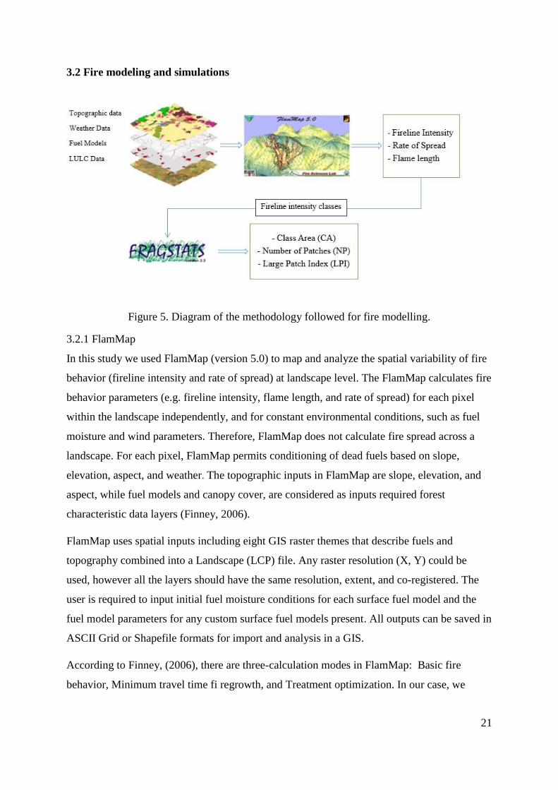
Figure 5. Diagram of the methodology followed for fire modelling. ...................................... 21
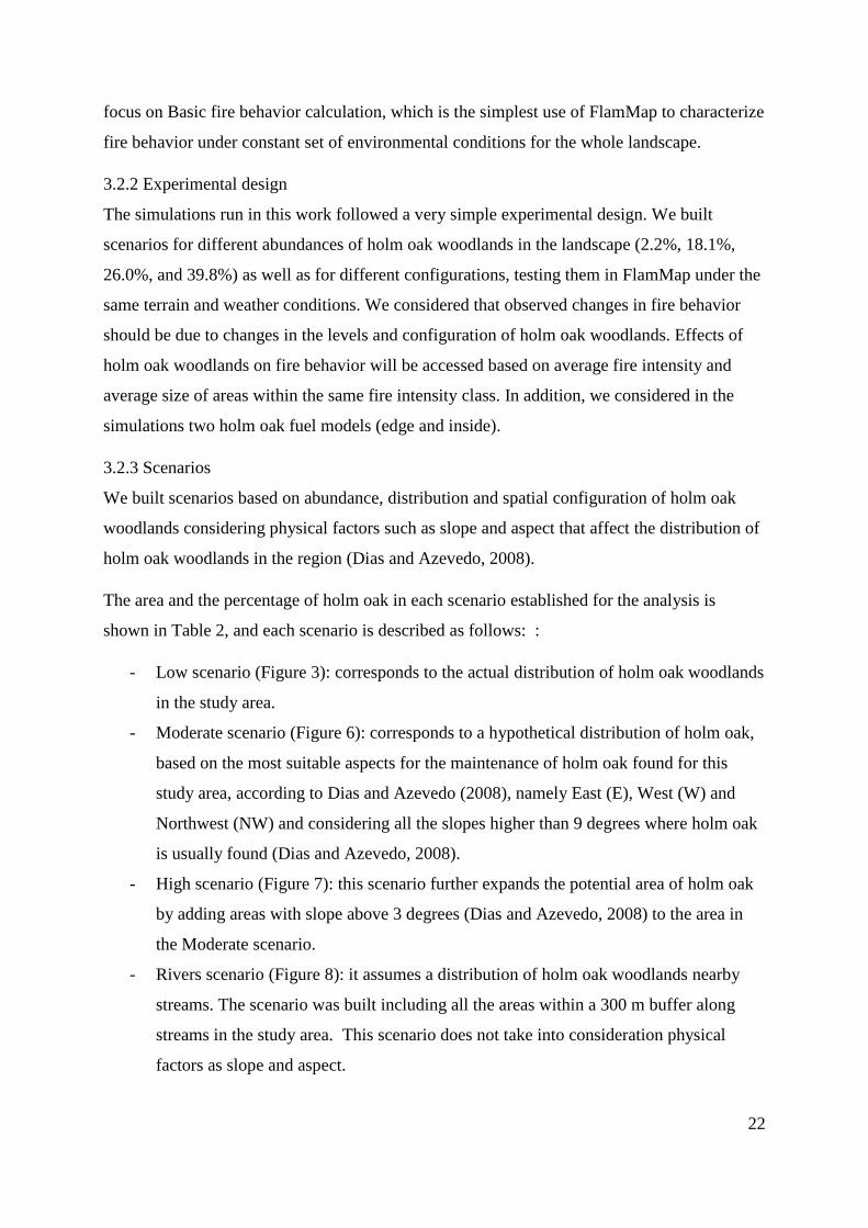
Figure 6. Holm oak distribution in the Sabor river's upper basin according to the Moderate
scenario. .................................................................................................................................... 23
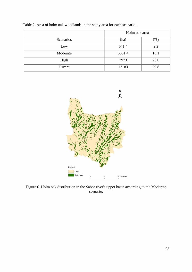
Figure 7. Holm oak distribution in the Sabor River’s upper basin according to the High
scenario. .................................................................................................................................... 24
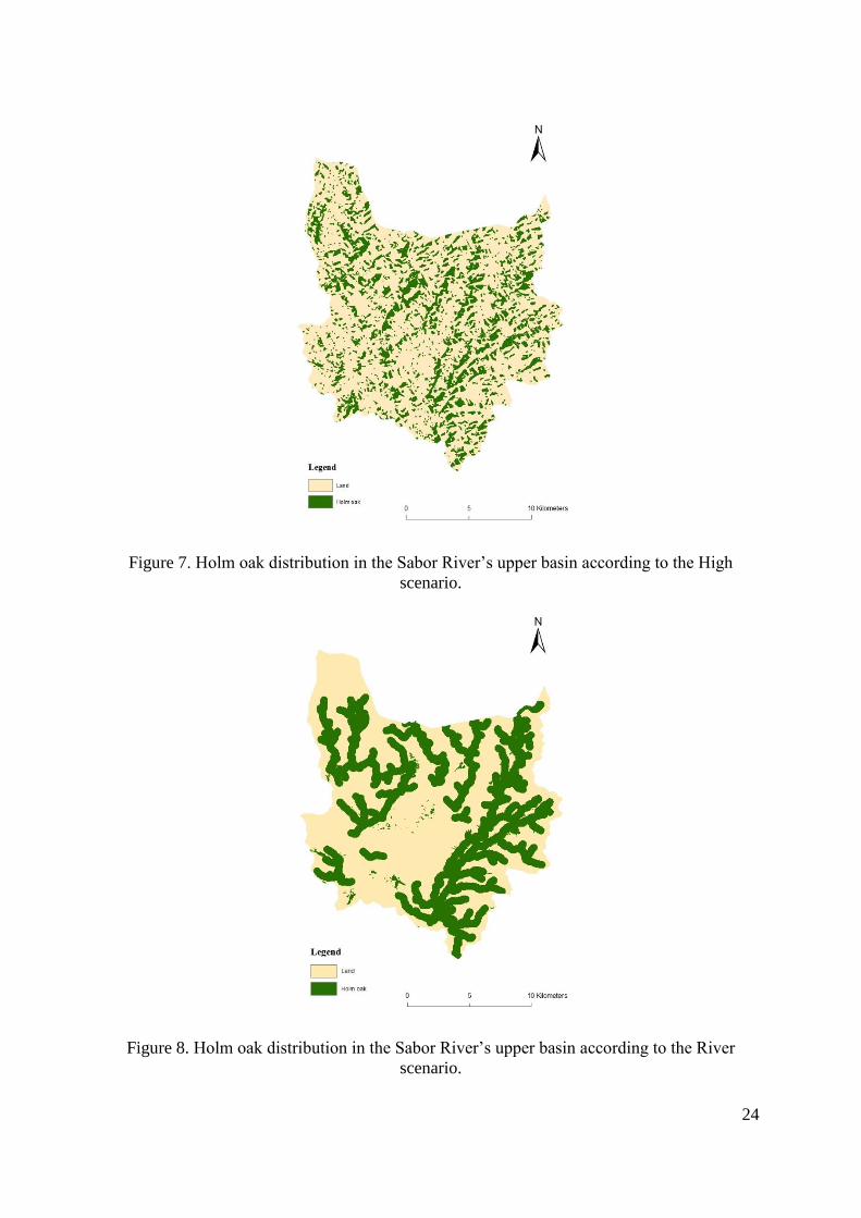
Figure 8. Holm oak distribution in the Sabor River’s upper basin according to the River
scenario. .................................................................................................................................... 24
Figure 9. Sampling procedure: placement of transects across edges and schematic of the
sampling transects and points (from Azevedo et al., (2013)) ................................................... 29
Figure 10. Custom fuel model format as an (.FMD) file for both Holm oak fuel models (inside
and edge), created with FARSITE ........................................................................................... 30
Figure 11. Mean value of fire intensity (kW/m) in terms of scenarios and holm oak fuel
models. ..................................................................................................................................... 34
Figure 12. Mean value of rate of spread (m/min) in terms of scenarios and holm oak fuel
models. ..................................................................................................................................... 34
Figure 13. Maps of fire intensity classes for Low, Moderate, High and River scenario showing
how fire intensity and fire behavior is changing over scenarios, created by ArcMap. ............ 35
Figure 14. Area class (ha) of fire line intensity in each scenario for both fuel holm oak models
(inside and edge). ..................................................................................................................... 36
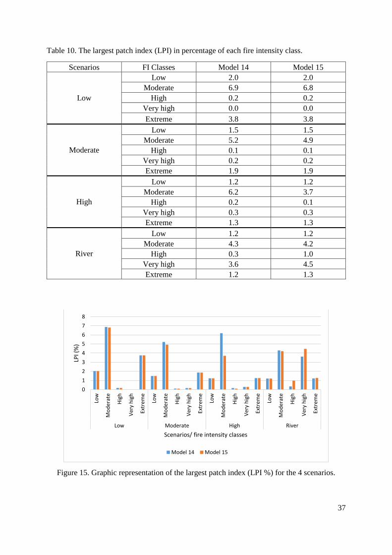
Figure 15. Graphic representation of the largest patch index (LPI %) for the 4 scenarios. ..... 37
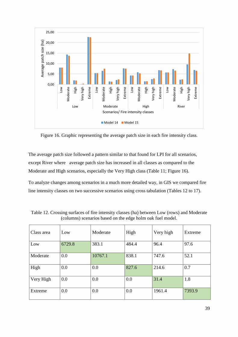
Figure 16. Graphic representing the average patch size in each fire intensity class. ............... 39
Figure 17. Comparison between holm oak woodlands and fire intensity classes, Holm oak
woodlands correspond to high and very high classes............................................................... 44
Figure 18. Maps showing that fuel model 4 areas are occupied by the areas of Extreme fire
intensity class. .......................................................................................................................... 45
9
List of Tables
Table 1. Area of Land use/ Land cover in (ha) and (%) in the Sabor River’s upper basin,
Northeastern Portugal. Calculated in GIS from COS2007 data (Caetano et al., 2009)/IGP) .. 19
Table 2. Area of holm oak woodlands in the study area for each scenario. ............................. 22
Table 3. Fuel model classification, distribution and correspondence with Land use and Land
cover classes in the Upper Sabor watershed. Adopted from Azevedo et al., 2011 .................. 26
Table 4. Custom fuel models Format parameters. ................................................................... 28
Table 5. Canopy cover values used for different forest types in the fire behavior simulations
source: Table14.2 Azevedo et al., (2011). ................................................................................ 31
Table 6. Fire line intensity classes adopted from Alexander and Lanoville (1989). ................ 31
Table 7. Mean fire intensity (kW/m) for each scenario in both holm oak fuel models. .......... 33
Table 8. Mean rate of spread (m/min) for each scenario in both holm oak fuel models.......... 33
Table 9. Class area (ha) of fire line intensity for scenarios Low, Moderate, High and River.. 36
Table 10. The largest patch index (LPI) in percentage of each fire intensity class.................. 37
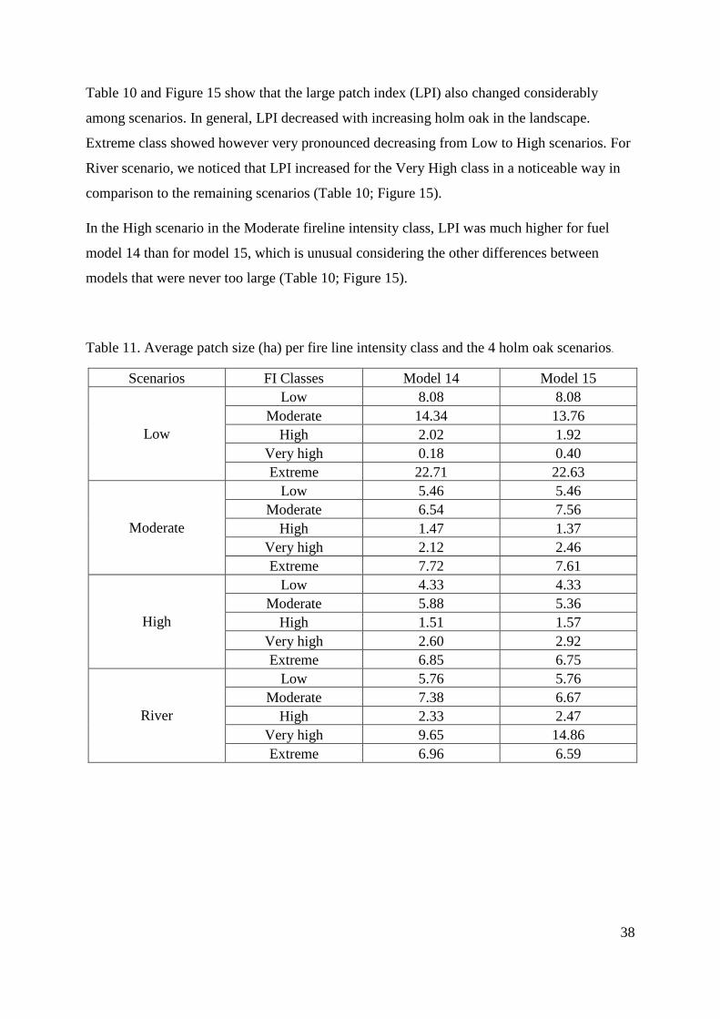
Table 11. Average patch size (ha) per fire line intensity class and the 4 holm oak scenarios. 38
Table 12. Crossing surfaces of fire intensity classes (ha) between Low (rows) and Moderate
(columns) scenarios based on the edge holm oak fuel model. ................................................. 39
Table 13. Crossing surfaces of fire intensity classes (ha) between Low (rows) and Moderate
(columns) scenarios based on the inside holm oak model. ...................................................... 40
Table 14.Crossing surfaces of fire intensity classes (ha) between Moderate (rows) and High
(columns) scenarios based on the edge holm oak model. ........................................................ 40
Table 15. Crossing surfaces of fire intensity classes (ha) between Moderate (rows) and High
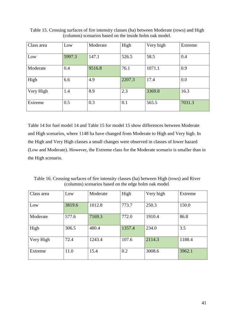
(columns) scenarios based on the inside holm oak model. ...................................................... 41
Table 16. Crossing surfaces of fire intensity classes (ha) between High (rows) and River
(columns) scenarios based on the edge holm oak model. ........................................................ 41
Table 17. Crossing surfaces of fire intensity classes (ha) between High (rows) and River
(columns) scenarios based on the inside holm oak model. ...................................................... 42
Table 18. Total fuel load dead and live (tons/ ha) for fuel models represented in the landscape
of study; values adapted from Anderson (1982). ..................................................................... 45
10
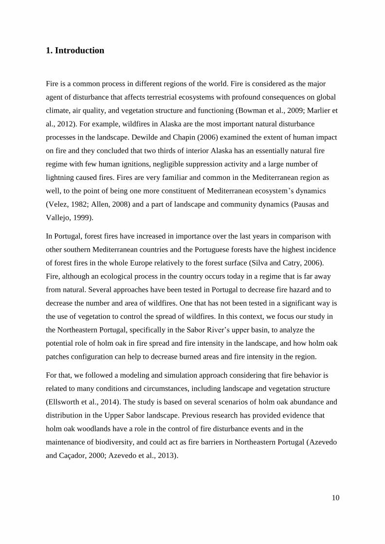
1. Introduction
Fire is a common process in different regions of the world. Fire is considered as the major
agent of disturbance that affects terrestrial ecosystems with profound consequences on global
climate, air quality, and vegetation structure and functioning (Bowman et al., 2009; Marlier et
al., 2012). For example, wildfires in Alaska are the most important natural disturbance
processes in the landscape. Dewilde and Chapin (2006) examined the extent of human impact
on fire and they concluded that two thirds of interior Alaska has an essentially natural fire
regime with few human ignitions, negligible suppression activity and a large number of
lightning caused fires. Fires are very familiar and common in the Mediterranean region as
well, to the point of being one more constituent of Mediterranean ecosystem’s dynamics
(Velez, 1982; Allen, 2008) and a part of landscape and community dynamics (Pausas and
Vallejo, 1999).
In Portugal, forest fires have increased in importance over the last years in comparison with
other southern Mediterranean countries and the Portuguese forests have the highest incidence
of forest fires in the whole Europe relatively to the forest surface (Silva and Catry, 2006).
Fire, although an ecological process in the country occurs today in a regime that is far away
from natural. Several approaches have been tested in Portugal to decrease fire hazard and to
decrease the number and area of wildfires. One that has not been tested in a significant way is
the use of vegetation to control the spread of wildfires. In this context, we focus our study in
the Northeastern Portugal, specifically in the Sabor River’s upper basin, to analyze the
potential role of holm oak in fire spread and fire intensity in the landscape, and how holm oak
patches configuration can help to decrease burned areas and fire intensity in the region.
For that, we followed a modeling and simulation approach considering that fire behavior is
related to many conditions and circumstances, including landscape and vegetation structure
(Ellsworth et al., 2014). The study is based on several scenarios of holm oak abundance and
distribution in the Upper Sabor landscape. Previous research has provided evidence that
holm oak woodlands have a role in the control of fire disturbance events and in the
maintenance of biodiversity, and could act as fire barriers in Northeastern Portugal (Azevedo
and Caçador, 2000; Azevedo et al., 2013).

11
In this work, we used knowledge and fuel models from previous research to analyze how fire
behavior and burned areas change with changing holm oak scenarios, and based on our results
we understand better the role of holm oak woodlands in fire behavior.
12
2. Literature Review
2.1. Fire behavior and landscape structure
Wildfires are a very common type of disturbance in different parts of the world, occurring
from a large percentage of natural origin especially lightning (Alexander et al., 1998) or
human causes like cigarettes and sparks from cutting (Plucinski, 2014). For example, in
Alaska, fires are the major natural agent of disturbance (Dewilde and Chapin, 2006), while in
Mediterranean regions, fires are considered as an integral constituent of the dynamics of
landscapes (Velez, 1982; Allen, 2008). In European Mediterranean areas, the number of fires
and surface burned have increased recently (Pausas and Vallejo, 1999). This increase is
mainly due to two factors: land use changes derived from rural depopulation, which increases
land abandonment and fuel accumulation, and climatic warming, an increase in air
temperature and reduction in summer rainfall, humidity and fuel moisture (Pausas and
Vallejo, 1999). In Portugal, forest are characterized by the highest incidence of forest fires in
the whole of Europe (Silva and Catry, 2006). Comparing the average relationship between
total burned area and forest surface in the south of Europe, Portugal takes the first place. In
terms of distribution, forest fires are mostly concentrated in the northern part of the country
(Silva and Catry, 2006).
Fire behavior is influenced by the interaction of three main components: fuel models or
vegetation (Agee, 1996; Nunes et al., 2005; Perera et al., 2009; Viedma et al., 2009),
topography and weather (Agee, 1996; Alexander et al., 2006). They represent the “fire
behavior triangle”, but the fuel component is the most related to the landscape structure and
the only one that we can control (Agee, 1996).
The description of fire behavior can be made using many parameters as fire length, rate of
spread, and fire intensity which is one of the most useful metrics to understand fire behavior
in forests (Keeley, 2009). According to Alexander (1982), fire intensity can be defined as a
valid measure of forest fires that represents the energy output rate per unit length of fire front
and it is the only physical attribute of fire. Moreover, fire intensity can be defined as the
product of net heat of combustion, representing also the quantity of fuel consumed in the
active combustion zone, and the spreading fire’s linear rate of advance (Alexander, 1982).
Fire intensity is a concept that provides a quantitative basis for fire description, useful in
evaluating the impact of fire on forest ecosystems.
13
In recent papers dealing with post-fire studies (e.g. Simard 1991; Parsons 2003; Jain et al.,
2004; Lentile et al., 2006), there has been a disturbing number that have acknowledged
problems in terminology associated with fire intensity and fire severity. According to Keeley
(2009), the problem with fire intensity is that is sometimes used incorrectly to describe fire
effects when actually it is justifiably restricted to measures of energy output. Lentile et al.,
(2006) suggested replacing fire intensity and fire severity with new categories such as “active
fire characteristics” and “post-fire effects”. Fireline intensity and fire severity are two
different parameters. The first one is a physical parameter referring to energy release rate per
unit length of fireline (Agee, 1996; Keely, 2009) which is related to flame length, and it can
be determined from rate of spread of the fire. The second parameter, fire severity, is
considered as an ecological parameter that measures the effects of fire (Agee, 1996). The fire
line intensity and potential fire severity are both related to fuels surface.
In general, fires are selective. Depending on the land cover type where fire occurs, the
incidence is higher (preferred) or lower (avoided) in a selectivity process that is expressed by
the number of fires expected in a given land cover and by the mean surface area each fire will
burn (Bajocco and Ricotta, 2008). Fire risk assessment at the landscape scale indicates that
risk of wildfires is closely related to land cover (Bajocco and Ricotta, 2008). There is a close
relationship between the timing of fire occurrence and land cover, that is mainly controlled by
two complementary processes: climatic factors, acting indirectly on the timing of wildfires,
determining the spatial distribution of land use types as well, and human population and
human pressure that directly influence fire ignition (Bajocco et al., 2010).
According to Azevedo et al., (2011) changes caused by human abandonment affect the
structure of landscapes and their composition in Northeastern Portugal, which can lead to
changes in fire behavior, increasing fireline intensity and average burned area, enhancing the
landscape conditions for the occurrence of intense fire events over time.
Ellsworth et al., (2014) determined how potential fire behavior could differ between land
cover types. These authors tested how land cover changes along two grassland/forest ecotones
in Hawaii would influence fire behavior, analyzing repeated fires during a time period of 61
years using the BehavePlus fire modeling program. Their results demonstrated that when
forests are converted to grasslands fire intensity increases significantly.
14
The impact of fire on landscape pattern is variable depending on the regions. This variability
is due to the different regeneration abilities of main land cover types, topographic constraints
and the fire history of each region (Viedma, 2008).
One of the most noticeable characteristics of the Portuguese forest is the fact that it has the
highest surface of cork oak stands in the whole Europe. The cork in these trees is very
resistant to fire which help somehow to mitigate the effects of wildfires in cork oak stands,
although fire causes a high risk of tree decay and other accumulated stress like bark stripping
(Silva and Catry, 2006).
Catry et al., (2010) studied the effects of fire on woody species analyzing 1040 burned trees
from 11 different species in mixed forests of central Portugal. These authors found that almost
all broadleaves trees survived but most coniferous died. Despite the low mortality of
broadleaves, most of them were top-killed and regenerated only from basal resprouts.
Quercus suber showed a strong post-fire crown resprouting and it was found to be the most
resilient of the species studied (Catry et al., 2010). Fires damaged also soils because during
burning they lose nutrients and after burning the risk of erosion increases (Pausas and Vallejo,
1999).
Catry et al., (2014) studied the impacts of wildfires in cork oak patterns in the Mediterranean
basin and its relation with post-fire disturbances. They observed an apparent outbreak of bark
beetles in 47% of burned trees, which was related to tree diameter, fire severity and pre-fire
trunk wounded surface, while in unburned trees there was no evidence of bark beetles attacks.
In the Mediterranean basin, species such as Quercus ilex and Pinus halepensis are common
trees and they can regenerate reliably after fire. Quercus ilex resprouts vigorously after
disturbances, while Pinus halepensis colonize disturbed areas by effective seedlings
recruitment. The monospecific forests of Pinus or Quercus have a high probability of
remaining in their original composition after fire, while mixed forest of the two species was
quite low (Brancano et al., 2005). For both species, plots that changed to another forest type
are mainly those that burned more severely, and in the mixed forests, low fire severities
involve high probabilities of change to monospecific forests (Brancano et al., 2005).
15
Quercus ilex plays an important role in Western Mediterranean ecosystems, but in the Eastern
Mediterranean part, it is poorly developed and often replaced by Quercus calliprinos (Barbero
et al., 1992).
Holm oak woodlands have an important role in landscape patterns and processes, and they
participate in the control of perturbation events and in the maintenance of biodiversity
(Azevedo et al., 2013)
Observations and studies in the Northeast of Portugal suggest that holm oak woodlands are
resistant to fire and this resistance is due to modifications in fire behavior at the shrublands-
woodland interface level (Azevedo and Caçador, 2000; Dias and Azevedo, 2008; Azevedo et
al., 2013). A high variation was observed in fire behavior along the exterior-interior gradients
in holm oak woodland edges, which are related to variations in the structure of the vegetation
(Azevedo et al., 2013). As a conclusion, the study indicated that wildfire spread and intensity
decrease when in contact with holm oak woodlands which can lead to their natural extinction
(Azevedo et al., 2013).
2.2- Fire behavior modeling
Simulation is an important tool to predict fire behavior and effects for a wide diversity
(Keane et al., 2011). Fire simulation modelling has been concentrated on describing the
growth and intensity of fires, because more than 90% of all wildland fires are confined to the
surface fire stage where fire control forces can be effective (Rothermel, 1982).
Deterministic and probabilistic geospatial fire behavior analyses are conducted with different
modelling systems such as BEHAVE FARSITE, FlamMap, FSPro, WindWizard, and
FIRETEC to simulate fire behavior and predict fire growth process (Hollingsworth et al.,
2012; Forghani et al., 2014).
Andrews (1986), described BEHAVE as a fire prediction and fuel modelling system. The
BEHAVE is of limited use for predicting fire effects, but it is a flexible system that can be
adapted to different specific wildland fire management needs. According to Andrews (2013),
among the most widely used systems for wildland fire prediction there is the BehavePlus fire
modelling system. It is successor to BEHAVE, which was developed in 1977. The
BehavePlus is designed to use in several tasks including wildfire behavior, prediction
prescribed fire planning, fire investigation fuel hazard assessment, fire model understanding.

16
This fire modelling system is based on mathematical models for fire behavior, fire effect and
fire environment.
Finney (2006) gives an overview of FlamMap fire modeling capabilities and describe this fire
behavior modeling system. According to him, the FlamMap is designed to examine spatial
variability in fire behavior; it may also be used for several fires management activities, and
for pre and post fuel treatment evaluation.
FARSITE (Finney, 2004) is a fire growth simulation modeling system, used for short period
of time, in order to project the fire growth of ongoing fires and hypothetical fires for planning.
It requires an eight spatial data layers for a comprehensive evaluation of surface and crown
fire behavior. FARSITE spreads fire across a landscape using the fire behavior routines found
in the one-dimensional fire model BEHAVE (Andrews 1986; Rothermal 1972).
Duncan et al., (2015) conducted a study to compare fuels reduction and patch mosaic fire
regimes for reducing fire hazard, adapting a spatial modelling approach using a computer
simulation with the FARSITE fire model. In the same context, Pimont et al., (2016) presented
a spatially-explicit-fuel-modelling system, fuel manager, using a physics based model:
FIRETEC to model fuels, vegetation growth, fire behavior and fire effects.
Fire behavior modelling could be done using mathematical models to relate physical and
chemical properties of fuel arrays to specific fire behavior (Albini, 1976). One of those
mathematical models is nomographs, used to describe fire behavior by using Rothermel’s
equations (Rothermel, 1983) and some stylized fuel models to draw a set of graphs (Albini,
1976).
17
3. Methods
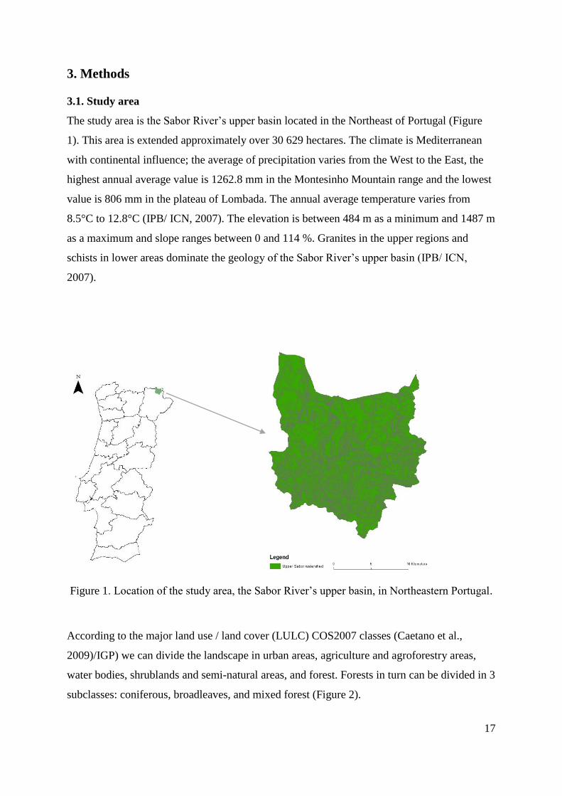
3.1. Study area
The study area is the Sabor River’s upper basin located in the Northeast of Portugal (Figure
1). This area is extended approximately over 30 629 hectares. The climate is Mediterranean
with continental influence; the average of precipitation varies from the West to the East, the
highest annual average value is 1262.8 mm in the Montesinho Mountain range and the lowest
value is 806 mm in the plateau of Lombada. The annual average temperature varies from
8.5°C to 12.8°C (IPB/ ICN, 2007). The elevation is between 484 m as a minimum and 1487 m
as a maximum and slope ranges between 0 and 114 %. Granites in the upper regions and
schists in lower areas dominate the geology of the Sabor River’s upper basin (IPB/ ICN,
2007).
Figure 1. Location of the study area, the Sabor River’s upper basin, in Northeastern Portugal.
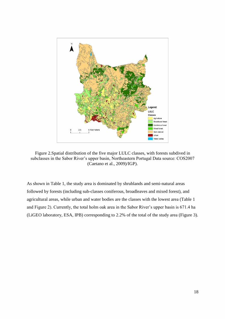
According to the major land use / land cover (LULC) COS2007 classes (Caetano et al.,
2009)/IGP) we can divide the landscape in urban areas, agriculture and agroforestry areas,
water bodies, shrublands and semi-natural areas, and forest. Forests in turn can be divided in 3
subclasses: coniferous, broadleaves, and mixed forest (Figure 2).
18
Figure 2.Spatial distribution of the five major LULC classes, with forests subdived in
subclasses in the Sabor River’s upper basin, Northeastern Portugal Data source: COS2007
(Caetano et al., 2009)/IGP).
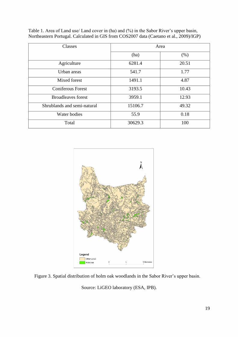
As shown in Table 1, the study area is dominated by shrublands and semi-natural areas
followed by forests (including sub-classes coniferous, broadleaves and mixed forest), and
agricultural areas, while urban and water bodies are the classes with the lowest area (Table 1
and Figure 2). Currently, the total holm oak area in the Sabor River’s upper basin is 671.4 ha
(LiGEO laboratory, ESA, IPB) corresponding to 2.2% of the total of the study area (Figure 3).
19
Table 1. Area of Land use/ Land cover in (ha) and (%) in the Sabor River’s upper basin,
Northeastern Portugal. Calculated in GIS from COS2007 data (Caetano et al., 2009)/IGP)
Figure 3. Spatial distribution of holm oak woodlands in the Sabor River’s upper basin.
Source: LiGEO laboratory (ESA, IPB).
Classes Area
(ha) (%)
Agriculture 6281.4 20.51
Urban areas 541.7 1.77
Mixed forest 1491.1 4.87
Coniferous Forest 3193.5 10.43
Broadleaves forest 3959.1 12.93
Shrublands and semi-natural 15106.7 49.32
Water bodies 55.9 0.18
Total 30629.3 100
20
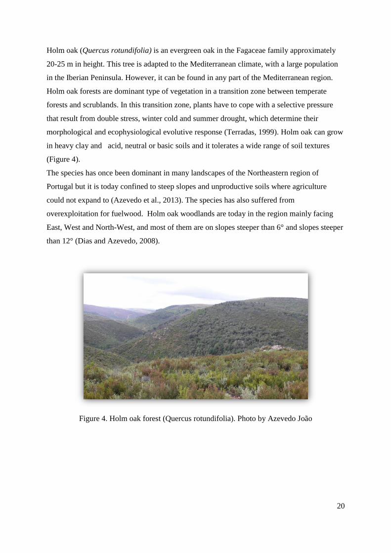
Holm oak (Quercus rotundifolia) is an evergreen oak in the Fagaceae family approximately
20-25 m in height. This tree is adapted to the Mediterranean climate, with a large population
in the Iberian Peninsula. However, it can be found in any part of the Mediterranean region.
Holm oak forests are dominant type of vegetation in a transition zone between temperate
forests and scrublands. In this transition zone, plants have to cope with a selective pressure
that result from double stress, winter cold and summer drought, which determine their
morphological and ecophysiological evolutive response (Terradas, 1999). Holm oak can grow
in heavy clay and acid, neutral or basic soils and it tolerates a wide range of soil textures
(Figure 4).
The species has once been dominant in many landscapes of the Northeastern region of
Portugal but it is today confined to steep slopes and unproductive soils where agriculture
could not expand to (Azevedo et al., 2013). The species has also suffered from
overexploitation for fuelwood. Holm oak woodlands are today in the region mainly facing
East, West and North-West, and most of them are on slopes steeper than 6° and slopes steeper
than 12° (Dias and Azevedo, 2008).
Figure 4. Holm oak forest (Quercus rotundifolia). Photo by Azevedo João
21
3.2 Fire modeling and simulations
Figure 5. Diagram of the methodology followed for fire modelling.
3.2.1 FlamMap
In this study we used FlamMap (version 5.0) to map and analyze the spatial variability of fire
behavior (fireline intensity and rate of spread) at landscape level. The FlamMap calculates fire
behavior parameters (e.g. fireline intensity, flame length, and rate of spread) for each pixel
within the landscape independently, and for constant environmental conditions, such as fuel
moisture and wind parameters. Therefore, FlamMap does not calculate fire spread across a
landscape. For each pixel, FlamMap permits conditioning of dead fuels based on slope,
elevation, aspect, and weather. The topographic inputs in FlamMap are slope, elevation, and
aspect, while fuel models and canopy cover, are considered as inputs required forest
characteristic data layers (Finney, 2006).
FlamMap uses spatial inputs including eight GIS raster themes that describe fuels and
topography combined into a Landscape (LCP) file. Any raster resolution (X, Y) could be
used, however all the layers should have the same resolution, extent, and co-registered. The
user is required to input initial fuel moisture conditions for each surface fuel model and the
fuel model parameters for any custom surface fuel models present. All outputs can be saved in
ASCII Grid or Shapefile formats for import and analysis in a GIS.
According to Finney, (2006), there are three-calculation modes in FlamMap: Basic fire
behavior, Minimum travel time fi regrowth, and Treatment optimization. In our case, we
22
focus on Basic fire behavior calculation, which is the simplest use of FlamMap to characterize
fire behavior under constant set of environmental conditions for the whole landscape.
3.2.2 Experimental design
The simulations run in this work followed a very simple experimental design. We built
scenarios for different abundances of holm oak woodlands in the landscape (2.2%, 18.1%,
26.0%, and 39.8%) as well as for different configurations, testing them in FlamMap under the
same terrain and weather conditions. We considered that observed changes in fire behavior
should be due to changes in the levels and configuration of holm oak woodlands. Effects of
holm oak woodlands on fire behavior will be accessed based on average fire intensity and
average size of areas within the same fire intensity class. In addition, we considered in the
simulations two holm oak fuel models (edge and inside).
3.2.3 Scenarios
We built scenarios based on abundance, distribution and spatial configuration of holm oak
woodlands considering physical factors such as slope and aspect that affect the distribution of
holm oak woodlands in the region (Dias and Azevedo, 2008).
The area and the percentage of holm oak in each scenario established for the analysis is
shown in Table 2, and each scenario is described as follows: :
- Low scenario (Figure 3): corresponds to the actual distribution of holm oak woodlands
in the study area.
- Moderate scenario (Figure 6): corresponds to a hypothetical distribution of holm oak,
based on the most suitable aspects for the maintenance of holm oak found for this
study area, according to Dias and Azevedo (2008), namely East (E), West (W) and
Northwest (NW) and considering all the slopes higher than 9 degrees where holm oak
is usually found (Dias and Azevedo, 2008).
- High scenario (Figure 7): this scenario further expands the potential area of holm oak
by adding areas with slope above 3 degrees (Dias and Azevedo, 2008) to the area in
the Moderate scenario.
- Rivers scenario (Figure 8): it assumes a distribution of holm oak woodlands nearby
streams. The scenario was built including all the areas within a 300 m buffer along
streams in the study area. This scenario does not take into consideration physical
factors as slope and aspect.
23
Table 2. Area of holm oak woodlands in the study area for each scenario.
Holm oak area
Scenarios (ha) (%)
Low 671.4 2.2
Moderate 5551.4 18.1
High 7973 26.0
Rivers 12183 39.8
Figure 6. Holm oak distribution in the Sabor river's upper basin according to the Moderate
scenario.
24
Figure 7. Holm oak distribution in the Sabor River’s upper basin according to the High
scenario.
Figure 8. Holm oak distribution in the Sabor River’s upper basin according to the River
scenario.
25
3.3 Data
The data used in this study are mostly those required as inputs or in the preparation of inputs
for FlamMap, such as weather conditions, elevation, slope, and aspect, fuel models and
canopy cover.
3.3.1 Land use and weather
Spatial land use data were adapted from COS2007 (IGP) except for the distribution of holm
oak woodlands in 2010 that was obtained from the LiGEO laboratory (ESA, IPB).
For the weather conditions (fuel moisture conditions and wind speed) are similar to those in
Azevedo et al., (2011). We adopted the moisture and wind speed conditions fixed for all
surface of the fuel models and all the landscape independently of topography or canopy cover.
The values of moisture are as follows: 1h=4%; 10h=5%; 100h=6%; live woody=70%; live
herbaceous=70%, and are correlated with the extreme summer weather conditions. The wind
speed was assumed to be constant of 25 km/h at 6 meters elevation, and for azimuth degree is
equal to 90° (Barros, et al., 2012). For fire behavior characteristics calculation we assumed an
uphill wind direction (Azevedo et al., 2011).
3.3.2 Terrain
Elevation (DEM) data was obtained from University of Porto website1 (Gonçalves and
Fernandes, 2005; Gonçalves and Morgado, 2008) with a spatial resolution of 25meters, while
slope and aspect were obtained from DEM in GIS environment, using ArcGIS tools.
Aspect: considered as reflection of slope direction faces, measured in degrees (the north is
0°). This theme is used to calculate the combined effect of wind and slope on fire spread by
determining the upslope direction (STARFIRE Project, 2011).
Elevation: is the vertical distance above the sea level, measured in meters (m) or feet (ft),
used to adjust temperature and humidity for changes in elevation (STARFIRE Project, 2011).
Slope: defined as the inclination from the horizontal, it can be measured in percentage or
degrees; in our case the units is percentage. Slope has a double use in FlamMap: computation
1 http://www.fc.up.pt/pessoas/jagoncal/srtm/
26
of slope effects on fire spread and solar radiance at a location (raster cell) (STARFIRE
Project, 2011).
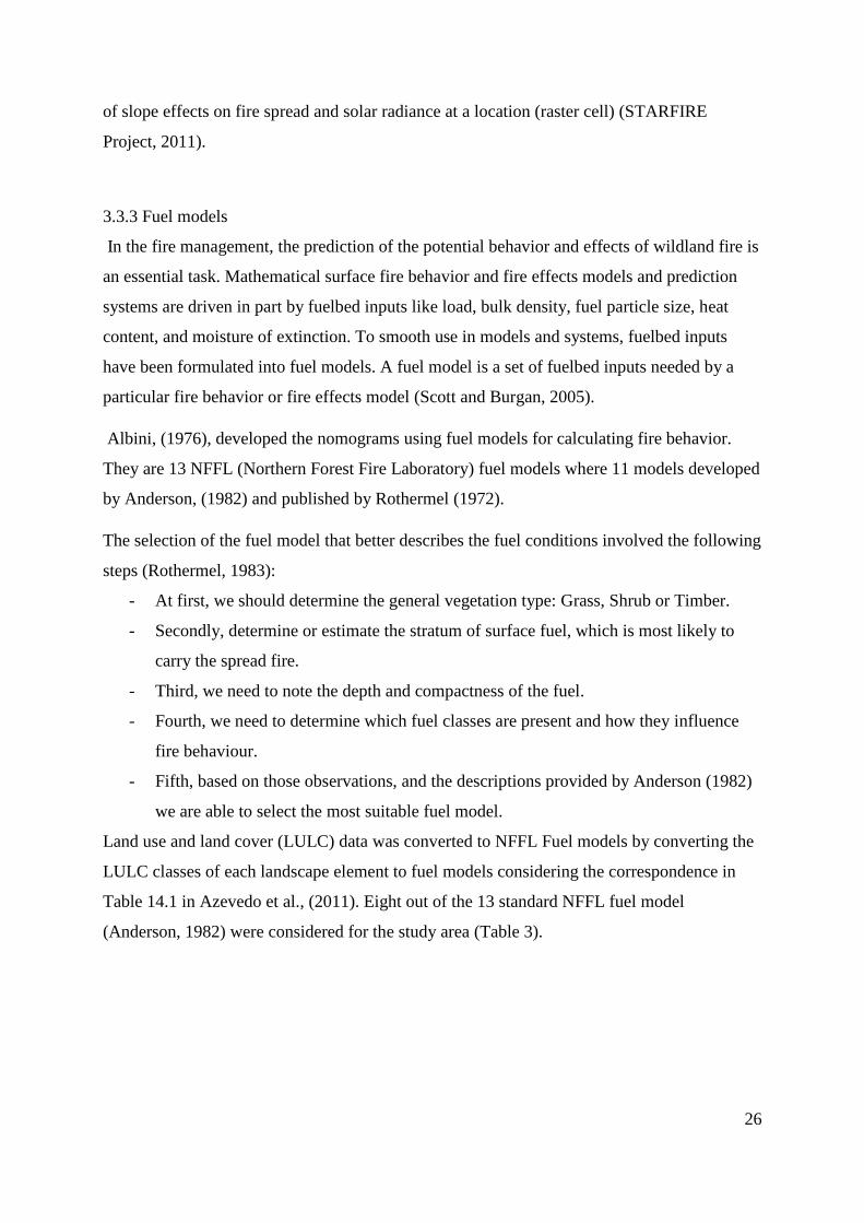
3.3.3 Fuel models
In the fire management, the prediction of the potential behavior and effects of wildland fire is
an essential task. Mathematical surface fire behavior and fire effects models and prediction
systems are driven in part by fuelbed inputs like load, bulk density, fuel particle size, heat
content, and moisture of extinction. To smooth use in models and systems, fuelbed inputs
have been formulated into fuel models. A fuel model is a set of fuelbed inputs needed by a
particular fire behavior or fire effects model (Scott and Burgan, 2005).
Albini, (1976), developed the nomograms using fuel models for calculating fire behavior.
They are 13 NFFL (Northern Forest Fire Laboratory) fuel models where 11 models developed
by Anderson, (1982) and published by Rothermel (1972).
The selection of the fuel model that better describes the fuel conditions involved the following
steps (Rothermel, 1983):
- At first, we should determine the general vegetation type: Grass, Shrub or Timber.
- Secondly, determine or estimate the stratum of surface fuel, which is most likely to
carry the spread fire.
- Third, we need to note the depth and compactness of the fuel.
- Fourth, we need to determine which fuel classes are present and how they influence
fire behaviour.
- Fifth, based on those observations, and the descriptions provided by Anderson (1982)
we are able to select the most suitable fuel model.
Land use and land cover (LULC) data was converted to NFFL Fuel models by converting the
LULC classes of each landscape element to fuel models considering the correspondence in
Table 14.1 in Azevedo et al., (2011). Eight out of the 13 standard NFFL fuel model
(Anderson, 1982) were considered for the study area (Table 3).
27
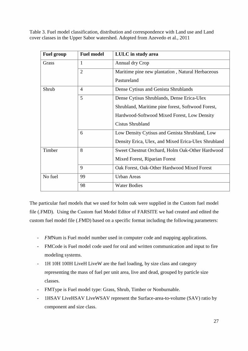
Table 3. Fuel model classification, distribution and correspondence with Land use and Land
cover classes in the Upper Sabor watershed. Adopted from Azevedo et al., 2011
The particular fuel models that we used for holm oak were supplied in the Custom fuel model
file (.FMD). Using the Custom fuel Model Editor of FARSITE we had created and edited the
custom fuel model file (.FMD) based on a specific format including the following parameters:
- FMNum is Fuel model number used in computer code and mapping applications.
- FMCode is Fuel model code used for oral and written communication and input to fire
modeling systems.
- 1H 10H 100H LiveH LiveW are the fuel loading, by size class and category
representing the mass of fuel per unit area, live and dead, grouped by particle size
classes.
- FMType is Fuel model type: Grass, Shrub, Timber or Nonburnable.
- 1HSAV LiveHSAV LiveWSAV represent the Surface-area-to-volume (SAV) ratio by
component and size class.
Fuel group Fuel model LULC in study area
Grass 1 Annual dry Crop
2 Maritime pine new plantation , Natural Herbaceous
Pastureland
Shrub 4 Dense Cytisus and Genista Shrublands
5 Dense Cytisus Shrublands, Dense Erica-Ulex
Shrubland, Maritime pine forest, Softwood Forest,
Hardwood-Softwood Mixed Forest, Low Density
Cistus Shrubland
6 Low Density Cytisus and Genista Shrubland, Low
Density Erica, Ulex, and Mixed Erica-Ulex Shrubland
Timber 8 Sweet Chestnut Orchard, Holm Oak-Other Hardwood
Mixed Forest, Riparian Forest
9 Oak Forest, Oak-Other Hardwood Mixed Forest
No fuel 99 Urban Areas
98 Water Bodies
28
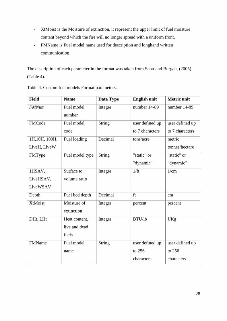
- XtMoist is the Moisture of extinction, it represent the upper limit of fuel moisture
content beyond which the fire will no longer spread with a uniform front.
- FMName is Fuel model name used for description and longhand written
communication.
The description of each parameter in the format was taken from Scott and Burgan, (2005)
(Table 4).
Table 4. Custom fuel models Format parameters.
Field Name Data Type English unit Metric unit
FMNum Fuel model
number
Integer number 14-89 number 14-89
FMCode Fuel model
code
String user defined up
to 7 characters
user defined up
to 7 characters
1H,10H, 100H,
LiveH, LiveW
Fuel loading Decimal tons/acre metric
tonnes/hectare
FMType Fuel model type String "static" or
"dynamic"
"static" or
"dynamic"
1HSAV,
LiveHSAV,
LiveWSAV
Surface to
volume ratio
Integer 1/ft 1/cm
Depth Fuel bed depth Decimal ft cm
XtMoist Moisture of
extinction
Integer percent percent
DHt, LHt Heat content,
live and dead
fuels
Integer BTU/lb J/Kg
FMName Fuel model
name
String user defined up
to 256
characters
user defined up
to 256
characters
29
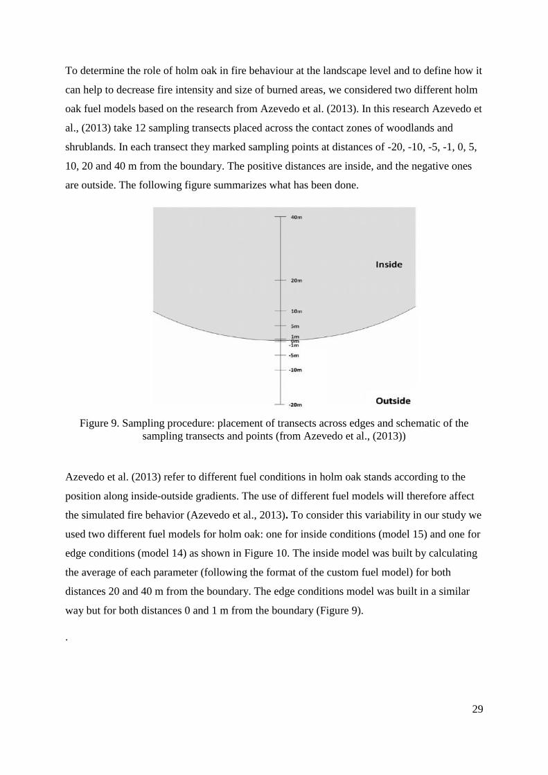
To determine the role of holm oak in fire behaviour at the landscape level and to define how it
can help to decrease fire intensity and size of burned areas, we considered two different holm
oak fuel models based on the research from Azevedo et al. (2013). In this research Azevedo et
al., (2013) take 12 sampling transects placed across the contact zones of woodlands and
shrublands. In each transect they marked sampling points at distances of -20, -10, -5, -1, 0, 5,
10, 20 and 40 m from the boundary. The positive distances are inside, and the negative ones
are outside. The following figure summarizes what has been done.
Figure 9. Sampling procedure: placement of transects across edges and schematic of the
sampling transects and points (from Azevedo et al., (2013))
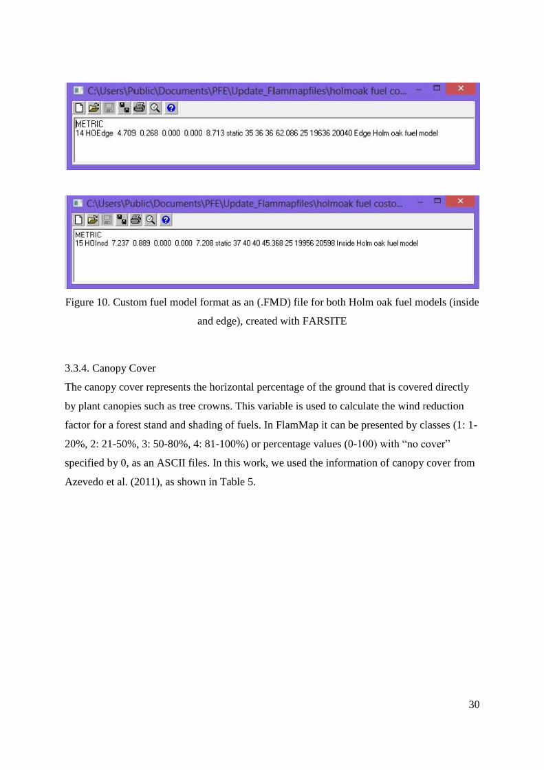
Azevedo et al. (2013) refer to different fuel conditions in holm oak stands according to the
position along inside-outside gradients. The use of different fuel models will therefore affect
the simulated fire behavior (Azevedo et al., 2013). To consider this variability in our study we
used two different fuel models for holm oak: one for inside conditions (model 15) and one for
edge conditions (model 14) as shown in Figure 10. The inside model was built by calculating
the average of each parameter (following the format of the custom fuel model) for both
distances 20 and 40 m from the boundary. The edge conditions model was built in a similar
way but for both distances 0 and 1 m from the boundary (Figure 9).
.
30
Figure 10. Custom fuel model format as an (.FMD) file for both Holm oak fuel models (inside
and edge), created with FARSITE
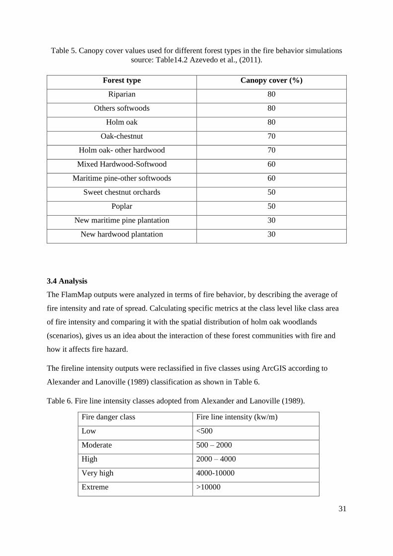
3.3.4. Canopy Cover
The canopy cover represents the horizontal percentage of the ground that is covered directly
by plant canopies such as tree crowns. This variable is used to calculate the wind reduction
factor for a forest stand and shading of fuels. In FlamMap it can be presented by classes (1: 1-
20%, 2: 21-50%, 3: 50-80%, 4: 81-100%) or percentage values (0-100) with “no cover”
specified by 0, as an ASCII files. In this work, we used the information of canopy cover from
Azevedo et al. (2011), as shown in Table 5.
31
Table 5. Canopy cover values used for different forest types in the fire behavior simulations
source: Table14.2 Azevedo et al., (2011).
3.4 Analysis
The FlamMap outputs were analyzed in terms of fire behavior, by describing the average of
fire intensity and rate of spread. Calculating specific metrics at the class level like class area
of fire intensity and comparing it with the spatial distribution of holm oak woodlands
(scenarios), gives us an idea about the interaction of these forest communities with fire and
how it affects fire hazard.
The fireline intensity outputs were reclassified in five classes using ArcGIS according to
Alexander and Lanoville (1989) classification as shown in Table 6.
Table 6. Fire line intensity classes adopted from Alexander and Lanoville (1989).
Fire danger class Fire line intensity (kw/m)
Low <500
Moderate 500 – 2000
High 2000 – 4000
Very high 4000-10000
Extreme >10000
Forest type Canopy cover (%)
Riparian 80
Others softwoods 80
Holm oak 80
Oak-chestnut 70
Holm oak- other hardwood 70
Mixed Hardwood-Softwood 60
Maritime pine-other softwoods 60
Sweet chestnut orchards 50
Poplar 50
New maritime pine plantation 30
New hardwood plantation 30
32
Moreover, the calculating specific metrics at class level, such as class area of fireline
intensity, and comparing it with the spatial distribution of holm oak woodlands (scenarios),
gives us an idea about the interaction of these forest communities with fire and how it affects
fire hazard. Hence, we used the reclassified fireline intensity maps as inputs for FRAGSTATS
(McGarigal and Marks, 1995) to analyze their spatial pattern.
In FRAGSTATS, we selected the following metrics to be calculated at the class level for
each of the classes established based of fireline intensity:
- CA: Class Area (ha), a specific measure of landscape composition; specifically, how
much of the landscape is comprised of a particular class.
- NP: Number of patches corresponding to each class
- LPI: Largest patch index quantifies the percentage of the landscape area comprised by
the largest patch of each class.
After running FRAGSTATS, we obtained outputs with results of the metrics calculations that
will be analyzed to compare scenarios and fuel models
33
4. Results
From simulating fire behavior in the Upper Sabor watershed with FlamMap, we had the first
results for each scenario in the form of maps of the distribution of the variables flame length,
rate of spread and fire line intensity and statistics
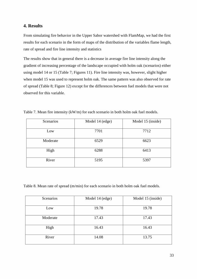
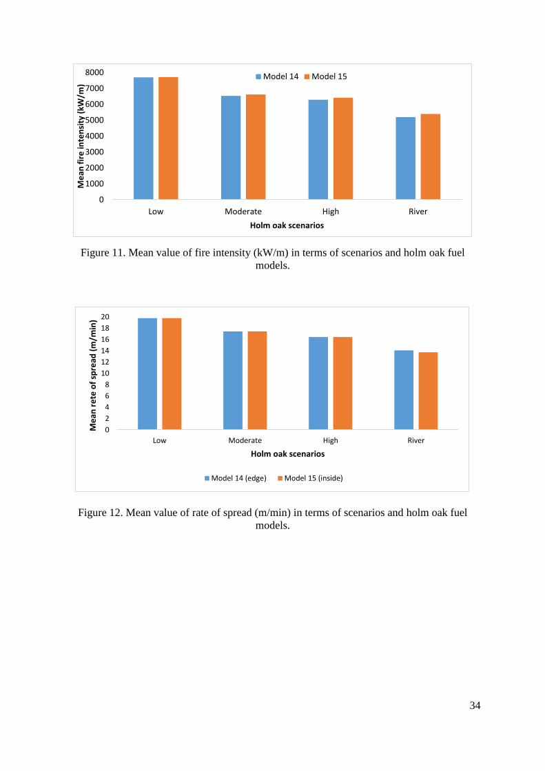
The results show that in general there is a decrease in average fire line intensity along the
gradient of increasing percentage of the landscape occupied with holm oak (scenarios) either
using model 14 or 15 (Table 7; Figures 11). Fire line intensity was, however, slight higher
when model 15 was used to represent holm oak. The same pattern was also observed for rate
of spread (Table 8; Figure 12) except for the differences between fuel models that were not
observed for this variable.
Table 7. Mean fire intensity (kW/m) for each scenario in both holm oak fuel models.
Table 8. Mean rate of spread (m/min) for each scenario in both holm oak fuel models.
Scenarios Model 14 (edge) Model 15 (inside)
Low 7701 7712
Moderate 6529 6623
High 6288 6413
River 5195 5397
Scenarios Model 14 (edge) Model 15 (inside)
Low 19.78 19.78
Moderate 17.43 17.43
High 16.43 16.43
River 14.08 13.75
34
Figure 11. Mean value of fire intensity (kW/m) in terms of scenarios and holm oak fuel
models.
Figure 12. Mean value of rate of spread (m/min) in terms of scenarios and holm oak fuel
models.
0
1000
2000
3000
4000
5000
6000
7000
8000
Low Moderate High River
Me
an f
ire
inte
nsi
ty (
kW/m
)
Holm oak scenarios
Model 14 Model 15
0
2
4
6
8
10
12
14
16
18
20
Low Moderate High River
Me
an r
ete
of
spre
ad (
m/m
in)
Holm oak scenarios
Model 14 (edge) Model 15 (inside)
35
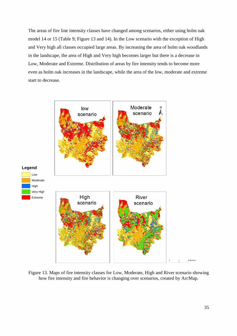
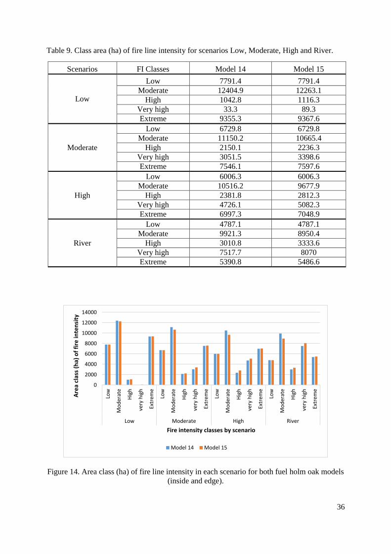
The areas of fire line intensity classes have changed among scenarios, either using holm oak
model 14 or 15 (Table 9; Figure 13 and 14). In the Low scenario with the exception of High
and Very high all classes occupied large areas. By increasing the area of holm oak woodlands
in the landscape, the area of High and Very high becomes larger but there is a decrease in
Low, Moderate and Extreme. Distribution of areas by fire intensity tends to become more
even as holm oak increases in the landscape, while the area of the low, moderate and extreme
start to decrease.
Figure 13. Maps of fire intensity classes for Low, Moderate, High and River scenario showing
how fire intensity and fire behavior is changing over scenarios, created by ArcMap.
Legend
Low
Moderate
High
Very High
Extreme
36
Table 9. Class area (ha) of fire line intensity for scenarios Low, Moderate, High and River.
Scenarios FI Classes Model 14 Model 15
Low
Low 7791.4 7791.4
Moderate 12404.9 12263.1
High 1042.8 1116.3
Very high 33.3 89.3
Extreme 9355.3 9367.6
Moderate
Low 6729.8 6729.8
Moderate 11150.2 10665.4
High 2150.1 2236.3
Very high 3051.5 3398.6
Extreme 7546.1 7597.6
High
Low 6006.3 6006.3
Moderate 10516.2 9677.9
High 2381.8 2812.3
Very high 4726.1 5082.3
Extreme 6997.3 7048.9
River
Low 4787.1 4787.1
Moderate 9921.3 8950.4
High 3010.8 3333.6
Very high 7517.7 8070
Extreme 5390.8 5486.6
Figure 14. Area class (ha) of fire line intensity in each scenario for both fuel holm oak models
(inside and edge).
0
2000
4000
6000
8000
10000
12000
14000
Low
Mo
der
ate
Hig
h
very
hig
h
Extr
em
e
Low
Mo
der
ate
Hig
h
very
hig
h
Extr
em
e
Low
Mo
der
ate
Hig
h
very
hig
h
Extr
em
e
Low
Mo
der
ate
Hig
h
very
hig
h
Extr
em
e
Low Moderate High River
Are
a cl
ass
(ha)
of
fire
inte
nsi
ty
Fire intensity classes by scenario
Model 14 Model 15
37
Table 10. The largest patch index (LPI) in percentage of each fire intensity class.
Scenarios FI Classes Model 14 Model 15
Low
Low 2.0 2.0
Moderate 6.9 6.8
High 0.2 0.2
Very high 0.0 0.0
Extreme 3.8 3.8
Moderate
Low 1.5 1.5
Moderate 5.2 4.9
High 0.1 0.1
Very high 0.2 0.2
Extreme 1.9 1.9
High
Low 1.2 1.2
Moderate 6.2 3.7
High 0.2 0.1
Very high 0.3 0.3
Extreme 1.3 1.3
River
Low 1.2 1.2
Moderate 4.3 4.2
High 0.3 1.0
Very high 3.6 4.5
Extreme 1.2 1.3
Figure 15. Graphic representation of the largest patch index (LPI %) for the 4 scenarios.
0
1
2
3
4
5
6
7
8
Low
Mo
der
ate
Hig
h
Ver
y h
igh
Extr
em
e
Low
Mo
der
ate
Hig
h
Ver
y h
igh
Extr
em
e
Low
Mo
der
ate
Hig
h
Ver
y h
igh
Extr
em
e
Low
Mo
der
ate
Hig
h
Ver
y h
igh
Extr
em
e
Low Moderate High River
LPI (
%)
Scenarios/ fire intensity classes
Model 14 Model 15
38
Table 10 and Figure 15 show that the large patch index (LPI) also changed considerably
among scenarios. In general, LPI decreased with increasing holm oak in the landscape.
Extreme class showed however very pronounced decreasing from Low to High scenarios. For
River scenario, we noticed that LPI increased for the Very High class in a noticeable way in
comparison to the remaining scenarios (Table 10; Figure 15).
In the High scenario in the Moderate fireline intensity class, LPI was much higher for fuel
model 14 than for model 15, which is unusual considering the other differences between
models that were never too large (Table 10; Figure 15).
Table 11. Average patch size (ha) per fire line intensity class and the 4 holm oak scenarios.
Scenarios FI Classes Model 14 Model 15
Low
Low 8.08 8.08
Moderate 14.34 13.76
High 2.02 1.92
Very high 0.18 0.40
Extreme 22.71 22.63
Moderate
Low 5.46 5.46
Moderate 6.54 7.56
High 1.47 1.37
Very high 2.12 2.46
Extreme 7.72 7.61
High
Low 4.33 4.33
Moderate 5.88 5.36
High 1.51 1.57
Very high 2.60 2.92
Extreme 6.85 6.75
River
Low 5.76 5.76
Moderate 7.38 6.67
High 2.33 2.47
Very high 9.65 14.86
Extreme 6.96 6.59
39
Figure 16. Graphic representing the average patch size in each fire intensity class.
The average patch size followed a pattern similar to that found for LPI for all scenarios,
except River where average patch size has increased in all classes as compared to the
Moderate and High scenarios, especially the Very High class (Table 11; Figure 16).
To analyze changes among scenarios in a much more detailed way, in GIS we compared fire
line intensity classes on two successive scenarios using cross tabulation (Tables 12 to 17).
Table 12. Crossing surfaces of fire intensity classes (ha) between Low (rows) and Moderate
(columns) scenarios based on the edge holm oak fuel model.
Class area Low Moderate High Very high Extreme
Low 6729.8 383.1 484.4 96.4 97.6
Moderate 0.0 10767.1 838.1 747.6 52.1
High 0.0 0.0 827.6 214.6 0.7
Very High 0.0 0.0 0.0 31.4 1.8
Extreme 0.0 0.0 0.0 1961.4 7393.9
0,00
5,00
10,00
15,00
20,00
25,00
Low
Mo
der
ate
Hig
h
Ver
y h
igh
Extr
em
e
Low
Mo
der
ate
Hig
h
Ver
y h
igh
Extr
em
e
Low
Mo
der
ate
Hig
h
Ver
y h
igh
Extr
em
e
Low
Mo
der
ate
Hig
h
Ver
y h
igh
Extr
em
e
Low Moderate High River
Ave
rage
pat
ch s
ize
(ha)
Scenarios/ Fire intensity classes
Model 14 Model 15

40
Table 13. Crossing surfaces of fire intensity classes (ha) between Low (rows) and Moderate
(columns) scenarios based on the inside holm oak model.
Major differences in terms of fire hazard between Low and Moderate scenarios were observed
in the moderate fire intensity since more than 1600 ha have changed from Moderate to High
and Very High and, in a much smaller extent, to Extreme. In classes Low and High there
were large areas that moved to classes of higher hazard (Moderate - High and very high).
However, the Extreme class in the Low scenario is 1961 ha smaller than in the Moderate
scenario (Table12 and 13).
Table 14.Crossing surfaces of fire intensity classes (ha) between Moderate (rows) and High
(columns) scenarios based on the edge holm oak model.
Class area Low Moderate High Very high Extreme
Low 6729.8 41.7 723.3 188.8 107.8
Moderate 0.0 10623.7 611.9 955.1 72.4
High 0.0 0.0 901.1 212.6 2.7
Very High 0.0 0.0 0.0 87.4 1.8
Extreme 0.0 0.0 0.0 1954.7 7412.9
Class area Low Moderate High Very high Extreme
Low 5997.3 503.8 172.2 56.1 0.4
Moderate 3.8 9998.3 85.0 1062.5 0.6
High 3.9 6.5 2122.3 17.4 0.0
Very High 0.9 7.3 2.4 3024.6 16.3
Extreme 0.4 0.3 0.0 565.5 6979.9
41
Table 15. Crossing surfaces of fire intensity classes (ha) between Moderate (rows) and High
(columns) scenarios based on the inside holm oak model.
Class area Low Moderate High Very high Extreme
Low 5997.3 147.1 526.5 58.5 0.4
Moderate 0.4 9516.8 76.1 1071.1 0.9
High 6.6 4.9 2207.3 17.4 0.0
Very High 1.4 8.9 2.3 3369.8 16.3
Extreme 0.5 0.3 0.1 565.5 7031.3
Table 14 for fuel model 14 and Table 15 for model 15 show differences between Moderate
and High scenarios, where 1148 ha have changed from Moderate to High and Very high. In
the High and Very High classes a small changes were observed in classes of lower hazard
(Low and Moderate). However, the Extreme class for the Moderate scenario is smaller than in
the High scenario.
Table 16. Crossing surfaces of fire intensity classes (ha) between High (rows) and River
(columns) scenarios based on the edge holm oak model.
Class area Low Moderate High Very high Extreme
Low 3819.6 1012.8 773.7 250.3 150.0
Moderate 577.6 7169.3 772.0 1910.4 86.8
High 306.5 480.4 1357.4 234.0 3.5
Very High 72.4 1243.4 107.6 2114.3 1188.4
Extreme 11.0 15.4 0.2 3008.6 3962.1
42
Table 17. Crossing surfaces of fire intensity classes (ha) between High (rows) and River
(columns) scenarios based on the inside holm oak model.
Class area Low Moderate High Very high Extreme
Low 3819.6 392.6 1221.1 402.1 171.0
Moderate 88.9 6818.1 572.1 2086.4 112.4
High 774.9 367.2 1432.7 232.4 5.1
Very High 91.4 1347.1 107.6 2347.9 1188.4
Extreme 12.3 25.6 0.2 3001.2 4009.7
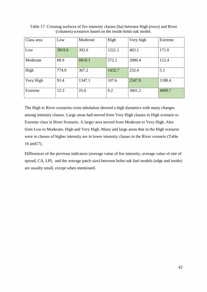
The High to River scenarios cross tabulation showed a high dynamics with many changes
among intensity classes. Large areas had moved from Very High classes in High scenario to
Extreme class in River Scenario. A larger area moved from Moderate to Very High. Also
from Low to Moderate, High and Very High. Many and large areas that in the High scenario
were in classes of higher intensity are in lower intensity classes in the River scenario (Table
16 and17).
Differences of the previous indicators (average value of fire intensity, average value of rate of
spread, CA, LPI, and the average patch size) between holm oak fuel models (edge and inside)
are usually small, except when mentioned.
43
5. Discussion
The main objective of this study was to understand and model the effects of holm oak
woodlands on fire behavior at the landscape level in Northeastern Portugal. Previous research
support the fact that holm oak woodlands have an effect on the spread and intensity of fire
(Azevedo et al., 2013), by controlling fuel loads at the ground level that decrease with
distance to woodland edge. Our results seem to further support that hypothesis since there is
an effect of decreasing average value of fire intensity and rate of spread over the gradient of
holm oak woodland occupancy in the landscape represented by the 4 scenarios tested.
Analysis of the spatial pattern of fire intensity classes with FRAGSTATS also seem to
provide evidence that increasing holm oak tends to reduce the size and dominance of higher
fire line intensity patches in the landscape.
The area of each fire intensity class among scenarios has changed (Figure 13). The classes
with high intensity have decreased in size, while those with low area have increased (High
and Very High) (Table 9; Figure 14).
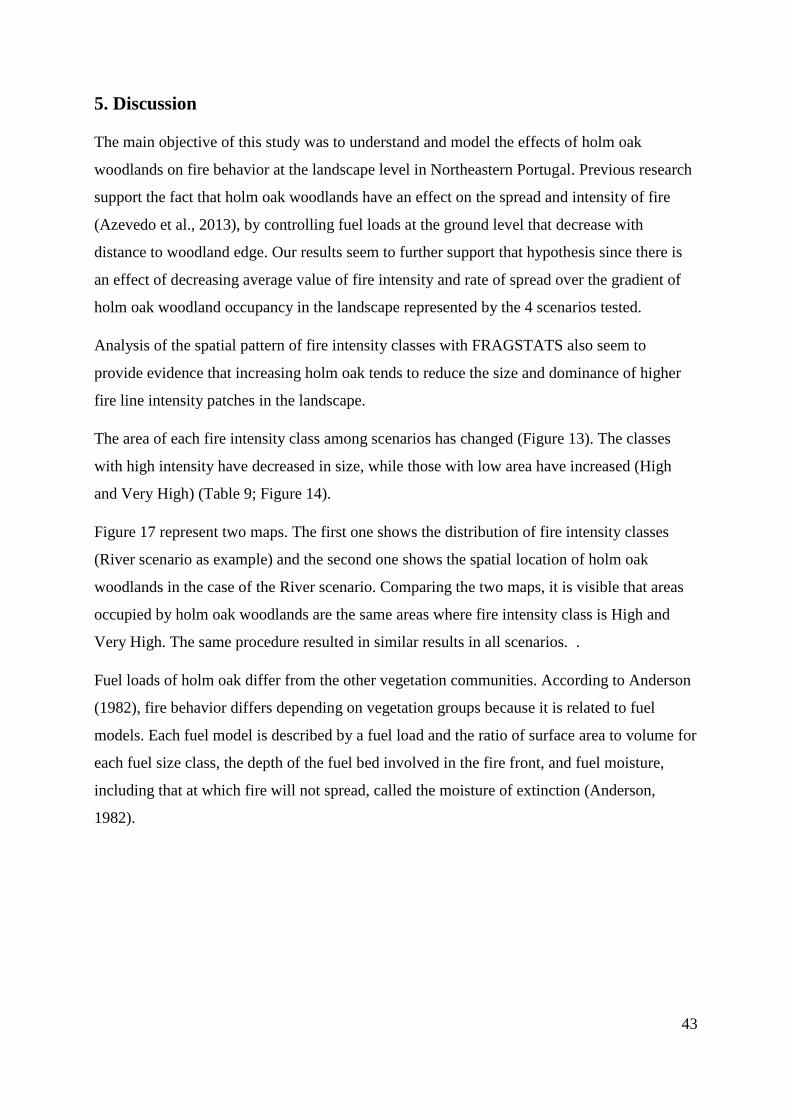
Figure 17 represent two maps. The first one shows the distribution of fire intensity classes
(River scenario as example) and the second one shows the spatial location of holm oak
woodlands in the case of the River scenario. Comparing the two maps, it is visible that areas
occupied by holm oak woodlands are the same areas where fire intensity class is High and
Very High. The same procedure resulted in similar results in all scenarios. .
Fuel loads of holm oak differ from the other vegetation communities. According to Anderson
(1982), fire behavior differs depending on vegetation groups because it is related to fuel
models. Each fuel model is described by a fuel load and the ratio of surface area to volume for
each fuel size class, the depth of the fuel bed involved in the fire front, and fuel moisture,
including that at which fire will not spread, called the moisture of extinction (Anderson,
1982).
44
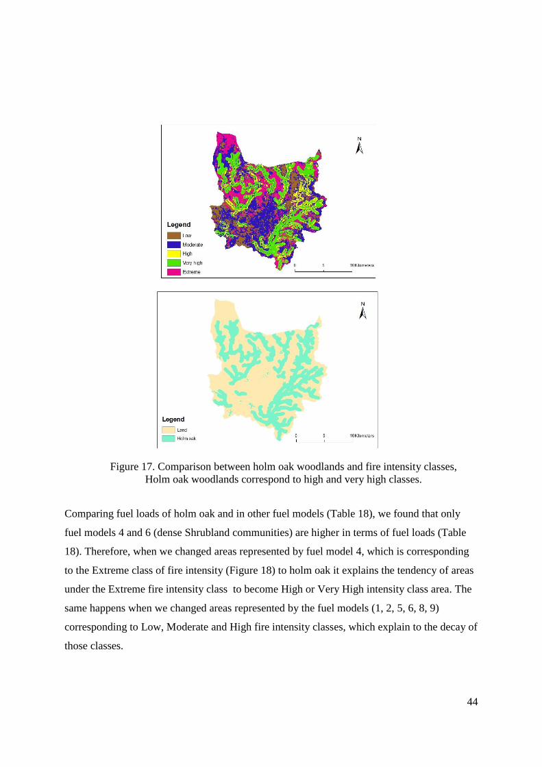
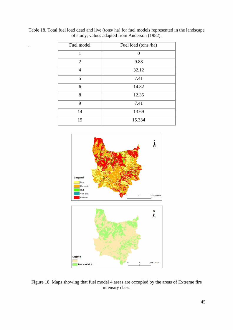
Comparing fuel loads of holm oak and in other fuel models (Table 18), we found that only
fuel models 4 and 6 (dense Shrubland communities) are higher in terms of fuel loads (Table
18). Therefore, when we changed areas represented by fuel model 4, which is corresponding
to the Extreme class of fire intensity (Figure 18) to holm oak it explains the tendency of areas
under the Extreme fire intensity class to become High or Very High intensity class area. The
same happens when we changed areas represented by the fuel models (1, 2, 5, 6, 8, 9)
corresponding to Low, Moderate and High fire intensity classes, which explain to the decay of
those classes.
Figure 17. Comparison between holm oak woodlands and fire intensity classes,
Holm oak woodlands correspond to high and very high classes.
45
Table 18. Total fuel load dead and live (tons/ ha) for fuel models represented in the landscape
of study; values adapted from Anderson (1982).
.
Figure 18. Maps showing that fuel model 4 areas are occupied by the areas of Extreme fire
intensity class.
Fuel model Fuel load (tons /ha)
1 0
2 9.88
4 32.12
5 7.41
6 14.82
8 12.35
9 7.41
14 13.69
15 15.334
46
Another explanation that can contribute in the analysis of our results is the fact that holm oak
fuel models are calibrated fuels for the northeastern Portugal region, contrarily to the others
fuels that are a standard ones and not specific for our study region.
Fire behavior in our study region, and the distribution of fire intensity classes are related
especially to the distribution of fuel models. This means that potential fire behavior for a fuel
type is expressed by fire hazard (MOF, 1997; Bachmann and Allgower, 2000; Hardy, 2005).
The fire hazard is applied to the fuel itself, for an instant or a period of time, without
including the weather or environs in which the fuel is distributed (Hardy, 2005).
47
6. Implications to management
Our results (Class area, LPI, and average patch size) provide information about potential
landscape structure and functioning and that can contribute also to improve our understanding
of the dynamics of landscape systems, which can be useful to suggest planning and
managements practices and activities at different scales.
The fact that all metrics (Class area, LPI, and average patch size), of all fire intensity classes
(Low, Moderate, High, Very High and Extreme) had decreased in scenarios with higher
percentage of holm oak (with exceptions). It means that higher fire intensity classes have less
relevance in the landscape and are also more fragmented which can be attributed to of holm
oak distribution. These results reveal that holm oak have a potential impact in the reduction of
fire hazard in the study area.
In the river scenario, metrics (Class area, LPI, and average patch size) had increased
compared to other scenarios, and this amount to the fact that holm oak areas are more
continuous comparing with the other scenarios; the holm oak woodlands are concentrated in
both sides of streams. According to Azevedo et al., (2011) the management priorities should
include: decreasing fire hazard at the patch level, increasing landscape heterogeneity and
decreasing connectivity of the most flammable land cover areas. In our case the results
obtained allows the identification of the most critical areas where management is more
exigent. Those areas correspond to Extreme fire intensity class (Figure 18).
The fact that holm oak woodlands affect fire behavior, eventually acting as barriers (Azevedo
et al. 2013) or just because they decrease the likelihood of large areas of very intensive
wildfires can have a significant in planning and management of landscapes for fire hazard
reduction, such as in preventive silviculture. From the results of our study, it seems reasonable
to admit that expanding holm oak woodlands in a scattered pattern to increase fragmentation
of higher fire intensity classes can contribute to an overall reduction of hazard. This
expansion, as was suggested by Azevedo et al. (2013), may be conducted artificially by
afforestation, or by promoting natural regeneration in abandoned areas that are those
corresponding to the areas where holm oak woodlands expanded in scenarios Moderate and
High.

48
Furthermore, in terms of landscape planning and management, additional information is
required to better address the use of holm oak woodlands in programs of conservation and
landscape fire hazard mitigation, including optimal patch size, shape, and orientation and
optimal proportion for holm oak woodlands and configuration in the landscape.
49
7. Conclusion
The main objective of our study was to understand and model the effect of holm oak
woodlands on fire behavior at the landscape level. The role of holm oak was determined in
terms of area and configuration of woodlands in the landscape according to the results
obtained from the scenarios built, based on the probable extension of these vegetation units.
The results demonstrate that holm oak woodlands have an effect on fire behavior by
decreasing the mean value of both fire intensity and rate of spread through scenarios (Low,
Moderate, High and River). The spatial pattern analysis of fire intensity classes (Low,
Moderate, High, Very High and Extreme) with FRAGSTATS also afford evidence that
increasing holm oak tends to reduce the size and dominance of higher fire line intensity
patches in the landscape. However, it is reasonable to admit that extending holm oak
woodlands in a sprinkled pattern to increase fragmentation of higher fire intensity classes can
contribute to an overall reduction of hazard.
To conclude, all the results that we had may contribute to improve the understanding of the
dynamics of landscape systems, which is useful to suggest planning and managements
practices and activities at different scales.

50
8. References
Agee, K. (1996). The Influence of Forest Structure on Fire Behavior. College of Forest
Resources, University of Washington, Seattle, Washington
Albini, F. (1976). Estimating wildfire behavior and effects. USDA Forest Service,
Intermountain Forest and Range Experiment Station. General Technical Report INT-
30–92 pp.
Alexander, J. D., Seavy, N. E., Ralph, C. J., & Hogoboom, B. (2006). Vegetation and
topographical correlates of fire severity from two fires in the Klamath-Siskiyou region
of Oregon and California. International Journal of Wildland Fire, 15(2), 237.
Alexander, M. E. (1982). Calculating and interpreting forest fire intensities. Canadian
Journal of Botany, 60(4), 349–357.
Alexander, M.E.; Lanoville, R.A. 1989. Predicting fire behavior in the black spruce-lichen
woodland fuel type of western and northern Canada. For. Can., North. For. Cent.,
Edmonton, Alberta, and Gov. Northwest Territ., Dep. Renewable Resour., Territ. For.
Fir Cent., Fort Smith, Northwest Territories.
Alexandrian, D., Esnault, F., Calabri, G. (1998). Forest fires in the Mediterranean area. (n.d.).
Retrieved June 25, 2016.
Allen, H. D. (2008). Fire: plant functional types and patch mosaic burning in fire-prone
ecosystems. Progress in Physical Geography, 32(4), 421–437.
Anderson, Hal E. 1982. Aids to determining fuel models for estimating fire behavior. USDA
For. Serv. Gen. Tech. Rep. INT-122, 22p.
Andrews, P. L. (2014). Current status and future needs of the BehavePlus Fire Modeling
System. International Journal of Wildland Fire, 23(1), 21.
51
Andrews PL (1986) ‘BEHAVE: Fire behavior prediction and fuel modeling system: BURN
subsystem, part 1.’ USDA Forest Service, General Technical Report INT-194.
(Ogden, UT)
Azevedo, J. C., Possacos, A., Aguiar, C. F., Amado, A., Miguel, L., Dias, R., Fernandes, P.
M. (2013). The role of holm oak edges in the control of disturbance and conservation
of plant diversity in fire-prone landscapes. Forest Ecology and Management, 297,
37–48.
Azevedo, J.C., Moreira, C., Castro, J.P., Loureiro, C., (2011). Agriculture abandonment,land-
use change and fire hazard in mountain landscapes in Northeastern Portugal. In:
Li, C., Lafortezza, R., Chen, J. (Eds.), Landscape Ecology in Forest Management and
Conservation: Challenges and Solutions for Global Change. HEP-Springer, Beijing,
pp. 329–351
Azevedo, J.C.; Possacos, A.; Dias, R.; Saraiva, A.; Loureiro, C.; Fernandes, P. (2009) -
Survival of holm oak woodlands in fire prone landscapes in Northeastern Portugal.
Latin American IALE Conference. Campos do Jordão, Brasil
Azevedo, J., Caçador, F., (2000). Bordaduras de bosques de Quercus rotundifolia Lam.
no Parque Natural de Montesinho. Quercetea 1, 126–137.
Bachmann, A., Allgower, B., (2000). The need for a consistent wildfire risk terminology. In:
Neuenschwander, L., Ryan, K., Golberg, G. (Eds.), Crossing the Millennium:
Integrating Spatial Technologies and Ecological Principles for a New Age in Fire
Management. The University of Idaho and the International Association of Wildland
Fire, Moscow, ID, pp. 67–77.
Bajocco, S., Pezzatti, G. B., Mazzoleni, S., & Ricotta, C. (2010). Wildfire seasonality and
land use: when do wildfires prefer to burn? Environmental Monitoring and
Assessment, 164(1–4), 445–452.
52
Bajocco, S., & Ricotta, C. (2008). Evidence of selective burning in Sardinia (Italy): which
land-cover classes do wildfires prefer? Landscape Ecology, 23(2), 241–248.
Barbero, M., Loisel, R., & Quézel, P. (1992). Biogeography, ecology and history of
Mediterranean Quercus ilex ecosystems. Vegetatio, 99–100(1), 19–34.
Booth, B., Mitchell, A., & Environmental Systems Research Institute (Eds.). (2001). Getting
started with ArcGIS: GIS ; [ArcGIS 8]. Redlands, Calif: Environmental Systems
Research Institute.
Bowman, D. M. J. S., Balch, J. K., Artaxo, P., Bond, W. J., Carlson, J. M., Cochrane, M. A.,
Pyne, S. J. (2009). Fire in the Earth System. Science, 324(5926), 481–484.
Broncano, M. J., Retana, J., & Rodrigo, A. (2005). Predicting the Recovery of Pinus
halepensis and Quercus ilex Forests after a Large Wildfire in Northeastern Spain.
Plant Ecology, 180(1), 47–56.
Catry, F. X., Rego, F., Moreira, F., Fernandes, P. M., & Pausas, J. G. (2010). Post-fire tree
mortality in mixed forests of central Portugal. Forest Ecology and Management,
260(7), 1184–1192.
Davies, K. W., Boyd, C. S., Bates, J. D., & Hulet, A. (2016). Winter grazing can reduce
wildfire size, intensity and behaviour in a shrub-grassland. International Journal of Wildland
Fire, 25(2), 191.
DeWilde, L., & Chapin, F. S. (2006). Human Impacts on the Fire Regime of Interior Alaska:
Interactions among Fuels, Ignition Sources, and Fire Suppression. Ecosystems, 9(8),
1342–1353.
Dias R, Azevedo J. (2008). Distribution and spatial configuration of holm oak woodlands in
the Montesinho/Nogueira site, Portugal.
53
Duncan, B. W., Schmalzer, P. A., Breininger, D. R., & Stolen, E. D. (2015). Comparing fuels
reduction and patch mosaic fire regimes for reducing fire spread potential: A spatial
modeling approach. Ecological Modelling, 314, 90–99.
Ellsworth, L. M., Litton, C. M., Dale, A. P., & Miura, T. (2014). Invasive grasses change
landscape structure and fire behaviour in Hawaii. Applied Vegetation Science, 17(4),
680–689.
Catry, F. X., Moreira, F., Rego, F., Branco, M., & Sousa, E. (2014). Fire-induced bark beetle
attacks in Mediterranean cork oak forests: which factors drive host selection?
Finney, M. A. (2006). An overview of FlamMap fire modeling capabilities.(link is
external) In: Fuels management—how to measure success: conference proceedings.
2006 March 28-30; Portland, Oregon. Proceedings RMRS-P-41. Fort Collins, CO:
U.S. Department of Agriculture, Forest Service, Rocky Mountain Research Station:
213-220.
Forghani, A., Kazemi, S., & Ge, L. (2014). Wildland Fire Behaviour Simulations Employing
an Integrated Weather-Topographical-Fuel Datasets and Satellite Remote
Sensing. International Journal of Geoinformatics, 10(4), 35-44.
Gonçalves, J.A., Morgado, A. (2008). Use of the SRTM DEM as a geo-referencing tool by
elevation matching. International Archives Photogrammetry, Remote Sensing and
Spatial Information Sciences..
Gonçalves, J.A., Fernandes, J.C. (2005). Assessment of SRTM-3 DEM in Portugal with
topographic map data. EARSeL 3D Remote Sensing Workshop, Porto, Portugal, 6-11
June, 2005.
Hardy, C. C. (2005). Wildland fire hazard and risk: Problems, definitions, and context. Forest
Ecology and Management, 211(1–2), 73–82.
54
Hollingsworth, L. T., Kurth, L. L., Parresol, B. R., Ottmar, R. D., & Prichard, S. J. (2012). A
comparison of geospatially modeled fire behavior and fire management utility of three
data sources in the southeastern United States. Forest Ecology and Management, 273,
43–49.
Jain, T., Pilliod, D., Graham, R. (2004). Tongue-tied. Wildfire, 4, 22–36.
Keane, Robert E.; Cary, Geoffrey J.; Flannigan, Mike D. (2011). Challenges and needs in fire
management: A landscape simulation modeling perspective [chapter 4]. In: Li, C.;
Lafortezza, R.; Chen, J., eds. Landscape ecology in forest management and
conservation: Challenges and solutions for global change. Beijing, China: Springer,
Higher Education Press. p. 75-98.
Keeley, J. E. (2009). Fire intensity, fire severity and burn severity: a brief review and
suggested usage. International Journal of Wildland Fire, 18(1), 116.
Khabarov, N., Krasovskii, A., Obersteiner, M., Swart, R., Dosio, A., San-Miguel-Ayanz, J.,
Migliavacca, M. (2016). Forest fires and adaptation options in Europe. Regional
Environmental Change, 16(1), 21–30.
Lentile, L. B., Holden, Z. A., Smith, A. M. S., Falkowski, M. J., Hudak, A. T., Morgan, P., …
Benson, N. C. (2006). Remote sensing techniques to assess active fire characteristics
and post-fire effects. International Journal of Wildland Fire, 15(3), 319.
Marlier, M. E., DeFries, R. S., Voulgarakis, A., Kinney, P. L., Randerson, J. T., Shindell, D.
T., … Faluvegi, G. (2012). El Niño and health risks from landscape fire emissions in
southeast Asia. Nature Climate Change, 3(2), 131–136.
McCaw, W. L., & Burrows, N. D. (1989). Fire management. In B. Dell, J. J. Havel, & N.
Malajczuk (Eds.), The Jarrah Forest (pp. 317–334).
55
McGarigal, K., and B.J. Marks. (1995). FRAGSTATS: spatial pattern analysis program for
quantifying landscape structure. Gen. Tech. Report PNW-GTR-351, USDA Forest
Service, Pacific Northwest Research Station, Portland, OR.
Ministry of Forests (MOF), (1997). Glossary of Forest Terms. Ministry of Forests, Province
of British Columbia, Canada.
Nunes, M. C. S., Vasconcelos, M. J., Pereira, J. M. C., Dasgupta, N., Alldredge, R. J., &
Rego, F. C. (2005). Land Cover Type and Fire in Portugal: Do Fires Burn Land Cover
Selectively? Landscape Ecology, 20(6), 661–673.
Parsons, A. (2003). Burned Area Emergency Rehabilitation (BAER) soil burn severity
definitions and mapping guidelines. Draft. USDA Forest Service, Rocky Mountain
Research Station. (Missoula, MT)
Pausas, J. G., & Vallejo, V. R. (1999). The role of fire in European Mediterranean
ecosystems. In E. Chuvieco (Ed.), Remote Sensing of Large Wildfires (pp. 3–16).
Berlin, Heidelberg: Springer Berlin Heidelberg.
Perera, A. H., Dalziel, B. D., Buse, L. J., & Routledge, R. G. (2009). Spatial variability of
stand-scale residuals in Ontario’s boreal forest fires. Canadian Journal of Forest
Research, 39(5), 945–961.
Pimont, F., Parsons, R., Rigolot, E., de Coligny, F., Dupuy, J.-L., Dreyfus, P., & Linn, R. R.
(2016). Modeling fuels and fire effects in 3D: Model description and applications.
Environmental Modelling & Software, 80, 225–244.
Plucinski, M. P. (2014). The timing of vegetation fire occurrence in a human landscape. Fire
Safety Journal, 67, 42–52.
Rothermel, Richard C. (1983). How to predict the spread and intensity of forest and range
fires. Gen. Tech. Rep. INT-143. Ogden, UT: U.S. Department of Agriculture, Forest
Service, Intermountain Forest and Range Experiment Station. 1 61 p.
56
Rothermel, R. C. (1982). Modelling the Development of Fire in a Forest Environment. In T.
van Nao (Ed.), Forest Fire Prevention and Control (Vol. 7, pp. 77–84). Dordrecht:
Springer Netherlands.
Rothermel, Richard C. (1972). A mathematical model for fire spread predictions in wildland
fuels. USDA For. Serv. Res. Pap. INT-115, 40 p. lntermt. For. and Range Exp. Stn.,
Ogden, Utah.
Scott, Joe H. (2012). Introduction to Wildfire Behavior Modeling. National Interagency Fuels,
Fire, & Vegetation Technology Transfer.
Scott, Joe H.; Burgan, Robert E. 2005. Standard fire behavior fuel models: a comprehensive
set for use with Rothermel’s surface fire spread model. Gen. Tech. Rep. RMRS-GTR-
153. Fort Collins, CO: U.S. Department of Agriculture, Forest Service, Rocky
Mountain Research Station. 72 p
Silva, J. S., & Catry, F. (2006). Forest fires in cork oak (Quercus suber L.) stands in Portugal.
International Journal of Environmental Studies, 63(3), 235–257.
Simard, S. (1991). Fire Severity, Changing Scales, and How Things Hang Together.
International Journal of Wildland Fire, 1(1), 23.
STARFIRE project, Fire behavior and FlamMap, 2011.
Terradas, J. (1999). Holm Oak and Holm Oak Forests: An Introduction. In F. Rodà, J. Retana,
C. A. Gracia, & J. Bellot (Eds.), Ecology of Mediterranean Evergreen Oak Forests
(Vol. 137, pp. 3–14).
Velez, R. (1982). Forest Fires in the Mediterranean Region. In T. van Nao (Ed.), Forest Fire
Prevention and Control (Vol. 7, pp. 37–51).
Viedma, O. (2008). The influence of topography and fire in controlling landscape
composition and structure in Sierra de Gredos (Central Spain). Landscape Ecology,
23(6), 657–672.

57
Viedma, O., Angeler, D. G., & Moreno, J. M. (2009). Landscape structural features control
fire size in a Mediterranean forested area of central Spain. International Journal of
Wildland Fire, 18(5), 575.