Embed Size (px)
Citation preview

Simplicial Cohomology of Totally
Ordered Semigroup Algebras
David Peter Elliott
Thesis submitted for the degree of
Doctor of Philosophy
School of Mathematics and Statistics
Newcastle University
Newcastle upon Tyne
United Kingdom
June 2012

Acknowledgements
One of the most poignant pieces of advice given to me when considering my PhD
was that choosing the right supervisor is just as important, if not more so, than
the topic you choose to research. To that end I believe I was in the strongest
possible position throughout my studies and started with the battle half won.
Therefore, first and foremost, my heartfelt thanks must go to my supervisor,
Michael White, whose mathematical insight, humour and patience cannot be
(co)bounded. I am also grateful for his constant encouragement, guidance and
supreme flexibility, especially with his time and my work turnaround.
Being able to do my PhD would not have been possible without the financial
support provided to me by EPSRC, to whom I am extremely grateful. I would
also like to thank the School of Mathematics and Statistics for their constant and
uplifting support over the years.
My examiners, Joel Feinstein and Zina Lykova, also deserve a special thanks for
their time and attention to detail, putting me through the wringer and really
making me feel like I earned my pass.
Without my fellow PhD students I am entirely certain I would have retained far
less of my sanity than I managed to; therefore I would like to thank them for
their encouragement and comradeship over the years, which was and is so very
valuable to me. In particular I am grateful to Kevin, my constant companion
on this journey and others, Daniel, my gracious housemate, and the five-a-siders,
helping me to blow off steam and putting up with me when my venting became
intense.
In producing this thesis some technical help has been necessary for me to avoid
writing everything in crayon. First, my thanks must go to Paul Taylor, whose
diagrams.sty package I have used extensively throughout my work. Second, and
very importantly, my eternal thanks to resident TEX-pert Anthony Youd, without
whom this work would have been far shorter (and uglier), not least for the use of
his superlative thesis template.

Being able to step outside of the academic bubble on a regular basis has gone
a long way to helping me recharge and stay sharp. Thus to the Air Training
Corps and its wonderful personnel, especially my friends and colleagues, I am,
and always will be, extremely grateful.
My sincere thanks must go to my parents and family for their constant support
and encouragement, not just for my PhD but for everything, helping me through
the lows and accompanying me through the highs, despite never actually knowing
just what it is that I do no matter how many times I try to explain.
And finally my fondest and heartfelt thanks go to Helene, my confidante and my
rock, for always being there and offering me unwavering support, for helping me
see the way forward and for so much more I cannot express here in mere words.
Thank you for making this even more meaningful.

Abstract
It is known that some discrete semigroup algebras have trivial continuous simpli-
cial cohomology, at least in high dimensions. The aim of this work is to investigate
the situation for the locally compact case, which even for the important example
of the positive real numbers is not clear.
The initial focus of this thesis is on the continuous simplicial cohomology groups
for the algebra L1(R+, ∨). We then adapt our methods and progress to investi-
gating the more general case of L1(X,≤, µc) where (X,≤) is a totally ordered
semigroup with the binary operation max and which is locally compact in its
order topology and µc is a continuous, σ-finite, positive, regular Borel measure
on X.
The first continuous simplicial cohomology of L1(R+, ∨) was already known, but
we offer a new method of deriving this result and then use this method to prove
the triviality of higher dimensional continuous simplicial cohomology groups for
this algebra. We then modify our method to derive analogous results for the
algebra L1(X,≤, µc) by analysing the algebra L1(R+, µc).
Contents
1 Introduction 1
1.1 Motivation . . . . . . . . . . . . . . . . . . . . . . . . . . . . . . . 1
1.2 Recent work . . . . . . . . . . . . . . . . . . . . . . . . . . . . . . 2
1.3 Section by section overview . . . . . . . . . . . . . . . . . . . . . 5
2 Preliminaries 7
2.1 Banach semigroup convolution algebras . . . . . . . . . . . . . . . 7
2.2 Homological algebra and simplicial cohomology . . . . . . . . . . 22
2.2.1 Cochain complexes . . . . . . . . . . . . . . . . . . . . . . 23
2.2.2 Hochschild, simplicial and cyclic (co)homology . . . . . . . 25
2.2.3 Connes-Tzygan long exact sequence . . . . . . . . . . . . . 29
3 The first simplicial cohomology group of `1(Z+, ∨) and L1(R+, ∨) 30
3.1 Derivations . . . . . . . . . . . . . . . . . . . . . . . . . . . . . . 31
3.2 Weak amenability in the discrete case . . . . . . . . . . . . . . . . 32
3.3 Weak amenability in the locally compact case . . . . . . . . . . . 36
4 The second simplicial cohomology group of `1(Z+, ∨) and L1(R+, ∨) 54
4.1 The discrete case . . . . . . . . . . . . . . . . . . . . . . . . . . . 55
4.2 The locally compact case . . . . . . . . . . . . . . . . . . . . . . . 65
4.3 An example of cobounding a particular cyclic 2-cocycle . . . . . . 83
i
Contents
4.4 An example of an algebra with nontrivial second simplicial coho-
mology . . . . . . . . . . . . . . . . . . . . . . . . . . . . . . . . . 85
5 The general simplicial cohomology group of L1(R+, ∨) 90
5.1 Re-evaluating the second simplicial cohomology group . . . . . . . 92
5.1.1 Cobounding a 2-cocycle on a particular ordering of arguments 92
5.1.2 The remaining cases . . . . . . . . . . . . . . . . . . . . . 117
5.2 Investigating the nth simplicial cohomology group of L1(R+, ∨) . . 124
5.2.1 Contracting homotopy . . . . . . . . . . . . . . . . . . . . 125
5.2.2 Constructing our contracting homotopy in degree n . . . . 126
5.2.3 A locally compact case . . . . . . . . . . . . . . . . . . . . 134
5.2.4 The locally compact case in degree n . . . . . . . . . . . . 138
6 A more general class of locally compact semigroup algebras 140
6.1 Some definitions . . . . . . . . . . . . . . . . . . . . . . . . . . . . 141
6.2 Borel measures . . . . . . . . . . . . . . . . . . . . . . . . . . . . 142
6.3 The diagonal in R+ . . . . . . . . . . . . . . . . . . . . . . . . . . 143
6.4 Adjusting the spreading out function . . . . . . . . . . . . . . . . 148
6.4.1 The inverse to the spreading out function . . . . . . . . . . 150
6.4.2 The approximate module property . . . . . . . . . . . . . 151
6.5 The simplicial cohomology groups of L1(R+,≤, µc) . . . . . . . . . 152
6.6 Extending to a general totally ordered, locally compact semigroup 154
7 Conclusions and further work 166
ii

Chapter 1
Introduction
Cohomology arose as a natural part of algebraic topology, growing over the years
to occupy a fundamental place within several areas of pure mathematics.
A large and increasing variety of cohomology theories exist, each offering insights
into other areas of mathematics and providing tools with which we are able to
explore even further.
The aim of this thesis is to consider an analytical version of Hochschild coho-
mology, particularly simplicial cohomology, for certain Banach algebras. In this
chapter we will give some motivation and historical context for considering such
problems.
1.1 Motivation
The dual notion to homology and considered by functional analysts the more
natural course of study due to the appearance of dual spaces and functionals,
cohomology was first glimpsed in Henri Poincare’s duality theorem in the 1890s
(for more see §3.3 in [19]). The idea was made more formal over the next few
decades and diverged into a wide class of cohomology theories such as de Rham
cohomology, Cech cohomology and of course Hochschild cohomology.
All of these theories are algebraically based and mostly centre around groups or
algebraic objects. Several mathematicians attempted to extend these methods to
a Banach algebra setting in the 1960s and early 1970s.
1

Chapter 1. Introduction
One of the first attempts was made by Herbert Kamowitz who investigated con-
tinuous cohomology groups for commutative C∗-algebras with, as we would say,
coefficients in commutative or finite Banach modules. Alain Guichardet followed
this up by defining homology and cohomology groups and investigating their re-
lationships before considering certain cases involving the group algebra L1(G) for
some group G.
Alexander Helemskiı, who has since made even more progress in this field (see
his book, [20]), introduced the concept of normed modules over Banach algebras
at about the same time J.L.Taylor considered topological algebras.
The biggest step came in 1972 when Barry Johnson published his memoir Coho-
mology in Banach Algebras [23], placing the definitions of Hochschild cohomology
in a Banach algebra setting on a firm footing, as well as adapting the notion of
amenability. After this W.G.Bade, P.C.Curtis and H.G.Dales [1] were able to
define the concept of weak amenability for commutative Banach algebras, par-
ticularly Beurling and Lipschitz algebras, which was naturally extended to all
Banach algebras by Johnson himself, and N.Grønbæk looked at bounded deriva-
tions from L1(R+, w) into its dual for a weight function w.
I would like to thank Dr Zinaida Lykova and Dr Volker Runde for providing me
with extra insight into the history behind simplicial cohomology through their
illuminating seminar talks.
1.2 Recent work
This thesis builds upon some more recent work in this area. The research of
T.D.Blackmore, the quartet Y.Choi, F.Gourdeau, Z.A.Lykova and M.C.White,
who have worked independently and in various collaborations, Baker, Pym, Va-
sudeva and Helemskiı in particular has considered several problems similar to
those in my work.
A lot of work has been done on simplicial cohomology for discrete algebras, that
is those algebras with an underlying discrete measure. In [17] Gourdeau and
White showed that the third simplicial cohomology group for the algebra `1(Z+),
where the binary operation on the underlying semigroup is addition, is trivial.
2

Chapter 1. Introduction
Gourdeau and White with B.E.Johnson in [13] showed that for the algebra `1(N),
again with addition serving as the binary operation on the underlying semigroup,
the cyclic cohomology groups are trivial in odd degree and one dimensional in
even degree above two which implies, via the Connes-Tzygan long exact sequence,
that the simplicial cohomology groups vanish in degree two and higher.
Increased dimensionality of the underlying semigroup is the subject for Gour-
deau, Lykova and White in [15] where, amongst other things, they look at the
simplicial cohomology groups for `1(Zk+). In this paper they show that the sim-
plicial cohomology groups are Banach spaces, and the nth groups are trivial when
n ≥ k and nonzero otherwise for n ∈ N.
Much of the ground work in extending the ideas of Johnson in [23] was done by
Alexander Helemskiı. In particular his book [20] considers the homology of Ba-
nach and topological algebras and gives a lot of the required definitions, including
general concepts, using tensor products and resolutions among others. His paper
[21] is also of great importance as it considers the links between simplicial and
cyclic cohomology through the Connes-Tzygan long exact sequence, which we
make use of extensively throughout this thesis.
Yemon Choi, both in his PhD thesis and afterwards, has done a lot of work
in this area. In particular his paper [8] showed that the `1-convolution algebra
of a semilattice with symmetric coefficients has trivial simplicial cohomology in
all degrees greater than or equal to one. In [9] he extends the work done by
Gourdeau, Lykova and White in [15] by considering more general symmetric
coefficients among other things. This work is extended in collaboration with
Gourdeau and White in [10] where they investigate simplicial triviality for the
`1-convolution algebra of a band semigroup.
Gourdeau and White also looked at simplicial cohomology for the bicyclic semi-
group algebra via an interesting admissible resolution approach and the Connes-
Tzygan long exact sequence in [18]. They obtained once again that the cyclic
cohomology groups vanish in odd degree and are one-dimensional in even de-
gree greater than two while the simplicial cohomology groups all vanish in degree
greater than or equal to two.
T.D.Blackmore in his Ph.D thesis and subsequent papers concerned himself with
weak amenability, that is the first simplicial cohomology groups, for certain Ba-
3

Chapter 1. Introduction
nach algebras. In [4] he, amongst other things, investigated the weak amenability
of `1-convolution algebras of algebraic discrete semigroups with a weight function.
Although a lot of analysis has been conducted in the discrete case the level of
consideration of what happens when the underlying measure on a semigroup is
continuous, or a combination of continuous and discrete measures, is not nearly
so expansive.
In their paper [2] Baker, Pym and Vasudeva considered compact totally ordered
measure spaces and investigated their Lp algebras. They formalised important
definitions and concepts, such as how to impose multiplication on such algebras.
In addition to this they also analysed the links to Gelfand transforms and iso-
morphisms between Lp algebras of spaces with regular continuous measures on
them. A very important theorem they put forward states that the algebra Lp(µ)
for a regular continuous measure µ is commutative and semisimple for 1 ≤ p ≤ ∞and that for p = 1 this algebra has a bounded approximate identity. They also
considered multipliers but that is of little concern to us in this thesis.
Gourdeau, Lykova and White have produced numerous results in investigating the
simplicial cohomology of L1(Rk+,+). In [14] they showed that the nth simplicial
cohomology groups for L1(Rk+,+) are trivial when n ≥ k and nontrivial otherwise
for n ∈ N.
The other main work in this area, and the paper on which this thesis starts
and builds, is Blackmore’s paper on derivations from totally ordered semigroup
algebras into their duals [3]. In this work Blackmore considered totally ordered
semigroups X which are locally compact in their order topology and have an
underlying σ-finite, regular, positive Borel measure µ. He stated that the measure
can be uniquely decomposed into its discrete and continuous parts, µd and µc
respectively, and then went on to investigate each part independently. He arrived
at the conclusion that the first simplicial cohomology group for the L1 algebra
for the discrete part, L1(X,µd), is trivial while the continuous part, L1(X,µc), is
isomorphic to its dual. He also went on to investigate the bounded derivations
from Lp([0, 1],m) into its dual for 1 ≤ p <∞ and m Lebesgue measure, but that
is not followed up in the present work.
4
Chapter 1. Introduction
1.3 Section by section overview
The work in this thesis is concerned with analysing the higher simplicial coho-
mology groups for the continuous part of the measure in the case Blackmore
considered when investigating bounded derivations. It furthers his work in that
we consider the higher dimensional simplicial cohomology groups of certain semi-
group algebras and consider cyclic cohomology groups as well. It is also in some
respects a complement to the work of Gourdeau, Lykova and White in [14] in
that we consider as part of this work the simplicial cohomology groups of L1(R+).
However where they considered the binary operation on the underlying semigroup
to be addition we use the max operation instead. Additionally, the methods used
here to approach this problem are different from those used by Gourdeau, Lykova
and White and allow the analysis of a more general class of Banach semigroup
algebras.
The initial groundwork is laid out in Chapter 2, where the main definitions and
core results we will need are given. We define Banach semigroup convolution
algebras in the discrete and continuous case; for clarity we refer to these last as
locally compact. We also give the necessary definitions of homological algebra and
simplicial cohomology before looking at the Connes-Tzygan long exact sequence,
a fundamental tool we will make repeated use of throughout this work.
Chapter 3 proves the same result given by Choi, Gourdeau and White in [10]
and Johnson in [24] concerning the triviality of the first simplicial cohomology
group of `1(Z+, ∨), but we use a different methodology for doing this. We then
use this method to obtain the same result given by Blackmore in [3] regarding
the isomorphism between the first simplicial cohomology group of L1(R+, ∨) and
its dual space again in a different way.
The purpose of Chapter 3 is to create a method which we could use to analyse
the higher dimensional cohomology groups; by obtaining the same results as
before we have validated these methods, and in Chapter 4 we adapt and apply
them to the second simplicial cohomology group of L1(R+, ∨) by once again first
gaining insight via the case when the algebra under consideration is `1(Z+, ∨).
We do this by first considering the cyclic cohomology groups and attempting to
cobound a given 2-cocycle, investigate its required properties, show that the cyclic
cohomology group is trivial and then show that simplicial cohomology groups are
5
Chapter 1. Introduction
also trivial by using the Connes-Tzygan long exact sequence.
The closing stages of Chapter 4 give an example of cobounding a specific 2-cocycle
and then an example of a semigroup algebra with non-vanishing second simplicial
cohomology.
We once again modify our methods slightly in Chapter 5 where we show that
the nth simplicial cohomology group for L1(R+, ∨) vanishes. The substance of
the chapter is concerned with generalising our method to n dimensions and then
applying it to get the main result.
Chapter 6 considers the general case, that of the algebra L1(X,≤, µc) where
(X,µc) is a totally ordered semigroup which is locally compact in its order topol-
ogy and µc is a continuous, σ-finite, positive, regular Borel measure on X. Some
necessary definitions are given before we once more adapt and extend our method
to deal with this general case before giving the last main result, which is that the
simplicial cohomology groups in this case are isomorphic to the dual space of the
semigroup algebra in degree one and trivial in all higher degrees.
This thesis is then rounded off in Chapter 7 where the main points are summarised
and some other questions naturally arising from this work are proposed for further
research.
6

Chapter 2
Preliminaries
Many of the central concepts and common results that form much of the back-
ground for the work contained in this thesis can be found in many publications
including [20] and [5]. The papers [2] and [3] also contain many of these defini-
tions in a very similar form. We present some of the notation and terminology
that is key to obtaining our results here for further clarity.
Throughout this section all vector spaces are defined using the underlying ground
field of C as this is the convention we use. However they are also applicable for
any other field F.
The notions of chain maps and chain homotopies are used in later sections and
more background on these can be found in [30]. Although not explicitly used an
underlying topic here is that of category theory; [22] gives a nice introduction to
categories and functors.
2.1 Banach semigroup convolution algebras
In this section we introduce the concepts of semigroup convolution algebras, giv-
ing some basic but useful definitions. We then focus particularly on the algebras
the work in this thesis is centred around.
Definition. Let S be a set with an associative binary operation · : S × S → S
7

Chapter 2. Preliminaries
mapping (s, t) to s · t, i.e. such that
(s · t) · r = s · (t · r) ∀s, t, r ∈ S. (2.1)
Then S is called a semigroup and its associated binary operation is referred to
as multiplication. For convenience we often omit the symbol · and simply write
st for s · t.
In the case where it is necessary to identify the binary operation · associated with
a semigroup S we will write this as (S, ·).
Notice that the condition for being a semigroup is one of the three requirements
of a group; therefore every group is also a semigroup. If a semigroup S has an
identity 1 ∈ S such that 1 · s = s · 1 = s for all s ∈ S then we have satisfied a
second condition for being a group and we call S a monoid.
Proposition 2.1. Let S be a monoid with identities 1 and e. Then 1 = e.
The proof is trivial, mimicking the proof for the analogous result for groups, and
can be found in many books on algebra, for example [12]. Thus it is unambiguous
to talk about the identity element of S.
Discrete semigroup algebras
Definition. Let (S, ·) be a countable semigroup. Then we define
`1(S, ·) =
{f : S → C : f =
∑s∈S
asδs with∑s∈S
|f(s)| =∑s∈S
|as| <∞
}, (2.2)
where as ∈ C and for t ∈ S
δs(t) =
1, s = t,
0, s 6= t.(2.3)
Once again when the binary operation is unambiguous we will simply suppress the
symbol and write `1(S). In fact a natural binary operation which we impose on
this semigroup when constructed to be locally compact within its order topology,
8

Chapter 2. Preliminaries
which we consider in a later case, is maximum multiplication, and we use this
throughout the thesis.
We define addition and scalar multiplication on `1(S, ∨) to be pointwise and give
it a multiplication ∗ defined by convolution,
(f ∗ g)(s) =∑tu=s
f(t)g(u), s, t, u ∈ S. (2.4)
We define this sum to be zero if tu = s has no solutions. The usual norm for this
space is given by
‖f‖ =∑s∈S
|f(s)| (2.5)
for f ∈ `1(S, ∨). It is a well-known result that this is a Banach algebra and it is
called the discrete semigroup algebra of S.
We now look at a specific example of a discrete semigroup algebra, one which we
shall consider carefully in further chapters.
The discrete semigroup algebra of (Z+, ∨)
Consider the semigroup which is given by the set of nonnegative integers and the
binary operation of ∨ : Z+ × Z+ → Z+ given by
x∨y = max{x, y}, x, y ∈ Z+. (2.6)
We denote this semigroup as (Z+, ∨). This is in fact a monoid, with identity
element 0.
Since the underlying semigroup here is discrete the corresponding discrete semi-
group algebra is in fact a space of sequences. Thus given a function f ∈ `1(Z+, ∨)
we can write this as a series
f =∞∑n=0
anδn, (2.7)
9

Chapter 2. Preliminaries
where an ∈ C and for m ∈ Z+
δn(m) =
1, n = m,
0, n 6= m.(2.8)
The usual norm on this algebra is by definition given by ‖f‖ =∑∞
n=0 |an|, and
the formula for multiplying two elements f, g ∈ `1(Z+, ∨) given by f =∑∞
t=0 atδt
and g =∑∞
u=0 buδu, for at, bu ∈ C, t, u ∈ Z+, can then be simplified for N ∈ Z+
as
(f ∗ g)(N) =∑
n∨m=N
f(n)g(m)
=∑
n∨m=N
{(∞∑t=0
atδt(n)
)(∞∑u=0
buδu(m)
)}=
∑n∨m=N
anbm
= aN
N∑m=0
bm + bN
N−1∑n=0
an.
(2.9)
This is also consistent with simply multiplying f and g as defined above together
in the usual way. The summation range of the second term does not include the
endpoint N because that term has already appeared in the first sum. We could
equally well have written the summation limits the other way around instead,
but have chosen not to and this does not affect the overall meaning.
Notice that for fixed t, u we have
(δt ∗ δu)(N) =∑
n∨m=N
δt(n)δu(m). (2.10)
If t∨u 6= N then every term in this sum is zero. On the other hand, if t∨u = N
then exactly one term in this sum is nonzero, namely δt(t)δu(u), which has value
1. Therefore we have that
(δt ∗ δu)(N) =
1, t∨u = N,
0, t∨u 6= N,(2.11)
10

Chapter 2. Preliminaries
which is the same as δt∨u(N).
Definition. Let A and B be algebras over C. A linear mapping φ from A into
B such that
φ(xy) = φ(x)φ(y), x, y ∈ A, (2.12)
is called a homomorphism. If φ is injective we call it a monomorphism, surjective
an epimorphism and bijective an isomorphism.
Definition. Let A be an algebra over C. A character on A is a nonzero linear
homomorphism mapping A into the field C (i.e. a multiplicative functional).
Where A is a Banach algebra it automatically follows that all characters are
bounded and hence continuous; see §16 in [5]. The space of all characters on A
is denoted by M(A).
Proposition 2.2. Let f, g ∈ `1(Z+, ∨) be given by f =∞∑n=0
anδn and g =∞∑m=0
bmδm
respectively and define χM : `1(Z+, ∨)→ C for M ∈ N ∪ {∞} by
χM(f) =∑n<M
an. (2.13)
Then χM is a character. Furthermore, all characters χ ∈ M(`1(Z+, ∨)) are of
this form.
It should be noted that the calculations of such characters are relatively simple
to perform. The result is Banach algebra folklore.
Proof. First, we show that χM is linear. Let λ ∈ C. Then we have
χM(f + λg) = χM
(∞∑n=0
anδn +∞∑m=0
λbmδm
)
= χM
(∞∑k=0
(ak + λbk)δk
)=∑k<M
(ak + λbk)
=∑k<M
ak + λ∑k<M
bk
= χM(f) + λχM(g).
(2.14)
11

Chapter 2. Preliminaries
Note that it is enough to prove the relation holds for the generators δn, δm. For
if
χM(δn)χM(δm) = χM(δn∨m), (2.15)
then
χM(anδn)χM(bmδm) = χM(anbmδn∨m). (2.16)
By linearity and continuity this extends to give
⇒ χM
(∞∑n=0
anδn
)χM
(∞∑m=0
bmδm
)= χM
(∞∑n=0
∞∑m=0
anbmδn∨m
), (2.17)
which is simply χM(f)χM(g) = χM(f ∗ g) since
f ∗ g =
(∞∑n=0
anδn
)(∞∑m=0
bmδm
)
=∞∑n=0
∞∑m=0
anbmδnδm
=∞∑n=0
∞∑m=0
anbmδn∨m.
(2.18)
So it remains to prove that χM(δn)χM(δm) = χM(δn∨m), i.e.0, if n ≥M,
1, if n < M,×
0, if m ≥M,
1, if m < M,=
0, if n∨m ≥M,
1, if n∨m < M.(2.19)
It is clear that the LHS 6= 0 when both n,m < M and occurs if, and only if,
n∨m < M , which is the condition for the RHS 6= 0.
Finally we prove that all characters χ ∈ M(`1(Z+, ∨)) are of the form χM . Note
that χ(δn ∗ δn) = χ(δn) and so it follows that χ(δn) is equal to either 0 or 1.
It must be that if χ(δN) = 0 for some N ∈ Z+ that χ(δn) = 0 for all n ≥ N . To
show this let N ∈ N be such that χ(δN) = 0 and let m ∈ N be such that m ≥ N .
12
Chapter 2. Preliminaries
It follows that
χ(δm) = χ(δm ∗ δN)
= χ(δm) · χ(δN)
= χ(δm) · 0,
(2.20)
and so χ(δm) = 0 for all m ≥ N .
If χ(δm) 6= 0 for all m ∈ Z+, i.e. there is no instance of χ(δm) = 0, then
χ(f) = χ
(∞∑n=0
anδn
)
=∞∑n=0
anχ(δn)
=∞∑n=0
an · 1
= χ∞(f).
(2.21)
Now suppose that N is the first instance when χ(δn) = 0 for n ∈ Z+ and therefore
χ(f) = χ
(∞∑n=0
anδn
)
=∞∑n=0
anχ(δn)
=N−1∑n=0
an · 1
= χN(f).
(2.22)
Together these prove that χ ≡ χN for N = 2, 3, . . . as required.
Locally compact semigroup algebras
We now extend the notion of semigroup convolution algebra to the locally com-
pact case. We will introduce the concept of measure theory here; an excellent
text which covers the necessary theory of measures is [29] with further reading
13

Chapter 2. Preliminaries
to be found in [7] and [31].
Given a semigroup convolution algebra on a semigroup X, it is important to
consider the notion of size, or measure, on subsets of X. In a way analogous to
changing the topology on a space, changing the nature of the measure alters the
structure of the semigroup. Because this measure is a notion of size, changing it
therefore also affects the norm we place on the semigroup convolution algebra we
construct from the semigroup X.
Thus it follows that semigroup convolution algebras are equipped with an under-
lying measure with respect to which integrals, norms and such are defined. For
example, in the discrete case just considered, the underlying measure is defined
as counting measure,
m(A) = |A|, A ⊆ S. (2.23)
In other words the measure is simply the number of elements in A for each subset
A of the discrete semigroup S. It then follows that the algebra we defined in the
previous section is exactly as before, but the norm is given by
‖f‖ =∞∑n=0
|f(s)|m({s}). (2.24)
However m({s}) = 1 for all s ∈ S, returning the definition we have already made.
In Section 4.4 we will consider the discrete case equipped with a different measure.
In the locally compact case, where we have a locally compact semigroup equipped
with a continuous measure, the measure will affect the definition of the integral.
We now present some important definitions.
Definition. Let (X, ·) be a semigroup with binary operation ·. A total order ≤on (X, ·) is a relation where for x, y ∈ X
• x ≤ y or y ≤ x;
• if both x ≤ y and y ≤ x hold then x = y;
• if x ≤ y and y ≤ z then x ≤ z.
The order topology on (X, ·) is the topology where the open sets are generated
14

Chapter 2. Preliminaries
by the subbase of ‘open rays’
(−∞, a) := x such that −∞ < x < a,
(b,∞) := x such that b < x <∞.(2.25)
Then the open sets in X are arbitrary unions of finite intersections of these open
rays. The open intervals
(a, b) := x such that a < x < b (2.26)
in (X, ·) are obtained as (a, b) = (−∞, b) ∩ (a,+∞). For particular choices of
a and b this also generates the empty set ∅; for instance set b = a to obtain
(a, a) = (−∞, a) ∩ (a,∞) = ∅.
We now consider a locally compact semigroup as found in [3]. Throughout this
thesis X will denote a totally ordered set which is locally compact in its order
topology. A natural binary operation on this set to enable it to become a topo-
logical semigroup is once more that of maximum multiplication, denoted by ∨,
which, similar to that of the discrete semigroup algebra, we will use throughout
this thesis. We denote by (X, ∨) a locally compact semigroup.
It should be noted that in other literature such objects are referred to as totally
ordered semigroups.
As mentioned at the start of this subsection, we equip such semigroups with a
measure. In defining the norm we naturally use integrals, looking at the area
under the graph of the function. One of the most natural, and accepted, ways to
define such integrals is to use Lebesgue integration, and for that we need to use
Lebesgue measure and its associated theory. Again we could change the nature
of the underlying measure, which would in turn alter the value of subsequent
integrals and, hence, norms. This is illustrated below; see [29], [7] and [31] for
more details.
Let (X, ∨) be a locally compact semigroup with binary operation ∨. We equip
(X, ∨) with a measure, µ; we call functions which are measurable with respect to
µ, the measure on our semigroup, µ-measurable. Then in an analogous way to
15

Chapter 2. Preliminaries
that in the discrete case we define
L1(X, ∨) =
{f : X → C : f is µ-measurable and
∫X
|f(x)|dµ(x) <∞}
(2.27)
as the space of equivalence classes of µ-measurable functions from X into C(under the equivalence relation defined by equality almost everywhere). Also as
before addition and scalar multiplication is defined pointwise and multiplication
is that of order convolution, given in [2] as
(f ∗ g)(x) = f(x)
∫(−∞,x]
g(u)dµ(u) + g(x)
∫(−∞,x)
f(u)dµ(u), (2.28)
for f, g ∈ L1(X, ∨) with underlying measure µ. As with the discrete case the
point x is only included in the first of the integrals. This is for a rather clear
reason for if the point x has measure zero, that is µ({x}) = 0, then its inclusion
or exclusion from one or both of the integrals will not affect the value of the
convolution. If, on the other hand, the point x has nonzero measure then the
term f(x)g(x)µ({x}) will be duplicated if x is included in both integrals or will
not appear at all if x appears in neither.
The norm on this space is then
‖f‖ =
∫X
|f(x)|dµ(x), (2.29)
which makes L1(X, ∨) into a Banach algebra, called the locally compact semigroup
algebra of X. Once again where ambiguity will not arise we omit the symbol ∨
in writing the semigroup.
It should be noted that we will often denote by f a function and also the equiv-
alence class containing that function, where we use f as a representative of the
class.
It should also be noted here that there are two possible types of Banach algebra.
A unital Banach algebra A is one which contains an element 1 such that for all
a ∈ A we have 1∗a = a∗1 = a. A non-unital Banach algebra is one devoid of such
an element. However there are two solutions to this; one is to force a unitisation,
the other is to use the concept of bounded approximate identities (bai). We will
make extensive use of these elements and an excellent introduction covering all
16

Chapter 2. Preliminaries
of the necessary points can be found in §11 of [5].
We now look at a specific example of a locally compact semigroup algebra that
is central to this work.
The locally compact semigroup algebra of (R+, ∨)
In the definition of the discrete semigroup algebra of (Z+, ∨) we replace the dis-
crete set Z+ with the continuous set R+, the set of all nonnegative real numbers.
This is also a monoid with identity 0.
We set the underlying measure on this semigroup to be Lebesgue measure (see
[29] for the definition and background), denoted by λ, where the usual norm is
defined as
‖f‖ =
∫R+
|f(x)|dλ(x) =
∫ ∞0
|f(x)|dx (2.30)
and multiplication
(f ∗ g)(x) = f(x)
∫ x
0
g(u)du+ g(x)
∫ x
0
f(u)du, (2.31)
for f, g ∈ L1(R+, ∨). The endpoint x is included in the limits of both integrals
in the order convolution without confusion as the singleton set {x} has Lebesgue
measure zero and consequently does not affect the value of the integral and norm.
Notation. For convenience, we will make the definition
f(x) =
∫ x
0
f(u)du, x ∈ (0,∞] (2.32)
and thus we are able to write the order convolution more simply as
(f ∗ g)(x) = f(x)g(x) + g(x)f(x). (2.33)
We now present several well-known and standard, yet useful, results regarding
the multiplication on this algebra.
Lemma 2.1. Let f and g be elements of L1(R+, ∨). Then for x ∈ (0,∞] it
follows that (f ∗ g)(x) = f(x)g(x).
17
Chapter 2. Preliminaries
Proof.
(f ∗ g)(x) =
∫ x
0
(f ∗ g)(t)dt =
∫ x
0
(f(t)g(t) + f(t)g(t)
)dt
=
∫ x
0
(∫ t
0
f(u)du
)g(t)dt+
∫ x
0
f(t)
(∫ t
0
g(u)du
)dt
=
∫ x
t=0
∫ t
u=0
f(u)g(t)dudt+
∫ x
t=0
∫ t
u=0
f(t)g(u)dudt. (2.34)
Now, ∫ x
t=0
∫ t
u=0
f(t)g(u)dudt =
∫ x
u=0
∫ u
t=0
f(u)g(t)dtdu (2.35)
using the change of variables {u 7→ t, t 7→ u}, and hence
(f ∗ g)(x) =
∫ x
t=0
∫ t
u=0
f(u)g(t)dudt+
∫ x
u=0
∫ u
t=0
f(u)g(t)dtdu
=
∫ x
u=0
∫ x
t=0
f(u)g(t)dudt
=
∫ x
0
g(t)
∫ x
0
f(u)dudt
=
(∫ x
0
f(u)du
)(∫ x
0
g(t)dt
)= f(x)g(x), (2.36)
as required.
Corollary 2.1. Let f, g, h ∈ L1(R+, ∨). Then the order convolution product ∗ is
associative, i.e. (f ∗ g) ∗ h = f ∗ (g ∗ h).
Proof. First, recall that (f ∗ g)(x) = f(x)g(x) + f(x)g(x). Then
((f ∗ g) ∗ h) (x) = (f ∗ g)(x)h(x) + (f ∗ g)(x)h(x)
= f(x)g(x)h(x) +(f(x)g(x) + f(x)g(x)
)h(x)
= f(x)g(x)h(x) + f(x)g(x)h(x) + f(x)g(x)h(x)
= f(x)(g(x)h(x) + g(x)h(x)
)+ f(x)g(x)h(x)
= f(x) ((g ∗ h)(x)) + f(x)(
(g ∗ h)(x))
= (f ∗ (g ∗ h)) (x), (2.37)
and therefore (f ∗ g) ∗ h = f ∗ (g ∗ h).
18
Chapter 2. Preliminaries
It is not difficult to see that the morphism χ : L1(R+, ∨)→ C defined by
χ(f) =
∫ x
0
f(u)du = f(x) (2.38)
is a character on L1(R+, ∨). For if f, g ∈ L1(R+, ∨) and λ ∈ C then χ is linear,
χ(f + λg) =
∫ x
0
(f + λg)(u)du
=
∫ x
0
f(u)du+ λ
∫ x
0
g(u)du
= χ(f) + λχ(g),
(2.39)
and multiplicative,
χ(f ∗ g) = f ∗ g(x) = f(x)g(x) = χ(f)χ(g), (2.40)
by Lemma (2.1).
The next result shows that all characters on L1(R+, ∨) are of this form.
Proposition 2.3. All characters on L1(R+, ∨) are of the form
χ(f) =
∫ x
0
f(u)du = f(x), (2.41)
where x ∈ (0,∞].
Proof. First note that χ : L1((R+, ∨)) −→ C is a bounded multiplicative linear
functional and so χ(f) can be written in the form
χ(f) =
∫ ∞0
e(y)f(y)dy, (2.42)
where e(y) ∈ L∞((R+, ∨)). To prove the result we need to show that the only
possibility here is to have e(y) = 1 for y ≤ t and zero otherwise, i.e. to have e(y)
being equal to 1 almost everywhere up to a point t and then zero afterwards.
From χ(f ∗ g) = χ(f)χ(g) we have that∫ ∞0
e(y)(f(y)g(y) + f(y)g(y)
)dy =
∫ ∞0
e(u)f(u)du
∫ ∞0
e(y)g(y)dy, (2.43)
19

Chapter 2. Preliminaries
or in other words∫ ∞0
e(y)f(y)g(y)dy +
∫ ∞0
e(y)f(y)g(y)dy =
∫ ∞0
∫ ∞0
e(u)e(y)f(u)g(y)dudy.
(2.44)
The LHS of this equation gives us∫ ∞y=0
∫ y
u=0
e(y)f(u)g(y)dudy +
∫ ∞y=0
∫ y
u=0
e(y)f(y)g(u)dudy, (2.45)
which, under the change of variables {y 7→ u, u 7→ y}, becomes∫ ∞y=0
∫ y
u=0
e(y)f(u)g(y)dudy +
∫ ∞u=0
∫ u
y=0
e(u)f(u)g(y)dydu, (2.46)
and thus the LHS of (2.44) finally becomes∫ ∞0
∫ ∞0
[e(y)χE2(y, u) + e(u)χE1(y, u)] f(u)g(y)dudy, (2.47)
where
χE1(y, u) =
1, u ≥ y,
0, else,and χE2(y, u) =
1, u < y,
0, else.(2.48)
Thus (2.44) becomes∫ ∞0
∫ ∞0
[e(y)χE2(y, u) + e(u)χE1(y, u)] f(u)g(y)dudy
=
∫ ∞0
∫ ∞0
e(u)e(y)f(u)g(y)dudy,
(2.49)
which in turn implies that∫ ∞0
∫ ∞0
[e(y)χE2(y, u) + e(u)χE1(y, u)− e(u)e(y)] f(u)g(y)dudy = 0, (2.50)
and this holds for all f, g ∈ L1(R+, ∨).
Since f, g ∈ L1((R+, ∨)) are arbitrary this now reduces to
e(y)χE2(y, u) + e(u)χE1(y, u)− e(u)e(y) = 0 a.e. (y, u). (2.51)
20

Chapter 2. Preliminaries
Without loss of generality suppose u ≥ y, for one of u ≥ y or u < y holds and
choosing the other option will yield the same end result. Thus
e(u) = e(u)e(y)⇒ e(u) (1− e(y)) = 0 a.e. (y ≤ u). (2.52)
Here we have that u is the biggest variable and so
e(u)
∫ ε2
ε1
(1− e(y)) dy = 0 a.e. (u) for ε1 < ε2 < u, (2.53)
and hence for 0 ≤ ε1 < ε2 ≤ δ1 < δ2∫ δ2
δ1
e(u) [(ε2 − ε1)− (e(ε2)− e(ε1))] du = 0, (2.54)
or simply
[e(δ2)− e(δ1)] [(ε2 − ε1)− (e(ε2)− e(ε1))] = 0. (2.55)
This last holds everywhere as it is continuous. The first thing to notice is that
e(0) = 0. If we choose ε1 = 0, we are then left with
[e(δ2)− e(δ1)] [ε2 − e(ε2)] = 0, (2.56)
for all ε2 ≤ δ1 < δ2.
Since e(0) = 0, we assume that e(y) = y up until some point t, t ≥ 0. Let
E = {y : e(y) 6= y} and t = inf E. There are two possibilities here, remembering
that our function in (2.55) is continuous.
The first is that t ∈ E, in which case e(t) 6= t while e(y) = y for all y < t. Then
by (2.56) we have that
e(δ2)− e(δ1) = 0 (2.57)
for all δ2 > δ1 ≥ t, or simply
e(δ2) = e(δ1). (2.58)
Therefore,
e(δ2) = e(δ1) = e(t) = C, (2.59)
where C is a constant.
21
Chapter 2. Preliminaries
The second possibility is that t /∈ E, i.e. if E was not closed, in which case for all
ε > 0 there exists t0 > t such that |t0 − t| < ε and e(t0) 6= t0. Then we apply the
same argument as above to t0 and obtain the same result. Hence it follows that∫ t
0
e(u)du = u⇒ e(u) = 1 a.e. (u < t) (2.60)
and ∫ δ2
t
e(u)du = 0 ∀δ2 ≥ t⇒ e(u) = 0 a.e. (u ≥ t). (2.61)
Thus,
e(y) =
1, a.e. y < t,
0, a.e. y ≥ t,(2.62)
and so,
χ(f) =
∫ ∞0
e(y)f(y)dy =
∫ t
0
f(y)dy, (2.63)
proving our result, as required. Note that the point t has measure zero, and so∫(−∞,t)
e(u)du =
∫(−∞,t]
e(u)du.
Also, as ε→ 0 then ∫(−∞,t]
e(u)du =
∫(−∞,t0)
e(u)du.
This proves our result.
2.2 Homological algebra and simplicial
cohomology
Homology is an important part of algebraic topology. It is a procedure by which
we associate a sequence of abelian groups or modules to a mathematical object
that helps us to classify the space we are interested in. For a good introduction
to general homological algebra we refer the reader to [22].
Cohomology is the dual notion to homology, and is often a more natural con-
struct to deal with in functional analysis. Computing (co)homology groups is
22

Chapter 2. Preliminaries
usually easier than calculating homotopy groups and other similar classification
methods, giving us an immediate payoff for our work. Finally, (co)homology
has useful implications and applications for areas such as geometry, abstract al-
gebra, algebraic geometry, algebraic number theory, complex analysis and even
mathematical physics amongst other things. Bonsall and Duncan [5] give a nice
introduction to cohomology as applied to Banach algebras.
In short, cohomology is the study of sequences of abelian groups or modules
defined using a cochain complex. In general, homological algebra is an abstract
study, meaning that there is no reference to the underlying space but rather we
assign algebraic invariants to the space.
The standard canonical reference we rely on here is Johnson’s 1972 treatise [23].
We give the definitions and results that directly influence our results here.
2.2.1 Cochain complexes
Although we do not consider algebraic versions of cochain complexes we present
them here for illustrative purposes. After this, in Section 2.2.2, we will present
the Banach space version, which is applicable to this thesis.
Let (Ai)i∈Z be a sequence of abelian groups or modules, and let (dn)n∈Z be a
collection of homomorphisms dn : An → An−1 such that dn ◦ dn+1 = 0 for all n.
We call such a collection of groups and maps a chain complex and write it as a
diagram
· · · �dn−1
An−1�dn
An �dn+1
An+1�dn+2 · · · .
The homomorphisms connecting the objects in the chain complex are called
boundary operators.
Dual to this is the definition of a cochain complex, a reversal of the above diagram
· · ·δn−2- A′n−1
δn−1- A′n
δn- A′n+1
δn+1- · · · ,
but now the boundary operators are such that δn : A′n → A′n+1 and δn+1 ◦ δn = 0.
Here A′ is the algebraic dual space of A, but the objects contained in a general
23

Chapter 2. Preliminaries
cochain complex need not be dual objects.
We call the index i in Ai the degree in the (co)chain complex. If the chain complex
is finite and extended to the left and right by the zero objects, in other words
if the complex is zero in almost all places, then we say it is bounded. If it is
extended by zeroes to the right above some degree N then we say it is bounded
above, and similarly for bounded below. Dual notions apply to cochains.
Definition. The elements of an individual group in the (co)chain complex, Ai
for some i, are called (co)chains.
The (co)chains which are contained in the image of a boundary operator are
called (co)boundaries, while those contained in the kernel of a boundary operator
are called (co)cycles.
From these definitions, it is immediately clear that the (co)boundaries of a given
group in the complex form a subgroup of the (co)cycles of that group.
Given an algebra A we need to know how to turn its dual A′ into a dual bimodule.
Definition. Given an algebra A and an A-bimodule X we make the dual space
of X, written as X ′, into a dual bimodule by defining the left and right module
multiplications as
(a · f)(x) = f(x ∗ a) (2.64)
and
(f · a)(x) = f(a ∗ x) (2.65)
respectively, where x ∈ X, a ∈ A and f ∈ X ′.
In this way the dual space A′ also becomes a dual bimodule.
Notation. For convenience we write the fundamental relation on the coboundary
operators, δn+1 ◦ δn = 0, where n ∈ Z as simply δ2 = 0. Also, where ambiguity
does not arise, we will often drop the superscripts on the δ operators. Similar
conventions apply to the boundary operators d in chain complexes.
Consider a cochain complex X given by
X : · · ·δn−2- An−1
δn−1- An
δn- An+1
δn+1- · · · .
24

Chapter 2. Preliminaries
It is immediately clear from above that the space of coboundaries im(δn−1), which
we denote as Bn(X), forms a normal subgroup of the space of cocycles ker(δn),
denoted by Zn(X). We can therefore form the quotient group
Hn(X) :=Zn(X)
Bn(X), (2.66)
and we call this the nth cohomology group of X.
All of these concepts are dualized from similar definitions for chain complexes,
which consider homology groups instead.
Definition (Exactness). A cochain complex X is exact in degree n, or simply
exact at An, if im(δn−1) = ker(δn). We say that the cochain complex is simply
exact if it is exact at An for all n ∈ Z.
It is immediate that every exact sequence is a complex. Further to this, it is
also immediate that a complex is also an exact sequence if, and only if, all of
its (co)homology groups are 0. Thus, it is natural to think of the (co)homology
groups of a (co)chain complex as being a measure of how far the sequence is from
being exact at that degree.
2.2.2 Hochschild, simplicial and cyclic (co)homology
As expected, the central reference for this subsection is that of Johnson [23].
We will not define tensor products here as we mainly make use of them for
convenience in notation, but [28] is a very good place to look for an introduction
to the subject in a Banach algebra setting. Let us present some of the key
definitions and notation on this topic for completeness.
Definition. LetX and Y be Banach algebras (or, more generally, Banach spaces).
We denote the projective tensor product of X and Y as X⊗Y , which is the com-
pletion of an algebraic tensor product X⊗Y with respect to the projective tensor
norm; if∑n
i=1 xi⊗ yi is a representation of u ∈ X ⊗ Y then the projective tensor
norm is given by
‖u‖ = inf
{n∑i=1
‖xi‖‖yi‖
}, (2.67)
25

Chapter 2. Preliminaries
where the infimum is taken over all representations of u. This is the largest
possible natural norm that can be placed on X⊗Y such that ‖x⊗ y‖ ≤ ‖x‖‖y‖.
When denoting elements of X⊗Y it is usual to drop the hat notation, i.e. x⊗y ∈X⊗Y .
It should be noted that there are other natural norms which can be placed on
X⊗Y , such as the injective norm, but we will be focused purely on the projective
setting.
Let A be a Banach algebra and X be a Banach A-bimodule. Now for n ≥ 0
define
Cn(A,X) = A⊗ · · · ⊗A︸ ︷︷ ︸n times
⊗X = A⊗n⊗X (2.68)
and form the complex
0 �d0 C0(A,X) �
d1 C1(A,X) �d2 C2(A,X) �
d3 · · · , (2.69)
where the boundary operators dn are given by
dn(a1 ⊗ · · · ⊗ an ⊗ x) =
a2 ⊗ · · · ⊗ an ⊗ xa1
+n−1∑j=1
(−1)ja1 ⊗ · · · ⊗ ajaj+1 ⊗ · · · ⊗ an ⊗ x
+(−1)na1 ⊗ · · · ⊗ anx
(2.70)
and naturally C0(A,X) = X. Note that when n = 1 this simply reduces to
d1(a1 ⊗ x) = xa1 − a1x. (2.71)
It is straightforward to show that dn ◦ dn+1 = 0 for all n ≥ 0, and we leave this
for the reader. This is the Hochschild chain complex of (A,X).
Definition. For a Banach space X we define the dual space of X, X∗, to be
the Banach space of all bounded functionals on X. Often in the literature this
is described as the continuous dual space of X to differentiate it from the more
general notion of the algebraic dual space; as we only encounter the continuous
dual space in this thesis we will omit the word continuous without ambiguity.
26
Chapter 2. Preliminaries
The dual of Cn(A,X) is, by definition, the space of bounded linear functionals
from A⊗n⊗X into C. Let f be such a functional. Then for each choice of
a1, . . . , an ∈ A we obtain a functional g ∈ X∗, the dual space of X, i.e. we
can identify f(a1 ⊗ . . . ⊗ an ⊗ x) with g(a1, . . . , an)(x). Hence we can identify
Cn(A,X)∗ with Cn(A,X∗), which is the space of bounded n-linear mappings of
A× · · · × A into X∗. See [23] for further information.
Remark. It should be noted that this identification can be made as we are
dealing with the Banach case; this is not true, for instance, in the category of
Frechet spaces.
Thus the dual of (2.69) is then
0δ0- C0(A,X∗)
δ1- C1(A,X∗)
δ2- C2(A,X∗)
δ3- · · · , (2.72)
where δn = d∗n and as such for T ∈ Cn−1(A,X∗) is defined as
(δnT )(a1, . . . , an) =
a1T (a2, . . . , an)
+n−1∑j=1
(−1)jT (a1, . . . , ajaj+1, . . . , an)
+(−1)nT (a1, . . . , an−1)an,
(2.73)
for n ≥ 2.
In the case when n = 1 we have that δ1 : X∗ → C1(A,X∗). To define this map
choose f ∈ X∗ and a0 ∈ A, then set
(δ1f)(a0) = a0f − fa0. (2.74)
Again it is a simple exercise to show that δn+1 ◦ δn = 0. This is the Hochschild
cochain complex of (A,X).
Now we denote the following
Zn(A,X) = ker(dn)
Bn(A,X) = im(dn+1)
Hn(A,X) =Zn(A,X)
Bn(A,X)
(2.75)
27
Chapter 2. Preliminaries
as the space of n-cycles, space of n-boundaries and nth homology group of A with
coefficients in X respectively.
Analogously we also let
Zn(A,X∗) = ker(δn+1)
Bn(A,X∗) = im(δn)
Hn(A,X∗) =Zn(A,X∗)
Bn(A,X∗)
(2.76)
as the space of n-cocycles, space of n-coboundaries and nth cohomology group of
A with coefficients in X∗ respectively.
Remark. It can be seen in many texts that the spaces we have defined are called
the continuous Hochschild (co)homology groups. We omit the term continuous
throughout this thesis as we do not consider the purely algebraic setting, removing
any possible ambiguity in our definitions.
The dual space X∗ is also a dual bimodule as shown earlier. Thus the cochain
complex (2.72) is not restricted to having coefficients in X∗; it can be defined for
some other Banach A-bimodule in place of X∗. However this thesis is concerned
primarily with the case as it is written here defined with X∗.
Throughout this work our interest is almost purely with regard to the cohomology
groups in the case when the dual module X∗ here is in fact the dual of the algebra
itself A∗. Thus the cohomology groups we are interested in are Hn(A,A∗) for
n ≥ 0, and we call these the simplicial cohomology groups of A.
For convenience and ease of notation we will write the simplicial cohomology
groups of A, Hn(A,A∗), as simply HHn(A). We also define the spaces Zn(A) for
Zn(A,A∗) and Bn(A) for Bn(A,A∗). However it should be noted that although
it is true for Banach algebras with bai’s that Hn(A,A∗) ∼= HHn(A) it does not
necessarily follow in general; see [6] for further details.
Simplicial cohomology is intricately connected to the notion of cyclic cohomology
via the work of Connes and Tzygan, details of which can be found in [21]. This
is discussed in greater detail in the next subsection, but here we define the cyclic
cohomology groups.
Definition. Let T ∈ Cn(A,A∗) be an n-cochain. We say that T is cyclic if for
28
Chapter 2. Preliminaries
ai ∈ A, i = 0, . . . , n,
T (a1, . . . , an)(a0) = (−1)nT (a0, a1, . . . , an−1)(an). (2.77)
The space of all cyclic n-cochains is written as CCn(A). A well-known result by
Connes and furthered in the Banach Algebra context by Helemskiı [21] shows
that the the sequence of objects CCn(A) form a subcomplex of the sequence of
objects Cn(A,A∗) using the same boundary operators δn, this time defined from
CCn(A) into CCn+1(A).
We are now also able to define cyclic versions of the spaces defined above (2.76)
as ZCn(A), BCn(A) and HCn(A) respectively.
The cyclic and simplicial cohomology groups are connected via the Connes-
Tzygan long exact sequence, which we introduce next.
2.2.3 Connes-Tzygan long exact sequence
During the work in this thesis we make use of the Connes-Tzygan long exact
sequence, given in a Banach Algebra setting in [21], where Theorem 16 states the
sequence exists for every Banach algebra with left or right bai, and reproduced
here using our notation.
For a given Banach algebra A the Connes-Tzygan long exact sequence is given
by
0→ HC1(A)→ HH1(A)→ HC0(A)→ HC2(A)→ HH2(A)→ HC1(A)→ · · · .(2.78)
For a general section in the middle we can see that the form this sequence takes
is
· · · → HCn−1(A)→ HHn−1(A)→ HCn−2(A)→ HCn(A)
→ HHn(A)→ HCn−1(A)→ HCn+1(A)→ · · · . (2.79)
29
Chapter 3
The first simplicial cohomology
group of `1(Z+,∨) and L1(R+,∨)
The aim of this chapter is to give two main results. Initially we show that the
first simplicial cohomology group for the algebra A = `1(Z+, ∨) is trivial, that
is there are no derivations from A into its dual. This has already been done by
Choi, Gourdeau and White in [10] and Blackmore in [3], and it is also covered in
[8] and [9], but we present the proof using different methods.
A well-known result of B.E.Johnson in [24] states that a Banach algebra which
is a closed linear span of idempotents is weakly amenable.
The strategy behind this is to make the existing proofs more accessible and
then adapt our new method to look at higher dimensional simplicial cohomology
groups.
The second result is similar. It is an alternative presentation of the method for
identifying the first simplicial cohomology group for the algebra B = L1(R+, ∨)
found in [3] in order that we might use this to analyse the higher cohomology
groups here, too.
Throughout this chapter we denote by A a Banach algebra, A∗ the dual of A, X
a Banach A-bimodule and X∗ a Banach dual module.
30

Chapter 3. The first simplicial cohomology group of `1(Z+, ∨) and L1(R+, ∨)
3.1 Derivations
As outlined in Chapter 2 we have the cochain complex (2.72) and its boundary
operators (2.73).
Definition. Let D be a bounded linear map from A into A∗ which satisfies the
derivation equality
D(a1a2) = D(a1)a2 + a1D(a2) (3.1)
for all a1, a2 ∈ A. We call D a simplicial derivation.
In the more general case where D is a bounded linear map from A into a general
Banach A-bimodule X we say that D is a derivation.
Setting n = 2 in (2.73) for T ∈ C1(A,A∗) and a1, a2 ∈ A gives us
(δ2T )(a1, a2) = a1T (a2)− T (a1a2) + T (a1)a2. (3.2)
Thus it immediately follows that Z1(A) is simply the space of all bounded deriva-
tions from A into A∗.
Definition. Let f ∈ A∗ and a0 ∈ A. Now let δf be a bounded linear mapping
from A into A∗ such that
δf (a0) = a0f − fa0. (3.3)
It is trivial to show that δf is a derivation. Such a mapping is called an inner
simplicial derivation.
As before in the more general case with X instead of A∗ we say that δf is simply
an inner derivation.
Comparing this to (2.74) immediately shows that there exists f ∈ A∗ = C0(A,A∗)
such that
δ1(f) = δf , (3.4)
i.e. that δf ∈ B1(A). This means that the space B1(A) is in fact simply the space
of all inner derivations from A into A∗.
So the first simplicial cohomology group of A is now simply the space of all
derivations from A into A∗ quotiented out by the space of all inner derivations. If
31

Chapter 3. The first simplicial cohomology group of `1(Z+, ∨) and L1(R+, ∨)
A, (resp. in the general case the module X), is commutative (so that f(a0a1) =
f(a1a0) for a0, a1 ∈ A, f ∈ A∗), then the space B1(A) (resp. B1(A,X)) is trivial
and so the first simplicial cohomology group (resp. first cohomology group of A
with coefficients in X) in this case is simply the space of all derivations.
Definition. Let A be a Banach algebra. Then A is amenable if H1(A,X∗) = 0
for every Banach A-bimodule X, that is every derivation from A into X∗ is an
inner derivation.
We say that A is weakly amenable if HH1(A) = H1(A,A∗) = 0. Clearly all
amenable algebras A are also weakly amenable.
In the rest of this chapter we are concerned with identifying the first simplicial
cohomology group for the algebras A = `1(Z+, ∨) and B = L1(R+, ∨). Both of
these are commutative and so we are therefore simply trying to find all derivations
from A (resp. B) into A∗ (resp. B∗).
3.2 Weak amenability in the discrete case
In this section we are going to show that there are no nontrivial simplicial deriva-
tions on A = `1(Z+, ∨).
As with the proof of Proposition 2.2 it is enough for us to prove that this re-
sult holds on generators δn and δm. In other words we are going to show that
D(δn)(δm) = 0 for δn, δm ∈ A, where n,m ∈ Z+.
The result has been proved by H.G.Dales and again by B.E.Johnson. The proof
is relatively short and holds for all Banach algebras spanned by idempotents. A
version is presented here for illustration; the original can be found in [24].
Theorem 3.1. The first simplicial cohomology group for A is trivial.
Proof. As this algebra is spanned by idempotents (the generators δn) and deriva-
tions are linear it is enough to prove the result holds on idempotents. Let e ∈ A
32
Chapter 3. The first simplicial cohomology group of `1(Z+, ∨) and L1(R+, ∨)
be an idempotent function. Then e2 = e ∗ e = e in A and for a derivation D
D(e) = D(e2)
= eD(e) +D(e)e
= 2eD(e)
(3.5)
by commutativity. Then it follows that
eD(e) = 2e2D(e) = 2eD(e), (3.6)
which implies that eD(e) = 0. As (3.5) above implies D(e) = eD(e) it must be
that
D(e) = 0. (3.7)
Our proof is much longer and more technical, but this is a necessity for we are
attempting to create a proof that does not rely on idempotent properties; when we
migrate these methods to the locally compact case there is no longer a spanning
set of idempotents, indeed there are no nontrivial idempotents at all, and the
idea is to adapt these techniques.
In order to proceed with this we need to consider two cases: first when n ≤ m
and second when n ≥ m.
Case 1: n ≤ m
In this case we have that δn ∗ δm = δn∨m = δm. In Z+ we can always find ` such
that n ≤ ` and so
D(δn ∗ δm)(δ`) = D(δn)(δm∨`) +D(δm)(δ`∨n), (3.8)
which is then simply
D(δm)(δ`) = D(δn)(δm∨`) +D(δm)(δ`). (3.9)
Remark. It should be noted at this point that we could easily have taken ` = m
33
Chapter 3. The first simplicial cohomology group of `1(Z+, ∨) and L1(R+, ∨)
here. However, just as we wish to avoid using idempotent properties in order
to translate our methods to the locally compact case we will also wish to avoid
simply duplicating the maximal element, making the calculations much more
accessible.
This rearranges to finally give that D(δn)(δm∨`) = 0. Notice that n ≤ m∨` and
so we are able to conclude that
D(δn)(δm) = 0 whenever n ≤ m. (3.10)
Case 2: n ≥ m
We now have δn ∗ δm = δn. Thus for ` ∈ Z+ the derivation identity becomes
D(δn ∗ δm)(δ`) = D(δn)(δm ∗ δ`) +D(δm)(δ` ∗ δn), (3.11)
which is then
D(δn)(δ`) = D(δn)(δm∨`) +D(δm)(δ`∨n). (3.12)
The final form of this identity is now dependent upon the place within the order
structure of Z+ of ` in relation to n and m. Thus there are three possibilities to
consider.
[A] n ≥ ` ≥ m: Here the derivation identity becomes
D(δn)(δ`) = D(δn)(δ`) +D(δm)(δn), (3.13)
yielding the result that D(δm)(δn) = 0 where n ≥ m.
[B] ` ≥ n ≥ m: In this situation the derivation identity reduces to
D(δn)(δ`) = D(δn)(δ`) +D(δm)(δ`), (3.14)
giving us that D(δm)(δ`) = 0 where ` ≥ m.
Neither of these give us anything new; they both agree with Case 1 above.
34

Chapter 3. The first simplicial cohomology group of `1(Z+, ∨) and L1(R+, ∨)
[C] n ≥ m ≥ `: When n,m, ` occur in this order we have that
D(δn)(δ`) = D(δn)(δm) +D(δm)(δn). (3.15)
By Case 1 above it follows that the final term here is trivial, i.e. D(δm)(δn) = 0.
Thus
D(δn)(δ`) = D(δn)(δm). (3.16)
Since n ≥ m and the above holds for all m, choose m = n. Then by Case 1 we
have that D(δn)(δm) = D(δn)(δn) = 0. Thus we can conclude that
D(δn)(δm) = 0 whenever n ≥ m. (3.17)
Putting Case 1 and Case 2 together we have
D(δn)(δm) =
0, n ≤ m,
0, n ≥ m.(3.18)
In other words we are led to the conclusion that for all n,m ∈ Z+
D(δn)(δm) = 0. (3.19)
Since we showed that it was enough to prove that the result holds on generators,
the result follows in general; given f, g ∈ A it follows that
D(f)(g) = 0. (3.20)
Thus there are no nontrivial derivations on A and hence by the arguments given
in Section 3.1 we have proved the following.
Theorem 3.2. Let A be the semigroup convolution algebra `1(Z+, ∨). Then
HH1(A) = 0, (3.21)
i.e. the first simplicial cohomology group of A is trivial.
35

Chapter 3. The first simplicial cohomology group of `1(Z+, ∨) and L1(R+, ∨)
3.3 Weak amenability in the locally compact
case
We now turn our attention to identifying the derivations on B = L1(R+, ∨).
Essentially, we weill prove the following theorem:
Theorem 3.3. Let B be the Banach algebra L1(R+, ∨). Then all simplicial
derivations on B are of the form
D(f)(g) =
∫ ∞0
∫ t
0
H(t)f(t)g(s)dsdt, (3.22)
for f, g ∈ B and H ∈ L∞(R+, ∨). This in turn implies that
HH1(B) ∼= B∗ (∼= L∞(R+, ∨)) , (3.23)
i.e. there is a direct correspondence between the first simplicial cohomology group
of B and the dual space of B.
We approach this problem by first considering the situation for indicator functions
and building on this to obtain the full solution to the problem. In order to
proceed, we will need the following definitions.
Definition. Let X be a set and U a subset of X. Then the characteristic function
on U is the function χU : X → {0, 1} such that
χU(x) =
1, x ∈ U,
0, x /∈ U.(3.24)
This is also known as the indicator function on U .
A function f : X → C is a step function if it can be written as a linear combina-
tion of characteristic functions on intervals of X, i.e.
f(x) =n∑k=0
αkχUi(x), (3.25)
where αk ∈ C and Uk are intervals in X for k ≥ 0.
36

Chapter 3. The first simplicial cohomology group of `1(Z+, ∨) and L1(R+, ∨)
Definition. A normalised indicator function, written as I[an,bn] or more simply
as In where an, bn ∈ R+ with an < bn, is the function on the interval [an, bn]
defined by,
In(x) =
1bn−an
, x ∈ [an, bn],
0, else.(3.26)
Notation. For convenience we will write Im � In to mean am < bm < an < bn,
where Ij = I[aj ,bj ]. Essentially this means that the intervals [am, bm] and [an, bn]
are disjoint and that there exist points cm,n and dm,n such that bm < cm,n <
dm,n < an. Also we denote by |In| the size, or measure, of the support of In, that
is λ([an, bn]) = |[an, bn]|. Finally when we wish to talk about the intersection or
union of the supports of normalised indicator functions In and Im we will write
In ∩ Im and In ∪ Im respectively.
We use the term normalised to say that In is a positive valued function which
integrates over its whole domain with respect to the underlying measure to give 1,
that is∫
R+In(x)dx = 1 in B. We make this particular definition for convenience
as it ensures that the multiplication of two of these functions is straightforward,
I1 ∗ I2 =
I1, I2 � I1,
I2, I1 � I2,(3.27)
Now we are able to consider derivations on indicator functions with pairwise
disjoint supports,
D(I1 ∗ I2)(I3) = D(I1)(I2 ∗ I3) +D(I2)(I3 ∗ I1). (3.28)
There are three main possibilities here for us to consider.
Case 1: I1 � I2 � I3
D(I2)(I3) = D(I1)(I3) +D(I2)(I3)
therefore D(I1)(I3) = 0.(3.29)
37

Chapter 3. The first simplicial cohomology group of `1(Z+, ∨) and L1(R+, ∨)
Case 2: I3 � I2 � I1
D(I1)(I3) = D(I1)(I2) +D(I2)(I1)
D(I1)(I3) = D(I1)(I2), using (3.29)
therefore D(I1)(I3) = D(I1)(I2).
(3.30)
This case illustrates that D(I1)(I2) is only dependent on the first argument (this
is also true for non-normalised indicator functions barring a scaling factor).
Case 3: I1 � I3 � I2
D(I2)(I3) = D(I1)(I2) +D(I2)(I3)
therefore D(I1)(I2) = 0.(3.31)
This case, and in fact any other ordering of {I1, I2, I3}, gives us nothing new.
Our aim here is to identify all of the simplicial derivations on our algebra B and
hence completely identify the first cohomology group of B with coefficients in the
dual module B∗. We wish to show that there is a one-one correspondence between
the simplicial derivations and the elements of the dual space (L1(R+, ∨))∗ ∼=
L∞(R+, ∨). To do this, we will first find a derivation given an element of the dual
space, DF , then find an element of the dual space given a derivation, FD, and
then show that they are mutually inverse, i.e. F(DF ) ≡ F and D(FD) ≡ D.
Once this has been established we will have found the derivations given an element
of the dual space, and shown that there are no more, thus giving us all of the
derivations on the space and achieving our aim. We are trying to show that there
is an isomorphism between the dual space and HH1(B).
First, given an element F ∈ A∗ ∼= L∞(R+, ∨) we need to find a derivation DFsatisfying the conditions given by the three cases above, i.e.
D(I1)(I2) = 0, I1 � I2,
D(I1)(I2) = D(I1)(I3), I2, I3 � I1.(3.32)
The second equation in (3.32) is only dependent on I1, making this equivalent to
38
Chapter 3. The first simplicial cohomology group of `1(Z+, ∨) and L1(R+, ∨)
a bounded linear functional F on A, that is
F (I1) = D(I1)(I2), (3.33)
where I2 � I1, F ∈ A∗. Then using the Riesz Representation Theorem for Lp
spaces found in [31] (Theorem 1, § 17.4), this can be written in an integral form,
i.e.
D(I1)(I2) = F (I1) =
∫R+
H(t)I1(t)dt, (3.34)
where F ∈ A∗ (∼= L∞(R+, ∨)) and H ∈ L∞(R+, ∨).
Let I0, I1 be normalised indicator functions such that I0 � I1. Then our deriva-
tion becomes
D(I1)(I0) = F (I1) · 1
=
∫ ∞0
H(t)I1(t)dt · 1
=
∫ ∞0
H(t)I1(t)dt
∫ ∞0
I0(s)ds
=
∫ ∞0
∫ ∞0
H(t)I1(t)I0(s)dsdt
=
∫ ∞0
∫ t
0
H(t)I1(t)I0(s)dsdt,
(3.35)
as I1 � I0.
Observe that∫ ∞t=0
∫ t
s=0
H(t)I1(t)I0(s)dsdt =
∫ a1
t=0
∫ t
s=0
H(t)I1(t)I0(s)dsdt
+
∫ b1
a1
∫ t
s=0
H(t)I1(t)I0(s)dsdt
+
∫ ∞b1
∫ t
s=0
H(t)I1(t)I0(s)dsdt.
(3.36)
The first and last terms are zero as the range of integration for the t variable is
outside the support of I1, while the middle term is simply∫ b1
a1
H(t)I1(t)dt. (3.37)
39
Chapter 3. The first simplicial cohomology group of `1(Z+, ∨) and L1(R+, ∨)
All of this is equivalent to
D(I1)(I0) =
∫ ∞0
H(t)I1(t)dt, (3.38)
and so we arrive back where we started in (3.34), showing that our reasoning is
correct.
Thus we have that
D(I1)(I0) =
∫ ∞t=0
∫ t
s=0
H(t)I1(t)I0(s)dsdt. (3.39)
This is constructed to satisfy the second condition of (3.32). It also automatically
satisfies the first, for if I1 � I0 then (3.39) becomes
D(I1)(I0) =
∫ ∞0
H(t)I1(t)I0(t)dt, (3.40)
but notice that I0(t) = 0 for all t < a0,
I1(t) = 0 for all t ≥ a0,(3.41)
and so
D(I1)(I0) = 0, (3.42)
as required.
Since the derivation we have been investigating here is defined by an element
F ∈ A∗ ∼= L∞(R+, ∨) we shall relabel it to read DF .
In the following analysis we will need the following two results.
Theorem 3.4 (Lusin’s Theorem [27]). For an interval [a, b], let f : [a, b] −→ Cbe a measurable function. Then for all ε > 0, there exists a compact set E ⊂ [a, b]
such that f restricted to E, f |E, is continuous and µ(Ec) < ε.
Essentially, this says that every measurable function is continuous on nearly all
of its support. Here, Ec is the complement of E in [a, b] and the continuity of f
is with respect to the subspace topology that E inherits from [a, b].
This means that it is enough for us to use indicator functions defined on inter-
vals rather than the more general situation of characteristic functions defined on
40
Chapter 3. The first simplicial cohomology group of `1(Z+, ∨) and L1(R+, ∨)
measurable sets.
Theorem 3.5 ([29]). The step/characteristic functions are dense in L1(R+, ∨).
These two results allow us to approximate any function in L1(R+, ∨) by linear
combinations of disjoint normalised indicator functions as closely as we like.
Let f, g ∈ B be L1 functions approximated by
f1 =N∑i=1
αiIi (3.43)
and
g1 =M∑j=1
βjJj (3.44)
respectively. Let ε > 0; now define
εf = min
{ε
2 ‖DH‖ ‖g1‖+ 1,
ε
2 ‖H‖ ‖g1‖+ 1
}, (3.45)
and
εg = min
{ε
2 ‖DH‖ ‖f‖+ 1,
ε
2 ‖H‖ ‖f‖+ 1
}. (3.46)
Then we can refine f1 and g1 so that for all ε > 0 (making εf , εg > 0), we have
‖f − f1‖ < εf and ‖g − g1‖ < εg.
Then it follows that
|DF (f)(g)−DF (f1)(g1)| = |DF (f)(g)−DF (f)(g1) +DF (f)(g1)−DF (f1)(g1)|
≤ |DF (f)(g − g1)|+ |DF (f − f1)(g1)|
< ‖DF‖ ‖f‖ εg + ‖DF‖ εf ‖g1‖
<ε
2+ε
2= ε,
(3.47)
by (3.45) and (3.46). Hence
|DF (f)(g)−DF (f1)(g1)| < ε. (3.48)
In the next part of the analysis we will consider the case where given two func-
41

Chapter 3. The first simplicial cohomology group of `1(Z+, ∨) and L1(R+, ∨)
tions f, g ∈ B we can approximate them using linear combinations of normalised
indicator functions which do not overlap. The overlapping case will be considered
separately later.
Given f, g, f1, g1 as above, assume that the normalised indicator functions used
to define f1 and g1 never overlap, that is Ii ∩ Jj = ∅ for all i, j ∈ N. We can see
therefore that
DF (f1)(g1) = DF
(N∑i=1
αiIi
)(M∑j=1
βjJj
)
=N∑i=1
M∑j=1
αiβjDF (Ii)(Jj)
=N∑i=1
M∑j=1
αiβj
∫ ∞0
∫ t
0
H(t)Ii(t)Jj(s)dsdt
=
∫ ∞0
∫ t
0
H(t)
(N∑i=1
αiIi(t)
)(M∑j=1
βjJj(s)
)dsdt
=
∫ ∞0
∫ t
0
H(t)f1(t)g1(s)dsdt,
(3.49)
and hence for all ε > 0∣∣∣∣DF (f)(g)−∫ ∞
0
∫ t
0
H(t)f1(t)g1(s)dsdt
∣∣∣∣ < ε. (3.50)
Now consider the accuracy of approximating∫ ∞0
∫ t
0
H(t)f(t)g(s)dsdt (3.51)
by ∫ ∞0
∫ t
0
H(t)f1(t)g1(s)dsdt. (3.52)
We will now show that this approximation can be as accurate as we desire by
looking at the modulus of the difference between these terms and showing it is
less than ε for any ε > 0, similar to our earlier strategy.
42
Chapter 3. The first simplicial cohomology group of `1(Z+, ∨) and L1(R+, ∨)
The modulus of this difference can be written as∣∣∣∣∫ ∞0
∫ t
0
H(t)[f1(t)g1(s)− f(t)g(s)]dsdt
∣∣∣∣ , (3.53)
which is equal to∣∣∣∣∫ ∞0
∫ t
0
H(t) [(f1(t)− f(t))g1(s) + f(t)(g1(s)− g(s))] dsdt
∣∣∣∣ . (3.54)
This in turn is less than or equal to
‖H‖ ‖f1 − f‖ ‖g1‖+ ‖H‖ ‖f‖ ‖g1 − g‖ . (3.55)
Treating this similarly to (3.47) as well as using (3.45) and (3.46) transforms this
last equation into
‖H‖ ‖f1 − f‖ ‖g1‖+ ‖H‖ ‖f‖ ‖g1 − g‖ < ‖H‖ εf ‖g1‖+ ‖H‖ ‖f‖ εg
≤ ε
2+ε
2= ε,
(3.56)
and thus∣∣∣∣∫ ∞0
∫ t
0
H(t)f1(t)g1(s)dsdt−∫ ∞
0
∫ t
0
H(t)f(t)g(s)dsdt
∣∣∣∣ < ε, (3.57)
as required.
The final step here is to consider
DF (f)(g)−∫ ∞
0
∫ t
0
H(t)f(t)g(t)dsdt. (3.58)
Note that this can be rewritten as
DF (f)(g)−∫ ∞
0
∫ t
0
H(t)f1(t)g1(t)dsdt
+
∫ ∞0
∫ t
0
H(t)f1(t)g1(t)dsdt−∫ ∞
0
∫ t
0
H(t)f(t)g(t)dsdt, (3.59)
43

Chapter 3. The first simplicial cohomology group of `1(Z+, ∨) and L1(R+, ∨)
which in modulus is less than or equal to∣∣∣∣DF (f)(g)−∫ ∞
0
∫ t
0
H(t)f1(t)g1(t)dsdt
∣∣∣∣+
∣∣∣∣∫ ∞0
∫ t
0
H(t)f1(t)g1(t)dsdt−∫ ∞
0
∫ t
0
H(t)f(t)g(t)dsdt
∣∣∣∣<ε
2+ε
2= ε (3.60)
by (3.50) and (3.57), replacing ε with ε2.
Hence we have that∣∣∣∣DF (f)(g)−∫ ∞
0
∫ t
0
H(t)f(t)g(s)dsdt
∣∣∣∣ < ε, for all ε > 0, (3.61)
and since neither of these terms depend on our approximations, this means we
can conclude that they are actually equal, that is
DF (f)(g) =
∫ ∞0
∫ t
0
H(t)f(t)g(s)dsdt. (3.62)
We must now deal with the situation where there can exist overlap between the
supports of the normalised indicator functions used to define f1 and g1, that is
Ii ∩ Jj does not necessarily equate to the empty set ∅.
In order to do this we will consider the case for normalised indicator functions
first.
Let I and J be normalised indicator functions such that I ∩ J 6= ∅, that is the
interval supports of these functions overlap. We can divide each of these intervals
into M equal subintervals. In the worst case, each of these subintervals for one
function overlap at most three subintervals from the other function, as shown by
the following argument.
To illustrate this point more clearly, we draw these two intervals on a pair of axes.
The interval defining I is placed on the x-axis, while the corresponding interval
for J is drawn onto the y-axis. The division of these intervals into M equal
subintervals results in an M ×M grid being formed on our graph, as outlined in
Figure(3.1), below.
44

Chapter 3. The first simplicial cohomology group of `1(Z+, ∨) and L1(R+, ∨)
Figure 3.1: An illustration of our M ×M grid
If a subinterval of the interval support for I overlaps a subinterval of the interval
support for J then it must mean they have a point in common. Obviously, all
points of overlap are shared points and so all of the points contained in all of
the overlaps can be represented by the line y = x on our graph. This overlap
line has gradient 1, and if it touches a box in our grid then that box represents a
subinterval of the interval support for I and a subinterval of the interval support
for J overlapping. Our aim, then, is to show that the line y = x only touches at
most 3M of our M2 boxes.
In the first instance we consider the case when the interval supports on which
I and J are defined are equal in length. This results in all of the boxes in
our grid being square. For our overlap line to touch more than three boxes in a
particular row, it must have a gradient no steeper than that of the line connecting
the bottom left corner of one box to the top right corner of the box immediately
right adjacent to it. A little thought shows that this is indeed the highest gradient
a line touching more than 3 boxes in a given row can have.
Since the gradient of such a line is then at most1
2and our overlap line is steeper
than this with gradient 1, it is immediately obvious that our line can pass through
at most 3 boxes in a given row. Passing from corner to corner through one box is
a line of gradient 1, and so it is indeed possible for our line to touch three boxes
45
Chapter 3. The first simplicial cohomology group of `1(Z+, ∨) and L1(R+, ∨)
in any given row.
The next case we consider is when the interval supports are not equal in length
to each other and so the boxes of our grid become rectangles. This is slightly
more tricky. We deal with the case of when the rectangles are longer than they
are tall, as the opposite case follows via a very similar argument.
If the boxes are long then say they have a height x and a length y such that
y > x. The steepest gradient for a line to touch three boxes is from corner to
corner across one box, as before. Such a line, therefore, must have a gradient less
than or equal tox
y, and since x < y this gradient is strictly less than 1. As our
overlap line has a gradient of precisely 1, this line cannot touch three, or indeed
more, boxes. Our overlap line, it follows, must touch at most two boxes in any
given row.
A similar argument follows for when the boxes are taller than they are long, except
that in this particular case the line can only touch a maximum of two boxes in
any given column. Thus, we are now able to conclude that in any given row (or
column in the last case) our line touches at most three boxes and since there are
M rows (and columns) we must have a maximum number of 3M overlaps.
Thus it follows that we have normalised indicator functions I and J and if the
interval supports on which they are defined overlap then we can subdivide these
intervals up into M equal subintervals. Then given a derivation DF with argu-
ments I and J we can rewrite it to give
DF (I)(J) =M∑i=1
M∑j=1
DF (Ii)(Jj). (3.63)
46

Chapter 3. The first simplicial cohomology group of `1(Z+, ∨) and L1(R+, ∨)
From this we have that
M∑i=1
M∑j=1
DF (Ii)(Jj) =∑
Ii∩Jj=∅
DF (Ii)(Jj) +∑
Ii∩Jj 6=∅
DF (Ii)(Jj),
=∑
Ii∩Jj=∅
∫ ∞0
∫ t
0
H(t)Ii(t)Jj(s)dsdt+∑
Ii∩Jj 6=∅
DF (Ii)(Jj),
=M∑i=1
M∑j=1
∫ ∞0
∫ t
0
H(t)Ii(t)Jj(s)dsdt
+∑
Ii∩Jj 6=∅
(DF (Ii)(Jj)−
∫ ∞0
∫ t
0
H(t)Ii(t)Jj(s)dsdt
),
(3.64)
as
M∑i=1
M∑j=1
∫ ∞0
∫ t
0
H(t)Ii(t)Jj(s)dsdt =∑
Ii∩Jj=∅
∫ ∞0
∫ t
0
H(t)Ii(t)Jj(s)dsdt
+∑
Ii∩Jj 6=∅
∫ ∞0
∫ t
0
H(t)Ii(t)Jj(s)dsdt. (3.65)
Notice that
|DF (Ii)(Jj)| ≤ ‖DF‖ ‖Ii‖ ‖Jj‖ = ‖DF‖|I|M
|J |M
=‖DF‖M2
(3.66)
and ∣∣∣∣∫ ∞0
∫ t
0
H(t)Ii(t)Jj(s)dsdt
∣∣∣∣ ≤ ‖H‖ |I|M |J |M =‖H‖M2
, (3.67)
as ‖Ii‖ = |I|M
= 1M
and ‖Ji‖ = |I|M
= 1M
, with I, J normalised.
As we have already shown earlier, the maximum number of places of overlap
here is 3M . this implies that the maximum number of terms we have in the
47

Chapter 3. The first simplicial cohomology group of `1(Z+, ∨) and L1(R+, ∨)
summation over Ii ∩ Jj 6= ∅ is 3M . Thus∣∣∣∣∣∣∑
Ii∩Jj 6=∅
(DF (Ii)(Jj)−
∫ ∞0
∫ t
0
H(t)Ii(t)Jj(s)dsdt
)∣∣∣∣∣∣≤ 3M ·
(‖DF‖M2
− ‖H‖M2
), (3.68)
which clearly tends to 0 as M tends to infinity.
Hence, as M tends to ∞ by (3.68)
DF (I)(J) =M∑i=1
M∑j=1
DF (Ii)(Jj)
−→M∑i=1
M∑j=1
∫ ∞0
∫ t
0
H(t)Ii(t)Jj(s)dsdt
=
∫ ∞0
∫ t
0
H(t)
(M∑i=1
Ii(t)
)(M∑j=1
Jj(s)
)dsdt
=
∫ ∞0
∫ t
0
H(t)I(t)J(s)dsdt.
(3.69)
The error term here, given in (3.68), is therefore actually the difference between
two constants, as by linearity
M∑i=1
M∑j=1
DF (Ii)(Jj) = DF (I)(J) (3.70)
and∫ ∞0
∫ t
0
H(t)
(M∑i=1
Ii(t)
)(M∑j=1
Jj(s)
)dsdt =
∫ ∞0
∫ t
0
H(t)I(t)J(s)dsdt. (3.71)
This then allows us to draw the conclusion that actually
DF (I)(J) =
∫ ∞t=0
∫ t
s=0
H(t)I(t)J(s)dsdt (3.72)
instead of this just holding in the limit as M tends to ∞.
48

Chapter 3. The first simplicial cohomology group of `1(Z+, ∨) and L1(R+, ∨)
Finally, it follows from this and equation (3.50) that we end up with
DF (f)(g) =
∫ ∞t=0
∫ t
s=0
H(t)f(t)g(t)dsdt. (3.73)
We now show that this result is indeed a derivation.
Lemma 3.1. The map DF induced by the element F ∈ A∗ is a derivation.
Proof. Given an element H ∈ L∞(R+, ∨) we obtain an element F ∈ A∗ and then
a map
DF (f)(g) =
∫ ∞t=0
∫ t
s=0
H(t)f(t)g(s)dsdt =
∫ ∞t=0
H(t)f(t)g(t)dt, (3.74)
where f, g ∈ B and so we have that
DF (f ∗ g)(h) =
∫ ∞t=0
∫ t
s=0
H(t)(f ∗ g)(t)h(s)dsdt
=
∫ ∞t=0
H(t)f(t)g(t)h(t)dt+
∫ ∞t=0
H(t)g(t)f(t)h(t)dt
=
∫ ∞t=0
H(t)f(t)(g ∗ h)(t)dt+
∫ ∞t=0
H(t)g(t)(h ∗ f)(t)dt
=
∫ ∞t=0
∫ t
s=0
H(t)f(t)(g ∗ h)(s)dsdt+
∫ ∞t=0
∫ t
s=0
H(t)g(t)(h ∗ f)(s)dsdt
= DF (f)(g ∗ h) +DF (g)(h ∗ f),
(3.75)
as required.
As we have already shown that given a functional F ∈ A∗, which is dependant on
a unique element H ∈ L∞(R+, ∨), we can find a derivation DH it is now natural
to ask if the reverse is also possible; that is given a derivation D ∈ ZH1(R+, ∨)
can we find a functional FD ∈ A∗, which is dependent on a unique element
HD ∈ L∞(R+, ∨)? Looking at the second condition in (3.32), it follows that for
f ∈ B we should define
FD(f) = limn→∞
D(f)(nI[0, 1n
)) = limn→∞
∫ ∞t=0
∫ t
s=0
HD(t)f(t)nI[0, 1n
)(s)dsdt (3.76)
49
Chapter 3. The first simplicial cohomology group of `1(Z+, ∨) and L1(R+, ∨)
to be the answer we are seeking.
Before we can continue, however, we will need the following result, which is well-
known in Banach algebra folklore.
Lemma 3.2. Let A be a Banach algebra, and let (eα)α∈I be a bounded approxi-
mate identity for A. Also, let D be a derivation from A into A∗. Then D(a)(eα)
tends to a limit for all a ∈ A.
Proof. By Cohen’s Factorisation Theorem [5] (Theorem 10 and Corollary 11 in §11) we are able to write a = bc for some b, c ∈ A. Then, invoking the derivation
equality, we have that
limαD(a)(eα) = lim
αD(bc)(eα)
= limαD(c)(eαb) +D(b)(ceα)
= D(c)(b) +D(b)(c).
(3.77)
Note that D(c)(b) + D(b)(c) ∈ C and so we have found the limit of D(a)(eα) as
required.
Using this result we now show that the element HD is indeed induced by a
derivation D given in (3.76).
Lemma 3.3. Given a simplicial derivation D on A we can find an element FD ∈A∗ ∼= L∞(R+, ∨).
Proof. In order to prove this result we need to show that FD is indeed an element
of A∗ ∼= L∞(R+, ∨).
First of all it is clear that FD is bounded since D is bounded by definition.
Secondly, the linearity of FD also follows quite naturally from the fact that D is
bilinear, as for f, g ∈ B
FD(f + λg) = limn→∞
D(f + λg)(nI[0, 1n
))
= limn→∞
D(f)(nI[0, 1n
)) + λ lim→∞D(g)(nI[0, 1
n))
= FD(f) + λFD(g).
(3.78)
50

Chapter 3. The first simplicial cohomology group of `1(Z+, ∨) and L1(R+, ∨)
So all that remains for us to prove is to show that this limit actually exists. We
will show that the function nI[0, 1n
)(x) is a bounded approximate identity for our
Banach algebra and invoke the results of the previous lemma.
We see that (f ∗ nI[0, 1
n)
)(x) = f(x)
(nI[0, 1
n)(x)
)+ nI[0, 1
n)(x)f(x). (3.79)
If we take the limit as n tends to infinity, then we can see that nI[0, 1n
)(x) is defined
on the empty set and so equates to the zero function while
limn→∞
nI[0, 1n
)(x) = limn→∞
n
∫ x
0
I[0, 1n
)(t)dt = 1, (3.80)
and so(f ∗ nI[0, 1
n)
)(x)→ f(x) as n→∞.
Also, a similar result holds for(nI[0, 1
n) ∗ f
)(x).
So we have a bounded approximate identity and thus, by the results of the pre-
vious lemma, this limit exists, as required.
We now make a fundamental observation concerning the maps FD and DF , which
is related to the canonical map from HH1 → HC0 in the Connes-Tzygan long
exact sequence taking the derivation D to the trace τD where τD(f) = D(f)(1).
This of course relies on the existence of a unit element 1 in our algebra. In our
case we do not have a 1 but we do have a bounded approximate identity. See [21]
for more details.
Lemma 3.4. Given elements D and F as above to induce maps FD and DFrespectively and f, g ∈ B, we get the following:
1. D(FD) ≡ D and
2. F(DF ) ≡ F .
51

Chapter 3. The first simplicial cohomology group of `1(Z+, ∨) and L1(R+, ∨)
Proof. F(DF ) ≡ F : Here we have that
F(DF )(f) = limn→∞
DF (f)(nI[0, 1n
)), by the definition in (3.76),
= limn→∞
F (f), as nI[0, 1n
) is a bai,
= F (f),
(3.81)
as required.
D(FD) ≡ D:
Note that D and D(FD) are the same derivation if and only if they induce the same
element F . Suppose, without loss of generality, that FD ≡ 0. Then it follows
that the unique element HD ∈ L∞(R+, ∨) on which FD depends is trivially equal
to zero almost everywhere. In other words, FD is a bounded linear functional on
A and so can be written in the form
FD(f) =
∫R+
HD(t)f(t)dt (3.82)
for f ∈ A and HD ∈ L∞(R+, ∨). Since this holds for arbitrary f it follows that
HD = 0 almost everywhere. From this we can define DFD using HD and hence it
follows that
D(FD)(f)(g) =
∫ ∞0
∫ t
0
HD(t)f(t)g(s)dsdt = 0. (3.83)
So all that remains is to prove that the derivation we started with, D, is in fact
0 itself. The element FD is induced by the derivation D, so for f ∈ A
FD(f) = limn→∞
D(f)(nI[0, 1n
)) = 0. (3.84)
Since this has to hold for arbitrary f we can conclude that D(f) ≡ 0 and hence
D ≡ 0, as required.
What we have shown here is that there is indeed a correspondence between the
spaces A∗ ∼= L∞(R+, ∨) and HH1(R+, ∨), and so we conclude with the fact that
all of the derivations from L1(R+, ∨) into A∗ ∼= L∞(R+, ∨) are of the form
D(f)(g) =
∫ ∞0
∫ t
0
H(t)f(t)g(s)dsdt, (3.85)
52
Chapter 3. The first simplicial cohomology group of `1(Z+, ∨) and L1(R+, ∨)
where H ∈ L∞(R+, ∨). This completely identifies the first cohomology group
of L1(R+, ∨) with coefficients in the dual module (L1(R+, ∨))∗ ∼= L∞(R+, ∨), as
desired.
53

Chapter 4
The second simplicial
cohomology group of `1(Z+,∨) and
L1(R+,∨)
In the last chapter we successfully developed a new approach to calculating the
first simplicial cohomology group for the Banach semigroup algebra A = `1(Z+, ∨)
and then adapted this new method to the case where the algebra was replaced
by B = L1(R+, ∨). The methods we employed confirmed the well-known results
that HH1(A) ∼= 0 and HH1(B) ∼= B∗.
The aim of this chapter is to further the work we have done in Chapter 3 and cal-
culate the previously unknown higher dimensional simplicial cohomology groups
for the algebra B. Initially we consider the adaptation of our methods to the
second simplicial cohomology group for the algebra A before extending this to
the locally compact case in B. This result is already known from the work of
Choi, Gourdeau and White in [10] but we are presenting an alternative method
which will be adaptable to the locally compact case.
First we calculate this similarly to the way we did it in Chapter 3, that is to
say by hand, and then adapt this method into a more general mechanism for
attacking the general case.
Let A be a Banach algebra. Then the second simplicial cohomology group of A,
54
Chapter 4. The second simplicial cohomology group of `1(Z+, ∨) and L1(R+, ∨)
as defined in Section 2.2.2 and particularly equation (2.76), is simply
HH2(A) =Z2(A)
B2(A). (4.1)
Instead of computing the second simplicial cohomology group of A directly we
first look at the cyclic cohomology group. We then provide the full solution for
the simplicial case via the Connes-Tzygan long exact sequence, the details of
which are given in Section 2.2.3.
4.1 The discrete case
Throughout this section we are considering the algebra A = `1(Z+, ∨) and we aim
to show, via the second cyclic cohomology group and the Connes-Tzygan long
exact sequence, that the second simplicial cohomology group of A is trivial, that
is
HH1(A) = {0}. (4.2)
To begin with we consider the elements of Z2(A). As we did before it is enough
to work with generators rather than more general elements of A.
Thus for a 2-cocycle ϕ ∈ Z2(A) and generators δaifor i = 0, 1, 2, 3 defined in
Section 2.1 we have that
(δ3ϕ)(δa1 , δa2 , δa3)(δa0) = ϕ(δa2 , δa3)(δa0 ∗ δa1)− ϕ(δa1 ∗ δa2 , δa3)(δa0)
+ ϕ(δa1 , δa2 ∗ δa3)(δa0)− ϕ(δa1 , δa2)(δa3 ∗ δa0) = 0. (4.3)
Each of the generators δai, i = 0, 1, 2, 3 takes the value 1 at a particular point
ai in Z+ and is zero for all other points. When we consider a strict ordering
these points occur in some order and there are 24 possibilities. In each of these
order structures we allow equality to occur between adjacent pairs as this does
not change the overall result. Each ordering gives information via the cocycle
identity it yields. However it is possible to considerably reduce the number of
those we have to consider in order to gain useful information.
For any given ϕ ∈ ZC2(A), the cyclicity condition given in (2.77) states that any
55

Chapter 4. The second simplicial cohomology group of `1(Z+, ∨) and L1(R+, ∨)
cyclic permutation of the ordering of the three arguments will not change the
value of the cyclic 2-cocycle, that is
ϕ(δa1 , δa2)(δa0) = ϕ(δa2 , δa0)(δa1) = ϕ(δa0 , δa1)(δa2). (4.4)
The effect of this is such that cycling the four arguments around in the element
(δ3ϕ)(δa1 , δa2 , δa3)(δa0) will not result in any new information; we will be able to
transform the resulting cocycle identity into the cocycle identity given by the
effect of cycling the elements around in δ3ϕ. Thus we now have only six different
identities to consider.
For convenience we also assume a left-right symmetry is present in our identities,
that is
ϕ(δa1 , δa2)(δa0) = ϕ(δa0 , δa2)(δa1). (4.5)
It will be shown in the following analysis that this is a sufficient condition for
considering all cyclic 2-cocycles. Again the effect of this is that swapping the left
and right elements in (δ3ϕ)(δa1 , δa2 , δa3)(δa0) will not give us any new information;
we will once more be able to transform the resulting cocycle identity into the
original one.
This halves the remaining number of permutations we actually need to consider.
These three orderings must be such that they cannot be transformed into each
other via the operations of left-right symmetry or cycling. After a little careful
consideration we arrive at the following cases:
1. a1 ≤ a2 ≤ a3 ≤ a0;
2. a1 ≤ a2 ≤ a0 ≤ a3;
3. a1 ≤ a3 ≤ a0 ≤ a2.
So for ϕ ∈ ZC2(A) we now investigate these three cases.
56
Chapter 4. The second simplicial cohomology group of `1(Z+, ∨) and L1(R+, ∨)
Case 1: a1 ≤ a2 ≤ a3 ≤ a0
When the arguments are ordered in this way the cocycle identity becomes
(δ3ϕ)(δa1 , δa2 , δa3)(δa0) = ϕ(δa2 , δa3)(δa0 ∗ δa1)− ϕ(δa1 ∗ δa2 , δa3)(δa0)
+ ϕ(δa1 , δa2 ∗ δa3)(δa0)− ϕ(δa1 , δa2)(δa3 ∗ δa0)
= ϕ(δa2 , δa3)(δa0)− ϕ(δa2 , δa3)(δa0)
+ ϕ(δa1 , δa3)(δa0)− ϕ(δa1 , δa2)(δa0)
= 0.
(4.6)
So from this we deduce that
ϕ(δa1 , δa2)(δa0) = ϕ(δa1 , δa3)(δa0). (4.7)
This implies that if the second argument is not the largest or the smallest then
ϕ is independent of this term, depending entirely on the others. In other words
if the smallest generator occurs first and the largest last then we can replace the
second term with any other generator falling between the smallest and the largest
without affecting the final result.
Case 2: a1 ≤ a2 ≤ a0 ≤ a3
In this instance the cocycle identity becomes
(δ3ϕ)(δa1 , δa2 , δa3)(δa0) = ϕ(δa2 , δa3)(δa0 ∗ δa1)− ϕ(δa1 ∗ δa2 , δa3)(δa0)
+ ϕ(δa1 , δa2 ∗ δa3)(δa0)− ϕ(δa1 , δa2)(δa3 ∗ δa0)
= ϕ(δa2 , δa3)(δa0)− ϕ(δa2 , δa3)(δa0)
+ ϕ(δa1 , δa3)(δa0)− ϕ(δa1 , δa2)(δa3)
= 0,
(4.8)
which gives
ϕ(δa1 , δa3)(δa0) = ϕ(δa1 , δa2)(δa3). (4.9)
57

Chapter 4. The second simplicial cohomology group of `1(Z+, ∨) and L1(R+, ∨)
By Case 1 above, we have that ϕ(δa1 , δa2)(δa3) = ϕ(δa1 , δa0)(δa3), because of the
independence of ϕ on the middle term here, and so
ϕ(δa1 , δa3)(δa0) = ϕ(δa1 , δa0)(δa3). (4.10)
This essentially means that when we cycle the terms to put the smallest first we
can swap the positions of the two remaining terms to put the biggest on the right
hand side. A consequence of this is that the middle term by definition of order
is also the middle term as listed in the arguments.
Case 3: a1 ≤ a3 ≤ a0 ≤ a2
The final case gives us that
(δ3ϕ)(δa1 , δa2 , δa3)(δa0) = ϕ(δa2 , δa3)(δa0 ∗ δa1)− ϕ(δa1 ∗ δa2 , δa3)(δa0)
+ ϕ(δa1 , δa2 ∗ δa3)(δa0)− ϕ(δa1 , δa2)(δa3 ∗ δa0)
= ϕ(δa2 , δa3)(δa0)− ϕ(δa2 , δa3)(δa0)
+ ϕ(δa1 , δa2)(δa0)− ϕ(δa1 , δa2)(δa0)
= 0,
(4.11)
which implies that 0 = 0. This gives us nothing new.
We have shown that we can cycle the arguments of ϕ in order to place the smallest
element first. We can then swap the argument listed second with the right hand
argument to put the biggest as the rightmost of the three terms. Finally we
can then replace the second (also now the middle) term by anything else that
falls in between the biggest and the smallest in the order structure, making ϕ
independent of its middle argument in this manner.
These identities confirm that our assumption of a left-right symmetry being
present is correct for all cyclic 2-cocycles, which we will now demonstrate, mean-
ing that we need only consider such elements. For assume that we have generators
δaifor i = 0, 1, 2. Since we have just shown that we can cycle the elements around
to make the argument listed first the smallest it is without loss of generality that
we assume δa1 to be the smallest element here. As we can also then swap the
58

Chapter 4. The second simplicial cohomology group of `1(Z+, ∨) and L1(R+, ∨)
positions of the remaining elements around there is no need to specify the order
relation between δa0 and δa2 .
Now using cyclicity and the cocycle identities obtained above in Cases 1 and 2
we have that
ϕ(δa1 , δa2)(δa0) = ϕ(δa1 , δa0)(δa2) = ϕ(δa0 , δa2)(δa1), (4.12)
as required.
In order to prove the triviality of the second cyclic cohomology group of A we
must show that for every cyclic cocycle ϕ ∈ ZC2(A) there exists a ψ ∈ CC1(A,A∗)
such that
ϕ = δ2ψ. (4.13)
In other words we must be able to cobound every cyclic cocycle ϕ. Recall by the
definition of cyclicity that for ψ to be cyclic here this means that
ψ(δa1)(δa0) = −ψ(δa0)(δa1). (4.14)
We now analyse the cyclic coboundary ψ and try to ascertain what exactly it
would have to be for a given cyclic cocycle ϕ.
First we have that
(δ2ψ)(δa1 , δa2)(δa0) = ψ(δa2)(δa0 ∗ δa1)− ψ(δa1 ∗ δa2)(δa0) + ψ(δa1)(δa2 ∗ δa0)
= ϕ(δa1 , δa2)(δa0).
(4.15)
If the order structure of the three generators here is such that a1 < a2 < a0 then
it follows that
ψ(δa1)(δa0) = ϕ(δa1 , δa2)(δa0). (4.16)
This assertion makes sense given that ϕ is independent of δa2 here; we can simply
remove the generator that lies between δa1 and δa2 in our given ϕ to define our
ψ.
59
Chapter 4. The second simplicial cohomology group of `1(Z+, ∨) and L1(R+, ∨)
This rearranges to give
(ϕ− δ2ψ)(δa1 , δa2)(δa0) = 0, (4.17)
and if the identified ψ does indeed cobound our given ϕ then (4.17) must hold
for any other order structure placed on the arguments.
Now assume the order structure is given by a1 < a0 < a2. Then (4.17) becomes
(ϕ− δ2ψ)(δa1 , δa2)(δa0) = ϕ(δa1 , δa2)(δa0)− (δ2ψ)(δa1 , δa2)(δa0)
= ϕ(δa1 , δa0)(δa2)− (ψ(δa2)(δa0)− ψ(δa2)(δa0)
+ψ(δa1)(δa2))
= ϕ(δa1 , δa0)(δa2)− ψ(δa1)(δa2)
= ϕ(δa1 , δa0)(δa2)− ϕ(δa1 , δa0)(δa2) = 0.
(4.18)
Because of cyclicity we can now conclude that (4.17) holds for any distinct gener-
ators in A here. We now consider what happens if the terms are not all distinct.
From our assertion in (4.16) it seems to follow that
ψ(δa1)(δa0) = ϕ(δa1 , δa1)(δa0). (4.19)
This is acceptable given the cocycle identities from earlier. In fact we can show
that ϕ(δa1 , δa2)(δa0) is equivalent to ϕ(δa1 , δa1)(δa0) and also ϕ(δa1 , δa0)(δa0).
Begin with the order structure on the generators defined by a1 ≤ a2 ≤ a0. Then
we have that
0 = (δ3ϕ)(δa1 , δa1 , δa2)(δa2)
= ϕ(δa1 , δa2)(δa2)− ϕ(δa1 , δa2)(δa2) + ϕ(δa1 , δa2)(δa2)− ϕ(δa1 , δa1)(δa2),(4.20)
and so ϕ(δa1 , δa2)(δa2) = ϕ(δa1 , δa1)(δa2).
We also have that
0 = (δ3ϕ)(δa1 , δa1 , δa2)(δa0)
= ϕ(δa1 , δa2)(δa0)− ϕ(δa1 , δa2)(δa0) + ϕ(δa1 , δa2)(δa0)− ϕ(δa1 , δa1)(δa0),(4.21)
60
Chapter 4. The second simplicial cohomology group of `1(Z+, ∨) and L1(R+, ∨)
and hence ϕ(δa1 , δa2)(δa0) = ϕ(δa1 , δa1)(δa0) = ϕ(δa1 , δa0)(δa0) by (4.20).
Now we are in a position to analyse the case when we have equality within the
order structure of our generators.
If we have that a1 = a2 < a0 then (4.17) becomes
(ϕ− δ2ψ)(δa1 , δa1)(δa0) = ϕ(δa1 , δa1)(δa0)− (δ2ψ)(δa1 , δa1)(δa0)
= ϕ(δa1 , δa1)(δa0)− (ψ(δa1)(δa0)− ψ(δa1)(δa0)
+ψ(δa1)(δa0))
= ϕ(δa1 , δa1)(δa0)− ψ(δa1)(δa0)
= ϕ(δa1 , δa1)(δa0)− ϕ(δa1 , δa1)(δa0) = 0.
(4.22)
On the other hand if we have the order structure defined as a1 < a2 = a0 then
(4.17) becomes
(ϕ− δ2ψ)(δa1 , δa0)(δa0) = ϕ(δa1 , δa0)(δa0)− (δ2ψ)(δa1 , δa0)(δa0)
= ϕ(δa1 , δa0)(δa0)− (ψ(δa0)(δa0)− ψ(δa0)(δa0)
+ψ(δa1)(δa0))
= ϕ(δa1 , δa0)(δa0)− ψ(δa1)(δa0)
= ϕ(δa1 , δa0)(δa0)− ϕ(δa1 , δa0)(δa0) = 0,
(4.23)
following the same logic.
Everything works so far, but difficulties arise in the case when all three generators
are equal, i.e. the order structure is defined by a1 = a2 = a0. In this case (4.17)
becomes
(ϕ− δ2ψ)(δa1 , δa1)(δa1) = ϕ(δa1 , δa1)(δa1)− (δ2ψ)(δa1 , δa1)(δa1)
= ϕ(δa1 , δa1)(δa1)− (ψ(δa1)(δa1)− ψ(δa1)(δa1)
+ψ(δa1)(δa1))
= ϕ(δa1 , δa1)(δa1)− ψ(δa1)(δa1).
(4.24)
Since ψ is cyclic, we must have that ψ(δa1)(δa1) = −ψ(δa1)(δa1) and so this leads
us to conclude that ψ(δa1)(δa1) = 0. Thus for our identified ψ to cobound our
given ϕ it follows that ϕ(δa1 , δa1)(δa1) = 0. It is not always the case that ϕ is
61

Chapter 4. The second simplicial cohomology group of `1(Z+, ∨) and L1(R+, ∨)
zero on such arguments since the only real condition this must satisfy is
(δ3ϕ)(δa1 , δa1 , δa1)(δa1) = ϕ(δa1 , δa1)(δa1)− ϕ(δa1 , δa1)(δa1)
+ ϕ(δa1 , δa1)(δa1)− ϕ(δa1 , δa1)(δa1) = 0, (4.25)
which it clearly does so for any choice of value for ϕ(δa1 , δa1)(δa1). Indeed, one
perfectly viable choice for ϕ is
ϕ(δa1 , δa2)(δa0) =
1, δa1 = δa2 = δa0 ,
0, otherwise.(4.26)
This ϕ is clearly an element of ZC2(l1((Z+, ∨))), and so the ψ we have identified
does not cobound this given ϕ, as (ϕ− δ2ψ)(δa1 , δa1)(δa1) 6= 0 necessarily.
We now turn to the Connes-Tzygan long exact sequence, given in Section 2.2.3,
in order to identify a way around this problem. We are going to show that
the triviality of the second simplicial cohomology group of A follows from the
surjectivity of the map from HC0(A) into HC2(A) in this sequence.
Recall that for our algebra A the start of the Connes-Tzygan long exact sequence
is
0→ HC1(A)→ HH1(A)→ HC0(A)→ HC2(A)→ HH2(A)→ HC1(A)→ · · · .(4.27)
We know that HH1(A) = 0, and hence HC1(A) = 0 also. This is because B1(A)
and BC1(A) are equal to 0, forcingHH1(A) = Z1(A) andHC1(A) = ZC1(A), with
ZC1(A) ⊆ Z1(A). Thus we have that ZC1(A) = 0 and so the Connes-Tzygan
long exact sequence becomes
0→ 0→ 0→ HC0(A)→ HC2(A)→ HH2(A)→ 0→ · · · . (4.28)
Notice that
HH2(A) = ker(HH2(A)→ 0
)= im
(HC2(A)→ HH2(A)
)by exactness,
(4.29)
62

Chapter 4. The second simplicial cohomology group of `1(Z+, ∨) and L1(R+, ∨)
and so in order to show that the second simplicial cohomology group for A is
trivial we need to show that
im(HC2(A)→ HH2(A)
)= 0. (4.30)
This is true if and only if
HC2(A) = ker(HC2(A)→ HH2(A)
)= im
(HC0(A)→ HC2(A)
)by exactness,
(4.31)
i.e. that the map from HC0(A) into HC2(A) is a surjection.
In the Connes-Tzygan long exact sequence, the map from HC0(A) to HC2(A) is
given by [τ ]→ [τ ], where, for generators defined as above,
τ(δa1 ∗ δa2 ∗ δa0) = τ(δa1 , δa2)(δa0). (4.32)
Notice that because of the max multiplication imposed on the underlying semi-
group of our algebra, we have that τ(δa1 , δa1)(δa1) = τ(δa1 ∗ δa1 ∗ δa1) = τ(δa1).
The function [τ ] → [τ ] is a well-defined map between equivalence classes of the
quotient spaces HC0(A) and HC2(A).
Thus we have that given an element ϕ ∈ ZC2(A) we are now able to obtain
another element in ZC2(A) via the Connes-Tzygan long exact sequence which we
label as τϕ. Since this space is closed under addition we have that ϕ−τϕ ∈ ZC2(A)
and
(ϕ− τϕ)(δa1 , δa1)(δa1) = ϕ(δa1 , δa1)(δa1)− τϕ(δa1 , δa1)(δa1)
= ϕ(δa1 , δa1)(δa1)− τϕ(δa1).(4.33)
We are free to set τϕ(δa1) = ϕ(δa1 , δa1)(δa1) as this is still a trace function, and
so we have that
(ϕ− τϕ)(δa1 , δa1)(δa1) = 0. (4.34)
We can cobound ϕ−τϕ in ZC2(A) by our identified coboundary ψ as the problem-
atical case of what happens when all three arguments are equal is easily satisfied
63
Chapter 4. The second simplicial cohomology group of `1(Z+, ∨) and L1(R+, ∨)
here, i.e.
(ϕ− τϕ − δ2ψ)(δa1 , δa1)(δa1) = 0. (4.35)
Thus we can conclude that
ϕ− τϕ = δ2ψ, (4.36)
that is ϕ and τϕ differ by an element of BC2(A). Since we have that
HC2(A) =ZC2(A)
BC2(A)(4.37)
it must be that ϕ and τϕ are in the same equivalence class in HC2(A).
However we know that τϕ is in the equivalence class [τϕ], which has the preimage
[τϕ] in HC0(A). We chose ϕ arbitrarily and every ϕ belongs to an equivalence
class of HC2(A), so it follows that the equivalence class containing our given ϕ is
exactly [τϕ], which does have a preimage in HC0(A).
Hence we have shown that the map from HC0(A) into HC2(A) is indeed a sur-
jection and therefore we have, finally, that
HH2(A) = 0, (4.38)
i.e. that the second simplicial cohomology group for the algebra A = `1(Z+, ∨) is
indeed trivial.
Note that a consequence of our analysis is that the second cyclic cohomology
group of A has been shown to be not trivial. It can be seen that the Connes-
Tzygan long exact sequence in this case reduces to give the section
· · · - 0 - HC0(A) - HC2(A) - 0 - · · · .
Following a similar logic to that found in [22] we have that
HC2(A) = ker(HC2(A)→ 0
)= im
(HC0(A)→ HC2(A)
), by exactness,
(4.39)
64
Chapter 4. The second simplicial cohomology group of `1(Z+, ∨) and L1(R+, ∨)
implying that the map from HC0(A) into HC2(A) is surjective, and
0 = im(0→ HC0(A)
)= ker
(HC0(A)→ HC2(A)
), by exactness,
(4.40)
implying that the map fromHC0(A) intoHC2(A) is injective. Thus this map is an
isomorphism and hence the second cyclic cohomology group on A is isomorphic
to the space of traces on A. This is what we expect given the problem we
encountered in trying to cobound a cyclic cocycle.
We now turn our attentions to the locally compact case and attempt to adapt
these methods in solving this problem.
4.2 The locally compact case
In considering the locally compact case, where the algebra under consideration
is now B = L1(R+, ∨), we use the method from the discrete case described in
Section 4.1 to demonstrate the triviality of the second simplicial cohomology
group of B. Therefore, as before, we first consider the second cyclic cohomology
group of B and then use the Connes-Tzygan long exact sequence to obtain the
final result.
First we prove a vital result regarding the first cyclic cohomology group of B.
Lemma 4.1. The first cyclic cohomology group of B is trivial.
Proof. Recall from Section 3.3 that all simplicial derivations, which are the ele-
ments of Z1(B), are of the form
DF (f)(g) =
∫ ∞0
∫ t
0
H(t)f(t)g(s)dsdt. (4.41)
Recall also that B1(B) ≡ 0, and so HH1(B) is identically Z1(B). The elements
of ZC1(B) here then are those derivations DF that are also cyclic and so satisfy
the equation
DF (f)(g) = −DF (g)(f) (4.42)
65

Chapter 4. The second simplicial cohomology group of `1(Z+, ∨) and L1(R+, ∨)
which occurs if and only if for all f, g,∈ B
DF (f)(g) +DF (g)(f) = 0. (4.43)
Now it follows that
0 = DF (f)(g) +DF (g)(f)
=
∫ ∞0
∫ t
0
H(t)f(t)g(s)dsdt+
∫ ∞0
∫ t
0
H(t)g(t)f(s)dsdt
=
∫ ∞0
H(t)f(t)g(t)dt+
∫ ∞0
H(t)g(t)f(t)dt
=
∫ ∞0
H(t)[f(t)g(t) + g(t)f(t)
]dt
=
∫ ∞0
H(t) (f ∗ g) (t)dt.
(4.44)
Since f and g are arbitrary this must hold also for when g is a bounded approx-
imate identity in B, i.e. when g = eα. Then we have that
0 =
∫ ∞0
H(t) (f ∗ eα) (t)dt
=
∫ ∞0
H(t)f(t)dt = 0,
(4.45)
and this holds if and only if H(t)f(t) = 0 almost everywhere. Since f is arbitrary,
it forces H(t) = 0 almost everywhere. Then DF ≡ D0, which is the trivial zero
derivation. Thus it follows that DF is cyclic if and only if DF ≡ D0, making
the first cyclic cohomology group of B, HC1(B) ≡ ZC1(B) trivially zero as
required.
We now proceed to show that the second cyclic cohomology group of B is also
trivial.
Let ϕ ∈ ZC2(B) be a 2-cocycle. As in Section 3.3 it is enough for us to consider
cocycles and coboundaries acting on normalised indicator functions.
Notation. Throughout the rest of this section we will continue to denote by Ii
66

Chapter 4. The second simplicial cohomology group of `1(Z+, ∨) and L1(R+, ∨)
in B, for i = 0, 1, 2, 3, the normalised indicator function
Ii(x) =
1bi−ai
, x ∈ [ai, bi],
0, else,(4.46)
where ai < bi and ai, bi ∈ R+. We say normalised because ‖Ii‖ = 1 for i =
0, 1, 2, 3.
However it will become necessary for convenience to rewrite this slightly as
Ii(x) =χ[ai,bi](x)
bi − ai, where x ∈ R+, (4.47)
where ai, bi ∈ R+ such that ai < bi and χ[ai,bi] denotes the characteristic function
defined by
χ[ai,bi](x) =
1, x ∈ [ai, bi],
0, else.(4.48)
Using normalised indicator functions is useful as it ensures that the multiplication
of two such elements is straightforward, namely
(I1 ∗ I2)(x) =
I1(x), I2 � I1,
I2(x), I1 � I2,(4.49)
where the notation � is as defined in Section 3.3. Note we are still able to write
functions as sums of indicator functions despite the scaling involved.
As in Section 3.3 we will first consider the case when the intervals on which our
indicator functions are defined do not overlap and then progress to the case where
they do.
Exactly as with the discrete case there are 24 possible orderings of the four
arguments in δ3ϕ and using the same logic found there we are once again able to
reduce these to the same three cases that we have to consider.
The cocycle identity on normalised indicator functions which ϕ has to satisfy
67

Chapter 4. The second simplicial cohomology group of `1(Z+, ∨) and L1(R+, ∨)
here is
0 = (δ3ϕ)(I1, I2, I3)(I0)
= ϕ(I2, I3)(I0 ∗ I1)− ϕ(I1 ∗ I2, I3)(I0) + ϕ(I1, I2 ∗ I3)(I0)− ϕ(I1, I2)(I3 ∗ I0).(4.50)
Case 1: I1 � I2 � I3 � I0
Under this order structure the cocycle identity becomes
0 = (δ3ϕ)(I1, I2, I3)(I0)
= ϕ(I2, I3)(I0)− ϕ(I2, I3)(I0) + ϕ(I1, I3)(I0)− ϕ(I1, I2)(I0)
= ϕ(I1, I3)(I0)− ϕ(I1, I2)(I0)
(4.51)
which then leads to
ϕ(I1, I2)(I0) = ϕ(I1, I3)(I0). (4.52)
Once again this implies that when the second term is not the smallest or the
largest in the order structure ϕ is independent of this term and so we can replace
it with any other middle term.
Case 2: I1 � I2 � I0 � I3
The cocycle identity in this case becomes
0 = (δ3ϕ)(I1, I2, I3)(I0)
= ϕ(I2, I3)(I0)− ϕ(I2, I3)(I0) + ϕ(I1, I3)(I0)− ϕ(I1, I2)(I3)
= ϕ(I1, I3)(I0)− ϕ(I1, I2)(I3),
(4.53)
but ϕ(I1, I2)(I3) = ϕ(I1, I0)(I3) by Case 1 due to the ordering of the terms here,
which implies that
ϕ(I1, I3)(I0) = ϕ(I1, I0)(I3). (4.54)
Thus, as in the discrete case, once we have cycled the arguments to make the
first term listed the smallest we are allowed to exchange the remaining two terms
without affecting the value of ϕ.
68

Chapter 4. The second simplicial cohomology group of `1(Z+, ∨) and L1(R+, ∨)
This means we can always manufacture the order in which the indicator functions
are listed as the arguments of ϕ to ensure that the smallest is first and the
largest last. Then we are free to exchange the term in the middle with any
other normalised indicator function provided it remains between the smallest
and largest in the order structure.
Case 3: I0 � I3 � I0 � I2
As before we glean no new information from the final case, as the cocycle identity
becomes
0 = (δ3ϕ)(I1, I2, I3)(I0) = ϕ(I2, I3)(I0)−ϕ(I2, I3)(I0)+ϕ(I1, I2)(I0)+ϕ(I1, I2)(I0),
(4.55)
which implies that 0 = 0.
So far this analysis follows the same lines as that of the discrete case. Thus, like
in the discrete case, we are going to investigate cobounding our given ϕ by the
element ψ ∈ C1(B,B∗) given by
ψ(I1)(I0) = ϕ(I1, I2)(I0), (4.56)
where I1 � I2 � I0.
Our aim in the following investigation of ψ is to discover exactly what properties
ψ would need to have if it cobounded our given ϕ. We are unsure at this stage
whether or not ψ does cobound ϕ.
Now we have to investigate ψ and show that it does indeed cobound our given
2-cocycle ϕ.
The notation we have used up to this point for the normalised indicator functions
has been useful, but it will present some issues in the following arguments. Thus
we will now introduce a small rewriting where I1 is now simply denoted by I, I2
by J and I0 by K.
Following the example found in Equation (3.34), given our ϕ and ψ we can use
69

Chapter 4. The second simplicial cohomology group of `1(Z+, ∨) and L1(R+, ∨)
the Riesz Representation Theorem for Lp spaces once again to write them as
ϕ(I, J)(K) =
∫R3
+
Φ(s, t, u)I(s)J(t)K(u)dsdtdu, (4.57)
ψ(I)(K) =
∫R2
+
Ψ(s, u)I(s)K(u)dsdu, (4.58)
for the indicator functions I ≡ I1, J ≡ I2, K ≡ I0 and the bounded functions Φ ∈L∞(R3
+, ∨), Ψ ∈ L∞(R2+, ∨). For consider ϕ and define the multilinear functional
ϕ on L1(R+, ∨)× L1(R+, ∨)× L1(R+, ∨) ∼= L1(R3+, ∨) as
ϕ((I, J,K)) = ϕ(I, J)(K). (4.59)
As ϕ is now a linear functional on L1(R3+, ∨) the Reisz Representation Theorem
for Lp spaces now allows us to write this as
ϕ((I, J,K)) =
∫R+
Φ(s, t, u)(I, J,K)(s, t, u)dsdtdu (4.60)
for the triple (s, t, u) ∈ R3+, with Φ ∈ L∞(R3
+, ∨). Putting these last two equations
together and noting that (I, J,K)(s, t, u) = I(s)J(t)K(u) leads us to the desired
result. An identical argument applies for the integral representation of ψ.
Then we have∫R2
+
Ψ(s, u)I(s)K(u)dsdu =
∫R3
+
Φ(s, t, u)I(s)J(t)K(u)dsdtdu. (4.61)
The right-hand-side of the above equation becomes∫R2
+
I(s)K(u)
(∫ ∞0
Φ(s, t, u)J(t)dt
)dsdu, (4.62)
but ∫ ∞0
Φ(s, t, u)J(t)dt =
∫ ∞0
χ[a2,b2](t)
(b2 − a2)Φ(s, t, u) =
∫ b2
a2
Φ(s, t, u)
(b2 − a2)dt, (4.63)
70

Chapter 4. The second simplicial cohomology group of `1(Z+, ∨) and L1(R+, ∨)
and so∫R2
+
Ψ(s, u)I(s)K(u)dsdu =
∫R2
+
(∫ b2
a2
Φ(s, t, u)
(b2 − a2)dt
)I(s)K(u)dsdu. (4.64)
From this and the dependence of Ψ on s and u we claim that
Ψ(s, u) =
∫ u
s
Φ(s, t, u)
(u− s)dt, (4.65)
where s < u. We then also define Ψ(u, s) = −Ψ(s, u) in order to satisfy the cyclic-
ity required of ψ (which incidentally means that Φ(s, t, u) = Φ(u, t, s), preserving
the cyclicity of ϕ). This would then make (4.61)∫R2
+
∫ u
s
Φ(s, t, u)
(u− s)dtI(s)K(u)dsdu =
∫R3
+
Φ(s, t, u)I(s)J(t)K(u)dsdtdu. (4.66)
We are now left with the task of showing that this is indeed true.
We appeal to the method used in Section 3.3 to calculate the first simplicial
cohomology group of B and divide up the intervals on which I and K are defined
into n equal subintervals:
I =χ[a1,b1]
(b1 − a1)=
1
n
n∑i=1
Ii, where Ii =χ[αI
i ,βIi ]
(βIi − αIi ), (4.67)
K =χ[a3,b3]
(b3 − a3)=
1
n
n∑k=1
Kk, where Kk =χ[αK
k ,βKk ]
(βKk − αKk ), (4.68)
where [αIi , βIi ] denotes the ith subinterval of [a1, b1] and [αKk , β
Kk ] denotes the kth
subinterval of [a0, b0]. In other words,
αIi = a1 + (i− 1)
(b1 − a1
n
), βIi = a1 + i
(b1 − a1
n
), (4.69)
αKk = a0 + (k − 1)
(b0 − a0
n
), βKk = a0 + i
(b0 − a0
n
). (4.70)
71

Chapter 4. The second simplicial cohomology group of `1(Z+, ∨) and L1(R+, ∨)
As a check, notice that
1
n
n∑i=1
Ii =1
n
n∑i=1
χ[αIi ,β
Ii ]
(βIi − αIi )
=1
n
[χ[αI
1,βI1 ]
(βI1 − αI1)+
χ[αI2,β
I2 ]
(βI2 − αI2)+ · · ·+
χ[αIn,β
In]
(βIn − αIn)
]=
1
n
[n
(b1 − a1)
{χ[αI
1,βI1 ] + χ[αI
2,βI2 ] + · · ·+ χ[αI
n,βIn]
}],
as βIi − αIi =b1 − a1
n∀i = 1, . . . , n
=1
b1 − a1
{χ[a1,b1]
}= I.
(4.71)
Consider the left-hand-side of (4.66). By dividing the intervals up as described,
we can rewrite this as
1
n2
n∑i=1
n∑k=1
∫R2
+
[∫ γIi
s
Φ(s, t, u)
(u− s)dt+
∫ γKk
γIi
Φ(s, t, u)
(u− s)dt
+
∫ u
γKk
Φ(s, t, u)
(u− s)dt
]Ii(s)Kk(u)dsdu, (4.72)
where
γIi = min
{a2 + βIi
2, βIi +
b1 − a1
n
}, (4.73)
γKk = min
{b2 + αKk
2, αKk −
b0 − a0
n
}. (4.74)
Looking at the first term here, which is
1
n2
n∑i=1
n∑k=1
∫R2
+
∫ γIi
s
Φ(s, t, u)
(u− s)dtIi(s)Kk(u)dsdu, (4.75)
72

Chapter 4. The second simplicial cohomology group of `1(Z+, ∨) and L1(R+, ∨)
Figure 4.1: An illustration of our intervals and where the end points lie in relation toeach other
we have that ∣∣∣∣∣ 1
n2
n∑i=1
n∑k=1
∫R2
+
∫ γIi
s
Φ(s, t, u)
(u− s)dtIi(s)Kk(u)dsdu
∣∣∣∣∣≤ 1
n2
n∑i=1
n∑k=1
∫R2
+
‖Φ‖ (γIi − s)(u− s)
Ii(s)Kk(u)dsdu
≤ 1
n2
n∑i=1
n∑k=1
∫R2
+
‖Φ‖ 2(b1 − a1)
(b2 − a2)nIi(s)Kk(u)dsdu
=2 ‖Φ‖ (b1 − a1)
n(b2 − a2)→ 0 as n→∞.
(4.76)
A similar argument follows for the third term, meaning that
1
n2
n∑i=1
n∑k=1
∫R2
+
∫ u
γKk
Φ(s, t, u)
(u− s)dtIi(s)Kk(u)dsdu→ 0 as n→∞. (4.77)
This leaves us with only the second term to consider, which is
1
n2
n∑i=1
n∑k=1
∫R2
+
∫ γKk
γIi
Φ(s, t, u)
(u− s)dtIi(s)Kk(u)dsdu. (4.78)
73
Chapter 4. The second simplicial cohomology group of `1(Z+, ∨) and L1(R+, ∨)
We rewrite this slightly as
1
n2
n∑i=1
n∑k=1
∫R2
+
(γKk − γIi )(u− s)
∫ γKk
γIi
Φ(s, t, u)
(γKk − γIi )dtIi(s)Kk(u)dsdu, (4.79)
and observe that
1
n2
n∑i=1
n∑k=1
∫R2
+
(γKk − γIi )(u− s)
∫ γKk
γIi
Φ(s, t, u)
(γKk − γIi )dtIi(s)Kk(u)dsdu
− 1
n2
n∑i=1
n∑k=1
∫R2
+
∫ γKk
γIi
Φ(s, t, u)
(γKk − γIi )dtIi(s)Kk(u)dsdu
=1
n2
n∑i=1
n∑k=1
∫R2
+
((γKk − γIi )
(u− s)− 1
)∫ γKk
γIi
Φ(s, t, u)
(γKk − γIi )dtIi(s)Kk(u)dsdu. (4.80)
It then follows that∣∣∣∣∣ 1
n2
n∑i=1
n∑k=1
∫R2
+
((γKk − γIi )
(u− s)− 1
)∫ γKk
γIi
Φ(s, t, u)
(γKk − γIi )dtIi(s)Kk(u)dsdu
∣∣∣∣∣≤ 1
n2
n∑i=1
n∑k=1
∣∣∣∣∣∫
R2+
((γKk − γIi )
(u− s)− 1
)∫ γKk
γIi
Φ(s, t, u)
(γKk − γIi )dtIi(s)Kk(u)dsdu
∣∣∣∣∣≤ 1
n2
n∑i=1
n∑k=1
∫R2
+
∫ γKk
γIi
∣∣∣∣(γKk − γIi )(u− s)− 1
∣∣∣∣ ∣∣∣∣ Φ(s, t, u)
(γKk − γIi )Ii(s)Kk(u)
∣∣∣∣ dtdsdu.(4.81)
Now notice that ∣∣∣∣(γKk − γIi )(u− s)− 1
∣∣∣∣ =
∣∣∣∣γKk − γIi − u+ s
u− s
∣∣∣∣≤∣∣γKk − u∣∣+
∣∣s− γIi ∣∣|u− s|
.
(4.82)
It follows that∣∣γKk − u∣∣ and
∣∣s− γIi ∣∣ both tend to zero as n increases to infinity.
For consider∣∣s− γIi ∣∣. By choosing n ≥ N such that γIi = βIi +
b1 − a1
n, which we
can do as this becomes the smaller of the two possibilities for γIi when n is large
74

Chapter 4. The second simplicial cohomology group of `1(Z+, ∨) and L1(R+, ∨)
enough, we have ∣∣s− γIi ∣∣ =∣∣γIi − s∣∣ = γIi − s
= βIi +b1 − a1
n− s
≤ βIi +b1 − a1
n− αIi , as αIi ≤ s,
= βIi − αIi +b1 − a1
n
=b1 − a1
n+b1 − a1
n→ 0 as n→∞.
(4.83)
A similar argument follows for∣∣γKk − u∣∣. Thus∣∣∣∣γKk − γIiu− s
− 1
∣∣∣∣ ≤∣∣γKk − u∣∣+
∣∣s− γIi ∣∣u− s
→ 0 as n→∞, (4.84)
and hence as n→∞
1
n2
n∑i=1
n∑k=1
∫R2
+
∫ γKk
γIi
∣∣∣∣(γKk − γIi )(u− s)− 1
∣∣∣∣ ∣∣∣∣ Φ(s, t, u)
(γKk − γIi )Ii(s)Kk(u)
∣∣∣∣ dtdsdu→ 0. (4.85)
In turn this implies that
limn→∞
{1
n2
n∑i=1
n∑k=1
∫R2
+
(γKk − γIi )(u− s)
∫ γKk
γIi
Φ(s, t, u)
(γKk − γIi )dtIi(s)Kk(u)dsdu
}
= limn→∞
{1
n2
n∑i=1
n∑k=1
∫R2
+
∫ γKk
γIi
Φ(s, t, u)
(γKk − γIi )dtIi(s)Kk(u)dsdu
}. (4.86)
Note that
1
n2
n∑i=1
n∑k=1
∫R2
+
∫ γKk
γIi
Φ(s, t, u)
(γKk − γIi )dtIi(s)Kk(u)dsdu =
1
n2
n∑i=1
n∑k=1
ϕ(Ii, Ji,k)(Kk),
(4.87)
where
Ji,k =χ[γI
i ,γKk ]
(γKk − γIi ). (4.88)
Since βIi ≤ γIi ≤ a2, b2 ≤ γKk ≤ αKk and ϕ is independent of its middle function
75

Chapter 4. The second simplicial cohomology group of `1(Z+, ∨) and L1(R+, ∨)
so long as the interval on which it is defined falls between those defining the
functions on either end without any overlap, we have that
ϕ(Ii, Ji,k)(Kk) = ϕ(Ii, J)(Kk), (4.89)
where J =χ[a2,b2]
(b2 − a2)as before. So
1
n2
n∑i=1
n∑k=1
∫R2
+
∫ γKk
γIi
Φ(s, t, u)
(γKk − γIi )dtIi(s)Kk(u)dsdu
=1
n2
n∑i=1
n∑k=1
ϕ(Ii, J)(Kk) = ϕ(I, J)(K) (4.90)
since the functions I and K are regained due to the linearity of ϕ.
Putting all of this together gives us that∫R2
+
∫ u
s
Φ(s, t, u)
(u− s)dtI(s)K(u)dsdu
=1
n2
n∑i=1
n∑k=1
∫R2
+
[∫ γIi
s
Φ(s, t, u)
(u− s)dt+
∫ γKk
γIi
Φ(s, t, u)
(u− s)dt
+
∫ u
γKk
Φ(s, t, u)
(u− s)dt
]Ii(s)Kk(u)dsdu, (4.91)
76
Chapter 4. The second simplicial cohomology group of `1(Z+, ∨) and L1(R+, ∨)
and from this it follows that
limn→∞
{∫R2
+
∫ u
s
Φ(s, t, u)
(u− s)dtI(s)K(u)dsdu
}
= limn→∞
{1
n2
n∑i=1
n∑k=1
∫R2
+
[∫ γIi
s
Φ(s, t, u)
(u− s)dt+
∫ γKk
γIi
Φ(s, t, u)
(u− s)dt
+
∫ u
γKk
Φ(s, t, u)
(u− s)dt
]Ii(s)Kk(u)dsdu
}
= limn→∞
{1
n2
n∑i=1
n∑k=1
∫R2
+
[∫ γKk
γIi
Φ(s, t, u)
(u− s)dt
]Ii(s)Kk(u)dsdu
}
= limn→∞
{1
n2
n∑i=1
n∑k=1
∫R2
+
[∫ γKk
γIi
Φ(s, t, u)
(γKk − γIi )dt
]Ii(s)Kk(u)dsdu
}= lim
n→∞{ϕ(I, J)(K)} ,
(4.92)
i.e.
limn→∞
{∫R2
+
∫ u
s
Φ(s, t, u)
(u− s)dtI(s)K(u)dsdu
}= lim
n→∞{ϕ(I, J)(K)} . (4.93)
Since neither of these terms depend in anyway upon n we simply have that∫R2
+
∫ u
s
Φ(s, t, u)
(u− s)dtI(s)K(u)dsdu = ϕ(I, J)(K), (4.94)
which shows that (4.66) is true, as required.
For characteristic functions defined on non-overlapping intervals this means we
can cobound our given ϕ by
ψ(I)(K) =
∫R2
+
Ψ(s, u)I(s)K(u)dsdu, (4.95)
with
Ψ(s, u) =
∫ u
s
Φ(s, t, u)
(u− s)dt, (4.96)
where u > s and Ψ(u, s) = −Ψ(s, u).
Next we consider the situation where the intervals on which the normalised indi-
77
Chapter 4. The second simplicial cohomology group of `1(Z+, ∨) and L1(R+, ∨)
cator functions are defined do overlap.
First we consider the case when the intervals on which two of the indicator func-
tions are defined overlap. Without loss of generality, suppose that the intervals
on which J and K are defined overlap. Using the same idea we employed in
Section 3.3 we divide the intervals on which J and K are defined into M equal
subintervals. Then
ϕ(I, J)(K) =M∑j=1
M∑k=1
ϕ(I, Jj)(Kk). (4.97)
Then we have that
ϕ(I, J)(K) =∑
Jj∩Kk=∅
ϕ(I, Jj)(Kk) +∑
Jj∩Kk 6=∅
ϕ(I, Jj)(Kk)
=∑
Jj∩Kk=∅
(δ2ψ)(I, Jj)(Kk) +∑
Jj∩Kk 6=∅
ϕ(I, Jj)(Kk)
(as we can cobound ϕ by ψ when the intervals do not overlap)
=M∑j=1
M∑k=1
(δ2ψ)(I, Jj)(Kk)
+∑
Jj∩Kk 6=∅
(ϕ(I, Jj)(Kk)− (δ2ψ)(I, Jj)(Kk)
)= (δ2ψ)(I, J)(K) +
∑Jj∩Kk 6=∅
(ϕ(I, Jj)(Kk)− (δ2ψ)(I, Jj)(Kk)
).
(4.98)
The main piece of information that we need here is the maximum number of
places of overlap, i.e. we need to find out how many at most of the subintervals
of the interval on which one characteristic function is defined overlaps with a
subinterval of the interval on which another characteristic function is defined.
Once again as in Section 3.3 the maximum number of places of overlap in this
78
Chapter 4. The second simplicial cohomology group of `1(Z+, ∨) and L1(R+, ∨)
case is simply 3M , and thus∣∣∣∣∣∣∑
Jj∩Kk 6=∅
(ϕ(I, Jj)(Kk)− (δ2ψ)(I, Jj)(Kk)
)∣∣∣∣∣∣≤
∑Jj∩Kk 6=∅
∣∣ϕ(I, Jj)(Kk)− (δ2ψ)(I, Jj)(Kk)∣∣
≤ 3M ·(‖ϕ‖ ‖I‖ ‖Jj‖ ‖Kk‖+
∥∥δ2ψ∥∥ ‖I‖ ‖Jj‖ ‖Kk‖
)= 3M ·
(‖ϕ‖ |I| |J |
M
|K|M
+∥∥δ2ψ
∥∥ |I| |J |M
K
M
)−→ 0,
(4.99)
as M tends to ∞. Hence
ϕ(I, J)(K)
= limM→∞
(ϕ(I, J)(K))
= limM→∞
(δ2ψ)(I, J)(K) +∑
Jj∩Kk 6=∅
(ϕ(I, Jj)(Kk)− (δ2ψ)(I, Jj)(Kk)
)= (δ2ψ)(I, J)(K) + lim
M→∞
∑Jj∩Kk 6=∅
(ϕ(I, Jj)(Kk)− (δ2ψ)(I, Jj)(Kk)
)= (δ2ψ)(I, J)(K),
(4.100)
or, in other words,
ϕ(I, J)(K) = (δ2ψ)(I, J)(K). (4.101)
An identical argument follows for the other instances of overlapping intervals that
occur in pairs.
We now consider the situation when all three of the intervals on which our indi-
cator functions are defined overlap; the main piece of information that we need
here is again the maximum number of places of overlap, which occurs when the
subintervals are all of the same size and, when the intervals are arranged on a
three-dimensional set of axes (cf. first simplicial cohomology group where it was
two-dimensional), the planes (cf. line in two-dimensions) of overlap x = y and
y = z runs from bottom corner to the opposite top corner in the resulting cube.
79
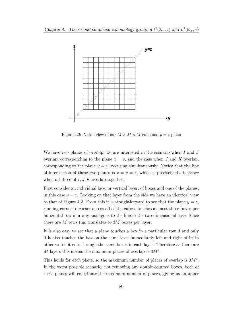
Chapter 4. The second simplicial cohomology group of `1(Z+, ∨) and L1(R+, ∨)
Figure 4.2: A side view of our M ×M ×M cube and y = z plane
We have two planes of overlap; we are interested in the scenario when I and J
overlap, corresponding to the plane x = y, and the case when J and K overlap,
corresponding to the plane y = z, occuring simultaneously. Notice that the line
of intersection of these two planes is x = y = z, which is precisely the instance
when all three of I, J,K overlap together.
First consider an individual face, or vertical layer, of boxes and one of the planes,
in this case y = z. Looking on that layer from the side we have an identical view
to that of Figure 4.2. From this it is straightforward to see that the plane y = z,
running corner to corner across all of the cubes, touches at most three boxes per
horizontal row in a way analagous to the line in the two-dimensional case. Since
there are M rows this translates to 3M boxes per layer.
It is also easy to see that a plane touches a box in a particular row if and only
if it also touches the box on the same level immediately left and right of it; in
other words it cuts through the same boxes in each layer. Therefore as there are
M layers this means the maximum places of overlap is 3M2.
This holds for each plane, so the maximum number of places of overlap is 3M2.
In the worst possible scenario, not removing any double-counted boxes, both of
these planes will contribute the maximum number of places, giving us an upper
80

Chapter 4. The second simplicial cohomology group of `1(Z+, ∨) and L1(R+, ∨)
bound of 6M2 for the total number of places of overlap.
So, proceeding as we did above, we divide the intervals on which I, J,K are
defined into M equal subintervals, obtaining
ϕ(I, J)(K) =M∑i=1
M∑j=1
M∑k=1
ϕ(Ii, Jj)(Kk), (4.102)
and this becomes
ϕ(I, J)(K) =∑
Ii∩Jj∩Kk=∅
ϕ(Ii, Jj)(Kk) +∑
Ii∩Jj∩Kk 6=∅
ϕ(Ii, Jj)(Kk)
=∑
Ii∩Jj∩Kk=∅
(δ2ψ)(Ii, Jj)(Kk) +∑
Ii∩Jj∩Kk 6=∅
ϕ(Ii, Jj)(Kk)
(as we can cobound ϕ by ψ when the intervals do not overlap)
=M∑
i,j,k=1
(δ2ψ)(Ii, Jj)(Kk)
+∑
Ii∩Jj∩Kk 6=∅
(ϕ(Ii, Jj)(Kk)− (δ2ψ)(Ii, Jj)(Kk)
)= (δ2ψ)(I, J)(K) +
∑Ii∩Jj∩Kk 6=∅
(ϕ(Ii, Jj)(Kk)− (δ2ψ)(Ii, Jj)(Kk)
).
(4.103)
The maximum number of places of overlap is 6M2 and so∣∣∣∣∣∣∑
Ii∩Jj∩Kk 6=∅
(ϕ(Ii, Jj)(Kk)− (δ2ψ)(Ii, Jj)(Kk)
)∣∣∣∣∣∣≤
∑Ii∩Jj∩Kk 6=∅
∣∣ϕ(Ii, Jj)(Kk)− (δ2ψ)(Ii, Jj)(Kk)∣∣
≤ 6M2 ·(‖ϕ‖ ‖Ii‖ ‖Jj‖ ‖Kk‖+
∥∥δ2ψ∥∥ ‖Ii‖ ‖Jj‖ ‖Kk‖
)= 6M2 ·
(‖ϕ‖ |I|
M
|J |M
|K|M
+∥∥δ2ψ
∥∥ |I|M
|J |M
|K|M
)−→ 0,
(4.104)
81

Chapter 4. The second simplicial cohomology group of `1(Z+, ∨) and L1(R+, ∨)
as M tends to ∞. Therefore we have that
ϕ(I, J)(K)
= limM→∞
(ϕ(I, J)(K))
= limM→∞
(δ2ψ)(I, J)(K) +∑
Ii∩Jj∩Kk 6=∅
(ϕ(Ii, Jj)(Kk)− (δ2ψ)(Ii, Jj)(Kk)
)= (δ2ψ)(I, J)(K) + lim
M→∞
∑Ii∩Jj∩Kk 6=∅
(ϕ(Ii, Jj)(Kk)− (δ2ψ)(Ii, Jj)(Kk)
)= (δ2ψ)(I, J)(K),
(4.105)
i.e.
ϕ(I, J)(K) = (δ2ψ)(I, J)(K). (4.106)
We are thus able to conclude that whether the intervals overlap or not we can
cobound our given ϕ with our chosen ψ. Even if the intervals are not defined in
any order, with arbitrary ways of overlapping, we can divide them up into partic-
ular smaller subintervals and the result follows from the linearity and properties
of both ϕ and δ2ψ.
It is necessary to check that ψ does indeed have all the desired properties, that is
it is bounded, linear and measurable. It is straightforward to do all of this from
first principles, but we can more easily just use the fact that ψ is defined using
ϕ, and so the result for ψ automatically follows from the same facts that are true
for ϕ.
We have shown that given a cyclic 2-cocycle ϕ ∈ ZC2(B) we can cobound it by
ψ ∈ C1(B,B∗), demonstrating that
HC2(B) = 0, (4.107)
the second cyclic cohomology group of B = L1(R+, ∨) is trivial.
Consider the section of the Connes-Tzygan long exact sequence given in Section
82

Chapter 4. The second simplicial cohomology group of `1(Z+, ∨) and L1(R+, ∨)
2.2.3 consisting of
· · · - HC2(B) - HH2(B) - HC1(B) - · · · .
We know that HC1(B) and HC2(B) are trivial and that the sequence is exact at
HH2(B) and so
HH2(B) = ker(HH2(B)→ 0) = im(0→ HH2(B)) = 0, (4.108)
i.e.
HH2(L1(R+, ∨)) = 0, (4.109)
and so we have shown that the second simplicial cohomology group for the algebra
B = L1(R+, ∨) is trivial.
4.3 An example of cobounding a particular
cyclic 2-cocycle
We may ask how a specific 2-cocycle cobounds. Let ϕ(f, g)(h) = τ(fgh), where
τ(k) =
∫ ∞0
k(t)dt. (4.110)
We can show this is a 2-cocycle by direct calculation, or we could simply observe
that in the Connes-Tzygan long exact sequence the map between HC0(B) into
HC2(B) takes the trace τ to the cyclic 2-cocycle ϕτ which is exactly our ϕ here.
From our analysis recall that ψ was chosen based on indicator functions I, J,K
as
ψ(I)(K) = ϕ(I, J)(K), (4.111)
where ϕ is independent of the middle term. Thus let
ψ(f)(g) = τ(fg). (4.112)
83
Chapter 4. The second simplicial cohomology group of `1(Z+, ∨) and L1(R+, ∨)
Then
(δ2ψ)(f, g)(h) = ψ(g)(h ∗ f)− ψ(f ∗ g)(h) + ψ(f)(g ∗ h)
= τ(gfh)− τ(fgh) + τ(fgh)
= τ(fgh)
= ϕ(f, g)(h),
(4.113)
and so ψ cobounds ϕ. This ψ is not cyclic, and since HC2(L1(R+, ∨)) = 0
it must be possible to cyclically cobound ϕ also where the requirement is for
ψ(f)(g) = −ψ(g)(f). On interval functions I and K we wrote ψ as
ψ(I)(K) =
∫ ∞0
∫ ∞0
Ψ(s, u)I(s)K(u)dsdu. (4.114)
For indicator functions I, J,K with order structure I � J � K it follows from
our analysis that
ϕ(I, J)(K) = τ(IJK)
=
∫ ∞0
(I ∗ J ∗K) (t)dt
=
∫ ∞0
K(t)dt = 1,
(4.115)
and so
ϕ(I, J)(K) = ψ(I)(K) =
∫ ∞0
∫ ∞0
Ψ(s, u)I(s)K(u)dsdu = 1. (4.116)
This rearranges to give
1
|I|1
|K|
∫ b0
a0
∫ b1
a1
Ψ(s, u)dsdu = 1, (4.117)
recalling that I is defined on [a1, b1] and K is defined on [a0, b0]. If we set
Ψ(s, u) =
1, s < t,
−1, s > t,(4.118)
84

Chapter 4. The second simplicial cohomology group of `1(Z+, ∨) and L1(R+, ∨)
we will recover what we want, i.e. that ψ is cyclic and it does indeed cobound ϕ for
indicator functions. What happens when s = u is of little interest as this occurs
on a line, an area of the plane which has Lebesgue measure zero; incidentally this
is precisely why the second cyclic cohomology group in the discrete case is not
trivial. This extends by linearity to general L1(R+, ∨) functions.
Thus we have proven that the second simplicial cohomology groups for the alge-
bras A = `1(Z+, ∨) and B = L1(R+, ∨) are both trivial.
4.4 An example of an algebra with nontrivial
second simplicial cohomology
One may be forgiven for thinking that our methods are applicable to any Banach
algebra spanned by idempotents and that therefore there must not be such a
Banach algebra with nontrivial second simplicial cohomology. The aim of this
section is to provide a counterexample to dispel this notion.
We consider the algebra A∞ = `1(N, ∨, µ) with measure on the underlying semi-
group given by µ({n}) = n. The key point of note here is that the measure is
unbounded on atoms, and is essentially a weighted algebra with weight w(n) = n.
The idea is to uniquely cobound a 2-cocycle ϕ ∈ Z2(A∞) by an unbounded ψ;
because ψ is unbounded it cannot be in C1(A∞, (A∞)∗) and hence is not an
element of B2(A∞), therefore making the second simplicial cohomology group of
A∞ nontrivial as required.
Let f ∈ A∞. Then f is a sequence, which in a way analogous to that for the
algebra `1(Z+, ∨) can be written as
f =∞∑i=1
fiδi, (4.119)
where fi ∈ C and δi is the indicator function
δi(n) =
1, n = i,
0, else,(4.120)
85
Chapter 4. The second simplicial cohomology group of `1(Z+, ∨) and L1(R+, ∨)
which are the generators of this algebra.
It also follows that the usual norm on this algebra is given by
‖f‖ =∞∑i=1
|fi|µc(i) =∞∑i=1
|fi| · i <∞. (4.121)
As we have done throughout this chapter let us assume that we are working with
f, g, h ∈ A∞ which are all normalised, that is have norm equal to 1.
Notation. For convenience let ψi,j = ψ(δi)(δj) and ϕi,j,k = ϕ(δi, δj)(δk).
It is once again sufficient by linearity arguments to define ψ and ϕ on the gener-
ators for A∞. We now define ψ : A∞ → (A∞)∗ to be
ψ(δi)(δj) =
0, i = j,
i2j, i < j,
−j2i, i > j.
(4.122)
It follows that ψi,j = −ψj,i and it is well-defined.
Then we have that
ϕi,j,k = (δ2ψ)(δi, δj)(δk)
= ψj,k∨i − ψi∨j,k + ψi,j∨k(4.123)
Because of the fact that ψi,j = −ψj,i and the indices i, j, k must occur in some
relative order in N we are able to arrive at the same conclusion regardless of the
actual ordering. Thus without loss of generality let us say that i ≤ j ≤ k. Then
ϕi,j,k = ψi,k. (4.124)
Going through the other orderings in turn will show us that in fact
ϕi,j,k = ψmin(i,j,k),max(i,j,k). (4.125)
86

Chapter 4. The second simplicial cohomology group of `1(Z+, ∨) and L1(R+, ∨)
It is straightforward to show that δ3ϕ = 0. It also follows that
‖ϕ‖ = sup‖f‖,‖g‖,‖h‖≤1
|ϕ(f, g)(h)|
= sup‖f‖,‖g‖,‖h‖≤1
∣∣∣∣∣∞∑
i,j,k=1
fi · gj · hk · (δ2ψ)(δi, δj)(δk)
∣∣∣∣∣= sup‖f‖,‖g‖,‖h‖≤1
∣∣∣∣∣∞∑
i,j,k=1
fi · i · gj · j · hk · k ·(δ2ψ)(δi, δj)(δk)
i · j · k
∣∣∣∣∣≤ sup‖f‖,‖g‖,‖h‖≤1
∞∑i,j,k=1
|fi| · i · |gj| · j|hk| · k ·|(δ2ψ)(δi, δj)(δk)|
i · j · k
(4.126)
Assume without loss of generality that i ≤ j ≤ k; of course any ordering will lead
to the same conclusion. Then
|(δ2ψ)(δi, δj)(δk)| = |ψik| = i2k. (4.127)
Also we have thati2k
i · j · k≤ sup
i,j,k∈N
(i2k
i · j · k
)< 1 (4.128)
as i ≤ j ≤ k. Hence
‖ϕ‖ ≤ sup‖f‖,‖g‖,‖h‖≤1
∞∑i,j,k=1
|fi| · i · |gj| · j|hk| · k · 1
= sup‖f‖,‖g‖,‖h‖≤1
(∞∑i=1
|fi| · i
)(∞∑j=1
|gj| · j
)(∞∑k=1
|hk| · k
)= sup‖f‖,‖g‖,‖h‖≤1
‖f‖ ‖g‖ ‖h‖
= 1,
(4.129)
i.e. ‖ϕ‖ ≤ 1 and so ϕ is bounded. Therefore we can conclude that ϕ = δ2ψ ∈Z2(A∞); i.e. ϕ is a 2-cocycle cobounded by ψ.
87

Chapter 4. The second simplicial cohomology group of `1(Z+, ∨) and L1(R+, ∨)
However, notice that following the same steps as before
‖ψ‖ = sup‖f‖,‖g‖≤1
|ψ(f)(g)|
≤ sup‖f‖,‖g‖≤1
∞∑i,j=1
|fi| · i · |gj| · j ·|ψi,j|i · j
.(4.130)
As we are still assuming that i ≤ j then it follows that |ψi,j| = i2j and thus
|ψi,j|i · j
=i2j
i · j≤ sup
i,j∈N(i) =∞, (4.131)
and hence
‖ψ‖ ≤ sup‖f‖,‖g‖≤1
∞∑i,j=1
|fi| · i · |gj| · j · ∞, (4.132)
and finally then ‖ψ‖ ≤ ∞.
It is not difficult to manufacture arguments to make ‖ψ‖ =∞. For consider the
functions f1 = 1xδx and g1 = 1
yδy with x, y ∈ N such that x < y. Then we have
that ‖f1‖ = ‖g1‖ = 1 and
‖ψ‖ = sup‖f‖,‖g‖≤1
|ψ(f)(g)|
≥ |ψ(f1)(g1)|
=
∣∣∣∣ψ(1
xδx)(
1
yδy)
∣∣∣∣=
1
xy|ψx,y|
=1
xy· x2y
= x.
(4.133)
Since x ∈ N was an arbitrary choice it must be that ‖ψ‖ ≥ x for all x ∈ N,
and therefore we conclude that ψ is unbounded. Thus ψ /∈ C1(A∞, (A∞)∗) and
therefore ψ /∈ B2(A∞), as required.
The final point to note here is that given ϕ ∈ Z2(A∞) it must cobound uniquely.
88

Chapter 4. The second simplicial cohomology group of `1(Z+, ∨) and L1(R+, ∨)
For if ψ1 and ψ2 are two coboundings of ϕ then it follows that
ϕ = δ2ψ1 = δ2ψ2 (4.134)
and thus δ2(ψ1 − ψ2) = 0, making ψ1 − ψ2 a derivation. As A∞ is spanned by
idempotents, namely the generators δi for i ∈ N, it follows from Theorem 3.1
that there are no nontrivial derivations on this algebra. Therefore ψ1 − ψ2 = 0
and hence
ψ1 = ψ2 (4.135)
and the cobounding is unique.
Hence we have proven the result we set out to show at the beginning of this
section, allowing us to finally say that HH2(A∞) is nontrivial, as required.
89
Chapter 5
The general simplicial
cohomology group of L1(R+,∨)
The main aim of this thesis is to obtain results about the nth simplicial cohomol-
ogy group for the semigroup algebra B = L1(R+, ∨). Having considered the first
and second simplicial cohomology groups for B we now generalise the methods
used in Chapters 3 and 4 in order to show that, for all n ∈ N, n ≥ 2,
HHn(B) = 0. (5.1)
When we try to adapt the methods found in Chapters 3 and 4 directly to higher
cohomology groups we run into problems. For instance the cocycle identities
no longer yield the same important information and it becomes very difficult
to perform any of the calculations required. These difficulties are compounded
further by the fact that the increasing dimensions vastly increases the number
of these calculations, their complexity and their length making such attempts
nearly impossible to compute by hand as we have been doing so far.
In order to overcome the above difficulties we sought inspiration from the discrete
case. The results are already known and we attempted to arrive at the same
conclusions via our methods.
However the main problem we will encounter is due to the inability to cobound
cocycles uniquely. For let ϕ be a cyclic 2-cocycle that is cobounded by both ψ1
90
Chapter 5. The general simplicial cohomology group of L1(R+, ∨)
and ψ2 in CC1(B). Then
ϕ = δ2ψ1 = δ2ψ2, (5.2)
and so we have δ2(ψ1 − ψ2) = 0, i.e. ψ1 − ψ2 ∈ ker(δ2). Since HC1(B) is trivial
we know ker(δ2) = im(δ1) and thus there exists χ ∈ B∗ such that
ψ1 − ψ2 = δ1χ. (5.3)
However
δ1χ(f1)(f0) = χ(f0 ∗ f1)− χ(f1 ∗ f0) (5.4)
for f1, f0 ∈ B, and by the commutativity of B this reduces to give δ1χ ≡ 0. This
holds for all χ ∈ B∗ and so
ψ1 − ψ2 = 0⇒ ψ1 = ψ2. (5.5)
This uniqueness of coboundary does not continue into higher dimensions. For
example consider ϕ to be a cyclic 3-cocycle. If ϕ is cobounded by ψ then it is
also cobounded by ψ + δ2χ for any χ ∈ CC1(B). Then δ2χ ∈ im(δ2), which
is BC2(B). This space is not trivial and so it does not necessarily follow that
δ2χ = 0, meaning that our cyclic 3-cocycle could indeed be cobounded by several
candidates.
This makes searching for coboundings directly much more problematic in higher
dimensions as there is no route to the solution. Previously we stated that if we
could cobound a cocycle ϕ by ψ then ψ had to exhibit certain properties which
helped us to identify it precisely. This method no longer yields fruitful results
when the solution is not unique; as there is almost no unique cobounding then it
is harder to pick a particular choice of coboundary.
Therefore it has become necessary to adopt a more abstract method for proving
the triviality of the nth simplicial cohomology group of B.
At the start of this chapter we use the method of Section 4.2 to guide us in
formulating a more general and abstract method in order to obtain the same
result for HH2(B). The rest of the chapter is dedicated to applying this method
to the nth case.
91

Chapter 5. The general simplicial cohomology group of L1(R+, ∨)
5.1 Re-evaluating the second simplicial
cohomology group
In this section we will re-evaluate the second simplicial cohomology group case
from Section 4.2 and produce a more direct method for proving its triviality.
The general strategy that we shall adopt to do this will begin with a result about
the cobounding of a 2-cocycle that is defined on arguments which are L1 functions
where the supports of these functions are ordered and disjoint such that the first
term has support to the left of the second term which in turn has support to the
left of the final term. Then we extend this cobounding via several interesting
methods, first to other distinct orderings and then to the general case using some
results concerned with the rewriting and approximating of the general case as
a linear combination of the various ordered cases. Finally, having shown that
these coboundings occur and the general case can be approximated by this, we
will have shown that the second simplicial cohomology group for this semigroup
algebra is trivial.
5.1.1 Cobounding a 2-cocycle on a particular ordering of
arguments
Let ϕ ∈ Z2(B) be a 2-cocycle. This section proves the following theorem:
Theorem 5.1. Let I1, I2, I0 be normalised indicator functions in B such that
I1 � I2 � I0. Then there exists ψ ∈ C1(B) such that
ϕ(I1, I2)(I0) = (δ2ψ)(I1, I2)(I0). (5.6)
In Section 4.2 the idea was to cobound a general ϕ ∈ ZC2(B) with a ψ ∈ CC1(B)
defined using the cyclic 2-cocyle we started with. We showed that it was sufficient
to prove the result only for normalised indicator functions and that these functions
could always be ordered as arguments of ϕ such that the first one listed was the
smallest, the last the largest and the second term between these in order.
Section 4.2 then went on to show that ϕ was independent of this second term
and so given ϕ(I1, I2)(I0) where the Ii are normalised indicator functions for
92

Chapter 5. The general simplicial cohomology group of L1(R+, ∨)
i = 0, 1, 2, we replaced I2 with a normalised indicator function defined on the
largest possible support that lay between the supports of I1 and I0. We then used
this to define our ψ and showed that this cobounded ϕ(I1, I2)(I0).
A version of this theorem has been proven in Section 4.2 in the cyclic case. We
now prove it for the general case.
Recall that it is possible to write ϕ ∈ Z2(B) and ψ ∈ C1(B) as
ϕ(I1, I2)(I0) =
∫R3
+
Φ(x1, x2, x0)I1(x1)I2(x2)I0(x0)dx1dx2dx0,
ψ(I1)(I0) =
∫R2
+
Ψ(x1, x0)I1(x1)I0(x0)dx1dx0,
(5.7)
respectively, where Φ ∈ L∞(R3+) and Ψ ∈ L∞(R2
+).
Before giving the proof of Theorem (5.1) we need the following two results.
Lemma 5.1. Let ϕ be as above with I1 � I2 � I3 � I0 normalised indicator
functions in B. Then∫R4
+
Φ(x1, x3, x0)I1(x1)I2(x2)I3(x3)I0(x0)dx1dx2dx3dx0
=
∫R4
+
Φ(x1, x2, x0)I1(x1)I2(x2)I3(x3)I0(x0)dx1dx2dx3dx0. (5.8)
Proof. The cocycle identity gives us that
0 = (δ3ϕ)(I1, I2, I3)(I0)
= ϕ(I2, I3)(I0 ∗ I1)− ϕ(I1 ∗ I2, I3)(I0) + ϕ(I1, I2 ∗ I3)(I0)− ϕ(I1, I2)(I3 ∗ I0)
= ϕ(I2, I3)(I0)− ϕ(I2, I3)(I0) + ϕ(I1, I3)(I0)− ϕ(I1, I2)(I0),
(5.9)
which rearranges to give
ϕ(I1, I3)(I0) = ϕ(I1, I2)(I0). (5.10)
93
Chapter 5. The general simplicial cohomology group of L1(R+, ∨)
Using the rewritten versions above this becomes∫R3
+
Φ(x1, x3, x0)I1(x1)I3(x3)I0(x0)dx1dx3dx0
=
∫R3
+
Φ(x1, x2, x0)I1(x1)I2(x2)I0(x0)dx1dx2dx0. (5.11)
Now notice that ∫R+
Ii(x)dxi = 1, i = 0, 1, 2, 3 (5.12)
and so the above equation becomes
1×∫
R3+
Φ(x1, x3, x0)I1(x1)I3(x3)I0(x0)dx1dx3dx0
= 1×∫
R3+
Φ(x1, x2, x0)I1(x1)I2(x2)I0(x0)dx1dx2dx0
⇒∫
R4+
Φ(x1, x3, x0)I1(x1)I2(x2)I3(x3)I0(x0)dx1dx2dx3dx0
=
∫R4
+
Φ(x1, x2, x0)I1(x1)I2(x2)I3(x3)I0(x0)dx1dx2dx3dx0,
(5.13)
as required.
Lemma 5.2. Let I0, I1, I2 be normalised indicator functions in B such that I1 �I2 � I0. Then
ϕ(I1, I2)(I0) = ϕ(I1, I0)(I2). (5.14)
Proof. Choose I3 ∈ B such that I1 � I3 � I2; such a choice can always be made
given the disjoint nature of the supports of I1 and I2. Using these the cocycle
identity gives us
0 = (δ3ϕ)(I1, I3, I0)(I2)
= ϕ(I3, I0)(I2)− ϕ(I3, I0)(I2) + ϕ(I1, I0)(I2)− ϕ(I1, I3)(I0),(5.15)
which becomes
ϕ(I1, I0)(I2) = ϕ(I1, I3)(I0). (5.16)
94

Chapter 5. The general simplicial cohomology group of L1(R+, ∨)
By Lemma (5.1) it follows that ϕ(I1, I3)(I0) = ϕ(I1, I2)(I0), and so
ϕ(I1, I0)(I2) = ϕ(I1, I2)(I0), (5.17)
as required.
This result can be extended to the case with a non-normalised function f instead
of I2 such that the support of f lies entirely in the order structure between the
supports of I1 and I0 by linearity. For approximate f by a linear combination of
disjoint normalised indicator functions Jj. Note that each Jj for j = 0, 1, . . . has
support between those of I1 and I0 also. Then we have, where αj ∈ C for j ∈ Z+,
ϕ(I1, f)(I0) =∞∑j=0
αjϕ(I1, Jj)(I0)
=∞∑j=0
αjϕ(I1, I0)(Jj)
= ϕ(I1, I0)(f).
(5.18)
We can also extend the result of Lemma (5.1) to such an f . For the cocycle
identity on normalised indicator functions I1 � I2 � I0 with f fitting within the
order structure such that its support is between the supports of I2 and I0 gives
us
0 = (δ3ϕ)(I1, I2, f)(I0) = ϕ(I2, f)(I0)− ϕ(I2, f)(I0) + ϕ(I1, f)(I0)
− ϕ(I1, I2)(ϑ(f)I0)(5.19)
as it can easily be shown that (I2 ∗ f)(x) = f(x) and (f ∗ I0)(x) = ϑ(f)I0, where
ϑ is the augmentation character defined by
ϑ(f) =
∫ ∞0
f(x)dx = f(∞) (5.20)
for f ∈ L1(B). Thus
ϕ(I1, f)(I0) = ϑ(f)ϕ(I1, I2)(I0). (5.21)
95

Chapter 5. The general simplicial cohomology group of L1(R+, ∨)
If f is positive and normalised then this result is even simpler as ϑ(f) = 1.
Remark. The result from Lemma (5.1) states that for the ordering I1 � I2 �I3 � I0 we have
ϕ(I1, I2)(I0) = ϕ(I1, I3)(I0). (5.22)
However this is not as restrictive as it seems; we can replace the middle term by
any normalised indicator function with support disjoint from and between the
supports of I1 and I0. For consider I such that I1 � I � I0. Note that we
make no restriction on the relation between I and I2; it may be that I ∩ I2 6= ∅.Begin with ϕ(I1, I2)(I0) and note that we can always find a normalised indicator
function I3 such that both I2 � I3 � I0, I � I3 � I0 hold. Then by Lemma
(5.1) it follows that
ϕ(I1, I2)(I0) = ϕ(I1, I3)(I0) = ϕ(I1, I)(I0). (5.23)
We are now in a position to give the proof of Theorem (5.1).
Proof. [Theorem (5.1)] As in Chapter 4 we set
Ψ(x1, x0) =
∫ x0
x1
Φ(x1, t, x0)
x0 − x1
dt, x1 < x0,
0, else.
(5.24)
Then if ψ is to cobound ϕ it must be that
ϕ(I1, I2)(I0) = (δ2ψ)(I1, I2)(I0)
= ψ(I2)(I0 ∗ I1)− ψ(I1 ∗ I2)(I0) + ψ(I1)(I2 ∗ I0)
= ψ(I2)(I0)− ψ(I2)(I0) + ψ(I1)(I0)
= ψ(I1)(I0),
(5.25)
i.e. that ψ(I1)(I0) = ϕ(I1, I2)(I0). Therefore we are required to show that∫R2
+
Ψ(x1, x0)I1(x1)I0(x0)dx1dx0 =
∫R3
+
Φ(x1, x2, x0)I1(x1)I2(x2)I0(x0)dx1dx2dx0,
(5.26)
96
Chapter 5. The general simplicial cohomology group of L1(R+, ∨)
which after making the substitution for Ψ becomes∫R2
+
∫ x0
x1
Φ(x1, t, x0)
x0 − x1
dtI1(x1)I0(x0)dx1dx0
=
∫R3
+
Φ(x1, x2, x0)I1(x1)I2(x2)I0(x0)dx1dx2dx0. (5.27)
Looking at the left hand side this becomes∫R2
+
∫R+
Φ(x1, t, x0)I[x1,x0)(t)
x0 − x1
dtI1(x1)I0(x0)dx1dx0
=
∫R3
+
Φ(x1, t, x0)
[I[x1,x0)(t)
x0 − x1
(χ[x2,∞)(t) + χ[0,x2)(t)
)]dtI1(x1)I0(x0)dx1dx0
=
∫R3
+
Φ(x1, t, x0)
[I[x1,x0)(t)
x0 − x1
× χ[x2,∞)(t)
]dtI1(x1)I0(x0)dx1dx0
+
∫R3
+
Φ(x1, t, x0)
[I[x1,x0)(t)
x0 − x1
× χ[0,x2)(t)
]dtI1(x1)I0(x0)dx1dx0,
(5.28)
where χ[x2,∞)(t) and χ[0,x2)(t) are the characteristic functions (not necessarily
normalised) defined on the supports [x2,∞) and [0, x2) respectively.
A little thought makes it clear that
I[x1,x0)(t)
x0 − x1
× χ[x2,∞)(t) =I[x2,x0)(t)
x0 − x1
,
I[x1,x0)(t)
x0 − x1
× χ[0,x2)(t) =I[x1,x2)(t)
x0 − x1
,
(5.29)
and so the equation in (5.28) then becomes∫R3
+
Φ(x1, t, x0)I[x2,x0)(t)
x0 − x1
dtI1(x1)I0(x0)dx1dx0
+
∫R3
+
Φ(x1, t, x0)I[x1,x2)(t)
x0 − x1
dtI1(x1)I0(x0)dx1dx0. (5.30)
Note that ∫R+
I2(x2)dx2 = 1 (5.31)
97

Chapter 5. The general simplicial cohomology group of L1(R+, ∨)
by construction, and so it follows that equation (5.30) becomes∫R4
+
Φ(x1, t, x0)I[x2,x0)(t)
x0 − x1
dtI1(x1)I2(x2)I0(x0)dx1dx2dx0
+
∫R4
+
Φ(x1, t, x0)I[x1,x2)(t)
x0 − x1
dtI1(x1)I2(x2)I0(x0)dx1dx2dx0. (5.32)
We then appeal to Lemma (5.1) to yield∫R4
+
Φ(x1, x2, x0)I[x2,x0)(t)
x0 − x1
dtI1(x1)I2(x2)I0(x0)dx1dx2dx0
+
∫R4
+
Φ(x1, x2, x0)I[x1,x2)(t)
x0 − x1
dtI1(x1)I2(x2)I0(x0)dx1dx2dx0. (5.33)
This in turn reduces to∫R3
+
Φ(x1, x2, x0)
[x0 − x2 + x2 − x1
x0 − x1
]I1(x1)I2(x2)I0(x0)dx1dx2dx0 (5.34)
which is simply∫R3
+
Φ(x1, x2, x0)I1(x1)I2(x2)I0(x0)dx1dx2dx0 = ϕ(I1, I2)(I0), (5.35)
as required.
This shows that for the order structure I1 � I2 � I0 we can approximate these
functions by normalised indicator functions and by setting
ψ(I1)(I0) = ϕ(I1, I[a,b])(I0) (5.36)
for I[a,b] with the largest possible support between those of I1 and I0 and still
disjoint will yield a cobounding of ϕ(I1, I2)(I0) in this case. However we require
this result to be extended to other possible orderings of the disjoint supports of
the normalised functions Ii; doing so by this method is possible but very difficult.
The difficulty lies in proving that the choice of a similar ψ for our given 2-cocycle
ϕ defined on the case where the supports of I1, I2, I0 are decreasing disjoint is
well-defined. It requires an analogue of Lemma (5.1) (where the orders are all
98
Chapter 5. The general simplicial cohomology group of L1(R+, ∨)
reversed), which is difficult if not impossible to prove.
Thus we are forced at this point to amend the method we have created so far. The
difficulty lies primarily in the notion of using the normalised indicator function of
largest support between those of I1 and I0 to define ψ using ϕ as it is not always
clear to see if this is well-defined. This suggests that the logical way forward is to
somehow invoke the use of the normalised indicator function of smallest support
between those of I1 and I0 instead, in a sense to be explained later.
An alternative approach
It is convenient at this point to introduce a change in approach to the definitions
of ϕ and ψ also. First define
ϕ ((I1, I2, I0)) = ϕ(I1, I2)(I0), (5.37)
which is a bounded multilinear map from L1(R+, ∨)×L1(R+, ∨)×L1(R+, ∨) into
C. Then this multilinear map on L1(R+, ∨) × L1(R+, ∨) × L1(R+, ∨) defines a
linear map on the tensor product space L1(R+, ∨)⊗L1(R+, ∨)⊗L1(R+, ∨) in the
usual manner by the fact this is isometrically isomorphic to L1(R3+); we denote
such a linear map by ϕ. So
ϕ(I1, I2)(I0) = ϕ ((I1, I2, I0)) = ϕ(I1 ⊗ I2 ⊗ I0). (5.38)
Similarly,
ψ(I1)(I0) = ψ ((I1, I0)) = ψ(I1 ⊗ I0). (5.39)
It is now more convenient to work with ϕ and ψ.
Definition. Let the function εk : B→ B⊗B ∼= L1(R2+, ∨) be defined for Ii ∈ B
with i ∈ Z+ by the formula
εk(Ii)(x, y) = εk,x(Ii)(y) = Ii(y)χ[0, 1
k)(y − x)(
1k
) = k · Ii(y) · χ[x,x+ 1k)(y). (5.40)
We call εk the left spreading out function.
99
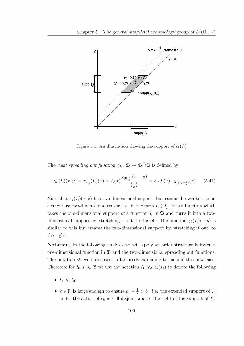
Chapter 5. The general simplicial cohomology group of L1(R+, ∨)
Figure 5.1: An illustration showing the support of εk(Ii)
The right spreading out function γk : B→ B⊗B is defined by
γk(Ii)(x, y) = γk,y(Ii)(x) = Ii(x)χ[0, 1
k)(x− y)(
1k
) = k · Ii(x) · χ[y,y+ 1k)(x). (5.41)
Note that εk(Ii)(x, y) has two-dimensional support but cannot be written as an
elementary two-dimensional tensor, i.e. in the form Ii⊗ Ij. It is a function which
takes the one-dimensional support of a function Ii in B and turns it into a two-
dimensional support by ‘stretching it out’ to the left. The function γk(Ii)(x, y) is
similar to this but creates the two-dimensional support by ‘stretching it out’ to
the right.
Notation. In the following analysis we will apply an order structure between a
one-dimensional function in B and the two-dimensional spreading out functions.
The notation � we have used so far needs extending to include this new case.
Therefore for I0, I1 ∈ B we use the notation I1 �k εk(I0) to denote the following
• I1 � I0;
• k ∈ N is large enough to ensure a0− 1k> b1, i.e. the extended support of I0
under the action of εk is still disjoint and to the right of the support of I1.
100

Chapter 5. The general simplicial cohomology group of L1(R+, ∨)
Figure 5.2: An illustration showing the support of γk(Ii)
This last also implies that εk(I0) ∩ I1 = ∅. This set up merely says that the
supports of I0 and I1 are ordered with I1 being the smallest, and the left spreading
out function does not spread the support of I0 as far to the left so as to intercept
the support of I1.
A very similar definition applies to I1 �k γk(I0).
Remark. Note that in order for a similar situation to be applied to the expression
εk(I1)�k I0 (sim. γk(I0)�k I1) it is only necessary to impose the condition that
I0 � I1; there is no dependence on k in order to preserve disjointed order between
the two-dimensional support of εk(I0) (sim. γk(I0)) and the one-dimensional
support of I1. Hence we drop the subscript k on the order relation and simply
say that εk(I0)� I1 (sim. γk(I0)� I1) here.
This is illustrated in Figures (5.3) and (5.4), which show the necessity of demand-
ing k to be large enough in order to ensure a disjoint separation of supports.
101

Chapter 5. The general simplicial cohomology group of L1(R+, ∨)
Figure 5.3: An illustration of the relations I1 �k εk(I0) (left) and εk(I0)� I1 (right).
Figure 5.4: An illustration of the relations I1 �k γk(I0) (left) and γk(I0)� I1 (right).
Approximations by elementary tensor products of normalised functions
Before we continue it is necessary for us to prove a particularly useful result. In
order to get to this however we will need the following lemma.
Lemma 5.3. Given F ∈ L1(R2+) there exists fi, gi ∈ L1(R+) with αi ∈ C for
i ∈ N such that
F (x, y) =∞∑i=1
αifi ⊗ gi, (5.42)
102

Chapter 5. The general simplicial cohomology group of L1(R+, ∨)
with∞∑i=1
|αi| <∞, ‖fi‖ = ‖gi‖ = 1.
The proof of this Lemma is a mixture of Example (14) and Proposition (12) in
§42 of [5]. First of all there is the existence of a linear isometric isomorphism
of L1(R+)⊗L1(R+) onto L1(R2+). For by the (universal) properties of tensor
products there exists a unique linear mapping T : L1(R+)⊗L1(R+) → L1(R2+)
such that
T (f ⊗ g)(x, y) = f(x)g(y), x, y ∈ R+, f, g ∈ L1(R+). (5.43)
Then it is observed that L1(R+)⊗L1(R+) can be represented as the linear sub-
space of BL2(L1(R+)∗;C) consisting of all elements of the form
u =∞∑n=1
fn ⊗ gn, (5.44)
where∞∑n=1
‖fn‖ ‖gn‖ <∞.
The result we are aiming at in this section is an extension of this lemma. Before
giving the result we need to define our objects of interest.
Definition. Recall that L1(R+)⊗L1(R+)⊗L1(R+) is isometrically isomorphic to
L1(R3+). Let W be the permutation group of the three elements x0, x1, x2. Then
for w ∈ W we define the wedge
Qw ={
(x1, x2, x0) ∈ R3+ : x1, x2, x0 satisfy the order structure given by w
}.
(5.45)
For example, if w1 = (x1, x2, x0) then
Qw1 ={
(x1, x2, x0) ∈ R3+ : 0 < x1 < x2 < x0
}. (5.46)
Then for w ∈ W we are able to define the quadrant L1(Qw) as a subspace of
L1(R3+) such that F ∈ L1(Qw) has support on the wedge Qw.
We are now ready to give the following result, which will allow us to write
103

Chapter 5. The general simplicial cohomology group of L1(R+, ∨)
F ∈ L1(Qw) as a linear combination of elementary tensor products of disjoint
normalised functions.
Lemma 5.4. Given F ∈ L1(Qw), where w ∈ W , F can be written as
∞∑i=1
αif(i)1 ⊗ f
(i)2 ⊗ f
(i)0 , (5.47)
where αi ∈ C,∞∑i=1
|αi| <∞, f(i)1 , f
(i)2 , f
(i)0 are normalised L1(B) functions for all
i ∈ N, and for each i the supports of these functions occur in the disjoint order
defined by the permutation w.
Proof. Without loss of generality we simply consider the two-dimensional case
and let L1(Q) to be the quadrant where functions are defined on the wedge
{(x1, x0) ∈ R2+ : x0 < x1}.
Define the following:
Rm = {(x1, x0) : x1 > x0 and m− 1 ≤ x1 < m},
Ikn,m =
[(m− 1) +
2k − 1
2n+1, (m− 1) +
2k
2n+1
),
Jkn,m =
[(m− 1) +
2k − 2
2n+1, (m− 1) +
2k − 1
2n+1
),
(5.48)
where k = 1, . . . , 2n, m ∈ N and n = 0, 1, . . .. This is represented pictorially in
Figures 5.5 and 5.6.
Then it follows that
R1 =∞⋃n=0
(2n⋃k=1
Ikn,1 × Jkn,1
), (5.49)
and for m ≥ 2
Rm =
[∞⋃n=0
(2n⋃k=1
Ikn,m × Jkn,m
)]∪ [[m− 1,m)× [0,m)] . (5.50)
Thus each Rm is a countable union of countable boxes. Since Q =∞⋃m=1
Rm, it
follows that Q is countable union of the segments Rm and so is a countable union
104

Chapter 5. The general simplicial cohomology group of L1(R+, ∨)
Figure 5.5: An illustration of the regions Rm for m = 1, 2, . . .
Figure 5.6: An illustration of splitting R1 into boxes Ikn,1 for n = 0, 1, . . . and k =1, . . . , 2n
105

Chapter 5. The general simplicial cohomology group of L1(R+, ∨)
of a countable union of countable boxes. Hence the region {(x1, x0) : x0 < x1}is itself also a countable union of boxes. Label each of these boxes in turn as
X1, X2, . . . ,, so that
{(x1, x0) : x0 < x1} =∞⋃x=1
Xx. (5.51)
Given F ∈ L1(Q) it follows that F (x1, x0) is equivalent to∞∑x=1
F · χXx
. For
notational convenience, relabel F ·χXx
as Fx. Each Fx is defined on a box, and so
is an element of L1(R2+), and it follows that Fx is zero outside of the box which
defines its support. Thus by Lemma (5.3) Fx can be written as
Fx =∞∑y=1
αyf(y)1 ⊗ f
(y)0 , (5.52)
with αy ∈ C,∞∑y=1
|αy| <∞ and∥∥∥f (y)
i
∥∥∥ = 1 for i = 0, 1 and y ∈ N. Notice that by
the nature of the wedge we are in it must follow that f0 � f1. Then
F (x1, x0) =∞∑x=1
∞∑y=1
αyf(y)1 ⊗ f
(y)0 . (5.53)
This is a countable sum of a countable sum and so is itself (trivially) a countable
sum. As such, relabel the terms in turn and index them by i to yield
F (x1, x0) =∞∑i=1
αif(i)1 ⊗ f
(i)0 , (5.54)
and hence proving the result as required.
It is clear after a little thought that this result extends to n dimensions, making
this a useful tool for the higher-order cohomology groups we shall consider later.
The left and right spreading out functions
We now give some results regarding the left and right spreading-out functions.
First we explore an inverse to both εk and γk before investigating the results of
106
Chapter 5. The general simplicial cohomology group of L1(R+, ∨)
convolving I1 in one variable with the 2-dimensional tensors εk(I0) and γk(I0),
where I1, I0 are normalised indicator functions.
Lemma 5.5. Let F ∈ B⊗B and Ii ∈ B. Let πk : B⊗B → B be the function
defined by
πk(F )(x) =
∫ x
0
F (t, x)dt+
∫ x
0
F (x, t)dt. (5.55)
Then πk is a left inverse to both εk and γk, that is to say πk(εk(Ii))(x) = Ii(x)
and πk(γk(Ii))(x) = Ii(x).
Proof. We only offer the proof for εk here; the proof for γk is very similar and
can be deduced from the following method.
Calculating the value of πk ◦ εk on Ii it follows that
πk(εk(Ii))(x) =
∫ x
0
εk(Ii)(t, x)dt+
∫ x
0
εk(Ii)(x, t)dt
=
∫ x
0
Ii(x) · k · χ[0, 1k)(x− t)dt+
∫ x
0
Ii(t) · k · χ[0, 1k)(t− x)dt.
(5.56)
The second term here reduces to zero as the range of the integral does not include
the support of χ[0, 1k)(t− x), so
πk(εk(Ii))(x) = Ii(x) · k∫ x
0
χ[0, 1k)(x− t)dt
= Ii(x) · k · 1
k= Ii(x).
(5.57)
A natural question which arises now concerns what happens when a function in
one variable Ii ∈ B is convolved with a two-dimensional function F ∈ B⊗B.
The natural module action of B on B⊗B defines left and right multiplication as
(Ii ∗ F )(x, y) =
∫ x
0
Ii(t)dt · F (x, y) + Ii(x) ·∫ x
0
F (t, y)dt (5.58)
and
(F ∗ Ii)(x, y) =
∫ y
0
F (x, t)dt · Ii(y) + F (x, y) ·∫ y
0
Ii(t)dt (5.59)
107

Chapter 5. The general simplicial cohomology group of L1(R+, ∨)
respectively. This ensures that for F = Ij⊗Ik we have Ii ∗(Ij⊗Ik) = (Ii ∗Ij)⊗Ikand (Ij ⊗ Ik) ∗ Ii = Ij ⊗ (Ik ∗ Ii) as expected.
Lemma 5.6. Let I0, I1 ∈ B and let k ∈ N be large enough to ensure that that
I1 �k εk(I0). Then
(I1 ∗ εk(I0))(x, y) = εk(I0)(x, y) = (εk(I0) ∗ I1)(x, y). (5.60)
The necessity of proving both cases is due to the lack of commutativity regarding
the product of a 1-dimensional tensor with a 2-dimensional tensor.
Proof. Again simply calculating the value of I1 ∗ εk(I0) on x, y yields
(I1 ∗ εk(I0))(x, y) =
∫ x
0
I1(t)dt · εk(I0)(x, y) + I1(x) ·∫ x
0
εk(I0)(t, y)dt
=
∫ x
0
I1(t)dt · I0(y) · k · χ[0, 1k)(y − x)
+ I1(x) · k∫ x
0
I0(y)χ[0, 1k)(y − t)dt.
(5.61)
If x /∈ (y − 1k, y] then this whole expression reduces to zero. This is because
χ[0, 1k)(y − x) = 0 in the first term. If furthermore x is not in the support of I1
then the second term is zero. If x does fall into the support of I1 then y − t > 1k
for all t ∈ [0, x] as I1 � I0 and y is in the support of I0.
If on the other hand x ∈ (y − 1k, y] then we have that x is not in the support of
I1 and so the second term is zero, leaving us with
(I1 ∗ εk(I0))(x, y) =
∫ x
0
I1(t)dt · I0(y) · k · χ[0, 1k)(y − x)
= 1 · I0(y) · k · χ[0, 1k)(y − x) = εk(I0)(x, y).
(5.62)
Thus we are able to conclude that
(I1 ∗ εk(I0))(x, y) = εk(I0)(x, y) (5.63)
as εk(I0)(x, y) = 0 if x /∈ (y − 1k, y] as required.
108
Chapter 5. The general simplicial cohomology group of L1(R+, ∨)
For the other case the multiplication yields
(εk(I0) ∗ I1)(x, y) =
∫ y
0
εk(I0)(x, t)dt · I1(y) + εk(I0)(x, y) ·∫ y
0
I1(t)dt
= kI1(y)
∫ y
0
I0(t)χ[x,x+ 1k)(t)dt+ kI0(y)χ[x,x+ 1
k)(y)
∫ y
0
I1(t)dt.
(5.64)
For this to be nontrivial we require that y is in the support of either I1 or I0;
obviously it cannot be in both as they are ordered and disjoint.
If y is in the support of I1 then the integral in the first term is zero while I0(y) = 0
in the second term, returning an overall trivial solution.
Thus if y is in the support of I0 the first term is zero while the second term
becomes
kI0(y)χ[x,x+ 1k)(y) · 1 = εk(I0)(x, y), (5.65)
proving the second case as required.
The results of these multiplications are quite different when the order structure
of I0 and I1 are reversed.
Proposition 5.1. Let I0, I1 ∈ B be normalised indicator functions such that
I0 � I1. Then
(I1 ∗ εk(I0))(x, y) = I1(x)I0(y) (5.66)
and
(εk(I0) ∗ I1)(x, y) = I1(y)f(x), (5.67)
where
f(x) =
0, x /∈ (a0 − 1k, b0),
(x−a0)k+1b0−a0
, x ∈ (a0 − 1k, a0],
1b0−a0
, x ∈ (a0, b0 − 1k],
k(b0−x)b0−a0
, (b0 − 1k, b0].
(5.68)
Proof. Case 1: I1 ∗ εk(I0)
109
Chapter 5. The general simplicial cohomology group of L1(R+, ∨)
Calculating the value of I1 ∗ εk on I0 we have that
(I1 ∗ εk(I0))(x, y) =
∫ x
0
I1(t)dt · εk(I0)(x, y) + I1(x) ·∫ x
0
εk(I0)(t, y)dt
= k · I0(y)χ[x,x+ 1k)(y)
∫ x
0
I1(t)dt
+ k · I1(x) · I0(y)
∫ x
0
χ[0, 1k)(y − t)dt.
(5.69)
In order for this to be nontrivial we need y to be in the support of I0.
If x /∈ (y− 1k, y] then the first term is zero as χ[x,x+ 1
k)(y) = 0. There are now two
possibilities for where x can be. If x is not in the support of I1 then the second
term is also trivial. On the other hand if x is in the support of I1 then the range
of the integral in the second term covers the whole of the support of χ[0, 1k)(y− t),
and thus this term becomes
k · I1(x) · I0(y) · 1
k= I1(x)I0(y). (5.70)
Alternatively if x ∈ (y − 1k, y] then it follows that x ≤ y. Thus as y is in the
support of I0 and I0 � I1 it follows that x is not in the support of I1. This
makes the integral in the first term and I1(x) in the second term both equal to
0, making the entire expression trivial.
The conditions and definitions of this expression allow us to conclude that
(I1 ∗ εk(I0))(x, y) = I1(x)I0(y) (5.71)
as required.
Case 2: εk(I0) ∗ I1
110
Chapter 5. The general simplicial cohomology group of L1(R+, ∨)
This case is a lot trickier. In calculating εk(I0) ∗ I1 on I0 we simply get
(εk(I0) ∗ I1)(x, y) =
∫ y
0
εk(I0)(x, t)dt · I1(y) + εk(I0)(x, y) ·∫y0I1(t)dt
= k · I1(y)
∫ y
0
I0(t)χ[0, 1k)(t− x)dt
+ k · I0(y) · χ[0, 1k)(y − x)
∫ y
0
I1(t)dt.
(5.72)
In order for this to be nontrivial we again require that y is in the support of
either I0 or I1; obviously it cannot be in both as their supports are ordered and
disjoint.
If y is in the support of I0 then I1(y) in the first term and the integral in the
second term are both zero, making the overall result trivial; the integral is zero
because the range of the integral is not large enough to reach the support of I1.
On the other hand if y is in the support of I1 then the second term is zero as
I0(y) = 0. The first term however simply becomes
k · I1(y)
∫ y
0
I0(t)χ[0, 1k)(t− x)dt = k · I1(y) ·
∫ b0
a0
1
b0 − a0
· χ[x,x+ 1k)(t)dt (5.73)
as [a0, b0] ⊂ [0, y] and I0(t) = 0 for all t /∈ [a0, b0] and using the definition of I0
on [a0, b0].
It is immediately clear after a little thought that χ[x,x+ 1k)(t) = 0 for all x /∈
(a0 − 1k, b0].
When x ∈ (a0 − 1k, a0] then the overlap between the support of the function
χ[x,x+ 1k)(t) and the range of the integral [a0, b0] is x + 1
k− a0. This makes the
integral simply the area of the box with height one and width (x + 1k− a0) and
hence the expression becomes
k · I1(y) · 1
b0 − a0
· (x+1
k− a0) = I1(y) · (x− a0)k + 1
b0 − a0
. (5.74)
When x ∈ (a0, b0 − 1k] the whole support of the function χ[x,x+ 1
k)(t) is contained
within the range of the integral. Thus the integral is the area under the whole of
111

Chapter 5. The general simplicial cohomology group of L1(R+, ∨)
χ[x,x+ 1k)(t), which is 1
kand the expression becomes
k · I1(y) · 1
b0 − a0
· 1
k= I1(y) · 1
b0 − a0
. (5.75)
Finally if x ∈ (b0 − 1k, b0] then the amount of overlap between the range of the
integral [a0, b0] and the support of the function χ[x,x+ 1k)(t) is (b0 − x). Then the
integral is simply the area of the box of height one and width (b0 − x), making
the expression become
k · I1(y) · 1
b0 − a0
· (b0 − x) = I1(y) · k(b0 − x)
b0 − a0
. (5.76)
Putting all of these together yields the second case of the proposition, as required.
Proposition (5.1) essentially shows that both (I1 ∗ εk(I0))(x, y) = I1(x)I0(y) and
(εk(I0) ∗ I1)(x, y) = I1(y)f(x) are 2-dimensional elementary tensor products.
In the first case this is simply I1 ⊗ I0 with order structure I0 � I1.
The second one is the one which will appear in our future calculations. Here the
tensor product is I1 ⊗ f , but f is not a normalised indicator function. Notice
though that the support of f is disjoint from and entirely below the support of
I1. Also f is defined on an interval (a0− 1k, b0] and it is normalised; we leave this
last as an exercise. We are also able to approximate this by a linear combination
of normalised indicator functions
f(x) =∞∑j=0
αjJj(x), (5.77)
such that Jj(x) � I1 for all j such that 0 ≤ j < ∞, with αj ∈ C. Then for
I2 � I0 � I1 and I2 �k εk(I0) we have that
ϕ(I2 ⊗ εk(I0) ∗ I1) =∞∑j=0
αjϕ(I2 ⊗ I1 ⊗ Jj)
=∞∑j=0
αjϕ(I2 ⊗ Jj ⊗ I1),(5.78)
112

Chapter 5. The general simplicial cohomology group of L1(R+, ∨)
Figure 5.7: An illustration of the support of εk(I0) ∗ I1 for I0 � I1
by Lemma (5.2) and here we have that I2 � Jj � I1 such that all are normalised
for j = 0, 1, . . .. This will be very useful in the next subsection.
Similar results hold for the right spreading-out function γk.
Proposition 5.2. Let I1, I0 be normalised indicator functions. If I1 � γk(I0)
then
(I1 ∗ γk(I0))(x, y) = (γk(I0) ∗ I1)(x, y) = γk(I0)(x, y). (5.79)
If on the other hand I0 � I1 then
(γk(I0) ∗ I1)(x, y) = I0(x)I1(y) (5.80)
and
(I1 ∗ γk(I0))(x, y) = I1(x)f(y), (5.81)
113

Chapter 5. The general simplicial cohomology group of L1(R+, ∨)
where
f(y) =
k(y−a0)+1b0−a0
, y ∈ (a0 − qk, a0],
1b0−a0
, y ∈ (a0, b0 − 1k],
k(b0−y)b0−a0
, y ∈ (b0 − 1k, b0],
0, else.
(5.82)
The proof of this proposition is similar to the combined proofs of Lemma (5.6)
and Proposition(5.1).
Remark. We may worry about spreading out a function so that its domain is
extended beyond zero and into a negative value. In our approach this is never a
problem as we only apply εk and γk to indicator functions which in the imposed
order structure are defined to be the largest. Thus there is always another indi-
cator function present which has support lying between 0 and the support of the
function we wish to spread out.
An alternative solution to this problem is to invoke the argument used in Section
6.4 which is a density argument for a separation from zero.
The alternative proof of Theorem (5.1)
We now present the alternative proof of Theorem (5.1). The reason for doing this
is explained at the start of this chapter and is due to our need for a more direct
approach to calculating the higher level simplicial cohomology groups of B; the
method we use here is the method that we have sought from the start.
Proof. [Alternative for Theorem (5.1)] With I1 � I0, replacing I0 with εk(I0) has
a similar effect to choosing an I2 such that I1 � I2 � I0 with |I2| = 1k. To ensure
the support of εk(I0) remains disjoint from that of I1 and that the the spreading
out is as minimal as possible it is necessary to take the limit as k tends to ∞.
Then in a manner similar to the first proof we set
ψ(I1 ⊗ I0) = limk→∞
ϕ(I1 ⊗ εk(I0)). (5.83)
This can clearly always be done, and as long as the limit exists this function is
always well-defined. In this case we will see in (5.89) that the limit does exist for
114

Chapter 5. The general simplicial cohomology group of L1(R+, ∨)
cocycles as the value of ϕ(I1 ⊗ εk(I0)) is eventually constant for large enough k.
Notice that this only holds for cocycles and not cochains in general due to fact
this follows from the cocycle identity. It is also clearly bounded and linear given
its definition.
Recall that I1 � I2 � I0. Also choose k ∈ N such that I2 �k εk(I0). Then using
the cocycle identity we get that
0 = (δ3ϕ)(I1 ⊗ I2 ⊗ εk(I0))
= ϕ(I2 ⊗ εk(I0) ∗ I1)− ϕ(I1 ∗ I2 ⊗ εk(I0))
+ ϕ(I1 ⊗ I2 ∗ εk(I0))− ϕ(I1 ⊗ I2 ⊗ πk(εk(I0))).
(5.84)
This equation is verified if you write εk(I0) as a linear combination of elementary
tensor products of normalised functions of disjoint support which in turn can,
via density arguments, be approximated by normalised indicator functions of
disjoint support. So let εk(I0) =∑∞
i=1 αifi ⊗ gi where αi ∈ C, fi, gi ∈ L1(B)
and ‖fi‖ = ‖gi‖ = 1 as in Lemma (5.4). We are also able to assure the order
structure I2 � fi � gi for i = 1, 2, . . .. Thus we have that
0 = (δ3ϕ)(I1 ⊗ I2 ⊗ εk(I0))
=∞∑i=1
αi(δ3ϕ)(I1 ⊗ I2 ⊗ fi ⊗ gi)
=∞∑i=1
αi [ϕ(I2 ⊗ fi ⊗ gi ∗ I1)− ϕ(I1 ∗ I2 ⊗ fi ⊗ gi) + ϕ(I1 ⊗ I2 ∗ fi ⊗ gi)
−ϕ(I1 ⊗ I2 ⊗ fi ∗ gi)] .(5.85)
The first two terms cancel each other out, leaving us with
∞∑i=1
αiϕ(I1 ⊗ fi ⊗ gi) =∞∑i=1
αiϕ(I1 ⊗ I2 ⊗ fi ∗ gi)
i.e. ϕ(I1 ⊗ εk(I0)) = ϕ(I1 ⊗ I2 ⊗∞∑i=1
αifi ∗ gi).(5.86)
115

Chapter 5. The general simplicial cohomology group of L1(R+, ∨)
Now note that by definition
πk(fi ⊗ gi)(x) =
∫ x
0
(fi ⊗ gi)(x, t)dt+
∫ x
0
(fi ⊗ gi)(t, x)
= fi(x)
∫ x
0
gi(t)dt+ gi(x)
∫ x
0
fi(t)dt
= (fi ∗ gi)(x)
(5.87)
and so
I0 = πk(εk(I0))
=∞∑i=1
αiπk(fi ⊗ gi)
=∞∑i=1
αifi ∗ gi.
(5.88)
Therefore Equation (5.84) reduces to give
ϕ(I1 ⊗ I2 ⊗ I0) = ϕ(I1 ⊗ εk(I0)), (5.89)
and since the left hand side is a constant for given I0, I1, I2 it follows that for
large enough k the right hand side is as well. Therefore taking the limit as k
tends to ∞ does exist and so
ϕ(I1 ⊗ I2 ⊗ I0) = limk→∞
ϕ(I1 ⊗ εk(I0)) = ψ(I1 ⊗ I0). (5.90)
Finally we have that
(δ2ψ)(I1 ⊗ I2 ⊗ I0) = ψ(I2 ⊗ I0 ∗ I1)− ψ(I1 ∗ I2 ⊗ I0) + ψ(I1 ⊗ I2 ∗ I0)
= ψ(I1 ⊗ I0),(5.91)
and hence
ϕ(I1 ⊗ I2 ⊗ I0) = (δ2ψ)(I1 ⊗ I2 ⊗ I0), (5.92)
i.e.
ϕ(I1, I2)(I0) = (δ2ψ)(I1, I2)(I0) (5.93)
for our given ϕ and our chosen ψ as required.
116

Chapter 5. The general simplicial cohomology group of L1(R+, ∨)
We now need to extend this result to include other order structures of the func-
tions I0, I1, I2 in B.
5.1.2 The remaining cases
Case 1: I2 � I0 and I2 � I1
All that has changed in this case is that we now allow I1 to fit anywhere disjointly
within the order structure such that it is not the smallest any more, i.e. either
of I1 � I0 or I0 � I1 could hold here. This ensures that the first case is not
repeated.
Switching to tensor notation and taking k to be large enough so that I2 �k εk(I0)
we have
0 = (δ3ϕ)(I1 ⊗ I2 ⊗ εk(I0))
= ϕ(I2 ⊗ εk(I0) ∗ I1)− ϕ(I1 ⊗ εk(I0)) + ϕ(I1 ⊗ εk(I0))
− ϕ(I1 ⊗ I2 ⊗ π(εk(I0))),
(5.94)
and thus
ϕ(I1 ⊗ I2 ⊗ I0) = ϕ(I2 ⊗ εk(I0) ∗ I1). (5.95)
If I1 � I0 then this is simply the previous case. On the other hand if I0 � I1
then this becomes
ϕ(I1 ⊗ I2 ⊗ I0) = ϕ(I2 ⊗ I1 ⊗ f) (5.96)
for f as defined in Proposition (5.1). Writing f as a linear combination of nor-
117

Chapter 5. The general simplicial cohomology group of L1(R+, ∨)
malised indicator functions,∞∑j=0
ajJj, where ai ∈ C, we have that
ϕ(I2 ⊗ I1 ⊗ f) = ϕ(I2 ⊗ I1 ⊗∞∑j=0
ajJj)
=∞∑j=0
ajϕ(I2 ⊗ I1 ⊗ Jj)
=∞∑j=0
ajϕ(I2 ⊗ Jj ⊗ I1) (by Lemma 5.2)
=∞∑j=0
aj(δ2ψ)(I2 ⊗ Jj ⊗ I1) (by Section 5.1.1)
= (δ2ψ)(I2 ⊗∞∑j=0
ajJj ⊗ I1)
= (δ2ψ)(I2 ⊗ f ⊗ I1),
(5.97)
where ψ is defined as in Section 5.1.1. By the extension to Lemma (5.1) this is
equivalent to (δ2ψ)(I2 ⊗ I0 ⊗ I1) in tensor notation and thus
ϕ(I2 ⊗ I0 ⊗ I1) = (δ2ψ)(I2 ⊗ I0 ⊗ I1) (5.98)
for ψ as defined in Section 5.1.1. This shows that the second case is also
cobounded by our chosen ψ.
Case 2: I0 � I2 � I1
This is the very difficult case to deal with using our original method, but here it
becomes a lot more straightforward.
In the original method we attempt to cobound ϕ(I1, I2)(I0) and we would define
ψ′(I1)(I0) by finding the function of largest support between and disjoint from
the supports of I1 and I0, say I, then writing
ψ′(I1)(I0) = ϕ(I1, I)(I0). (5.99)
Then we would show that this ψ′ cobounds ϕ.
118

Chapter 5. The general simplicial cohomology group of L1(R+, ∨)
In this method we are looking at the largest normalised indicator function in
our order structure and stretching its support out into a 2-dimensional tensor
product. We have to be careful that this stretching out is in the right direction
in order to preserve order relations.
We have been given ϕ ∈ Z2(B). With the order case defined here cobounding
this directly is difficult. Therefore we switch to tensor notation and make the
definition
ϕ′ = ϕ− δ2ψ (5.100)
where ψ is defined as in the previous cases. This ensures that if both I2 � I0,
I2 � I1 and one of I1 � I0 or I0 � I0 hold then ϕ′(I1 ⊗ I2 ⊗ I0) = 0. In other
words the order structure of the previous cases makes this a trivial result.
Thus following this and the logic of calculations done in the previous cases and
switching to tensor notation we make the definition
ψ′(I1 ⊗ I0) =
− limk→∞
ϕ′(γk(I1)⊗ I0), I0 � I1,
0, else,(5.101)
in order to attempt to cobound ϕ′.
This is well-defined as it can always be done without ambiguity. The reason for
the minus sign will become apparent.
Writing γk(I1) as a linear combination of normalised elementary tensor products,
the cocycle identity then says
0 = (δ3ϕ′)(γk(I1)⊗ I2 ⊗ I0)
=∞∑i=1
αi(δ3ϕ′)(fi ⊗ gi ⊗ I2 ⊗ I0).
(5.102)
119

Chapter 5. The general simplicial cohomology group of L1(R+, ∨)
Note that for each i ∈ N we have that I2 � gi � fi and so this becomes
0 =∞∑i=1
αi
[ϕ′(gi ⊗ I2 ⊗ I0 ∗ fi)− ϕ′(fi ∗ gi ⊗ I2 ⊗ I0) + ϕ′(fi ⊗ gi ∗ I2 ⊗ I0)
−ϕ′(fi ⊗ gi ⊗ I2 ∗ I0)]
=∞∑i=1
αiϕ′(gi ⊗ I2 ⊗ fi)− ϕ′(I1 ⊗ I2 ⊗ I0) + ϕ′(γk(I1)⊗ I0)
− ϕ′(γk(I1)⊗ I2),(5.103)
where the second term arises because
I1 = πk(γk(I1)) =∞∑i=1
αiπk(fi ⊗ gi) =∞∑i=1
αifi ∗ gi (5.104)
as earlier.
Each of the terms in the sum in the first term here has terms with order structure
satisfying the condition for triviality given above, i.e. it is an order structure from
the previous cases and so
∞∑i=1
αiϕ′(gi ⊗ I2 ⊗ fi) =∞∑i=1
αi · 0 = 0. (5.105)
Thus (5.103) becomes
ϕ′(I1 ⊗ I2 ⊗ I0) = 0 + ϕ′(γk(I1)⊗ I0)− ϕ′(γk(I1)⊗ I2). (5.106)
Taking the limit as k tends to ∞ then yields
ϕ′(I1 ⊗ I2 ⊗ I0) = 0 + limk→∞
ϕ′(γk(I1)⊗ I0)− limk→∞
ϕ′(γk(I1)⊗ I2)
= ψ′(I2 ⊗ I1)− ψ′(I1 ⊗ I0) + ψ′(I1 ⊗ I2)
= (δ2ψ′)(I1 ⊗ I2 ⊗ I0),
(5.107)
i.e.
ϕ′(I1 ⊗ I2 ⊗ I0) = (δ2ψ′)(I1 ⊗ I2 ⊗ I0). (5.108)
120

Chapter 5. The general simplicial cohomology group of L1(R+, ∨)
Now in HH2(B) since ϕ′ = δ2ψ′ it follows that ϕ′ ∈ [0], the equivalence class of
zero. Also ϕ − ϕ′ = δ2ψ and so ϕ and ϕ′ are equivalent, meaning that we have
cobounded ϕ in this order case.
Case 3: I0 � I2 and I1 � I2
This case is similar to Case 1, but with the orders reversed. It is the final case
we need to consider here.
For convenience we define
ϕ′′ = ϕ′ − δ2ψ′. (5.109)
Thus ϕ′′ is in the same equivalence class in HH2(B) as ϕ′ and hence ϕ, and
ϕ′′(I1 ⊗ I2 ⊗ I0) = 0 for the order structures considered so far.
This time writing γk(I2) as a linear combination of normalised elementary tensor
products the cocycle identity gives us that
0 = (δ3ϕ′′)(I1 ⊗ γk(I2)⊗ I0)
=∞∑i=1
αi(δ3ϕ′′)(I1 ⊗ fi ⊗ gi ⊗ I0).
(5.110)
Again note that I1 � gi � fi and I0 � gi � fi here for all i ∈ N. Thus
0 =∞∑i=1
αi
[ϕ′′(fi ⊗ gi ⊗ I0 ∗ I1)− ϕ′′(I1 ∗ fi ⊗ gi ⊗ I0) + ϕ′′(I1 ⊗ fi ∗ gi ⊗ I0)
−ϕ′′(I1 ⊗ fi ⊗ gi ∗ I0)]
=∞∑i=1
αi
[ϕ′′(fi ⊗ gi ⊗ I0 ∗ I1)− ϕ′′(fi ⊗ gi ⊗ I0) + ϕ′′(I1 ⊗ fi ∗ gi ⊗ I0)
−ϕ′′(I1 ⊗ fi ⊗ gi)].
(5.111)
In the first and second terms we have that I0 ∗ I2 � gi � fi, as I0 ∗ I1 is either
I0 or I1 depending on their relative ordering, and I0 � gi � fi. These are both
exactly the order structure from Case 2 making these terms trivial.
121

Chapter 5. The general simplicial cohomology group of L1(R+, ∨)
The third term, as before, is simply ϕ′′(I1⊗ I2⊗ I0) in precisely the same way as
in the previous cases.
The final term becomes ϕ′′(I1 ⊗ gi ⊗ fi) by Lemma (5.2). Here we have that
I1 � gi � fi, which is the order structure from the initial case, making this term
also trivial.
Hence we conclude that
ϕ′′(I1 ⊗ I2 ⊗ I0) = 0, (5.112)
which is trivially cobounded by ψ′′ ≡ 0.
The final case
Reverting back to our standard notation we have so far shown that given the
normalised indicator functions I1, I2, I0 in B such that their supports occur in
some disjoint order structure it is possible to cobound ϕ(I1, I2)(I0). We now
extend this to general B functions f1, f2, f0 in place of I1, I2, I0.
Since the indicator functions are dense in B we need only consider the result
on normalised indicator functions; the final outcome follows by linearity. The
difference here is that our normalised indicator functions no longer necessarily
have disjoint ordered supports.
However, following the examples found at the ends of both Chapter 3 and Chapter
4 by subdividing the intervals on which each normalised indicator function is
defined further and further we can show that the eventual contribution from the
overlapping supports is negligible, enabling us to once again simply focus on those
normalised indicator functions of ordered disjoint support.
The fundamental concept to this idea is to note that subdividing the supports of
each of these indicator functions into M equal subintervals we have that∣∣∣∣∣∣∑
Ii∩Jj∩Kk 6=∅
(ϕ(Ii, Jj)(Kk)− (δ2ψ)(Ii, Jj)(Kk)
)∣∣∣∣∣∣ (5.113)
is less than or equal to
6M2 ·(‖ϕ‖ |I|
M
|J |M
|K|M
+∥∥δ2ψ
∥∥ |I|M
|J |M
|K|M
)(5.114)
122

Chapter 5. The general simplicial cohomology group of L1(R+, ∨)
which tends to zero as M increases to infinity. Following the logic in Equation
(4.105) this shows that the contribution from places of overlap is reduced to
nothing, or simply that the volume, or Lebesgue measure, of the supports in
places of overlap tends to zero.
So let F ∈ B⊗B⊗B ∼= L1(R3+). We define
Fw(x1, x2, x0) =
F (x1, x2, x0), x1, x2, x0 satisfy the order structure defined by w,
0, else.
(5.115)
Since⊔w∈W Qw is dense in R3
+ and λ(R3
+ \⊔w∈W Qw
)= 0, where we are able
to use the disjoint union symbol⊔
(as the Qw are pairwise disjoint), then by
the above argument on subdividing supports further and further we have that⊕w∈W L1(Qw) = L1(R3
+). Therefore it follows that we can now write F as the
`1-sum
F (x1, x2, x0) =⊕w∈W
Fw(x1, x2, x0), (5.116)
where ‖F‖ =∑
w∈W ‖Fw‖.
As Fw ∈ L1(Qw) then by Lemma (5.4) we are able to write this as a linear
combination of elementary tensor products of disjoint normalised functions. Thus
we are able to write F as
F =⊕w∈W
∞∑i=1
αif(i)1 ⊗ f
(i)2 ⊗ f
(i)3 . (5.117)
Hence it is enough by linearity to only consider our given 2-cocycle to be defined
on such elementary tensor products of disjoint normalised functions. Finally, by
using density arguments, we can approximate these functions by linear combina-
tions of normalised indicator functions of disjoint supports.
So we have that ϕ(f1, f2)(f0) is equivalent to∑∞
i=1 αiϕ(I i1, Ii2)(I
i0) for disjoint
normalised indicator functions I i1, Ii2, I
i0. Switching to tensor notation this is∑∞
i=1 αiϕ(I i1 ⊗ I i2 ⊗ I i0).
For each i ∈ N we have that I i1 ⊗ I i2 ⊗ I i0 ∈ L1(Qw) for some w ∈ W , the
permutation group of three elements. Thus by defining ψ by quadrants, which
123

Chapter 5. The general simplicial cohomology group of L1(R+, ∨)
is clearly possible, as given by each of the order structure cases throughout this
section we can cobound each of the terms in this sum individually. Thus we have
that
ϕ(f1 ⊗ f2 ⊗ f0) = ϕ
(∞∑i=1
αiIi1 ⊗ I i2 ⊗ I i0
)
=∞∑i=1
αiϕ(I i1 ⊗ I i2 ⊗ I i0)
=∞∑i=1
αi(δ2ψ)(I i1 ⊗ I i2 ⊗ I i0)
= (δ2ψ)
(∞∑i=1
αiIi1 ⊗ I i2 ⊗ I i0
)= (δ2ψ)(f1 ⊗ f2 ⊗ f0),
(5.118)
by linearity.
In standard notation we thus have
ϕ(f1, f2)(f0) = (δ2ψ)(f1, f2)(f0). (5.119)
Therefore given a 2-cocycle ϕ ∈ Z2(B) we are able to cobound it, showing that
the second simplicial cohomology group of B = L1(R+, ∨), HH2(L1(R+, ∨)), is
trivial, as required.
We now use these methods to consider the nth simplicial cohomology group of B.
5.2 Investigating the nth simplicial cohomology
group of L1(R+, ∨)
In this section we show that the nth simplicial cohomology group of the algebra
B = L1(R+, ∨) is trivial. To do this it will be necessary to combine all of what
we have accomplished so far.
The strategy is to first introduce the notion of contracting homotopy and use this
to investigate the nth cyclic cohomology group of B; we will use the methods of
124
Chapter 5. The general simplicial cohomology group of L1(R+, ∨)
Chapter 5 thus far to define our contracting homotopy and hence show that this
group is trivial for all n. Finally we will invoke the Connes-Tzygan long exact
sequence to obtain the required result regarding the nth simplicial cohomology
group of B when n ≥ 2.
Due to the density of the linear span of n-dimensional tensor products of nor-
malised indicator functions in
n times︷ ︸︸ ︷B⊗ · · · ⊗B =
⊗nB it is enough to consider n-
cocycles acting on normalised indicator functions. In fact, analogous to the ar-
guments we have completed before, it is enough to consider normalised indicator
functions with ordered and disjoint support.
5.2.1 Contracting homotopy
In order to define a contracting homotopy we first need a (co)chain complex. Let
(Ai)i∈Z+ be a sequence of Banach spaces (one can also define versions for more
general abelian groups or modules) and define the chain complex (as in Section
2.2.1) to be
0 � A0�d1 · · · �
dn−1An−1
�dn
An �dn+1
An+1�dn+2 · · · .
Definition. A contracting homotopy for our complex is a family of bounded
linear operators {si}i∈N where si : Ai−1 → Ai such that
si ◦ di + di+1 ◦ si+1 = 1Aifor i > 1 (5.120)
and
d0 ◦ s0 = 1A0 , (5.121)
where 1Aiis the identity map from Ai into itself. In other literature it may also
be said that the complex splits.
If this only holds for i = n for some n ∈ N then we call this a contracting
homotopy in degree n. Similar, dual definitions apply to cochain complexes.
The existence of a contracting homotopy makes the complex exact. In this defi-
nition we only specify that si is simply a function; for our complexes in a Banach
algebra context we also require that si is both continuous and linear for all i ∈ N.
125

Chapter 5. The general simplicial cohomology group of L1(R+, ∨)
As we know that the first simplicial cohomology group of B here is not trivial and
the existence of a contracting homotopy would show that our cochain complex
is exact, and hence making every simplicial cohomology group of B trivial, we
cannot produce it. As we are trying to show that all but the first simplicial
cohomology group of B are trivial we are therefore only interested in obtaining
a contracting homotopy in degree n for nearly all n.
5.2.2 Constructing our contracting homotopy in degree n
Recall the complexes we are working with from Section 2.2.2. We repeat them
here for clarity, recalling that the Banach algebra under consideration is B =
L1(R+, ∨).
The simplicial cochain complex is given by
0δ0- B∗
δ1- C1(B,B∗)
δ2- C2(B,B∗)
δ3- · · · , (5.122)
where Cn(B,B∗) for n ∈ N is the space of bounded n-linear mappings of B ×· · · ×B into B∗ and for T ∈ Cn−1(B,B∗) the boundary operator δn is defined as
(δnT )(a1, . . . , an) =
a1T (a2, . . . , an)
+n−1∑j=1
(−1)jT (a1, . . . , ajaj+1, . . . , an)
+(−1)nT (a1, . . . , an−1)an,
(5.123)
for n ≥ 2.
In the case when n = 1 we have that δ1 : B∗ → C1(B,B∗). To define this map
choose f ∈ B∗ and a0 ∈ B, then set
(δ1f)(a0) = a0f − fa0. (5.124)
This is the dual of the simplicial chain complex
0 �d0
B �d1
B⊗B �d2
B⊗B⊗B �d3 · · · , (5.125)
126
Chapter 5. The general simplicial cohomology group of L1(R+, ∨)
where the boundary operators dn are given by
dn(a1⊗· · ·⊗an⊗a0) =
a2 ⊗ · · · ⊗ an ⊗ a0a1
+n−1∑j=1
(−1)ja1 ⊗ · · · ⊗ ajaj+1 ⊗ · · · ⊗ an ⊗ a0
+(−1)na1 ⊗ · · · ⊗ ana0.
(5.126)
However, in this section we are concerned with cyclic cohomology and so need
the cyclic versions of these complexes. We denote by CCn(B,B∗) the subspace
of Cn(B,B∗) consisting of all cyclic bounded n-linear mappings of B × . . . ×B
into B∗. Then we consider the subcomplex of (5.122)
0δ0- CC0(B,B∗)
δ1- CC1(B,B∗)
δ2- CC2(B,B∗)
δ3- · · · , (5.127)
where δn for n ≥ 0 is defined exactly as before but restricted to the subspace; it
is straightforward to show that the δ-maps respect cyclicity.
We now require the following definition.
Definition. Let τn :⊗n+1
B →⊗n+1
B be the cyclic shift operator, that is for
f1 ⊗ · · · ⊗ fn+1 ∈⊗n+1
B
τn(f1 ⊗ · · · ⊗ fn+1) = (−1)n(f2 ⊗ · · · ⊗ fn+1 ⊗ f1). (5.128)
It now becomes necessary to consider the predual to this, i.e. the cyclic version
of (5.125). It is well-known (see [21]) that the predual of CCn(B,B∗) is the space⊗n+1B, which we will denote by V , quotiented by the space of cyclic elements,
namely ⊗n+1B
(1− τn)⊗n+1
B, (5.129)
where 1 is the identity map on V . For convenience we shall denote this space
as CCn(B,B∗) and⊗n+1
B as V. Note that for w ∈ V we have that w − τnw ∈(1− τn)V , τnw − τ 2
nw ∈ (1− τn)V as τnw ∈ V and so on; hence [τ inw] = [w].
One can easily show that the subspace (1 − τn)V is complemented in V and so
is isomorphic to a subspace, but this has no bearing on the current work.
127

Chapter 5. The general simplicial cohomology group of L1(R+, ∨)
We then give the predual of (5.127) as
0 �d0 CC0(B,B∗) �
d1 CC1(B,B∗) �d2 CC2(B,B∗) �
d3 · · · , (5.130)
where the d-maps are restricted to the quotient spaces CCn(B,B∗) for all n ≥ 0;
again it is straightforward to see that the d-maps respect the quotient.
We are now in a position to analyse a possible contracting homotopy here in the
cyclic case.
The following definition is a necessary adjustment to that found in Section 5.1.1.
Definition. We are able to define Qni ⊂ Rn+ to be the wedge
Qni = {(x1, . . . , xn) : x1, . . . xn are strictly ordered with xi > xj, j 6= i} . (5.131)
In other words we have that all the xk occur in some order structure for 1 ≤ k ≤ n
and the only stipulation we require of this order is for the ith variable to be larger
than all of the others.
Let I1 ⊗ · · · ⊗ In be a n-dimensional elementary tensor product of normalised
indicator functions. We are then able to define the quadrant L1(Qni ) as a subspace
of L1(Rn+) such that F ∈ L1(Qni ) has support on the wedge Qn
i .
Notice that⊕n
i=1 L1(Qn
i ) = L1(Rn+, ∨) (as the boundaries between quadrants have
measure zero and the Qni are disjoint, measurable sets whose union has measure
zero complement in Rn+). We may ask what happens on areas of overlap between
the supports of the normalised indicator functions. These areas are subspaces of
Rn+ and using better and better approximations we can eventually reduce these
subspaces to hyperplanes of Lebesgue measure zero.
For example, if I1 and I2 have overlapping supports we create better approxima-
tions to reduce this area of overlap to a hyperplane contained in a collection of
boxes with smaller and smaller measure. The maximum error caused by these
places of overlap, as laid out at the end of both Chapter 3 and Chapter 4, is then
at most C · MM2
where C is a constant. Combined with Fubini’s Theorem (§6 in
[7]) we can see that this trivially extends to more general cases of overlapping
supports for multiple functions, yielding an error of C ′ · Mn−1
Mnfor constant C ′.
128
Chapter 5. The general simplicial cohomology group of L1(R+, ∨)
Both of these tend to zero as the subdivision is refined further, i.e. as M tends
to ∞.
Therefore consider the elementary tensor F in the space⊗n
L1(R+, ∨) given as
F (x) = (f1 ⊗ · · · ⊗ fn)(x). Then if F (x) ∈ Qni we have that the functions fk
occur in some order structure for 1 ≤ k ≤ n and that fj � fi for all j 6= i where
1 ≤ i, j ≤ n.
For i = 1, . . . , n we can define
Fi(x) =
F (x),x ∈ Qni ,
0, else,(5.132)
and it follows by density arguments that we can write F as⊕n
i=1 Fi; since these
two functions differ on sets of measure zero, as explained above, they are in the
same equivalence class in B. Hence for our purposes it is enough to consider⊕ni=1 L
1(Qni ) here.
The idea here is to split the function F into n quadrants, where the ith quadrant
has the ith L1 function as the largest in the order structure.
Since Fi is an element of L1(Qni ) is follows from an extension of Lemma (5.4)
into n that it can be written as a linear combination of n-dimensional elementary
tensors of normalised B functions of disjoint support with order structure given
by the wedge Qni , i.e.
Fi(x) =∞∑l=1
αlf(1)l ⊗ · · · ⊗ f
(n)l (x), (5.133)
where αl ∈ C for l ∈ N such that∑∞
l=1 |αl| <∞ and∥∥∥f (m)l
∥∥∥1
=
∫R+
∣∣∣f (m)l (x)
∣∣∣ dx = 1, m = 1, . . . , n. (5.134)
We are now in a position to construct our contracting homotopy in degree n.
First we compare our cyclic cochain complex with
· · · �sn−1∗ CCn−1(B; B∗) �
sn∗ CCn(B; B∗) �sn+1∗ CCn+1(B; B∗) �
sn+2∗ · · · .
129
Chapter 5. The general simplicial cohomology group of L1(R+, ∨)
Our cyclic cochain complex is the dual of our cyclic chain complex which in turn
should be compared with
· · ·sn−1k - CCn−1(B,B∗)
snk- CCn(B,B∗)sn+1k - CCn+1(B,B∗)
sn+2k - · · · ,
where the map sn∗ is related to the dual of snk and both require defining; the
inclusion of the k subscript will become apparent. We will first define the map
snk on F ∈⊗n
B and then show this respects the quotient and is therefore well-
defined on
⊗nB
(1− τn−1)⊗n
B. Thus for F ∈
⊗nB we have that
snk(F ) = snk
(⊕i
Fi
)=⊕i
snk(Fi), (5.135)
where
snk(Fi)(x, y) =m∑j=1
αjsnk(f
(j)1 ⊗ · · · ⊗ f (j)
n )(x, y), (5.136)
for x = (x1, . . . , xn) and Fi ∈ L1(Qni ) written as a linear combination of elemen-
tary tensor products as given in Lemma (5.4), where αj ∈ C.
If Fi is an elementary tensor, say f1 ⊗ · · · ⊗ fn in L1(Qni ) we have
snk(f1 ⊗ · · · ⊗ fn)(x, y) = (−1)i(f1 ⊗ · · · ⊗ fn)(x) · k · χ[0, 1k)(xi − y)
= (−1)if1(x1) · · · fi(xi) · · · fn(xn) · k · χ[0, 1k)(xi − y)
= (−1)if1(x1) · · · γk,y(fi)(xi) · · · fn(xn)
= (−1)i(f1 ⊗ · · · ⊗ γk,y(fi)⊗ · · · ⊗ fn)(x),
(5.137)
where γk,y acts on the function fi and the i in (−1)i is given by the the fact that
fi is in the ith position (acting on xi) and so
snk(f1 ⊗ · · · ⊗ fn) = (−1)i(f1 ⊗ · · · ⊗ γk,y(fi)⊗ · · · ⊗ fn) (5.138)
for elementary tensors. The factor (−1)i appears instead of simply (−1) due to
the principle of cyclic equivalency which we introduce later.
130

Chapter 5. The general simplicial cohomology group of L1(R+, ∨)
It is a trivial calculation to show that snk is well-defined on CCn−1(B,B∗), i.e. it
respects the quotient. For observe that applying snk to τ(f1 ⊗ · · · ⊗ fn) yields
snk((−1)n−1f2 ⊗ · · · ⊗ fn ⊗ f1
)(x, y)
= (−1)n−1(−1)i−1(f2 ⊗ · · · γk,y(fi)⊗ · · · ⊗ fn ⊗ f1)(x) (5.139)
as fi, the largest function here, is in position i− 1 now (that is, it acts on xi−1).
Cycling this around (writing γk,y(fi) as a linear combination of elementary tensors
if neccessary) gives us
(−1)n−1(−1)i−1(−1)n(f1 ⊗ · · · ⊗ γk,y(fi)⊗ · · · ⊗ fn)(x). (5.140)
It should be noted that if f1 is the largest function in our elementary tensor here
then the calculation still works, but more care has to be taken with the sign
changes; in fact the coefficient in front of the tensor in the last equation changes
to (−1)n2+2n−1, which is always odd regardless if n is odd or even.
The coefficient (−1)n−1(−1)i−1(−1)n can be written as (−1)2(n−1)(−1)i and
(−1)2(n−1) = (−1)2n−1= 1n−1 = 1. (5.141)
Hence we can see it follows that snk ((−1)n−1f2 ⊗ · · · ⊗ fn ⊗ f1) (x, y) is equiva-
lent to snk (f1 ⊗ · · · ⊗ fn) (x, y), proving that the maps snk do indeed respect the
quotient.
Since the elementary tensors of normalised functions have dense linear span it
follows that
snk(Fi) = snk
(∞∑l=1
αlf(1)l ⊗ · · · ⊗ f
(n)l
)
=∞∑l=1
αlsnk
(f
(1)l ⊗ · · · ⊗ f
(n)l
)= (−1)i
∞∑l=1
αl
(f
(1)l ⊗ · · · ⊗ γk,y(f
(i)l )⊗ · · · ⊗ f (n)
l
).
(5.142)
Thus it is enough for us to check our results only on such elementary tensors; it is
131
Chapter 5. The general simplicial cohomology group of L1(R+, ∨)
enough that our formulae and identities are defined on these elementary tensors
of normalised functions. Our results will then extend by linearity and density
arguments to the whole space CCn−1(B,B∗).
In order to perform cohomology calculations here we need that all of the functions
in our elementary tensor belong to some wedge Qni , i.e. are of disjoint ordered
support. To make this happen it is necessary that k be sufficiently large, large
enough to ensure that the two-dimensional support of γk,y(fi) remains disjoint
and larger than fj for all j 6= i with 1 ≤ i, j ≤ n. In other words so that
fj �k γk,y(fi) for fixed fi and fj.
The ideal way to ensure this is to take the limit as k tends to infinity; however
there are several inherent problems which arise as a result. Since we work on
a dense subset it follows that limk→∞
γk,y exists and is well-behaved on this dense
subset, but it is difficult to show that this holds anywhere else in B. Additionally
our contracting homotopy maps need t be independent of k; a single map rather
than a family.
To eliminate these problems we move to the dual space, making taking the limit a
well-defined operation; additionally, once k is large enough to ensure the functions
fi are well-separated taking larger k does not change the overall result (compare
with Lemma (5.2)), meaning that taking the limit is a viable thing to do. This
is because ϕ(F ) ∈ C and so we can, if necessary, select an appropriate ultrafilter
to force the limit to exist as this will be a bounded net of linear functionals;
however, using normal limits is sufficient in our case.
Thus for ϕ ∈ CCn(B,B∗) and F ∈ L1(Rn+) we have that
sn∗ ◦ ϕ(F ) = limk→∞
(snk)∗ ◦ ϕ(F ) = limk→∞
ϕ ◦ snk(F ). (5.143)
By switching to tensor notation and writing F as a linear combination of elemen-
tary tensors of disjoint support we can see that it is enough to define this map
on such tensor products. In other words, switching between regular and tensor
notation as appropriate, and looking at the case with support in wedge Qni , we
132

Chapter 5. The general simplicial cohomology group of L1(R+, ∨)
have that
(sn∗ϕ)(f1, . . . , fn−1)(fn) = (sn∗ϕ)(f1 ⊗ · · · ⊗ fn)
= (−1)iϕ(f1 ⊗ · · · ⊗ γk,y(fi)⊗ · · · ⊗ fn)
= (−1)iϕ(f1, . . . , γk,y(fi), . . . , fn−1)(fn).
(5.144)
In other words, moving to the dual makes verifying this operation a much more
straightforward task, and means we now have a contracting homotopy in the dual
case which is independent of k.
By density arguments for a fixed fi the error between the expression
ϕ(f1, . . . , γk,y(fi), . . . , fn−1)(fn) (5.145)
and
ϕ(f1, . . . , f′
i , fi, . . . , fn−1))(fn), (5.146)
where f′i is a function such that fj � f
′i �k γk,y(fi) with j ∈ {1, . . . , n}\{i}
tends to zero, as illustrated by Equation (5.90). This means that not only does
the limit exist but we are led to expect what that limit should be.
Thus there are natural equalities (via duality)
δn ◦ ϕ = ϕ ◦ dn and sn∗ ◦ ϕ = limk→∞
ϕ ◦ snk . (5.147)
It must also be noted that the maps snk and sn∗ are compatible, i.e. they can
be applied in sequence, for n ∈ N, which can be seen through simple direct
calculation; for clarity we give a specific example here but do not demonstrate
the general case as it becomes notationally convoluted.
Example. Consider F ∈⊗2
B ∼= L1(R2+, ∨). Then using Lemma (5.4) and the
fact that F = F1 ⊕ F2,
s2k(F ) = s2
k(F1)⊕ s2k(F2)
= s2k
(∞∑n=1
αnf(1)n ⊗ f (2)
n
)⊕ s2
k
(∞∑m=1
βmg(1)m ⊗ g(2)
m
)
=
(−∞∑n=1
αnγk,y(f(1)n )⊗ f (2)
n
)⊕
(∞∑m=1
βmg(1)m ⊗ γk,y(g(2)
m )
).
(5.148)
133
Chapter 5. The general simplicial cohomology group of L1(R+, ∨)
Then consider
s3k(s
2k(F )) = s3
k
(−∞∑n=1
αnγk,y(f(1)n )⊗ f (2)
n
)⊕ s3
k
(∞∑m=1
βmg(1)m ⊗ γk,y(g(2)
m )
).
(5.149)
In the first term we can write γk,y(f(1)n ) as
∑∞p=1 δph
(1)p ⊗ h
(2)p , where f
(2)n �
h(2)p � h
(1)p for all n, p ∈ N; this is because f
(2)n �k γk,y(f
(1)n ). Then the first term
becomes
−∞∑n=1
∞∑p=1
αnδps3k(h
(1)p ⊗ h(2)
p ⊗ f (2)n ) (5.150)
and then∞∑n=1
∞∑p=1
αnδpγk,y(h(1)p )⊗ h(2)
p ⊗ f (2)n . (5.151)
Writing the expression γk,y(h(1)p ) =
∑∞q=1 ζqv
(1)q ⊗ v
(2)q we have that this finally
becomes∞∑n=1
∞∑p=1
∞∑q=1
αnδpζqv(1)q ⊗ v(2)
q ⊗ h(2)p ⊗ f (2)
n , (5.152)
where f(2)n � h
(2)p � v
(2)q � v
(1)q and αn, δp, ζq ∈ C by construction for all
n, p, q ∈ N. Then by definition this is simply a function G1 ∈ L1(Q41).
By a similar method we conclude that the second term in (5.149) is equivalent
to a function G2 ∈ L1(Q42) and therefore
s3k(s
2k(F )) = G1 ⊕G2 ⊕ 0⊕ 0 = G ∈ L1(R4
+, ∨), (5.153)
i.e. we have a function G ∈⊗4
B ∼= L1(R4+, ∨) as required.
5.2.3 A locally compact case
In the discrete case, the method simply involves considering an elementary tensor
product x1⊗· · ·⊗xn, where the xi satisfy some order structure, and extending it
from n-dimensions to (n+ 1)-dimensions by inserting a duplicate of the maximal
element. There are problems which arise when the maximal element is not unique,
as is possible in the discrete case. The method we use here ensures that such an
element is unique and allows us to perform a similar insertion technique using
134

Chapter 5. The general simplicial cohomology group of L1(R+, ∨)
our spreading-out functions.
In this section we will consider an elementary tensor product in⊗n+1
B under
particular order conditions and use this to show that our s and d maps form a
contracting homotopy in degree n+ 1 for our chain complex. We will then apply
ϕ to η and, via our ability to switch between tensor and non-tensor notation, use
dualisation to show that we can cobound ϕ(η). This result will extend naturally
to all other ordered cases.
Let η = f1⊗f2⊗· · ·⊗fn⊗f0 ∈⊗n+1
B be the (n+1)-dimensional tensor product
of normalised functions of disjoint support with the functions fi ∈ B satisfying
some order structure for i = 0, . . . , n. We do not make any assumptions about
the relative orders of the functions but note that this construction immediately
gives us that there is a (unique) maximal element, i.e. for some 0 ≤ i ≤ n we
have fj � fi for all j 6= i. As we are looking at cyclic cohomology here, meaning
we are able to cycle the elements around without affecting the result, we can
assume without loss of generality that this element is f1.
For ϕ ∈ ZCn(B) and, in tensor notation, f1⊗ · · · ⊗ fn⊗ f0 ∈⊗n+1
B recall that
the definition of cyclicity is
ϕ(f1 ⊗ · · · ⊗ fn ⊗ f0) = (−1)nϕ(f0 ⊗ f1 ⊗ · · · ⊗ fn), (5.154)
for fi ∈ B.
Also recall that the d maps for our chain complex are given in Section 2.2.2. We
make a similar definition for the map dn1 :⊗n
B→⊗n−1
B given by
dn1 (f1⊗· · · fn) = f1f2⊗· · ·⊗fn−f1⊗f2f3⊗· · ·⊗fn+ · · ·+(−1)nf1⊗· · ·⊗fn−1fn.
(5.155)
This is entirely for notational convenience.
Once again for notational convenience we will also require the following defini-
tions. We define ω1 ∈ ⊗nB and ω2 ∈
⊗n−1B as
ω1 = f2 ⊗ · · · ⊗ fn ⊗ f0 (5.156)
and
ω2 = f3 ⊗ · · · ⊗ fn ⊗ f0. (5.157)
135

Chapter 5. The general simplicial cohomology group of L1(R+, ∨)
respectively. Note that the fi are placeholders from our chosen η. Then η =
f1 ⊗ ω1 = f1 ⊗ f2 ⊗ ω2. Note also that for f ∈ B
f · ω1 = f ∗ f2 ⊗ · · · ⊗ fn ⊗ f0, (5.158)
and
ω1 · f = f2 ⊗ · · · ⊗ fn ⊗ f0 ∗ f, (5.159)
and similarly for ω2.
Finally we will need to make a new definition.
Definition. Let F,G ∈⊗n
B be n-dimensional elementary tensor products. For
ϕ ∈ ZCn−1(B) we write F ≈ G if ϕ(F ) = ±ϕ(G). We say that F and G are
cyclically equivalent.
This last definition is useful since we only ultimately consider what the value
of ϕ is on elementary tensors and as ϕ is cyclic we use this relation to make
connections.
Calculating snk ◦ dn(f1 ⊗ f2 ⊗ ω2) gives us
snk ◦ dn(f1 ⊗ f2 ⊗ ω2) = snk(f2 ⊗ ω2 · f1)− snk(f1 ∗ f2 ⊗ ω2) + snk(f1 ⊗ f2 · ω2)
− snk(f1 ⊗ f2 ⊗ dn−11 (ω2))
= snk(f2 ⊗ · · · ⊗ fn ⊗ f1)− snk(f1 ⊗ ω2)
+ snk(f1 ⊗ f2 · ω2)− snk(f1 ⊗ f2 ⊗ dn−11 (ω2))
= (−1)n(f2 ⊗ · · · ⊗ fn ⊗ γk,y(f1))− (−1)(γk,y(f1)⊗ ω2)
+ (−1)(γk,y(f1)⊗ f2 · ω2)
− (−1)(γk,y(f1)⊗ f2 ⊗ dn−11 (ω2)).
(5.160)
In the first term we can approximate γk,y(f1) by a linear combination of elemen-
tary tensor products of normalised functions of disjoint support,∑∞
i=1 αixi ⊗ yiwhere xi, yi ∈ B. Note once more that fk � yi � xi for all i = 1, 2, . . . and
k 6= 1. This means that we can express the first term as
(−1)n(f2 ⊗ · · · ⊗ fn ⊗ γk,y(f1)) = (−1)n∞∑i=1
αif2 ⊗ · · · ⊗ fn ⊗ xi ⊗ yi. (5.161)
136

Chapter 5. The general simplicial cohomology group of L1(R+, ∨)
Under cyclicity this is cyclically equivalent to
(−1)n(−1)n∞∑i=1
αiyi ⊗ f2 ⊗ · · · ⊗ fn ⊗ xi, (5.162)
and since (−1)n(−1)n = (−1)2n = 1 for all n ∈ N these cancel out.
Thus we conclude that
snk ◦ dn(f1 ⊗ f2 ⊗ ω2) =∞∑i=1
αi(yi ⊗ f2 ⊗ · · · ⊗ fn ⊗ xi) + γk,y(f1)⊗ ω2
− γk,y(f1)⊗ f2 · ω2 + γk,y(f1)⊗ f2 ⊗ dn−11 (ω2).
(5.163)
Now computing dn+1 ◦ sn+1k (f1 ⊗ f2 ⊗ ω2) we get that
dn+1 ◦ sn+1k (η) = dn+1(−γk,y(f1)⊗ f2 ⊗ · · · fn ⊗ f0). (5.164)
Again writing γk,y(f1) as a linear combination of elementary tensor products of
normalised functions of disjoint support we have that this is
−∞∑i=1
αidn+1(xi ⊗ yi ⊗ f2 ⊗ · · · fn ⊗ f0), (5.165)
which becomes
−∞∑i=1
αi [yi ⊗ f2 ⊗ · · · ⊗ fn ⊗ f0 ∗ xi − xi ∗ yi ⊗ f2 ⊗ ω2
+xi ⊗ yi ∗ f2 ⊗ ω2 − xi ⊗ yi ⊗ f2 · ω2 + xi ⊗ yi ⊗ f2 ⊗ dn−11 ω2
](5.166)
or more simply
−∞∑i=1
αi(yi ⊗ f2 ⊗ · · · ⊗ fn ⊗ xi) + f1 ⊗ f2 ⊗ ω2
− γk,y(f1)⊗ ω2 + γk,y(f1)⊗ f2 · ω2 − γk,y(f1)⊗ f2 ⊗ dn−11 ω2 (5.167)
as yi ∗ f2 = yi, recalling that∑∞
i=1 αixi ⊗ yi = γk,y(f1) and∑∞
i=1 αixi ∗ yi =
πk(γk,y(f1)) = f1 analogously from (5.104) earlier.
137
Chapter 5. The general simplicial cohomology group of L1(R+, ∨)
Notice that the second term above is simply η and that we are therefore able to
see that
η = snk ◦ dn(η) + dn+1 ◦ sn+1k (η). (5.168)
Thus it follows for ϕ ∈ ZCn(B) that
ϕ(η) = ϕ(snk ◦ dn(η)) + ϕ(dn+1 ◦ sn+1k (η)), (5.169)
where the operation of taking limits ensures our disjointedness criteria are met.
Taking the limit of both sides then yields
ϕ(η) = limk→∞
ϕ(snk ◦ dn(η)) + limk→∞
ϕ(dn+1 ◦ sn+1k (η)), (5.170)
as ϕ(η) is independent of k.
It is immediate, by duality, that
limk→∞
ϕ(dn+1 ◦ sn+1k (η)) = lim
k→∞(δn+1ϕ)(sn+1
k (η)) = limk→∞
0 = 0 (5.171)
as ϕ ∈ ker(δn+1). It also follows that
limk→∞
ϕ(snk ◦ dn(η)) = limk→∞
((snk)∗ ◦ ϕ)(dn(η))
= (δn(sn∗ϕ))(η).(5.172)
Since sn∗ϕ ∈ CCn−1(B) relabel this to be ψ and hence we have that
ϕ(η) = (δnψ)(η) (5.173)
i.e. given a cyclic n-cocycle ϕ ∈ ZCn(B) we are able to cobound it by ψ = sn∗ϕ ∈CCn−1(B). As our choice of ϕ was arbitrary this holds for all ϕ ∈ ZCn(B).
It should be remarked that this holds for all n ∈ N by construction.
5.2.4 The locally compact case in degree n
In the last subsection, we used cyclicity to allow us without loss of generality
to assume that the maximal element in the n-dimensional elementary tensor
138
Chapter 5. The general simplicial cohomology group of L1(R+, ∨)
product η was f1. Therefore by cyclic equivalence the result also holds when
fi is the maximal element, where i = 0, . . . , n. Since we can split our general
function F into a sum of functions Fi defined on wedges where we know which
normalised function in the tensor product is the maximal element, the general
result follows by linearity: we can cobound each of the terms, and the coboundary
is multilinear.
As has been mentioned earlier, the linear span of such elementary tensors are
dense in B and hence it follows that
HCn(B) ∼= 0, (5.174)
for all n = 1, 2, . . .; our contracting homotopy holds for all n ∈ N.
Looking at the general locally compact case in the nth degree for the algebra B
we once more appeal to the Connes-Tzygan long exact sequence in Section 2.2.3.
In a way similar to that at the end of Section 4.2 we look at the section of the
Connes-Tzygan long exact sequence containing
· · · - HCn(B) - HHn(B) - HCn−1(B) - · · · .
We know that HCn−1(B) and HCn(B) are trivial for n ≥ 2 and that the sequence
is exact at HHn(B) and so
HHn(B) = ker(HHn(B)→ 0) = im(0→ HHn(B)) = 0, (5.175)
for n ≥ 2. In other words we have shown that
HHn(B) ∼= 0 (5.176)
for the algebra B = L1(R+, ∨) and n ≥ 2, that is the nth simplicial cohomology
group for the algebra B is trivial for all n ∈ N such that n ≥ 2.
Originally this was the ultimate aim of this thesis, but we are able to extend our
results to more general locally compact cases. This is the aim of the rest of the
thesis and will be explained more in the next chapter.
139

Chapter 6
A more general class of locally
compact semigroup algebras
In the previous chapters we have analysed simplicial cohomology groups of the
algebras A = `1(Z+, ∨) and B = L1(R+, ∨) with the focus being on using results
from the former to obtain results for the latter.
It is known ([15], Theorem 7.5 with k = 1) that HHn(A) ∼= 0 for all n ∈ N while
we have shown that HH1(B) ∼= B∗ and HHn(B) ∼= 0 for all n ≥ 2.
The aim now is to take our methods further and ultimately consider the algebra
L1(X,≤, µ) where
• X is a semigroup with the binary operation ∨,
• (X,≤) is a general totally ordered space with the order topology, in which
it is locally compact and
• µ is a σ-finite, positive, regular Borel measure on X.
The definition of a totally ordered semigroup which is locally compact in its order
topology can be found in Section 2.1. The measure theory definitions are given
in the next section.
If we set X = R+ and µ = λ, which is Lebesgue measure, then we simply have
the algebra B. Similarly setting X = Z+ and µ = δ, which is counting measure,
we have the algebra A.
140
Chapter 6. A more general class of locally compact semigroup algebras
As outlined in [3] the measure µ can be uniquely decomposed into a linear combi-
nation of its continuous and discrete parts. In this chapter we consider only the
continuous part of the decomposition in order to generalise the results of Chapter
5.
Throughout this chapter we will denote by C the algebra L1(R+,≤, µc) where µc
is a continuous, σ-finite, positive, regular Borel measure on R+.
6.1 Some definitions
Throughout this section we will make some important definitions regarding mea-
sures; for the background and a more comprehensive account see [7, 29].
First, let X be a set, Σ be a σ-algebra over X and µ a measure. It follows that
(X,Σ) is called a measurable space, (X,Σ, µ) a measure space and the members
of Σ are termed measurable sets.
A measure µ, acting on the members of Σ, is continuous if the measure of any
singleton set, and hence any discrete or countable set, is zero. Alternatively µ is
a discrete measure if its support is at most a countable set.
When we say that µ is σ-finite we mean that the space X can be written as a
countable union of measurable sets each of which has finite measure with respect
to µ.
We say that µ is positive if it only takes nonnegative values.
A measure µ is inner regular if every measurable set in X can be approximated
from within by compact sets, that is for a measurable set M
µ(M) = sup{µ(K) : K ⊆M,K compact}. (6.1)
It should be noted that µ(K) is finite for all compact sets K if the measure is
locally finite, that is each point in X has a neighbourhood in Σ which has finite
measure; this is not always automatic given the definition.
On the other hand µ is outer regular if any measurable set can be approximated
141

Chapter 6. A more general class of locally compact semigroup algebras
from without by open sets, that is for a measurable set M
µ(M) = inf{µ(U) : M ⊆ U,U open}. (6.2)
We call µ regular if it is both inner regular and outer regular.
The notions of continuity from above and continuity from below are applicable
to all measures. A measure µ is continuous from below if for measurable sets
E1, E2, . . . such that En ⊆ En+1 for all n ∈ N then⋃i∈N
Ei is measurable and
µ
(⋃i∈N
Ei
)= lim
i→∞µ(Ei). (6.3)
A measure µ is continuous from above if for measurable sets E1, E2, . . . such that
En ⊇ En+1 for all n ∈ N then⋂i∈N
Ei is measurable and
µ
(⋂i∈N
Ei
)= lim
i→∞µ(Ei). (6.4)
A small note: on σ-algebras, continuity from below is automatic, while continuity
from above is automatic if any of the sets in the nested sequence have finite
measure.
We now consider what it means for a measure to be a Borel measure.
6.2 Borel measures
An excellent text introducing Borel measures, along with other concepts of mea-
sure theory, is the book [31].
Consider a topological space X. Then the smallest possible σ-algebra contain-
ing all open (equivalently closed) sets in X is called the Borel algebra on X.
Quite clearly such an algebra exists. Another way to form such a σ-algebra is
to generate it by the open (equivalently closed) sets in X, i.e. start with the
open (equivalently closed) sets and add to this collection via the operations of
142
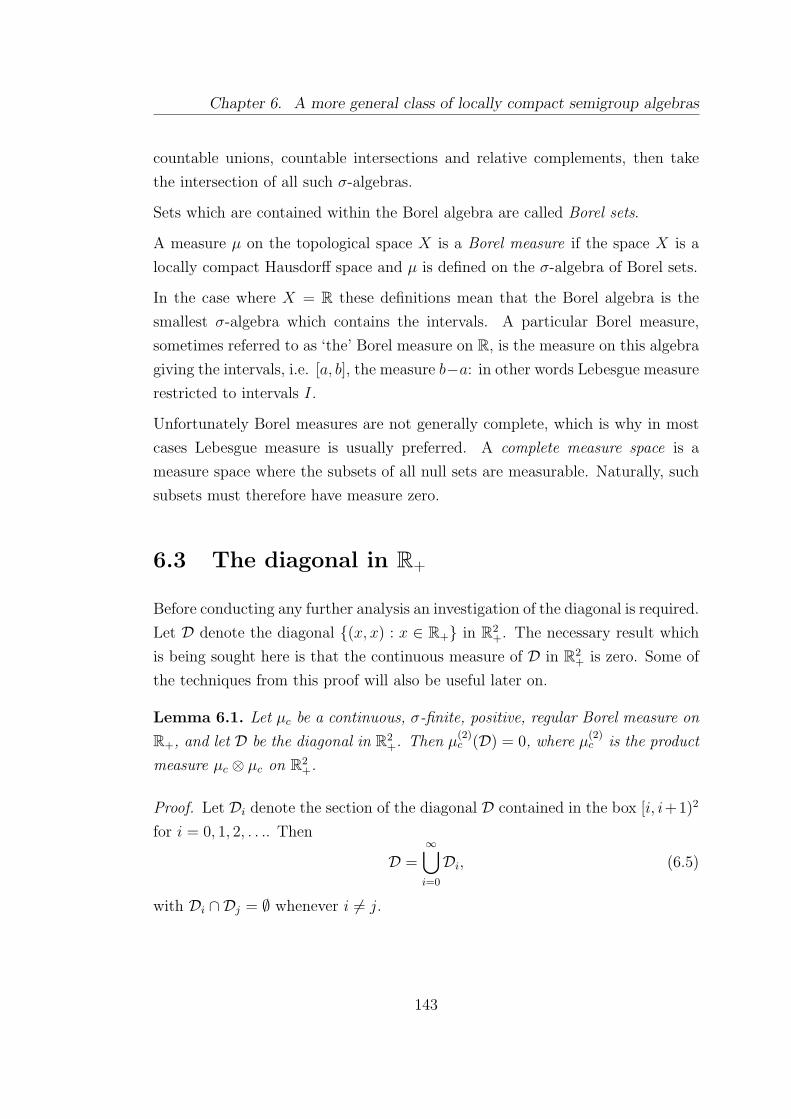
Chapter 6. A more general class of locally compact semigroup algebras
countable unions, countable intersections and relative complements, then take
the intersection of all such σ-algebras.
Sets which are contained within the Borel algebra are called Borel sets.
A measure µ on the topological space X is a Borel measure if the space X is a
locally compact Hausdorff space and µ is defined on the σ-algebra of Borel sets.
In the case where X = R these definitions mean that the Borel algebra is the
smallest σ-algebra which contains the intervals. A particular Borel measure,
sometimes referred to as ‘the’ Borel measure on R, is the measure on this algebra
giving the intervals, i.e. [a, b], the measure b−a: in other words Lebesgue measure
restricted to intervals I.
Unfortunately Borel measures are not generally complete, which is why in most
cases Lebesgue measure is usually preferred. A complete measure space is a
measure space where the subsets of all null sets are measurable. Naturally, such
subsets must therefore have measure zero.
6.3 The diagonal in R+
Before conducting any further analysis an investigation of the diagonal is required.
Let D denote the diagonal {(x, x) : x ∈ R+} in R2+. The necessary result which
is being sought here is that the continuous measure of D in R2+ is zero. Some of
the techniques from this proof will also be useful later on.
Lemma 6.1. Let µc be a continuous, σ-finite, positive, regular Borel measure on
R+, and let D be the diagonal in R2+. Then µ
(2)c (D) = 0, where µ
(2)c is the product
measure µc ⊗ µc on R2+.
Proof. Let Di denote the section of the diagonal D contained in the box [i, i+1)2
for i = 0, 1, 2, . . .. Then
D =∞⋃i=0
Di, (6.5)
with Di ∩ Dj = ∅ whenever i 6= j.
143

Chapter 6. A more general class of locally compact semigroup algebras
So by countable additivity
µ(2)c (D) = µ(2)
c
(∞⋃i=0
Di
)=∞∑i=0
µ(2)c (Di). (6.6)
Without loss of generality consider D0 ⊂ [0, 1)2. The method is to dyadically
split the interval [0, 1) into subintervals of equal measure.
Now we define Ea1···an as
Ea1···an =
[0, α0···0), a1 · · · an = 0 · · · 0,
[αa1···an−0···01, αa1···an), else,(6.7)
with ai = 0 or 1 for i = 1, . . . , n and α1···1 = 1.
Pictorially this is:
[0,1)
E[0,α0)
E0� [α0,1)
E1
-
[0,α00)
E00
� [α00,α01)
E01
-[α01,α10)
E10
� [α10,1)
E11
-
· · ·� · · ·-
· · ·� · · ·-
· · ·� · · ·-
· · ·� · · ·-
Notice that the top level is where n = 0, the second level (containing E0 and E1)
is where n = 1 and so on.
Consider [0, 1), and define
α0 = sup
{t ∈ [0, 1) : µc([0, t)) ≤
1
2µc([0, 1))
}. (6.8)
Then µc([0, αo)) = 12µc([0, 1)). For if t < α0 then µc([0, t)) ≤ 1
2µc([0, 1)) by
definition. Also µc([0, α0− 1n)) ≤ µc([0, α0)) ≤ 1
2µc([0, 1)), again by definition for
all n ∈ N. Finally µc([0, α0 + 1n)) ≥ 1
2µc([0, 1)) for all n ∈ N, else α0 would not
be the supremum.
Thus by continuity from above and below
µc([0, α0)) =1
2µc([0, 1)). (6.9)
144

Chapter 6. A more general class of locally compact semigroup algebras
Then in turn
µc([α0, 1)) =1
2µc([0, 1)) (6.10)
by countable additivity.
Similar arguments hold for every splitting. Thus
µc(Ea1···an0) = µc(Ea1···an1) =1
2µc(Ea1···an), (6.11)
or in other words every child receives exactly half the measure of its parent. The
reason for this construction will become clear later on.
Now make the inductive definitions
Mn =⋃
ai=0 or 1
E2a1···an
, (6.12)
such that
M1 = E20 ∪ E2
1 ,
M2 = E200 ∪ E2
01 ∪ E210 ∪ E2
11,
...
(6.13)
with M0 = E2 = [0, 1)2.
Then D0 ⊆Mn for all n ∈ Z+ and M0 ⊇M1 ⊇M2 ⊇ · · · . In fact
limn→∞
Mn = D0 i.e.∞⋂n=0
Mn = D0. (6.14)
Thus the box [0, 1)2 has been split up into smaller and smaller disjoint boxes
which collectively contain the diagonal.
It is now necessary to prove that µ(2)c (Mn)→ 0 as n→∞.
It follows that
µ(2)c (Mn) =
∑ai=0 or 1
µ(2)c (E2
a1···an) =
∑ai=0 or 1
µ2c(Ea1···an), (6.15)
as Mn =⋃ai=0 or 1E
2a1···an
and these boxes are pairwise disjoint.
145
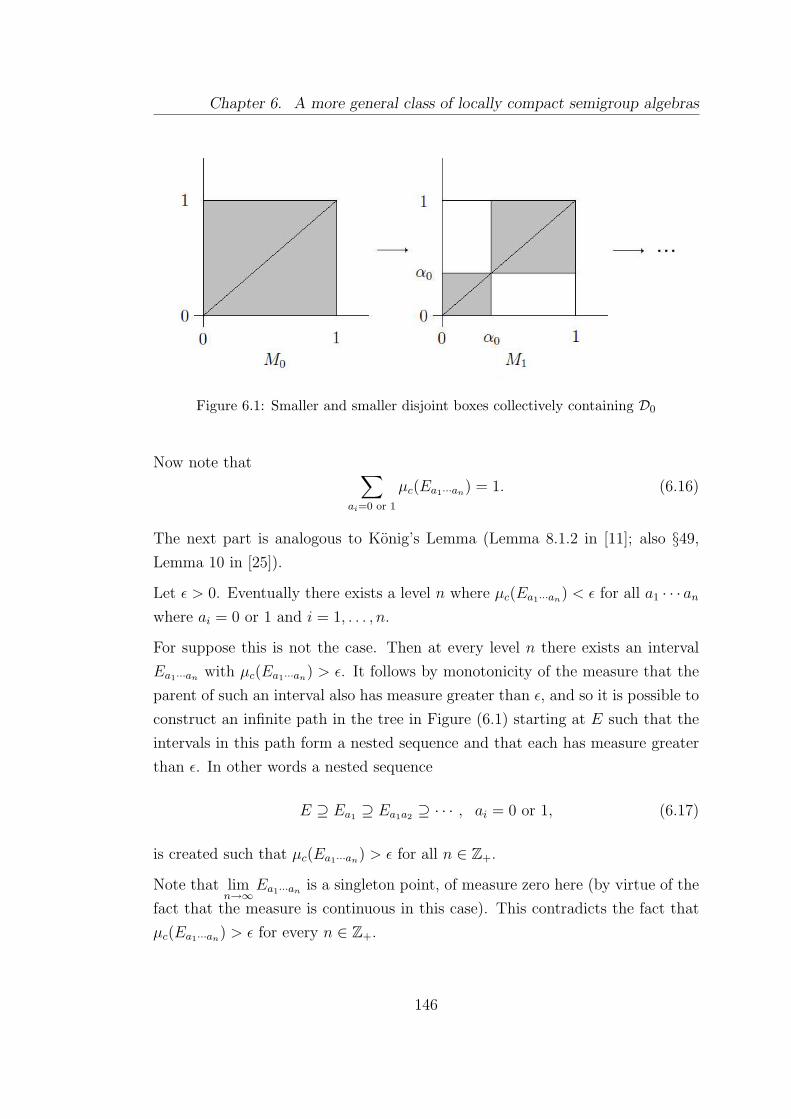
Chapter 6. A more general class of locally compact semigroup algebras
Figure 6.1: Smaller and smaller disjoint boxes collectively containing D0
Now note that ∑ai=0 or 1
µc(Ea1···an) = 1. (6.16)
The next part is analogous to Konig’s Lemma (Lemma 8.1.2 in [11]; also §49,
Lemma 10 in [25]).
Let ε > 0. Eventually there exists a level n where µc(Ea1···an) < ε for all a1 · · · anwhere ai = 0 or 1 and i = 1, . . . , n.
For suppose this is not the case. Then at every level n there exists an interval
Ea1···an with µc(Ea1···an) > ε. It follows by monotonicity of the measure that the
parent of such an interval also has measure greater than ε, and so it is possible to
construct an infinite path in the tree in Figure (6.1) starting at E such that the
intervals in this path form a nested sequence and that each has measure greater
than ε. In other words a nested sequence
E ⊇ Ea1 ⊇ Ea1a2 ⊇ · · · , ai = 0 or 1, (6.17)
is created such that µc(Ea1···an) > ε for all n ∈ Z+.
Note that limn→∞
Ea1···an is a singleton point, of measure zero here (by virtue of the
fact that the measure is continuous in this case). This contradicts the fact that
µc(Ea1···an) > ε for every n ∈ Z+.
146

Chapter 6. A more general class of locally compact semigroup algebras
Hence for large enough n it follows that
0 ≤ µc(Ea1··· n) < ε. (6.18)
Thus, again assuming n is large enough,
µ(2)c (Mn) =
∑ai=0 or 1
µ(2)c (E2
a1···an)
=∑
ai=0 or 1
(µc(Ea1···an))2, (product measure),
<∑
ai=0 or 1
ε · µc(Ea1···an), (by above argument),
= ε ·∑
ai=0 or 1
µc(Ea1···an)
= ε · 1, (by (6.16))
= ε,
(6.19)
and thus
µ(2)c (Mn) < ε for all n > N ∈ N and ε > 0. (6.20)
Hence by definition µ(2)c (Mn)→ 0 as n→∞.
Using this it now follows that
µ(2)c (D0) = µ(2)
c
(∞⋂n=0
Mn
)= lim
n→∞µ(2)c (Mn) = 0 (6.21)
by continuity from above and below, i.e. µ(2)c (D0) = 0.
A similar argument holds for all i ∈ Z+ to obtain the result
µ(2)c (Di) = 0. (6.22)
Hence, finally, we are able to conclude that
µ(2)c (D) =
∞∑i=0
µ(2)c (Di) =
∞∑i=0
0 = 0, (6.23)
147

Chapter 6. A more general class of locally compact semigroup algebras
or in other words
µ(2)c (D) = 0, (6.24)
as required.
6.4 Adjusting the spreading out function
In Chapters 4 and 5 we necessarily created and used the spreading-out functions
εk and γk. Such functions are once again necessary here but they need adjusting
to accommodate the changes in the measure; this will become more apparent as
the proceeding analysis continues.
Consider the division of R+ into intervals of length one, where Ii = [i, i + 1).
As in the previous section divide each of these intervals dyadically so that each
division imparts half of the currently available measure, and let E(i)a1···an denote
the dyadic intervals at the nth level of interval Ii.
Now let fE
(i)a1···an
∈ C, where fE
(i)a1···an
is a function in C defined on the interval
E(i)a1···an .
Definition. The spreading-out function γk : C → C⊗C is defined for fE
(i)a1···an
by
the formula
γk(fE
(i)a1···an
)(x,y)=γk,y(fE
(i)a1···an
)(x)=
fE
(i)0···0
(x)χE
(i−1)1···1
(y)
µc(E(i−1)1···1 )
, a0 · · · an = 0 · · · 0, i ≥ 1,
fE
(i)a1···an
(x)χE
(i)a1···an
(y)
µc(E(i)(a1···an)′)
, else,
(6.25)
where (a1 · · · an)′ = a1 · · · an − 0 · · · 01; in other words (a1 · · · an)′ is the binary
number (a1 · · · an) minus 1.
The spreading-out function then applies to a general f ∈ C by linearity; for given
148
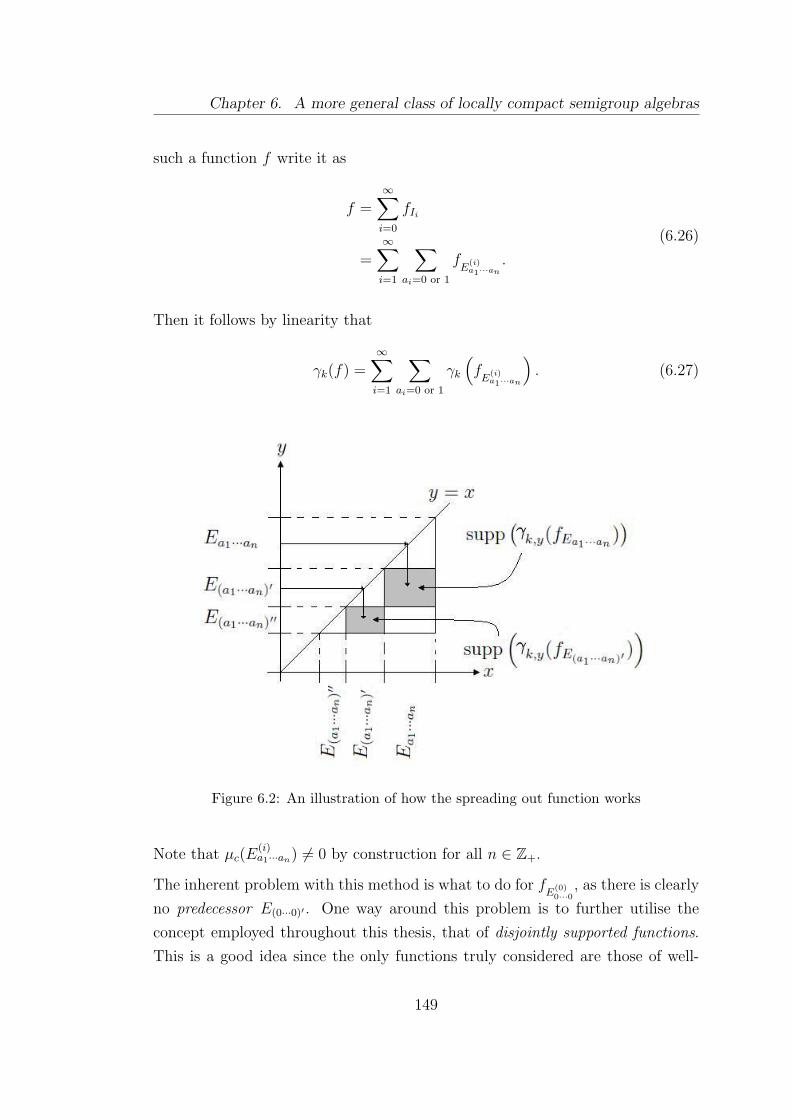
Chapter 6. A more general class of locally compact semigroup algebras
such a function f write it as
f =∞∑i=0
fIi
=∞∑i=1
∑ai=0 or 1
fE
(i)a1···an
.
(6.26)
Then it follows by linearity that
γk(f) =∞∑i=1
∑ai=0 or 1
γk
(fE
(i)a1···an
). (6.27)
Figure 6.2: An illustration of how the spreading out function works
Note that µc(E(i)a1···an) 6= 0 by construction for all n ∈ Z+.
The inherent problem with this method is what to do for fE
(0)0···0
, as there is clearly
no predecessor E(0···0)′ . One way around this problem is to further utilise the
concept employed throughout this thesis, that of disjointly supported functions.
This is a good idea since the only functions truly considered are those of well-
149

Chapter 6. A more general class of locally compact semigroup algebras
separated supports.
Thus given a function f ∈ C assume that χ{(−1,0]} � f , i.e. that there is a
clear separation between the point 0 and the support of f . So when given such
a function f there exists N ∈ N such that for all n ≥ N it follows that E(0)0···0 *
supp(f).
The reason that this is possible is due to the fact that the step/characteristic
function are dense in L1-spaces (Chapter 3, Theorem 3.5). Thus the assumption
that χ{0} � f is representative of this fact.
An alternative is to note that, as in Section 5.1.1, we are only applying the
spreading out function to indicator functions that are not only well-separated
from zero but are also order related to another indicator function which has
support between zero and the support of our function.
6.4.1 The inverse to the spreading out function
As before we will require a left inverse to the spreading-out function γk. Following
the same premise as before we define this function πk : C⊗C→ C as
πk(FJ×J−)(x) =
∫[0,x)
FJ×J−(x, t)dµc(t) +
∫[0,x)
FJ×J−(t, x)dµc(t), (6.28)
where FJ×J− ∈ C⊗C is supported on the domain J × J− where
J = E(i)a1···an
⇒ J− = E(i)(a1···an)′ , a1 · · · an 6= 0 · · · 0,
or J = E(i)0···0 ⇒ J− = E
(i−1)1···1 .
(6.29)
The crucial assumption here is that n is taken large enough to ensure the clear
separation from {0} argument holds as above, making
fE
(0)0···0≡ 0. (6.30)
150

Chapter 6. A more general class of locally compact semigroup algebras
Then it follows for J and J− defined above that
πk(γk(fJ))(x) =
∫ x
0
γk(fJ)(x, t)dt+
∫ x
0
γk(fJ)(t, x)dt
=
∫ x
0
fJ(x)χJ−(t)
µc(J−)dt+
∫ x
0
fJ(t)χJ−(x)
µc(J−)dt
= fJ(x)µc(J−)
µc(J−)+ 0
= fJ(x).
(6.31)
The second term vanishes because we require that x ∈ J in order to avoid the
trivial outcome where everything reduces simply to zero and so the characteristic
function over J− vanishes, while the first term sees the whole of the characteristic
function in t integrated out leaving behind the measure of its domain, namely
µc(J−).
Finally observe that if J = E(0)0···0 then fJ ≡ 0 and it then follows that πk(γk(fJ)) ≡
0, too.
Hence it follows that πk is a left inverse for γk.
6.4.2 The approximate module property
Consider fJ and gK with K being defined similarly to J , which is given above,
such that gK � fJ and fJ , gK are normalised as always. It is now necessary to
see what happens when γk(fJ) and gK are convolved together.
To maintain consistency in notation it is imperative to define, where a ∈ C,
G ∈ C⊗C,
(a ∗G)(x, y) =
∫ x
0
a(t)dt ·G(x, y) + a(x) ·∫ x
0
G(t, y)dt, (6.32)
and
(G ∗ a)(x, y) =
∫ y
0
G(x, t)dt · a(y) +G(x, y) ·∫ y
0
a(t)dt, (6.33)
for then it follows that for G = f ⊗ g
(f ⊗ g) ∗ a = f ⊗ (g ∗ a) & a ∗ (f ⊗ g) = (a ∗ f)⊗ g. (6.34)
151
Chapter 6. A more general class of locally compact semigroup algebras
Using this setup, and noting that n is sufficiently large enough to ensure that the
intervals are well separated and ordered such that K is below J− which is in turn
below J , yields that
(γk(fJ) ∗ gK)(x, y) =
∫ y
0
γk(fJ)(x, t)dt · gK(y) + γk(fJ)(x, y) ·∫ y
0
gK(t)dt
= fJ(x) ·∫ y
0
χJ−(t)
µc(J−)dt · gK(y) + fJ(x) ·
χJ−(y)
µc(J−)·∫ y
0
gK(t)dt.
(6.35)
For this entire expression to be nontrivial it is necessary that y ∈ J−, for if, in
particular, y ∈ K then everything reduces to zero. Then the first term reduces
to zero regardless as the limits of the integral do not reach the domain of χJ−
while the integral in the second term is simply 1 as the limits cover the whole of
the domain of the normalised function gK .
Hence this whole expression reduces simply to
(γk(fJ) ∗ gK)(x, y) = 0 + fJ(x) ·χJ−(y)
µc(J−)· 1 = γk(fJ)(x, y). (6.36)
An almost identical calculation reveals that
(gK ∗ γk(fJ))(x, y) = γk(fJ)(x, y). (6.37)
Consideration of what happens for these calculations when fJ � gk, as in Chapter
5, is possible and follows in a similar way. As these calculations do not appear in
our analysis we will not include them here and leave them for the reader.
6.5 The simplicial cohomology groups
of L1(R+,≤, µc)
It is already known from [3] that HH1(C) ∼= C∗ which, as has already been stated,
is isomorphic to L∞(R+,≤, µc). We now show that for n ≥ 2 we have that
HHn(C) ∼= 0. (6.38)
152
Chapter 6. A more general class of locally compact semigroup algebras
The analysis here follows identically to that in Sections 5.2.2 and 5.2.3.
First we consider the (n + 1)-dimensional tensor product η = f1 ⊗ · · · ⊗ fn ⊗ f0
in⊗n+1
C of normalised functions of disjoint support with the functions fi ∈ C
satisfying some order structure for i = 0, . . . , n in the cyclic context. Because of
cyclicity we are once again able to consider the case when fi � f1 for i 6= 1.
Because of the work done earlier in the current section we are in a position to
define our contracting homotopy of our cyclic chain and cochain complexes here
exactly as found previously, namely that in (5.130) and (5.127) but with C in
place of B, defining snk , sn∗ , δ
n and dn in the same way. We are again able to
approximate γk(f1) by a linear combination of elementary tensor products of
normalised functions of disjoint support,∑∞
i=1 xi ⊗ yi, with fj � xi � yi for all
i = 1, 2, . . ., j 6= 1 and large enough k; this is analogous to the approximation of
γk,y(f1).
We follow the calculations found in Section 5.2.3 through and arrive at the con-
clusion
η = snk,y ◦ dn(η) + dn+1 ◦ sn+1k,y (η) (6.39)
and thus for ϕ ∈ ZCn(B)
ϕ(η) = ϕ(snk,y ◦ dn(η)) + ϕ(dn+1 ◦ sn+1k,y (η)), (6.40)
where the operation of taking limits ensures our disjointedness criteria are met
once more.
We are immediately able to conclude that the second term is trivial as before,
and by duality arguments and a relabeling we therefore see that
ϕ(η) = (δnψ)(η) (6.41)
and hence
HCn(C) ∼= 0 (6.42)
for all n ∈ N.
An appeal to the Connes-Tzygan long exact sequence as in Section 5.2.4 yields
that
HHn(C) ∼= 0 (6.43)
153
Chapter 6. A more general class of locally compact semigroup algebras
for all n ≥ 2.
Considering the first part of the sequence as given in Section 2.2.3 we see that
the sequence
· · · - 0 - HH1(C) - HC0(C) - 0 - · · ·
is exact.
Note that the space HC0(C) is exactly the space of traces on the algebra C which
is isomorphic to C∗; this is a well-known identification. Then we have that
0 = im(0→ HH1(C)) = ker(HH1(C)→ C∗) (6.44)
and so the map from HH1(C) into C∗ is injective, while
im(HH1(C)→ C∗) = ker(C∗ → 0) = C∗ (6.45)
shows that the map is also surjective. Thus we have an isomorphism, showing us
that
HH1(C) ∼= C∗ (6.46)
exactly as before.
6.6 Extending to a general totally ordered, lo-
cally compact semigroup
We now extend our results to the most general case for a continuous, σ-finite,
regular, positive Borel measure µc; changing (R+, ∨) in our algebra to (X, ∨), a
general totally ordered semigroup which is locally compact its order topology, as
defined in Section 2.1. Because there will be no ambiguity, we will drop the ∨
notation.
First we investigate the structure of the semigroup (X,≤, µc). The method is
similar to that found in [2].
Definition. Define the equivalence relation ≈ such that for x, y ∈ X and x ≤ y
we have x ≈ y if µc([x, y)) < ∞. It is straightforward to see that this is indeed
154
Chapter 6. A more general class of locally compact semigroup algebras
an equivalence relation, which we leave to the reader to show.
Definition. A transversal is a set containing exactly one element from each
member of a collection.
We now prove the following necessary result about X.
Lemma 6.2. The equivalence classes of X under the relation ≈ are disjoint and
totally ordered intervals.
Note. In our case, given the nature of later calculations, we are dealing with
countably many equivalence classes here (therefore making the transveral here
possess countably many elements). A problem arises if µc((a, b)) = 0 for a, b ∈ Xsuch that a 6= b. One way to counter such a problem is to insist on the measure
being strictly positive, that is the support of µc is the whole space X; this ensures
that every nonempty open interval in X has strictly positive measure and is hence
infinite. Lebesgue measure is strictly positive.
Proof. Let x ≈ x′ in [x] and y ≈ y′ in [y], where [·] denotes the equivalence class
of ·, such that x � y and therefore x′ � y′.
As x and y are in different equivalence classes it must be that µc([x, y)) = ∞.
We also have that µc([x, x′)) <∞ and µc([y, y
′)) <∞. Thus
∞ = µc([x, y)) ≤ µc([x, x′)) + µc([x
′, y′)) + µc([y, y′)) (6.47)
by the triangle inequality. Since µc([x, x′)) and µc([y, y
′)) are both finite it must
be that µc([x′, y′)) = ∞ and hence x′ and y′ are in different equivalence classes.
Therefore [x] and [y] are disjoint.
To prove that the equivalence classes are totally ordered we use representatives.
For transitivity, if [x] ≤ [y] and [y] ≤ [z] then x ≤ y and y ≤ z for all x ∈ [x], y ∈[y] and z ∈ [z]. As x, y, z ∈ X and X is totally ordered it trivially follows that
x ≤ z for all x ∈ [x] and z ∈ [z], and thus [x] ≤ [z].
Now if [x] ≤ [y] then it must be that x ≤ y for all x ∈ [x], y ∈ [y]. As X is totally
ordered we cannot have y ≤ x for any x ∈ [x], y ∈ [y] and so we cannot have
[y] ≤ [x].
155

Chapter 6. A more general class of locally compact semigroup algebras
The hardest part is proving antisymmetry. Let [x] ≤ [y] and [y] ≤ [x]. Then we
can choose representatives x ∈ [x], y ∈ [y] such that x ≤ y. We are also able to
choose representatives x′ ∈ [x], y′ ∈ [y] such that y′ ≤ x′.
Within the equivalence class [x] one of x ≤ x′ or x′ ≤ x must hold. If x ≤ x′ then
we can conclude that y′ ≤ x′ ≤ x ≤ y, and so by inclusion and non-negativity
of measures µc([x, y)) ≤ µc([y′, y)) < ∞ as y and y′ are in the same equivalence
class.
On the other hand, if x ≤ x′ then either y′ ≤ x or x ≤ y′. If y′ ≤ x then we have
that y′ ≤ x ≤ y, and thus µc([x, y)) ≤ µc([y′, y)) < ∞. If x ≤ y′ then we have
that x ≤ y′ ≤ x′ and hence µc([y′, x′)) ≤ µc([x, x
′)) < ∞ as x and x′ are in the
same equivalence class.
This covers every possibility and in all of the cases we have for x ∈ [x], y ∈ [y]
that µc([x, y)) <∞ and so x ≈ y or [x] = [y] as required.
To see that the equivalence classes are intervals in X we choose a ∈ [a] and define
the function γ : [a]→ R by the formula
γ(x) = µc([a, x)), (6.48)
γ(x′) = µc([x′, a)), (6.49)
for x, x′ ∈ [a] such that x′ ≤ a ≤ x. Then it is not hard to see, given the condition
of strict positivity, that imγ = J , an interval in R such that 0 ∈ J . It follows
that γ is a bijection from [a] onto J and so the two are isomorphic.
The multiplication in our semigroup X is simply an extension of the multipli-
cation in each of the individual semigroups that go into making its sum. Let
[ai], [aj] be equivalence classes in X under ≈ such that i ≤ j, say. If i < j then
ai < aj and [ai] ∩ [aj] = ∅, i.e. the intervals are ordered and disjoint. If on the
other hand i = j then [ai] = [aj].
Then for s ∈ [ai] and t ∈ [aj] we have that
s∨t =
t, i < j,
s∨t, i = j.(6.50)
156

Chapter 6. A more general class of locally compact semigroup algebras
It should be noted at this point that equivalence classes under the relation ≈ in
X are open. For if x ∈ [a] then local compactness implies that there exists a
compact neighbourhood of x. Using this neighbourhood we are able to find an
open interval of finite length I (take the maximum and minimum elements of
the totally ordered neighbourhood) which contains x such that I ∪ [a] = I. So
I ⊆ [a].
As this holds for every point of [a] we are able to write [a] as an arbitrary union
of open intervals, making it open.
It should also be noted that using the same logic and Ic, the complement of
I, instead we can also write [a] as an arbitrary intersection of closed intervals,
making [a] closed as well.
We are now able to see that X can be written as a union of disjoint, totally
ordered intervals;
X =⊔i∈T
[xi], (6.51)
where T is a countable transversal of X/ ≈.
We can therefore consider L1(X,≤, µc) to be equivalent to the `1-direct sum⊕i∈T
L1([ai],≤, µc). (6.52)
The fundamental result of this section is now presented as:
Theorem 6.1. Let [a] be an equivalence class in X under the relation ≈. Then
L1([a], µc) ∼= L1((b, c), λ), (6.53)
where b, c ∈ R ∪ {±∞} and λ is Lebesgue measure.
Note that b, c could be ±∞ or simply finite numbers in R. As we are dealing with
continuous measures it follows that the inclusion or exclusion of the endpoints
b, c is a null point, especially as [a] is both open and closed.
Proof. We have shown that [a] is an interval, say (x, y); this could be unbounded
in either or both directions. Let f ∈ L1([a], µc) ≡ L1((x, y), µc) and fix the
157

Chapter 6. A more general class of locally compact semigroup algebras
point a ∈ [a] = (x, y) ⊆ X. It should be noted that a cannot be an unattain-
able endpoint (although it can be a finite endpoint) due to the definition of the
equivalence relation ≈, i.e. there exist x1, x2 ∈ [a] such that x1 < a < x2.
We now define the transformation τ : (x, y)→ (b, c) by the formula
τ(t) =
−µc(t, a), t ≤ a,
+µc(a, t), a < t.(6.54)
Then we have that τ(a) = 0. Thus 0 ∈ (b, c), where b, c ∈ R ∪ {±∞}. Note that
we have no control over what b and c are.
Now given f(t) = g(t) ∈ L1([a], µc) ≡ L1((x, y), µc) such that
g(t) =
1, t ∈ [x1, x2],
0, else,(6.55)
we define the map g 7→ g such that
g(t) = g(τ(t)) (6.56)
for t ∈ [x1, x2] = supp(g) where x ≤ x1 < x2 ≤ y and g ∈ L1((b, c), λ). For these
step functions, which we have scaled to have value 1 on their supports, this is
clearly injective and onto. Additionally, we have that
‖g‖ =
∫ y
x
|g(t)|dµc = µc((x1, x2)). (6.57)
Also
‖g‖ =
∫ c
b
|g(t)|dt =
∫ τ(x2)
τ(x1)
|g(t)|dt, (6.58)
and since for all t ∈ (τ(x1), τ(x2)) = supp(g) there exists t′ ∈ (x1, x2) = supp(g)
such that τ(t′) = t it follows that g(t) = g(τ(t′)) = g(t′) = 1 here and thus∫ τ(x2)
τ(x1)
|g(t)|dt =
∫ τ(x2)
τ(x1)
dt = τ(x2)− τ(x1). (6.59)
158
Chapter 6. A more general class of locally compact semigroup algebras
Then
τ(x2)− τ(x1) =
µc((a, x2))− µc((a, x1)), a ≤ x1 ≤ x2,
−µc((x2, a)) + µc((x1, a)), x1 ≤ x2 ≤ a,
µc((a, x2)) + µc((x1, a)), x1 ≤ a ≤ x2,
(6.60)
which, by countable additivity of µc, is exactly µc((x1, x2)) as required.
Since this holds for step functions, which are dense in L1 algebras, it follows that
the map g 7→ g is an isometric isomorphism.
Now consider step functions f , g ∈ L1([a], µc). We need to show that our isometric
isomorphism preserves the product structure.
Under the isomorphism f is mapped to f such that f(τ(t)) = f(t) while g is
mapped to g such that g(τ(t)) = g(t) for all t ∈ supp(g). The convolution of
these images is then f ∗ g ∈ L1((b, c), λ). But for all x ∈ (b, c) there exists t ∈ [a]
such that τ(t) = x and so
(f ∗ g)(y) = (f ∗ g)(τ(t)). (6.61)
On the other hand, the product of f and g is a function h in L1([a], µc). Under our
isometric isomorphism this is mapped to the function h such that h(τ(t)) = h(t)
for t ∈ [a]. But
h(t) = (f ∗ g)(t)
=
∫u<t
f(u)dµc(u) · g(t) + f(t) ·∫u<t
g(u)dµc(u).(6.62)
Compare this to
(f ∗ g)(τ(t)) = (f ∗ g)(x) =
∫v<x
f(v)dv · g(x) + f(x) ·∫v<x
g(v)dv. (6.63)
First we can see that as τ is an order-preserving isomorphism it follows that for
the step function with value 1 and supp(f) = (x1, x2)∫v<x
f(v)dv = x− x1. (6.64)
159

Chapter 6. A more general class of locally compact semigroup algebras
But there exist t, t1 such that τ(t1) = x1 and τ(t) = x, and so this becomes
τ(t)− τ(t1) =
µc((a, t))− µc((a, t1)), a ≤ t1 ≤ t,
µc((a, t))− (−µc((t1, a))), t1 ≤ a ≤ t,
−µc((t, a))− (−µc((t1, a))), t1 ≤ t ≤ a,
(6.65)
all of which equate to µc((t1, t)) via countable additivity of µc.
Compare this to ∫u<t
f(u)du = µc((t1, t)). (6.66)
as supp(f) = (x1, x2) implies that supp(f) = (t1, t2) where τ(t2) = x2.
Since for all x there exists t such that τ(t) = x it follows that f(x) = f(τ(t)) =
f(t). As these hold for g as well we have that
h(t) = (f ∗ g)(τ(t)) (6.67)
and since both (f ∗ g)(τ(t)) and h(τ(t)) equal h(t) it follows that h ≡ f ∗ g, i.e.
that f ∗ g is mapped to f ∗ g such that (f ∗ g)(τ(t)) = (f ∗ g)(t); as f is obtained
from f , and similarly for g, this therefore shows that our isomorphism preserves
the product structure of our algebras on step functions.
As the step functions are dense in L1-algebras it follows by density arguments that
this holds for all functions; therefore we have an algebra isometric isomorphism
from L1([a], µc) to L1((b, c), λ) as required.
Essentially this allows us to consider the algebra L1(X,≤, µc) to be a sum of
algebras which are in effect copies (or subalgebras) of L1(R+,≤, λ), L1(R−,≤, λ)
or L1(R,≤, λ).
We are now in a position to make our conclusion. We are able to write
L1(X,≤, µc) ≡`1⊕i∈T
L1((bi, ci), i,≤, λ), (6.68)
where bi, ci ∈ R ∪ {±∞} and i denotes the transversal element indexing the
summand.
160

Chapter 6. A more general class of locally compact semigroup algebras
The product on this algebra is a subtle one, but it must be such that it preserves
the isomorphism of Banach algebras, not just Banach spaces.
Consider the case when X can be decomposed into two intervals; the general case
for n intervals follows from this analysis. Thus we have
L1(X,≤, µc) = L1([xi1 ],≤, µc)⊕ L1([xi2 ],≤, µc). (6.69)
As the equivalence classes of X are ordered we may assume, without loss of
generality, that [xi1 ] < [xi2 ]. Then f, g ∈ L1(X,≤, µc) are such that f = f i1 ⊕ f i2
and g = gi1 ⊕ gi2 , where f i, gi ∈ L1([xi],≤, µc) for i = i1, i2. Then since the
multiplication on L1(X, ,≤, µc) is that of convolution we have that
(f ∗ g)(x) =
∫u<x
f(u)dµc(u) · g(x) + f(x) ·∫u<x
g(u)dµc(u)
=
∫u<x
(f i1 ⊕ f i2)(u)dµc(u) · (gi1 ⊕ gi2)(x)
+ (f i1 ⊕ f i2)(x) ·∫u<x
(gi1 ⊕ gi2)(u)dµc(u)
=
∫u<x
f i1(u)dµc(u) · gi1(x) +
∫u<x
f i1(u)dµc(u) · gi2(x)
+
∫u<x
f i2(u)dµc(u) · gi1(x) +
∫u<x
f i2(u)dµc(u) · gi2(x)
+ f i1(x) ·∫u<x
gi1(u)dµc(u) + f i1(x) ·∫u<x
gi2(u)dµc(u)
+ f i2(x) ·∫u<x
gi1(u)dµc(u) + f i2(x) ·∫u<x
gi2(u)dµc(u).
(6.70)
After collecting terms it is easy to see that
(f ∗ g)(x) = (f i1 ∗ gi1)(x) + (f i1 ∗ gi2)(x) + (f i2 ∗ gi1)(x) + (f i2 ∗ gi2)(x). (6.71)
Hence it must be that the product on⊕
i∈T L1([ai],≤, λ) is
(f ∗ g)(x) = (f i1 ⊕ · · · ⊕ f in) ∗ (gi1 ⊕ · · · ⊕ gin)
=∑t∈T 2
(f t1 ∗ gt2)(x),(6.72)
161
Chapter 6. A more general class of locally compact semigroup algebras
where T = {i1, . . . , in} and t = (t1, t2) here. It is easily seen that our isomorphism
respects this product by linearity.
Remark. The order structure on this algebra is initially decided via transversals.
In decomposing X into its collection of intervals indexed by a transversal, these
intervals are ordered. Thus we can order the transversal elements to preserve this
ordering, i.e. if [xi] < [xj] in X/ ≈ then i < j in T .
Thus if fi ∈ L1([xi],≤, µc) ∼= L1((bi, ci), i,≤, λ) for i = i1, i2 then fi1 � fi2
regardless of the relative positioning of the intervals (bi1 , ci1) and (bi2 , ci2); essen-
tially the transversal is the component used to determine order initially. If the
two functions are indexed by the same transversal element then relative order is
arrived at in the usual way, identical to that used for the case when X = R+.
We are thus able to consider L1(X,≤, µc) as an `1 direct sum of L1 algebras
defined on intervals (bi, ci) for i ∈ T , a transversal set for X/ ≈.
We are now interested in showing the triviality of the cyclic cohomology groups for
this algebra D = L1(X,≤, µc). To do this we will again show that a contracting
homotopy exists here, again exactly as in (5.130) and (5.127) (but with D instead
of B), with snk , sn∗ , δ
n and dn defined as found there, by proving the identity
snk ◦ dn + dn+1 ◦ sn+1k = 1 (6.73)
exactly as in Section 5.2.
Consider the elementary tensor product η = f1⊗ · · · ⊗ fn⊗ f0 ∈⊗n+1
D; by the
density and overlapping arguments prevalent throughout this thesis it is enough
to consider the functions fj for j = 0, . . . , n to have ordered and disjoint supports
inX. It should be noted that, as before, snk is also well-defined for η ∈ CCn(D) too,
but as we are following the method in Section 5.2.3 it is necessary to consider a
general tensor product rather than a cyclic one; for in the analysis in Section 5.2.3
we then, implicitly, make the connection with CCn(D) enabling us to introduce
ϕ ∈ ZCn(D), which is where the cyclicity comes in, and move to the dual and
thus our ultimate conclusion: that HCn(D) is trivial for all n ∈ N.
As X is a disjoint union of its equivalence classes under the relation ≈, we may
162

Chapter 6. A more general class of locally compact semigroup algebras
write each fj as the direct sum⊕
i∈T fij . It then follows by linearity that
(snk ◦dn+dn+1◦sn+1k )(η) =
⊕t∈Tn+1
(snk ◦dn+dn+1◦sn+1k )(f t1j1⊗· · ·⊗f
tnjn⊗f t0j0 ). (6.74)
Calculating this directly would be very computationally intensive as we would
have to consider all of the possible order cases within each interval defined by a
transversal element, of which there are many. Therefore we try to emulate what
we have done in the previous chapter; we will show that each of the arguments
of the summands can be embedded into L1(R+,≤, λ) and so conclude that the
identity holds as before.
Let f, g ∈ D and write X as a disjoint union of its equivalence classes,
X =⊔i∈T
[ai]. (6.75)
Using our map τ from [ai] ≡ (x, y) ⊆ X to (bi, ci) ⊆ R, we define a family of
submaps, τi such that
[ai]k = τ−1i ((bi, ci) ∩ [k, k + 1)) . (6.76)
Then we can see that µc([ai]k) ≤ 1 due to the isometric nature of the map τ ,
from which this family is derived, and
X =⊔
(i,k)∈T×Z
[ai]k, (6.77)
which induces the associated map τ ∗i : L1([ai])→ L1(bi, ci) such that τ ∗i ◦f = f◦τi.
Without loss of generality suppose that f, g ∈ D are supported on⊔
(i,k)∈F
[ai]k,
where F ⊆ T × Z such that |F | < ∞; in other words assume f, g are supported
on finite (or compact) intervals. We obtain the general case by expanding through
density arguments once again.
We then define τF :⊔
(i,k)∈F
[ai]k → R+ with the formula
τF ([ai]k) = [2`(i,k), 2`(i,k) + 1), (6.78)
163
Chapter 6. A more general class of locally compact semigroup algebras
where `(i,k) = | {(i′, k′) : (i′, k′) < (i, k)} |. For instance, the minimum in F (which
exists due to the total ordering of T ×Z), say, (i0, k0), results in the unit interval
section [ai0 ]k0 being mapped to the unit interval [0, 1) in R+, with its immediate
successor in F being mapped to [2, 3) and so on.
The map induced by τF , τ ∗F , is then a map from L1([ai], µc) to L1(R+, µc), the
latter of which is isometrically isomorphic to L1(R+, λ), such that
τ ∗F (f ∗ g) = τ ∗F (f) ∗ τ ∗F (g), (6.79)
by analogy to the isomorphism in Theorem (6.1), meaning that we have success-
fully embedded the element f ∈ L1(⊔
(i,k)∈F [ai]k, µc) into L1(R+, λ).
This means that we may consider f t1j1 ⊗· · ·⊗ ftnjn⊗ f t0j0 as an element of L1(Rn+, λ)
for which we already know that
(snk ◦ dn + dn+1 ◦ sn+1k )(f t1j1 ⊗ · · · ⊗ f
tnjn⊗ f t0j0 ) = 1, (6.80)
and hence it follows that⊕t∈Tn+1
(snk ◦dn+dn+1◦sn+1k )(f t1j1 ⊗· · ·⊗f
tnjn⊗f t0j0 ) =
⊕t∈Tn+1
1⊕i∈T L
1([ai],≤,µc), (6.81)
which is the identity on⊕
i∈T L1([ai],≤, µc) as required.
Remark. We may be worried that applying the s-maps to a function may spread
the support of that function beyond the interval in which it is defined, but as
we only apply these maps to the function with the biggest support in the order
structure on the supports it means that we only ever apply it to functions that are
well-separated from the lower edge of each interval. Therefore there will always
be scope to apply these maps.
Alternatively we could also invoke the separation from zero argument found in
Section 6.4.
From our analysis, identical to that in Section 5.2.3, it then follows that the cyclic
cohomology groups of D = L1(X,≤, µc) are also trivial, that is
HCn(D) ∼= 0, for all n ∈ N. (6.82)
164
Chapter 6. A more general class of locally compact semigroup algebras
The Connes-Tzygan long exact sequence used exactly as before then yields to us
the final result of this thesis:
Theorem 6.2. Let (X,≤) be a totally ordered semigroup which is locally compact
in its order topology and let µc be a continuous, σ-finite, regular, positive Borel
measure. Then we have for n ∈ N,
HHn(L1(X,≤, µc)) ∼=
(L1(X,≤, µc))∗ ∼= L∞(X,≤, µc), for n = 1,
0, else.(6.83)
165

Chapter 7
Conclusions and further work
Throughout this thesis we have seen that calculating the simplicial cohomology
groups for semigroup algebras in the locally compact case is not an easy task,
despite appearances. Even proving the triviality of higher degrees of these groups
can become very involved, technical and subtle, relying on a multitude of tech-
niques and results.
In Chapter 3 we created an alternative method for calculating the first simplicial
cohomology group with coefficients in L1(R+, ∨), reinforcing the result proven by
Blackmore in [3]. This allowed us to move on to investigating higher degrees,
with the second simplicial cohomology group for L1(R+, ∨) being the focus of
Chapter 4. Our method allowed us to show that this group is trivial.
In considering the nth simplicial cohomology group for this algebra our method
became restrictive and so we were forced to make modifications in order to pro-
ceed, namely using the notion of a contracting homotopy. Chapter 5 dealt with
these changes and then proved the results of Chapter 4 in order to demonstrate
that these modifications do indeed work. The remainder of Chapter 5 took this
modified method and showed that the nth simplicial cohomology group with co-
efficients in L1(R+, ∨) was trivial for n ≥ 2.
We were able to take these methods further in Chapter 6, analysing initially the
case where the underlying semigroup for our algebra is (R+,≤, µc), where µc is
a more general continuous Borel measure than the Lebesgue measure we had
before, and finally the most general case where (R+, ∨) is replaced by a more
166

Chapter 7. Conclusions and further work
general totally ordered, locally compact semigroup (X,≤, ∨); in both cases we
were able to show that the same results apply as those for the algebra L1(R+, ∨).
Despite what we were able to do there are still a number of questions that could
be the source of some further work on this subject. Some possible avenues of
future research are given here.
Question. What would be the effect of changing the underlying total order to a
partial order? For instance one could consider the algebra L1(R2+, ∨) and attempt
to ascertain if this algebra has trivial higher order simplicial cohomology also.
This question has already been answered in some cases by Gourdeau, Lykova
and White in [14] who investigated the higher dimensional simplicial cohomology
groups of L1(Rk+,+).
We might also consider what changes would be wrought to our results if we change
the binary operation within the semigroup, but there appear to be no other
natural operations left to consider; the min operation is intimately connected to
max, which we have considered here, and × to +, which has been considered
elsewhere.
Question. What are the corresponding results for the more general algebras
Lp(X,≤, µc) when 1 < p <∞?
This question has been partially answered by Blackmore in [3] where he looked
at the first simplicial cohomology group of Lp([0, 1],m) where 1 ≤ p <∞ and m
is Lebesgue measure.
Question. Would it be possible to change the continuous, σ-finite, positive,
regular Borel measure on X to a more general Radon measure?
Question. Could we generate Kunneth formulae for our work, for example to
cover the algebras L1(R2+, ∨) and `1(Z2
+, ∨)?
Note that for the algebra `1(Z2+, ∨) the underlying semigroup is a unital semilattice
(via pointwise operations) and so has already been covered by Choi in his paper
[8].
The final point of consideration is to look at what happens if we have a general
measure, not just a continuous measure. Blackmore in [3] states that a σ-finite,
positive, regular Borel measure on X, µ, can be uniquely decomposed into its
167

Chapter 7. Conclusions and further work
discrete and continuous parts, µ = µd + µc. Based on the result from his paper
and from the work we have conducted in Chapter 6 it appears that we are able
to apply the same logic and hence make the following observation:
Conjecture. Let (X,≤, µ) be a totally ordered semigroup which is locally compact
in its order topology, and let µ be a σ-finite, positive, regular Borel measure on
X with discrete part µd and continuous part µc. Then for n ∈ N we have that
HHn(L1(X,≤, µ)) ∼= HHn(L1(X,≤, µd))⊕HHn(L1(X,≤, µc)). (7.1)
We would then be able to consider the discrete and continuous parts separately,
into which a lot of work has gone already. That concludes this thesis.
168

Bibliography
[1] W. G. Bade, P. C. Curtis, and H. G. Dales, Amenability and weak
amenability for Beurling and Lipschitz algebras, Proc. London Math. Soc.
(3), 55 (1987), pp. 359–377.
[2] J. W. Baker, J. S. Pym, and H. L. Vasudeva, Totally ordered measure
spaces and their Lp algebras, Mathematika, (1982).
[3] T. D. Blackmore, Derivations from totally ordered semigroup algebras
into their duals, Canad. Math. Bull., 40(2) (1997), pp. 133–142.
[4] , Weak amenability of discrete semigroup algebras, Semigroup Forum,
55 (1997), pp. 196–205.
[5] F. F. Bonsall and J. Duncan, Complete Normed Algebras, Ergebnisse
der Mathematik und ihrer Grenzgebiete, Band 80, Springer-Verlag, Berlin,
1973.
[6] J. Brodzki and Z. A. Lykova, Excision in cyclic type homology of Frechet
algebras, Bulletin of the London Math. Soc., 33 (2001), pp. 283–291.
[7] M. Capinski and E. Kopp, Measure, integral and probability, Springer
undergraduate mathematics series, Springer, London, 2004.
[8] Y. Choi, Simplicial homology and Hochschild cohomology of Banach semi-
lattice algebras, Glasgow Mathematical Journal, 48 (2006), pp. 231–245.
[9] , Hochschild homology and cohomology of `1(Zk+), The Quarterly Journal
of Mathematics, 61 (2010), pp. 1–28.
[10] Y. Choi, F. Gourdeau, and M. C. White, Simplicial cohomology of
band semigroup alegras, Preprint, arXiv:1004.2301v1 (2010).
169

Bibliography
[11] R. Diestel, Graph Theory, vol. 173 of Graduate Texts in Mathematics,
Springer, Berlin, 2005.
[12] J. B. Fraleigh, A first course in abstract algebra, Addison-Wesley Pub-
lishing Company, 1980.
[13] F. Gourdeau, B. E. Johnson, and M. C. White, The cyclic and
simplicial cohomology of `1(N), Transactions of the American Mathematical
Society, 357 (2005), pp. 5097–5113.
[14] F. Gourdeau, Z. A. Lykova, and M. C. White, The simplicial coho-
mology of L1(Rk+), 363 (2004), pp. 95–109.
[15] , The simplicial cohomology of `1(Zk+) and a Kunneth formula, Studia
Mathematica, 166 (2005), pp. 29–54.
[16] F. Gourdeau, A. Pourabbas, and M. C. White, Simplicial cohomol-
ogy of some semigroup algebras, Canadian Mathematical Bulletin. Bulletin
Canadien de Mathematiques, 50 (2007), pp. 56–70.
[17] F. Gourdeau and M. C. White, Vanishing of the third simplicial coho-
mology group of `1(Z+), Transactions of the American Mathematical Society,
353 (2001), pp. 2003–2017 (electronic).
[18] , The cyclic and simplicial cohomology of the bicyclic semigroup algebra,
to appear in Quarterly Journal of Mathematics, (2010).
[19] A. Hatcher, Algebraic Topology, Cambridge University Press, Cambridge,
2002.
[20] A. Y. Helemskiı, The homology of Banach and topological algebras, Kluwer
Academic Publishers, 1986.
[21] , Banach cyclic (co)homology and the Connes-Tzygan exact sequence, J.
London Math. Soc. (2), 46 (1992), pp. 449–462.
[22] P. J. Hilton and U. Stammbach, A Course in Homological Algebra,
Springer-Verlag, New York, 1997.
170

Bibliography
[23] B. E. Johnson, Cohomology in Banach algebras, Memoirs of the American
Mathematical Society, 127 (1972).
[24] , Derivations from L1(G) into L1(G) and L∞(G), Harmonic analysis
(Luxembourg, 1987), 1359 (1988), pp. 191–198.
[25] S. C. Kleene, Mathematical Logic, John Wiley & Sons, inc., New York,
1967.
[26] J. R. Munkres, Topology, Pearson Education International, 2000.
[27] W. Rudin, Real and complex analysis, 1987.
[28] R. A. Ryan, Introduction to tensor products of Banach spaces, Springer
monographs in mathematics, Springer, London, 2002.
[29] K. Saxe, Beginning functional analysis, Springer, New York, 2002.
[30] C. A. Weibel, An introduction to homological algebra, Cambridge Univer-
sity Press, 1994.
[31] A. J. Weir, General integration and measure, Cambridge University Press,
1974.
171


![félcsoport (semigroup) = ({s},{ * : s s s [infix]}. semigroup is a type specification =](https://img.dokumen.tips/doc/110x75/568146e2550346895db41a6d/felcsoport-semigroup-s-s-s-s-infix-semigroup-is-a-type.jpg)

