Simple Poverty Scorecard® Poverty-Assessment Tool Mali

Mark Schreiner

July 16, 2008

Ce document en français est disponible sur SimplePovertyScorecard.com. This document in English is at SimplePovertyScorecard.com.

Abstract The Simple Poverty Scorecard-brand poverty-assessment tool uses ten low-cost indicators from Mali’s 2001 Poverty Evalution Survey to estimate the likelihood that a household has consumption below a given poverty line. Field workers can collect responses in about ten minutes. The scorecard’s accuracy is reported for a range of poverty lines. The scorecard is a practical way for pro-poor programs in Mali to measure poverty rates, to track changes in poverty rates over time, and to segment clients for targeted services.

Version note This paper includes 1993 PPP poverty lines. A later version—released 30 January 2010—includes 2005 PPP poverty lines. Otherwise, both papers are identical. In particular, the scoreard itself remains the same.

Acknowledgements The paper was funded by Trickle Up and FIDES. Data come from Mali’s Direction Nationale de la Statistique et de l’Information. Thanks go to Malika Anand, Jeffrey Ashe, Gabrielle Athmer, Marième Daff, Dunni Goodman, Judith Larrivière, Nanci Lee, Susannah Hopkins Leisher, Jan Maes, Bamadio Modibo, Vimala Palaniswamy, Don Sillers, Sidi Takiou, Thierry van Bastelaer, and Koenraad Verhagen. “Simple Poverty Scorecard” is a Registered Trademark of Microfinance Risk Management, L.L.C. for its brand of poverty-assessment tools. Copyright © 2017 Microfinance Risk Management.

Author Mark Schreiner directs Microfinance Risk Management, L.L.C. He is also a Senior Scholar at the Center for Social Development at Washington University in Saint Louis.

1

Simple Poverty Scorecard® Poverty-Assessment Tool Interview ID: Name Identifier

Interview date: Participant: Country: MLI Field agent:

Scorecard: 001 Service point: Sampling wgt.: Number of household members:

Indicator Value Points Score A. Five or more 0 B. Four 10 C. Three 13 D. Two 15 E. One 17

1. How many household members are 11 years old or younger?

F. None 25

A. Three or more 0 B. Two 7

2. How many members of the household usually work as their main occupation in agriculture, animal husbandry, fishing, or forestry? C. One or none 14

A. Tile or thatch 0 3. What is the main construction material of the roof of the residence? B. Mud, corrugated metal sheets,

concrete, or other 12

A. Partly cement or others 0 4. What is the main construction material of the walls of the residence? B. Cement 7

A. Surface water, non-modern well, drilled well, or others

0

B. Modern well 3 C. Public pump 6

5. What is the household’s main source of drinking water?

D. Faucet tap 11

A. Others 0 6. What toilet arrangements does the household have?

B. Latrine (private or shared with other households) or flush toilet (private inside, private outside, or shared with other households)

7

A. No 0 7. Does the household own any television sets? B. Yes 6

A. No 0 8. Does the household own any radios? B. Yes 7

A. No 0 9. Does the household own any irons? B. Yes 5

A. No 0 10. Does the household own any motorbikes? B. Yes 6

SimplePovertyScorecard.com Score:

Simple Poverty Scorecard® Poverty-Assessment ToolMali

1. Introduction

Pro-poor programs in Mali can use the Simple Poverty Scorecard poverty-

assessment tool to monitor groups’ poverty rates at a point in time, track changes in

groups’ poverty rates between two points in time, and target services to households.

The direct approach to poverty measurement via expenditure surveys is difficult

and costly, asking households about a lengthy list of consumption items (“Did you serve

breakfast today? If so, for whom? What ingredients did you use? If rice was an

ingredient, how much rice did you use? Did you buy the rice, grow it yourself, or trade

for it? If you bought it, how many units did you buy, how much did you pay per unit,

and how often do you buy it? Now then, was oats an ingredient? . . .”).

In contrast, the indirect approach via poverty scoring is simple, quick, and

inexpensive. It uses 10 verifiable indicators (such as “What is the main construction

material of the floor of the residence?” or “Does the household own any television sets?”)

to get a score that is highly correlated with poverty status as measured by the

exhaustive expenditure survey.

The scorecard here differs from “proxy means tests” (Coady, Grosh, and

Hoddinott, 2002) in that it is tailored to the capabilities and purposes not of national

governments but rather of local, pro-poor organizations. The feasible poverty-

1

measurement options for these organizations are typically subjective and relative (such

as participatory wealth ranking by skilled field workers) or blunt (such as rules based

on land-ownership or housing quality). Results from these approaches are not

comparable across organizations nor across countries, they may be costly, and their

accuracy is unknown.

If an organization wants to know what share of its participants are below a given

poverty line (say, $1/day for the Millenium Development Goals, or the poorest half

below the national poverty line as required of USAID microenterprise partners), or if it

wants to measure movement across a poverty line (for example, to report to the

Microcredit Summit Campaign), then it needs an expenditure-based, objective tool with

known accuracy. While expenditure surveys are costly even for governments, even

small, local organizations can implement an inexpensive scorecard that can serve for

monitoring, management, and targeting.

The statistical approach here aims to be understood by non-specialists. After all,

if managers are to adopt poverty scoring on their own and apply it to inform their

decisions, they must first trust that it works. Transparency and simplicity build trust.

Getting “buy-in” matters; proxy means tests and regressions on the “determinants of

poverty” have been around for three decades, but they are rarely used to inform

decisions, not because they do not work, but because they are presented (when they are

presented at all) as tables of regression coefficients incomprehensible to lay people (with

cryptic indicator names such as “HHSIZE_2”, negative values, many decimal places, and

2

standard errors). Thanks to the predictive-modeling phenomenon known as the “flat

max”, the scorecard can be almost as accurate as a complex tool.

The technical approach here is also innovative in how it associates scores with

poverty likelihoods, in the extent of its accuracy tests, and in how it derives sample-size

formulas. Although these techniques are simple and/or standard, they have rarely or

never been applied to proxy means tests.

The scorecard (Figure 1) is based on data from the 2001 Enquête Malienne sur

L’Evaluation de la Pauvreté (EMEP, Mali Poverty Evaluation Survey) conducted by

Mali’s Direction Nationale de la Statistique et de l’Information (DNSI). Indicators are

selected to be:

Inexpensive to collect, easy to answer quickly, and simple to verify Strongly correlated with poverty Liable to change over time as poverty status changes

All points in the scorecard are non-negative integers, and total scores range from

0 (most likely below a poverty line) to 100 (least likely below a poverty line). Non-

specialists can collect data and tally scores on paper in the field in less than 5 minutes.

Poverty scoring can be used to estimate three basic quantities. First, it can

estimate a household’s “poverty likelihood”, that is, the probability that the household

has per-capita expenditure below a given poverty line.

Second, poverty scoring can estimate the poverty rate of a group of households

at a point in time. This is simply the average poverty likelihood among the households

in the group.

3

Third, poverty scoring can estimate changes in the poverty rate for a group of

households between two points in time. This estimate is simply the change in the

average poverty likelihood of the households in the group over time.

Poverty scoring can also be used for targeting. To help managers choose a

targeting cut-off, this paper reports the share of Mali’s households who are below a

given poverty line and who are also at or below a given score cut-off.

This paper presents a single scorecard (Figure 1) whose indicators and points

were derived using the national poverty line and a sub-sample of Mali’s EMEP. Scores

from this scorecard are calibrated to poverty likelihoods for six poverty lines.

Scorecard accuracy is tested on a different sub-sample of the EMEP than that

used in scorecard construction. While all three scoring estimators are unbiased (that is,

they match the true value on average in repeated samples from the 2001 population),

they are—like all predictive models—biased to some extent when applied to a different

population.

Thus, while the indirect scoring approach is less costly than the direct survey

approach, it is also biased. (The survey approach is unbiased by assumption.) There is

bias because scoring must assume that the future relationship between indicators and

poverty will be the same as in the data used to build the scorecard. Of course, this

assumption—ubiquitous and inevitable in predictive modelling—holds only partly.

The difference between scorecard estimates of groups’ poverty rates and the true

rates ranges from –0.7 percentage points for the $2/day line to 5.0 percentage points for

4

the $3/day line, with an average absolute difference across all six lines of 2.7 percentage

points. These differences are due to sampling variation—not bias—because their

average would be zero if the EMEP were to be repeatedly redrawn and divided into

sub-samples before repeating the entire scorecard-building process.

For sample sizes of n = 16,384, the 90-percent confidence intervals for these

estimated differences are less than +/–1.0 percentage points. For n = 1,024, the 90-

percent intervals are less than +/–4.0 percentage points.

Section 2 below describes data and poverty lines. Section 3 compares the new

scorecard to an existing poverty-assessment tool for Mali. Sections 4 and 5 describe

scorecard construction and offer practical guidelines for use. Sections 6 and 7 detail the

estimation of households’ poverty likelihoods and of groups’ poverty rates at a point in

time. Section 8 discusses estimating changes in poverty rates between two points in

time. Section 9 covers targeting. The final section is a summary.

5

2. Data and poverty lines

This section discusses the data used to construct and test the scorecard. It also

presents the poverty lines to which scores are calibrated.

The scorecard is based on Mali’s 2001 EMEP. DNSI (2004) reports that the

EMEP covers 7,373 households, but the database provided by the DNSI for this paper

includes only 4,933 households. Still, the sum of household weights (themselves

weighted by household size) match Mali’s 10.2 million population in DNSI (2004).

Thus, the missing households appear to have been removed deliberately (albeit without

documentation), with remaining households reweighted to maintain representativeness.

Here, EMEP households are randomly divided into three samples (Figure 2):1

Construction for selecting indicators and points Calibration for associating scores with poverty likelihoods Validation for testing accuracy on data not used in construction or calibration Mali has two official poverty lines (DNSI, 2004). The food line is based on the

expenditure—derived from the 2001 EMEP—required to obtain 2,450 calories

1 The average household in the EMEP represents about 220 households. Before random assignment to sub-samples, households representing more than 500 households are replicated—and their weights evenly divided among their replicates—so that each replicate represents less than 500 households. Of course, the newly replicated households together represent the same number of households as the original heavily weighted household. This replication helps spread heavily weighted households across the construction, calibration, and validation sub-samples, which in turn reduces the influence of any single heavily weighted household on scorecard construction or testing. This does not affect the unbiasedness of scoring estimators in repeated samples, but it does increase precision and thus decreases the average difference between estimates and true values in any given sample (such as the validation sample). It also helps prevent bootstrap estimates from breaking down (see Singh, 1998).

6

(Fcfa271/person/day). The national line is the actual total expenditure (on food and

non-food) by people in the EMEP who consume about 2,450 calories per day

(Fcfa395/person/day).

The national line and the food line are not adjusted for household economies of

scale nor for differences in cost-of-living by urban/rural or region (DNSI, 2004). Indeed,

there are no sub-national price indices for Mali.

Because local pro-poor organizations may want to use different poverty lines, this

paper calibrates scores from its single scorecard (constructed using the national line) to

poverty likelihoods for six lines (figures in parentheses are per-capita daily poverty lines

and household-level poverty rates from Figure 2):

National line (Fcfa395, 57.3 percent) Food line (Fcfa271, 38.0 percent) USAID “extreme” line (Fcfa228, 28.6 percent) $1/day (Fcfa215, 25.4 percent) $2/day (Fcfa431, 61.7 percent) $3/day (Fcfa646, 80.1 percent)

The USAID “extreme” line (U.S. Congress, 2002) is the median expenditure of

households below the national line.

The $1/day line is derived from the following data:

1993 purchase-power parity exchange rate: Fcfa124.89 per $1 1993 CPI (average): 65.87 2001 CPI (average): 105.19 The $1/day line is then 124.89 x (105.19 65.87) x 1.08 = Fcfa215.40 (Sillers,

2006). The $2/day and $3/day lines are multiples of the $1/day line.

7

Poverty rates may be at the person-level or the household-level. The person-level

rate is the share of people in a given group who live in households whose per-capita

expenditure (that is, total household expenditure divided by the number of household

members) is below a given poverty line. The person-level rates in Figure 2 for the

national line and the food line match those in DNSI (2004).

The household-level poverty rate is the share of households in a given group

whose per-capita expenditure is below a given poverty line.

Whereas governments report person-level poverty rates, local pro-poor

development organizations typically report household-level poverty rates. This is

because local organizations want to know the poverty rate of their clients, not the

poverty rate of all people who live in households with their clients.

Given household-level poverty likelihoods, the person-level poverty rate for all

people in a group of households is simply the average of the household-level poverty

likelihoods, weighted by the number of people in each household. Larger households are

more likely to be poor, so the person-level rate exceeds the household-level rate.

8

3. An existing poverty-assessment tool for Mali

Morris et al. (1999) use 1997 data on 275 households in Mali’s rural Lacustre

region to test an approach to poverty assessment that measures “socioeconomic

position” inexpensively so that it can be included in health surveys and epidemiological

studies.

Their indicators are 18 agricultural implements owned by men, 16 kitchen items

owned by women, and about 14 non-gendered consumer durables such as bicycles,

lamps, and chairs. Each indicator’s value is defined as the number of the item that the

household owns. Each indicator’s points are defined as the reciprocal of the share of

households that own the item, so rarer items get more points. (For example, if one-third

of households own gas lamps, then each gas lamp owned gets 1 ÷ (1 ÷ 3) = 3 points.)

The index value is the logarithm of the sum of each indicator multiplied by its points.

Socioeconomic status is defined as the logarithm of the total value of household

assets. Morris et al. then measure accuracy as the correlation coefficient between the

score and socioeconomic status.

The new scorecard here differs from Morris et al. in several ways. First, it has a

directly practical purpose: to help local, pro-poor programs in Mali improve their

service quality and outreach to the poor. In contrast, Morris et al. have purely

methodological aims; indeed, they do not report their tool’s indicators or points.

Second, the new scorecard here is based on a nationally representative database

that is newer and larger.

9

Third, the new scorecard defines socioeconomic status as whether per-capita

household expenditure is below a given poverty line. This is more commonly used in

practice than the logarithm of the value of household assets.

Fourth, the new scorecard produces poverty likelihoods that have absolute units

(index values from Morris et al. have relative units). Furthermore, poverty likelihoods

can be used not only as controls in epidemiological regressions but also for targeting

and for estimating groups’ poverty rates and their changes over time.

Fifth, the new scorecard is tested on data that is not used in its construction. In

contrast, Morris et al. build and test their tool with the same data, leading to

overstated accuracy. Beyond correlation coefficients, this paper reports differences

between estimates and true values, precision, and sample-size formulas.

Sixth, the new scorecard is less costly than Morris et al. (10 indicators versus

about 40) and simpler for non-specialists to understand (no reciprocals or logarithms).

10

4. Scorecard construction

About 100 potential indicators are initially prepared in the areas of:

Family composition (such as female headship and number of children) Education (such as school attendance by children and highest grade completed) Employment (such as sector and salaried status) Housing (such as tenancy status and type of construction) Ownership of durable goods (such as televisions, refrigerators, and automobiles)

Indicators are first screened with the entropy-based “uncertainty coefficient”

(Goodman and Kruskal, 1979) that measures how well an indicator predicts poverty on

its own. Figure 3 lists the best indicators, ranked by uncertainty coefficient. Responses

are ordered starting with those most strongly associated with poverty.

Many indicators in Figure 3 are similar to each other in terms of their

association with poverty. For example, few houses with dirt floors have cement walls or

tile roofs. If a scorecard includes roof and walls, then data on the floor adds little

information about poverty. Thus, many indicators strongly associated with poverty are

not in the scorecard, as they are similar to other indicators that are included.

The scorecard also aims to measure changes in poverty through time. Thus,

some powerful indicators (such as the highest grade completed by a household member)

that are relatively insensitive to changes in poverty are omitted in favor of less-powerful

indicators (such as ownership of radios or irons) that are more sensitive.

The scorecard itself is built using Logit regression on the construction sub-sample

(Figure 2). Indicator selection uses both judgment and statistics (forward stepwise

based on “c”). The first step is to build one scorecard for each candidate indicator,

11

using Logit to derive points. Each scorecard’s accuracy is taken as “c”, a measure of the

ability to rank by poverty status (SAS Institute Inc., 2004).

One of these one-indicator scorecards is then selected based on several factors

(Schreiner et al., 2004; Zeller, 2004), including improvement in accuracy, likelihood of

acceptance by users (determined by simplicity, cost of collection, and “face validity” in

terms of experience, theory, and common sense), sensitivity to changes in poverty

status, variety among indicators, and verifiability.

A series of two-indicator scorecards are then built, each based on the one-

indicator scorecard selected from the first step, with a second candidate indicator

added. The best two-indicator scorecard is then selected, again based on “c” and

judgment. These steps are repeated until the scorecard has 10 indicators.

The final step is to transform the Logit coefficients into non-negative integers

such that total scores range from 0 (most likely below a poverty line) to 100 (least

likely below a poverty line).

This algorithm is the Logit analogue to the familiar R2-based stepwise with least-

squares regression. It differs from naïve stepwise in that the criteria for selecting

indicators include not only statistical accuracy but also judgment and non-statistical

factors. The use of non-statistical criteria can improve robustness through time and,

more important, helps ensure that indicators are simple and make sense to users.

The single scorecard here applies to all of Mali. Evidence from India and Mexico

(Schreiner, 2006a and 2005a), Sri Lanka (Narayan and Yoshida, 2005), and Jamaica

12

(Grosh and Baker, 1995) suggests that segmenting scorecards by rural/urban does not

improve accuracy much.

13

5. Practical guidelines for scorecard use

The main challenge of scorecard design is not to squeeze out the last drops of

accuracy but rather to improve the chances that scoring is actually used (Schreiner,

2005b). When scoring projects fail, the reason is not usually technical inaccuracy but

rather the failure of an organization to decide to do what is needed to integrate scoring

in its processes and to learn to use it properly (Schreiner, 2002). After all, most

reasonable scorecards predict tolerably well, thanks to the empirical phenomenon known

as the “flat max” (Hand, 2006; Baesens et al., 2003; Lovie and Lovie, 1986; Kolesar and

Showers, 1985; Stillwell, Hutton, and Edwards, 1983; Dawes, 1979; Wainer, 1976; Myers

and Forgy, 1963). The bottleneck is less technical and more human, not statistics but

organizational change management. Accuracy is easier to achieve than adoption.

The scorecard here is designed to encourage understanding and trust so that

users will adopt it and use it properly. Of course, accuracy matters, but it is balanced

against simplicity, ease-of-use, and “face validity”. Programs are more likely to collect

data, compute scores, and pay attention to the results if, in their view, scoring does not

make a lot of “extra” work and if the whole process generally seems to make sense.

To this end, the scorecard here fits on one page (Figure 1). The construction

process, indicators, and points are simple and transparent. “Extra” work is minimized;

non-specialists can compute scores by hand in the field because the scorecard has:

Only 10 indicators Only categorical indicators Simple weights (non-negative integers, with no arithmetic beyond addition)

14

A field worker using the paper scorecard would:

Record participant identifiers Read each question from the scorecard Circle the response and its points Write the points in the far-right column Add up the points to get the total score Implement targeting policy (if any) Deliver the paper scorecard to a central office for filing or data entry Of course, field workers must be trained. Quality results depend on quality

inputs. If organizations or field workers gather their own data and have an incentive to

exaggerate poverty rates (for example, if they are rewarded for higher poverty rates),

then it is wise to do on-going quality control via data review and random audits (Matul

and Kline, 2003).2 IRIS Center (2007a) and Toohig (2007) are useful nuts-and-bolts

guides for budgeting, training field workers and supervisors, logistics, sampling,

interviewing, piloting, recording data, and quality control.

In terms of sampling design, an organization must make choices about:

Who will do the scoring How scores will be recorded What participants will be scored How many participants will be scored How frequently participants will be scored Whether scoring will be applied at more than one point in time Whether the same participants will be scored at more than one point in time The non-specialists who apply the scorecard with participants in the field can be:

Employees of the organization 2 If an organization does not want field workers to know the points associated with indicators, then they can use the version of Figure 1 without points and apply the points later in a spreadsheet or database at the central office.

15

Third-party contractors Responses, scores, and poverty likelihoods can be recorded:

On paper in the field and then filed at an office On paper in the field and then keyed into a database or spreadsheet at an office In portable electronic devices in the field and then downloaded to a database The subjects to be scored can be:

All participants (or all new participants) A representative sample of all participants (or of all new participants) All participants (or all new participants) in a representative sample of branches A representative sample of all participants (or of all new participants) in a

representative sample of branches If not determined by other factors, the number of participants to be scored can

be derived from sample-size formulas (presented later) for a desired level of confidence

and a desired confidence interval.

Frequency of application can be:

At in-take only (precluding measuring change in poverty rates) As a once-off project for current participants (precluding measuring change) Once a year or at some other fixed interval (allowing measuring change) Each time a field worker visits a participant at home (allowing measuring change) When the scorecard is applied more than once so as to measure change in

poverty rates, it can be applied:

With two different representative samples With a single sample, scored twice An example set of choices were made by BRAC and ASA, two microlenders in

Bangladesh (each with 7 million participants) who are applying the Simple Poverty

Scorecard tool for Bangladesh (Schreiner, 2006). Their design is that loan officers in a

16

random sample of branches score all participants each time they visit a homestead as

part of their standard due diligence prior to loan disbursement (about once a year).

Responses are recorded on paper in the field before being sent to a central office to be

entered into a database. ASA’s and BRAC’s sampling plans cover 50,000–100,000

participants each.

17

6. Estimates of household poverty likelihoods

The sum of scorecard points for a household is called the score. For Mali, scores

range from 0 (most likely below a poverty line) to 100 (least likely below a poverty

line). While higher scores indicate less likelihood of being below a poverty line, the

scores themselves have only relative units. For example, doubling the score does not

double the likelihood of being above a poverty line.

To get absolute units, scores must be converted to poverty likelihoods, that is,

probabilities of being below a poverty line. This is done via simple look-up tables. For

the example of the national line, scores of 5–9 have a poverty likelihood of 86.9 percent,

and scores of 50–54 have a poverty likelihood of 47.4 percent (Figure 4).

The poverty likelihood associated with a score varies by poverty line. For

example, scores of 50–54 are associated with a poverty likelihood of 47.4 percent for the

national line but 10.2 percent for the $1/day line.3

6.1 Calibrating scores with poverty likelihoods

A given score is non-parametrically associated (“calibrated”) with a poverty

likelihood by defining the poverty likelihood as the share of households in the

calibration sub-sample who have the score and who are below a given poverty line.

3 Starting with Figure 4, most figures have six versions, one for each poverty line. To keep them straight, they are grouped by poverty line. Single tables that pertain to all poverty lines are placed with the tables for the national line.

18

For the example for the national line, there are 302 households in the calibration

sub-sample with a score of 5–9, of whom 262 are below the poverty line (Figure 5). The

estimated poverty likelihood associated with a score of 5–9 is then 86.9 percent, because

262 ÷ 302 = 86.9 percent.

To illustrate with the national line and a score of 50–54, there are 8,033

households in the calibration sub-sample, of whom 3,807 are below the line (Figure 5).

Thus, the poverty likelihood for this score is 3,807 ÷ 8,033 = 47.4 percent.

The same method is used to calibrate scores with estimated poverty likelihoods

for the other poverty lines.

Figure 6 shows, for all scores, the likelihood that expenditure falls in a range

demarcated by two adjacent poverty lines. For example, the daily expenditure of

someone with a score of 50–54 falls in the following ranges with probability:

10.2 percent below $1/day 8.8 percent between $1/day and the food line 28.4 percent between the food line and the national line 41.3 percent between the national line and $3/day 11.3 percent above $3/day Even though the scorecard is constructed partly based on judgment, the

calibration process produces poverty likelihoods that are objective, that is, derived from

data on expenditure-based poverty lines. The poverty likelihoods are objective even if

indicators and/or points are selected without any data at all. In fact, objective

scorecards of proven accuracy are often based only on judgment (Fuller, 2006; Caire,

2004; Schreiner et al., 2004). Of course, the scorecard here was constructed with both

19

data and judgement. The fact that this paper acknowledges that some choices in

scorecard construction—as in any statistical analysis—are informed by judgment in no

way impugns the objectivity of the poverty likelihoods, as this depends on using data in

score calibration, not on using data (and nothing else) in scorecard construction.

Although the points in Mali’s scorecard are transformed coefficients from a Logit

regression, scores are not converted to poverty likelihoods via the Logit formula of

2.718281828score x (1+ 2.718281828score)–1. This is because the Logit formula is esoteric and

difficult to compute by hand. It is more intuitive to define the poverty likelihood as the

share of households with a given score who are below a poverty line. In the field,

converting scores to poverty likelihoods requires no arithmetic at all, just a look-up

table. This non-parametric calibration can also improve accuracy, especially with large

calibration samples.

6.2 Accuracy of estimates of poverty likelihoods

As long as the relationship between indicators and poverty does not change, this

calibration process produces unbiased estimates of poverty likelihoods. Unbiased means

that in repeated samples from the same population, the average estimate matches the

true poverty likelihood. The scorecard also produces unbiased estimates of poverty rates

at a point in time and of changes in poverty rates between two points in time.4

4 This follows because these estimates of groups’ poverty rates are linear functions of the unbiased estimates of households’ poverty likelihoods.

20

Of course, the relationship between indicators and poverty changes as time

passes, so the Mali scorecard applied after 2000 (as it is in practice) is generally biased.

Still, unbiasedness is a desirable quality for an estimator.

How accurate are estimates of poverty likelihoods? To measure, the scorecard is

applied to 1,000 bootstrap samples of size n = 16,384 from the validation sub-sample.

Bootstrapping entails:5

Score each household in the validation sample Draw a new sample with replacement from the validation sample For each score, compute the true poverty likelihood in the bootstrap sample, that is,

the share of households with the score and with expenditure below a poverty line For each score, record the difference between the estimated poverty likelihood from

Figure 4 and the true poverty likelihood in the bootstrap sample Repeat the previous three steps 1,000 times For each score, report the average difference between estimated and true poverty

likelihoods across the 1,000 bootstrap samples For each score, report the two-sided interval containing the central 900, 950, or 990

differences between estimated and true poverty likelihoods For the 20 score ranges, Figure 7 shows the average difference between estimated

and true poverty likelihoods as well as confidence intervals for the differences. For the

national line, the average poverty likelihood across bootstrap samples for scores of 5–9

in the validation sample is too low by 13.1 percentage points. For scores of 50–54, the

estimate is too low by 1.1 percentage points.

The 90-percent confidence interval for the differences for scores of 50–54 is +/–

2.5 percentage points (Figure 7).6 This means that in 900 of 1,000 bootstraps, the

difference between the estimate and the true value is between –3.6 and 1.4 percentage

5 Efron and Tibshirani, 1993. 6 Confidence intervals are a standard, widely understood measure of precision.

21

points (because –1.1 – 2.5 = –3.6, and –1.1 + 2.5 = 1.4). In 950 of 1,000 bootstraps (95

percent), the difference is –1.1 +/– 2.9 percentage points, and in 990 of 1,000 bootstraps

(99 percent), the difference is –1.1 +/– 3.9 percentage points.

For almost all score ranges, Figure 7 shows differences—sometimes large ones—

between estimated poverty likelihoods and true values. This is because the validation

sub-sample is a single sample that—thanks to sampling variation—differs in

distribution from the construction/calibration sub-samples and from Mali’s population.

For targeting, however, what matters is less accuracy in all score ranges and more

accuracy in score ranges just above and below the targeting cut-off. This fact mitigates

the effects of bias and sampling variation on targeting (Friedman, 1997). Section 9

below looks at targeting accuracy in detail.

Of course, if estimates of groups’ poverty rates are to be usefully accurate, then

errors for individual households must largely cancel out. As discussed later, this is

generally what happens.

Figure 8 (summarizing Figure 9 across poverty lines) shows that absolute

differences, when averaged across score ranges for a given poverty line, are less than 2.0

percentage points. These differences are due to sampling variation.

There are three approaches to mitigating differences between estimated and true

values. First, poverty likelihoods in application could be adjusted to compensate for the

differences in Figure 7. For the example of scores of 50–54, the associated poverty

likelihood would not be 47.4 percent from Figure 4 but rather this figure adjusted for

22

the –1.1 percentage-point average difference from Figure 7, that is, 47.4 – (–1.1) = 48.5

percent.

A second approach to mitigating differences between estimates and true values is

to increase the fineness of the points (for example, by making them 0–200 instead of 0–

100) or to increase the number of ranges into which scores are grouped (for example, 40

instead of 20). But this adds complexity, and experiments suggest that while grouping

scores and rounding points do matter, they are not the main sources of differences.

By construction, the scorecard here is unbiased for the 2001 EMEP. But it may

still be overfit when applied after 2001. That is, it may fit the 2001 data so closely that

it captures not only timeless patterns but also some random patterns that, due to

sampling variation, show up only in 2001. Or the scorecard may be overfit in that it

becomes biased as the relationship between indicators and poverty changes over time.

Overfitting can be mitigated by simplifying the scorecard and by not relying only

on data but rather also considering experience, judgment, and theory. Of course, the

scorecard here does this. Bootstrapping can also mitigate overfitting by reducing (but

not eliminating) dependence on a single sampling instance. Combining scorecards can

also help, but that would increase complexity too much in this context.

The third approach is to do nothing. After all, most errors in individual

households’ likelihoods cancel out in the estimates of groups’ poverty rates (see later

sections). Also, further simplification of the scorecard probably has limited returns.

23

7. Estimates of a group’s poverty rate at a point in time

A group’s estimated poverty rate at a point in time is the average of the

estimated poverty likelihoods of the individual households in the group.

To illustrate, suppose a program samples three households on Jan. 1, 2008 and

that they have scores of 20, 30, and 40, corresponding to poverty likelihoods of 94.1,

86.3, and 81.5 percent (national line, Figure 4). The group’s estimated poverty rate is

the households’ average poverty likelihood of (94.1 + 86.3 + 81.5) ÷ 3 = 87.3 percent.7

7.1 Accuracy of estimated poverty rates at a point in time

How accurate is this estimate? For a range of sample sizes, Figure 11 reports

average differences between estimated and true poverty rates as well as precision

(average confidence intervals for the differences) for the scorecard applied to 1,000

bootstrap samples from the validation sample. For the national line and sample sizes of

more than about n = 256, the scorecard is too low by 1.6 percentage points; it estimates

a poverty rate of 56.8 percent for the validation sample when the true value is 58.4

percent (Figure 2). For all poverty lines, absolute differences for the validation sample

average about 2.7 percentage points (Figure 10), ranging from –0.7 percentage points

for $2/day to 5.0 percentage points for $3/day.

7 The group’s poverty rate is not the poverty likelihood associated with the average score. Here, the average score is (20 + 30 + 40) ÷ 3 = 30, and the poverty likelihood associated with the average score is 86.3 percent. This is not the 87.3 percent found as the average of the three poverty likelihoods associated with each of the three scores.

24

As before, these differences are due to sampling variation in the validation

sample and in the random division of the 2001 EMEP into three sub-samples.

In terms of precision, the 90-percent confidence interval for a group’s estimated

poverty rate at a point in time and n = 16,384 is 1.0 percentage points or less (Figure

10). This means that in 900 of 1,000 bootstraps of this size, the difference between the

estimate and the true value is within 1.0 percentage points of the average difference. In

the specific example of the national line and the validation sample, 90 percent of all

samples of n = 16,384 produce estimates that differ from the true value in the range of

–1.6 – 0.6 = –2.2 to –1.6 + 0.6 = –1.0 percentage points. (In this case, –1.6 is the

average difference, and +/–0.6 is the 90-percent confidence interval.)

7.2 Sample-size formula for estimates of poverty rates at a point in time

How many households should an organization sample if it wants to estimate

their poverty rate at a point in time for a desired confidence interval and confidence

level? This practical question was first addressed in Schreiner (2008a).8

8 IRIS Center (2007a and 2007b) says that n = 300 is sufficient for USAID reporting. If a scorecard is as precise as direct measurement, if the expected (before measurement) poverty rate is 50 percent, and if the confidence level is 90 percent, then n = 300 implies a confidence interval of +/– 2.2 percentage points. In fact, USAID has not specified confidence levels or intervals. Furthermore, the expected poverty rate may not be 50 percent, and the scorecard could be more or less precise than direct measurement.

25

With direct measurement, the poverty rate can be estimated as the number of

households observed to be below the poverty line, divided by the number of all observed

households. The formula for sample size n in this case is (Cochran, 1977):

)ˆ1(ˆ2

ppc

zn

, (1)

where

z is

percent 99 of levels confidence for 2.58percent 95 of levels confidence for 1.96percent 90 of levels confidence for 1.64

,

c is the confidence interval as a proportion (for example, 0.02 for an interval of +/–2 percentage points), and p̂ is the expected (before measurement) proportion of households below the poverty line.

Scorecards, however, do not measure poverty directly, so this formula is not

applicable. To derive a similar sample-size formula for Mali, consider the scorecard

applied to the validation sample. Figure 2 shows that the expected (before

measurement) poverty rate p̂ for the national line is 0.568 (that is, the average poverty

rate in the construction and calibration sub-samples). In turn, a sample size n = 16,384

and a 90-percent confidence level correspond to a confidence interval of +/–0.56

percentage points (Figure 11).9 Plugging these into the direct-measurement sample-size

formula (1) above gives not n = 16,384 but rather )568.01(568.00056.0

64.12

n =

9 Due to rounding, Figure 11 displays 0.6, not 0.56.

26

21,045. The ratio of this sample size for scoring (derived empirically via the bootstrap)

to the sample size for direct measurement (derived from theory) is 16,384 ÷ 21,045 =

0.78.

Applying the same method to n = 8,192 (confidence interval of +/–0.79

percentage points) gives )568.01(568.00079.0

64.12

n = 10,575. This time, the ratio of

the sample size using scoring to the sample size using direct measurement is 8,192 ÷

10,575 = 0.77. This ratio of 0.77 for n = 8,192 is close to the ratio of 0.78 for n =

16,384. Indeed, applying this same procedure for all n ≥ 256 in Figure 11 gives ratios

that average to 0.76. This can be used to define a sample-size formula for the Mali

scorecard applied to the 2001 population:

)̂(ˆ ppczn

1

2

α , (2)

where α = 0.76 and z, c, and p̂ are defined as in (1) above. It is this α that appears in

Figure 10 under “α for sample size”.

To illustrate the use of (2), suppose c = 0.021 (confidence interval of +/– 2.1

percentage points) and z = 1.64 (90-percent confidence). Then (2) gives

)568.01(568.0021.0

64.176.0

2

n = 1,138, which is close to the sample size of 1,024 for

these parameters in Figure 11.

If the sample-size factor α is less than 1.0, then the scorecard is more precise

than direct measurement. This occurs for two of six poverty lines in Figure 10.

27

Of course, the sample-size formulas here are specific to Mali, its poverty lines, its

poverty rates, and this scorecard. The derivation method, however, is valid for any

poverty-assessment tool following the approach in this paper.

In practice after 2001, an organization would select a poverty line (say, $1/day),

select a desired confidence level (say, 90 percent, or z = 1.64), select a desired

confidence interval (say, +/– 2 percentage points, or c = 0.02), make an assumption

about p̂ (perhaps based on a previous measurement such as the 25.4 percent national

average for 2001, Figure 2), look up α (here, 2.67 for $1/day), assume that the

scorecard will still work after 2001,10 and then compute the required sample size. In this

illustration, 254.01254.002.0

64.167.2

2

n = 3,402.

If the scorecard has already been applied to a sample n, then p̂ is the

scorecard’s estimated poverty rate and the confidence interval c is +/– .)ˆ1(ˆ

n

ppz

10 This paper reports accuracy for the scorecard applied to the 2001 validation sample, but it cannot test accuracy for later years. Still, performance after 2001 will probably resemble that in 2001, with some deterioriation as time passes.

28

8. Estimates of changes in group poverty rates over time

The change in a group’s poverty rate between two points in time is estimated as

the change in the average poverty likelihood of the households in the group.

8.1 Warning: Change is not impact

Scoring can estimate change. Of course, change could be for the better or for the

worse, and scoring does not indicate what caused change. This point is often forgotten

or confused, so it bears repeating: poverty scoring simply estimates change, and it does

not, in and of itself, indicate the reason for the change. In particular, estimating the

impact of program participation requires knowing what would have happened to

participants if they had not been participants (Moffitt, 1991). Knowing this requires

either strong assumptions or a control group that resembles participants in all ways

except participation. To belabor the point, poverty scoring can help estimate program

impact only if there is some way to know what would have happened in the absence of

the program. And that information must come from somewhere beyond poverty scoring.

Even measuring simple change usually requires the strong assumptions about the

constancy of population and about the randomness of program drop-outs.

8.2 Calculating estimated changes in poverty rates over time

Consider the illustration begun in the previous section. On Jan. 1, 2008, a

program samples three households who score 20, 30, and 40 and so have poverty

29

likelihoods of 94.1, 86.3, and 81.5 percent (national line, Figure 4). The group’s baseline

estimated poverty rate is the households’ average poverty likelihood of (94.1 + 86.3 +

81.5) ÷ 3 = 87.3 percent.

In the follow-up round after baseline, two sampling approaches are possible:

Score a new, independent sample, measuring change by cohort across the samples Score the same sample at follow-up as at baseline By way of illustration, suppose that a year later on Jan. 1, 2009, the program

samples three additional households who are in the same cohort as the three original

households (or suppose that the program scores the original households a second time)

and gets scores of 25, 35, and 45 (poverty likelihoods of 89.4, 76.4, and 63.9 percent,

national line, Figure 4). The average poverty likelihood at follow-up is now (89.4 + 76.4

+ 63.9) ÷ 3 = 76.6 percent, an improvement of 87.3 – 76.6 = 10.7 percentage points.

This suggests that about one in ten participants crossed the poverty line in

2008.11 Among those who started below the line, about one in eight (10.7 ÷ 87.3 = 12.3

percent) ended up above the line.12

8.3 Accuracy for estimated change

Data is available for Mali only for 2001, so it is not possible to measure the

accuracy of scorecard estimates of changes in groups’ poverty rates over time.

11 This is a net figure; some people start above the line and end below it, and vice versa. 12 The scorecard does not reveal the reasons for this change.

30

In practice, of course, Mali’s scorecard can still be applied to estimate change.

The following sub-sections suggest approximate sample-size formula that may be used

until a new nationally representative expenditure survey is available.

Under direct measurement, the sample-size formula for estimates of changes in

poverty rates in two equal-sized independent samples is:

)ˆ1(ˆ22

ppc

zn

, (3)

where z, c, and p̂ are defined as in (1). Before measurement, p̂ is assumed equal at

baseline and follow-up. n is the sample size at both baseline and follow-up.13

The method developed in the previous section can be used again to derive a

sample-size formula for indirect measurement via poverty scoring:

)ˆ1(ˆ22

ppc

zn

. (4)

For Peru and India (Schreiner, 2008a and 2008b), the average α across poverty

lines is 1.6 and 1.2, so 1.5 may be a reasonable figure for Mali.

To illustrate the use of (4), suppose the confidence level is 90 percent (z = 1.64),

the confidence interval is 2 percentage points (c = 0.02), the poverty line is $1/day, α =

1.5, and p̂ = 0.254 (Figure 2). Then baseline sample size is

)254.01(254.002.0

64.125.1

2

n = 3,823, and follow-up sample size is also 3,823.

13 This means that, for a given precision and with direct measurement, estimating the change in a poverty rate between two points in time requires four times as many measurements (not twice as many) as does estimating a poverty rate at a point in time.

31

8.4 Accuracy for estimated change for one sample, scored twice

The direct-measurement sample-size formula for one sample, scored twice is:14

211221211212

2

ˆˆ2)ˆ1(ˆ)ˆ1(ˆ ppppppc

zn

, (5)

where z and c are defined as in (1), 12p̂ is the expected (before measurement) share of

all sampled cases that move from below the poverty line to above it, and 21p̂ is the

expected share of all sampled cases that move from above the line to below it.

How can a user set 12p̂ and 21p̂ ? Before measurement, a reasonable assumption is

that the net change in the poverty rate is zero. Then 12p̂ = 21p̂ = *p̂ , and (5) becomes:

*

2

ˆ2 pc

zn

. (6)

Still, *p̂ could be anything between 0–1, so (6) is not enough to compute sample

size. The estimate of *p̂ must be based on data available before baseline measurement.

Suppose that the observed relationship between *p̂ and the variance of the

baseline poverty rate baselinebaseline pp 1 is—as in Peru, see Schreiner (2008a)—close to

baselinebaseline ppp 1206.00085.0ˆ* . Of course, baselinep is not known before baseline

measurement, but it is reasonable to use as its expected value a previously observed

poverty rate. Given this and a poverty line, a sample-size formula for a single sample

directly measured twice for Mali after 2001 is:

14 See McNemar (1947) and Johnson (2007). John Pezzullo helped find this formula.

32

20012001

2

1206.00085.02 ppc

zn

. (7)

As usual, (7) is multiplied by α to get scoring’s sample-size formula:

20012001

2

1206.00085.02 ppc

zn

. (8)

In Peru (the only other country for which there is an estimate), the average α

across years and poverty lines is about 1.8.

To illustrate, suppose the desired confidence level is 90 percent (z = 1.64), the

desired confidence interval is 2 percentage points (c = 0.02), the poverty line is $1/day,

and the sample is first scored in 2008. The before-baseline poverty rate is 25.4 percent

( 2001p =0.254, Figure 2), and suppose α = 1.8. Then baseline sample size is

)254.01(254.0206.00085.002.0

64.128.1

2

n = 1,151. Of course, the same group

of 1,151 households are scored at follow-up as well.

For a given confidence level and confidence interval, sample sizes are smaller

when one sample is scored twice than when there are two independent samples.

33

9. Targeting

When a program uses poverty scoring for targeting, households with scores at or

below a cut-off are labeled targeted and treated—for program purposes—as if they are

below a given poverty line. Households with scores above a cut-off are non-targeted and

treated—for program purposes—as if they are above a given poverty line.

There is a distinction between targeting status (scoring at or below a targeting

cut-off) and poverty status (expenditure below a poverty line). Poverty status is a fact

that depends on whether expenditure is below a poverty line as directly measured by a

survey. In contrast, targeting status is a program’s policy choice that depends on a cut-

off and on an indirect estimate from a scorecard.

Targeting is successful when households truly below a poverty line are targeted

(inclusion) and when households truly above a poverty line are not targeted (exclusion).

Of course, no scorecard is perfect, and targeting is unsuccessful when households truly

below a poverty line are not targeted (undercoverage) or when households truly above a

poverty line are targeted (leakage). Figure 12 depicts these four targeting outcomes.

Targeting accuracy varies by cut-off; a higher cut-off has better inclusion (but worse

leakage), while a lower cut-off has better exclusion (but worse undercoverage).

A program should weigh these trade-offs when setting a cut-off. A formal way to

do this is to assign net benefits—based on a program’s values and mission—to each of

the four possible targeting outcomes and then to choose the cut-off that maximizes total

net benefits (Adams and Hand, 2000; Hoadley and Oliver, 1998).

34

Figure 13 shows the distribution of households by targeting outcome for Mali’s

scorecard applied to the validation sample. For an example cut-off of 50–54, outcomes

for the national line are:

Inclusion: 53.1 percent are below the line and correctly targeted Undercoverage: 5.2 percent are below the line and mistakenly not targeted Leakage: 15.5 percent are above the line and mistakenly targeted Exclusion: 26.1 percent are above the line and correctly not targeted Increasing the cut-off to 55–59 improves inclusion and undercoverage but

worsens leakage and exclusion:

Inclusion: 55.6 percent are below the line and correctly targeted Undercoverage: 2.8 percent are below the line and mistakenly not targeted Leakage: 21.8 percent are above the line and mistakenly targeted Exclusion: 19.9 percent are above the line and correctly not targeted Which cut-off is preferred depends on total net benefit. If each targeting outcome

has a per-household benefit or cost, then total net benefit for a given cut-off is:

Benefit per household correctly included x Households correctly included + Cost per household mistakenly not covered x Households mistakenly not covered + Cost per household mistakenly leaked x Households mistakenly leaked + Benefit per household correctly excluded x Households correctly excluded. To set an optimal cut-off, a program would:

Assign benefits and costs to possible outcomes, based on its values and mission Tally total net benefits for each cut-off using Figure 13 for a poverty line Select the cut-off with the highest total net benefit The most difficult step is assigning benefits and costs to targeting outcomes. Any

program that uses targeting—with or without scoring—should thoughtfully consider

how it values successful inclusion or exclusion versus errors of undercoverage and

35

leakage. It is healthy to go through a process of thinking explicitly and intentionally

about how possible targeting outcomes are valued.

A common choice of benefits and costs is “Total Accuracy” (IRIS, 2005;

Grootaert and Braithwaite, 1998). With this crtierion, total net benefit is the number of

households correctly included or excluded:

Total Accuracy = 1 x Households correctly included + 0 x Households mistakenly undercovered + 0 x Households mistakenly leaked +

1 x Households correctly excluded.

Figure 13 shows “Total Accuracy” for all cut-offs for the Mali scorecard. For the

national line and the validation sample, total net benefit is greatest (84.1) for a cut-off

of 45–49, with about four in five households correctly classified.

“Total Accuracy” weighs successful inclusion of households below the line the

same as successful exclusion of households above the line. If a program valued inclusion

more (say, twice as much) than exclusion, it could reflect this by setting the benefit for

inclusion to 2 and the benefit for exclusion to 1. Then the chosen cut-off would

maximize (2 x Households correctly included) + (1 x Households correctly excluded).

IRIS (2005) proposes a new criterion called the “Balanced Poverty Accuracy

Criterion”. BPAC considers two goals:15

Inclusion Unbiasedness of the estimated poverty rate

15 A criterion must consider at least two outcomes among inclusion, undercoverage, leakage, and exclusion. If not, it would imply targeting everyone or no one.

36

For scorecards that estimate expenditure rather than poverty likelihood, the

second goal is optimized by minimizing the absolute value of the difference between

undercoverage and leakage. After normalizing by the number of households below the

poverty line, the BPAC formula is

(Inclusion + |Undercoverage – Leakage|) x [100 ÷ (Inclusion + Undercoverage)].

BPAC is mostly relevant for poverty-assessment tools that estimate expenditure

rather than poverty likelihood. In this case, the difference between an estimated poverty

rate and the true value is equal to the difference between undercoverage and leakage.

BPAC is less relevant, however, for scorecards—like the one here—that estimate

poverty likelihoods. In this case, a group’s estimated poverty rate is the average of its

members’ poverty likelihoods, and this is independent of undercoverage and leakage

(which in any case depend on a program-selected cut-off).

As an alternative to assigning benefits and costs to targeting outcomes and then

choosing a cut-off to maximize total net benefit, a program could set a cut-off to

achieve a desired poverty rate among targeted households. Figure 14 shows, for the

Mali scorecard applied to the validation sample, the expected poverty rate among

households who score at or below a given cut-off. For the example of the national line,

targeting households who score 50–54 or less would target 68.6 of all households and

produce a poverty rate among those targeted of 77.4 percent.16

16 If potential participants are not representative of all of Mali, then Figure 14 is valid only if selection into potential participation—whether by the program or potential participant—is unrelated with poverty in any way not captured by the scorecard.

37

10. Conclusion

Pro-poor organizations in Mali can use the scorecard to estimate the likelihood

that a household has expenditure below a given poverty line, to estimate the poverty

rate of a group of households at a point in time, and to estimate changes in the poverty

rate of a group of households between two points in time. The scorecard can also be

used for targeting.

The scorecard is inexpensive to use and can be understood by non-specialists. It

is designed to be practical for local pro-poor organizations who want to improve how

they monitor and manage their social performance so as to speed up their participants’

progress out of poverty.

The scorecard is built with a sub-sample of data from Mali’s 2001 EMEP, tested

with a different sub-sample, and calibrated to six poverty lines (national, food, USAID

“extreme”, $1/day, $2/day, and $3/day).

Accuracy and sample-size formulas are reported for estimates of households’

poverty likelihoods, groups’ poverty rates at a point in time, and changes in groups’

poverty rates over time. Of course, the scorecard’s estimates of changes in poverty rates

are not the same as estimates of program impact.

When the scorecard is applied to the validation sample, the difference between

estimates versus true poverty rates for groups of households at a point in time

averages—across the six poverty lines—about 2.7 percentage points. For n = 16,384

38

and 90-percent confidence, these differences are precise to +/–1.0 percentage points or

less, and for n = 1,024, precision is +/–4.0 percentage points or less.

For targeting, programs can use the results reported here to select a cut-off that

fits their values and mission.

Although the statistical technique is innovative, and although technical accuracy

is important, the design of the scorecard here focuses on transparency and ease-of-use.

After all, a perfectly accurate scorecard is worthless if programs feel so daunted by its

complexity or its cost that they do not even try to use it. For this reason, the scorecard

is kept simple, using 10 indicators that are inexpensive to collect and that are

straightforward to verify. Points are all zeros or positive integers, and scores range from

0 (most likely below a poverty line) to 100 (least likely below a poverty line). Scores are

related to poverty likelihoods via simple look-up tables, and targeting cut-offs are

likewise simple to apply. The design attempts to facilitate adoption by helping

managers understand and trust scoring and by allowing non-specialists to generate

scores quickly in the field.

In sum, the scorecard is a practical, objective way for pro-poor programs in Mali

to monitor poverty rates, track changes in poverty rates over time, and target services.

The same approach can be applied to any country with similar data from a national

expenditure survey.

39

References Adams, N.M.; and D.J. Hand. (2000) “Improving the Practice of Classifier Performance

Assessment”, Neural Computation, Vol. 12, pp. 305–311. Baesens, B.; Van Gestel, T.; Viaene, S.; Stepanova, M.; Suykens, J.; and J. Vanthienen.

(2003) “Benchmarking State-of-the-Art Classification Algorithms for Credit Scoring”, Journal of the Operational Research Society, Vol. 54, pp. 627–635.

Caire, Dean. (2004) “Building Credit Scorecards for Small Business Lending in

Developing Markets”, microfinance.com/English/Papers/ Scoring_SMEs_Hybrid.pdf, accessed July 16, 2008.

Coady, David; Grosh, Margaret; and John Hoddinott. (2004) Targeting of Transfers in

Developing Countries, hdl.handle.net/10986/14902, retrieved 13 May 2016. Cochran, William G. (1977) Sampling Techniques, Third Edition. Dawes, Robyn M. (1979) “The Robust Beauty of Improper Linear Models in Decision

Making”, American Psychologist, Vol. 34, No. 7, pp. 571–582. Direction Nationale de la Statistique et de l’Information (2004) “Enquête Malienne sur

l’Evaluation de la Pauvreté (EMEP), 2001: Principaux Résultats”. Efron, Bradley; and Robert J. Tibshirani. (1993) An Introduction to the Bootstrap. Friedman, Jerome H. (1997) “On Bias, Variance, 0–1 Loss, and the Curse-of-

Dimensionality”, Data Mining and Knowledge Discovery, Vol. 1, pp. 55–77. Fuller, Rob. (2006) “Measuring Poverty of Microfinance Clients in Haiti”,

microfinance.com/English/Papers/Scoring_Poverty_Haiti_Fuller.pdf, accessed July 16, 2008.

Goodman, L.A.; and Kruskal, W.H. (1979) Measures of Association for Cross

Classification. Grootaert, Christiaan; and Jeanine Braithwaite. (1998) “Poverty Correlates and

Indicator-Based Targeting in Eastern Europe and the Former Soviet Union”, World Bank Policy Research Working Paper No. 1942, dx.doi.org/10.1596/1813-9450-1942, retrieved 15 May 2016.

40

Grosh, Margaret; and Judy L. Baker. (1995) “Proxy Means Tests for Targeting Social Programs: Simulations and Speculation”, LSMS Working Paper No. 118, http://poverty2.forumone.com/library/view/5496/, accessed July 16, 2008.

Hand, David J. (2006) “Classifier Technology and the Illusion of Progress”, Statistical

Science, Vol. 22, No. 1, pp. 1–15. Hoadley, Bruce; and Robert M. Oliver. (1998) “Business Measures of Scorecard

Benefit”, IMA Journal of Mathematics Applied in Business and Industry, Vol. 9, pp. 55–64.

IRIS Center. (2007a) “Manual for the Implementation of USAID Poverty Assessment

Tools”, povertytools.org/training_documents/Manuals/ USAID_PAT_Manual_Eng.pdf, see also povertytools.org/implementation.html, accessed July 7, 2008.

_____. (2007b) “Introduction to Sampling for the Implementation of PATs”,

povertytools.org/training_documents/Sampling/Introduction_Sampling.ppt, accessed July 16, 2008.

_____. (2005) “Notes on Assessment and Improvement of Tool Accuracy”,

povertytools.org/other_documents/AssessingImproving_Accuracy.pdf, accessed July 16, 2008.

Johnson, Glenn. (2007) “Lesson 3: Two-Way Tables—Dependent Samples”,

http://www.stat.psu.edu/online/development/stat504/03_2way/53_2way_compare.htm, accessed July 16, 2008.

Kolesar, Peter; and Janet L. Showers. (1985) “A Robust Credit Screening Model Using

Categorical Data”, Management Science, Vol. 31, No. 2, pp. 124–133. Lovie, A.D.; and P. Lovie. (1986) “The Flat Maximum Effect and Linear Scoring

Models for Prediction”, Journal of Forecasting, Vol. 5, pp. 159–168. Matul, Michal; and Sean Kline. (2003) “Scoring Change: Prizma’s Approach to

Assessing Poverty”, Microfinance Centre for Central and Eastern Europe and the New Independent States Spotlight Note No. 4, www.mfc.org.pl/doc/ Research/ImpAct/SN/MFC_SN04_eng.pdf, accessed July 7, 2008.

McNemar, Quinn. (1947) “Note on the Sampling Error of the Difference between

Correlated Proportions or Percentages”, Psychometrika, Vol. 17, pp. 153–157.

41

Moffitt, Robert. (1991) “Program Evaluation with Non-experimental Data”, Evaluation Review, Vol. 15, No. 3, pp. 291–314.

Morris, Saul; Carletto, Calogero; Hoddinott, John; and Luc J.M. Christiaensen. (1999)

“Validity of Rapid Estimates of Household Wealth and Income for Health Surveys in Rural Africa”, FAO Food Consumption and Nutrition Division Discussion Paper No. 72.

Myers, James H.; and Edward W. Forgy. (1963) “The Development of Numerical Credit

Evaluation Systems”, Journal of the American Statistical Association, Vol. 58, No. 303, pp. 779–806.

Narayan, Ambar; and Nobuo Yoshida. (2005) “Proxy Means Tests for Targeting

Welfare Benefits in Sri Lanka”, World Bank Report No. SASPR–7, documents.worldbank.org/curated/en/2005/07/6209268/proxy-means-test-targeting-welfare-benefits-sri-lanka, retrieved 5 May 2016.

SAS Institute Inc. (2004) “The LOGISTIC Procedure: Rank Correlation of Observed

Responses and Predicted Probabilities”, in SAS/STAT User’s Guide, Version 9. _____. (2008a) “Simple Poverty Scorecard Poverty-Assessment Tool: Peru”,

SimplePovertyScorecard.com/PER_2003_ENG.pdf, accessed July 16, 2008. _____. (2008b) “Simple Poverty Scorecard Poverty-Assessment Tool: India”,

SimplePovertyScorecard.com/IND_2005_ENG.pdf, accessed July 16, 2008. _____. (2006a) “Is One Simple Poverty Scorecard Poverty-Assessment Tool Enough for

India?”, microfinance.com/English/Papers/ Scoring_Poverty_India_Segments.pdf, accessed July 16, 2008.

_____. (2006) “Simple Poverty Scorecard Poverty-Assessment Tool: Bangladesh”,

SimplePovertyScorecard.com/BGD_2000_ENG.pdf, accessed July 16, 2008. _____. (2005a) “Herramient del Índice de Calificación de PobrezaTM: México”,

SimplePovertyScorecard.com/MEX_2002_SPA.pdf, accessed July 16, 2008. _____. (2005b) “IRIS Questions on the Simple Poverty Scorecard Poverty-Assessment

Tool”, microfinance.com/English/Papers/ Scoring_Poverty_Response_to_IRIS.pdf, accessed July 16, 2008.

42

_____. (2002) Scoring: The Next Breakthrough in Microfinance? CGAP Occasional Paper No. 7, microfinance.com/English/Papers/Scoring_Breakthrough_CGAP.pdf, retrieved 13 May 2016.

_____; Matul, Michal; Pawlak, Ewa; and Sean Kline. (2004) “Poverty Scoring: Lessons

from a Microlender in Bosnia-Herzegovina”, microfinance.com/English/ Papers/Scoring_Poverty_in_BiH_Short.pdf, accessed July 16, 2008.

Sillers, Don. (2006) “National and International Poverty Lines: An Overview”,

pdf.usaid.gov/pdf_docs/Pnadh069.pdf, retrieved 13 May 2016. Singh, Kesar. (1998) “Breakdown Theory for Bootstrap Quantiles”, Annals of Statistics,

Vol. 26, pp. 1719–1732. Stillwell, William G.; Barron, F. Hutton; and Ward Edwards. (1983) “Evaluating Credit

Applications: A Validation of Multi-Attribute Utility Weight Elicitation Techniques”, Organizational Behavior and Human Performance, Vol. 32, pp. 87–108.

Toohig, Jeff. (2007) “PPI: Training Guide”, progressoutofpoverty.org/toolkit,

accessed July 16, 2008. United States Congress. (2004) “Microenterprise Results and Accountability Act of 2004

(HR 3818 RDS)”, November 20, smith4nj.com/laws/108-484.pdf, retrieved 13 May 2016.

Wainer, Howard. (1976) “Estimating Coefficients in Linear Models: It Don’t Make No

Nevermind”, Psychological Bulletin, Vol. 83, pp. 223–227. Zeller, Manfred. (2004) “Review of Poverty Assessment Tools”,

pdf.usaid.gov/pdf_docs/PNADH120.pdf, retrieved 13 May 2016.

43

Figure 2: Ssample sizes and household poverty rates by sub-sample and poverty line

Poverty National USAIDSub-sample rate # surveyed National Food 'Extreme' $1/day $2/day $3/dayPoverty line (Fcfa/person/day) — 395 271 228 215 431 646

ConstructionSelecting indicators and weights Households 1,739 57.1 36.8 27.6 24.4 61.1 79.4

People — 67.3 48.3 37.6 34.1 70.7 85.8

CalibrationAssociating scores with likelihoods Households 1,755 56.5 36.8 27.6 24.7 60.8 80.8

People — 68.1 48.7 39.2 36.1 72.2 87.2

ValidationTesting accuracy Households 1,807 58.4 40.2 30.6 27.1 63.2 80.0

People — 69.3 52.5 41.9 38.1 73.2 87.3

All Mali Households 5,301 57.3 38.0 28.6 25.4 61.7 80.1People — 68.2 49.9 39.6 36.1 72.0 86.8

Source: 2001 EMEP.

% with expenditure below a poverty lineInternational

44

Figure 3: Poverty indicators by uncertainty coefficient Uncertainty coefficient Indicator (Answers ordered starting with those most strongly indicative of poverty)

2000 How many household members have agriculture/animal husbandry/fishing/forestry as their principal occupation? (Three or more; Two; One or none)

1592 How many household members are paid in kind in their principal employment? (Five or more; No data; Two, three, or four; One; None)

1361 How many household members are self-employed in their principal occupation? (Five or more; Four; Three; Two; One; None)

1270 What is the main construction material of the floor of the residence? (Packed earth, other, or no data; Cement or tile)

1104 What is the main source of drinking water? (Surface water, non-modern well, drilled well, others, or no data; Modern well; Public pump; Faucet tap)

1011 Does the household own any plows? (Yes; No) 986 How many household members are 11 years old or younger? (Five or more; Four; Three; Two; One; None)965 How many household members are 14 years old or younger? (Seven or more; Five or six; Three or four;

One or two; None) 960 What is the highest grade that the male head/spouse has completed? (None or no data; No male

head/spouse, or first to fifth grade; Sixth to ninth grade; Secondary or superior) 924 What is the highest educational qualification that the male head/spouse has received? (None or no data;

No male head/spouse; CEP or DEF; BAC, DEUG, licence, maîtrise or DEA, doctorate, other university degree, CAP, BT, BTS, other degrees)

895 What is the main construction material of the walls of the residence? (Partly cement, other, or no data; Cement)

824 How many household members are 17 years old or younger? (Seven or more; Five or six; Three or four; One or two; None)

806 Does the household own any television sets? (No; Yes)

45

Figure 3 (continued): Poverty indicators by uncertainty coefficient Uncertainty coefficient Indicator (Answers ordered starting with those most strongly indicative of poverty)

797 Does the male head/spouse know how to read and write a simple sentence in some language? (No; No male head/spouse; Yes)

794 What is the tenancy status of the household? (Co-owner with household members; Owner without land title; Owner with land title; Renter, hire/purchase or rent-to-own, free lodging, others or no data)

778 How many household members are 20 years old or younger? (Eight or more; Five, six, or seven; Four; None, one, two, or three)

763 How many household members are 25 years old or younger? (Ten or more, Eight or nine, Five, six, or seven; Three or four; None, one, or two)

672 Do all children ages 6 to 12 attend school? (No; No children these ages; Yes) 672 What is the highest grade that the female head/spouse has completed? (None, first grade, or no data;

Second grade, or no female head/spouse; Third grade or higher) 670 What is the highest educational qualification that any household member has received? (None or no data;

CEP; DEF; BAC, DEUG, licence, maîtrise or DEA, doctorate, other university degree, CAP, BT, BTS, other degrees)

670 How many household members are there? (Ten or more; Five to Nine; One to Four) 637 What is the highest grade completed by any household member? (No data, none, first to fifth grade; Sixth

to ninth grade; Secondary or superior) 612 Do all children ages 6 to 11 attend school? (No; No children these ages; Yes) 607 What is the main source of lighting for the residence? (Kerosene/paraffin lamp, others, or no data; Gas

lamp, solar energy, or generator; Electricity) 578 How many household members are 35 years old or younger? (Nine or more, Seven or eight; Three to six;

None, one, or two) 573 What is the highest educational qualification that the female head/spouse has received? (None, or no

data; No female head/spouse; Any other educational qualification)

46

Figure 3 (continued): Poverty indicators by uncertainty coefficient Uncertainty coefficient Indicator (Answers ordered starting with those most strongly associated with poverty)

569 Do all children ages 6 to 14 attend school? (No; No children these ages; Yes) 565 Does the female head/spouse know how to read and write a simple sentence in some language? (No; No

female head/spouse; Yes) 550 How many household members work in salaried jobs as their principal occupation? (None; One or more) 539 Does the household own any fans? (No; Yes) 480 Do all children ages 6 to 19 attend school? (No; No children these ages; Yes) 464 Does the household own any radios? (No; Yes) 446 Do all children ages 6 to 17 attend school? (No; No children these ages; Yes) 445 How many household members are self-employed as their profession? (None; One or more) 411 How many household members know how to read and write a simple sentence in some language? (None;

One; Two; Three; Four or more) 405 What toilet arrangements does the household have? (Others or no data; Private or shared latrine or flush

toilet inside or outside house) 381 What is the marital status of the male head/spouse? (Married, polygamous; Married, monogamous;

Single, or no male head/spouse; Widowed, divorced, or separated) 377 What kind of residence does the household have? (Country house, shack, other, or no data; Lodging

house; Modern detached house or apartment) 323 What is the main construction material of the roof of the residence? (Tile or thatch; Mud, corrugated

metal sheets, concrete, other, or no data) 315 What is the age of the male head/spouse? (65 or older; 36 to 64; 34 or younger; No male head/spouse) 314 What is the marital status of the female head/spouse? (Single; Married, polygamous or monogamous;

Widowed, divorced, or separated; No female head/spouse) 308 Do all children ages 6 to 11 attend school? (No; No children these ages; Yes) 281 Does the household own any handcarts? (Yes; No)

47

Figure 3 (continued): Poverty indicators by uncertainty coefficient Uncertainty coefficient Indicator (Answers ordered starting with those most strongly associated with poverty)

238 Does the household own any bicycles? (Yes; No) 237 Does the household own any pumps for cotton (No; Yes) 232 Does the household own any irons? (No; Yes) 206 What is the main fuel for cooking? (Electricity, kerosene, firewood, others, or no data; Charcoal or gas) 199 What is the structure of household headship? (Male and female heads/spouses; No female head/spouse;

No male head/spouse) 189 Does the household own any handcarts, bicycles, or motorbikes? (Yes; No) 187 Does the household own any motorbikes? (No; Yes) 143 How many household members attend a private or religious school? (None; One or more) 131 Is there a kitchen? (Yes; No) 121 How many rooms does the household occupy? (Five or more, or no data; One to four) 100 What is the age of the female head/spouse? (55 or older; 25 to 54; 24 or younger; No female haed/spouse) 92 Does the household own any stoves? (No; Yes) 71 Does the household own any improved wood-burning stoves? (No; Yes) 38 Does the household own any harrows? (Yes; No) 18 Does the household own any fishing nets? (Yes; No) 1 Is there a storage room? (No; Yes)

Source: 2001 EMEP.

48

National Poverty Line Tables

(and tables pertaining to all poverty lines)

49

Figure 4 (National poverty line): Estimated poverty likelihoods associated with scores

If an individual's score is . . .. . . then the likelihood (%) of being

below the poverty line is:0–4 100.05–9 86.9

10–14 98.415–19 94.220–24 94.125–29 89.430–34 86.335–39 76.440–44 81.545–49 63.950–54 47.455–59 24.960–64 21.365–69 7.270–74 5.675–79 6.780–84 0.885–89 0.090–94 5.995–100 0.0

Surveyed cases weighted to represent Mali's households.Based on the 2001 EMEP.

50

Figure 5 (National poverty line): Derivation of estimated poverty likelihoods associated with scores

People below All people Poverty likelihoodScore poverty line at score (estimated, %)0–4 286 ÷ 286 = 100.05–9 262 ÷ 302 = 86.9

10–14 2,541 ÷ 2,582 = 98.415–19 3,507 ÷ 3,725 = 94.220–24 3,598 ÷ 3,825 = 94.125–29 9,505 ÷ 10,638 = 89.430–34 7,083 ÷ 8,210 = 86.335–39 10,328 ÷ 13,527 = 76.440–44 9,304 ÷ 11,414 = 81.545–49 3,892 ÷ 6,093 = 63.950–54 3,807 ÷ 8,033 = 47.455–59 2,180 ÷ 8,760 = 24.960–64 1,274 ÷ 5,975 = 21.365–69 382 ÷ 5,327 = 7.270–74 245 ÷ 4,386 = 5.675–79 197 ÷ 2,965 = 6.780–84 19 ÷ 2,379 = 0.885–89 0 ÷ 846 = 0.090–94 28 ÷ 477 = 5.995–100 0 ÷ 251 = 0.0Number of households normalized to sum to 100,000.Based on the 2001 EMEP.

51

Figure 6 (All poverty lines): Distribution of poverty likelihoods across poverty ranges, by score

=>$1/day =>Food =>Nationaland and and

<Food <National <$3/day=>Fcfa215 =>Fcfa271 =>Fcfa395

and and andScore <Fcfa271 <Fcfa395 <Fcfa646

0–4 72.8 0.0 27.2 0.0 0.05–9 86.9 0.0 0.0 13.1 0.0

10–14 71.2 9.9 17.4 1.6 0.015–19 66.8 10.0 17.4 5.8 0.020–24 60.4 17.4 16.3 5.5 0.425–29 50.3 21.4 17.7 8.5 2.130–34 58.3 16.8 11.3 12.2 1.535–39 25.8 19.4 31.2 14.3 9.440–44 27.2 18.6 35.7 14.4 4.145–49 13.0 23.0 27.9 27.6 8.550–54 10.2 8.8 28.4 41.3 11.355–59 3.5 5.0 16.4 43.8 31.360–64 0.8 4.2 16.3 33.8 44.965–69 0.0 0.9 6.3 51.9 40.970–74 0.4 0.0 5.2 36.4 58.075–79 0.0 0.0 6.7 19.7 73.680–84 0.0 0.8 0.0 37.4 61.885–89 0.0 0.0 0.0 39.0 61.190–94 0.0 0.0 5.9 4.2 90.095–100 0.0 0.0 0.0 0.0 100.0Poverty lines are in units of Fcfa/person/day.All poverty likelihoods are in percentage units.USAID "extreme" line is not displayed because it is very close to the $1/day line.$2/day line is not displayed because it is very close to the national line.

<$1/day =>$3/day

Likelihood expenditure is between two adjacent poverty lines

=>Fcfa215 =>Fcfa646

52

Figure 7 (National poverty line): Bootstrapped differences between estimated and true poverty likelihoods for households in a large sample (n = 16,384), with confidence intervals, scorecard applied to the validation sample

Score Diff. 90-percent 95-percent 99-percent0–4 0.0 0.0 0.0 0.05–9 -13.1 6.6 6.6 6.6

10–14 0.8 1.0 1.2 1.715–19 -5.0 2.7 2.7 2.820–24 8.6 3.3 3.9 4.925–29 2.7 1.5 1.7 2.430–34 -10.0 5.3 5.4 5.535–39 -8.5 4.9 5.0 5.240–44 -9.5 5.2 5.2 5.445–49 18.0 3.2 3.8 4.550–54 -1.1 2.5 2.9 3.955–59 15.1 1.1 1.3 1.660–64 -10.3 6.7 7.1 7.965–69 0.8 1.2 1.4 1.870–74 5.2 0.2 0.3 0.475–79 0.9 1.7 2.0 2.680–84 0.7 0.1 0.1 0.185–89 -36.8 23.1 23.8 24.890–94 5.9 0.0 0.0 0.095–100 0.0 0.0 0.0 0.0

Scorecard applied to validation sample,difference between estimate and true value

Confidence interval (+/- percentage points)

53

Figure 8 (All poverty lines): Differences and precision of differences for bootstrapped estimates of households’ poverty likelihoods from the scorecard applied to the validation sample

National USAIDNational Food 'Extreme' $1/day $2/day $3/day

Estimate minus true value -1.2 1.1 -1.6 -2.1 -0.6 5.1

Precision of difference 0.5 0.9 0.9 0.9 0.6 0.7

Differences and precision of differences estimated from 1,000 bootstraps of size n=16,384.

Poverty line

Precision is measured as 90-percent confidence intervals in units of +/- percentage points.

54

Figure 9 (National poverty line): Differences and precision of differences for bootstrapped estimates of households’ poverty likelihoods, by sample size, scorecard applied to the validation sample

Sample size (n) Diff. 90-percent 95-percent 99-percent2 -0.3 48.9 60.3 72.04 0.1 33.7 42.5 54.98 -0.6 25.0 30.3 40.616 -1.2 17.9 21.5 27.332 -1.1 12.5 15.3 19.864 -0.9 8.5 10.0 13.1128 -0.9 5.8 6.8 9.0256 -1.1 4.3 4.9 6.2512 -1.1 3.1 3.6 4.4

1,024 -1.2 2.0 2.3 3.12,048 -1.2 1.4 1.7 2.34,096 -1.2 1.0 1.2 1.68,192 -1.2 0.7 0.9 1.116,384 -1.2 0.5 0.6 0.8

Difference between estimate and true valueConfidence interval (+/- percentage points)

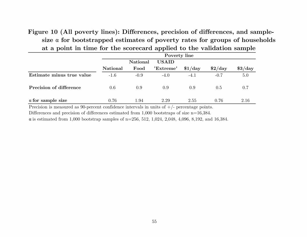
55

Figure 10 (All poverty lines): Differences, precision of differences, and sample-size α for bootstrapped estimates of poverty rates for groups of households at a point in time for the scorecard applied to the validation sample

National USAIDNational Food 'Extreme' $1/day $2/day $3/day

Estimate minus true value -1.6 -0.9 -4.0 -4.1 -0.7 5.0

Precision of difference 0.6 0.9 0.9 0.9 0.5 0.7

α for sample size 0.76 1.94 2.29 2.55 0.76 2.16Precision is measured as 90-percent confidence intervals in units of +/- percentage points. Differences and precision of differences estimated from 1,000 bootstraps of size n=16,384.α is estimated from 1,000 bootstrap samples of n=256, 512, 1,024, 2,048, 4,096, 8,192, and 16,384.

Poverty line

56

Figure 11 (National poverty line): Differences and precision of differences for bootstrapped estimates of poverty rates for groups of households at a point in time, by sample size, scorecard applied to the validation sample

Sample size (n) Diff. 90-percent 95-percent 99-percent2 -0.3 48.9 60.3 72.04 0.1 33.6 41.6 55.28 -0.8 24.3 29.4 39.416 -1.2 17.2 19.8 26.832 -1.3 12.2 14.6 19.664 -1.3 8.6 10.1 13.0128 -1.4 6.1 7.1 8.8256 -1.5 4.4 5.2 6.9512 -1.6 3.2 3.8 4.9

1,024 -1.5 2.1 2.6 3.72,048 -1.6 1.6 1.9 2.44,096 -1.6 1.1 1.3 1.78,192 -1.6 0.8 0.9 1.216,384 -1.6 0.6 0.7 0.9

Difference between estimate and true valueConfidence interval (+/- percentage points)

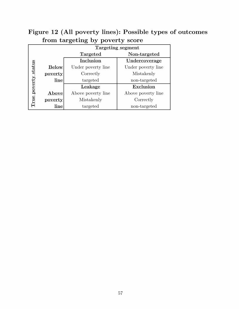
57

Figure 12 (All poverty lines): Possible types of outcomes from targeting by poverty score

Targeted Non-targetedInclusion Undercoverage

Below Under poverty line Under poverty linepoverty Correctly Mistakenly

line targeted non-targetedLeakage Exclusion

Above Above poverty line Above poverty linepoverty Mistakenly Correctly

line targeted non-targeted

Targeting segment

Tru

e po

vert

y st

atus

58

Figure 13 (National poverty line): Households by targeting classification and score, along with “Total Accuracy” and BPAC, scorecard applied to the validation sample

Inclusion: Undercoverage: Leakage: Exclusion: Total Accuracy BPAC< poverty line < poverty line ≥ poverty line ≥ poverty line Inclusion

correctly mistakenly mistakenly correctly +Score targeted non-targeted targeted non-targeted Exclusion0–4 0.3 58.1 0.0 41.6 41.9 -99.05–9 0.6 57.8 0.0 41.6 42.2 -98.0

10–14 3.1 55.3 0.1 41.5 44.6 -89.315–19 6.7 51.6 0.2 41.5 48.2 -76.720–24 10.2 48.2 0.5 41.1 51.3 -64.225–29 19.5 38.9 1.9 39.8 59.3 -30.030–34 26.9 31.5 2.7 39.0 65.8 -3.335–39 37.5 20.9 5.6 36.0 73.5 38.040–44 46.1 12.3 8.4 33.2 79.3 72.445–49 49.3 9.1 11.3 30.3 79.6 80.650–54 53.1 5.2 15.5 26.1 79.3 73.455–59 55.6 2.8 21.8 19.9 75.4 62.660–64 57.4 1.0 26.0 15.6 73.0 55.465–69 57.9 0.4 30.8 10.9 68.8 47.370–74 58.0 0.3 35.1 6.6 64.6 39.975–79 58.2 0.1 37.8 3.8 62.0 35.280–84 58.2 0.1 40.2 1.4 59.7 31.185–89 58.4 0.0 40.9 0.7 59.1 29.990–94 58.4 0.0 41.4 0.3 58.6 29.195–100 58.4 0.0 41.6 0.0 58.4 28.6

See text

Inclusion, undercoverage, leakage, and exclusion normalized to sum to 100.

59

Figure 14 (National poverty line): Households below the poverty line and all households, at a given score or at or below a given score cut-off, scorecard applied to the validation sample

Score At score At or below score At score At or below score0–4 100.0 100.0 0.3 0.35–9 100.0 100.0 0.3 0.6

10–14 96.1 96.8 2.6 3.215–19 97.9 97.4 3.7 6.920–24 90.8 95.1 3.8 10.725–29 87.4 91.2 10.6 21.430–34 90.1 90.9 8.2 29.635–39 78.1 86.9 13.5 43.140–44 75.5 84.5 11.4 54.545–49 53.0 81.3 6.1 60.650–54 47.8 77.4 8.0 68.655–59 28.1 71.8 8.8 77.460–64 29.4 68.8 6.0 83.465–69 11.0 65.3 5.3 88.770–74 1.8 62.3 4.4 93.175–79 6.5 60.6 3.0 96.080–84 0.6 59.2 2.4 98.485–89 15.3 58.8 0.8 99.390–94 0.0 58.5 0.5 99.795–100 0.0 58.4 0.3 100.0

People below poverty line (%) All people (%)

60

National Food Poverty Line Tables

61

Figure 4 (National Food poverty line): Estimated poverty likelihoods associated with scores

If an individual's score is . . .. . . then the likelihood (%) of being

below the poverty line is:0–4 72.85–9 86.9

10–14 81.015–19 76.820–24 77.825–29 71.730–34 75.035–39 45.140–44 45.845–49 36.050–54 19.055–59 8.560–64 5.065–69 0.970–74 0.475–79 0.080–84 0.885–89 0.090–94 0.095–100 0.0

Surveyed cases weighted to represent Mali's households.Based on the 2001 EMEP.

62

Figure 5 (National Food poverty line): Derivation of estimated poverty likelihoods associated with scores

People below All people Poverty likelihoodScore poverty line at score (estimated, %)0–4 208 ÷ 286 = 72.85–9 262 ÷ 302 = 86.9

10–14 2,092 ÷ 2,582 = 81.015–19 2,859 ÷ 3,725 = 76.820–24 2,976 ÷ 3,825 = 77.825–29 7,625 ÷ 10,638 = 71.730–34 6,157 ÷ 8,210 = 75.035–39 6,105 ÷ 13,527 = 45.140–44 5,226 ÷ 11,414 = 45.845–49 2,195 ÷ 6,093 = 36.050–54 1,525 ÷ 8,033 = 19.055–59 745 ÷ 8,760 = 8.560–64 301 ÷ 5,975 = 5.065–69 46 ÷ 5,327 = 0.970–74 18 ÷ 4,386 = 0.475–79 0 ÷ 2,965 = 0.080–84 19 ÷ 2,379 = 0.885–89 0 ÷ 846 = 0.090–94 0 ÷ 477 = 0.095–100 0 ÷ 251 = 0.0Surveyed cases weighted to represent Mali's households.Based on the 2001 EMEP.

63

Figure 7 (National Food poverty line): Bootstrapped differences between estimated and true poverty likelihoods for households in a large sample (n = 16,384), with confidence intervals, scorecard applied to the validation sample

Score Diff. 90-percent 95-percent 99-percent0–4 48.3 9.0 10.7 14.65–9 11.4 11.7 13.5 19.0

10–14 28.1 5.8 6.9 8.915–19 -13.8 7.8 8.0 8.320–24 6.6 3.6 4.4 5.825–29 2.0 2.2 2.6 3.630–34 -12.1 6.7 6.9 7.135–39 7.0 2.5 3.0 3.840–44 -7.7 5.4 5.6 6.345–49 7.3 2.8 3.3 4.350–54 -6.2 4.2 4.4 4.855–59 3.9 0.7 0.8 1.060–64 -1.9 1.7 1.8 2.265–69 -1.6 1.3 1.3 1.570–74 0.3 0.1 0.1 0.175–79 -2.7 1.9 2.1 2.280–84 0.7 0.1 0.1 0.185–89 0.0 0.0 0.0 0.090–94 0.0 0.0 0.0 0.095–100 0.0 0.0 0.0 0.0

Confidence interval (+/- percentage points)

Scorecard applied to validation sample,difference between estimate and true value

64

Figure 9 (National Food poverty line): Differences and precision of differences for bootstrapped estimates of households’ poverty likelihoods, by sample size, scorecard applied to the validation sample

Sample size (n) Diff. 90-percent 95-percent 99-percent2 -0.7 51.1 58.9 73.54 0.2 41.1 46.9 61.28 -0.7 32.8 37.5 45.816 -0.2 25.5 29.0 36.332 -0.6 18.5 22.7 27.164 0.0 13.3 15.3 19.1128 0.1 8.6 10.0 12.4256 0.4 6.4 7.9 10.1512 0.7 4.6 5.3 7.3

1,024 0.9 3.4 4.2 5.22,048 1.1 2.4 2.8 4.04,096 1.2 1.6 2.0 2.58,192 1.1 1.2 1.4 1.816,384 1.1 0.9 1.0 1.3

Confidence interval (+/- percentage points)Difference between estimate and true value

65

Figure 11 (National Food poverty line): Differences and precision of differences for bootstrapped estimates of poverty rates for groups of households at a point in time, by sample size, scorecard applied to the validation sample

Sample size (n) Diff. 90-percent 95-percent 99-percent2 -0.7 51.1 58.9 73.54 -0.1 40.6 47.2 60.68 -1.1 32.7 37.9 44.416 -0.7 25.5 29.1 34.332 -1.1 17.9 21.6 27.464 -0.8 12.5 14.7 19.0128 -0.8 9.0 10.5 14.6256 -0.9 7.0 8.2 11.2512 -0.9 4.8 5.7 7.6

1,024 -0.9 3.4 4.0 5.22,048 -0.9 2.4 2.9 3.84,096 -0.9 1.7 2.0 2.78,192 -0.9 1.2 1.4 2.016,384 -0.9 0.9 1.0 1.4

Difference between estimate and true valueConfidence interval (+/- percentage points)

66

Figure 13 (National Food poverty line): Households by targeting classification and score, along with “Total Accuracy” and BPAC, scorecard applied to the validation sample

Inclusion: Undercoverage: Leakage: Exclusion: Total Accuracy BPAC< poverty line < poverty line ? poverty line ? poverty line Inclusion

correctly mistakenly mistakenly correctly +Score targeted non-targeted targeted non-targeted Exclusion0–4 0.1 40.0 0.1 59.7 59.8 -98.95–9 0.4 39.8 0.2 59.6 60.0 -97.6

10–14 2.4 37.8 0.8 59.0 61.4 -86.115–19 5.6 34.6 1.3 58.5 64.2 -68.820–24 8.4 31.8 2.3 57.5 65.9 -52.525–29 16.1 24.1 5.3 54.5 70.6 -6.930–34 21.9 18.3 7.7 52.1 74.0 28.135–39 29.3 10.9 13.8 46.0 75.3 65.740–44 34.4 5.8 20.1 39.7 74.1 50.045–49 36.3 3.9 24.3 35.5 71.7 39.550–54 38.4 1.8 30.2 29.6 67.9 24.755–59 39.5 0.7 37.9 21.9 61.3 5.660–64 39.9 0.3 43.4 16.4 56.3 -8.165–69 40.1 0.1 48.6 11.2 51.2 -21.070–74 40.1 0.1 53.0 6.8 46.9 -31.975–79 40.2 0.0 55.9 3.9 44.1 -39.080–84 40.2 0.0 58.2 1.6 41.8 -44.985–89 40.2 0.0 59.1 0.7 40.9 -47.090–94 40.2 0.0 59.6 0.3 40.4 -48.295–100 40.2 0.0 59.8 0.0 40.2 -48.8

See text

Inclusion, undercoverage, leakage, and exclusion normalized to sum to 100.

67

Figure 14 (National Food poverty line): Households below the poverty line and all households, at a given score or at or below a given score cut-off, scorecard applied to the validation sample

Score At score At or below score At score At or below score0–4 49.2 49.2 0.3 0.35–9 79.1 64.6 0.3 0.6

10–14 78.4 75.8 2.6 3.215–19 86.6 81.6 3.7 6.920–24 72.0 78.2 3.8 10.725–29 72.1 75.2 10.6 21.430–34 71.1 74.1 8.2 29.635–39 54.8 68.0 13.5 43.140–44 44.6 63.1 11.4 54.545–49 30.6 59.8 6.1 60.650–54 26.4 55.9 8.0 68.655–59 12.2 51.0 8.8 77.460–64 7.9 47.9 6.0 83.465–69 2.7 45.2 5.3 88.770–74 0.4 43.1 4.4 93.175–79 3.1 41.8 3.0 96.080–84 0.6 40.8 2.4 98.485–89 0.0 40.5 0.8 99.390–94 0.0 40.3 0.5 99.795–100 0.0 40.2 0.3 100.0

People below poverty line (%) All people (%)

68

USAID “Extreme” Poverty Line Tables

69

Figure 4 (USAID “Extreme” poverty line): Estimated poverty likelihoods associated with scores

If an individual's score is . . .. . . then the likelihood (%) of being

below the poverty line is:0–4 72.85–9 86.9

10–14 74.715–19 72.120–24 70.325–29 59.730–34 61.435–39 26.740–44 30.645–49 18.150–54 11.255–59 4.060–64 2.265–69 0.570–74 0.475–79 0.080–84 0.085–89 0.090–94 0.095–100 0.0

Surveyed cases weighted to represent Mali's households.Based on the 2001 EMEP.

70

Figure 5 (USAID “Extreme” poverty line): Derivation of estimated poverty likelihoods associated with scores

People below All people Poverty likelihoodScore poverty line at score (estimated, %)0–4 208 ÷ 286 = 72.85–9 262 ÷ 302 = 86.9

10–14 1,928 ÷ 2,582 = 74.715–19 2,685 ÷ 3,725 = 72.120–24 2,689 ÷ 3,825 = 70.325–29 6,350 ÷ 10,638 = 59.730–34 5,038 ÷ 8,210 = 61.435–39 3,610 ÷ 13,527 = 26.740–44 3,487 ÷ 11,414 = 30.645–49 1,105 ÷ 6,093 = 18.150–54 898 ÷ 8,033 = 11.255–59 352 ÷ 8,760 = 4.060–64 131 ÷ 5,975 = 2.265–69 25 ÷ 5,327 = 0.570–74 18 ÷ 4,386 = 0.475–79 0 ÷ 2,965 = 0.080–84 0 ÷ 2,379 = 0.085–89 0 ÷ 846 = 0.090–94 0 ÷ 477 = 0.095–100 0 ÷ 251 = 0.0Surveyed cases weighted to represent Mali's households.Based on the 2001 EMEP.

71

Figure 7 (USAID “Extreme” poverty line): Bootstrapped differences between estimated and true poverty likelihoods for households in a large sample (n = 16,384), with confidence intervals, scorecard applied to the validation sample

Score Diff. 90-percent 95-percent 99-percent0–4 48.3 9.0 10.7 14.65–9 11.4 11.7 13.5 19.0

10–14 24.1 5.8 6.5 8.615–19 -12.0 7.2 7.4 7.920–24 4.2 3.7 4.6 5.925–29 3.6 2.5 3.0 4.030–34 -17.9 9.9 10.0 10.335–39 5.5 1.7 1.9 2.740–44 -17.5 10.3 10.6 11.245–49 5.1 1.7 2.1 2.650–54 -6.7 4.3 4.5 5.055–59 2.3 0.4 0.5 0.660–64 0.0 0.7 0.9 1.265–69 0.5 0.0 0.0 0.070–74 0.3 0.1 0.1 0.175–79 0.0 0.0 0.0 0.080–84 0.0 0.0 0.0 0.085–89 0.0 0.0 0.0 0.090–94 0.0 0.0 0.0 0.095–100 0.0 0.0 0.0 0.0

Scorecard applied to validation sample,difference between estimate and true value

Confidence interval (+/- percentage points)

72

Figure 9 (USAID “Extreme” poverty line): Differences and precision of differences for bootstrapped estimates of households’ poverty likelihoods, by sample size, scorecard applied to the validation sample

Sample size (n) Diff. 90-percent 95-percent 99-percent2 -1.2 51.2 60.9 71.34 -1.0 38.7 46.8 58.98 -1.8 32.0 37.6 47.416 -2.6 24.9 30.2 36.932 -3.4 19.0 22.7 28.264 -3.1 13.2 15.8 19.7128 -2.9 8.8 10.3 13.4256 -2.5 6.2 7.7 10.5512 -2.1 4.6 5.4 7.3

1,024 -1.8 3.4 4.0 5.42,048 -1.6 2.4 2.9 4.14,096 -1.6 1.7 2.0 2.78,192 -1.6 1.3 1.5 1.916,384 -1.6 0.9 1.0 1.3

Difference between estimate and true valueConfidence interval (+/- percentage points)

73

Figure 11 (USAID “Extreme” poverty line): Differences and precision of differences for bootstrapped estimates of poverty rates for groups of households at a point in time, by sample size, scorecard applied to the validation sample

Sample size (n) Diff. 90-percent 95-percent 99-percent2 -1.2 51.2 60.9 71.34 -1.2 38.8 47.1 58.38 -2.2 32.0 37.0 45.416 -2.8 24.5 28.6 35.332 -3.5 18.1 21.3 26.164 -3.6 12.3 14.9 19.7128 -3.8 9.5 11.0 14.0256 -3.9 6.8 8.1 10.3512 -3.8 4.8 5.9 7.6

1,024 -3.9 3.4 4.1 5.22,048 -3.9 2.3 2.9 3.94,096 -3.9 1.8 2.1 2.78,192 -3.9 1.3 1.5 1.916,384 -4.0 0.9 1.1 1.3

Difference between estimate and true valueConfidence interval (+/- percentage points)

74

Figure 13 (USAID “Extreme” poverty line): Households by targeting classification and score, along with “Total Accuracy” and BPAC, scorecard applied to the validation sample

Inclusion: Undercoverage: Leakage: Exclusion: Total Accuracy BPAC< poverty line < poverty line ? poverty line ? poverty line Inclusion

correctly mistakenly mistakenly correctly +Score targeted non-targeted targeted non-targeted Exclusion0–4 0.1 30.4 0.1 69.3 69.4 -98.65–9 0.4 30.2 0.2 69.2 69.6 -96.8

10–14 2.3 28.3 0.9 68.6 70.9 -82.115–19 5.2 25.3 1.7 67.8 73.0 -60.320–24 7.7 22.9 3.1 66.4 74.1 -39.825–29 14.0 16.5 7.3 62.1 76.1 15.830–34 18.6 11.9 11.0 58.5 77.1 57.735–39 23.9 6.6 19.1 50.3 74.2 37.340–44 27.4 3.2 27.1 42.3 69.7 11.245–49 28.5 2.1 32.1 37.3 65.8 -5.250–54 29.9 0.7 38.8 30.7 60.6 -26.955–59 30.3 0.2 47.1 22.4 52.7 -54.160–64 30.5 0.0 52.8 16.6 47.1 -73.065–69 30.5 0.0 58.2 11.3 41.8 -90.470–74 30.5 0.0 62.5 6.9 37.5 -104.775–79 30.5 0.0 65.5 4.0 34.5 -114.480–84 30.5 0.0 67.9 1.6 32.1 -122.285–89 30.5 0.0 68.7 0.7 31.3 -125.090–94 30.5 0.0 69.2 0.3 30.8 -126.695–100 30.5 0.0 69.5 0.0 30.5 -127.4Inclusion, undercoverage, leakage, and exclusion normalized to sum to 100.

See text

75

Figure 14 (USAID “Extreme” poverty line): Households below the poverty line and all households, at a given score or at or below a given score cut-off, scorecard applied to the validation sample

Score At score At or below score At score At or below score0–4 49.2 49.2 0.3 0.35–9 79.1 64.6 0.3 0.6

10–14 74.2 72.4 2.6 3.215–19 79.0 76.0 3.7 6.920–24 63.4 71.5 3.8 10.725–29 59.8 65.7 10.6 21.430–34 55.8 62.9 8.2 29.635–39 39.5 55.6 13.5 43.140–44 30.0 50.2 11.4 54.545–49 18.0 47.0 6.1 60.650–54 17.5 43.5 8.0 68.655–59 5.0 39.2 8.8 77.460–64 3.6 36.6 6.0 83.465–69 0.1 34.4 5.3 88.770–74 0.4 32.8 4.4 93.175–79 0.0 31.8 3.0 96.080–84 0.0 31.0 2.4 98.485–89 0.0 30.8 0.8 99.390–94 0.0 30.6 0.5 99.795–100 0.0 30.5 0.3 100.0

People below poverty line (%) All people (%)

76

$1/Day Poverty Line Tables

77

Figure 4 ($1/Day poverty line): Estimated poverty likelihoods associated with scores

If an individual's score is . . .. . . then the likelihood (%) of being

below the poverty line is:0–4 72.85–9 86.9

10–14 71.215–19 66.820–24 60.425–29 50.330–34 58.335–39 25.840–44 27.245–49 13.050–54 10.255–59 3.560–64 0.865–69 0.070–74 0.475–79 0.080–84 0.085–89 0.090–94 0.095–100 0.0

Surveyed cases weighted to represent Mali's households.Based on the 2001 EMEP.

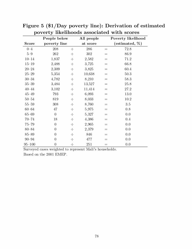
78

Figure 5 ($1/Day poverty line): Derivation of estimated poverty likelihoods associated with scores

People below All people Poverty likelihoodScore poverty line at score (estimated, %)0–4 208 ÷ 286 = 72.85–9 262 ÷ 302 = 86.9

10–14 1,837 ÷ 2,582 = 71.215–19 2,488 ÷ 3,725 = 66.820–24 2,309 ÷ 3,825 = 60.425–29 5,354 ÷ 10,638 = 50.330–34 4,782 ÷ 8,210 = 58.335–39 3,484 ÷ 13,527 = 25.840–44 3,102 ÷ 11,414 = 27.245–49 793 ÷ 6,093 = 13.050–54 819 ÷ 8,033 = 10.255–59 308 ÷ 8,760 = 3.560–64 47 ÷ 5,975 = 0.865–69 0 ÷ 5,327 = 0.070–74 18 ÷ 4,386 = 0.475–79 0 ÷ 2,965 = 0.080–84 0 ÷ 2,379 = 0.085–89 0 ÷ 846 = 0.090–94 0 ÷ 477 = 0.095–100 0 ÷ 251 = 0.0Surveyed cases weighted to represent Mali's households.Based on the 2001 EMEP.

79

Figure 7 ($1/Day poverty line): Bootstrapped differences between estimated and true poverty likelihoods for households in a large sample (n = 16,384), with confidence intervals, scorecard applied to the validation sample

Score Diff. 90-percent 95-percent 99-percent0–4 48.3 9.0 10.7 14.65–9 11.4 11.7 13.5 19.0

10–14 21.5 5.7 6.5 8.515–19 -12.6 7.7 8.0 8.620–24 1.8 3.7 4.6 6.325–29 7.4 2.3 2.8 3.830–34 -20.9 11.4 11.5 11.835–39 6.8 1.5 1.9 2.640–44 -17.1 10.1 10.3 10.945–49 1.0 1.7 2.0 2.550–54 -6.1 4.0 4.2 4.655–59 2.2 0.3 0.4 0.560–64 -1.0 0.9 0.9 1.165–69 0.0 0.0 0.0 0.070–74 0.3 0.1 0.1 0.175–79 0.0 0.0 0.0 0.080–84 0.0 0.0 0.0 0.085–89 0.0 0.0 0.0 0.090–94 0.0 0.0 0.0 0.095–100 0.0 0.0 0.0 0.0

difference between estimate and true valueConfidence interval (+/- percentage points)

Scorecard applied to validation sample,

80

Figure 9 ($1/Day poverty line): Differences and precision of differences for bootstrapped estimates of households’ poverty likelihoods, by sample size, scorecard applied to the validation sample

Sample size (n) Diff. 90-percent 95-percent 99-percent2 -1.0 50.4 59.7 68.94 -0.5 37.0 47.5 57.08 -1.6 32.8 38.2 48.216 -2.7 25.5 30.7 36.032 -3.8 19.4 21.9 28.364 -3.6 13.4 15.7 19.6128 -3.4 9.0 10.5 14.2256 -3.0 6.3 7.8 10.7512 -2.5 4.7 5.6 7.6

1,024 -2.2 3.5 4.1 5.22,048 -2.1 2.4 2.9 4.14,096 -2.0 1.7 2.0 2.78,192 -2.1 1.3 1.5 2.016,384 -2.1 0.9 1.0 1.3

Difference between estimate and true valueConfidence interval (+/- percentage points)

81

Figure 11 ($1/Day poverty line): Differences and precision of differences for bootstrapped estimates of poverty rates for groups of households at a point in time, by sample size, scorecard applied to the validation sample

Sample size (n) Diff. 90-percent 95-percent 99-percent2 -1.0 50.4 59.7 68.94 -0.7 37.5 47.7 56.68 -1.7 32.0 37.2 46.116 -2.6 25.4 28.7 35.432 -3.5 18.3 21.4 27.064 -3.6 13.0 15.2 20.1128 -3.9 9.6 11.4 14.1256 -4.0 7.0 8.5 10.7512 -4.0 4.9 5.9 7.7

1,024 -4.0 3.5 4.1 5.42,048 -4.0 2.4 2.9 4.24,096 -4.0 1.8 2.1 2.78,192 -4.1 1.3 1.6 1.916,384 -4.1 0.9 1.1 1.4

Difference between estimate and true valueConfidence interval (+/- percentage points)

82

Figure 13 ($1/Day poverty line): Households by targeting classification and score, along with “Total Accuracy” and BPAC, scorecard applied to the validation sample

Inclusion: Undercoverage: Leakage: Exclusion: Total Accuracy BPAC< poverty line < poverty line ? poverty line ? poverty line Inclusion

correctly mistakenly mistakenly correctly +Score targeted non-targeted targeted non-targeted Exclusion0–4 0.1 27.0 0.1 72.8 72.9 -98.45–9 0.4 26.7 0.2 72.7 73.1 -96.4

10–14 2.2 24.9 0.9 72.0 74.2 -80.015–19 5.0 22.1 1.8 71.1 76.1 -55.920–24 7.1 20.0 3.6 69.3 76.5 -34.125–29 12.5 14.6 8.9 64.0 76.5 24.930–34 17.0 10.1 12.6 60.3 77.3 53.635–39 21.7 5.4 21.4 51.5 73.2 21.140–44 24.3 2.8 30.2 42.7 67.0 -11.445–49 25.3 1.8 35.3 37.6 63.0 -30.250–54 26.6 0.5 42.1 30.8 57.4 -55.255–59 26.9 0.2 50.5 22.4 49.3 -86.360–64 27.1 0.0 56.3 16.6 43.7 -107.765–69 27.1 0.0 61.6 11.3 38.4 -127.470–74 27.1 0.0 66.0 6.9 34.0 -143.575–79 27.1 0.0 68.9 4.0 31.1 -154.480–84 27.1 0.0 71.3 1.6 28.7 -163.285–89 27.1 0.0 72.2 0.7 27.8 -166.390–94 27.1 0.0 72.7 0.3 27.3 -168.195–100 27.1 0.0 72.9 0.0 27.1 -169.0Inclusion, undercoverage, leakage, and exclusion normalized to sum to 100.

See text

83

Figure 14 ($1/Day poverty line): Households below the poverty line and all households, at a given score or at or below a given score cut-off, scorecard applied to the validation sample

Score At score At or below score At score At or below score0–4 49.2 49.2 0.3 0.35–9 79.1 64.6 0.3 0.6

10–14 71.9 70.6 2.6 3.215–19 75.4 73.2 3.7 6.920–24 54.9 66.7 3.8 10.725–29 50.1 58.4 10.6 21.430–34 54.9 57.4 8.2 29.635–39 34.9 50.4 13.5 43.140–44 22.9 44.6 11.4 54.545–49 16.5 41.8 6.1 60.650–54 15.5 38.7 8.0 68.655–59 3.8 34.8 8.8 77.460–64 2.9 32.5 6.0 83.465–69 0.1 30.5 5.3 88.770–74 0.4 29.1 4.4 93.175–79 0.0 28.2 3.0 96.080–84 0.0 27.5 2.4 98.485–89 0.0 27.3 0.8 99.390–94 0.0 27.2 0.5 99.795–100 0.0 27.1 0.3 100.0

People below poverty line (%) All people (%)

84

$2/Day Poverty Line Tables

85

Figure 4 ($2/Day poverty line): Estimated poverty likelihoods associated with scores

If an individual's score is . . .. . . then the likelihood (%) of being

below the poverty line is:0–4 100.05–9 86.9

10–14 99.515–19 96.720–24 94.525–29 92.630–34 90.535–39 83.640–44 85.445–49 70.550–54 57.355–59 30.460–64 26.065–69 7.470–74 8.375–79 7.880–84 0.885–89 0.090–94 5.995–100 0.0

Surveyed cases weighted to represent Mali's households.Based on the 2001 EMEP.

86

Figure 5 ($2/Day poverty line): Derivation of estimated poverty likelihoods associated with scores

People below All people Poverty likelihoodScore poverty line at score (estimated, %)0–4 286 ÷ 286 = 100.05–9 262 ÷ 302 = 86.9

10–14 2,568 ÷ 2,582 = 99.515–19 3,601 ÷ 3,725 = 96.720–24 3,614 ÷ 3,825 = 94.525–29 9,853 ÷ 10,638 = 92.630–34 7,431 ÷ 8,210 = 90.535–39 11,307 ÷ 13,527 = 83.640–44 9,751 ÷ 11,414 = 85.445–49 4,293 ÷ 6,093 = 70.550–54 4,606 ÷ 8,033 = 57.355–59 2,660 ÷ 8,760 = 30.460–64 1,553 ÷ 5,975 = 26.065–69 392 ÷ 5,327 = 7.470–74 365 ÷ 4,386 = 8.375–79 232 ÷ 2,965 = 7.880–84 19 ÷ 2,379 = 0.885–89 0 ÷ 846 = 0.090–94 28 ÷ 477 = 5.995–100 0 ÷ 251 = 0.0Surveyed cases weighted to represent Mali's households.Based on the 2001 EMEP.

87

Figure 7 ($2/Day poverty line): Bootstrapped differences between estimated and true poverty likelihoods for households in a large sample (n = 16,384), with confidence intervals, scorecard applied to the validation sample

Score Diff. 90-percent 95-percent 99-percent0–4 0.0 0.0 0.0 0.05–9 -13.1 6.6 6.6 6.6

10–14 -0.2 0.2 0.3 0.415–19 -2.5 1.4 1.5 1.520–24 8.7 3.3 3.9 4.925–29 3.8 1.4 1.7 2.230–34 -6.6 3.5 3.6 3.735–39 -5.6 3.4 3.5 3.840–44 -7.3 4.1 4.1 4.245–49 9.6 3.3 3.8 5.150–54 2.0 2.4 3.0 4.155–59 14.5 1.7 2.0 2.760–64 -12.5 7.8 8.1 8.865–69 -1.8 1.7 1.9 2.370–74 1.6 1.5 1.9 2.475–79 0.2 1.9 2.2 2.980–84 0.7 0.1 0.1 0.185–89 -37.3 23.3 24.0 25.290–94 5.9 0.0 0.0 0.095–100 0.0 0.0 0.0 0.0

Scorecard applied to validation sample,difference between estimate and true value

Confidence interval (+/- percentage points)

88

Figure 9 ($2/Day poverty line): Differences and precision of differences for bootstrapped estimates of households’ poverty likelihoods, by sample size, scorecard applied to the validation sample

Sample size (n) Diff. 90-percent 95-percent 99-percent2 -0.5 49.2 59.1 73.14 -0.3 34.5 41.8 56.78 -0.9 23.2 29.7 41.816 -1.0 17.0 20.9 27.432 -0.5 12.8 15.5 20.264 -0.2 8.7 10.6 13.3128 -0.2 5.9 7.2 9.5256 -0.4 4.5 5.3 6.6512 -0.6 3.2 3.9 5.0

1,024 -0.6 2.2 2.5 3.32,048 -0.7 1.5 1.9 2.34,096 -0.6 1.1 1.3 1.88,192 -0.6 0.7 0.9 1.316,384 -0.6 0.6 0.7 0.8

Difference between estimate and true valueConfidence interval (+/- percentage points)

89

Figure 11 ($2/Day poverty line): Differences and precision of differences for bootstrapped estimates of poverty rates for groups of households at a point in time, by sample size, scorecard applied to the validation sample

Sample size (n) Diff. 90-percent 95-percent 99-percent2 -0.5 49.2 59.1 73.14 -0.4 33.2 40.2 57.98 -0.8 22.9 28.9 40.216 -0.9 16.5 19.6 25.032 -0.7 11.9 14.0 19.564 -0.6 8.4 10.1 13.1128 -0.6 5.8 7.1 9.8256 -0.7 4.3 5.2 6.9512 -0.7 3.2 3.9 5.0

1,024 -0.7 2.1 2.5 3.62,048 -0.7 1.6 1.8 2.34,096 -0.7 1.1 1.3 1.78,192 -0.7 0.8 0.9 1.316,384 -0.7 0.5 0.6 0.9

Difference between estimate and true valueConfidence interval (+/- percentage points)

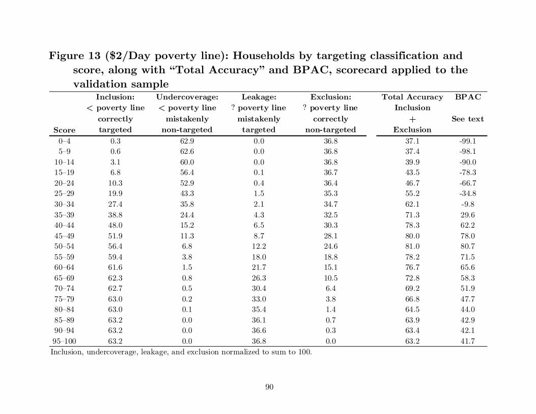
90

Figure 13 ($2/Day poverty line): Households by targeting classification and score, along with “Total Accuracy” and BPAC, scorecard applied to the validation sample

Inclusion: Undercoverage: Leakage: Exclusion: Total Accuracy BPAC< poverty line < poverty line ? poverty line ? poverty line Inclusion

correctly mistakenly mistakenly correctly +Score targeted non-targeted targeted non-targeted Exclusion0–4 0.3 62.9 0.0 36.8 37.1 -99.15–9 0.6 62.6 0.0 36.8 37.4 -98.1

10–14 3.1 60.0 0.0 36.8 39.9 -90.015–19 6.8 56.4 0.1 36.7 43.5 -78.320–24 10.3 52.9 0.4 36.4 46.7 -66.725–29 19.9 43.3 1.5 35.3 55.2 -34.830–34 27.4 35.8 2.1 34.7 62.1 -9.835–39 38.8 24.4 4.3 32.5 71.3 29.640–44 48.0 15.2 6.5 30.3 78.3 62.245–49 51.9 11.3 8.7 28.1 80.0 78.050–54 56.4 6.8 12.2 24.6 81.0 80.755–59 59.4 3.8 18.0 18.8 78.2 71.560–64 61.6 1.5 21.7 15.1 76.7 65.665–69 62.3 0.8 26.3 10.5 72.8 58.370–74 62.7 0.5 30.4 6.4 69.2 51.975–79 63.0 0.2 33.0 3.8 66.8 47.780–84 63.0 0.1 35.4 1.4 64.5 44.085–89 63.2 0.0 36.1 0.7 63.9 42.990–94 63.2 0.0 36.6 0.3 63.4 42.195–100 63.2 0.0 36.8 0.0 63.2 41.7Inclusion, undercoverage, leakage, and exclusion normalized to sum to 100.

See text

91

Figure 14 ($2/Day poverty line): Households below the poverty line and all households, at a given score or at or below a given score cut-off, scorecard applied to the validation sample

Score At score At or below score At score At or below score0–4 100.0 100.0 0.3 0.35–9 100.0 100.0 0.3 0.6

10–14 98.9 99.1 2.6 3.215–19 97.9 98.5 3.7 6.920–24 92.2 96.2 3.8 10.725–29 89.7 93.0 10.6 21.430–34 92.2 92.8 8.2 29.635–39 84.0 90.0 13.5 43.140–44 80.6 88.1 11.4 54.545–49 63.9 85.6 6.1 60.650–54 56.4 82.2 8.0 68.655–59 34.1 76.8 8.8 77.460–64 37.3 73.9 6.0 83.465–69 13.2 70.3 5.3 88.770–74 8.3 67.4 4.4 93.175–79 10.6 65.6 3.0 96.080–84 0.6 64.1 2.4 98.485–89 17.2 63.7 0.8 99.390–94 0.0 63.3 0.5 99.795–100 0.0 63.2 0.3 100.0

People below poverty line (%) All people (%)

92

$3/Day Poverty Line Tables

93

Figure 4 ($3/Day poverty line): Estimated poverty likelihoods associated with scores

If an individual's score is . . .. . . then the likelihood (%) of being

below the poverty line is:0–4 100.05–9 100.0

10–14 100.015–19 100.020–24 99.625–29 97.930–34 98.535–39 90.640–44 95.945–49 91.550–54 88.755–59 68.760–64 55.165–69 59.170–74 42.075–79 26.480–84 38.285–89 39.090–94 10.095–100 0.0

Surveyed cases weighted to represent Mali's households.Based on the 2001 EMEP.

94

Figure 5 ($3/Day poverty line): Derivation of estimated poverty likelihoods associated with scores

People below All people Poverty likelihoodScore poverty line at score (estimated, %)0–4 286 ÷ 286 = 100.05–9 302 ÷ 302 = 100.0

10–14 2,582 ÷ 2,582 = 100.015–19 3,725 ÷ 3,725 = 100.020–24 3,808 ÷ 3,825 = 99.625–29 10,411 ÷ 10,638 = 97.930–34 8,084 ÷ 8,210 = 98.535–39 12,259 ÷ 13,527 = 90.640–44 10,943 ÷ 11,414 = 95.945–49 5,573 ÷ 6,093 = 91.550–54 7,126 ÷ 8,033 = 88.755–59 6,019 ÷ 8,760 = 68.760–64 3,290 ÷ 5,975 = 55.165–69 3,147 ÷ 5,327 = 59.170–74 1,842 ÷ 4,386 = 42.075–79 783 ÷ 2,965 = 26.480–84 909 ÷ 2,379 = 38.285–89 329 ÷ 846 = 39.090–94 48 ÷ 477 = 10.095–100 0 ÷ 251 = 0.0Surveyed cases weighted to represent Mali's households.Based on the 2001 EMEP.

95

Figure 7 ($3/Day poverty line): Bootstrapped differences between estimated and true poverty likelihoods for households in a large sample (n = 16,384), with confidence intervals, scorecard applied to the validation sample

Score Diff. 90-percent 95-percent 99-percent0–4 0.0 0.0 0.0 0.05–9 0.0 0.0 0.0 0.0

10–14 0.0 0.0 0.0 0.015–19 0.5 0.3 0.4 0.520–24 0.4 0.4 0.5 0.725–29 -0.2 0.6 0.7 0.930–34 0.1 0.4 0.5 0.735–39 -4.9 2.8 2.9 3.140–44 -1.0 0.8 0.8 0.945–49 0.5 1.6 1.9 2.650–54 -0.2 1.5 1.8 2.355–59 41.0 2.3 2.9 3.760–64 -9.1 6.2 6.4 7.065–69 18.4 3.2 3.8 5.170–74 5.0 3.6 4.5 5.875–79 -1.8 4.1 5.0 6.980–84 -11.7 8.3 8.7 9.785–89 -4.6 9.0 10.6 13.690–94 -25.9 18.1 18.6 20.495–100 -29.7 21.3 22.6 25.5

difference between estimate and true valueConfidence interval (+/- percentage points)

Scorecard applied to validation sample,

96

Figure 9 ($3/Day poverty line): Differences and precision of differences for bootstrapped estimates of households’ poverty likelihoods, by sample size, scorecard applied to the validation sample

Sample size (n) Diff. 90-percent 95-percent 99-percent2 1.6 44.5 53.2 68.14 2.2 35.9 44.4 53.48 3.2 29.8 35.1 41.616 4.2 22.1 26.3 35.332 5.4 18.1 21.1 26.464 6.0 12.9 15.2 20.1128 5.9 9.4 10.8 13.2256 5.4 6.6 7.6 10.2512 5.2 4.6 5.7 7.5

1,024 5.0 3.3 3.8 4.82,048 5.0 2.4 2.7 3.84,096 5.1 1.6 1.9 2.68,192 5.1 1.1 1.3 1.716,384 5.1 0.7 0.9 1.2

Difference between estimate and true valueConfidence interval (+/- percentage points)

97

Figure 11 ($3/Day poverty line): Differences and precision of differences for bootstrapped estimates of poverty rates for groups of households at a point in time, by sample size, scorecard applied to the validation sample

Sample size (n) Diff. 90-percent 95-percent 99-percent2 1.6 44.5 53.2 68.14 2.2 35.5 44.0 53.68 3.0 28.6 33.9 41.416 3.9 20.6 24.5 32.232 4.6 15.6 18.7 23.164 5.0 11.4 13.5 17.0128 5.1 8.5 10.1 12.8256 4.9 5.9 7.2 9.9512 5.0 4.2 5.0 7.0

1,024 5.0 3.0 3.4 4.52,048 5.0 2.1 2.6 3.34,096 5.0 1.5 1.8 2.28,192 5.0 1.1 1.3 1.616,384 5.0 0.7 0.9 1.1

Difference between estimate and true valueConfidence interval (+/- percentage points)

98

Figure 13 ($3/Day poverty line): Households by targeting classification and score, along with “Total Accuracy” and BPAC, scorecard applied to the validation sample

Inclusion: Undercoverage: Leakage: Exclusion: Total Accuracy BPAC< poverty line < poverty line ? poverty line ? poverty line Inclusion

correctly mistakenly mistakenly correctly +Score targeted non-targeted targeted non-targeted Exclusion0–4 0.3 79.7 0.0 20.0 20.3 -99.35–9 0.6 79.4 0.0 20.0 20.6 -98.5

10–14 3.2 76.9 0.0 20.0 23.1 -92.115–19 6.9 73.2 0.0 19.9 26.8 -82.820–24 10.6 69.4 0.1 19.9 30.5 -73.325–29 21.1 58.9 0.3 19.7 40.8 -47.030–34 29.0 51.1 0.6 19.4 48.4 -26.835–39 41.7 38.3 1.4 18.6 60.4 6.040–44 52.3 27.7 2.2 17.7 70.0 33.445–49 57.6 22.4 3.0 17.0 74.6 47.750–54 64.6 15.5 4.1 15.9 80.5 66.555–59 69.9 10.1 7.5 12.5 82.4 84.060–64 73.8 6.2 9.5 10.4 84.3 88.165–69 76.2 3.9 12.5 7.4 83.6 84.370–74 77.8 2.2 15.2 4.7 82.6 80.975–79 78.7 1.3 17.3 2.7 81.4 78.480–84 79.6 0.4 18.8 1.2 80.8 76.585–89 79.8 0.2 19.4 0.5 80.4 75.790–94 80.0 0.1 19.8 0.2 80.2 75.395–100 80.0 0.0 20.0 0.0 80.0 75.0Inclusion, undercoverage, leakage, and exclusion normalized to sum to 100.

See text

99

Figure 14 ($3/Day poverty line): Households below the poverty line and all households, at a given score or at or below a given score cut-off, scorecard applied to the validation sample

Score At score At or below score At score At or below score0–4 100.0 100.0 0.3 0.35–9 100.0 100.0 0.3 0.6

10–14 100.0 100.0 2.6 3.215–19 98.9 99.4 3.7 6.920–24 98.5 99.1 3.8 10.725–29 98.3 98.7 10.6 21.430–34 96.1 98.0 8.2 29.635–39 94.3 96.9 13.5 43.140–44 92.3 95.9 11.4 54.545–49 88.0 95.1 6.1 60.650–54 86.3 94.1 8.0 68.655–59 60.7 90.3 8.8 77.460–64 66.2 88.6 6.0 83.465–69 43.6 85.9 5.3 88.770–74 38.0 83.6 4.4 93.175–79 30.4 82.0 3.0 96.080–84 36.8 80.9 2.4 98.485–89 27.0 80.4 0.8 99.390–94 26.8 80.2 0.5 99.795–100 22.8 80.0 0.3 100.0

People below poverty line (%) All people (%)