Short-Term Electricity Demand Forecasting Using

Double Seasonal Exponential Smoothing

James W. Taylor

Saïd Business School

University of Oxford

Journal of Operational Research Society, 2003, Vol. 54, pp. 799-805.

Address for Correspondence: James W. Taylor Saïd Business School University of Oxford Park End Street Oxford OX1 1HP, UK Tel: +44 (0)1865 288927 Fax: +44 (0)1865 288805 Email: james.taylor@sbs.ox.ac.uk

1

Short-Term Electricity Demand Forecasting Using Double Seasonal Exponential

Smoothing

Abstract

This paper considers univariate online electricity demand forecasting for lead times from a

half-hour-ahead to a day-ahead. A time series of demand recorded at half-hourly intervals

contains more than one seasonal pattern. A within-day seasonal cycle is apparent from the

similarity of the demand profile from one day to the next, and a within-week seasonal cycle is

evident when one compares the demand on the corresponding day of adjacent weeks. There is

strong appeal in using a forecasting method that is able to capture both seasonalities. The

multiplicative seasonal ARIMA model has been adapted for this purpose. In this paper, we

adapt the Holt-Winters exponential smoothing formulation so that it can accommodate two

seasonalities. We correct for residual autocorrelation using a simple autoregressive model.

The forecasts produced by the new double seasonal Holt-Winters method outperform those

from traditional Holt-Winters and from a well-specified multiplicative double seasonal

ARIMA model.

Key words: electricity demand forecasting; Holt-Winters exponential smoothing.

2

Introduction

Online electricity demand prediction is required for the control and scheduling of power

systems. The forecasts are required for lead times from a minute-ahead to a day-ahead. At

National Grid, which is responsible for the transmission of electricity in England and Wales,

online prediction is based on half-hourly data. A profiling heuristic is used to produce forecasts

for each minute by interpolating between each half-hourly prediction. The National Grid one

hour-ahead forecasts are a key input to the balancing market, which operates on a rolling one

hour-ahead basis to balance supply and demand after the closure of bi-lateral trading between

generators and suppliers.

Weather is a key influence on the variation in electricity demand (see Taylor and

Buizza1,2). However, in a real-time online forecasting environment, multivariate modelling is

usually considered impractical. A multivariate online system would be very demanding in

terms of weather forecast input and would require default procedures in order to ensure

robustness3. Univariate methods are considered to be sufficient for the short lead times

involved because the weather variables tend to change in a smooth fashion, which will be

captured in the demand series itself.

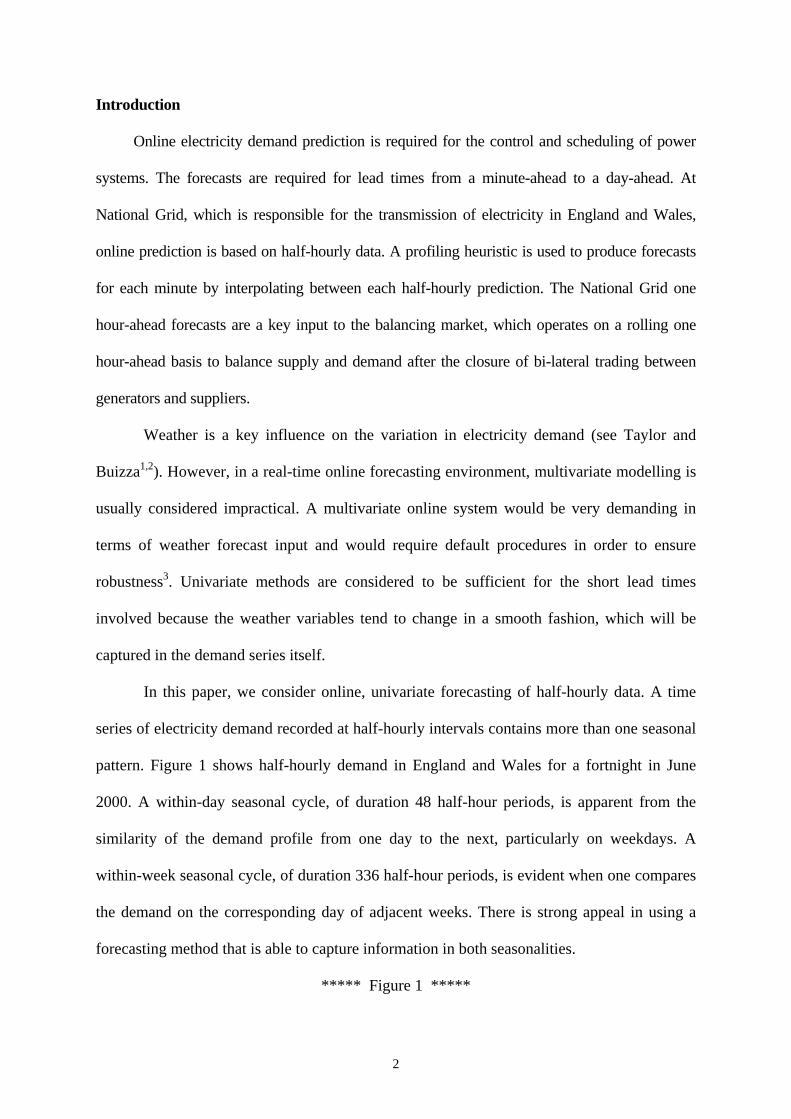
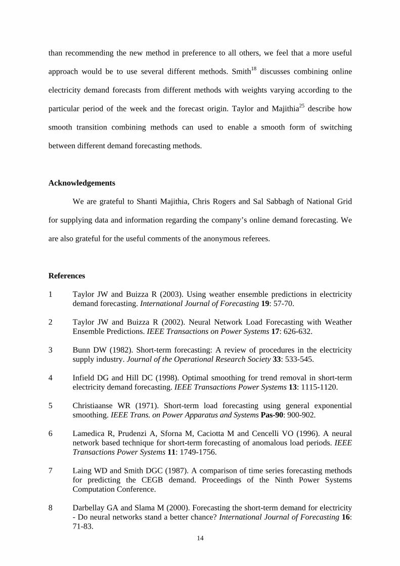
In this paper, we consider online, univariate forecasting of half-hourly data. A time

series of electricity demand recorded at half-hourly intervals contains more than one seasonal

pattern. Figure 1 shows half-hourly demand in England and Wales for a fortnight in June

2000. A within-day seasonal cycle, of duration 48 half-hour periods, is apparent from the

similarity of the demand profile from one day to the next, particularly on weekdays. A

within-week seasonal cycle, of duration 336 half-hour periods, is evident when one compares

the demand on the corresponding day of adjacent weeks. There is strong appeal in using a

forecasting method that is able to capture information in both seasonalities.

***** Figure 1 *****

3

Holt-Winters exponential smoothing is a popular approach to forecasting seasonal

time series. The robustness and accuracy of exponential smoothing methods has led to their

widespread use in applications where a large number of series necessitates an automated

procedure, such as inventory control. This suggests that Holt-Winters might be a reasonable

candidate for the automated application of online electricity demand forecasting. However,

the method is only able to accommodate one seasonal pattern. The multiplicative seasonal

ARIMA model has been extended in order to model the within-day and within-week

seasonalities in electricity demand. In this paper, we adapt the Holt-Winters method so that it

can accommodate two seasonalities. This involves the introduction of an additional seasonal

index and an extra smoothing equation for the new seasonal index.

In the next section, we describe how ARIMA models have been adapted for online

electricity demand forecasting, in order to capture multiple seasonalities in the demand series.

We then show how the Holt-Winters method can be adapted for series with more than one

seasonality. The section that follows presents an empirical forecast comparison of the new

formulation with the standard Holt-Winters method and with a multiplicative double seasonal

ARIMA model. In the final section, we provide a summary and conclusion.

Multiplicative Double Seasonal ARIMA Models

The literature on short-term load forecasting contains a variety of univariate methods

that could be implemented in an online prediction system. The range of different approaches

includes state space methods with the Kalman filter (e.g. Infield and Hill4), general

exponential smoothing (e.g. Christiaanse5), artificial neural networks (e.g. Lamedica et al.6),

spectral methods (e.g. Laing and Smith7) and seasonal ARIMA models (e.g. Laing and

Smith7; Darbellay and Slama8). The most noticeable development in demand forecasting over

the last decade has been the increasing interest shown by researchers and practitioners in

artificial neural networks (see Hippert et al. 9). Although there is obvious appeal to using this

modelling approach to find the non-linear relationship between demand and weather

variables, its appeal for univariate modelling is far less clear. The one short-term forecasting

method that has remained popular over the years, and appears in many papers as a benchmark

approach, is multiplicative seasonal ARIMA modelling.

The multiplicative seasonal ARIMA model, for a series, Xt, with just one seasonal pattern

can be written as

( ) ( ) ( ) ( ) ts

QqtDs

dsPp LLXLL εθφ Θ=∇∇Φ

where L is the lag operator, s is the number of periods in a seasonal cycle, ∇ is the difference

operator, (1-L), ∇s is the seasonal difference operator, (1-Ls), d and D are the orders of

differencing, εt is a white noise error term, and φp, ΦP, θq and ΘQ are polynomial functions of

orders p, P, q and Q, respectively. The model is often expressed as ARIMA(p,d,q)×(P,D,Q)s.

It is multiplicative in the sense that the polynomial functions of L and Ls are multiplied on

each side of the equation to give a rich function of the lag operator. Box et al. 10 (p 333)

comment that the model can be extended for the case of multiple seasonalities. The

multiplicative double seasonal ARIMA model can be written as

( ) ( ) ( ) ( ) ( ) ( ) ts

Qs

QqtDs

Ds

dsP

sPp LLLXLLL εθφ 2

2

1

1

2

2

1

1

2

2

1

1ΨΘ=∇∇∇ΩΦ (1)

where s1 and s2 are the number of periods in the different seasonal cycles, and and 2PΩ

2QΨ

are polynomial functions of orders P2 and Q2, respectively. This model can be expressed as

ARIMA . Applying the model to half-hourly electricity

demand, Laing and Smith

21),,(),,(),,( 222111 ss QDPQDPqdp ××

7 set s1=48 to model the within-day seasonal cycle of 48 half-hours,

and s2=336 to model the within-week cycle of 336 half-hours. The forecasts from ARIMA

models of this type are currently used at National Grid. In an application to hourly demand in

the Czech Republic, Darbellay and Slama8 set s1=24 to model the within-day seasonal cycle,

and s2=168 to model the within-week cycle.

4

The multiplicative seasonal ARIMA model can easily be extended to take care of

three or more seasonalities by the introduction of additional polynomial functions of the lag

operator and additional difference operators in expression (1). Therefore, the annual seasonal

pattern in electricity demand could also be modelled. However, it is usual to assume that it is

not significant in the context of lead times up to a day-ahead7.

In this section, we have shown how the multiplicative double seasonal ARIMA model

is a straightforward extension of the standard multiplicative seasonal model. Motivated by

this, and by the fact that exponential smoothing has been a competitive alternative to ARIMA

models with a variety of different types of data11, in the next section, we adapt the standard

Holt-Winters method for application to series with two seasonalities.

Double Seasonal Holt-Winters Exponential Smoothing

Standard Holt-Winters

The standard Holt-Winters method was introduced by Winters12 and is suitable for

series with one seasonal pattern. The multiplicative seasonality version of the method is

presented in expressions (2)-(5). It assumes an additive trend and estimates the local slope, Tt,

by smoothing successive differences, (St - St-1), of the local level, St. The local s-period

seasonal index, It, is estimated by smoothing the ratio of observed value, Xt, to local level, St.

Level )()1()( 11 −−− +−+= ttsttt TSIXS αα (2) Trend 11 )1()( −− −+−= tttt TSST γγ (3) Seasonality stttt ISXI −−+= )1()( δδ (4)

kstttt ITkSkX +−+= )()(ˆ (5)

where α, γ and δ are smoothing parameters, and is the k-step-ahead forecast. The

seasonality is multiplicative in the sense that the underlying level of the series is multiplied

by the seasonal index. Holt-Winters for additive seasonality is an alternative formulation,

which involves the addition of seasonal factors to the underlying trend. The multiplicative

version is appropriate if the magnitude of the seasonal variation increases with an increase in

)(ˆ kX t

5

the mean level of the series, while the additive version should be used if the seasonal effect

does not depend on the current mean level. The multiplicative version is much more widely

used and so for simplicity, in this paper, we provide only the multiplicative formulation.

It is worth noting that the use of the word “multiplicative” in the context of seasonal

ARIMA models is quite different to its use in Holt-Winters exponential smoothing. By

contrast with Holt-Winters for multiplicative seasonality, the seasonal effect for

multiplicative seasonal ARIMA models does not depend on the mean level of the series.

There is no equivalence between Holt-Winters for multiplicative seasonality and

multiplicative seasonal ARIMA models. This point is, perhaps, emphasised by the fact that,

although there is an ARIMA model for which Holt-Winters for additive seasonality is

optimal13, there is no ARIMA model for which Holt-Winters for multiplicative seasonality is

optimal14.

Double Seasonal Holt-Winters

Although standard Holt-Winters is widely used for forecasting seasonal time series,

the method is only able to accommodate one seasonal pattern. A formulation that can

accommodate more than one seasonal pattern has not been considered in the exponential

smoothing literature. This is evident from the recent taxonomies of Hyndman et al.15 and

Taylor16. The Holt-Winters method for double multiplicative seasonality is given in

expression (6)-(10). The method is suitable when there are two seasonal patterns in the time

series. The formulation involves separate seasonal indices, Dt and Wt, for the two

seasonalities. The local s1-period seasonal index, Dt, is estimated by smoothing the ratio of

observed value, Xt, to the product of the local level, St, and local s2-period seasonal index,

. Similarly, the local s2stW − 2-period seasonal index, Wt, is estimated by smoothing the ratio of

observed value, Xt, to the product of the local level, St, and local s1-period seasonal index,

. 1stD −

6

Level )()1())(( 1121 −−−− +−+= ttststtt TSWDXS αα (6)

Trend 11 )1()( −− −+−= tttt TSST γγ (7) Seasonality 1

12)1())(( ststttt DWSXD −− −+= δδ (8)

Seasonality 2 21

)1())(( ststttt WDSXW −− −+= ωω (9)

kstkstttt WDTkSkX +−+−+=21

)()(ˆ (10)

where α, γ, δ and ω are smoothing parameters. Applying the method to a series of half-hourly

demand, one would set s1=48 and s2=336, as in the multiplicative double seasonal ARIMA

model of Laing and Smith7. Dt and Wt would then represent the within-day and within-week

seasonalities, respectively. A double additive seasonality method can be developed in a

similar way from the standard Holt-Winters method for additive seasonality. The formulation

in expressions (6)-(10) can easily be extended for three or more seasonal patterns by

introducing an extra seasonal index and smoothing equation for each additional seasonality.

Empirical Comparison of Methods

We carried out empirical analysis in order to address two main issues. Firstly, we

wished to investigate whether the new double seasonal Holt-Winters method offers an

improvement on the standard Holt-Winters method in terms of forecast accuracy. Secondly,

we wanted to compare forecasting performance of the new formulation with a well-specified

multiplicative double seasonal ARIMA model.

The data used was 12 weeks of half-hourly electricity demand in England and Wales

from Monday 5 June 2000 to Sunday 27 August 2000. It is shown in Figure 2. We used the

first 8 weeks of data to estimate method parameters and the remaining 4 weeks to evaluate

post-sample forecasting performance. This amounts to 2,688 half-hourly observations for

estimation and 1,344 for evaluation. To simplify our comparison of methods, we chose a

period that did not contain any ‘special’ days, such as national holidays. Demand on these

days is so very unlike the rest of the year that online univariate methods are generally unable

to produce reasonable forecasts. In practice, interactive facilities tend to be used for special

7

days, which allow operator experience to supplement or override the system offline. If a

forecasting method is unable to tolerate gaps in the historical series, the special days can be

smoothed over, leaving the natural periodicities of the data intact7.

***** Figure 2 *****

Multiplicative Double Seasonal ARIMA

The process of model identification is impractical in an online demand forecasting

system, and so the model is chosen offline. We used the Box-Jenkins modelling methodology

to identify the most suitable ARIMA model based on the 2,688 observations in the estimation

sample. The autocorrelation function and partial autocorrelation function were used to select

the order of the model, which was then estimated by maximum likelihood. The residuals were

inspected for any remaining autocorrelation. Laing and Smith7 explain that, in the

multiplicative double seasonal ARIMA formulation in expression (1), polynomials of order

greater than two are rarely necessary when fitting a model to half-hourly data for England

and Wales. In view of this, we considered polynomials up to order two, but we also checked

the autocorrelation function of the residuals for any remaining higher order autocorrelation.

We compared the Schwartz Bayesian Criterion (SBC) for an extensive range of different

ARIMA models. We investigated differencing and a logarithmic transformation for demand

but found neither to improve the SBC. The model with lowest SBC and satisfactory residuals

was the following ARIMA(2,0,0)×(2,0,2)48×(2,0,2)336 model, which we shall refer to as the

Double Seasonal ARIMA model:

( )( )( )( )( )( t

t

LLL

XLLLLLL

ε67233696

67233696482

19.015.0116.01

625,2144.052.0131.032.0108.002.11

−−−=

−−−−−+−

)

8

Holt-Winters Exponential Smoothing

We produced forecasts using the following three Holt-Winters methods:

Holt-Winters for Within-Day Seasonality - This is standard Holt-Winters for multiplicative

seasonality, given in expressions (2)-(5), using only a 48-period seasonal cycle.

Holt-Winters for Within-Week Seasonality - This is standard Holt-Winters for multiplicative

seasonality, given in expressions (2)-(5), using only a 336-period seasonal cycle.

Double Seasonal Holt-Winters - This is the new Holt-Winters for double multiplicative

seasonality, given in expressions (6)-(10), using both a 48-period cycle for the within-day

seasonality and a 336-period seasonal cycle for the within-week seasonality.

Williams and Miller17 use simple averages of the first few data observations to

calculate initial smoothed values for the level, trend and seasonal components in the standard

Holt-Winters method. We implemented their procedure for Holt-Winters for Within-Day

Seasonality and Holt-Winters for Within-Week Seasonality. We adapted the procedure for

Double Seasonal Holt-Winters. The initial trend, T0, was chosen as the average of (1) 3361 of

the difference between the mean of the first 336 and second 336 observations, and (2) the

average of the first differences for the first 336 observations. The initial level, S0, was chosen

as the mean of the first 672 observations minus 336.5 times the initial trend. The initial values

for the within-day seasonal index, Dt, were set as the average of the ratios of actual

observation to 48-point centred moving average, taken from the corresponding half-hour

period in each of the first seven days of the time series. The initial values for the within-week

seasonal index, Wt, were set as the average of the ratios of actual observation to 336-point

centred moving average, taken from the corresponding half-hour period on the same day of

the week in each of the first two weeks of the demand series, divided by the corresponding

initial value of the smoothed within-day seasonal index, Dt.

We derived parameter values by the common procedure of minimising the sum of

squared 1-step-ahead forecast errors using a non-linear optimisation routine. The estimated

9

10

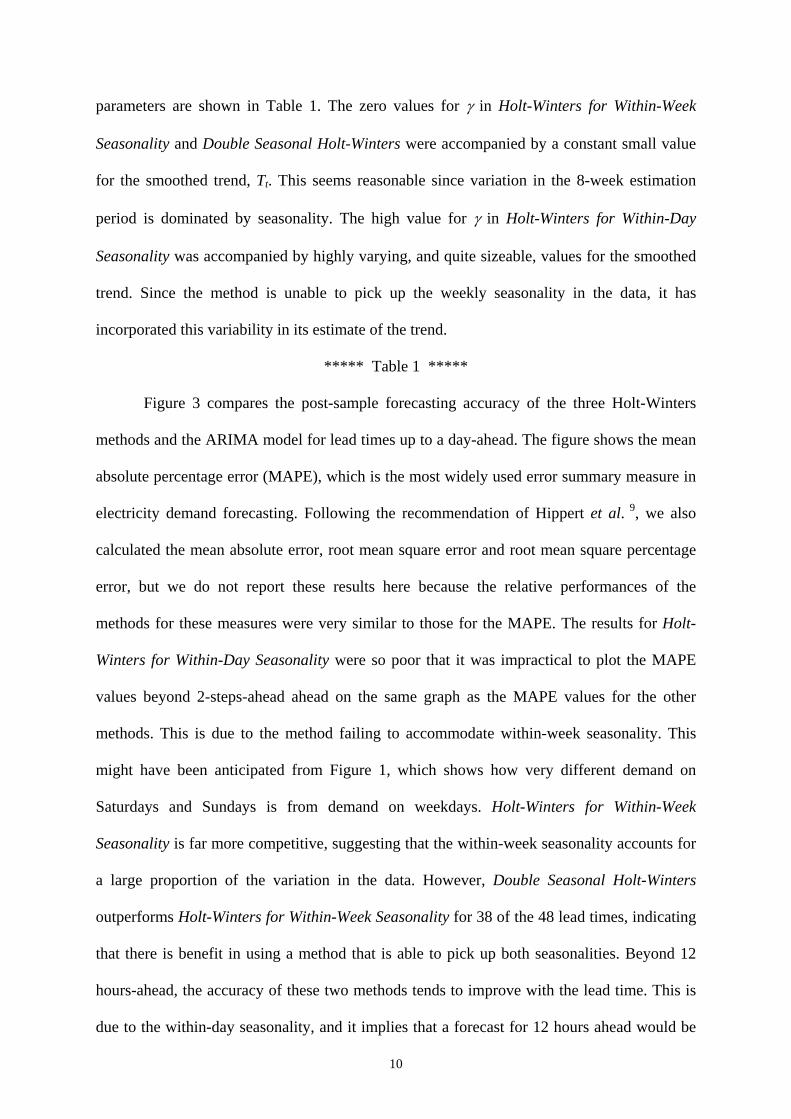
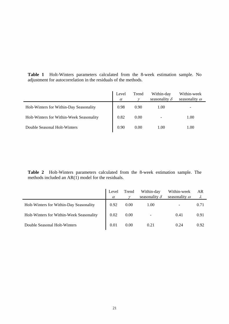
parameters are shown in Table 1. The zero values for γ in Holt-Winters for Within-Week

Seasonality and Double Seasonal Holt-Winters were accompanied by a constant small value

for the smoothed trend, Tt. This seems reasonable since variation in the 8-week estimation

period is dominated by seasonality. The high value for γ in Holt-Winters for Within-Day

Seasonality was accompanied by highly varying, and quite sizeable, values for the smoothed

trend. Since the method is unable to pick up the weekly seasonality in the data, it has

incorporated this variability in its estimate of the trend.

***** Table 1 *****

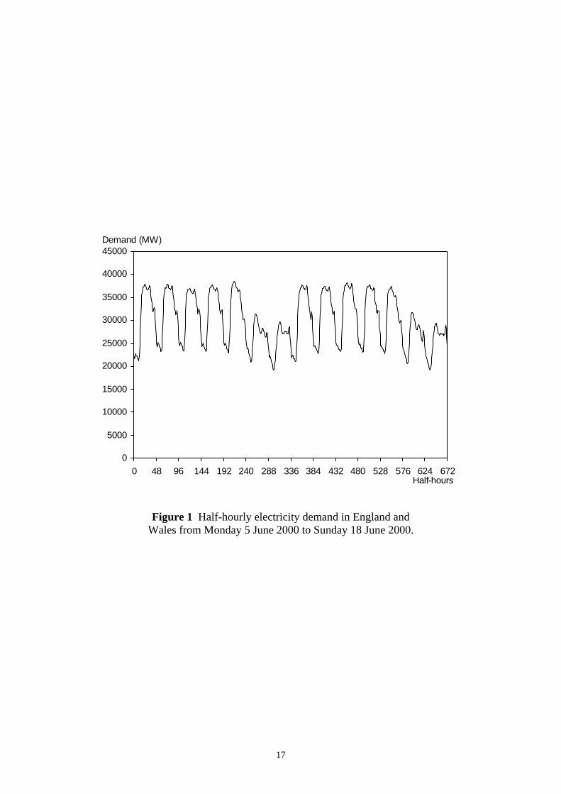
Figure 3 compares the post-sample forecasting accuracy of the three Holt-Winters

methods and the ARIMA model for lead times up to a day-ahead. The figure shows the mean

absolute percentage error (MAPE), which is the most widely used error summary measure in

electricity demand forecasting. Following the recommendation of Hippert et al. 9, we also

calculated the mean absolute error, root mean square error and root mean square percentage

error, but we do not report these results here because the relative performances of the

methods for these measures were very similar to those for the MAPE. The results for Holt-

Winters for Within-Day Seasonality were so poor that it was impractical to plot the MAPE

values beyond 2-steps-ahead ahead on the same graph as the MAPE values for the other

methods. This is due to the method failing to accommodate within-week seasonality. This

might have been anticipated from Figure 1, which shows how very different demand on

Saturdays and Sundays is from demand on weekdays. Holt-Winters for Within-Week

Seasonality is far more competitive, suggesting that the within-week seasonality accounts for

a large proportion of the variation in the data. However, Double Seasonal Holt-Winters

outperforms Holt-Winters for Within-Week Seasonality for 38 of the 48 lead times, indicating

that there is benefit in using a method that is able to pick up both seasonalities. Beyond 12

hours-ahead, the accuracy of these two methods tends to improve with the lead time. This is

due to the within-day seasonality, and it implies that a forecast for 12 hours ahead would be

11

better made from a forecast origin 12 hours prior to the current period. In his analysis of

online methods, Smith18 also concludes that the choice of forecast origin should depend on

the forecast horizon. Comparing the two double seasonal methods, we see that Double

Seasonal ARIMA outperforms Double Seasonal Holt-Winters for all but the last 5 lead times.

***** Figure 3 *****

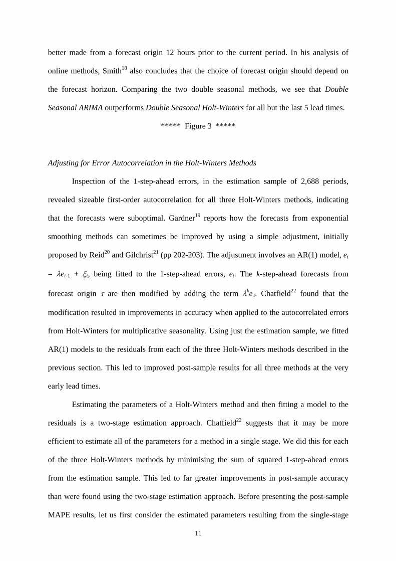
Adjusting for Error Autocorrelation in the Holt-Winters Methods

Inspection of the 1-step-ahead errors, in the estimation sample of 2,688 periods,

revealed sizeable first-order autocorrelation for all three Holt-Winters methods, indicating

that the forecasts were suboptimal. Gardner19 reports how the forecasts from exponential

smoothing methods can sometimes be improved by using a simple adjustment, initially

proposed by Reid20 and Gilchrist21 (pp 202-203). The adjustment involves an AR(1) model, et

= λet-1 + ξt, being fitted to the 1-step-ahead errors, et. The k-step-ahead forecasts from

forecast origin τ are then modified by adding the term λkeτ. Chatfield22 found that the

modification resulted in improvements in accuracy when applied to the autocorrelated errors

from Holt-Winters for multiplicative seasonality. Using just the estimation sample, we fitted

AR(1) models to the residuals from each of the three Holt-Winters methods described in the

previous section. This led to improved post-sample results for all three methods at the very

early lead times.

Estimating the parameters of a Holt-Winters method and then fitting a model to the

residuals is a two-stage estimation approach. Chatfield22 suggests that it may be more

efficient to estimate all of the parameters for a method in a single stage. We did this for each

of the three Holt-Winters methods by minimising the sum of squared 1-step-ahead errors

from the estimation sample. This led to far greater improvements in post-sample accuracy

than were found using the two-stage estimation approach. Before presenting the post-sample

MAPE results, let us first consider the estimated parameters resulting from the single-stage

12

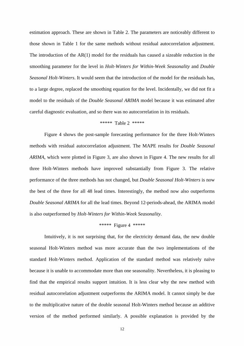
estimation approach. These are shown in Table 2. The parameters are noticeably different to

those shown in Table 1 for the same methods without residual autocorrelation adjustment.

The introduction of the AR(1) model for the residuals has caused a sizeable reduction in the

smoothing parameter for the level in Holt-Winters for Within-Week Seasonality and Double

Seasonal Holt-Winters. It would seem that the introduction of the model for the residuals has,

to a large degree, replaced the smoothing equation for the level. Incidentally, we did not fit a

model to the residuals of the Double Seasonal ARIMA model because it was estimated after

careful diagnostic evaluation, and so there was no autocorrelation in its residuals.

***** Table 2 *****

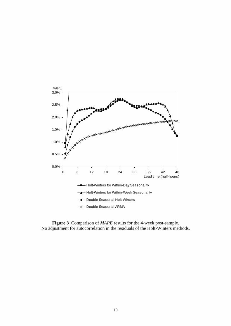
Figure 4 shows the post-sample forecasting performance for the three Holt-Winters

methods with residual autocorrelation adjustment. The MAPE results for Double Seasonal

ARIMA, which were plotted in Figure 3, are also shown in Figure 4. The new results for all

three Holt-Winters methods have improved substantially from Figure 3. The relative

performance of the three methods has not changed, but Double Seasonal Holt-Winters is now

the best of the three for all 48 lead times. Interestingly, the method now also outperforms

Double Seasonal ARIMA for all the lead times. Beyond 12-periods-ahead, the ARIMA model

is also outperformed by Holt-Winters for Within-Week Seasonality.

***** Figure 4 *****

Intuitively, it is not surprising that, for the electricity demand data, the new double

seasonal Holt-Winters method was more accurate than the two implementations of the

standard Holt-Winters method. Application of the standard method was relatively naïve

because it is unable to accommodate more than one seasonality. Nevertheless, it is pleasing to

find that the empirical results support intuition. It is less clear why the new method with

residual autocorrelation adjustment outperforms the ARIMA model. It cannot simply be due

to the multiplicative nature of the double seasonal Holt-Winters method because an additive

version of the method performed similarly. A possible explanation is provided by the

13

comments of Chatfield23 and Chatfield and Yar24 in their consideration of the choice between

ARIMA modelling and exponential smoothing. They explain that ARIMA modelling is worth

considering if the series is dominated by short-term correlation but not when it is dominated

by trend and seasonal variation. Since electricity demand, recorded at half-hourly or hourly

intervals, is dominated by seasonal variation, it follows that Holt-Winters formulations

should perform well in comparison with ARIMA models.

Summary and Conclusions

Online short-term electricity demand forecasting requires a robust, univariate

procedure. Inspection of a time series of half-hourly demand reveals a within-day seasonality

and a within-week seasonality. A popular approach is to use a multiplicative double seasonal

ARIMA model. The robustness of exponential smoothing methods suggests that Holt-

Winters would be a reasonable candidate for online short-term demand forecasting. However,

the method is only able to accommodate one seasonal pattern. In this paper, we have shown

how the method can be adapted for time series with two seasonalities. This involves the

introduction of an additional seasonal index and an extra smoothing equation for this new

seasonal index.

Using a series of half-hourly electricity demand, the new formulation outperformed

standard Holt-Winters for forecast lead times from a half-hour-ahead to a day-ahead. The

Holt-Winters methods were improved by the inclusion of an AR(1) model for the residuals.

The best results were achieved by estimating the AR(1) model parameter in the same

estimation procedure as the exponential smoothing parameters. The resulting forecasts for the

new double seasonal Holt-Winters method outperformed those from standard Holt-Winters

and also those from a well-specified multiplicative double seasonal ARIMA model. We,

therefore, conclude that there is strong potential for the use of the new double seasonal Holt-

Winters formulation in online short-term electricity demand forecasting. However, rather

14

than recommending the new method in preference to all others, we feel that a more useful

approach would be to use several different methods. Smith18 discusses combining online

electricity demand forecasts from different methods with weights varying according to the

particular period of the week and the forecast origin. Taylor and Majithia25 describe how

smooth transition combining methods can used to enable a smooth form of switching

between different demand forecasting methods.

Acknowledgements

We are grateful to Shanti Majithia, Chris Rogers and Sal Sabbagh of National Grid

for supplying data and information regarding the company’s online demand forecasting. We

are also grateful for the useful comments of the anonymous referees.

References

1 Taylor JW and Buizza R (2003). Using weather ensemble predictions in electricity demand forecasting. International Journal of Forecasting 19: 57-70.

2 Taylor JW and Buizza R (2002). Neural Network Load Forecasting with Weather

Ensemble Predictions. IEEE Transactions on Power Systems 17: 626-632. 3 Bunn DW (1982). Short-term forecasting: A review of procedures in the electricity

supply industry. Journal of the Operational Research Society 33: 533-545. 4 Infield DG and Hill DC (1998). Optimal smoothing for trend removal in short-term

electricity demand forecasting. IEEE Transactions Power Systems 13: 1115-1120. 5 Christiaanse WR (1971). Short-term load forecasting using general exponential

smoothing. IEEE Trans. on Power Apparatus and Systems Pas-90: 900-902. 6 Lamedica R, Prudenzi A, Sforna M, Caciotta M and Cencelli VO (1996). A neural

network based technique for short-term forecasting of anomalous load periods. IEEE Transactions Power Systems 11: 1749-1756.

7 Laing WD and Smith DGC (1987). A comparison of time series forecasting methods

for predicting the CEGB demand. Proceedings of the Ninth Power Systems Computation Conference.

8 Darbellay GA and Slama M (2000). Forecasting the short-term demand for electricity

- Do neural networks stand a better chance? International Journal of Forecasting 16: 71-83.

15

9 Hippert HS, Pedreira CE and Souza RC (2001). Neural networks for short-term load forecasting: A review and evaluation. IEEE Transactions on Power Systems 16: 44-55.

10 Box GEP, Jenkins GM and Reinsel GC (1994). Time Series Analysis: Forecasting

and Control, third edition. Englewod Cliffs, Prentice Hall: New Jersey, p 333. 11 Makridakis S, Chatfield C, Hibon M, Lawrence M, Mills T, Ord K and Simmons LF

(1993). The M2-Competition: A real-time judgementally based forecasting study. International Journal of Forecasting 9: 5-22.

12 Winters PR (1960). Forecasting sales by exponentially weighted moving averages.

Management Science 6: 324-342. 13 McKenzie E (1976). A comparison of some standard seasonal forecasting systems.

The Statistician 25: 3-14. 14 Abraham B and Ledolter J (1986). Forecast functions implied by autoregressive

integrated moving average and other related forecast procedures. International Statistical Review 54: 51-66.

15 Hyndman RJ, Koehler AB, Snyder RD and Grose S (2002). A state space framework

for automatic forecasting using exponential smoothing methods. International Journal of Forecasting 18: 439-454.

16 Taylor JW (2003). Damped multiplicative trend exponential smoothing. International

Journal of Forecasting forthcoming. 17 Williams DW and Miller D (1999). Level-adjusted exponential smoothing for modeling

planned discontinuities. International Journal of Forecasting 15: 273-289. 18 Smith DGC (1989). Combination of forecasts in electricity demand prediction.

Journal of Forecasting 8: 349-356. 19 Gardner ES Jr. (1985). Exponential smoothing: The state of the art. Journal of

Forecasting 4: 1-28. 20 Reid DJ (1975). A review of short-term projection techniques. In: Practical Aspects of

Forecasting, Gordon HA (ed.). Operational Research Society, London, pp 8-25. 21 Gilchrist W (1976). Statistical Forecasting. Wiley: Chichester. 22 Chatfield C (1978). The Holt-Winters forecasting procedure. Applied Statistics 27:

264-279. 23 Chatfield C (1985). Comments on ‘Exponential smoothing: The state of the art’ by

Gardner ES Jr. Journal of Forecasting 4: 30. 24 Chatfield C and Yar M (1988). Holt-Winters forecasting: Some practical issues. The

Statistician 37: 129-140.

16

25 Taylor JW and Majithia S (2000). Using combined forecasts with changing weights for electricity demand profiling. Journal of the Operational Research Society 51: 72-82.

0

5000

10000

15000

20000

25000

30000

35000

40000

45000

0 48 96 144 192 240 288 336 384 432 480 528 576 624 672Half-hours

Demand (MW)

Figure 1 Half-hourly electricity demand in England and Wales from Monday 5 June 2000 to Sunday 18 June 2000.

17

Demand (MW)

0

5000

10000

15000

20000

25000

30000

35000

40000

45000

0 336 672 1008 1344 1680 2016 2352 2688 3024 3360 3696 4032Half-hours

Figure 2 Half-hourly electricity demand in England and Wales from Monday 5 June 2000 to Sunday 27 August 2000.

18

0.0%

0.5%

1.0%

1.5%

2.0%

2.5%

3.0%

0 6 12 18 24 30 36 42 48Lead time (half-hours)

MAPE

Holt-Winters for Within-Day Seasonality

Holt-Winters for Within-Week Seasonality

Double Seasonal Holt-Winters

Double Seasonal ARMA

Figure 3 Comparison of MAPE results for the 4-week post-sample.

No adjustment for autocorrelation in the residuals of the Holt-Winters methods.

19

0.0%

0.5%

1.0%

1.5%

2.0%

2.5%

3.0%

0 6 12 18 24 30 36 42 48Lead time (half-hours)

MAPE

Holt-Winters for Within-Day Seasonality with AR(1) Adjustment

Holt-Winters for Within-Week Seasonality with AR(1) Adjustment

Double Seasonal Holt-Winters with AR(1) Adjustment

Double Seasonal ARMA

Figure 4 Comparison of MAPE results for the 4-week post-sample period. The Holt-Winters methods included an AR(1) model for the residuals.

20

21

Table 1 Holt-Winters parameters calculated from the 8-week estimation sample. No adjustment for autocorrelation in the residuals of the methods.

Level α

Trend γ

Within-day seasonality δ

Within-week seasonality ω

Holt-Winters for Within-Day Seasonality 0.98 0.90 1.00 -

Holt-Winters for Within-Week Seasonality 0.82 0.00 - 1.00

Double Seasonal Holt-Winters 0.90 0.00 1.00 1.00

Table 2 Holt-Winters parameters calculated from the 8-week estimation sample. The methods included an AR(1) model for the residuals.

Level α

Trend γ

Within-day seasonality δ

Within-week seasonality ω

AR λ

Holt-Winters for Within-Day Seasonality 0.92 0.00 1.00 - 0.71

Holt-Winters for Within-Week Seasonality 0.02 0.00 - 0.41 0.91

Double Seasonal Holt-Winters 0.01 0.00 0.21 0.24 0.92