Shivkumar Kalyanaraman 1 Routing I: Basic Ideas Shivkumar Kalyanaraman Rensselaer Polytechnic Institute [email protected] Based in part upon slides

Shivkumar Kalyanaraman

1

Routing I: Basic Ideas

Shivkumar KalyanaramanRensselaer Polytechnic Institute

[email protected]

Based in part upon slides of Prof. Raj Jain (OSU), S. Keshav (Cornell), J. Kurose (U Mass), Noel Chiappa (MIT)


2

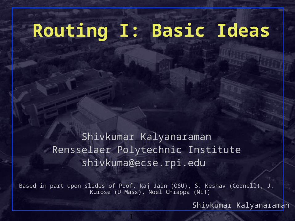
Routing vs Forwarding Forwarding table vs Forwarding in simple topologies Routers vs Bridges: review Routing Problem Telephony vs Internet Routing Source-based vs Fully distributed Routing Distance vector vs Link state routing Addressing and Routing: Scalability Refs: Chap 8, 11, 14, 16 in Comer textbook Books: “Routing in Internet” by Huitema, “Interconnections” by Perlman Reading: Notes for Protocol Design, E2e Principle, IP and Routing: In PDF Reading: Routing 101: Notes on Routing: In PDF | In MS Word Reading: Khanna and Zinky, The revised ARPANET routing metric Reference: Garcia-Luna-Aceves: "Loop-free Routing Using Diffusing Computations" : Reading: Alaettinoglu, Jacobson, Yu: "Towards Milli-Second IGP Convergence"

Overview


3

Routing vs Forwarding Forwarding table vs Forwarding in simple topologies

Routers vs Bridges: review Routing Problem Telephony vs Internet Routing Source-based vs Fully distributed Routing Distance vector vs Link state routing Addressing and Routing: Scalability

Where are we?


4

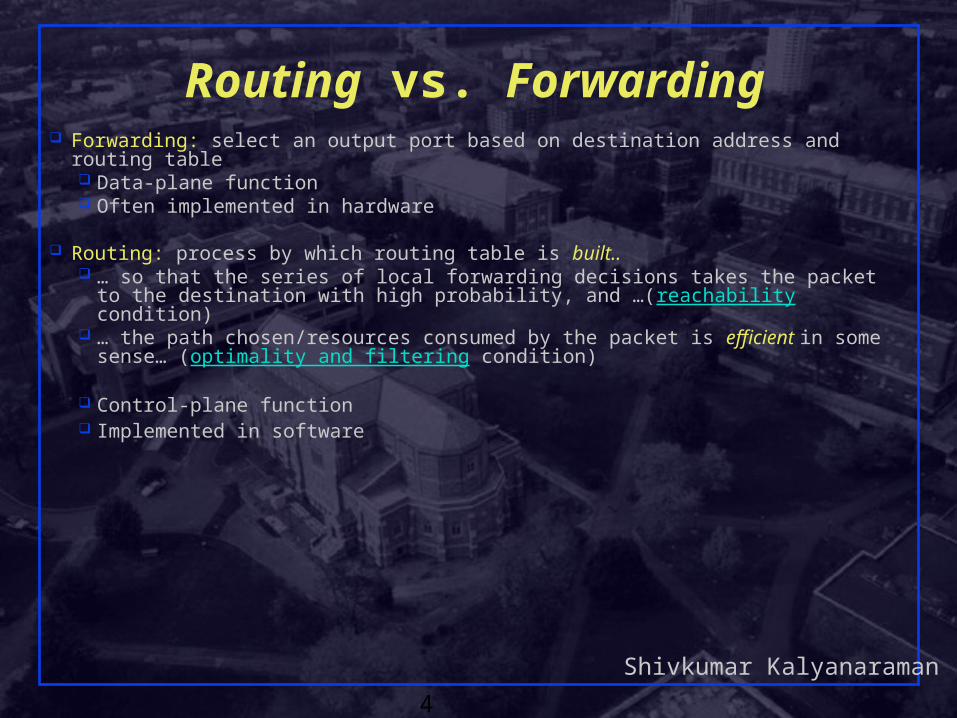
Routing vs. Forwarding Forwarding: select an output port based on destination address and routing table

Data-plane function Often implemented in hardware

Routing: process by which routing table is built.. … so that the series of local forwarding decisions takes the packet to the

destination with high probability, and …(reachability condition) … the path chosen/resources consumed by the packet is efficient in some

sense… (optimality and filtering condition)

Control-plane function Implemented in software


5

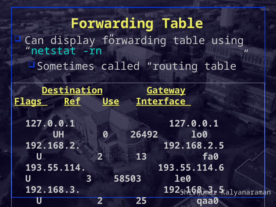
Forwarding Table Can display forwarding table using “netstat -rn”

Sometimes called “routing table”

Destination Gateway Flags Ref Use Interface 127.0.0.1 127.0.0.1 UH 0 26492 lo0 192.168.2. 192.168.2.5 U 2 13 fa0 193.55.114. 193.55.114.6 U 3 58503 le0 192.168.3. 192.168.3.5 U 2 25 qaa0 224.0.0.0 193.55.114.6 U 3 0 le0 default 193.55.114.129 UG 0 143454


6

Forwarding Table Structure Fields: destination, gateway, flags, ... Destination: can be a host address or a network

address. If the ‘H’ flag is set, it is the host address. Gateway: router/next hop IP address. The ‘G’ flag says

whether the destination is directly or indirectly connected. U flag: Is route up ? G flag: router (indirect vs direct) H flag: host (dest field: host or n/w address?)

Key question: Why did we need this forwarding table in the first

place ?


7

Routing in Simple Topologies

. . .

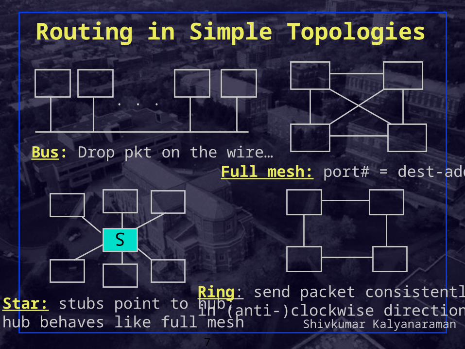
Full mesh: port# = dest-addrBus: Drop pkt on the wire…

Star: stubs point to hub;hub behaves like full mesh

S

Ring: send packet consistently in (anti-)clockwise direction


8

Routing vs Forwarding Forwarding table vs Forwarding in simple topologies

Routers vs Bridges: review

Routing Problem Telephony vs Internet Routing Source-based vs Fully distributed Routing Distance vector vs Link state routing Addressing and Routing: Scalability

Where are we?


9

Recall… Layer 1 & 2 Layer 1: Hubs do not have “forwarding tables” – they simply broadcast

signals at Layer 1. No filtering. Layer 2:

Forwarding tables not required for simple topologies (previous slide): simple forwarding rules suffice

The next-hop could be functionally related to destination address (i.e. it can be computed without a table explicitly listing the mapping).

This places too many restrictions on topology and the assignment of addresses vis-à-vis ports at intermediate nodes.

Forwarding tables could be statically (manually) configured once or from time-to-time.

Does not accommodate dynamism in topology


10

Recall… Layer 2 Even reasonable sized LANs cannot tolerate above

restrictions Bridges therefore have “L2 forwarding tables,” and use

dynamic learning algorithms to build it locally. Even this allows LANs to scale, by limiting broadcasts

and collisions to collision domains, and using bridges to interconnect collision domains.

The learning algorithm is purely local, opportunistic and expects no addressing structure.

Hence, bridges often may not have a forwarding entry for a destination address (I.e. incomplete)

In this case they resort to flooding – which may lead to duplicates of packets seen on the wire.

Bridges coordinate “globally” to build a spanning tree so that flooding doesn’t go out of control.


11

Recall …: Layer 3 Routers have “L3 forwarding tables,” and use a distributed

protocol to coordinate with other routers to learn and condense a global view of the network in a consistent and complete manner.

Routers NEVER broadcast or flood if they don’t have a route – they “pass the buck” to another router. The good filtering in routers (I.e. restricting broadcast and

flooding activity to be within broadcast domains) allows them to interconnect broadcast domains,

Routers communicate with other routers, typically neighbors to collect an abstracted view of the network. In the form of distance vector or link state. Routers use algorithms like Dijkstra, Bellman-Ford to

compute paths with such abstracted views.


12

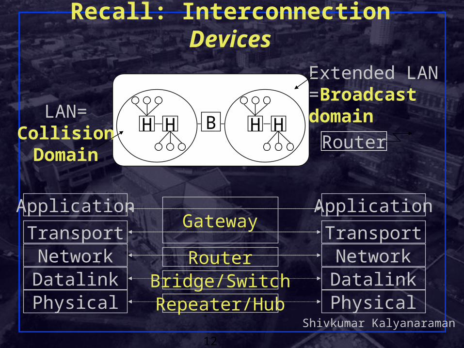
Recall: Interconnection Devices

H H B H HRouter

Extended LAN=Broadcast domainLAN=

CollisionDomain

NetworkDatalinkPhysical

TransportRouter

Bridge/SwitchRepeater/Hub

GatewayApplication

NetworkDatalinkPhysical

Transport

Application


13

Summary so far If topology is simple and static, routing is simple and may

not even require a forwarding table

If topology is dynamic, but filtering requirements are weak (I.e. network need not scale), then a local heuristic setup of forwarding table (bridging approach) suffices.

Further, if a) filtering requirements are strict, b) optimal/efficient routing is desired, and c) we want small forwarding tables and bounded control traffic, then … some kind of global communication, and smart distributed

algorithms are needed to condense global state in a consistent, but yet complete way …


14

What’s up in advanced routing? Routers are efficient in the collection of the abstracted

view (control-plane filtering) Routers accommodate a variety of topologies, and sub-

networks in an efficient manner Routers are organized in hierarchies to achieve

scalability; and into autonomous systems to achieve complex policy-control over routing.

Routers then condense paths into next hops, either: depending upon other routers in a path to compute

next-hops in a consistent manner (fully distributed), or using a signaling protocol to enforce consistency.

Advanced routing algorithms support “QoS routing” and “traffic engineering” goals like multi-path routing, source-based or distributed traffic splitting, fast re-route, path protection etc.


15

Routing vs Forwarding Forwarding table vs Forwarding in simple topologies Routers vs Bridges: review

Routing Problem

Telephony vs Internet Routing Source-based vs Fully distributed Routing Distance vector vs Link state routing Addressing and Routing: Scalability

Where are we?


16

Routing problem

Collect, process, and condense global state into local forwarding information

Global stateinherently largedynamichard to collect

Hard issues: consistency, completeness, scalabilityImpact of resource needs of sessions


17

Consistency Defn: A series of independent local forwarding decisions must

lead to connectivity between any desired (source, destination) pair in the network.

If the states are inconsistent, the network is said not to have “converged” to steady state (I.e. is in a transient state) Inconsistency leads to loops, wandering packets etc In general a part of the routing information may be

consistent while the rest may be inconsistent. Large networks => inconsistency is a scalability issue.

Consistency can be achieved in two ways: Fully distributed approach: a consistency criterion or

invariant across the states of adjacent nodes Signaled approach: the signaling protocol sets up local

forwarding information along the path.


18

Completeness Defn: The network as a whole and every node has

sufficient information to be able to compute all paths. In general, with more complete information available

locally, routing algorithms tend to converge faster, because the chances of inconsistency reduce.

But this means that more distributed state must be collected at each node and processed.

The demand for more completeness also limits the scalability of the algorithm.

Since both consistency and completeness pose scalability problems, large networks have to be structured hierarchically and abstract entire networks as a single node.


19

Design Choices … Centralized vs. distributed routing

Centralized is simpler, but prone to failure and congestion Centralized preferred in traffic engineering scenarios

where complex optimization problems need to be solved and where routes chosen are long-lived

Source-based (explicit) vs. hop-by-hop (fully distributed) Will the source-based route be signaled to fix the path and

to minimize packet header information? Eg: ATM, Frame-relay etc

Or will the route be condensed and placed in each header? Eg: IP routing option

Intermediate: loose source route


20

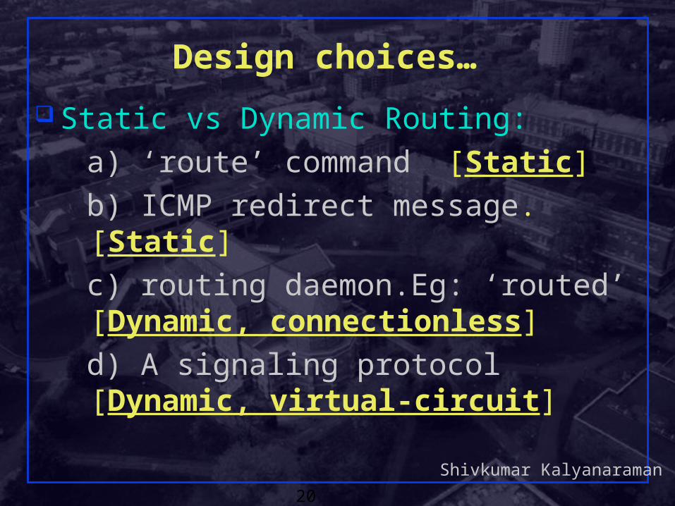
Design choices…

Static vs Dynamic Routing:

a) ‘route’ command [Static]

b) ICMP redirect message.[Static]

c) routing daemon.Eg: ‘routed’ [Dynamic, connectionless]

d) A signaling protocol [Dynamic, virtual-circuit]


21

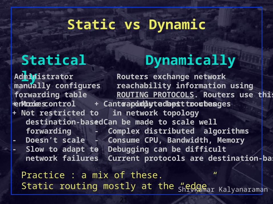
Static vs Dynamic

Statically DynamicallyRouters exchange network reachability information using ROUTING PROTOCOLS. Routers use this to compute best routes

Administrator manually configuresforwarding table entries

Practice : a mix of these.Static routing mostly at the “edge”

+ More control+ Not restricted to destination-based forwarding - Doesn’t scale- Slow to adapt to network failures

+ Can rapidly adapt to changes in network topology+ Can be made to scale well- Complex distributed algorithms- Consume CPU, Bandwidth, Memory- Debugging can be difficult- Current protocols are destination-based


22

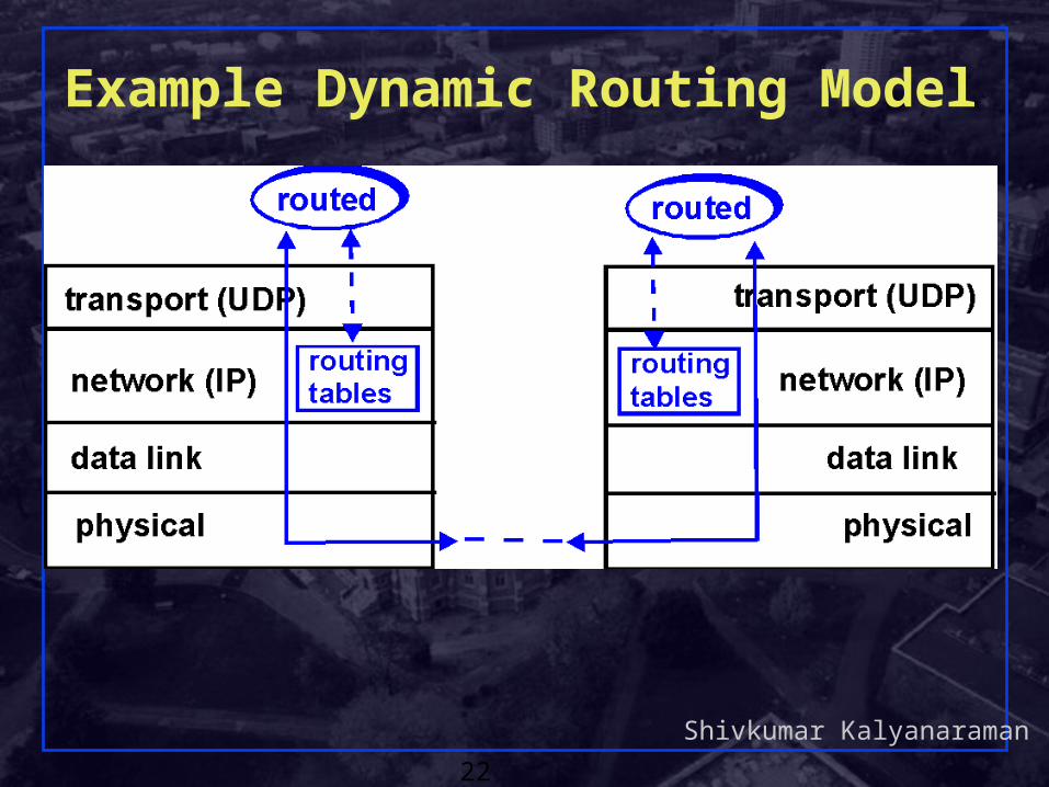
Example Dynamic Routing Model


23

Routing vs Forwarding Forwarding table vs Forwarding in simple topologies Routers vs Bridges: review Routing Problem

Telephony vs Internet Routing Source-based vs Fully distributed Routing

Distance vector vs Link state routing Addressing and Routing: Scalability

Where are we?


24

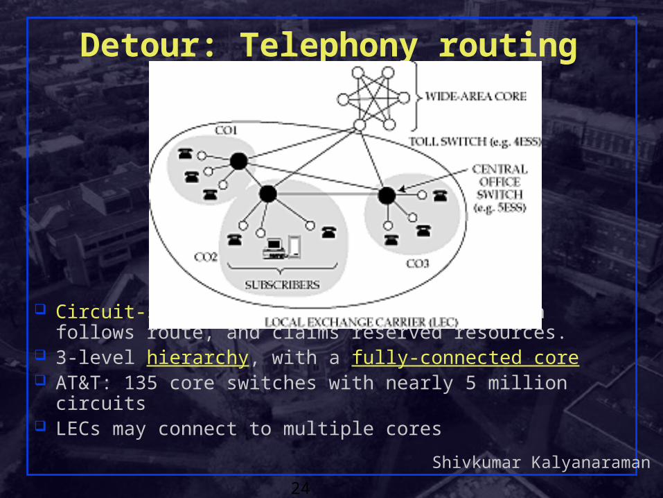
Detour: Telephony routing

Circuit-setup is what is routed. Voice then follows route, and claims reserved resources.

3-level hierarchy, with a fully-connected core AT&T: 135 core switches with nearly 5 million circuits LECs may connect to multiple cores


25

Telephony Routing algorithm

If endpoints are within same CO, directly connect If call is between COs in same LEC, use one-hop path

between COs Otherwise send call to one of the cores Only major decision is at toll switch

one-hop or two-hop path to the destination toll switch.

Essence of telephony routing problem:

which two-hop path to use if one-hop path is full

(almost a static routing problem… )


26

Features of telephone routing Resource reservation aspects:

Resource reservation is coupled with path reservationConnections need resources (same 64kbps)Signaling to reserve resources and the path

Stable loadNetwork built for voice only.Can predict pairwise load throughout the dayCan choose optimal routes in advance

Technology and economic aspects: Extremely reliable switches

Why? End-systems (phones) dumb because computation was non-existent in early 1900s.

Downtime is less than a few minutes per year => topology does not change dynamically


27

Features of telephone routingSource can learn topology and compute routeCan assume that a chosen route is available as the signaling

proceeds through the networkComponent reliability drove system reliability and hence

acceptance of service by customers Simplified topology:

Very highly connected networkHierarchy + full mesh at each level: simple routingHigh cost to achieve this degree of connectivity

Organizational aspects: Single organization controls entire core Afford the scale economics to build expensive network Collect global statistics and implement global changes

=> Source-based, signaled, simple alternate-path routing


28

Internet Routing Drivers Technology and economic aspects:

Internet built out of cheap, unreliable components as an overlay on top of leased telephone infrastructure for WAN transport.

Cheaper components => fail more often => topology changes often => needs dynamic routing

Components (including end-systems) had computation capabilities.

Distributed algorithms can be implemented Cheap overlaid inter-networks => several entities could

afford to leverage their existing (heterogeneous) LANs and leased lines to build inter-networks.

Led to multiple administrative “clouds” which needed to inter-connect for global communication.


29

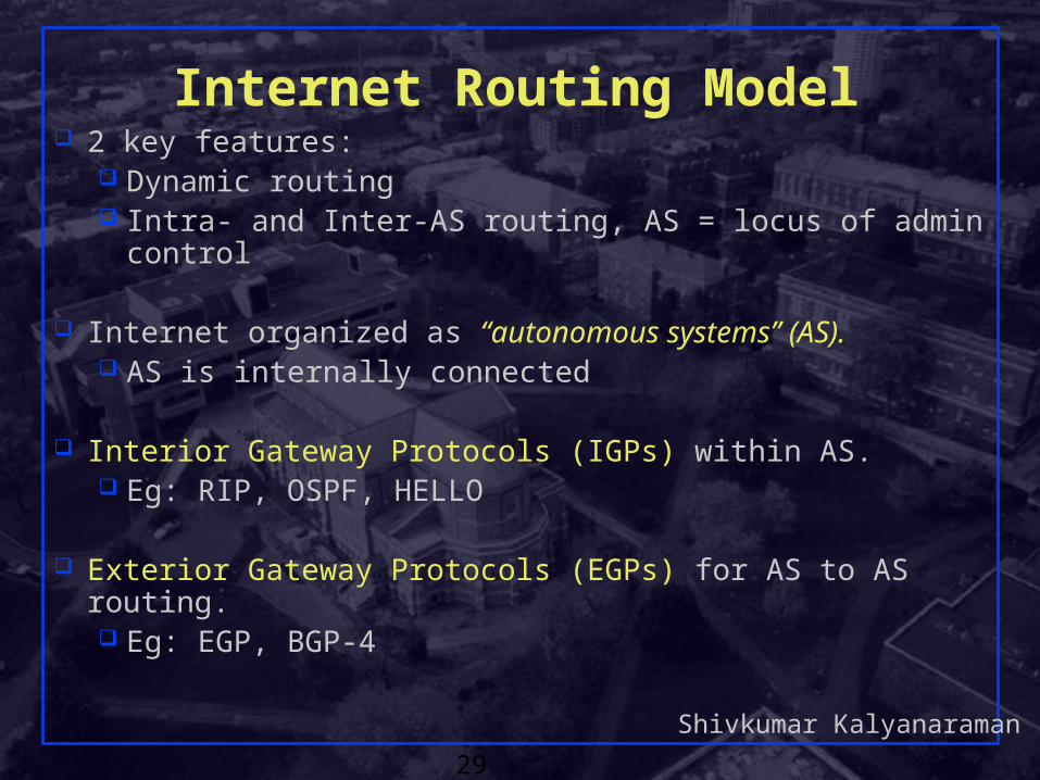
Internet Routing Model 2 key features:

Dynamic routing Intra- and Inter-AS routing, AS = locus of admin control

Internet organized as “autonomous systems” (AS). AS is internally connected

Interior Gateway Protocols (IGPs) within AS. Eg: RIP, OSPF, HELLO

Exterior Gateway Protocols (EGPs) for AS to AS routing. Eg: EGP, BGP-4


30

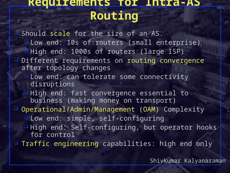
Requirements for Intra-AS Routing Should scale for the size of an AS.

Low end: 10s of routers (small enterprise) High end: 1000s of routers (large ISP)

Different requirements on routing convergence after topology changes Low end: can tolerate some connectivity disruptions High end: fast convergence essential to business

(making money on transport) Operational/Admin/Management (OAM) Complexity

Low end: simple, self-configuring High end: Self-configuring, but operator hooks for

control Traffic engineering capabilities: high end only


31

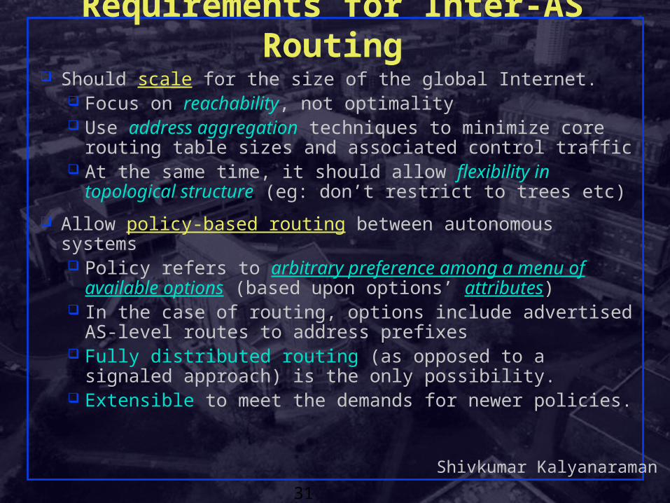
Requirements for Inter-AS Routing Should scale for the size of the global Internet.

Focus on reachability, not optimality Use address aggregation techniques to minimize core

routing table sizes and associated control traffic At the same time, it should allow flexibility in topological

structure (eg: don’t restrict to trees etc)

Allow policy-based routing between autonomous systems Policy refers to arbitrary preference among a menu of

available options (based upon options’ attributes) In the case of routing, options include advertised AS-level

routes to address prefixes Fully distributed routing (as opposed to a signaled approach)

is the only possibility. Extensible to meet the demands for newer policies.


32

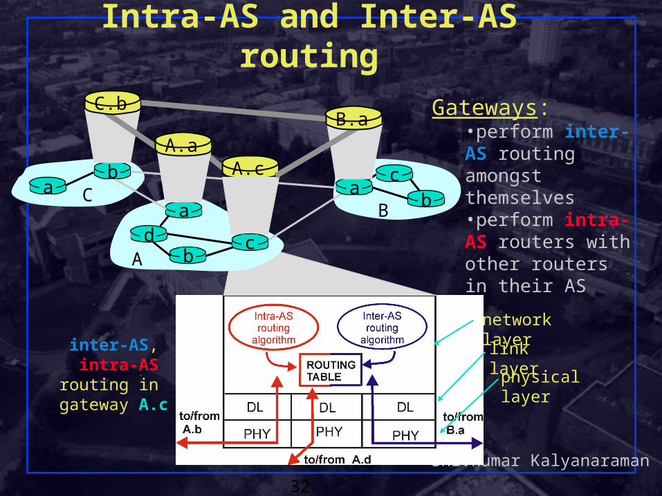
Intra-AS and Inter-AS routing

inter-AS, intra-AS routing in

gateway A.c

network layer

link layer

physical layer

a

b

b

aaC

A

Bd

Gateways:•perform inter-AS routing amongst themselves•perform intra-AS routers with other routers in their AS

A.cA.a

C.bB.a

cb

c


33

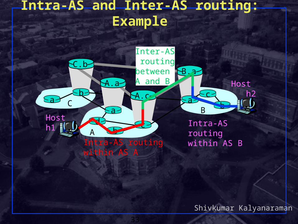
Intra-AS and Inter-AS routing: Example

Host h2

a

b

b

aaC

A

Bd c

A.a

A.c

C.bB.a

cb

Hosth1

Intra-AS routingwithin AS A

Inter-AS routingbetween A and B

Intra-AS routingwithin AS B


34

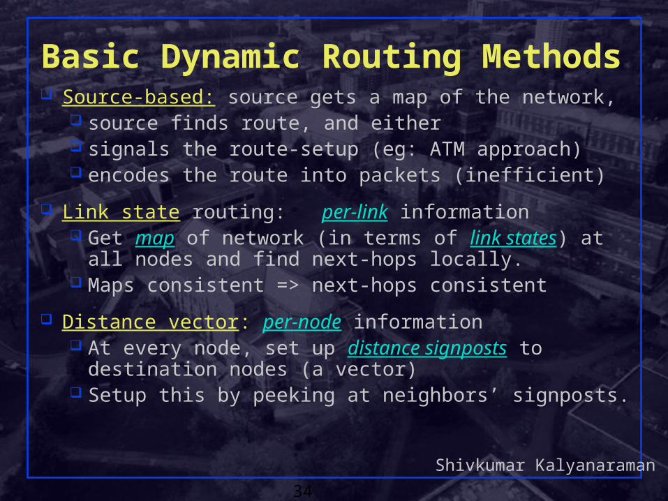
Basic Dynamic Routing Methods Source-based: source gets a map of the network,

source finds route, and either signals the route-setup (eg: ATM approach) encodes the route into packets (inefficient)

Link state routing: per-link information Get map of network (in terms of link states) at all

nodes and find next-hops locally. Maps consistent => next-hops consistent

Distance vector: per-node information At every node, set up distance signposts to destination

nodes (a vector) Setup this by peeking at neighbors’ signposts.


35

Routing vs Forwarding Forwarding table vs Forwarding in simple topologies Routers vs Bridges: review Routing Problem Telephony vs Internet Routing Source-based vs Fully distributed Routing

Distance vector vs Link state routing Bellman Ford and Dijkstra Algorithms

Addressing and Routing: Scalability

Where are we?


36

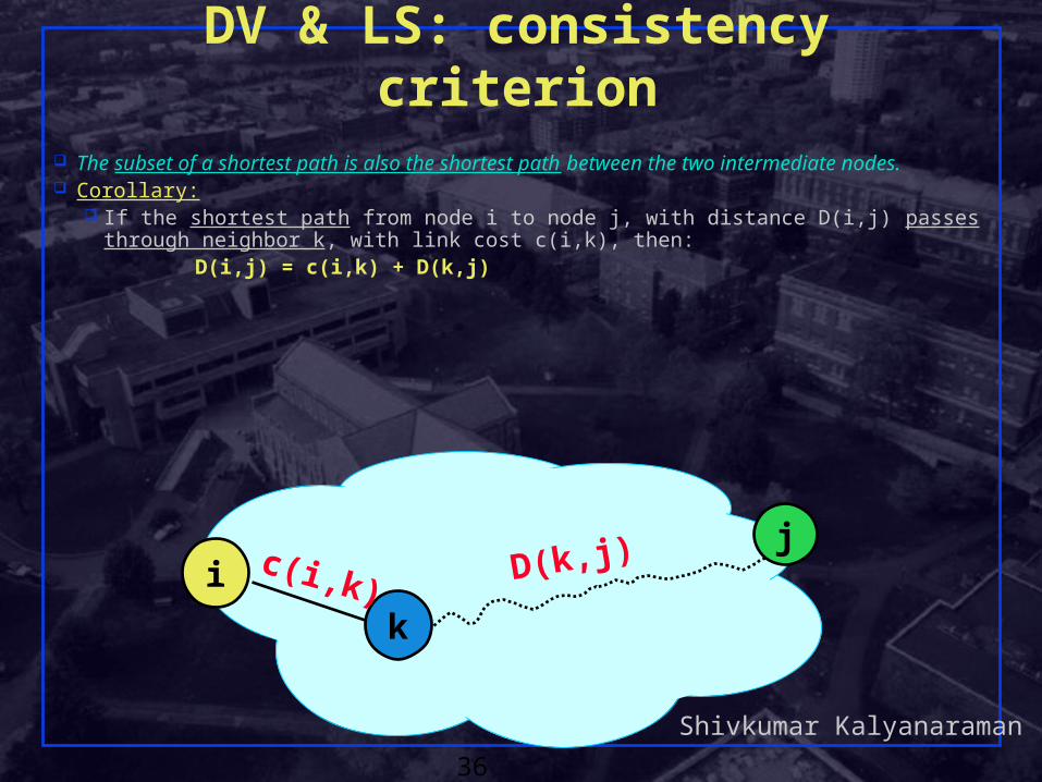
DV & LS: consistency criterion The subset of a shortest path is also the shortest path between the two intermediate nodes. Corollary:

If the shortest path from node i to node j, with distance D(i,j) passes through neighbor k, with link cost c(i,k), then:

D(i,j) = c(i,k) + D(k,j)

i

k

jc(i,k)

D(k,j)


37

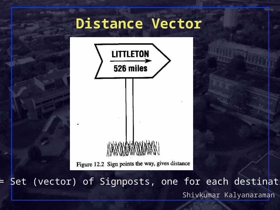
Distance Vector

DV = Set (vector) of Signposts, one for each destination


38

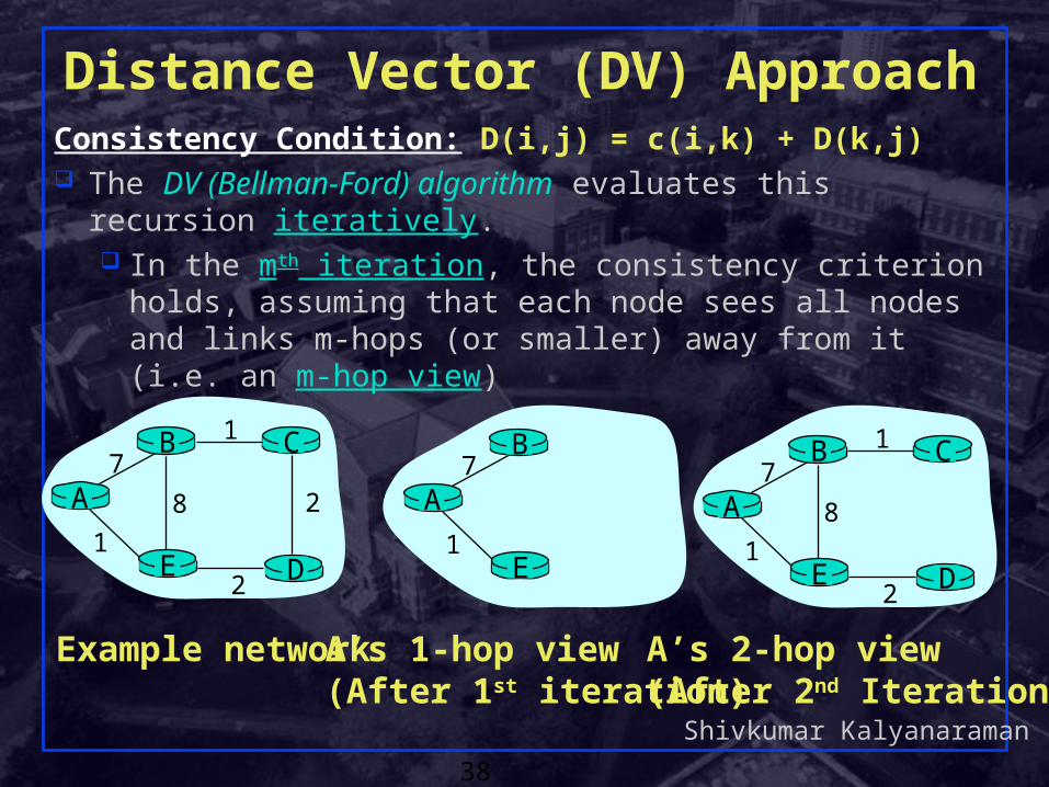
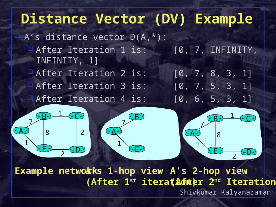
Distance Vector (DV) ApproachConsistency Condition: D(i,j) = c(i,k) + D(k,j) The DV (Bellman-Ford) algorithm evaluates this recursion

iteratively. In the mth iteration, the consistency criterion holds,

assuming that each node sees all nodes and links m-hops (or smaller) away from it (i.e. an m-hop view)

A

E D

CB7

8

1

2

1

2

Example network

A

E D

CB7

8

1

2

1

A’s 2-hop view(After 2nd Iteration)

A

E

B7

1

A’s 1-hop view(After 1st iteration)


39

Distance Vector (DV)… Initial distance values (iteration 1):

D(i,i) = 0 ; D(i,k) = c(i,k) if k is a neighbor (i.e. k is one-hop

away); and D(i,j) = INFINITY for all other non-neighbors j.

Note that the set of values D(i,*) is a distance vector at node i.

The algorithm also maintains a next-hop value (forwarding table) for every destination j, initialized as: next-hop(i) = i; next-hop(k) = k if k is a neighbor, and next-hop(j) = UNKNOWN if j is a non-neighbor.


40

Distance Vector (DV).. (Cont’d)

After every iteration each node i exchanges its distance vectors D(i,*) with its immediate neighbors.

For any neighbor k, if c(i,k) + D(k,j) < D(i,j), then: D(i,j) = c(i,k) + D(k,j) next-hop(j) = k

After each iteration, the consistency criterion is met After m iterations, each node knows the shortest path

possible to any other node which is m hops or less. I.e. each node has an m-hop view of the network. The algorithm converges (self-terminating) in O(d)

iterations: d is the maximum diameter of the network.


41

Distance Vector (DV) Example A’s distance vector D(A,*):

After Iteration 1 is: [0, 7, INFINITY, INFINITY, 1] After Iteration 2 is: [0, 7, 8, 3, 1] After Iteration 3 is: [0, 7, 5, 3, 1] After Iteration 4 is: [0, 6, 5, 3, 1]

A

E D

CB7

8

1

2

1

2

Example network

A

E D

CB7

8

1

2

1

A’s 2-hop view(After 2nd Iteration)

A

E

B7

1

A’s 1-hop view(After 1st iteration)


42

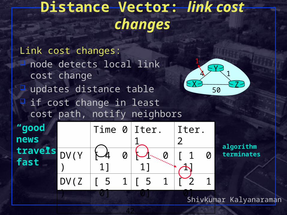
Distance Vector: link cost changes

Link cost changes: node detects local link cost change updates distance table if cost change in least cost path,

notify neighbors

X Z14

50

Y1

algorithmterminates

“goodnews travelsfast”

Time 0 Iter. 1 Iter. 2

DV(Y) [ 4 0 1] [ 1 0 1] [ 1 0 1]

DV(Z) [ 5 1 0] [ 5 1 0] [ 2 1 0]


43

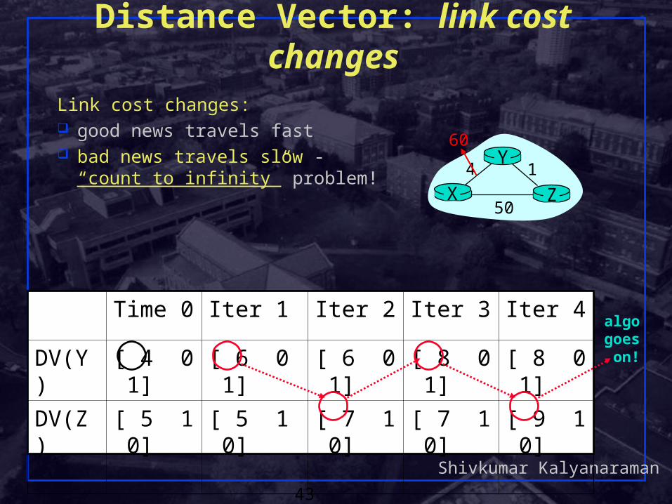
Distance Vector: link cost changesLink cost changes: good news travels fast bad news travels slow - “count to

infinity” problem! X Z14

50

Y60

algogoes

on!

Time 0 Iter 1 Iter 2 Iter 3 Iter 4

DV(Y) [ 4 0 1] [ 6 0 1] [ 6 0 1] [ 8 0 1] [ 8 0 1]

DV(Z) [ 5 1 0] [ 5 1 0] [ 7 1 0] [ 7 1 0] [ 9 1 0]


44

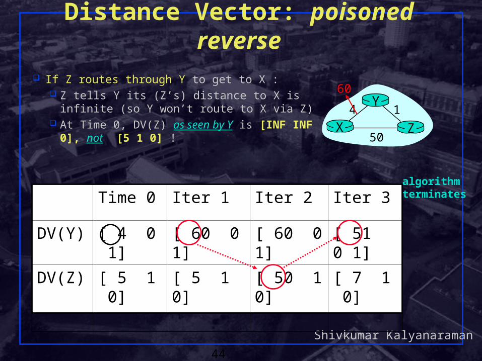
Distance Vector: poisoned reverse If Z routes through Y to get to X :

Z tells Y its (Z’s) distance to X is infinite (so Y won’t route to X via Z)

At Time 0, DV(Z) as seen by Y is [INF INF 0], not [5 1 0] !

X Z14

50

Y60

algorithmterminatesTime 0 Iter 1 Iter 2 Iter 3

DV(Y) [ 4 0 1] [ 60 0 1] [ 60 0 1] [ 51 0 1]

DV(Z) [ 5 1 0] [ 5 1 0] [ 50 1 0] [ 7 1 0]


45

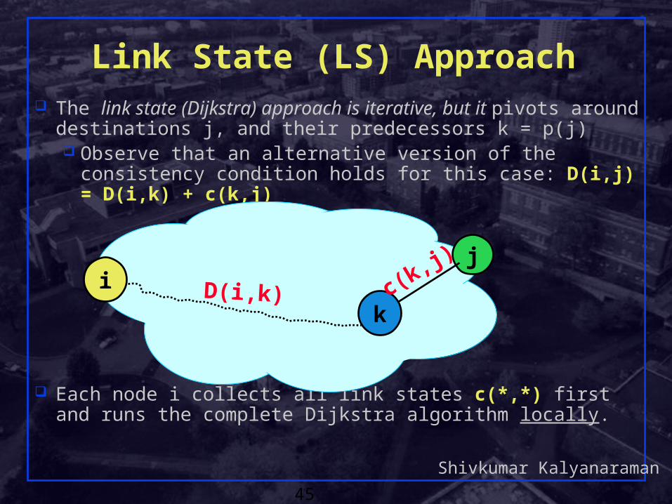
Link State (LS) Approach The link state (Dijkstra) approach is iterative, but it pivots

around destinations j, and their predecessors k = p(j) Observe that an alternative version of the consistency

condition holds for this case: D(i,j) = D(i,k) + c(k,j)

Each node i collects all link states c(*,*) first and runs the complete Dijkstra algorithm locally.

i

k

jc(k

,j)

D(i,k)


46

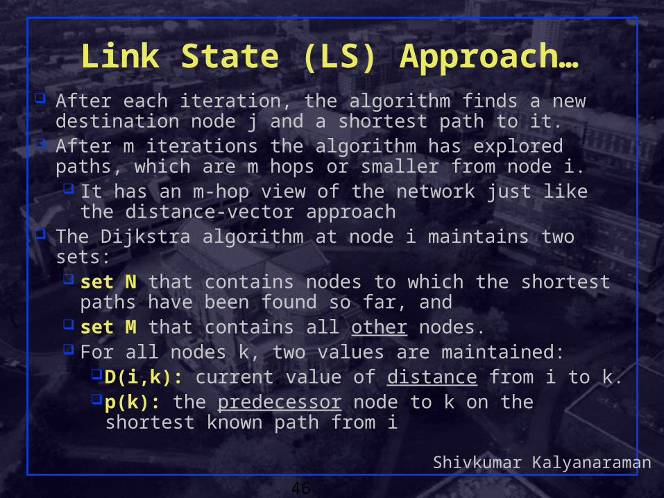
Link State (LS) Approach… After each iteration, the algorithm finds a new destination

node j and a shortest path to it. After m iterations the algorithm has explored paths, which are

m hops or smaller from node i. It has an m-hop view of the network just like the distance-

vector approach The Dijkstra algorithm at node i maintains two sets:

set N that contains nodes to which the shortest paths have been found so far, and

set M that contains all other nodes. For all nodes k, two values are maintained:

D(i,k): current value of distance from i to k. p(k): the predecessor node to k on the shortest known

path from i


47

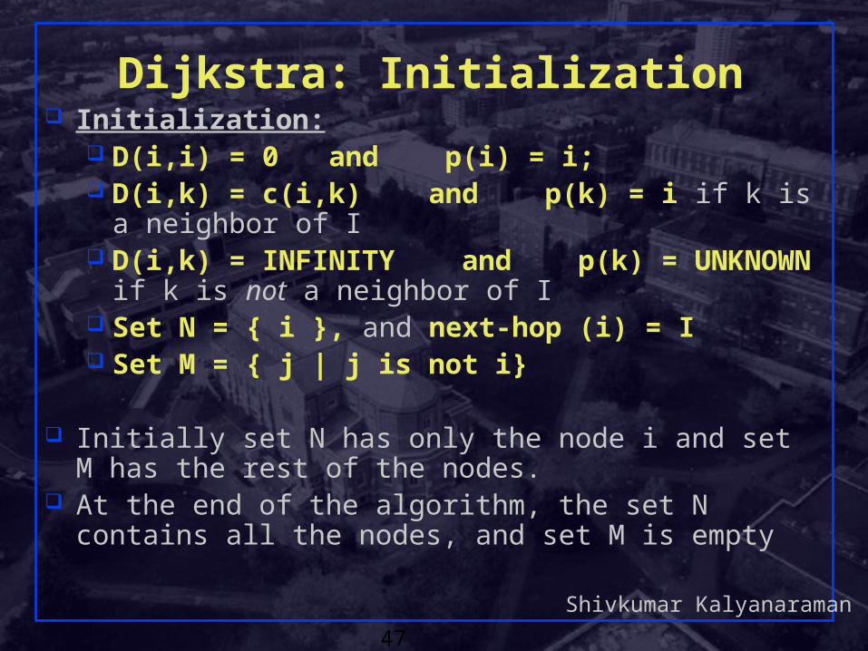
Dijkstra: Initialization Initialization:

D(i,i) = 0 and p(i) = i; D(i,k) = c(i,k) and p(k) = i if k is a neighbor of I D(i,k) = INFINITY and p(k) = UNKNOWN if k is

not a neighbor of I Set N = { i }, and next-hop (i) = I Set M = { j | j is not i}

Initially set N has only the node i and set M has the rest of the nodes.

At the end of the algorithm, the set N contains all the nodes, and set M is empty


48

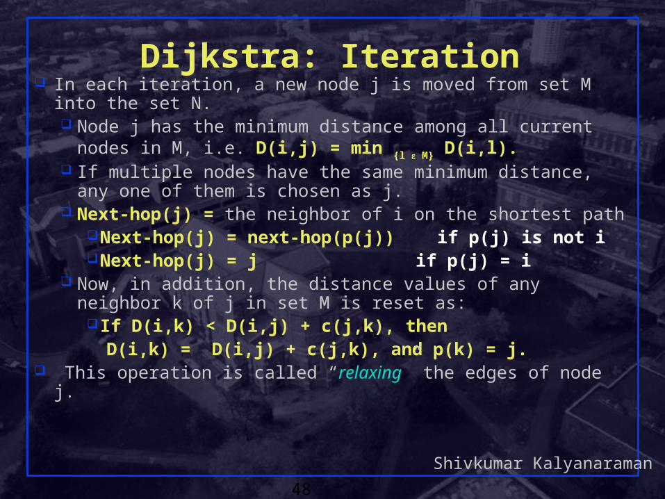
Dijkstra: Iteration In each iteration, a new node j is moved from set M into the set

N. Node j has the minimum distance among all current nodes

in M, i.e. D(i,j) = min {l M} D(i,l). If multiple nodes have the same minimum distance, any one

of them is chosen as j. Next-hop(j) = the neighbor of i on the shortest path

Next-hop(j) = next-hop(p(j)) if p(j) is not iNext-hop(j) = j if p(j) = i

Now, in addition, the distance values of any neighbor k of j in set M is reset as:

If D(i,k) < D(i,j) + c(j,k), then D(i,k) = D(i,j) + c(j,k), and p(k) = j. This operation is called “relaxing” the edges of node j.


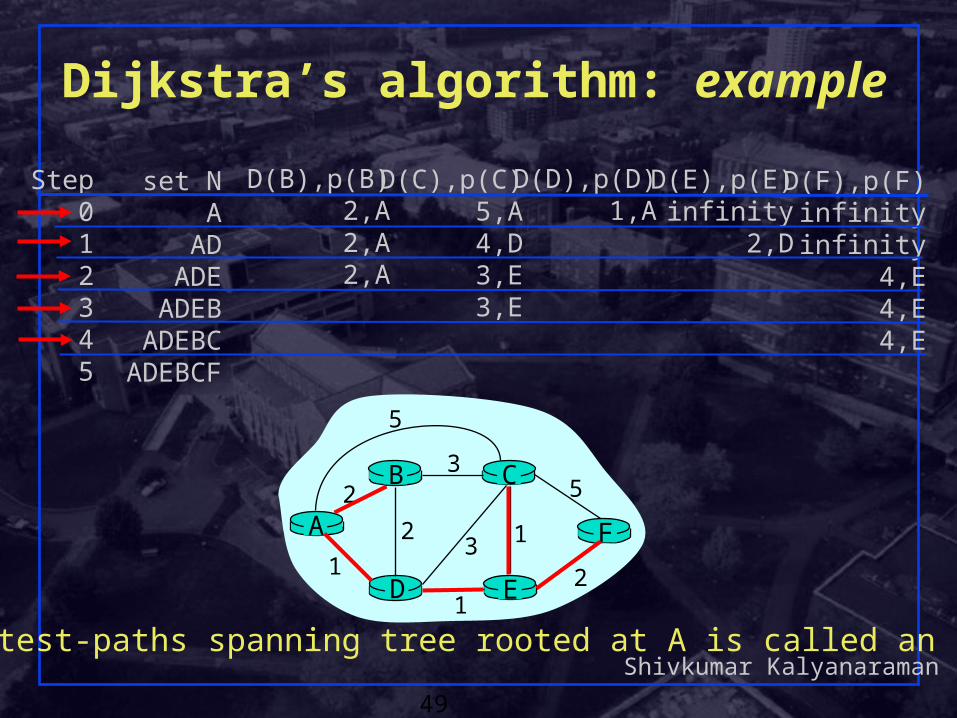
49

Dijkstra’s algorithm: example

Step012345

set NA

ADADE

ADEBADEBC

ADEBCF

D(B),p(B)2,A2,A2,A

D(C),p(C)5,A4,D3,E3,E

D(D),p(D)1,A

D(E),p(E)infinity

2,D

D(F),p(F)infinityinfinity

4,E4,E4,E

A

ED

CB

F

2

2

13

1

1

2

53

5

The shortest-paths spanning tree rooted at A is called an SPF-tree


50

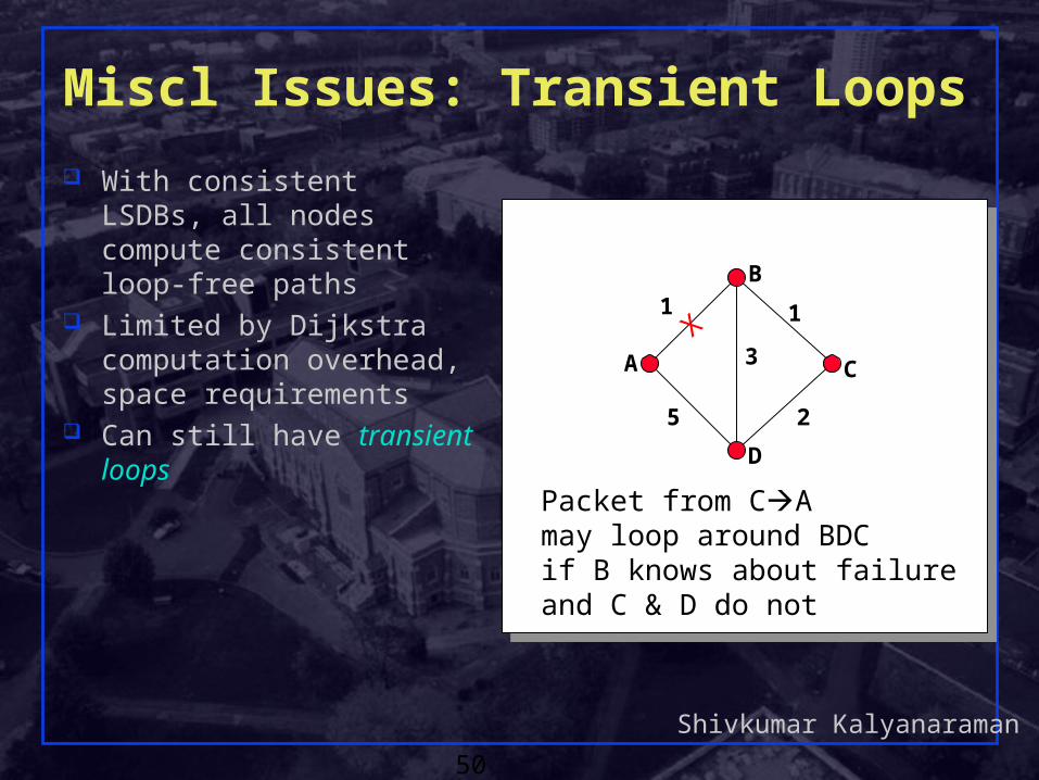
Miscl Issues: Transient Loops

With consistent LSDBs, all nodes compute consistent loop-free paths

Limited by Dijkstra computation overhead, space requirements

Can still have transient loops

A

B

C

D

1

3

5 2

1

Packet from CAmay loop around BDCif B knows about failureand C & D do not

X


51

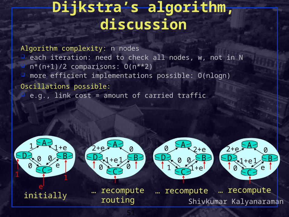
Dijkstra’s algorithm, discussion

Algorithm complexity: n nodes each iteration: need to check all nodes, w, not in N n*(n+1)/2 comparisons: O(n**2) more efficient implementations possible: O(nlogn)

Oscillations possible: e.g., link cost = amount of carried traffic

A

D

C

B1 1+e

e0

e

1 1

0 0

A

D

C

B2+e 0

001+e1

A

D

C

B0 2+e

1+e10 0

A

D

C

B2+e 0

e01+e1

initially… recompute

routing… recompute … recompute


52

Misc: How to assign the Cost Metric? Choice of link cost defines traffic load

Low cost = high probability link belongs to SPT and will attract traffic

Tradeoff: convergence vs load distribution Avoid oscillations Achieve good network utilization

Static metrics (weighted hop count) Does not take traffic load (demand) into account.

Dynamic metrics (cost based upon queue or delay etc) Highly oscillatory, very hard to dampen (DARPAnet

experience) Quasi-static metric:

Reassign static metrics based upon overall network load (demand matrix), assumed to be quasi-stationary


53

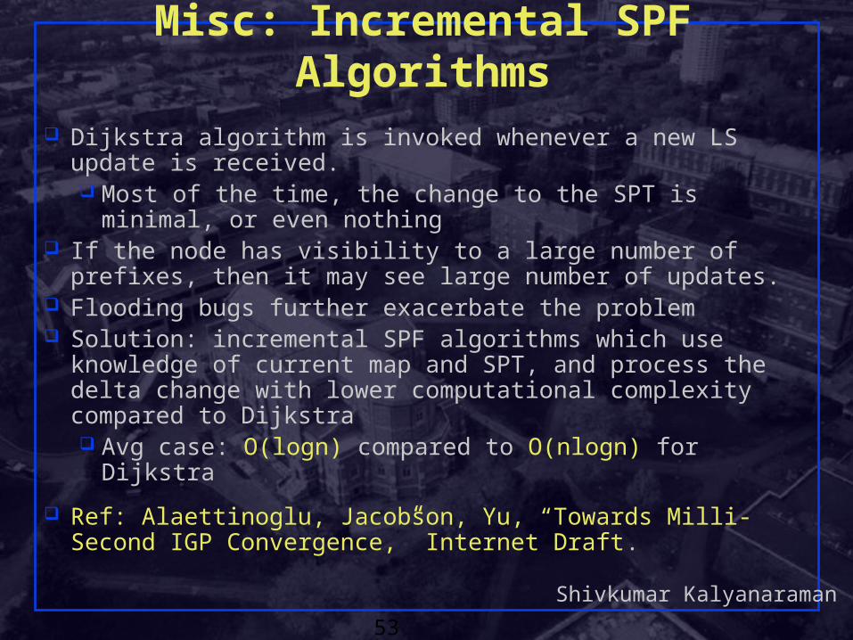
Misc: Incremental SPF Algorithms Dijkstra algorithm is invoked whenever a new LS update is

received. Most of the time, the change to the SPT is minimal, or

even nothing If the node has visibility to a large number of prefixes, then

it may see large number of updates. Flooding bugs further exacerbate the problem Solution: incremental SPF algorithms which use knowledge

of current map and SPT, and process the delta change with lower computational complexity compared to Dijkstra Avg case: O(logn) compared to O(nlogn) for Dijkstra

Ref: Alaettinoglu, Jacobson, Yu, “Towards Milli-Second IGP Convergence,” Internet Draft.


54

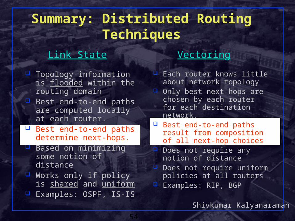
Topology information is flooded within the routing domain

Best end-to-end paths are computed locally at each router.

Best end-to-end paths determine next-hops.

Based on minimizing some notion of distance

Works only if policy is shared and uniform

Examples: OSPF, IS-IS

Each router knows little about network topology

Only best next-hops are chosen by each router for each destination network.

Best end-to-end paths result from composition of all next-hop choices

Does not require any notion of distance

Does not require uniform policies at all routers

Examples: RIP, BGP

Link State Vectoring

Summary: Distributed Routing Techniques


55

Routing vs Forwarding Forwarding table vs Forwarding in simple topologies Routers vs Bridges: review Routing Problem Telephony vs Internet Routing Source-based vs Fully distributed Routing Distance vector vs Link state routing

Bellman Ford and Dijkstra Algorithms

Addressing and Routing: Scalability

Where are we?


56

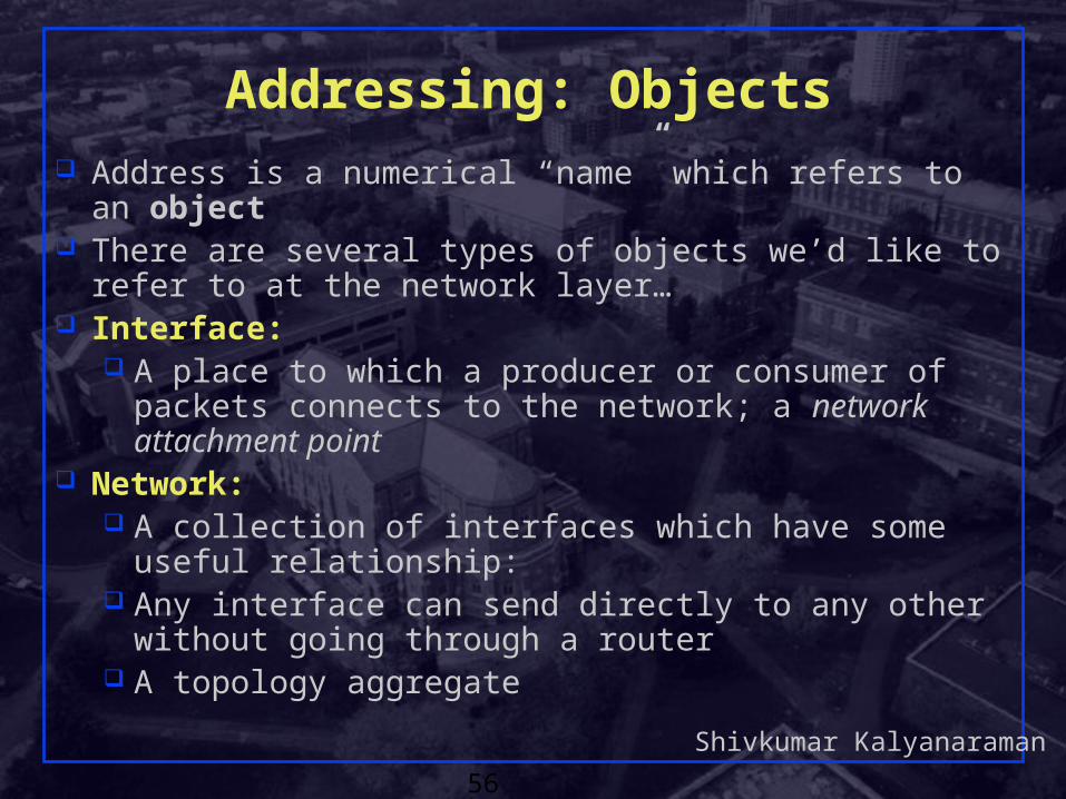
Addressing: Objects Address is a numerical “name” which refers to an object There are several types of objects we’d like to refer to at

the network layer… Interface:

A place to which a producer or consumer of packets connects to the network; a network attachment point

Network: A collection of interfaces which have some useful

relationship: Any interface can send directly to any other without

going through a router A topology aggregate


57

Addressing: Objects

Route or Path: A path from one place in the network to another

Host: An actual machine which is the source or destination

of traffic, through some interface Router:

A device which is interconnecting various elements of the network, and forwarding traffic

Node: A host or router


58

Address Concept Address: A structured name for a network interface or topology

aggregate: The structure is used by the routing to help it scale Topologically related items have to be given related addresses Topologically related addresses also:

Allow the number of destinations tracked by the routing to be minimized

Allow quick location of the named interface on a map Provide a representation for topology distribution Provide a framework for the abstraction process

DNS names: A structured human usable name for a host, etc The structure facilitates the distribution and lookup


59

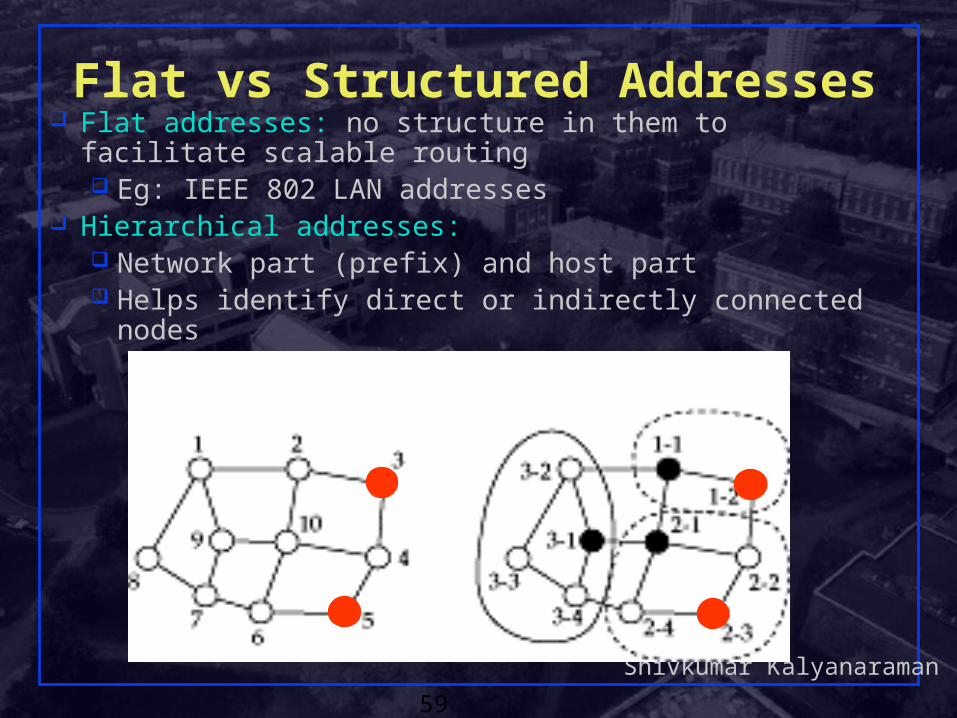
Flat vs Structured Addresses Flat addresses: no structure in them to facilitate scalable

routing Eg: IEEE 802 LAN addresses

Hierarchical addresses: Network part (prefix) and host part Helps identify direct or indirectly connected nodes


60

Tradeoffs in Large Scale Routing Tradeoff: discard detailed routing information vs incur the

overhead of large, potentially unneeded detail. This process is called abstraction.

There are two types of abstraction for routing: Compression, in which the same routing decision is

made in all cases after the abstraction as before Thinning, in which the routing is affected If the prior routing was optimal, discarding routing

information via thinning means non-optimal routes Large-scale routing incurs two kinds of overhead cost:

The cost of running the routing The cost of non-optimal routes Challenge of routing is managing this choice of costs.


61

Hierarchical Routing Example: PNNI


62

Summary

Routing Concepts DV and LS algorithms Addressing and Hierarchy

Documents

Shivkumar Kalyanaraman 1 Routing I: Basic Ideas Shivkumar Kalyanaraman Rensselaer Polytechnic Institute [email protected] Based in part upon slides