Embed Size (px)
Citation preview
Vol. 21 (2005) 598–642
www.elsevier.com/locate/ejpe
Shadow economies around the world:
what do we really know?
Friedrich Schneider*
Department of Economics, Johannes Kepler University of Linz, A-4040 Linz-Auhof, Austria
Received 16 February 2004; received in revised form 6 July 2004; accepted 11 October 2004
Available online 15 December 2004
Abstract
This paper presents estimates of the shadow economy for 110 countries, including developing,
transition and developed OECD economies. The average size of the shadow economy as a
proportion of official GDP in 1999–2000 in developing countries was 41%, in transition countries
38%, and in OECD countries 17%. An increasing burden of taxation and social security
contributions underlies the shadow economy. If the shadow economy increases by 1%, the growth
rate of the bofficialQ GDP of developing countries decreases by 0.6%, while in developed and
transition economies the shadow economy respectively increases by 0.8% and 1.0%.
D 2004 Elsevier B.V. All rights reserved.
JEL classification: O17; O5; D78; H2; H11; H26
Keywords: Shadow economy; Tax burden; Regulation; DYMIMIC method
1. Introduction
Shadow economic activities are a fact of life around the world. Most societies attempt
to control these activities through measures such as punishment and prosecution, or by
relying on economic growth or education. Gathering statistics about who is engaged in
shadow economy activities and the frequencies with which these activities occur and
magnitudes, is important. It is difficult to obtain accurate information because individuals
0176-2680/$ -
doi:10.1016/j.e
* Tel.: +43 7
E-mail add
European Journal of Political Economy
see front matter D 2004 Elsevier B.V. All rights reserved.
jpoleco.2004.10.002
32 2468 8210; fax: +43 732 2468 28210.
ress: [email protected].
F. Schneider / European Journal of Political Economy 21 (2005) 598–642 599
engaged in shadow economy activities do not wish to be identified. Hence, the estimation
of shadow-economy activities is a scientific passion for knowing the unknown. Although
there is quite a large literature on particular aspects of the hidden or shadow economy and
a comprehensive survey exists,1 the subject remains controversial.2 There are disagree-
ments about the definition of shadow-economy activities, the appropriate estimation
procedures, and the use of the estimates in economic analysis and policy.3 Around the
world, there are some indications of increases in shadow economies but little is precisely
known about the size of shadow economies in transition, low-income, and high-income
countries over the period 1990–2000. The goals of this paper are (1) to estimate the
shadow economy for 110 countries, (2) to provide insights about the main causes of the
shadow economy, and (3) to study the dynamic effects of the shadow economy on the
official economy. Section 2 defines the shadow economy and theoretical considerations
about why the shadow economy is increasing are proposed. Section 3 presents the
empirical results. Section 4 presents the dynamic effects of the shadow economy on the
official economy. Section 5 summarizes and suggests policy conclusions. The appendices
set out the various methods for estimating the shadow economy and describe the data.
Some further econometric results are also shown.
2. Theoretical considerations
2.1. Defining the shadow economy
Researchers attempting to measure the size of shadow economy face the question of the
definition. One commonly used working definition is all currently unregistered economic
activities that contribute to the officially calculated (or observed) Gross National Product.4
Smith (1994, p. 18) uses the definition bmarket-based production of goods and services,
whether legal or illegal, that escapes detection in the official estimates of GDP.Q One of thebroadest definitions includes bthose economic activities and the income derived from them
that circumvent or other wise government regulation, taxation or observationQ.5 As thesedefinitions still leave open a lot of questions, Table 2.1 is helpful for developing a feeling
for what could be a reasonable consensus definition of the underground (or shadow)
economy. From Table 2.1, it is clear that a broad definition of the shadow economy
includes unreported income from the production of legal goods and services, either from
1 See Frey and Pommerehne (1984), Thomas (1992), Loayza (1996), Pozo (1996), Lippert and Walker (1997),
Schneider (1994a,b, 1997, 1998a), Johnson et al. (1997, 1998a), Belev (2003), Gerxhani (2003), and Pedersen
(2003). For surveys of evidence, see Schneider and Enste (2000, 2002), Schneider (2003) and Alm et al. (2004).2 See the Economic Journal, vol. 109, June 1999.3 Compare the different opinions of Tanzi (1999), Thomas (1999), Giles (1999a,b) and Pedersen (2003).4 This definition is used, for example, by Feige (1989, 1994), Schneider (1994a, 2003), and Frey and
Pommerehne (1984). Do-it-yourself activities are not included. For estimates of the shadow economy and do-it-
yourself activities for Germany, see 5This definition is taken from Del’Anno (2003), Del’Anno and Schneider
(2004) and Feige (1989). See also Thomas (1999) and Fleming et al. (2000).Karmann (1990).5 This definition is taken from Del’Anno (2003), Del’Anno and Schneider (2004) and Feige (1989). See also
Thomas (1999) and Fleming et al. (2000).
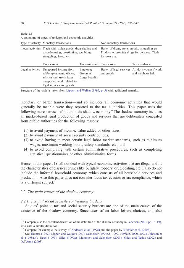
Table 2.1
A taxonomy of types of underground economic activities
Type of activity Monetary transactions Non-monetary transactions
Illegal activities Trade with stolen goods; drug dealing and
manufacturing; prostitution; gambling;
smuggling; fraud; etc.
Barter of drugs, stolen goods, smuggling etc.
Produce or growing drugs for own use. Theft
for own use.
Tax evasion Tax avoidance Tax evasion Tax avoidance
Legal activities Unreported income from
self-employment; Wages,
salaries and assets from
unreported work related to
legal services and goods
Employee
discounts,
fringe benefits
Barter of legal services
and goods
All do-it-yourself work
and neighbor help
Structure of the table is taken from Lippert and Walker (1997, p. 5) with additional remarks.
F. Schneider / European Journal of Political Economy 21 (2005) 598–642600
monetary or barter transactions—and so includes all economic activities that would
generally be taxable were they reported to the tax authorities. This paper uses the
following more narrow definition of the shadow economy.6 The shadow economy includes
all market-based legal production of goods and services that are deliberately concealed
from public authorities for the following reasons:
(1) to avoid payment of income, value added or other taxes,
(2) to avoid payment of social security contributions,
(3) to avoid having to meet certain legal labor market standards, such as minimum
wages, maximum working hours, safety standards, etc., and
(4) to avoid complying with certain administrative procedures, such as completing
statistical questionnaires or other administrative forms.
Hence, in this paper, I shall not deal with typical economic activities that are illegal and fit
the characteristics of classical crimes like burglary, robbery, drug dealing, etc. I also do not
include the informal household economy, which consists of all household services and
production. Also this paper does not consider focus tax evasion or tax compliance, which
is a different subject.7
2.2. The main causes of the shadow economy
2.2.1. Tax and social security contribution burdens
Studies8 point to tax and social security burdens are one of the main causes of the
existence of the shadow economy. Since taxes affect labor–leisure choices, and also
6 Compare also the excellent discussion of the definition of the shadow economy in Pedersen (2003, pp.13–19),
who uses a similar definition.7 Compare for example the survey of Andreoni et al. (1998) and the paper by Kirchler et al. (2002).8 See Thomas (1992); Lippert and Walker (1997); Schneider (1994a,b, 1997, 1998a,b, 2000, 2003); Johnson et
al. (1998a,b); Tanzi (1999); Giles (1999a); Mummert and Schneider (2001); Giles and Tedds (2002) and
Del’Anno (2003).
F. Schneider / European Journal of Political Economy 21 (2005) 598–642 601
increase labor supply in the shadow economy, the distortion of the overall tax
burden is a major concern. The greater the difference between the total cost of labor
in the official economy and after-tax earnings from work, the greater is the incentive
to work in the shadow economy. However, even major tax reforms with major tax
rate deductions may not lead to a substantial decrease of the shadow economy.9
Such reforms may stabilize the size of the shadow economy and avoid a further
increase. Social networks and personal relationships, high profits from irregular
activities, and associated investments in real and human capital prevent people from
transferring to the official economy. For Canada, Spiro (1993) found such reactions
of people facing an increase in indirect taxes (VAT, GST). This reduces incentives
for politicians to carry out major reforms because they may not gain a lot from
them.
Empirical studies of the influence of the tax burden on the shadow economy by
Schneider (1994b, 2000) and Johnson et al. (1998a,b) show statistically significant
evidence for the influence of taxation on the shadow economy. A strong influence of
indirect and direct taxation on the shadow economy is further demonstrated by empirical
results for Austria and the Scandinavian countries. For Austria the driving force for the
shadow economy is the direct tax burden (including social security payments), which
has the greatest influence, followed by the intensity of regulation and complexity of the
tax system. A similar conclusion was reached (Schneider, 1986) for the Scandinavian
countries where tax variables (average direct tax rate, average total tax rate (indirect and
direct tax rate)) and marginal tax rates had the expected positive sign on currency
demand and were highly statistically significant. These findings are supported by studies
by Kirchgassner (1983, 1984) for Germany and Klovland (1984) for Norway and
Sweden.
Here I investigate the influence of the direct and indirect tax burden as well as social
security payments on the shadow economy for developing, transition and rich countries.
For the first time this influence is investigated for the same time period and using the same
estimation technique.
2.2.2. Intensity of regulation
The increase in the intensity of regulation, often measured in the numbers of laws and
regulations, is another important factor that reduces the freedom of choice for individuals
engaged in the official economy.10 One can think of labor market regulations, trade
barriers, and labor restrictions for foreigners. Johnson et al. (1998b) find overall significant
empirical evidence of the influence of labor regulations on the shadow economy (the
impact is clearly described and theoretically derived in other studies, e.g. for Germany,
Deregulation Commission 1990/1991). Regulation substantially increases labor costs in
9 See Schneider (1994b, 1998b) for a similar result of the effects of a major tax reform in Austria on the shadow
economy. I show that a major reduction in the direct tax burden did not lead to a major reduction in the size of the
shadow economy. Legal tax avoidance was abolished and other aspects of regulations were not changed; hence
for a considerable part of taxpayers, the actual tax and regulation burden remained unchanged.10 See for a (social) psychological theoretical foundation of this feature, Brehm (1966, 1972), and for a (first)
application to the shadow economy, Pelzmann (1988).
F. Schneider / European Journal of Political Economy 21 (2005) 598–642602
the official economy but, since most of these costs can be shifted onto employees, these
costs provide another incentive to work in the shadow economy where they can be
avoided. Johnson et al. (1997) confirm the prediction that countries with greater
regulation of their economies tend to have a higher share of the unofficial
economy relative to GDP. A 1-point increase of the regulation index (ranging from
1 to 5, with 5 the most regulation) is ceteris paribus associated with an 8.1
percentage point increase in the share of the shadow economy, when controlled for
GDP per capita (Johnson et. al., 1998b, p. 18). They conclude that it is the
enforcement of regulation that is the key factor for the burden on firms and
individuals, and not the overall extent of regulation—mostly not enforced—that
drives firms into the shadow economy. Friedman et al. (2000) reach a similar
result. In their study every available measure of regulation is significantly correlated
with the share of the unofficial economy and the sign of the relationship is
unambiguous: more regulation is correlated with a larger shadow economy. A one
point increase in an index of regulation (ranging from 1 to 5) is associated with a
10% increase in the shadow economy for 76 developing, transition and developed
countries.
These findings demonstrate that governments should place more emphasis on
improving enforcement of laws and regulations rather than increasing their number.
Some governments, however, prefer a policy of more regulations and laws when trying to
reduce the shadow economy, mostly because it leads to an increase in power of the
bureaucrats and to higher employment in the public sector.
2.2.3. Public sector services
An increase in the size of the shadow economy can lead to reduced state revenues,
which in turn reduces the quality and quantity of publicly provided goods and services.
Ultimately, this can lead to an increase in tax rates for firms and individuals in the
official sector, quite often combined with a deterioration in the quality of public goods
(such as infrastructure) and of administration, with the consequence of even stronger
incentives to participate in the shadow economy. Johnson et al. (1998a,b) present a
simple model of this relationship. Their findings show that smaller shadow economies
appear in countries with higher tax revenues, if achieved by lower tax rates, fewer laws
and regulations and less bribery facing enterprises. Countries with better rule of the
law, which is financed by tax revenues, also have smaller shadow economies.
Transition countries have higher levels of regulation, leading to a significantly higher
incidence of bribery, higher effective taxes on official activities, and a large
discretionary framework of regulations, and consequently to a higher shadow economy.
Their overall conclusion is that bwealthier countries of the OECD, as well as some in
Eastern Europe find themselves in the dgood equilibriumT of relatively low tax and
regulatory burden, sizeable revenue mobilization, good rule of law and corruption
control, and [relatively] small unofficial economy. By contrast, a number of countries
in Latin American and the former Soviet Union exhibit characteristics consistent with a
dbad equilibriumT: tax and regulatory discretion and burden on the firm are high, the
rule of law is weak, and there is a high incidence of bribery and a relatively high share
of activities in the unofficial economyQ (Johnson et al., 1998a). Unfortunately, due to
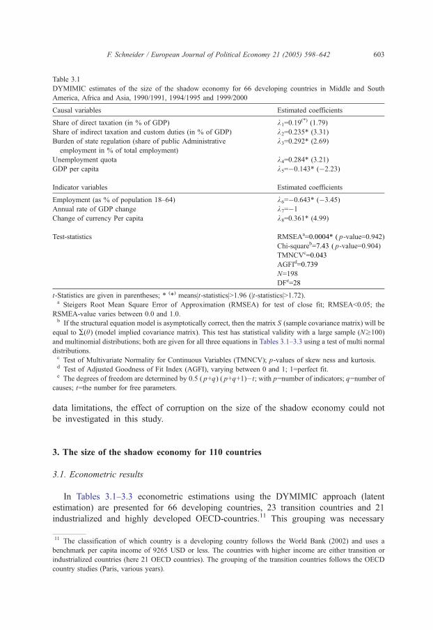
Table 3.1
DYMIMIC estimates of the size of the shadow economy for 66 developing countries in Middle and South
America, Africa and Asia, 1990/1991, 1994/1995 and 1999/2000
Causal variables Estimated coefficients
Share of direct taxation (in % of GDP) k1=0.19(*) (1.79)
Share of indirect taxation and custom duties (in % of GDP) k2=0.235* (3.31)
Burden of state regulation (share of public Administrative
employment in % of total employment)
k3=0.292* (2.69)
Unemployment quota k4=0.284* (3.21)
GDP per capita k5=�0.143* (�2.23)
Indicator variables Estimated coefficients
Employment (as % of population 18–64) k6=�0.643* (�3.45)
Annual rate of GDP change k7=�1
Change of currency Per capita k8=0.361* (4.99)
Test-statistics RMSEAa=0.0004* ( p-value=0.942)
Chi-squareb=7.43 ( p-value=0.904)
TMNCVc=0.043
AGFId=0.739
N=198
DFe=28
t-Statistics are given in parentheses; * (*) means|t-statistics|N1.96 (|t-statistics|N1.72).a Steigers Root Mean Square Error of Approximation (RMSEA) for test of close fit; RMSEAb0.05; the
RSMEA-value varies between 0.0 and 1.0.b If the structural equation model is asymptotically correct, then the matrix S (sample covariance matrix) will be
equal to A(h) (model implied covariance matrix). This test has statistical validity with a large sample (Nz100)
and multinomial distributions; both are given for all three equations in Tables 3.1–3.3 using a test of multi normal
distributions.c Test of Multivariate Normality for Continuous Variables (TMNCV); p-values of skew ness and kurtosis.d Test of Adjusted Goodness of Fit Index (AGFI), varying between 0 and 1; 1=perfect fit.e The degrees of freedom are determined by 0.5 ( p+q) ( p+q+1)�t; with p=number of indicators; q=number of
causes; t=the number for free parameters.
F. Schneider / European Journal of Political Economy 21 (2005) 598–642 603
data limitations, the effect of corruption on the size of the shadow economy could not
be investigated in this study.
3. The size of the shadow economy for 110 countries
3.1. Econometric results
In Tables 3.1–3.3 econometric estimations using the DYMIMIC approach (latent
estimation) are presented for 66 developing countries, 23 transition countries and 21
industrialized and highly developed OECD-countries.11 This grouping was necessary
11 The classification of which country is a developing country follows the World Bank (2002) and uses a
benchmark per capita income of 9265 USD or less. The countries with higher income are either transition or
industrialized countries (here 21 OECD countries). The grouping of the transition countries follows the OECD
country studies (Paris, various years).
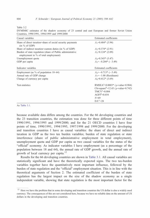
Table 3.2
DYMIMIC estimates of the shadow economy of 23 central and east European and former Soviet Union
Countries, 1990/1991, 1994/1995 and 1999/2000
Causal variables Estimated coefficients
Share of direct taxation+share of social security payments
(in % of GDP)
K1=0.484* (3.94)
Share of indirect taxation+custom duties (in % of GDP) K2=0.374* (2.91)
Burden of state regulation (share of Public administrative
employment in % of total employment)
K3=0.124* (2.09)
Unemployment quota K4=0.343* (3.47)
GDP per capita K5=�0.204* (�3.49)
Indicator variables Estimated coefficients
Employment (as % of population 18–64) K6=�0.713* (�5.49)
Annual rate of GDP change K7=�1.00 (Residuum)
Change of currency per capita K8=0.412* (3.69)
Test-statistics RMSEAa=0.0003* ( p-value=0.904)
Chi-squareb=12.43 ( p-value=0.742)
TMCVc=0.084
AGFId=0.654
N=69
D.F.c=28
As Table 3.1.
F. Schneider / European Journal of Political Economy 21 (2005) 598–642604
because available data differs among the countries. For the 66 developing countries and
the 23 transition countries, the estimation was done for three different points of time
1990/1991, 1994/1995 and 1999/2000; and for the 21 OECD countries I have four
points of time, 1990/1991, 1994/1995, 1997/1998 and 1999/2000. For the developing
and transition countries I have as causal variables: the share of direct and indirect
taxation in GDP as the two tax burden variables; burden of state regulation or state
interference (share of public administrative employment in total employment),
unemployment quota and GDP per capita as two causal variables for the status of the
bofficialQ economy. As indicator variables I have employment (as a percentage of the
population between 18 and 64), the annual rate of GDP growth, and the annual rate of
growth of local currency per capita.12
Results for the 66 developing countries are shown in Table 3.1. All causal variables are
statistically significant and have the theoretically expected signs. The two tax-burden
variables together have the quantitatively most important influence, followed by the
burden of state regulation and the bofficialQ employment situation. This is in line with the
theoretical arguments of Section 2. The estimated coefficient of the burden of state
regulation has the largest impact on the size of the shadow economy as a single
independent variable, showing that state regulation is the most important factor for the
12 Here we have the problem that in some developing and transition countries the US dollar is also a widely used
currency. The consequences of this are not considered here, because we have no reliable data on the amount of US
dollars in the developing and transition countries.
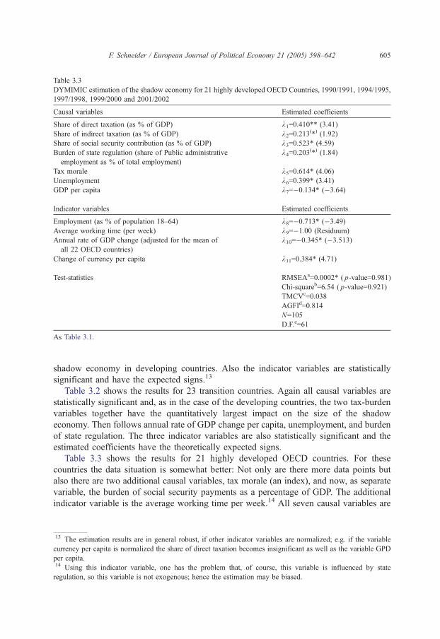
Table 3.3
DYMIMIC estimation of the shadow economy for 21 highly developed OECD Countries, 1990/1991, 1994/1995,
1997/1998, 1999/2000 and 2001/2002
Causal variables Estimated coefficients
Share of direct taxation (as % of GDP) k1=0.410** (3.41)
Share of indirect taxation (as % of GDP) k2=0.213(*) (1.92)
Share of social security contribution (as % of GDP) k3=0.523* (4.59)
Burden of state regulation (share of Public administrative
employment as % of total employment)
k4=0.203(*) (1.84)
Tax morale k5=0.614* (4.06)
Unemployment k6=0.399* (3.41)
GDP per capita k7=�0.134* (�3.64)
Indicator variables Estimated coefficients
Employment (as % of population 18–64) k8=�0.713* (�3.49)
Average working time (per week) k9=�1.00 (Residuum)
Annual rate of GDP change (adjusted for the mean of
all 22 OECD countries)
k10=�0.345* (�3.513)
Change of currency per capita k11=0.384* (4.71)
Test-statistics RMSEAa=0.0002* ( p-value=0.981)
Chi-squareb=6.54 ( p-value=0.921)
TMCVc=0.038
AGFId=0.814
N=105
D.F.e=61
As Table 3.1.
F. Schneider / European Journal of Political Economy 21 (2005) 598–642 605
shadow economy in developing countries. Also the indicator variables are statistically
significant and have the expected signs.13
Table 3.2 shows the results for 23 transition countries. Again all causal variables are
statistically significant and, as in the case of the developing countries, the two tax-burden
variables together have the quantitatively largest impact on the size of the shadow
economy. Then follows annual rate of GDP change per capita, unemployment, and burden
of state regulation. The three indicator variables are also statistically significant and the
estimated coefficients have the theoretically expected signs.
Table 3.3 shows the results for 21 highly developed OECD countries. For these
countries the data situation is somewhat better: Not only are there more data points but
also there are two additional causal variables, tax morale (an index), and now, as separate
variable, the burden of social security payments as a percentage of GDP. The additional
indicator variable is the average working time per week.14 All seven causal variables are
13 The estimation results are in general robust, if other indicator variables are normalized; e.g. if the variable
currency per capita is normalized the share of direct taxation becomes insignificant as well as the variable GPD
per capita.14 Using this indicator variable, one has the problem that, of course, this variable is influenced by state
regulation, so this variable is not exogenous; hence the estimation may be biased.
F. Schneider / European Journal of Political Economy 21 (2005) 598–642606
statistically significant and have the theoretically expected signs. The tax and social
security burden variables are quantitatively the most important, followed by the tax moral
variable, which has the single largest influence; hence taxpayers’ attitudes toward state
institutions/government are quite important in explaining whether people are engaged in
shadow economy activities. Also the official economy measured by unemployment and
GDP per capita has a quantitatively important influence on the shadow economy.
Turning to the four indicator variables, all have a statistically significant influence and
the estimated coefficients have the theoretically expected signs. The quantitatively most
important are employment and the change of currency per capita.15
Summarizing, the econometric results demonstrate that for all three groups of countries
the theoretical predictions of Section 2 are confirmed: The tax and social security payment
burden are the driving forces of the shadow economy, closely followed by the status of the
official economy for the developed and transition countries, and by the tax moral variable
for the highly developed OECD countries. For the developing countries the burden of state
regulation is the single most important factor.16
In order to calculate absolute values of the size of the shadow economies from these
DYMIMIC estimation results, I used the available estimates from the currency demand
approach in combination with the DYMIMIC approach for Australia, Austria, Germany,
Hungary, Italy, India, Peru, Russia and the United States (from studies of Chatterjee et
al., 2003; Del’Anno and Schneider, 2004; Bajada and Schneider, in press; Alexeev and
Pyle, 2003; Schneider and Enste, 2002; Lacko, 2000). Using values for the shadow
economy (as % of GDP) for these countries, the absolute values of the shadow
economy for all other countries could be calculated. The results are shown in the next
section.
3.2. The size of the shadow economies for 110 countries for 1990/1991, 1994/1995 and
1999/2000
When showing the size of the shadow economies over three periods of time in the
1990s for 110 countries that are quite different in location and stage of development, one
should be aware that such country comparisons provide only a very rough picture of the
ranking of the size of the shadow economy over the countries and over time. This is
because the DYMIMIC and the currency-demand methods have shortcomings, as
discussed in Appendix 1 (part 6.2); see also Thomas (1992, 1999), Tanzi (1999),
Pedersen (2003) and Ahumada et al. (2004). Due to these shortcomings and space reasons,
a detailed discussion of the (relative) ranking of the size of the shadow economy has not
been provided.
15 The variable currency per capita or annual change of currency per capita is heavily influenced by banking
innovations; hence this variable is quite unstable in the estimations with respect to the length of the estimation
period. Similar problems are mentioned by Giles (1999a) and Giles and Tedds (2002).16 In a sub-sample of 52 developing countries, corruption has the expected statistically significant positive
influence on the size of the shadow economy; however the quantitative importance is far below all other
independent variables (tax burden, state regulation, and statues of the official economy).
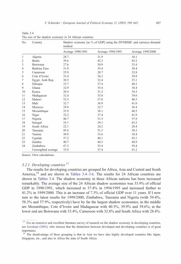
Table 3.4
The size of the shadow economy in 24 African countries
No. Shadow economy [as % of GDP] using the DYMIMIC and currency-demand
method
Country
Average 1990/1991 Average 1994/1995 Average 1999/2000
1 Algeria 28.7 31.9 34.1
2 Benin 39.6 42.3 45.2
3 Botswana 27.6 30.9 33.4
4 Burkina Faso 31.9 35.4 38.4
5 Cameroon 25.9 28.7 32.8
6 Cote d’Ivoire 33.4 36.2 39.9
7 Egypt, Arab Rep. 30.5 32.4 35.1
8 Ethiopia 33.7 37.4 40.3
9 Ghana 32.9 35.4 38.4
10 Kenya 28.4 31.2 34.3
11 Madagascar 32.4 35.8 39.6
12 Malawi 33.5 37.0 40.3
13 Mali 32.7 36.9 41.0
14 Morocco 29.8 32.7 36.4
15 Mozambique 35.9 38.1 40.3
16 Niger 32.2 37.4 41.9
17 Nigeria 46.7 51.5 57.9
18 Senegal 35.1 39.1 43.2
19 South Africa 22.1 24.2 28.4
20 Tanzania 45.6 51.3 58.3
21 Tunisia 30.9 33.6 38.4
22 Uganda 37.2 40.1 43.1
23 Zambia 40.7 44.3 48.9
24 Zimbabwe 47.3 53.4 59.4
Unweighted average 33.9 37.4 41.2
Source: Own calculations.
F. Schneider / European Journal of Political Economy 21 (2005) 598–642 607
3.2.1. Developing countries 17
The results for developing countries are grouped for Africa, Asia and Central and South
America,18 and are shown in Tables 3.4–3.6. The results for 24 African countries are
shown in Tables 3.4. The shadow economy in these African nations has been increased
remarkably. The average size of the 24 African shadow economies was 33.9% of official
GDP in 1990/1991, which increased to 37.4% in 1994/1995 and increased further to
41.2% in 1999/2000. This is an increase of 7.3% of official GDP over 11 years. If I now
turn to the latest results for 1999/2000, Zimbabwe, Tanzania and Nigeria (with 59.4%,
58.3% and 57.9%, respectively) have by far the largest shadow economies; in the middle
are Mozambique, Cote d’Ivoire and Madagascar with 40.3%, 39.9% and 39.6%; at the
lower end are Botswana with 33.4%, Cameroon with 32.8% and South Africa with 28.4%.
17 For an extensive and excellent literature survey of research on the shadow economy in developing countries,
see Gerxhani (2003), who stresses that the distinction between developed and developing countries is of great
importance.18 The disadvantage of these grouping is that in Asia we have also highly developed countries like Japan,
Singapore, etc., and also in Africa the state of South Africa.
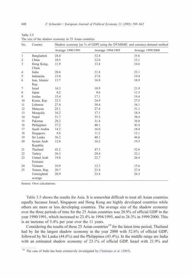
Table 3.5
The size of the shadow economy in 25 Asian countries
No. Country Shadow economy [as % of GDP] using the DYMIMIC and currency-demand method
Average 1990/1991 Average 1994/1995 Average 1999/2000
1 Bangladesh 28.4 32.4 35.6
2 China 10.5 12.0 13.1
3 Hong Kong,
China
11.9 13.4 16.6
4 India 20.6 21.8 23.1
5 Indonesia 15.4 17.6 19.4
6 Iran, Islamic
Rep.
13.7 16.8 18.9
7 Israel 16.3 18.9 21.9
8 Japan 8.2 9.6 11.3
9 Jordan 15.4 17.1 19.4
10 Korea, Rep. 22.3 24.9 27.5
11 Lebanon 27.4 30.4 34.1
12 Malaysia 25.1 27.4 31.1
13 Mongolia 16.2 17.1 18.4
14 Nepal 31.7 35.2 38.4
15 Pakistan 28.2 31.4 36.8
16 Philippines 37.2 40.1 43.4
17 Saudi Arabia 14.2 16.0 18.4
18 Singapore 9.8 11.2 13.1
19 Sri Lanka 36.2 40.1 44.6
20 Syrian Arab
Republic
12.8 16.2 19.3
21 Thailand 43.2 47.3 52.6
22 Turkey 26.3 29.4 32.1
23 United Arab
Emirates
19.8 22.7 26.4
24 Vietnam 10.9 12.3 15.6
25 Yemen, Rep. 20.7 23.4 27.4
Unweighted
average
20.9 23.4 26.3
Source: Own calculations.
F. Schneider / European Journal of Political Economy 21 (2005) 598–642608
Table 3.5 shows the results for Asia. It is somewhat difficult to treat all Asian countries
equally because Israel, Singapore and Hong Kong are highly developed countries while
others are more or less developing countries. The average size of the shadow economy
over the three periods of time for the 25 Asian countries was 20.9% of official GDP in the
year 1990/1991, which increased to 23.4% in 1994/1995, and to 26.3% in 1999/2000. This
is an increase of 5.4% per year over the 11 years.
Considering the results of these 25 Asian countries19 for the latest time period, Thailand
had by far the largest shadow economy in the year 2000 with 52.6% of official GDP;
followed by Sri Lanka (44.6%) and the Philippines (43.4%). In the middle range are India
with an estimated shadow economy of 23.1% of official GDP, Israel with 21.9% and
19 The case of India has been extensively investigated by Chatterjee et al. (2003).
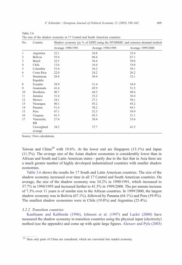
Table 3.6
The size of the shadow economy in 17 Central and South American countries
No. Country Shadow economy [as % of GDP] using the DYMIMIC and currency-demand method
Average 1990/1991 Average 1994/1995 Average 1999/2000
1 Argentina 22.1 24.8 25.4
2 Bolivia 55.4 60.4 67.1
3 Brazil 32.5 36.4 39.8
4 Chile 13.6 16.4 19.8
5 Colombia 33.4 36.2 39.1
6 Costa Rica 22.0 24.2 26.2
7 Dominican
Republic
28.4 30.4 32.1
8 Ecuador 28.9 31.4 34.4
9 Guatemala 41.4 45.9 51.5
10 Honduras 40.7 44.3 49.6
11 Jamaica 31.4 33.2 36.4
12 Mexico 24.1 27.1 30.1
13 Nicaragua 40.1 43.2 45.2
14 Panama 51.4 58.2 64.1
15 Peru 47.1 52.3 59.9
16 Uruguay 41.3 45.3 51.1
17 Venezuela,
RB
27.4 30.4 33.6
Unweighted
average
34.2 37.7 41.5
Source: Own calculations.
F. Schneider / European Journal of Political Economy 21 (2005) 598–642 609
Taiwan and China20 with 19.6%. At the lower end are Singapore (13.1%) and Japan
(11.3%). The average size of the Asian shadow economies is considerably lower than in
African and South and Latin American states—partly due to the fact that in Asia there are
a much greater number of highly developed industrialized countries with smaller shadow
economies.
Table 3.6 shows the results for 17 South and Latin American countries. The size of the
shadow economy increased over time in all 17 Central and South American countries. On
average, the size of the shadow economy was 34.2% in 1990/1991, which increased to
37.7% in 1994/1995 and increased further to 41.5% in 1999/2000. The per annum increase
of 7.3% over 11 years is of similar size to the African countries. In 1999/2000, the largest
shadow economy was in Bolivia (67.1%), followed by Panama (64.1%) and Peru (59.9%).
The smallest shadow economies were in Chile (19.8%) and Argentina (25.4%).
3.2.2. Transition countries
Kaufmann and Kaliberda (1996), Johnson et al. (1997) and Lacko (2000) have
measured the shadow economy in transition countries using the physical input (electricity)
method (see the appendix) and come up with quite large figures. Alexeev and Pyle (2003)
20 Here only parts of China are considered, which are converted into market economy.
F. Schneider / European Journal of Political Economy 21 (2005) 598–642610
and Belev (2003) critically evaluate the results and propose that the unofficial economies
are to a large content a historical phenomenon and partly determined by institutional
factors.
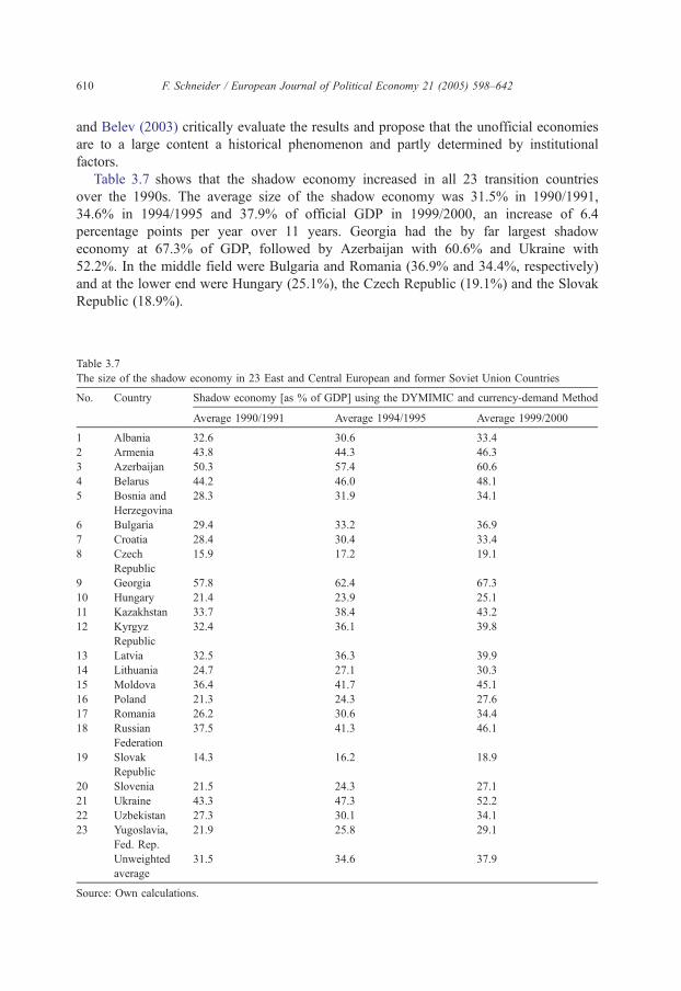
Table 3.7 shows that the shadow economy increased in all 23 transition countries
over the 1990s. The average size of the shadow economy was 31.5% in 1990/1991,
34.6% in 1994/1995 and 37.9% of official GDP in 1999/2000, an increase of 6.4
percentage points per year over 11 years. Georgia had the by far largest shadow
economy at 67.3% of GDP, followed by Azerbaijan with 60.6% and Ukraine with
52.2%. In the middle field were Bulgaria and Romania (36.9% and 34.4%, respectively)
and at the lower end were Hungary (25.1%), the Czech Republic (19.1%) and the Slovak
Republic (18.9%).
Table 3.7
The size of the shadow economy in 23 East and Central European and former Soviet Union Countries
No. Country Shadow economy [as % of GDP] using the DYMIMIC and currency-demand Method
Average 1990/1991 Average 1994/1995 Average 1999/2000
1 Albania 32.6 30.6 33.4
2 Armenia 43.8 44.3 46.3
3 Azerbaijan 50.3 57.4 60.6
4 Belarus 44.2 46.0 48.1
5 Bosnia and
Herzegovina
28.3 31.9 34.1
6 Bulgaria 29.4 33.2 36.9
7 Croatia 28.4 30.4 33.4
8 Czech
Republic
15.9 17.2 19.1
9 Georgia 57.8 62.4 67.3
10 Hungary 21.4 23.9 25.1
11 Kazakhstan 33.7 38.4 43.2
12 Kyrgyz
Republic
32.4 36.1 39.8
13 Latvia 32.5 36.3 39.9
14 Lithuania 24.7 27.1 30.3
15 Moldova 36.4 41.7 45.1
16 Poland 21.3 24.3 27.6
17 Romania 26.2 30.6 34.4
18 Russian
Federation
37.5 41.3 46.1
19 Slovak
Republic
14.3 16.2 18.9
20 Slovenia 21.5 24.3 27.1
21 Ukraine 43.3 47.3 52.2
22 Uzbekistan 27.3 30.1 34.1
23 Yugoslavia,
Fed. Rep.
21.9 25.8 29.1
Unweighted
average
31.5 34.6 37.9
Source: Own calculations.
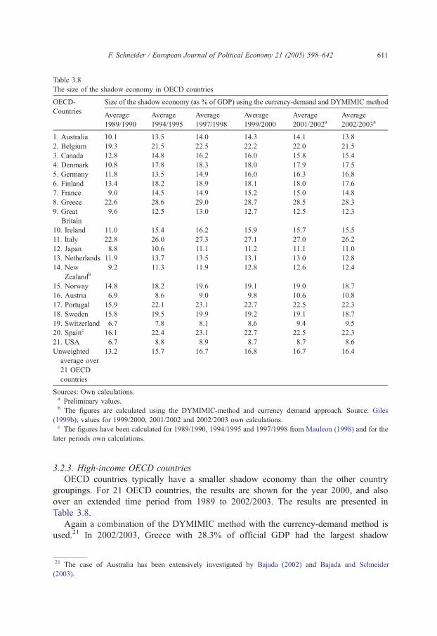
Table 3.8
The size of the shadow economy in OECD countries
OECD-
Countries
Size of the shadow economy (as % of GDP) using the currency-demand and DYMIMIC method
Average
1989/1990
Average
1994/1995
Average
1997/1998
Average
1999/2000
Average
2001/2002aAverage
2002/2003a
1. Australia 10.1 13.5 14.0 14.3 14.1 13.8
2. Belgium 19.3 21.5 22.5 22.2 22.0 21.5
3. Canada 12.8 14.8 16.2 16.0 15.8 15.4
4. Denmark 10.8 17.8 18.3 18.0 17.9 17.5
5. Germany 11.8 13.5 14.9 16.0 16.3 16.8
6. Finland 13.4 18.2 18.9 18.1 18.0 17.6
7. France 9.0 14.5 14.9 15.2 15.0 14.8
8. Greece 22.6 28.6 29.0 28.7 28.5 28.3
9. Great
Britain
9.6 12.5 13.0 12.7 12.5 12.3
10. Ireland 11.0 15.4 16.2 15.9 15.7 15.5
11. Italy 22.8 26.0 27.3 27.1 27.0 26.2
12. Japan 8.8 10.6 11.1 11.2 11.1 11.0
13. Netherlands 11.9 13.7 13.5 13.1 13.0 12.8
14. New
Zealandb9.2 11.3 11.9 12.8 12.6 12.4
15. Norway 14.8 18.2 19.6 19.1 19.0 18.7
16. Austria 6.9 8.6 9.0 9.8 10.6 10.8
17. Portugal 15.9 22.1 23.1 22.7 22.5 22.3
18. Sweden 15.8 19.5 19.9 19.2 19.1 18.7
19. Switzerland 6.7 7.8 8.1 8.6 9.4 9.5
20. Spainc 16.1 22.4 23.1 22.7 22.5 22.3
21. USA 6.7 8.8 8.9 8.7 8.7 8.6
Unweighted
average over
21 OECD
countries
13.2 15.7 16.7 16.8 16.7 16.4
Sources: Own calculations.a Preliminary values.b The figures are calculated using the DYMIMIC-method and currency demand approach. Source: Giles
(1999b); values for 1999/2000, 2001/2002 and 2002/2003 own calculations.c The figures have been calculated for 1989/1990, 1994/1995 and 1997/1998 from Mauleon (1998) and for the
later periods own calculations.
F. Schneider / European Journal of Political Economy 21 (2005) 598–642 611
3.2.3. High-income OECD countries
OECD countries typically have a smaller shadow economy than the other country
groupings. For 21 OECD countries, the results are shown for the year 2000, and also
over an extended time period from 1989 to 2002/2003. The results are presented in
Table 3.8.
Again a combination of the DYMIMIC method with the currency-demand method is
used.21 In 2002/2003, Greece with 28.3% of official GDP had the largest shadow
21 The case of Australia has been extensively investigated by Bajada (2002) and Bajada and Schneider
(2003).
F. Schneider / European Journal of Political Economy 21 (2005) 598–642612
economy, followed by Italy with 26.2%22 and Portugal with 22.3%. In the middle range
was Germany with a shadow economy of 16.8% of official GDP, followed by Ireland with
15.5% and France with 14.8% of official GDP. At the lower end were Austria with 10.8%
of GDP and the United States with 8.6% of official GDP. There was a remarkable increase
in the size of the shadow economies during the 1990s. On average the shadow economy
was 13.2% for the 21 OECD countries in 1989/1990, and 16.4% 2002/2003. In the second
half of the 1990s, the majority of OECD countries did not have increasing shadow
economies. In Belgium there was a decrease from 22.5% in 1997/1998 to 21.5% in 2002/
2003. Denmark decreased from 18.3% in 1997/1998 to 17.5% in 2002/2003 and Finland
from 18.9% to 17.6%. Italy decreased from 27.3% in 1997/1998) to 26.2% in 2002/2003.
Austria increased from 9.0% in 1997/1998 to 10.8% in 2002/2003, and Germany from
14.9% in 1997/1998 to 16.8% in 2002/2003. There is no general conclusion about whether
the shadow economy in the high-income countries was increasing or decreasing at the end
of the 1990s.
4. Dynamic effects on the official economy
4.1. Theoretical background
Generally, the informal sector or shadow economy is expected to influence the tax
system and its structure, the efficiency of resource allocation between sectors, and the
official economy in a dynamic sense. In order to study the effects of the shadow economy
on the official economy, several studies integrate underground economies into theoretical
or empirical macroeconomic models.23 For example, Houston (1987) develops a
theoretical business cycle model in which there are tax and monetary policy linkages
with the shadow economy, and concludes that the existence of a shadow economy could
lead to an overstatement of the inflationary effects of fiscal or monetary stimulus. In an
empirical study for Belgium, Adam and Ginsburgh (1985) focus on the implications of the
shadow economy on bofficialQ growth and find a positive relationship between the growth
of the shadow economy and the bofficialQ economy under certain assumptions (very low
entry costs into the shadow economy due to a low probability of enforcement). They
conclude that an expansionary fiscal policy is a positive stimulus for both the formal and
informal economies.
Another hypothesis is that a substantial reduction in size of the shadow economy leads
to a significant increase in tax revenues and therefore to a greater quantity and quality of
public goods and services, which stimulates economic growth. Some authors have found
empirical evidence for this hypothesis. Loayza (1996) presents a simple macroeconomic
endogenous growth model in which the production technology depends on congestible
public services and in which bexcessiveQ taxes and regulation are imposed by governments
23 For Austria this was done by Schneider et al. (1989) and Neck et al. (1989). For further discussion of this
aspect, see Quirk (1996) and Giles (1999a).
22 For an extensive study of the size of the shadow economy of Italy, see Del’Anno (2003) and Del’Anno and
Schneider (2004), who estimated a similar but somewhat lower magnitude for the Italian shadow economy.
F. Schneider / European Journal of Political Economy 21 (2005) 598–642 613
unable to enforce fully compliance. He concludes that an increase in the relative size of the
informal economy reduces economic growth in economies where (1) the statutory tax
burden is larger than the optimal tax burden and where (2) enforcement of compliance is
weak. The reason is the strongly negative correlation between the informal sector and
public infrastructure indices, while public infrastructure is the key element for economic
growth. Loayza (1996) also found empirical evidence for Latin America countries
indicating that if the shadow economy increases by 1 percentage point of GDP—ceteris
paribus—the growth rate of official real GDP per capita decreases by 1.22 percentage
points. However, this negative impact of informal sector activities on economic growth is
not broadly accepted. For example, see Asea (1996). Loayza (1996) set out a model based
on the assumption that the production technology depends on tax-financed public services
that are subject to congestion and that the informal sector does not pay taxes but must pay
penalties that are not used to finance public services. The negative correlation between the
size of the informal sector and economic growth is therefore not very surprising.
Further, in the neoclassical view the underground economy is desirable in the sense that
it responds to the economic environment’s demand for urban services and small-scale
manufacturing. From this point of view, the informal sector provides the economy with
dynamic entrepreneurial spirit and can lead to greater competition, higher efficiency, and
stronger boundaries and limits for government activities. The informal sector may help to
create markets, increase financial resources, enhance entrepreneurship, and transform the
legal, social, and economic institutions necessary for accumulation (Asea, 1996, p. 166).
The voluntary self-selection between the formal and informal sectors may provide a higher
potential for economic growth and underlie a positive relation between an increase of the
informal sector and economic growth.
Considering both lines of theoretical argument, the effects of an increase in the size of
the shadow economy on bofficialQ economic growth are ambiguous. It may be that on the
one hand in high-income countries people/entrepreneurs are overburdened by taxes and
regulation so that an increasing shadow economy stimulates the official economy as
additional value-added is created and the additional income earned in the shadow economy
is spent in the official economy. On the other hand, in low-income countries an increasing
shadow economy erodes the tax base, with the consequence of a lower provision of public
infrastructure and basic public services (for example an effective juridical system), with
the final consequence of lower official growth.
Giles (1997a,b, 1999a) and Giles et al. (2002) investigated the relationship between the
shadow and official economies for New Zealand and Canada, and found clear evidence of
Granger causality from official GDP to the shadow economy and only very mild evidence
of Granger causality in the reverse direction. This is supported by similar evidence for
New Zealand reported by Giles.
For the estimates undertaken here, I construct a panel data set for 110 countries for the
time period from 1990 to 2000 in order to estimate the possible effects of the shadow
economy on the official one. The panel data set consists of variables24 that growth theory
suggests are relevant for economic growth (Barro and Sala-i-Martin, 1995; Breton, 2001).
The data set includes as explanatory variables the size of the shadow economy (as a
24 A description of the countries, variables and sources can be found more detailed in Appendix A.
F. Schneider / European Journal of Political Economy 21 (2005) 598–642614
percentage of bofficialQ GDP), capital accumulation, labor force and population growth
rates, inflation rates, an indicator for openness, data on foreign direct investment, the
corruption index, government expenditures and GDP per capita (to control for the
convergence hypothesis).25
4.2. The main results
A basic equation was estimated for the entire sample of 110 developing and developed
countries, with further estimates for two separate sub-samples of 21 OECD countries and
89 developing and transition countries. Such a splitting of the total sample is an additional
test of robustness of the findings from the total sample. In all three regressions, the
dependent variable is the average growth rate of per capita GDP over the 1990–2000
period. Appendix B contains a description of the countries and variables.
4.2.1. The sample of 110 low- and high-income countries
The equation estimated is the following:
bofficialQ economic growth=a1 (shadow economy industrialized26 countries)+a2
(shadow economy developing countries)+a3 (openness)+a4 (inflation rate all other
countries)+a5 (inflation rate transition countries)+a6 (government consumption)+a7
(lagged GDP per capita growth rate)+a8 (total population)+a9 (capital accumulation
rate)+a10(constant)+eit, with the expected signs=a1N0, a2b0, a3N0, a4b0, a5b0, a6b0,
a7N0, a8N0, a9N0.
Not all of the theoretically relevant variables for economic growth were available27 for
all 110 countries (expenditures on research and development or indicators for human
capital such as school enrollment and number of persons with secondary and tertiary
education). A reduced dataset for 104 countries was used.28 Putting all possible (for all
countries available) variables into a growth equation did not deliver satisfactory results,
since many conventionally important variables were insignificant. For example, labor
force growth had no influence on the GDP growth rate in the model despite the fact that
theory suggests a positive relationship between labor force growth and economic growth
(Breton, 2001); similarly, foreign direct investment did not a statistically significant impact
on annual GDP growth. Accordingly, I followed a btesting down procedureQ29 to address
possible misspecification. The model reported in Table 4.1 is bmy bestQ model.
26 These are here the 23 transition countries and the 21 highly developed OECD countries of western type.
25 Convergence theory proposes that countries with a lower GDP per capita should have higher annual GDP
growth rates.
27 Some variables were not available at all but most variables were available only for a small number of
countries and many observations would have been lost if using the particular variable in the regression analysis
[for example using patents per year as a proxy variable for expenditures on R&D results in a sample consisting
only of 30 countries]. The 110 countries are listed in Appendix B (part 6.2).28 Unfortunately, six developing countries were lost due to missing or unreliable data.29 The dtesting down procedureT means that step by step insignificant variables are dropped from the equation
after carrying out F-tests on joint significance (see Wooldridge, 2000, pp.139–150). For example, the coefficient
on GDP per capita was insignificant and the convergence theory cannot be supported with the available data.
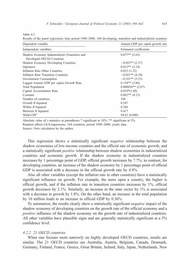
Table 4.1
Results of the panel regression; time period 1990–2000, 104 developing, transition and industrialized countries
Dependent variable Annual GDP per capita growth rate
Independent variables: Estimated coefficients:
Shadow Economy Industrialized (Transition and
Developed OECD) Countries
0.077** (2.63)
Shadow Economy Developing Countries �0.052** (2.37)
Openness 0.012** (2.14)
Inflation Rate Other Countries 0.023 (1.32)
Inflation Rate Transition Countries �0.021** (4.10)
Government Consumption �0.181** (3.23)
Lagged Annual GDP per capita Growth Rate 0.154** (3.06)
Total Population 0.000036** (2.07)
Capital Accumulation Rate 0.019*(1.88)
Constant 0.062** (4.13)
Number of countries 104
Overall R-Squared 0.347
Within R-Squared 0.266
Between R-Squared 0.417
Wald-CHI2 94.63 (0.000)
Absolute value of z-statistics in parentheses * significant at 10%; ** significant at 5%.
Random effects GLS-regressions; 104 countries, period 1990–2000; yearly data.
Source: Own calculation by the author.
F. Schneider / European Journal of Political Economy 21 (2005) 598–642 615
This regression shows a statistically significant negative relationship between the
shadow economies of low-income countries and the official rate of economic growth, and
a statistically significant positive relationship between shadow economies in industrialized
countries and economic growth. If the shadow economy in industrialized countries
increases by 1 percentage point of GDP, official growth increases by 7.7%; in contrast, for
developing countries, an increase of the shadow economy by 1 percentage point of official
GDP is associated with a decrease in the official growth rate by 4.9%.
Also all other variables (except the inflation rate in other countries) have a statistically
significant influence on growth. For example, the more open a country, the higher is
official growth, and if the inflation rate in transition countries increases by 1%, official
growth decreases by 2.1%. Similarly, an increase in the state sector by 1% is associated
with a decrease in growth by 1.8%. On the other hand, an increase in the total population
by 10 million leads to an increase in official GDP by 0.36%.
To summarize, the results clearly show a statistically significant negative impact of the
shadow economy of developing countries on the growth rate of the official economy and a
positive influence of the shadow economy on the growth rate of industrialized countries.
All other variables have plausible signs and are generally statistically significant at a 5%
confidence level.
4.2.2. 21 OECD countries
When one focuses more narrowly on highly developed OECD countries, results are
similar. The 21 OECD countries are Australia, Austria, Belgium, Canada, Denmark,
Germany, Finland, France, Greece, Great Britain, Ireland, Italy, Japan, Netherlands, New
F. Schneider / European Journal of Political Economy 21 (2005) 598–642616
Zealand, Norway, Portugal, Sweden, Switzerland, Spain, and the USA. As before, I
estimated a panel regression with the official growth rate of GDP per capita of the 1990 up
to 2000 period as dependent variable. The following growth equation was specified:
bofficialQ growth (annual GDP per capita)=a1 (trendvariable)+a2 (shadow econo-
my)+a3 (openness)+a4 (capital accumulation rate)+a5 (annual FDY growth rate)+a6
(annual labour force growth rate)+a7 (constant)+eit. For the signs we expect a1N0, a2N0,
a3N0, a4N0, a5N0.
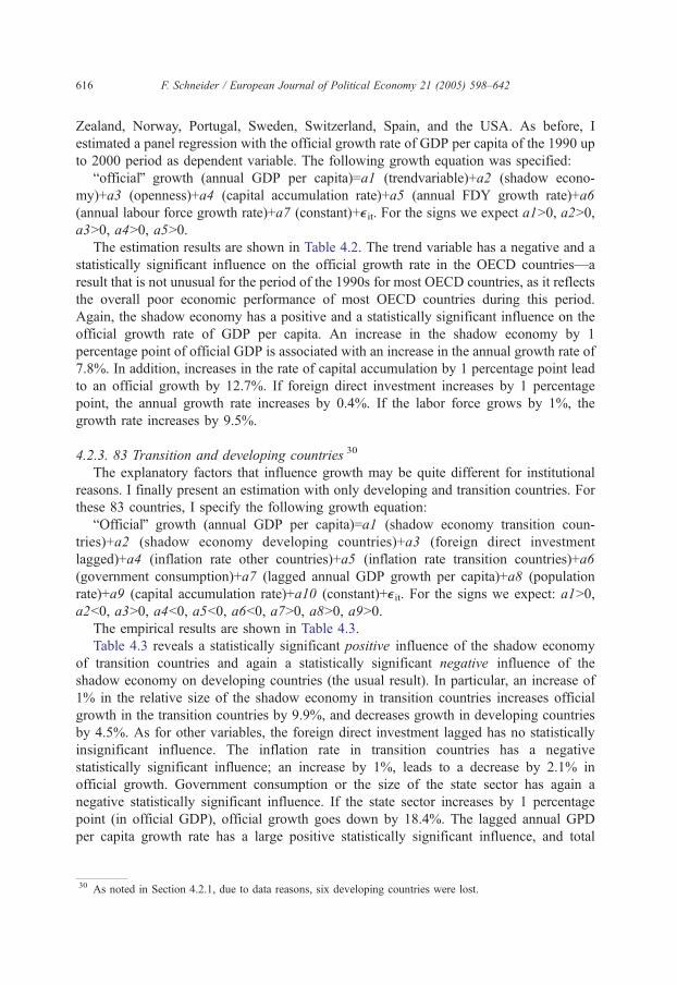
The estimation results are shown in Table 4.2. The trend variable has a negative and a
statistically significant influence on the official growth rate in the OECD countries—a
result that is not unusual for the period of the 1990s for most OECD countries, as it reflects
the overall poor economic performance of most OECD countries during this period.
Again, the shadow economy has a positive and a statistically significant influence on the
official growth rate of GDP per capita. An increase in the shadow economy by 1
percentage point of official GDP is associated with an increase in the annual growth rate of
7.8%. In addition, increases in the rate of capital accumulation by 1 percentage point lead
to an official growth by 12.7%. If foreign direct investment increases by 1 percentage
point, the annual growth rate increases by 0.4%. If the labor force grows by 1%, the
growth rate increases by 9.5%.
4.2.3. 83 Transition and developing countries 30
The explanatory factors that influence growth may be quite different for institutional
reasons. I finally present an estimation with only developing and transition countries. For
these 83 countries, I specify the following growth equation:
bOfficialQ growth (annual GDP per capita)=a1 (shadow economy transition coun-
tries)+a2 (shadow economy developing countries)+a3 (foreign direct investment
lagged)+a4 (inflation rate other countries)+a5 (inflation rate transition countries)+a6
(government consumption)+a7 (lagged annual GDP growth per capita)+a8 (population
rate)+a9 (capital accumulation rate)+a10 (constant)+eit. For the signs we expect: a1N0,
a2b0, a3N0, a4b0, a5b0, a6b0, a7N0, a8N0, a9N0.
The empirical results are shown in Table 4.3.
Table 4.3 reveals a statistically significant positive influence of the shadow economy
of transition countries and again a statistically significant negative influence of the
shadow economy on developing countries (the usual result). In particular, an increase of
1% in the relative size of the shadow economy in transition countries increases official
growth in the transition countries by 9.9%, and decreases growth in developing countries
by 4.5%. As for other variables, the foreign direct investment lagged has no statistically
insignificant influence. The inflation rate in transition countries has a negative
statistically significant influence; an increase by 1%, leads to a decrease by 2.1% in
official growth. Government consumption or the size of the state sector has again a
negative statistically significant influence. If the state sector increases by 1 percentage
point (in official GDP), official growth goes down by 18.4%. The lagged annual GPD
per capita growth rate has a large positive statistically significant influence, and total
30 As noted in Section 4.2.1, due to data reasons, six developing countries were lost.
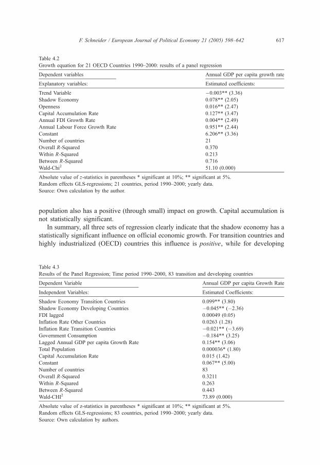
Table 4.2
Growth equation for 21 OECD Countries 1990–2000: results of a panel regression
Dependent variables Annual GDP per capita growth rate
Explanatory variables: Estimated coefficients:
Trend Variable �0.003** (3.36)
Shadow Economy 0.078** (2.05)
Openness 0.016** (2.47)
Capital Accumulation Rate 0.127** (3.47)
Annual FDI Growth Rate 0.004** (2.49)
Annual Labour Force Growth Rate 0.951** (2.44)
Constant 6.206** (3.36)
Number of countries 21
Overall R-Squared 0.370
Within R-Squared 0.213
Between R-Squared 0.716
Wald-Chi2 51.10 (0.000)
Absolute value of z-statistics in parentheses * significant at 10%; ** significant at 5%.
Random effects GLS-regressions; 21 countries, period 1990–2000; yearly data.
Source: Own calculation by the author.
F. Schneider / European Journal of Political Economy 21 (2005) 598–642 617
population also has a positive (through small) impact on growth. Capital accumulation is
not statistically significant.
In summary, all three sets of regression clearly indicate that the shadow economy has a
statistically significant influence on official economic growth. For transition countries and
highly industrialized (OECD) countries this influence is positive, while for developing
Table 4.3
Results of the Panel Regression; Time period 1990–2000, 83 transition and developing countries
Dependent Variable Annual GDP per capita Growth Rate
Independent Variables: Estimated Coefficients:
Shadow Economy Transition Countries 0.099** (3.80)
Shadow Economy Developing Countries �0.045** (�2.36)
FDI lagged 0.00049 (0.05)
Inflation Rate Other Countries 0.0263 (1.28)
Inflation Rate Transition Countries �0.021** (�3.69)
Government Consumption �0.184** (3.25)
Lagged Annual GDP per capita Growth Rate 0.154** (3.06)
Total Population 0.000036* (1.80)
Capital Accumulation Rate 0.015 (1.42)
Constant 0.067** (5.00)
Number of countries 83
Overall R-Squared 0.3211
Within R-Squared 0.263
Between R-Squared 0.443
Wald-CHI2 73.89 (0.000)
Absolute value of z-statistics in parentheses * significant at 10%; ** significant at 5%.
Random effects GLS-regressions; 83 countries, period 1990–2000; yearly data.
Source: Own calculation by authors.
Table 5.1
Average size of the shadow economy for developing, transition and OECD-countries in terms of value-added for
2000
Countries/Year Average Size of the Shadow Economy-Value added in % of official GDP
using DYMIMIC and Currency Demand method
(Number of Countries)
Mostly developing countries: 1990/91 1994/95 1999/2000
Africa 33.9 (24) 37.4 (24) 41.2 (24)
Central and South America 34.2 (17) 37.7 (17) 41.5 (17)
Asia 20.9 (25) 23.4 (25) 26.3 (25)
Transition countries 31.5 (23) 34.6 (23) 37.9 (23)
Highly developed
OECD Countries
13.2 (21) 15.7 (21) 16.8 (21)
Source: Own calculations.
F. Schneider / European Journal of Political Economy 21 (2005) 598–642618
countries the shadow economy has a negative influence on official growth. These results
(at least partly) confirm the discussion of the theoretical considerations in part 5.1.
5. Summary and conclusions
There are many obstacles to overcome in measuring the size of the shadow economy
and in analyzing consequences for the official economy, but progress has been made. I
have provided estimates of the size of the shadow economies for 110 countries for three
periods of time (1990/1991, 1994/1995 and 1999/2000) using the DYMIMIC and the
currency demand approach, allowing insights can be provided into the size and
development of the shadow economy of developing, transition and highly developed
OECD countries.31 The first conclusion from these results is that for all countries
investigated the shadow economy has reached a remarkably large size; the summarized
results are shown in Table 5.1.
Moreover, I have also demonstrated empirically strong interaction of the shadow
economy with government policies and with the official economy. From these empirical
results I draw three further conclusions:
(1) The empirical results convincingly demonstrate that an increasing burden of taxation
and social security payments, combined with rising state regulatory activities, are the
major driving forces underlying the size and growth of the shadow economy.
(2) A further important result is that the shadow economy has a statistically significant
and quantitatively important influence on the growth of the official economy. If the
shadow economy increases by one percentage point (shadow economy in percent of
official GDP) the official growth in a developing country declines between 4.5% and
5.7%. For developed (industrialized and/or transition) countries we find the opposite
31 The appendix provides critical discussion of these two methods, which have well known weaknesses,
compare also Pedersen (2003).
F. Schneider / European Journal of Political Economy 21 (2005) 598–642 619
result. If the shadow economy increases by one percentage point (in % of GDP) the
growth rate in industrialized countries increases by 7.7% and by 9.9% in transition
countries, respectively.
(3) Finally, to conclude: Shadow economies are a complex phenomenon, present to a
significant extent in all type of economies (developing, transition and developed).
People engage in shadow economic activity for a variety of reasons, among most
important of which are government actions, most notable taxation and regulation.
These two insights are accompanied by a third, no less important one: a government
aiming to decrease shadow economic activity has first and foremost to analyze the
complex relationships between the official and shadow economies—and even more
important—consequences of its own policy decisions.
Acknowledgements
I thank an anonymous referee for most helpful and stimulating comments. I am also
indebted to Robert Klinglmair for his help of the compiling of the data and the
econometric investigations of an earlier version of this paper.
Appendix A. Methods to estimate the size of the shadow economy
As noted, estimating the size of a shadow economy is a difficult and challenging task.
In this Appendix I give a short but comprehensive overview on the various procedures for
estimating the size of a shadow economy. Three different types of methods are most
widely used, and each is briefly discussed.
A.1. Direct approaches
These are micro approaches that employ either well designed surveys and samples
based on voluntary replies or tax auditing and other compliance methods. Sample surveys
designed to estimate the shadow economy are widely used in a number of countries.32 The
main disadvantages of this method are the flaws of all surveys. For example, the average
precision and results depend greatly on the respondent’s willingness to cooperate, it is
difficult to asses the amount of undeclared work from a direct questionnaire, most
interviewers hesitate to confess to fraudulent behavior, and responses are of uncertain
reliability, which makes it difficult to calculate a true estimate (in monetary terms) of the
extend of undeclared work. The main advantage of this method lies in the detailed
32 The direct method of voluntary sample surveys has been extensively used for Norway by Isachsen et al.
(1982), and Isachsen and Strom (1985). For Denmark this method is used by Mogensen et al. (1995) in which
they report estimatesb of the shadow economy of 2.7% of GDP for 1989, of 4.2% of GDP for 1991, of 3.0% of
GDP for 1993 and of 3.1% of GDP for 1994. In Pedersen (2003) estimates of the Danish shadow economy
contain the years 1995 with 3.1% up to 2001 with 3.8%.
F. Schneider / European Journal of Political Economy 21 (2005) 598–642620
information about the structure of the shadow economy but the results from these kinds of
surveys are very sensitive to the way the questionnaire is formulated.33
Estimates of the shadow economy can also be based on the discrepancy between
income declared for tax purposes and that measured by selective checks. Fiscal auditing
programs have been particularly effective in this regard. Since these programs are designed
to measure the amount of undeclared taxable income, they may also be used to calculate
the size of the shadow economy.34 However, a number of difficulties beset this approach.
First, using tax compliance data is equivalent to using a (possibly biased) sample of the
population. In general, the selection of taxpayers for tax audits is not random but based on
properties of submitted (tax) returns that indicate a certain likelihood of tax fraud.
Consequently, such a sample is not a random one of the whole population and estimates of
the shadow based upon a biased sample may not be accurate. Second, estimates based on
tax audits reflect only that portion of shadow economy income that the authorities succeed
in discovering, and this is likely to be only a fraction of hidden income.
A further disadvantage of these two direct methods (surveys and tax auditing) is that
they lead only to point estimates. It is unlikely that they capture all shadow activities, so
they can be seen as providing lower bound estimates. They are unable to provide estimates
of the development and growth of the shadow economy over a longer period of time. As
already noted, they have however at least one considerable advantage—they can provide
detailed information about shadow economy activities and the structure and composition
of those who work in the shadow economy.
A.2. Indirect approaches
These approaches, which are also called indicator approaches, are mostly macro-
economic and use various economic and other indicators that contain information about
the development of the shadow economy (over time). Currently there are five indicators
that leave some traces of the shadow economy.
A.2.1. The discrepancy between national expenditure and income statistics
This approach is based on discrepancies between income and expenditure statistics. In
national accounting the income measure of GNP should be equal to the expenditure
measure of GNP. Thus, if an independent estimate of the expenditure site of the national
accounts is available, the gap between the expenditure measure and the income measure
can be used as an indicator of the extent of the black economy.35 Since national accounts
statisticians are anxious to minimize this discrepancy, the initial discrepancy or first
estimate, rather than the published discrepancy, should be employed as an estimate of the
shadow economy. If all the components of the expenditure side are measured without
33 The advantages and disadvantages of this method are extensively dealt by Pedersen (2003) and Mogensen et
al. (1995) in their excellent and very carefully done investigations.34 In the United States, IRS (1979, 1983), Simon and Witte (1982), Witte (1987), Clotefelter (1983), and Feige
(1986). For a more detailed discussion, see Dallago (1990) and Thomas (1992).35 See, e.g., Franz (1983) for Austria; MacAfee (1980), O’Higgins (1989) and Smith (1985), for Great Britain;
Petersen (1982) and Del Boca (1981) for Germany; Park (1979) for the United States. For a critical survey, see
Thomas (1992).
F. Schneider / European Journal of Political Economy 21 (2005) 598–642 621
error, then this approach would indeed yield a good estimate of the scale of the shadow
economy. Unfortunately, however, this is not the case. Instead, the discrepancy reflects all
omissions and errors everywhere in the national accounts statistics as well as shadow
economy activity. These estimates may therefore be very crude and of questionable
reliability.36
A.2.2. The discrepancy between the official and actual labor force
A decline in participation of the labor force in the official economy can be seen as an
indication of increased activity in the shadow economy. If total labor force participation is
assumed to be constant, than a decreasing official rate of participation can be seen as an
indicator of an increase in the activities in the shadow economy, ceteris paribus.37 One
weakness of this method is that differences in the rate of participation may also have other
causes. Also, people can work in the shadow economy and have a job in the official
economy. Therefore such estimates may be viewed as weak indicators of the size and
development of the shadow economy.
A.2.3. The transactions approach
This approach has been most fully developed by Feige.38 It is based upon the
assumption that there is a constant relation over time between the volume of transaction
and official GNP, as summarized by the well-known Fisherian quantity equation, or
M*V=p*T (with M money, V velocity, p prices, and T total transactions). Assumptions
also have to be made about the velocity of money and about the relationships between the
value of total transactions p*T and total (official+unofficial) nominal GNP. Relating total
nominal GNP to total transactions, the GNP of the shadow economy can be calculated by
subtracting the official GNP from total nominal GNP. However, to derive figures for the
shadow economy, one must also assume a base year in which there is no shadow economy
and therefore the ratio of p*T to total nominal (official=total) GNP was bnormalQ andwould have been constant over time if there had been no shadow economy. To obtain
reliable shadow economy estimates, precise figures of the total volume of transactions are
required, which might be especially difficult for cash transactions, which depend, among
other factors, on the durability of bank notes through the quality of the paper on which the
notes are printed.39 Also, the assumption is made that all variations in the ratio between the
total value of transaction and the officially measured GNP are due to the shadow economy.
This means that a considerable amount of data is required in order to eliminate financial
transactions from bpureQ cross payments, which are legal and have nothing to do with the
shadow economy. In general, although this approach is theoretically attractive, the
36 A related approach is pursued by Pissarides and Weber (1988), who use micro data from household budget
surveys to estimate the extent of income understatement by self-employed.37 Such studies have been made for Italy, see e.g., Contini (1981) and Del Boca (1981); for the United States, see
O’Neill (1983), for a critical survey, see again Thomas (1992).38 For an extended description of this approach, see Feige (1996); for a further application for the Netherlands,
Boeschoten and Fase (1984), and for Germany, Langfeldt (1984).39 For a detailed criticism of the transaction approach, see Boeschoten and Fase (1984), Frey and Pommerehne
(1984), Kirchgassner (1984), Tanzi (1982a,b, 1986), Dallago (1990), Thomas (1986, 1992, 1999) and Giles
(1999a).
F. Schneider / European Journal of Political Economy 21 (2005) 598–642622
empirical requirements necessary to obtain reliable estimates are so difficult to fulfill that
its application may lead to doubtful results.
A.2.4. The currency demand approach
The currency demand approach was first used by Cagan (1958), who considered the
correlation between currency demand and tax pressure (as one cause of the shadow
economy) for the United States over the period 1919–1955. Twenty years later, Gutmann
(1977) used the same approach but without any statistical procedures. Cagan’s approach
was further developed by Tanzi (1980, 1983), who estimated a currency demand function
for the United States for the period 1929 to 1980 in order to calculate the size of the
shadow economy. His approach assumes that shadow (or hidden) transactions are
undertaken in the form of cash payments, so as to leave no observable traces for the
authorities. An increase in the size of the shadow economy will therefore increase the
demand for currency. To isolate the resulting excess demand for currency, an equation for
currency demand is estimated over time. All conventional possible factors, such as the
development of income, payment habits, interest rates, and so on, are controlled for.
Additionally, such variables as the direct and indirect tax burden, government regulation
and the complexity of the tax system, which are assumed to be the major factors causing
people to work in the shadow economy, are included in the estimation equation. The basic
regression equation for the currency demand, proposed by Tanzi (1983), is the following:
ln C=M2Þt ¼ bO þ b1ln 1þ TWð Þt þ b2ln WS=Yð Þt þ b3ln Rt þ b4ln Y=Nð Þt þ ut�
with b1N0, b2N0, b3b0, b4N0 where ln denotes natural logarithms, C/M2 is the ratio of
cash holdings to current and deposit accounts, TW is a weighted average tax rate (to proxy
changes in the size of the shadow economy), WS/Y is a proportion of wages and salaries in
national income (to capture changing payment and money holding patterns), R is the
interest paid on savings deposits (to capture the opportunity cost of holding cash) and Y/N
is the per capita income.40 Any bexcessQ increase in currency, or the amount unexplained
by the conventional or normal factors is then attributed to the rising tax burden and the
other reasons leading people to work in the shadow economy. Figures for the size and
development of the shadow economy can be calculated in a first step by comparing the
difference between the development of currency when the direct and indirect tax burden
and government regulation are held at lowest values, and the development of currency
with the current (higher) burden of taxation and government regulation. Assuming in a
second step the same income velocity for currency used in the shadow economy as for
legal M1 in the official economy, the size of the shadow can be computed and compared to
the official GDP. This is one of the most commonly used approaches. It has been applied
to many OECD countries41 but has nevertheless been criticized on various grounds.42 The
40 The estimation of such a currency demand equation has been criticized by Thomas (1999) but part of this
criticism has been considered by the work of Giles (1999a,b) and Bhattacharyya (1999), who both use the latest
econometric techniques.41 See Karmann (1986, 1990), Schneider (1997, 1998a), Johnson et al. (1998a), and Williams and Windebank
(1995).42 See Thomas (1992, 1999), Feige (1986), Pozo (1996), Pedersen (2003) and Ahumada et al. (2004).
F. Schneider / European Journal of Political Economy 21 (2005) 598–642 623
most commonly raised objections to this method are: (1) Not all transactions in the shadow
economy are paid in cash. Isachsen and Strom (1985) used the survey method to find out
that in Norway, in 1980, roughly 80% of all transactions in the hidden sector were paid in
cash. The size of the total shadow economy (including barter) may thus be even larger than
previously estimated. (2) Most studies consider only one particular factor, the tax burden,
as a cause of the shadow economy. But others (such as the impact of regulation, taxpayers’
attitudes toward the state, tax morality and so on) are not considered, because reliable data
for most countries is not available. If, as seems likely, these other factors also have an
impact on the extent of the hidden economy, it might again be higher than reported in most
studies.43 (3) As discussed by Garcia (1978), Park (1979), and Feige (1996), increases in
currency demand deposits are due largely to a slowdown in demand deposits rather than to
an increase in currency caused by activities in the shadow economy, at least in the case of
the United States. (4) Blades (1982) and Feige (1986, 1996) criticize Tanzi’s studies on the
grounds that the US dollar is used as an international currency so that Tanzi should have
considered (and controlled for) the presence of US dollars, which are used as an
international currency and held in cash abroad.44 Frey and Pommerehne (1984) and
Thomas (1986, 1992, 1999) claim that Tanzi’s parameter estimates are not very stable.45
(5) Most studies assume the same velocity of money in official and shadow economies. As
argued by Hill and Kabir (1996) for Canada and by Klovland (1984) for the Scandinavian
countries, there is considerable uncertainty about the velocity of money in the official
economy, and the velocity of money in the hidden sector is even more difficult to estimate.
Without knowledge about the velocity of currency in the shadow economy, one has to
accept the assumption of an equal money velocity in both sectors. (6) Ahumada et al.
(2004) show that the currency approach together with the assumption of equal income
velocity of money in the reported and the hidden transaction is only correct if the income
elasticity is 1. (7) Finally, the assumption of no shadow economy in a base year is open to
criticism. Relaxing this assumption would again imply an upward adjustment of the size of
the shadow economy.
43 One (weak) justification for the only use of the tax variable is that this variable has by far the strongest impact
on the size of the shadow economy in the studies known to the authors. The only exception is the study by Frey
and Weck-Hannemann (1984) where the variable btax immoralityQ has a quantitatively larger and statistically
stronger influence than the direct tax share in the model approach. In the study of Pommerehne and Schneider
(1985) for the US, besides various tax measures, data for regulation, tax immorality, minimum wage rates are
available, the tax variable has a dominating influence and contributes roughly 60–70% to the size of the shadow
economy. See also Zilberfarb (1986).44 Another study by Tanzi (1982, esp. pp. 110–113) explicitly deals with this criticism. A very careful
investigation of the amount of US dollars used abroad and US currency used in the shadow economy and for
bclassicalQ crime activities has been undertaken by Rogoff (1998), who concludes that large denomination bills
are major driving force for the growth of the shadow economy and classical crime activities, due largely to
reduced transactions costs.45 However in studies for European countries Kirchgassner (1983, 1984) and Schneider (1986) conclude that the
estimation results for Germany, Denmark, Norway and Sweden are quite robust when using the currency demand
method. Hill and Kabir (1996) find for Canada that the rise of the shadow economy varies with respect to the tax
variable used; they conclude bwhen the theoretically best tax rates are selected and a range of plausible velocity
values is used, this method estimates underground economic growth between 1964 and 1995 at between 3% and
11% of GDP.Q (p. 1553).
F. Schneider / European Journal of Political Economy 21 (2005) 598–642624
A.2.5. The physical input (electricity consumption) method
A.2.5.1. The Kaufmann-Kaliberda Method 46. To measure overall (official and
unofficial) economic activity in an economy, Kaufmann and Kaliberda (1996) assume
that electric-power consumption is regarded as the single best physical indicator of overall
(or official plus unofficial) economic activity. Overall economic activity and electricity
consumption have been empirically observed throughout the world to move in lockstep
with electricity to GDP elasticity usually close to one. This means that the growth of total
electricity consumption is an indicator for growth of overall (official and unofficial) GDP.
By having this proxy measurement for the overall economy and then subtracting from this
overall measure the estimates of official GDP, Kaufmann and Kaliberda (1996) derive an
estimate of unofficial GDP. This method is very simple and appealing. However, it can
also be criticized on various grounds: (1) Not all shadow economy activities require a
considerable amount of electricity (e.g. personal services), and other energy sources can be
used (gas, oil, coal, etc.). Only a part of the shadow economy will be indicated. (2) Over
time, there has been considerable technical progress so that both the production and use of
electricity are more efficient than in the past, and this will apply in both official and
unofficial uses. (3) There may be considerable differences or changes in the elasticity of
electricity/GDP across countries and over time.47
A.2.5.2. The Lacko method. Lacko (1996, 1998, 1999, 2000) assumes that a certain part
of the shadow economy is associated with the household consumption of electricity. This
part comprises the so-called household production, do-it-yourself activities, and other non-
registered production and services. Lacko further assumes that in countries where the
portion of the shadow economy associated with the household electricity consumption is
high, the rest of the hidden economy (or the part Lacko cannot measure) will also be high.
Lacko (1996, pp. 19 ff.) assumes that in each country a part of the household consumption
of electricity is used in the shadow economy. Lacko’s approach (1998, p. 133) can be
described by the following two equations:
ln Ei=a1 ln Ci+a2 ln PRi+a3 Gi+a4 Qi+a5 Hi+ui , with a1N0, a2b0, a3N0, a4b0, a5N0and Hi=b1 Ti+b2 (Si�Ti)+b3 Di with b1N0, b2b0, b3N0 where i indicates the number
assigned to the country, Ei is per capita household electricity consumption in country i, Ci
is per capita real consumption of households without the consumption of electricity in
country i in US dollars (at purchasing power parity), PRi is the real price of consumption
of 1 kW h of residential electricity in US dollars (at purchasing power parity), Gi is the
relative frequency of months with the need of heating in houses in country i, Qi is the ratio
of energy sources other than electricity energy to all energy sources in household energy
consumption, Hi is the per capita output of the hidden economy, and Ti is the ratio of the
sum of paid personal income, corporate profit and taxes on goods and services to GDP, Siis the ratio of public social welfare expenditures to GDP, and Di is the sum on number of
dependants over 14 years and of inactive earners, both per 100 active earners. In a cross-
46 This method was used earlier by Lizzeri (1979), Del Boca and Forte (1982), and then was used much later by
Portes (1996), Kaufmann and Kaliberda (1996), Johnson et al. (1997). For a critique see Lacko (1998).47 Johnson et al. (1997) make an attempt to adjust for changes in the elasticity of electricity/GDP.
F. Schneider / European Journal of Political Economy 21 (2005) 598–642 625
country study, she estimates the first equation substituting for Hi with the second equation.
For the calculation of the actual size (value added) of the shadow economy, Lacko further
must know how much GDP is produced by one unit of electricity in the shadow economy
of each country. Since these data are not known, she takes the result of one of the known
shadow economy estimates that were carried out for a market economy with another
approach for the early 1990s, and applies this to the other countries. Lacko used the
shadow economy of the United States as such a base (the shadow economy value of 10.5%
of GDP taken from Morris, 1993), and then she calculates the size of the shadow economy
for other countries. Lacko’s method is also open to criticism: (1) Not all shadow economy
activities require a considerable amount of electricity and other energy sources can be
used. (2) Shadow economy activities do not take place only in the household sector. (3) It
is doubtful whether the ratio of social welfare expenditures can be used as the explanatory
factor for the shadow economy, especially in transition and developing countries. It is
questionable which is the most reliable base value of the shadow economy for calculating
the size of the shadow economy for all other countries, especially for transition and
developing countries.
A.2.6. The model approach 48
All methods described so far consider just one indicator that to capture all effects of
the shadow economy. However, shadow economy effects show up simultaneously in the
production, labor, and money markets. An even more important critique is that the
causes that determine the size of the shadow economy are taken into account only in
some of the monetary approach studies that usually consider one cause, the burden of
taxation. The model approach explicitly considers multiple causes of the existence and
growth of the shadow economy, as well as the multiple effects of the shadow economy
over time. The empirical method used is quite different from those used so far. It is
based on the statistical theory of unobserved variables, which considers multiple causes
and multiple indicators of the phenomenon to be measured. For the estimation, a factor-
analytic approach is used to measure the hidden economy as an unobserved variable over
time. The unknown coefficients are estimated in a set of structural equations within
which the bunobservedQ variable cannot be measured directly. The DYMIMIC (dynamic
multiple-indicators multiple-causes) model consists in general of two parts, with the
measurement model linking the unobserved variables to observed indicators.49 The
structural equations model specifies causal relationships among the unobserved variables.
In this case, there is one unobserved variable, or the size of the shadow economy: this is
assumed to be influenced by a set of indicators for the shadow economy’s size, thus
capturing the structural dependence of the shadow economy on variables that may be
48 This summary is derived from a longer study by Aigner et al. (1988, p. 303), applying this approach for the
United States over time; for Germany this approach has been applied by Karmann (1986, 1990). The pioneers of
this approach are Weck (1983), Frey and Weck-Hannemann (1984), who applied this approach to cross-section
data from the 24 OECD countries for various years. Before turning to this approach they developed the concept of
bsoft modelingQ (Frey et al., 1982, Frey and Weck, 1983a,b), an approach which has been used to provide a
ranking of the relative size of the shadow economy in different countries.49 One of the latest paper dealing extensively with the DYMIMIC approach, its development and its weaknesses
is from Del’Anno (2003) as well as the excellent study by Giles and Tedds (2002).
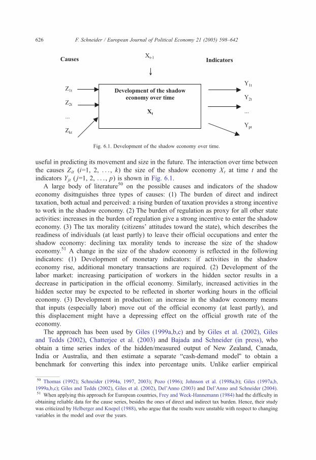
Fig. 6.1. Development of the shadow economy over time.
F. Schneider / European Journal of Political Economy 21 (2005) 598–642626
useful in predicting its movement and size in the future. The interaction over time between
the causes Zit (i=1, 2, . . . , k) the size of the shadow economy Xt at time t and the
indicators Yjt ( j=1, 2, . . . , p) is shown in Fig. 6.1.
A large body of literature50 on the possible causes and indicators of the shadow
economy disitnguishes three types of causes: (1) The burden of direct and indirect
taxation, both actual and perceived: a rising burden of taxation provides a strong incentive
to work in the shadow economy. (2) The burden of regulation as proxy for all other state
activities: increases in the burden of regulation give a strong incentive to enter the shadow
economy. (3) The tax morality (citizens’ attitudes toward the state), which describes the
readiness of individuals (at least partly) to leave their official occupations and enter the
shadow economy: declining tax morality tends to increase the size of the shadow
economy.51 A change in the size of the shadow economy is reflected in the following
indicators: (1) Development of monetary indicators: if activities in the shadow
economy rise, additional monetary transactions are required. (2) Development of the
labor market: increasing participation of workers in the hidden sector results in a
decrease in participation in the official economy. Similarly, increased activities in the
hidden sector may be expected to be reflected in shorter working hours in the official
economy. (3) Development in production: an increase in the shadow economy means
that inputs (especially labor) move out of the official economy (at least partly), and
this displacement might have a depressing effect on the official growth rate of the
economy.
The approach has been used by Giles (1999a,b,c) and by Giles et al. (2002), Giles
and Tedds (2002), Chatterjee et al. (2003) and Bajada and Schneider (in press), who
obtain a time series index of the hidden/measured output of New Zealand, Canada,
India or Australia, and then estimate a separate bcash-demand modelQ to obtain a
benchmark for converting this index into percentage units. Unlike earlier empirical
50 Thomas (1992); Schneider (1994a, 1997, 2003); Pozo (1996); Johnson et al. (1998a,b); Giles (1997a,b,
1999a,b,c); Giles and Tedds (2002), Giles et al. (2002), Del’Anno (2003) and Del’Anno and Schneider (2004).51 When applying this approach for European countries, Frey and Weck-Hannemann (1984) had the difficulty in
obtaining reliable data for the cause series, besides the ones of direct and indirect tax burden. Hence, their study
was criticized by Helberger and Knepel (1988), who argue that the results were unstable with respect to changing
variables in the model and over the years.
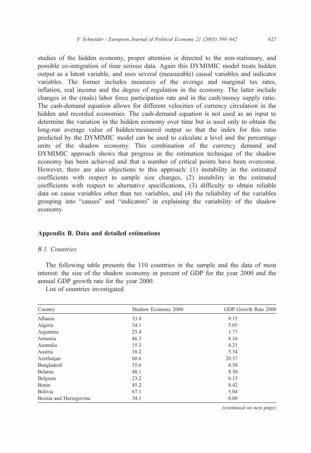
F. Schneider / European Journal of Political Economy 21 (2005) 598–642 627
studies of the hidden economy, proper attention is directed to the non-stationary, and
possible co-integration of time serious data. Again this DYMIMIC model treats hidden
output as a latent variable, and uses several (measurable) causal variables and indicator
variables. The former includes measures of the average and marginal tax rates,
inflation, real income and the degree of regulation in the economy. The latter include
changes in the (male) labor force participation rate and in the cash/money supply ratio.
The cash-demand equation allows for different velocities of currency circulation in the
hidden and recorded economies. The cash-demand equation is not used as an input to
determine the variation in the hidden economy over time but is used only to obtain the
long-run average value of hidden/measured output so that the index for this ratio
predicted by the DYMIMIC model can be used to calculate a level and the percentage
units of the shadow economy. This combination of the currency demand and
DYMIMIC approach shows that progress in the estimation technique of the shadow
economy has been achieved and that a number of critical points have been overcome.
However, there are also objections to this approach: (1) instability in the estimated
coefficients with respect to sample size changes, (2) instability in the estimated
coefficients with respect to alternative specifications, (3) difficulty to obtain reliable
data on cause variables other than tax variables, and (4) the reliability of the variables
grouping into bcausesQ and bindicatorsQ in explaining the variability of the shadow
economy.
Appendix B. Data and detailed estimations
B.1. Countries
The following table presents the 110 countries in the sample and the data of most
interest: the size of the shadow economy in percent of GDP for the year 2000 and the
annual GDP growth rate for the year 2000.
List of countries investigated
Country Shadow Economy 2000 GDP Growth Rate 2000
Albania 33.4 9.15
Algeria 34.1 5.05
Argentina 25.4 1.77
Armenia 46.3 8.16
Australia 15.3 4.21
Austria 10.2 5.34
Azerbaijan 60.6 20.37
Bangladesh 35.6 8.58
Belarus 48.1 8.30
Belgium 23.2 6.13
Benin 45.2 8.42
Bolivia 67.1 5.04
Bosnia and Herzegovina 34.1 0.00
(continued on next page)
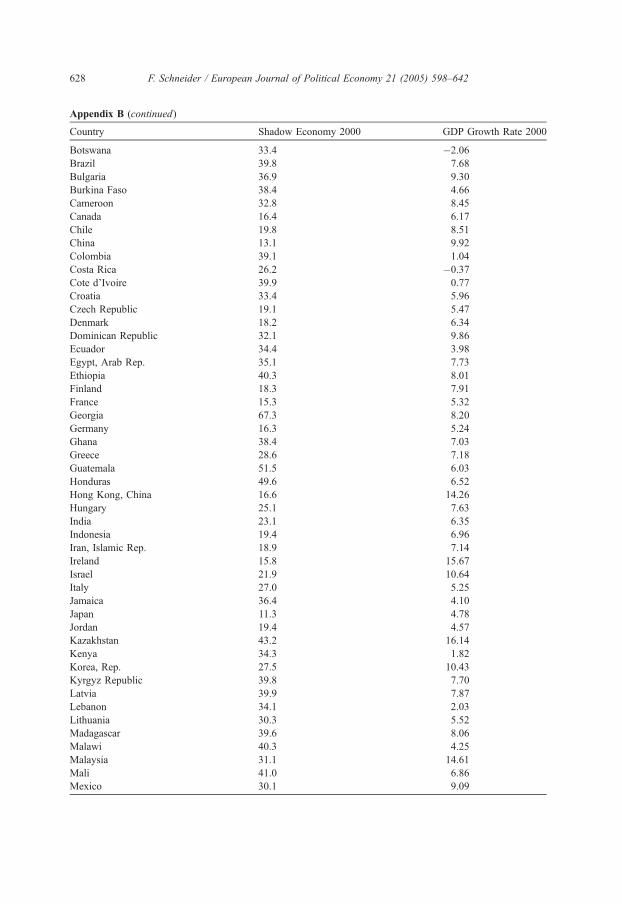
Appendix B (continued)
Country Shadow Economy 2000 GDP Growth Rate 2000
Botswana 33.4 �2.06
Brazil 39.8 7.68
Bulgaria 36.9 9.30
Burkina Faso 38.4 4.66
Cameroon 32.8 8.45
Canada 16.4 6.17
Chile 19.8 8.51
China 13.1 9.92
Colombia 39.1 1.04
Costa Rica 26.2 �0.37
Cote d’Ivoire 39.9 0.77
Croatia 33.4 5.96
Czech Republic 19.1 5.47
Denmark 18.2 6.34
Dominican Republic 32.1 9.86
Ecuador 34.4 3.98
Egypt, Arab Rep. 35.1 7.73
Ethiopia 40.3 8.01
Finland 18.3 7.91
France 15.3 5.32
Georgia 67.3 8.20
Germany 16.3 5.24
Ghana 38.4 7.03
Greece 28.6 7.18
Guatemala 51.5 6.03
Honduras 49.6 6.52
Hong Kong, China 16.6 14.26
Hungary 25.1 7.63
India 23.1 6.35
Indonesia 19.4 6.96
Iran, Islamic Rep. 18.9 7.14
Ireland 15.8 15.67
Israel 21.9 10.64
Italy 27.0 5.25
Jamaica 36.4 4.10
Japan 11.3 4.78
Jordan 19.4 4.57
Kazakhstan 43.2 16.14
Kenya 34.3 1.82
Korea, Rep. 27.5 10.43
Kyrgyz Republic 39.8 7.70
Latvia 39.9 7.87
Lebanon 34.1 2.03
Lithuania 30.3 5.52
Madagascar 39.6 8.06
Malawi 40.3 4.25
Malaysia 31.1 14.61
Mali 41.0 6.86
Mexico 30.1 9.09
F. Schneider / European Journal of Political Economy 21 (2005) 598–642628
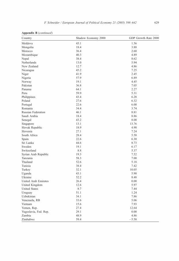
Appendix B (continued)
Country Shadow Economy 2000 GDP Growth Rate 2000
Moldova 45.1 1.56
Mongolia 18.4 3.88
Morocco 36.4 2.60
Mozambique 40.3 4.89
Nepal 38.4 8.62
Netherlands 13.0 5.94
New Zealand 12.7 4.86
Nicaragua 45.2 7.25
Niger 41.9 2.45
Nigeria 57.9 6.89
Norway 19.1 4.45
Pakistan 36.8 7.05
Panama 64.1 2.27
Peru 59.9 5.31
Philippines 43.4 6.28
Poland 27.6 6.32
Portugal 22.6 6.00
Romania 34.4 3.74
Russian Federation 46.1 8.81
Saudi Arabia 18.4 8.86
Senegal 43.2 8.08
Singapore 13.1 13.76
Slovak Republic 18.9 4.90
Slovenia 27.1 7.24
South Africa 28.4 5.58
Spain 22.6 6.30
Sri Lanka 44.6 8.73
Sweden 19.1 6.17
Switzerland 8.8 5.37
Syrian Arab Republic 19.3 7.52
Tanzania 58.3 7.00
Thailand 52.6 5.18
Tunisia 38.4 7.42
Turkey 32.1 10.05
Uganda 43.1 5.90
Ukraine 52.2 8.48
United Arab Emirates 26.4 0.00
United Kingdom 12.6 5.97
United States 8.7 7.44
Uruguay 51.1 1.24
Uzbekistan 34.1 7.86
Venezuela, RB 33.6 5.06
Vietnam 15.6 7.93
Yemen, Rep. 27.4 12.64
Yugoslavia, Fed. Rep. 29.1 0.00
Zambia 48.9 4.86
Zimbabwe 59.4 �5.58
F. Schneider / European Journal of Political Economy 21 (2005) 598–642 629
F. Schneider / European Journal of Political Economy 21 (2005) 598–642630
B.2. Definition of the variables
(1) All calculations and estimations are based on the software package dIntercooledStata 8.0T.
(2) All growth rates or shares as described in the following section. For example a
growth rate of 2% is defined as 0.02 instead of 2.0.
(3) If for some reasons observations for important countries for 1 year are missing we
used the following formula to calculate the average growth rate for these variables:
variabletþn
variablet
� �1=n
¼ F growth rate ðA:1Þ
Multiplying the value of the variable from year t with the average growth rate gives the
value for t+1. Formally:
F growth rate� variablet ¼ variabletþ1 ðA:2Þ
The Stata-Labels for the several variables are presented in parenthesis. This is necessary
for understanding the regression outputs in detail below in this appendix.
B.2.1. GDP per capita on PPP basis [gdpc]
GDP per capita is based on purchasing power parity [PPP]. PPP GDP is gross
domestic product converted to international dollars using purchasing power parity rates.
An international dollar has the same purchasing power over GDP as the US dollar has
in the United States. GDP is the sum of gross value added by all resident producers in
the economy plus any product taxes and minus any subsidies not included in the value
of the products. It is calculated without making deductions for depreciation of
fabricated assets or for depletion and degradation of natural resources. Data are in
current dollars. The source is the World Bank, International Comparison Programme
database.
B.2.2. Annual GDP per capita Growth Rate [growgdpc]
Using the GDP per capita values for the observed 109 countries over the years 1990 to
2000, the dependent variable Annual GDP per capita Growth Rate was calculated using
the formula
Per Capita Growth ¼ GDPpct � GDPpct�1ð ÞGDPpct�1
ðA:3Þ
Source: World Bank, International Comparison Programme database; own calculation by
authors.
B.2.3. Shadow Economy [shad]
The variable Shadow Economy is defined as the informal sector [shadow
economy] as a percentage of official GDP. The estimations for the size of the
shadow economy were undertaken using the DYMIMIC and the currency demand
F. Schneider / European Journal of Political Economy 21 (2005) 598–642 631
approaches, using the values calculated in Section 3. But one has to keep in mind that
this variable is only available for three points in time namely the years 1990/1991, 1994/
1995 and 1999/2000.
Source: Own calculation by authors.
B.2.4. Shadow Economy Industrialized Countries [shadind]
The variable Shadow Economy Industrialized Countries has the value 0 if a country
is a developing country [indicated by the value 0 in the Dummy Industrialized
Countries] and the value of the shadow economy as a percentage of GDP if a country is
an industrialized country [indicated by the value 1 in the Dummy Industrialized
Countries] or a transition country [indicated by the value 1 in the Dummy Transition
Countries].
Source: Own calculation by authors.
B.2.5. Shadow Economy Developing Countries [shaddev]
The variable Shadow Economy Developing Countries has the value 0 if a country is
an industrialized country [indicated by the value 1 in the Dummy Industrialized
Countries] or a transition country [indicated by the value 1 in the Dummy Transition
Countries] and the value of the shadow economy as a percentage of GDP if a country
is a developing country [indicated by the value 0 in the Dummy Industrialized
Countries].
Source: Own calculation by authors.
B.2.6. Openness [open]
Openness is the sum of exports and imports of goods and services measured as a share
of gross domestic product.
Source: World Bank national accounts data, and OECD National Accounts data files.
B.2.7. Inflation Rate [infl]
Inflation as measured by the annual growth rate of the GDP implicit deflator, which
shows the rate of price change in the economy as a whole.
Source: World Bank national accounts data, and OECD National Accounts data
files.
B.2.8. Inflation Rate Other Countries [inflrest]
Inflation Rate Other Countries is defined as Inflation Rate but has the value 0 if a
country is a transition country [indicated by the value 1 in the Dummy Transition
Countries] and the value of the inflation rate if a country is a non-transition country
[indicated by the value 0 in the Dummy Transition Countries].
Source: World Bank national accounts data, and OECD National Accounts data files;
own calculation by authors.
B.2.9. Inflation Rate Transition Countries [infltran]
Inflation Rate Transition Countries is defined as Inflation Rate but has the value 0 if a
country is a non-transition country [indicated by the value 0 in the Dummy Transition
F. Schneider / European Journal of Political Economy 21 (2005) 598–642632
Countries] and the value of the inflation rate if a country is a transition country [indicated
by the value 1 in the Dummy Transition Countries].
Source: World Bank national accounts data, and OECD National Accounts data files;
own calculation by authors.
B.2.10. Government Consumption [gov]
Government Consumption is defined as general government final consumption
expenditure and includes all government current expenditures for purchases of goods
and services (including compensation of employees). It also includes most expenditure on
national defense and security, but excludes government military expenditures that are part
of government capital formation.
Source: World Bank national accounts data, and OECD National Accounts data
files.
B.2.11. Lagged GDP per capita Growth Rate [lastgrowth]
This variable is the Annual GDP per capita Growth Rate lagged for one period, thus in
our case lagged for 1 year.
Source: Equal to [growgdpc]; own calculation by authors.
B.2.12. Total Population in millions [pop]
Total population in millions is population, including all residents who have legal
status or citizenship—except for refugees not permanently settled in the country of
asylum.
Source: World Bank staff estimates from various sources including the United Nations
Statistics Division’s Population.
B.2.13. Capital Accumulation Rate [caac]
The Capital Accumulation Rate is the annual growth rate of gross capital
formation in local currency, in 1995 US dollars. Gross capital formation (formerly
gross domestic investment) consists of outlays on additions to the fixed assets of
the economy plus net changes in the level of inventories. Fixed assets include land
improvements (fences, ditches, drains, and so on); plant, machinery, and equipment
purchases; and the construction of roads, railways, and the like, including schools,
offices, hospitals, private residential dwellings, and commercial and industrial
buildings. Inventories are stocks of goods held by firms to meet temporary or
unexpected fluctuations in production or sales, and bwork in progress.Q According
to the 1993 SNA, net acquisitions of valuables are also considered capital
formation.
Source: World Bank national accounts data, and OECD National Accounts data
files.
B.2.14. Dummy Industrialized Countries [ind]
The variable Dummy Industrialized Countries is a binary variable that takes the value
0 if a country is a developing country and 1 if the country is an industrialized country.
bDeveloping CountryQ corresponds to high-income classification of World Bank
F. Schneider / European Journal of Political Economy 21 (2005) 598–642 633
Indicators 2002 with per capita income of USD 9265 or less. The same applies to
bIndustrialized CountriesQ which are defined as countries with per capita GDP of USD
9266 or more.
Source: Own calculation by authors.
B.2.15. Dummy Transition countries [tran]
The variable Dummy Transition Countries is a binary variable that takes the value 1 if a
country is a transition country from a centrally planned economy to a market economy and
0 if the country is not.
Source: Own Calculation by authors.
B.2.16. Dummy OECD countries [oecd]
The variable Dummy OECD countries is a binary variable that takes the value 1 if a
country is member of the OECD and 0 if the country is not.
Source: Own calculation by authors.
B.2.17. Foreign Direct Investment [fdi]
Foreign direct investment is the net inflow of investment to acquire a lasting
management interest (10% or more of voting stock) in an enterprise operating in an
economy other than that of the investor. It is the sum of equity capital,
reinvestment of earnings, other long-term capital, and short-term capital as shown
in the balance of payments. This series shows net inflows in the reporting
economy.
Source: International Monetary Fund, International Financial Statistics and Balance of
Payments databases, World Bank, Global Development Finance, and World Bank and
OECD GDP estimates.
B.2.18. Annual FDI Growth Rate [fdigrowth]
Based on the FDI values for the observed 109 countries over the years 1990–
2000, the explanatory variable Annual FDI Growth Rate was calculated using the
formula
FDI Growth Rate ¼ FDI t � FDIt�1ð ÞFDI t�1
ðA:4Þ
Source: International Monetary Fund, International Financial Statistics and Balance of
Payments databases, World Bank, Global Development Finance, and World Bank and
OECD GDP estimates, own calculation by authors.
B.2.19. Labor Force [lab]
Total labor force comprises people who meet the International Labour Organization
definition of the economically active population: all people who supply labor for the
production of goods and services during a specified period. It includes both the employed
and the unemployed.
Source: International Labour Organization, using World Bank population
estimates.
F. Schneider / European Journal of Political Economy 21 (2005) 598–642634
B.2.20. Annual Labour Force Growth Rate [labgrowth]
From Labor Force values for the observed 109 countries over the years 1990 to 2000,
the explanatory variable Annual Labour Force Growth Rate was calculated using the
formula
Labour Force Growth Rate ¼ LABt � LABt�1ð ÞLABt�1
ðA:5Þ
Source: International Labor Organization, using World Bank population estimates, own
calculation by authors.
B.2.21. Share of Direct Taxation (in % of GDP)
Source: OECD, Paris 2003, Taxing Wages and World Bank (Washington, DC), 2003,
Governance Indicators.
B.2.22. Share of Indirect Taxation and Custom Duties in % of GDP
Source: See Share of Direct Taxation.
B.2.23. Burden of State Regulation, Share of Public Administrative Employment in % of
total employment
Source: OECD, various years, Employment Outlook, Paris and International Labour
Organization, using World Bank population estimates (Washington, DC).
B.2.24. Employment Quota (in % of population between 18 and 64)
Source: See unemployment quota.
B.2.25. Change of Currency per Capita, Annual Rate of Currency per Capita
Source: World Bank National Accounts Data and OECD National Accounts Data Files,
Washington and Paris, various years.
B.2.26. Tax Morale (Index)
Source: European Values Study, EUROPEAN VALUES STUDY, 1999/2000 [Com-
puter file] 2003/Release 1, The Netherlands, Germany: Tilburg University, Zentralarchiv
fqr Empirische Sozialforschung, Cologne (ZA), Netherlands Institute for Scientific
Information Services (NIWI), Amsterdam [producer], 2003. Germany: Zentralarchiv fqrEmpirische Sozialforschung, Cologne [distributor], 2003. Inglehart, Rnald et.al. World
Values Surveys and European Values Surveys, 1981–1984, 1990–1993 and 1995–1997
[Computer file]. ICPSR version. Ann Arbor, MI: Institute for Social Research [producer],
2000. Ann Arbor, MI: Inter-university Consortium for Political and Social Research
[distributor], 2000.
B.2.27. Regression results in more detail
In this section of the Appendix the regression outputs are presented in a more
detailed way. t- or z-statistics, F-tests, R-squared within, between and overall can
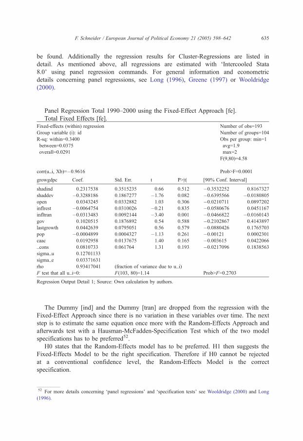
F. Schneider / European Journal of Political Economy 21 (2005) 598–642 635
be found. Additionally the regression results for Cluster-Regressions are listed in
detail. As mentioned above, all regressions are estimated with dIntercooled Stata
8.0T using panel regression commands. For general information and econometric
details concerning panel regressions, see Long (1996), Greene (1997) or Wooldridge
(2000).
Panel Regression Total 1990–2000 using the Fixed-Effect Approach [fe].
Total Fixed Effects [fe].
Fixed-effects (within) regression Number of obs=193Group variable (i): id Number of groups=104
R-sq: within=0.3400 Obs per group: min=1
between=0.0375 avg=1.9
overall=0.0291 max=2
F(9,80)=4.58
corr(u_i, Xb)=�0.9616 ProbNF=0.0001
growgdpc Coef. Std. Err. t PN|t| [90% Conf. Interval]
shadind 0.2317538 0.3515235 0.66 0.512 �0.3532252 0.8167327
shaddev �0.3288186 0.1867277 �1.76 0.082 �0.6395566 �0.0180805
open 0.0343245 0.0332882 1.03 0.306 �0.0210711 0.0897202
inflrest �0.0064754 0.0310026 �0.21 0.835 �0.0580676 0.0451167
infltran �0.0313483 0.0092144 �3.40 0.001 �0.0466822 �0.0160143
gov 0.1020515 0.1876892 0.54 0.588 �0.2102867 0.4143897
lastgrowth 0.0442639 0.0795051 0.56 0.579 �0.0880426 0.1765703
pop �0.0004899 0.0004327 �1.13 0.261 �0.00121 0.0002301
caac 0.0192958 0.0137675 1.40 0.165 �0.003615 0.0422066_cons 0.0810733 0.061764 1.31 0.193 �0.0217096 0.1838563
sigma_u 0.12701133
sigma_e 0.03371631
rho 0.93417041 (fraction of variance due to u_i)
F test that all u_i=0: F(103, 80)=1.14 ProbNF=0.2703
Regression Output Detail 1; Source: Own calculation by authors.
The Dummy [ind] and the Dummy [tran] are dropped from the regression with the
Fixed-Effect Approach since there is no variation in these variables over time. The next
step is to estimate the same equation once more with the Random-Effects Approach and
afterwards test with a Hausman-McFadden-Specification Test which of the two model
specifications has to be preferred52.
H0 states that the Random-Effects model has to be preferred. H1 then suggests the
Fixed-Effects Model to be the right specification. Therefore if H0 cannot be rejected
at a conventional confidence level, the Random-Effects Model is the correct
specification.
52 For more details concerning dpanel regressionsT and dspecification testsT see Wooldridge (2000) and Long
(1996).
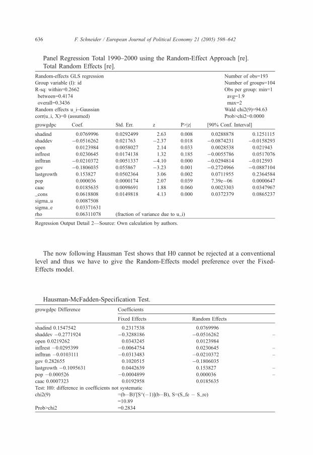
F. Schneider / European Journal of Political Economy 21 (2005) 598–642636
Panel Regression Total 1990–2000 using the Random-Effect Approach [re].
Total Random Effects [re].
Random-effects GLS regression Number of obs=193
Group variable (I): id Number of groups=104
R-sq: within=0.2662 Obs per group: min=1
between=0.4174 avg=1.9
overall=0.3436 max=2
Random effects u_i~Gaussian Wald chi2(9)=94.63
corr(u_i, X)=0 (assumed) ProbNchi2=0.0000
growgdpc Coef. Std. Err. z PN|z| [90% Conf. Interval]
shadind 0.0769996 0.0292499 2.63 0.008 0.0288878 0.1251115
shaddev �0.0516262 0.021763 �2.37 0.018 �0.0874231 �0.0158293
open 0.0123984 0.0058027 2.14 0.033 0.0028538 0.021943
inflrest 0.0230645 0.0174138 1.32 0.185 �0.0055786 0.0517076
infltran �0.0210372 0.0051337 �4.10 0.000 �0.0294814 �0.012593
gov �0.1806035 0.055867 �3.23 0.001 �0.2724966 �0.0887104
lastgrowth 0.153827 0.0502364 3.06 0.002 0.0711955 0.2364584
pop 0.000036 0.0000174 2.07 0.039 7.39e�06 0.0000647
caac 0.0185635 0.0098691 1.88 0.060 0.0023303 0.0347967_cons 0.0618808 0.0149818 4.13 0.000 0.0372379 0.0865237
sigma_u 0.0087508
sigma_e 0.03371631
rho 0.06311078 (fraction of variance due to u_i)
Regression Output Detail 2—Source: Own calculation by authors.
The now following Hausman Test shows that H0 cannot be rejected at a conventional
level and thus we have to give the Random-Effects model preference over the Fixed-
Effects model.
Hausman-McFadden-Specification Test.
growgdpc Difference Coefficients
Fixed Effects Random Effects
shadind 0.1547542 0.2317538 0.0769996
shaddev �0.2771924 �0.3288186 �0.0516262 –
open 0.0219262 0.0343245 0.0123984
inflrest �0.0295399 �0.0064754 0.0230645 –
infltran �0.0103111 �0.0313483 �0.0210372 –
gov 0.282655 0.1020515 �0.1806035
lastgrowth �0.1095631 0.0442639 0.153827 –
pop �0.000526 �0.0004899 0.000036 –
caac 0.0007323 0.0192958 0.0185635
Test: H0: difference in coefficients not systematic
chi2(9) =(b�B)V[S^(�1)](b�B), S=(S_fe � S_re)
=10.89
ProbNchi2 =0.2834
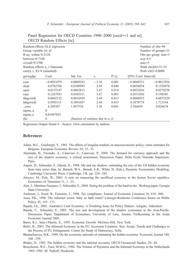
F. Schneider / European Journal of Political Economy 21 (2005) 598–642 637
Panel Regression for OECD Countries 1990–2000 [oecd==1 and re].
OECD Random Effects [re].
Random-effects GLS regression Number of obs=94
Group variable (i): id Number of groups=21
R-sq: within=0.2128 Obs per group: min=3
between=0.7168 avg=4.5
overall=0.3700 max=5
Random effects u_i~Gaussian Wald chi2(6)=51.10
corr(u_i, X)=0 (assumed) ProbNchi2=0.0000
growgdpc Coef. Std. Err. z PN|z| [95% Conf. Interval]
year �0.0031079 0.0009262 �3.36 0.001 �0.0049231 �0.0012926
shad 0.0782766 0.0380983 2.05 0.040 0.0036054 0.1529478
open 0.0155147 0.0062813 2.47 0.014 0.0032036 0.0278258
caac 0.1267053 0.0365311 3.47 0.001 0.0551056 0.198305
fdigrowth 0.0042132 0.0016938 2.49 0.013 0.0008935 0.0075329
labgrowth 0.9505111 0.3891057 2.44 0.015 0.1878778 1.713144_cons 6.205567 1.847538 3.36 0.001 2.584459 9.826674
sigma_u 0
sigma_e 0.01887023
rho 0 (fraction of variance due to u_i)
Regression Output Detail 6—Source: Own calculation by authors.
References
Adam, M.C., Ginsburgh, V., 1985. The effects of irregular markets on macroeconomic policy: some estimates for
Belgium. European Economic Review 29, 15–33.
Ahumada, H., Facundo, A., Canavese A., Canavese, P., 2004. The demand for currency approach and the
size of the shadow economy: a critical assessment. Discussion Paper, Delta Ecole Normale Superieure,
Paris.
Aigner, D., Schneider, F., Ghosh, D., 1988. Me and my shadow: estimating the size of the US hidden economy
from time series data. In: Barnett, W.A., Berndt, E.R., White, H. (Eds.), Dynamic Econometric Modeling.
Cambridge University Press, Cambridge, UK, pp. 224–243.
Alexeev, M., Pyle, W., 2003. A note on measuring the unofficial economy in the former Soviet republics.
Economics of Transition 11, 1–23.
Alm, J., Martinez-Vazquez, J., Schneider, F., 2004. Sizing the problem of the hard-to-tax. Working paper, Georgia
State University.
Andreoni, J., Erard, B., Feinstein, J., 1998. Tax compliance. Journal of Economic Literature 36, 818–860.
Asea, P.K., 1996. The informal sector: baby or bath water? Carnegie-Rochester Conference Series on Public
Policy 45, 163–171.
Bajada, Ch., 2002. Australia’s Cash Economy: A Troubling Issue for Policy Makers. Ashgate, Aldershort.
Bajada, C., Schneider, F., 2003. The size and development of the shadow economies in the Asia-Pacific.
Discussion Paper, Department of Economics, University of Linz, Austria. Forthcoming in the Asian
Economic Journal 2005.
Barro, R.J., Sala-i-Martin, X., 1995. Economic Growth. McGraw-Hill, New York.
Belev, B., 2003. The Informal Economy in the EU Accession Countries: Size, Scope, Trends and Challenges to
the Process of EU Enlargement. Center for Study of Democracy, Sofia.
Bhattacharyya, D.K., 1999. On the economic rationale of estimating the hidden economy. Economic Journal 109,
348–359.
Blades, D., 1982. The hidden economy and the national accounts. OECD Occasional Studies, 28–44.
Boeschoten, W.C., Fase, M.M.G., 1984. The Volume of Payments and the Informal Economy in the Netherlands
1965–1982. M. Nijhoff, Dordrecht.
F. Schneider / European Journal of Political Economy 21 (2005) 598–642638
Brehm, J.W., 1966. A Theory of Psychological Reactance. Academic Press, New York.
Brehm, J.W., 1972. Responses to Loss of Freedom: A Theory of Psychological Reactance. General Learning
Press, Morristown.
Breton, T.R., 2001. Missing data and omitted variables: continuing the search for a complete Solow growth
model. Working paper, George Mason University, Fairfax, Virginia.
Cagan, P., 1958. The demand for currency relative to the total money supply. Journal of Political Economy 66,
302–328.
Chatterjee, S., Chaudhury K., Schneider, F., 2003. The size and development of the Indian shadow economy and
a comparison with other 18 Asian countries: an empirical investigation. Discussion Paper, Department of
Economics, University of Linz, Austria.
Clotefelter, C.T., 1983. Tax evasion and tax rates: an analysis of individual returns. Review of Economic Statistics
65, 363–373.
Contini, B., 1981. Labor market segmentation and the development of the parallel economy: the Italian
experience. Oxford Economic Papers 33, 401–412.
Dallago, B., 1990. The Irregular Economy: The bUnderground EconomyQ and the bBlack Labour MarketQ.Dartmouth Publishing, UK.
Del’Anno, R., 2003. Estimating the shadow economy in Italy: a structural equation approach. Discussion Paper,
Department of Economics and Statistics, University of Salerno.
Del’Anno, R., Schneider, F., 2004. The shadow economy of Italy and other OECD countries: what do we know?
University of Linz. Department of Economics Discussion Paper.
Del Boca, D., 1981. Parallel economy and allocation of time. Micros (Quarterly Journal of Microeconomics) 4,
13–18.
Del Boca, D., Forte, F., 1982. Recent empirical surveys and theoretical interpretations of the parallel economy in
Italy. In: Tanzi, V. (Ed.), The Underground Economy in the United States and Abroad. Lexington Books,
Lexington, MA, pp. 160–178.
Feige, E.L., 1986. A re-examination of the bunderground economyQ in the United States. IMF Staff Papers 33,
768–781.
Feige, E.L. (Ed.), The Underground Economies: Tax Evasion and Information Distortion. Cambridge University
Press, Cambridge, UK.
Feige, E.L., 1994. The underground economy and the currency enigma. Supplement to Public Finance/Finances
Publiques 49, 119–136.
Feige, E.L., 1996. Overseas holdings of U.S. currency and the underground economy. In: Pozo, S. (Ed.),
Exploring the Underground Economy. W.E. Upjohn Institute for Employment Research, Kalamazoo, MI,
pp. 5–62.
Fleming, M.H., Roman, J., Farrel, G., 2000. The shadow economy. Journal of International Affairs 53, 64–89.
Franz, A., 1983. Wie grog ist die bschwarzeQ Wirtschaft? Mitteilungsblatt der Osterreichische Statistische
Gesellschaft 49, 1–6.
Frey, B.S., Pommerehne, W.W., 1984. The hidden economy: state and prospect for measurement. Review of
Income and Wealth 30, 1–23.
Frey, B.S., Weck, H., 1983a. Bureaucracy and the shadow economy: a macro-approach. In: Hanusch, H. (Ed.),
Anatomy of Government Deficiencies. Springer, Berlin, pp. 89–109.
Frey, B.S., Weck, H., 1983b. Estimating the shadow economy: a dnaiveT approach. Oxford Economic Papers 35,
23–44.
Frey, B.S., Weck-Hannemann, H., 1984. The hidden economy as an bunobservedQ variable. European Economic
Review 26, 33–53.
Frey, B.S., Weck, H., Pommerehne, W.W., 1982. Has the shadow economy grown in Germany? An exploratory
study. Weltwirtschaftliches Archiv 118, 499–524.
Friedman, E., Johnson, S., Kaufmann, D., Zoido-Labton, P., 2000. Dodging the grabbing hand: the determinants
of unofficial activity in 69 countries. Journal of Public Economics 76, 459–493.
Garcia, G., 1978. The currency ratio and the subterranean economy. Financial Analysts Journal 69, 64–66.
Gerxhani, K., 2003. The informal sector in developed and less-developed countries: a literature survey. Public
Choice 114, 295–318.
F. Schneider / European Journal of Political Economy 21 (2005) 598–642 639
Giles, D.E.A., 1997a. Causality between the measured and underground economies in New Zealand. Applied
Economics Letters 4, 63–67.
Giles, D.E.A., 1997b. Testing the asymmetry in the measured and underground business cycles in New Zealand.
Economic Record 71, 225–232.
Giles, D.E.A., 1999a. Measuring the hidden economy: implications for econometric modeling. Economic Journal
109, 370–380.
Giles, D.E.A., 1999b. Modeling the hidden economy in the tax-gap in New Zealand. Empirical Economics 24,
621–640.
Giles, D.E.A., 1999c. The rise and fall of the New Zealand underground economy: are the reasons symmetric?
Applied Economics Letters 6, 185–189.
Giles, D.E.A., Tedds, L.M., 2002. Taxes and the Canadian underground economy. Canadian Tax Paper, vol. 106.
Canadian Tax Foundation, Toronto.
Giles, D.E.A., Tedds, L.M., Gugsa, W., 2002. The Canadian underground and measured economies. Applied
Economics 34, 2347–2352.
Greene, W.H., 1997. Econometric Analysis. Prentice Hall International, London.
Gutmann, P.M., 1977. The subterranean economy. Financial Analysts Journal 34 (1), 24–27.
Helberger, C., Knepel, H., 1988. How big is the shadow economy? A re-analysis of the unob-
served-variable approach of B.S. Frey and H. Weck-Hannemann. European Economic Journal 32,
965–976.
Hill, R., Kabir, M., 1996. Tax rates, the tax mix, and the growth of the underground economy in Canada: what can
we infer? Canadian Tax Journal/Revue Fiscale Canadienne 44, 1552–1583.
Houston, J.F., 1987. Estimating the size and the implication of the underground economy. Working Paper 87-9,
Federal Reserve Bank, Philadelphia, USA.
IRS, 1979. Estimates of Income Unreported on Individual Tax Reform. Internal Revenue Service, U.S.
Department of the Treasury, Washington, DC.
IRS, 1983. Income Tax Compliance Research: Estimates for 1973–81. Internal Revenue Service, U.S.
Department of the Treasury, Washington, DC.
Isachsen, A.J., Strom, S., 1985. The size and growth of the hidden economy in Norway. Review of Income and
Wealth 31, 21–38.
Isachsen, A.J., Klovland, J., Strom, S., 1982. The hidden economy in Norway. In: Tanzi, V. (Ed.), The
Underground Economy in the United States and Abroad. DC Heath, Lexington Books, Lexington, MA,
pp. 209–231.
Johnson, S., Kaufmann, D., Shleifer, A., 1997. The Unofficial Economy in Transition. Brookings Papers on
Economic Activity. Brookings Institute, Washington, DC.
Johnson, S., Kaufmann, D., Zoido-Lobaton, P., 1998a. Regulatory discretion and the unofficial economy. The
American Economic Review 88, 387–392.
Johnson, S., Kaufmann, D., Zoido-Lobaton, P., 1998b. Corruption, public finances and the unofficial economy.
Discussion paper, The World Bank, Washington, DC.
Karmann, A., 1986. Monet7re Ans7tze zur Erfassung der Schattenwirtschaft: Ein Vergleich verschiedener
Messans7tze. Kredit und Kapitel 19, 233–247.
Karmann, A., 1990. Schattenwirtschaft und ihre Ursachen: Eine empirische Analyse zur Schwarzwirtschaft und
Selbstversorgung in der Bundesrepublik Deutschland. Zeitschrift fqr Wirtschafts- und Sozialwissenschaften
(ZWS) 110, 185–206.
Kaufmann, D., Kaliberda, A., 1996. Integrating the unofficial economy into the dynamics of post socialist
economies: a framework of analyses and evidence. In: Kaminski, B. (Ed.), Economic Transition in Russia and
the New States of Eurasia. M.E. Sharpe, London, pp. 81–120.
Kirchg7ssner, G., 1983. Size and development of the West German shadow economy, 1955–1980. Zeitschrift fqrdie Gesamte Staatswissenschaft 139, 197–214.
Kirchg7ssner, G., 1984. Verfahren zur Erfassung des in der Schattenwirtschaft erarbeiteten Sozialprodukts.
Allgemeines Statistisches Archiv 68, 378–405.
Kirchler, E., Maciejovsky, B., Schneider, F., 2002. Everyday representations of tax avoidance, tax evasion and tax
flight: do legal differences matter? Economic Psychology 8, 1–19.
F. Schneider / European Journal of Political Economy 21 (2005) 598–642640
Klovland, J., 1984. Tax evasion and the demand for currency in Norway and Sweden: is there a hidden
relationship? Scandinavian Journal of Economics 86, 423–439.
Lacko, M., 1996. Hidden economy in East-European countries in international comparison. Working paper,
International Institute for Applied Systems Analysis (IIASA), Laxenburg.
Lacko, M., 1998. The hidden economies of Visegrad countries in international comparison: a household
electricity approach. In: Halpern, L., Wyplosz, C. (Eds.), Hungary: Towards a Market Economy. Cambridge
University Press, Cambridge, UK, pp. 128–152.
Lacko, M., 1999. Hidden economy – an unknown quantitiy? Comparative analyses of hidden economies in
transition countries in 1989–95. Working paper 9905, Department of Economics, University of Linz, Austria.
Lacko, M., 2000. Hidden economy—an unknown quantity?: comparative analysis of hidden economics in
Transition countries 1989–95. Economics of Transition 8, 117–149.
Langfeldt, E., 1984. The unobserved economy in the Federal Republic of Germany. In: Feige, E.L. (Ed.), The
Unobserved Economy. Cambridge University Press, Cambridge, UK, pp. 236–260.
Lippert, O., Walker, M., 1997 (Eds.), The Underground Economy: Global Evidences of its Size and Impact. The
Frazer Institute, Vancouver, BC.
Lizzeri, C., 1979. Mezzogiorno in Controluce. Enel, Naples.
Loayza, N.V., 1996. The economics of the informal sector: a simple model and some empirical evidence from
Latin America. Carnegie-Rochester Conference Series on Public Policy 45, 129–162.
Long, S.J., 1996. Regression Models for Categorical and Limited Dependent Variables. Sage Publications,
London.
MacAfee, K., 1980. A glimpse of the hidden economy in the national accounts. Economic Trends 136, 81–87.
Mauleon, I., 1998. Quantitative estimation of the Spanish underground economy. Discussion paper, Department
of Economics and History, University of Salamanka.
Mogensen, G.V., Kvist, H.K., Kfrmendi, E., Pedersen, S., 1995. The Shadow Economy in Denmark 1994:
Measurement and Results. Study no. 3. The Rockwool Foundation Research Unit, Copenhagen.
Morris, B., 1993. Editorial statement. International Economic Insides, vol. IV. International Statistical Yearbook,
Budapest.
Mummert, A., Schneider, F., 2001. The German shadow economy: parted in a united Germany? Finanzarchiv 58,
260–285.
Neck, R., Hofreither, M., Schneider, F., 1989. The consequences of progressive income taxation for the shadow
economy: some theoretical considerations. In: Boes, D., Felderer, B. (Eds.), The Political Economy of
Progressive Taxation. Springer, Heidelberg, pp. 149–176.
O’Higgins, M., 1989. Assessing the underground economy in the United Kingdom. In: Feige, E.L. (Ed.), The
Underground Economies: Tax Evasion and Information Distortion. Cambridge University Press, Cambridge,
UK, pp. 175–195.
O’Neill, D.M., 1983. Growth of the underground economy 1950–81: some evidence from the current population
survey. Study for the Joint Economic Committee. U.S. Congress Joint Committee Print, U.S. Gov. Printing
Office, Washington, DC, pp. 98–122.
Park, T., 1979. Reconciliation Between Personal Income and Taxable Income. Bureau of Economic Analysis,
Washington, DC, pp. 1947–1977.
Pedersen, S., 2003. The Shadow Economy in Germany, Great Britain and Scandinavia: A Measurement Based on
Questionnaire Service. Study No. 10. The Rockwool Foundation Research Unit, Copenhagen.
Pelzmann, L., 1988. Wirtschaftspsychologie. Arbeitslosenforschung, Schattenwirtschaft, Steuerpsychologie.
Springer, Vienna.
Petersen, H.-G., 1982. Size of the public sector, economic growth and the informal economy: development trends
in the Federal Republic of Germany. Review of Income and Wealth 28, 191–215.
Pissarides, C., Weber, G., 1988. An expenditure–based estimate of Britain’s black economy. CLE Working Papers
104 (London). 40 pp.
Pommerehne, W.W., Schneider, F., 1985. The decline of productivity growth and the rise of the shadow economy
in the U.S., Working Paper 85-9, University of Aarhus.
Portes, A., 1996. The informal economy. In: Pozo, S. (Ed.), Exploring the Underground Economy. W.E. Upjohn
Institute for Employment Research, Kalamazoo, pp. 147–165.
F. Schneider / European Journal of Political Economy 21 (2005) 598–642 641
Pozo, S., 1996 (Ed.), Exploring the Underground Economy: Studies of Illegal and Unreported Activity. W.E.
Upjohn, Institute for Employment Research, Michigan.
Quirk, P.J., 1996. Macroeconomic implications of money laundering. IMF working paper WP/96/66,
International Monetary Fund, Washington, DC.
Rogoff, K., 1998. Blessing or curse? Foreign and underground demand for euro notes. Economic Policy: The
European Forum 26, 261–304.
Schneider, F., 1986. Estimating the size of the Danish shadow economy using the currency demand approach: an
attempt. The Scandinavian Journal of Economics 88, 643–668.
Schneider, F., 1994a. Measuring the size and development of the shadow economy: can the causes be found and
the obstacles be overcome? In: Brandstaetter, H., Gqth, W. (Eds.), Essays on Economic Psychology. Springer,
Berlin, pp. 193–212.
Schneider, F., 1994b. Can the shadow economy be reduced through major tax reforms? An empirical
investigation for Austria. Supplement to Public Finance/Finances Publiques 49, 137–152.
Schneider, F., 1997. The shadow economies of Western Europe. Journal of the Institute of Economic Affairs 17,
42–48.
Schneider, F., 1998a. Further empirical results of the size of the shadow economy of 17 OECD-countries over
time. Paper Presented at the 54th Congress of the IIPF Cordova, Argentina, and Discussion Paper, Department
of Economics, University of Linz, Linz, Austria.
Schneider, F., 1998b. Stellt das Anwachsen der Schwarzarbeit eine wirtschaftspolitische Herausforderung dar?
Einige Gedanken aus volkswirtschaftlicher Sicht. Mitteilungen des Instituts fqr Angewandte Wirtschaftsfor-
schung (IAW) I/98, 4–13. (Linz).
Schneider, F., 2000. The increase of the size of the shadow economy of 18 OECD-Countries: some preliminary
explanations. Paper presented at the Annual Public Choice Meeting, Charleston, SC.
Schneider, F., 2003. The shadow economy. In: Rowley, C.K., Schneider, F. (Eds.), Encyclopedia of Public
Choice. Kluwer Academic Publishers, Dordrecht.
Schneider, F., Enste, D., 2000. Shadow economies: size, causes, and consequences. Journal of Economic
Literature 38, 77–114.
Schneider, F., Enste, D., 2002. The Shadow Economy: Theoretical Approaches, Empirical Studies, and Political
Implications. Cambridge University Press, Cambridge UK.
Schneider, F., Hofreither, M.F., Neck, R., 1989. The consequences of a changing shadow economy for the official
economy: some empirical results for Austria. In: Boes, D., Felderer, B. (Eds.), The Political Economy of
Progressive Taxation. Springer, Heidelberg, pp. 181–211.
Simon, C.B., Witte, A.G., 1982. Beating the System: The Underground Economy. Urban House, Boston, MA.
Smith, J.D., 1985. Market motives in the informal economy. In: Gaertner, W., Wenig, A. (Eds.), The Economics
of the Shadow Economy. Springer, Heidelberg, pp. 161–177.
Smith, P., 1994. Assessing the size of the underground economy: the Canadian statistical perspectives. Canadian
Economic Observer 11, 16–33.
Spiro, P.S., 1993. Evidence of a post-GST increase in the underground economy. Canadian Tax Journal/Revue
Fiscale Canadienne 41, 247–258.
Tanzi, V., 1980. The underground economy in the United States: estimates and implications. Banca Nazionale del
Lavoro 135, 427–453.
Tanzi, V. (Ed.), 1982. The Underground Economy in the United States and Abroad. Lexington Books, Lexington,
MA.
Tanzi, V., 1982. A second (and more skeptical) look at the underground economy in the United States. In:
Tanzi, V. (Ed.), The Underground Economy in the United States and Abroad. Lexington Books, Lexington,
MA, pp. 38–56.
Tanzi, V., 1983. The underground economy in the United States: annual estimates, 1930–1980. IMF Staff Papers
30, 283–305.
Tanzi, V., 1986. The underground economy in the United States: reply to comments by Feige, Thomas, and
Zilberfarb. IMF Staff Papers 33, 799–811.
Tanzi, V., 1999. Uses and abuses of estimates of the underground economy. Economic Journal 109, 338–340.
Thomas, J.J., 1986. The underground economy in the United States: comment on Tanzi. IMF Staff Papers 33,
782–789.
F. Schneider / European Journal of Political Economy 21 (2005) 598–642642
Thomas, J.J., 1992. Informal Economic Activity, LSE Handbooks in Economics. Harvester Wheatsheaf,
London.
Thomas, J.J., 1999. Quantifying the black economy: dmeasurement without theoryT yet again? Economic Journal
109, 381–389.
Weck, H., 1983. Schattenwirtschaft: Eine Mfglichkeit zur Einschr7nkung der fffentlichen Verwaltung? Eine
fkonomische Analyze, Bern-Frankfurt.
Williams, C.C., Windebank, J., 1995. Black market work in the European Community: peripheral work for
peripheral localities? International Journal of Urban and Regional Research 19, 23–39.
Witte, A.D., 1987. The nature and extend of unreported activity: a survey concentrating on a recent US research.
In: Alessandrini, S., Dallago, B. (Eds.), The Unofficial Economy: Consequences and Perspectives in Different
Economic Systems. Gower, Aldershot.
Wooldridge, J.M., 2000. Introductory Econometrics. South Western College Publishing, USA.
Zilberfarb, B.-Z., 1986. Estimates of the underground economy in the United States, 1930–80. IMF Staff Papers
33, 790–798.