H:\eggrafa\personal\CV_tsili\CVtheo_en_03_web\compnets_public\serica_w_web.doc 1

SERICA_ω. An extension of the SERICA algorithm

G. I. Mousadis1, T. A. Tsiligirides1 and M. P. Bekakos2

1 Informatics Laboratory, General Sciences Department, Agricultural University of Athens, Athens 11855, Greece,

2 Laboratory of Digital Systems, Department of Electrical and Computer Engineering, School of Engineering, Democritus University of Thrace, Xanthi 67100, Greece,

Abstract This work presents an extension of a recently developed scheme, namely the Simple Explicit Rate Identification with Congestion Avoidance (SERICA) algorithm, which regulates the ABR traffic flow in an ATM network. Like SERICA, the new scheme, which is called SERICA_ω, takes into account the load and the queue length per VC, calculates the first approximation of the ER field of the BRM cell, and then it informs the switch accordingly. Because of the low buffer availability, the network administrator may not be able to initialize a new session. The solution of the above problem is given by means of deriving a new control function family for the SERICA_ω algorithm. This function has the property to decrease the average available queue length of the switch at about O(q1/ω), where q is the average queue length of the SERICA_1, i.e., the basic SERICA. The above model is calibrated to use different values of ω, in order to provide a guaranteed ABR service with short buffer availability (or, a limited queue length). Keywords - SERICA_ω algorithm, SERICA algorithm, ERICA algorithm, TCP over ATM, extended ABR, ABR, Differentiated Services.

1. INTRODUCTION As it is well known, Transmission Control Protocol (TCP), together with User Datagram Protocol (UDP), carries a significant amount of today’s Internet traffic. It serves applications like www (HTTP), file transfer (FTP), E-mail (SMTP), remote access (Telnet), etc., as a means of reliable transport. TCP implements the additive increase multiplicative decrease scheme to achieve a fair division of available bandwidth in a network amongst competing sources. It is a window-based method in which, at any time, window size number of data packets are allowed in the network. This window size is additively increased roughly every Fixed Round Trip Time (FRTT) until congestion is detected. Then, a multiplicatively decreased mechanism is applied. In the current implementations of TCP the detection of congestion is detected implicitly, namely, by the

H:\eggrafa\personal\CV_tsili\CVtheo_en_03_web\compnets_public\serica_w_web.doc 2

loss of packets. The diverse and changing nature of service requirements among the emerging Internet applications, desires a network architecture that is both flexible and able to distinguish their needs. A successful deployment of such architecture is offered by the so-called Differentiated Services (Diff Serv), which necessitates simple mechanisms inside the network. For example, a basic characteristic of Diff Serv architecture is the use of the same flow control algorithm in order to serve the different Type of Services (ToS), namely the Internet based applications, which have been classified according to their traffic description (see also Fujitsu, 2000). The Diff Serv architecture is based on a detailed contract between the Network Service Provider (NSP) and a user, which offers access on call. Thus, a connection is accepted or dropped by the NSP depending on the network resource availability. When accepted the requested QoS of the corresponding ToS of the application will be provided and the NSP will serve the user properly using the traffic descriptor set of parameters already negotiated in their contract. The above interface operates either with the TCP, or with the UDP. However, our focus is on the TCP since it is a connection-oriented protocol using a feedback window adjusted mechanism in a client-server loop.

From the above it appears that an interesting problem is to support integrated Internet applications, which are based on Diff Serv architecture, over the ABR traffic. Note that in an ATM network only the ABR service is able to guarantee an adjusted to the feedback, end-to-end, flow control traffic. For this reason the ABR service is best suited to support the TCP environment. According to the ATM FORUM (1996) (ATM FORUM Traffic Management Spec. Version 4.0), an ABR connection presumes a traffic contract supporting a MCR (Minimum Cell Rate), a PCR (Peak Cell Rate) and data transfer conforming with a CDVT (Cell Delay Variation Tolerance). In order to serve all kind of traffic, ATM has to guarantee that the maximum Cell Transfer Delay (maxCTD) and the deterministic part of the traffic flow, namely the Sustainable Cell Rate (SCR) are taking some predefined values. This last property gives rise to support the Diff Serv architecture through the extended ABR service and the corresponding traffic descriptor set of parameters (Mousadis (2001) and Mousadis & Tsiligirides (2002)). In particular, the unpredictable ABR traffic requires a suitable flow control mechanism to automatically adjust the source emission rate according to the service rate fluctuations of the switches. This traffic is desirable to be served from a globally stable feedback mechanism, in order to operate safely with almost 100% utilization. However, to prevent buffer overflow, this mechanism should use a target threshold of the queuing delay (T0). Thus, in a steady state, i.e., when the Allowed Cell Rate (ACR) of the switch remains constant for more than one time interval, the target queuing delay, which depends on the current ACR, may determine a stable operational point (ACR, qst) of the corresponding target queue length (qst).

To serve the ABR traffic, the ATM Forum proposed the Explicit Rate (ER) based switch schemes, which are based on the leaky bucket model and offered as an alternative of a window based or a credit based schemes. The ER based closed-loop approach uses feedback acknowledgements via the Resource Management (RM) cells in both directions: in the Forward (from the source to the destination – FRM cells) and in the Backward (from the destination back to the source – BRM cells). To avoid congestion, a hop-by-hop strategy that uses the Virtual Source / Virtual Destination (VS/VD) property

3

in a tandem configuration may be adopted. The RM cells are used to control the VS emission rate, according to the VD requests. In particular, through the ER Field (ERF) of the BRM cells, the VD acknowledges the desirable source emission rate of the next time instant, namely the Worst Case Traffic (WCT) scenario, in which MACR(tn+1) = ERF(tn); tn = τ n, n = 0, 1, 2, ... .

The ER-based switch algorithms are divided into two major classes. The first class includes the Proportional Control type algorithms, which are locally unstable, whereas the second class includes the Congestion Avoidance algorithms (ERICA and ERICA+), which are globally stable. In particular, these last type of algorithms: achieve stability by using some artificial parameters optimized by simulation, ensure a target utilization with a predetermined bandwidth level (Kalyanaraman et

al. (2001)), provide max-min fairness with MCR criterion. However, according to the negotiated traffic descriptor, these algorithms do not guarantee for a specific SCR, i.e., they cannot support the extended ABR service.

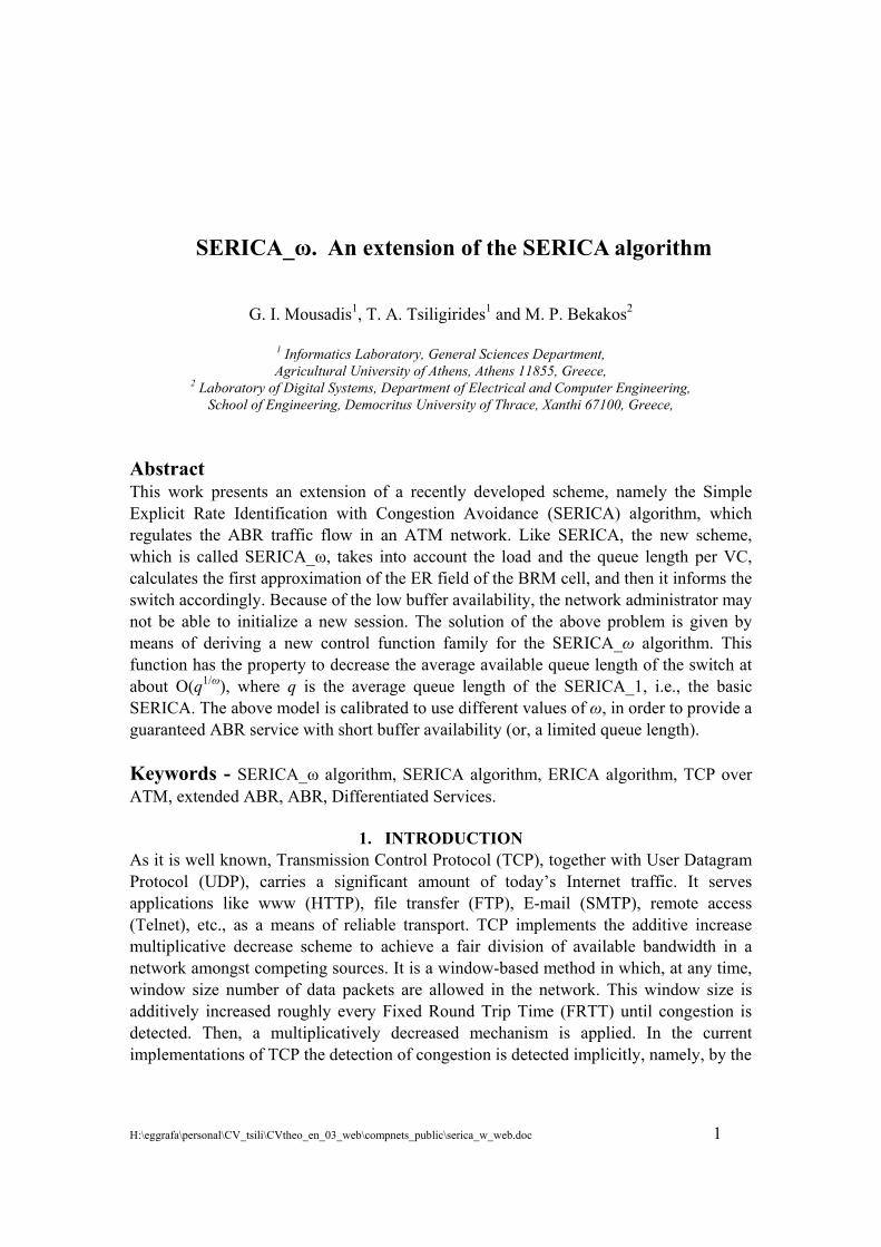
ERICA type algorithms have been developed into the context of a Continuous State Leaky-Bucket, which has been proposed by the ATM Forum as a reference algorithm, with aim to determine some useful parameters at a connection set-up (Figure 1a). The algorithmic scheme has a close relationship with the single server queue model with deterministic service time (Mignault et al., (1996) ; Mousadis et al. (1996)). An equivalent problem is how to avoid overflow when a fluid tank is refilled (Figure 1b). The floater control valve regulates the input rate in accordance with the volume of the fluid stored into the tank and the input – output fluid flows of the tank. Assuming that the ERF of the BRM cell presents the Worst Case of Traffic (WCT) input rate and that the ACR is the output rate of the fluid tank (or the ACR(tn) of the switch at the current time instant tn = nτ, n =0, 1, 2...), then a function f(q(tn)), which determines the input rate in accordance with the output rate and the fluid stored in the tank may be defined. Obviously, this function presents the up/down movement of the floater mechanical bar and is derived algorithmically in each time instant tn through the recursive equation: MACR(tn+1) = ERF(tn) = f(q(tn))·ACR(tn).

An interesting family of such queue control function has been introduced and

discussed by Kalyanaraman (1997). This function has the following form:

0

0 1

1 2

2

1, if 0

1, if ( )

1, if

, if

n

nn

n

n

q t q

q q t qf q t

q q t q

QDLF q q t

,

In the above, q0, q1 and q2, are the three different levels of the queue length whereas QDLF (Queuing Delay Limit Factor) is the lower bound of the function. Four such control functions, namely the step, the linear, the hyperbolic and the inverse hyperbolic have been tested so far. It has been showed that the inverse hyperbolic function is approximated through the use of two rectangular hyperbolic functions in which the target queue length is 1 and performs better than the other schemes. Note that the step scheme is the simplest to implement in hardware since it does not require actual calculation, the

4

linear scheme is implemented efficiently using shift operations for some of its parameters, whereas the hyperbolic scheme includes a division operation, which adds calculation complexity and needs much more execution time than the other schemes. However, a common disadvantage of all these functions is that they use arbitrary parameters, which need to be optimized by simulation. This is because of the ERICA and ERICA+ schemes are based on an approximation of the window of the source in a steady state condition. Following this, it is assumed that the window of the source depends only on the ACR of the source (i.e., it is independent of the queue length of the switches).

Figure 1: The block diagram of the source controller (a) (Leaky-Bucket problem) and its equivalent fluid tank overflow problem (b).

Into the above framework a recently developed algorithm (Mousadis & Tsiligirides (2002)) called Simple ERICA (SERICA) has shown an interesting superiority over the original ERICA and ERICA+ algorithms, in the following aspects: It obtains analytically a stable equilibrium point, using O(1) calculations. It adjusts the optimized parameters in each time slot according with the availability

of the network resources. It guarantees a specific SCR, when a queue length of O(PCR) is allocated to the VC. It uses more than one BRM cells in order to manage in a better way the VS emission

rate by taking into account the latest arrived information about a persistent congestion.

The contribution of this work is to extend the SERICA algorithm, in order to

minimize further the queuing delay, namely, by giving the possibility to initialize a new session when a queue length less than O(PCR) is allocated in the VC. The extended algorithm, called SERICA_ω, is based on both the model set-up and the rate control model of the ER scheme (Mousadis & Tsiligirides (2002)). Note that in order to increase the network operability a new parameter ω is introduced. This parameter is determined during the call set-up by the network administrator in order to reduce the average queue length of the switch at about O(PCR1/ω) in a steady-state. As it appears, the results are comparable with those obtained from the SERICA and ERICA algorithms, in the sense that in a steady-state the throughput of the new algorithm achieves nearly 100% of the available bandwidth, whereas in the non-steady state it does not drop from 79%.

Maximum inputsource capability

Feedback informationMaximum output source capability.Parameters monitored on the server(input, output, buffer occupancy etc).

Controller of the sourceAllowed output

source capability

(a)

out

in Volume of the fluid into the tank (b)

5

The organization of this paper is as follows. Section 2 presents a review of the

SERICA algorithm, Section 3 provides the model, the numerical and the stability analysis of the proposed SERICA_ω algorithm, whereas Section 4 shows some interesting simulation results. Finally, the conclusions are presented in Section 5.

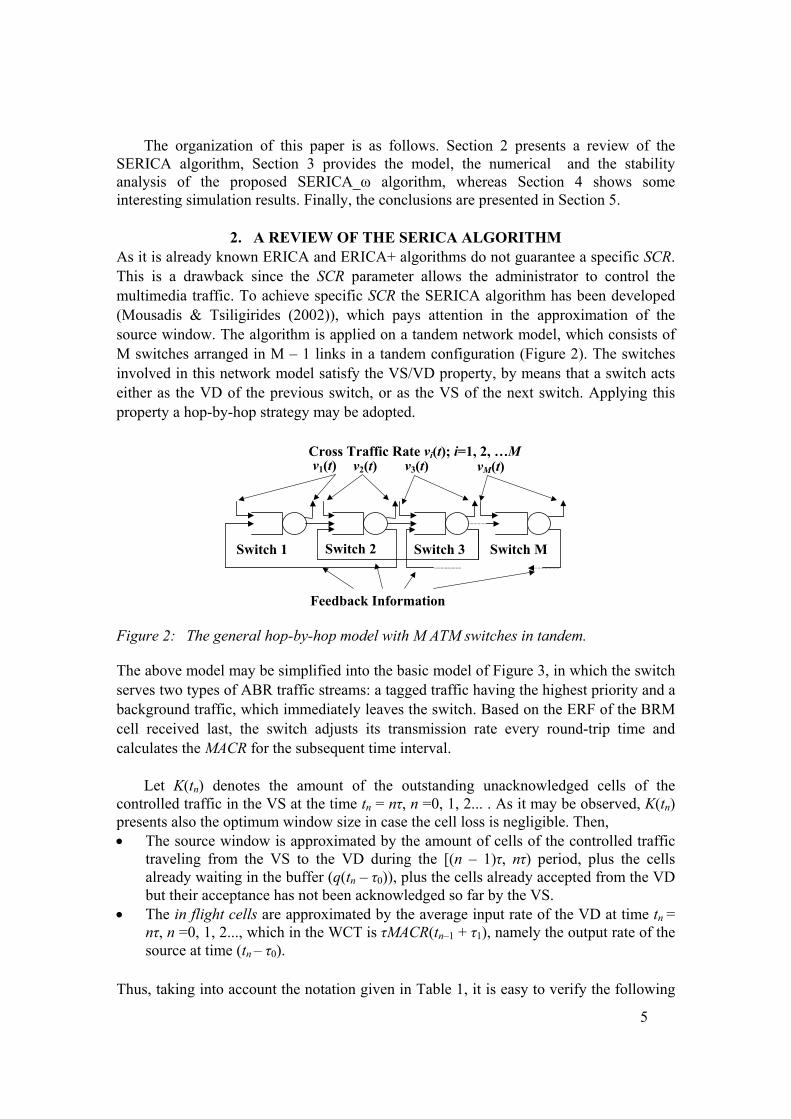
2. A REVIEW OF THE SERICA ALGORITHM As it is already known ERICA and ERICA+ algorithms do not guarantee a specific SCR. This is a drawback since the SCR parameter allows the administrator to control the multimedia traffic. To achieve specific SCR the SERICA algorithm has been developed (Mousadis & Tsiligirides (2002)), which pays attention in the approximation of the source window. The algorithm is applied on a tandem network model, which consists of M switches arranged in M – 1 links in a tandem configuration (Figure 2). The switches involved in this network model satisfy the VS/VD property, by means that a switch acts either as the VD of the previous switch, or as the VS of the next switch. Applying this property a hop-by-hop strategy may be adopted.

Switch 1

Feedback Information

Cross Traffic Rate νi(t); i=1, 2, …M ν1(t) ν2(t) ν3(t) νM(t)

Switch 2 Switch 3 Switch M

Figure 2: The general hop-by-hop model with M ATM switches in tandem.

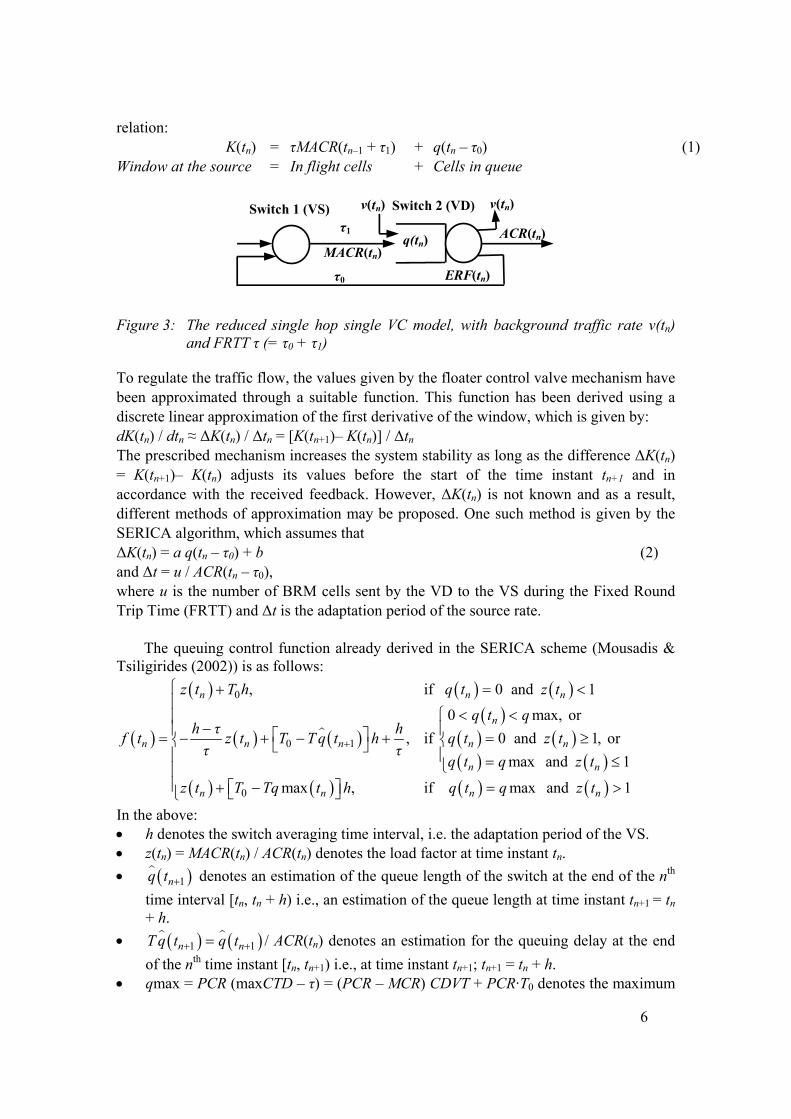
The above model may be simplified into the basic model of Figure 3, in which the switch serves two types of ABR traffic streams: a tagged traffic having the highest priority and a background traffic, which immediately leaves the switch. Based on the ERF of the BRM cell received last, the switch adjusts its transmission rate every round-trip time and calculates the MACR for the subsequent time interval.

Let K(tn) denotes the amount of the outstanding unacknowledged cells of the controlled traffic in the VS at the time tn = nτ, n =0, 1, 2... . As it may be observed, K(tn) presents also the optimum window size in case the cell loss is negligible. Then, The source window is approximated by the amount of cells of the controlled traffic

traveling from the VS to the VD during the [(n – 1)τ, nτ) period, plus the cells already waiting in the buffer (q(tn – τ0)), plus the cells already accepted from the VD but their acceptance has not been acknowledged so far by the VS.

The in flight cells are approximated by the average input rate of the VD at time tn = nτ, n =0, 1, 2..., which in the WCT is τMACR(tn–1 + τ1), namely the output rate of the source at time (tn – τ0).

Thus, taking into account the notation given in Table 1, it is easy to verify the following

6

relation: K(tn) = τMACR(tn–1 + τ1) + q(tn – τ0) (1)

Window at the source = In flight cells + Cells in queue

Switch 1 (VS) Switch 2 (VD)

τ1

τ0

ν(tn) ν(tn)

MACR(tn)ACR(tn)q(tn)

ERF(tn)

Figure 3: The reduced single hop single VC model, with background traffic rate ν(tn)

and FRTT τ (= τ0 + τ1)

To regulate the traffic flow, the values given by the floater control valve mechanism have been approximated through a suitable function. This function has been derived using a discrete linear approximation of the first derivative of the window, which is given by: dK(tn) / dtn ≈ ΔK(tn) / Δtn = [K(tn+1)– K(tn)] / Δtn The prescribed mechanism increases the system stability as long as the difference ΔK(tn) = K(tn+1)– K(tn) adjusts its values before the start of the time instant tn+1 and in accordance with the received feedback. However, ΔK(tn) is not known and as a result, different methods of approximation may be proposed. One such method is given by the SERICA algorithm, which assumes that ΔK(tn) = a q(tn – τ0) + b (2) and Δt = u / ACR(tn – τ0), where u is the number of BRM cells sent by the VD to the VS during the Fixed Round Trip Time (FRTT) and Δt is the adaptation period of the source rate.

The queuing control function already derived in the SERICA scheme (Mousadis & Tsiligirides (2002)) is as follows:

0

0 1

0

, if 0 and 1

0 max, or

, if 0 and 1, or

max and 1

max , if max and 1

n n n

n

n n n n n

n n

n n n n

z t T h q t z t

q t qh τ h

f t z t T T q t h q t z tτ τ

q t q z t

z t T Tq t h q t q z t

In the above: h denotes the switch averaging time interval, i.e. the adaptation period of the VS. z(tn) = MACR(tn) / ACR(tn) denotes the load factor at time instant tn.

1nq t denotes an estimation of the queue length of the switch at the end of the nth

time interval [tn, tn + h) i.e., an estimation of the queue length at time instant tn+1 = tn + h.

1 1n nT q t q t / ACR(tn) denotes an estimation for the queuing delay at the end

of the nth time instant [tn, tn+1) i.e., at time instant tn+1; tn+1 = tn + h. qmax = PCR (maxCTD – τ) = (PCR – MCR) CDVT + PCR·T0 denotes the maximum

7

threshold of the queue length of the switch.

8

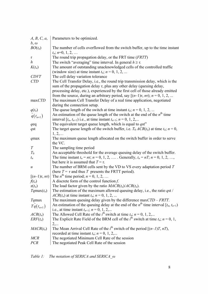
A, B, C, a, b, ω

Parameters to be optimized.

BO(tn) The number of cells overflowed from the switch buffer, up to the time instant tn; n=0, 1, 2, …

τ The round trip propagation delay, or the FRT time (FRTT) h The switch “averaging” time interval. In general h τ. K(tn) The amount of outstanding unacknowledged cells of the controlled traffic

(window size) at time instant tn; n = 0, 1, 2, ... CDVT The cell delay variation tolerance CTD The Cell Transfer Delay, i.e., the round trip transmission delay, which is the

sum of the propagation delay τ, plus any other delay (queuing delay, processing delay, etc.), experienced by the first cell of those already emitted from the source, during an arbitrary period, say [(n–1)τ, nτ); n = 0, 1, 2, ...

maxCTD The maximum Cell Transfer Delay of a real time application, negotiated during the connection setup.

q(tn) The queue length of the switch at time instant tn; n = 0, 1, 2, ...

1nq t An estimation of the queue length of the switch at the end of the nth time

interval [tn, tn+1) i.e., at time instant tn+1; n = 0, 1, 2,... qeq The equivalent target queue length, which is equal to qstω qst The target queue length of the switch buffer, i.e. T0 ACR(tn) at time tn; n = 0,

1, 2,… qmax The maximum queue length allocated on the switch buffer in order to serve

the VC. T The sampling time period T0 An acceptable threshold for the average queuing delay of the switch buffer. tn The time instant tn = nτ; n = 0, 1, 2, …. . Generally, tn = nT; n = 0, 1, 2, …,

but here it is assumed that T = τ. u The number of BRM cells sent by the VD to VS every adaptation period T

(here T = τ and thus T presents the FRTT period). [(n–1)τ, nτ) The nth time period; n = 0, 1, 2, … f(tn) A discrete form of the control function f. z(tn) The load factor given by the ratio MACR(tn)/ACR(tn). Tqmax(tn) The estimation of the maximum allowed queuing delay, i.e., the ratio qst /

ACR(tn) at time instant tn; n = 0, 1, 2, ... Tqmax The maximum queuing delay given by the difference maxCTD – FRTT.

1nT q t An estimation of the queuing delay at the end of the nth time interval [tn, tn+1)

i.e., at time instant tn+1; n = 0, 1, 2,... ACR(tn) The Allowed Cell Rate of the ith switch at time tn; n = 0, 1, 2,... ERF(tn) The Explicit Rate Field of the BRM cell of the ith switch at time tn; n = 0, 1,

2,... MACR(tn) The Mean Arrival Cell Rate of the ith switch of the period [(n–1)T, nT),

recorded at time instant tn; n = 0, 1, 2,... MCR The negotiated Minimum Cell Rate of the session PCR The negotiated Peak Cell Rate of the session

Table 1: The notation of SERICA and SERICA_ω

9

Tqmax(tn) = qmax / ACR(tn) ≤ Tqmax = qmax / MCR is the estimation of the maximum allowed queuing delay of the current time instant tn.

T0 = h [PCR + MCR – ACR(tn)] / ACR(tn) presents the target queuing delay of the switch. Note that in case of the ABR service T0 = CDVT, whereas in case of the extended ABR service, T0 = maxCTD – τ.

As it has been pointed out the SERICA algorithm, attempts to obtain the most

throughput. This has been achieved by adjusting the VS emission rate and the VD buffer occupancy in accordance with the ACR and the qst respectively. The algorithm is able to guarantee a specific SCR according to the traffic descriptor set of the session. Thus, the network is able to support real and/or non-real time traffic over ABR, such as the Diff Serv applications. However, SERICA is not able to face a particular problem of a NSP, related with the availability of the buffer resources. For example, a new client would not be able to merit the negotiated service on call due to the low availability of the switch buffer. Thus, this client would prefer to join a session with less guaranteed throughput, than nothing.

From the above it appears that a new ER-based switch algorithm is required, be means of the SERICA_ω scheme, which in general will be able to support a target queuing delay lower than (or at most equal to) the T0 proposed by the SERICA algorithm. This new scheme will be used as a “gearbox”, to initialize a session according to the buffer availability. Into this context the parameter ω plays the role of the “gear ratio” used.

3. THE SERICA_ω ALGORITHM 3.1. Model Analysis As it has been pointed out, the values given by the floater control mechanism are approximated through a suitable control function. This function regulates the traffic flow and keeps the queue length values less than the target queue length qst, namely the threshold provided by the SERICA algorithm. This is an interesting problem since it corresponds in the case in which the network administrator may not be able to establish a session due to the low buffer availability. Figure 4 depicts graphically various possibilities to regulate the traffic flow, by considering some well-known mechanical examples.

To keep the equations used as simple as possible, the mathematical description of the window K(tn) given by equation (1) should not be changed. However to increase the flexibility of the system, by means of establishing a session with target queue length lower than the threshold qst provided by the SERICA algorithm, the source window variation ΔK(tn) is assumed to scale arbitrarily. From the administrator point of view this approach appears to be simple and efficient, nevertheless, as it will be seen later, it increases the instability of the system.

Beholding that ΔK(tn) depends on the unpredictably varied parameter ACR of the switch, an unpredictable growth of the queue length may be observed at the switch buffer. Of course, this may result in cell losses, either due to overflow, or due to the non-conformance test. As an example, we may consider the case of processing a long file

10

transfer, during which it is desired to avoid congestion by keeping cell loss closed to zero. A solution in such problems may be obtained through an Explicit Rate switch algorithm, in which the source window variation ΔK(tn) is assumed to be approximated generally by a polynomial function of order ω of the queue length of the switch, acknowledged at the source at time tn. Thus, in a steady state, i.e. when ACR remains constant and in case the observer is located in the VS site, ΔK(tn) may assumed to be of the form:

1 10 1 0 1 1 0 1 1 0Δ ...ω ω

n n n ω n ωK t A q t τ A q t τ A q t τ A (3)

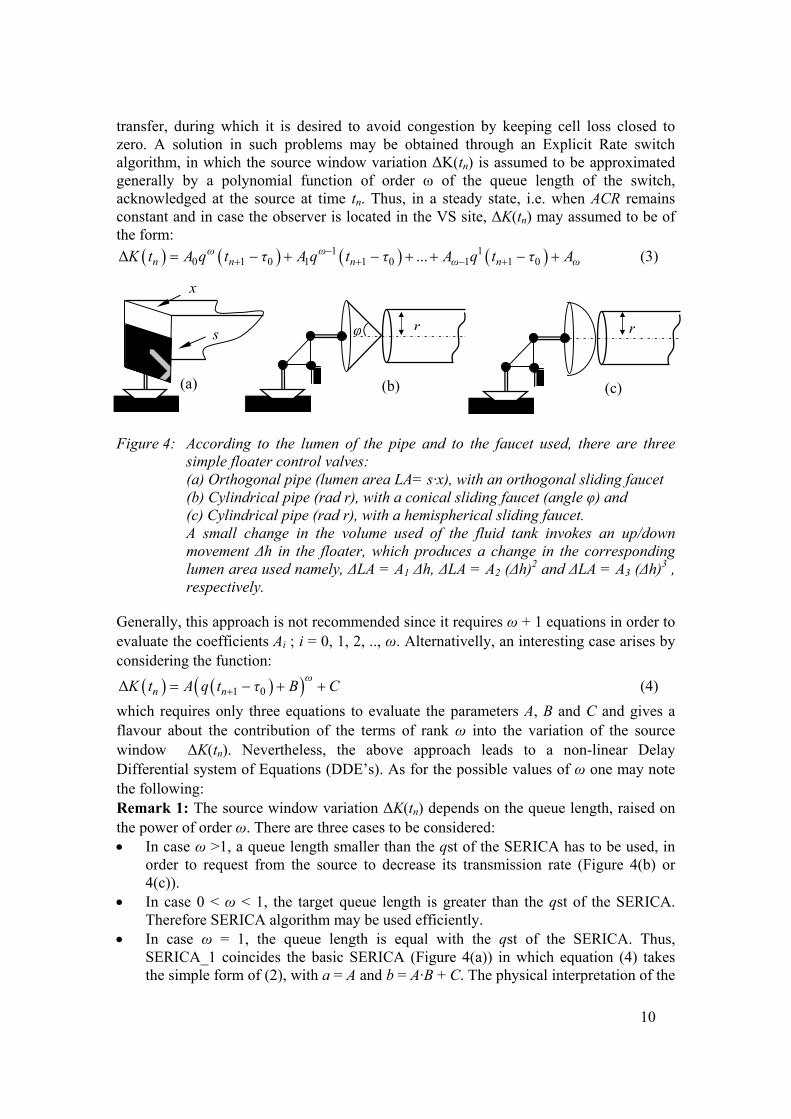
Figure 4: According to the lumen of the pipe and to the faucet used, there are three

simple floater control valves: (a) Orthogonal pipe (lumen area LA= s·x), with an orthogonal sliding faucet (b) Cylindrical pipe (rad r), with a conical sliding faucet (angle φ) and (c) Cylindrical pipe (rad r), with a hemispherical sliding faucet. A small change in the volume used of the fluid tank invokes an up/down

movement Δh in the floater, which produces a change in the corresponding lumen area used namely, ΔLA = A1 Δh, ΔLA = A2 (Δh)2 and ΔLA = A3 (Δh)3 , respectively.

Generally, this approach is not recommended since it requires ω + 1 equations in order to evaluate the coefficients Ai ; i = 0, 1, 2, .., ω. Alternativelly, an interesting case arises by considering the function:

1 0Δω

n nK t A q t τ B C (4)

which requires only three equations to evaluate the parameters A, B and C and gives a flavour about the contribution of the terms of rank ω into the variation of the source window ΔK(tn). Nevertheless, the above approach leads to a non-linear Delay Differential system of Equations (DDE’s). As for the possible values of ω one may note the following: Remark 1: The source window variation ΔK(tn) depends on the queue length, raised on the power of order ω. There are three cases to be considered: In case ω >1, a queue length smaller than the qst of the SERICA has to be used, in

order to request from the source to decrease its transmission rate (Figure 4(b) or 4(c)).

In case 0 < ω < 1, the target queue length is greater than the qst of the SERICA. Therefore SERICA algorithm may be used efficiently.

In case ω = 1, the queue length is equal with the qst of the SERICA. Thus, SERICA_1 coincides the basic SERICA (Figure 4(a)) in which equation (4) takes the simple form of (2), with a = A and b = A·B + C. The physical interpretation of the

rφ

(b)

r

(c) (a)

s

x

11

equation (2) is that when q(tn+1) is approximated with – b/a the window will not change, namely, K(tn+1) = K(tn). In this case MACR(tn+1) = MACR(tn) = ACR(tn), which verifies that (q(tn+1), MACR(tn+1)) = (– b/a, ACR(tn)) is an equilibrium point. SERICA_1 has been fully examined in Mousadis & Tsiligirides (2002).

3.2. Numerical Analysis The analysis for the case of interest (ω > 1) starts by eliminating the source window parameter K(tn). This may be achieved by using equations (1) and (4) above. Thus, by differentiating the equation (1) above, one may obtain:

0 0n n nd d d

K t τ MACR t τ q t τdt dt dt

The first derivative of K(tn) is calculated from equation (4) as follows:

01 0

Δ

Δ

ωn nn n

K t ACR t τdK t A q t τ B C

dt t u

; Δt = u / ACR(tn–τ0),

Therefore, in case of A 0:

00 1 0 0

ω nn n n

q t τd C A dMACR t τ q t τ B ACR t τ

dt A uτ dt τ

.

Similarly, assuming the observer is located in the VD site, it follows:

1

ω nn n n

q td C A dMACR t q t B ACR t

dt A uτ dt τ

.

The non-linear system of ODEs that combines the rate of the VS with the queue

length of the switch at time tn is given by the following system of equations:

1

, if (a)

, if (b)

max , if (c)

ωn

ω nn n n

ωn

CB ACR t

uτq td C A d

MACR t q t B ACR tdt A uτ dt τ

C Aq B ACR t

A uτ

(5)

and

, if (b)

0, otherwise (i.e., (a) & (c))

n nn

MACR t ACR tdq t

dt (6)

where:

(a) 0 n n nq t MACR t ACR t

0 max , or

(b) 0 , or

max

n

n n n

n n n

q t q

q t MACR t ACR t

q t q MACR t ACR t

12

(c) max n n nq t q MACR t ACR t

In the above, qmax = PCR (maxCTD – τ) = (PCR – MCR) CDVT + PCR·T0 is the maximum

threshold of the queue length of the switch q(tn+1) is estimated through the first derivative of the queue length at time tn, using

the Euler method. Thus,

1

, if (b)

, otherwise

n n nn

n

q t MACR t ACR t τq t

q t

According to the operational environment determined by the parameters MACR, ACR and queue length at the switch, the system of equations (5) and (6) should lead automatically in a stable focus point, which provides a “safe life” for the session. Provided that the above system has only one equilibrium point, the corresponding root must be real and positive, whereas all the remaining should be conjugate complex, or negative. The desired root is given by (MACR, q) = (ACR, qst). Note that in the above analysis we exclude the case of ACR = 0 and / or MACR = 0, which leads to the trivial case of (MACR, q) = (0, 0). In addition;

0, if (a)

0, if st

0, if st

0, if st

0, if (c)

n

n n

n

q t qd

MACR t q t qdt

q t q

or,

, if (a)

, if st

, if st

, if st

, if (c)

n

n n n

n

q t q

MACR t MACR t q t q

q t q

and the system remains closed to the equilibrium point (ACR, qst). Note that the parameter values for MACR and ACR change at any time instant tn; n = 0, 1, 2, ... and therefore different values of ACR(tn) determine different equilibria points. However, since ACR(tn) varies unpredictably between two consecutive time instants, the system will be considered in a steady state condition, i.e., the ACR(tn) remains constant for more than one averaging time interval.

In order to determine the target queue length of the switch buffer qst, we assume A =

– uτ/ACR(tn). Note that in the following and for simplicity reasons we will denote by qst, instead of qst(ACR(tn)).Thus, qst := – B + (– C/A)1/ω = – B + (C·ACR(tn)/(uτ))

1/ω .

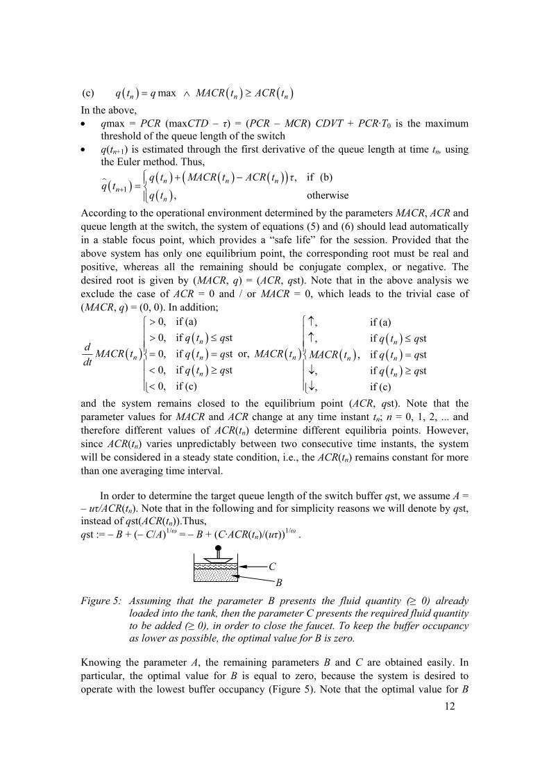
Figure 5: Assuming that the parameter B presents the fluid quantity (≥ 0) already loaded into the tank, then the parameter C presents the required fluid quantity to be added (≥ 0), in order to close the faucet. To keep the buffer occupancy as lower as possible, the optimal value for B is zero.

Knowing the parameter A, the remaining parameters B and C are obtained easily. In particular, the optimal value for B is equal to zero, because the system is desired to operate with the lowest buffer occupancy (Figure 5). Note that the optimal value for B

B

C

13

determines the target queue length of the switch buffer as:

qst := (– C/A)1/ω = 1/ω

nACR tC

uτ

.

Finally, assuming that the target queuing delay, T0 say, is specified by the application being in service, qst = T0 ACR(tn) and therefore, C = T0 u τ (ACR(tn))

(ω-1)/ω. As it appears, for large values of ω, the ratio (ω – 1)/ω →1 and hence the parameter C → T0 u τ ACR(tn), which implies that qst → (T0ACR2)1/ω → 1. However the values of ω > 1 increase the instability of the system, namely, it causes an oscillating behavior around the equilibrium point (Figure 6(b)). Hence, small values of ω are more important (Figure 6(a)). Note that Figure 4 shows some interesting particular cases of the floater control valve, in which a faucet with different geometry may change dramatically the fluid quantity required to close the pipe. Thus, small values of ω decrease the queuing delay.

Given the traffic descriptor, the NSP will serve a client, in the worst case, in accordance with the negotiated target queuing delay (here the worst case is presented with the SERICA_1 algorithm). Hence, parameter T0 is derived as: T0 = [h (PCR + MCR – ACR(tn))]

1/ω / ACR(tn). and acknowledges that SERICA_ω algorithm always use auto-adjusted parameters, to achieve in the worst case a target queuing delay, related with the selected value of ω, as well as, with the negotiated traffic descriptor set for PCR and MCR. Taking into account the values for B and qst the system of ODEs described by equations (5) and (6) may be rewritten as follows:

1

st , if (a)

st , if (b)

max st , if (c)

ω

ω nωn n

ω ω

q

q td dMACR t q t q

dt dt τ

q q

(7)

, if (b)

0, otherwisen n

nMACR t ACR td

q tdt

(8)

The above system is solved numerically using the Euler method with step h = τ . Note that the parameter ACR is assumed to remain fixed at least for a period equal to h and that generally h ≥ τ. In the WCT, namely when the source is able to transmit at the requested rate:

n nd

MACR t h MACR tdt

= MACR(tn+1) = ERF(tn)

By integrating equation (7), with step h, one may obtain :

1

st , if (a)

st , if (b)

max st , if (c)

ω

ω ωn n n n

ω ω

q h

h dERF t MACR t q t q h q t

τ dt

q q h

(9)

14

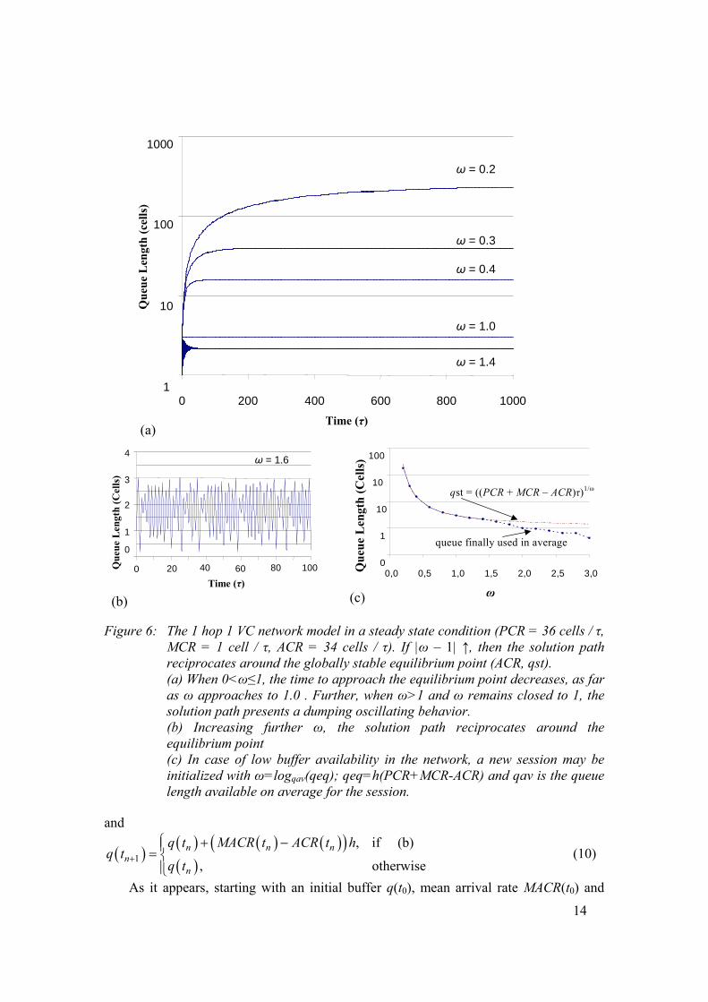
Figure 6: The 1 hop 1 VC network model in a steady state condition (PCR = 36 cells / τ, MCR = 1 cell / τ, ACR = 34 cells / τ). If |ω – 1| ↑, then the solution path reciprocates around the globally stable equilibrium point (ACR, qst).

(a) When 0<ω≤1, the time to approach the equilibrium point decreases, as far as ω approaches to 1.0 . Further, when ω>1 and ω remains closed to 1, the solution path presents a dumping oscillating behavior.

(b) Increasing further ω, the solution path reciprocates around the equilibrium point

(c) In case of low buffer availability in the network, a new session may be initialized with ω=logqav(qeq); qeq=h(PCR+MCR-ACR) and qav is the queue length available on average for the session.

and

1

, if (b)

, otherwise

n n nn

n

q t MACR t ACR t hq t

q t

(10)

As it appears, starting with an initial buffer q(t0), mean arrival rate MACR(t0) and

1

10

100

1000

0 200 400 600 800 1000

Time (τ)

Qu

eue

Len

gth

(ce

lls)

ω = 0.2

ω = 0.3

ω = 0.4

ω = 1.0

ω = 1.4

(a)

0

1

2

3

4

0 20 40 60 80 100 Time (τ)

Qu

eue

Len

gth

(C

ells

)

ω = 1.6

(b)

0

1

10

10

100

0,0 0,5 1,0 1,5 2,0 2,5 3,0

ω

Qu

eue

Len

gth

(C

ells

)

qst = ((PCR + MCR – ACR)τ)1/ω

queue finally used in average

(c)

15

allowed cell rate ACR(t0), the procedure enables the calculation of the MACR(t1) (= ERF(t0)) from equation (9), using the Euler method. This value is used to calculate the

new buffer q(t1) estimated by 1q t ), which is then used to produce the new MACR(t2) (=

ERF(t1)) and so on. Note that the switch sends u BRM cells every time period τ keeping the same ERF value, because the corresponding ACR(tn) is assumed constant during the time period [nτ, (n+1)τ).

Clearly, the number of cells exceeding qmax, say BO(tn), varies with rate given by:

, if max

0, otherwisen n n n n

nMACR t ACR t q t q MACR t ACR td

BO tdt

(11)

The function f(q(tn)) is derived in a straight-forward manner as:

0

0 1 1

0 1

, if (a)

_ , st, , if (b)

max , st, , if (c)

ωn

n n n n

n n

z t hT

τ h hf ω t z t h T T q t φ q t q ω

τ τ

z t h T T φ q t q ω

In the above: z(tn) = MACR(tn) / ACR(tn) denotes the load factor at time tn.

1nT q t = 1nq t

/ ACR(tn) denotes an estimation for the queuing delay at the end

of the nth time instant [tn, tn+1) i.e., at time tn+1; tn+1 = tn + h. Tqmax(tn) = qmax / ACR(tn) ≤ Tqmax = qmax / MCR is the estimation of the

maximum allowed queuing delay of the current time instant tn.

11

1

st, st,

st

ωωn

n

n

q q tφ q t q ω

q q t

As we shall see, the above function f_ω(tn) will be simplified further, in accordance with the actual value taken of the parameter ω.

Thus, the new session will start with the SERICA_ω (e.g., with ω = 2) algorithm. When the buffer availability increases (i.e., when more memory may be allocated to this session), the system toggles the algorithm from the SERICA_ω, to the SERICA_1. I.e., the new session will start with a “gear ratio” ω >1 in the “gearbox” of SERICA. The key point of SERICA_ω algorithm is that it may be used in order to achieve lower values of queue length than the qst of the SERICA algorithm, which at least resides in the order of O(PCR1/ω). Thus, the SERICA_ω algorithm may be used to operate with a small available queue threshold at the switch. Further, one may configure the qmax =(2 PCR h)1/ω in order to serve most of the users.

3.3. Stability analysis Usually it is very hard to determine the domain of stability of an equilibrium point. Rigorous mathematical definitions are often too prescriptive and it is not always clear wich properties of solutions or equations are most important in the context of any particular problem. In practice, different definitions are used according to the problem

16

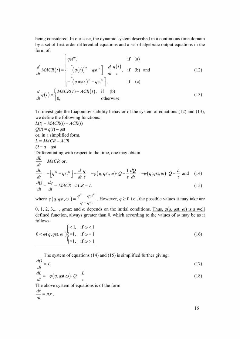
being considered. In our case, the dynamic system described in a continuous time domain by a set of first order differential equations and a set of algebraic output equations in the form of:

st , if (a)

st , if (b)

max st , if (c)

ω

ω ω

ω ω

q

q td dMACR t q t q

dt dt τ

q q

and (12)

, if (b)

0, otherwise

MACR t ACR tdq t

dt

(13)

To investigate the Liapounov stability behavior of the system of equations (12) and (13), we define the following functions: L(t) = MACR(t) – ACR(t) Q(t) = q(t) – qst or, in a simplified form, L = MACR – ACR Q = q – qst Differentiating with respect to the time, one may obtain dL

MACRdt

or,

1st , st, , st,

ω ωdL d q dQ Lq q φ q q ω Q φ q q ω Q

dt dt τ τ dt τ and (14)

-dQ dq

MACR ACR Ldt dt

(15)

where ωst

, st, st

ωq qφ q q ω

q q

. However, q 0 i.e., the possible values it may take are

0, 1, 2, 3,... , qmax and ω depends on the initial conditions. Thus, φ(q, qst, ω) is a well defined function, always greater than 0, which according to the values of ω may be as it follows:

1, if 1

0 , st, =1, if 1

>1, if 1

ω

φ q q ω ω

ω

(16)

The system of equations (14) and (15) is simplified further giving:

dQL

dt (17)

, st, dL L

φ q q ω Qdt τ

(18)

The above system of equations is of the form

Adx

xdt

,

17

where

dLdx dt

dQdt

dt

, 0 1

A 1

φ

τ

and

Lx

Q; φ = φ(q, qst, ω).

In the above, A is a Jacobian matrix and for simplicity we assume that τ = 1. Looking for

equilibrium points with 0dL

dt and 0

dQ

dt we see that (L, Q) = (0, 0). The

characteristic equation of the above system is |sI-A| = 0, or, s(s+1)+φ = 0, or, s2 + s + φ = 0 (19)

Hence, the eigenvalues of A, are:

1,2

1 1 4

2

φs

1 4 1

2

i φ

Both of them have strictly negative real parts for all φ > 1/4 presenting the boundary values between of which the solution path is to oscillate. Provided that 1-4φ ≠ 0, or, φ ≠ 1/4, they are distinct. Therefore, the equilibrium point (0, 0) is asymptotically stable (Figure 6).

To present the stability behavior of the system under consideration, some indicative

values for ω are examined, namely ω = 1, (SERICA_1 – gear ratio 1), ω = 2 (SERICA_2 – gear ratio 2) and ω = 3 (SERICA_3 – gear ratio 3), which correspond to φ(q, qst, ω) =1, φ(q, qst, ω) = q + qst and φ(q, qst, ω) = q2 + q·qst + qst2 respectively and are all greater than, or equal to 1. Thus, the equilibrium point (0, 0) is asymptotically stable for each one of the above cases.

4. SIMULATION RESULTS SERICA_ω introduces a series of similar algorithms according to the different values of ω. Nevertheless, the most useful members of this family appears to be: SERICA_1 because it works as the basic SERICA algorithm and SERICA_2, because its target queue length is the square root of the one referred to

the SERICA_1. For example, a switch operating with the SERICA_2 algorithm will use, in average, less than or equal to 50% of the buffer allocated to the SERICA_1 algorithm.

In the following the SERICA_2 is tested by simulation using the simple configuration shown in Figure 7. This network configuration consists of a source, two ABR switches and a destination, connected in tandem using a single VC. The ABR traffic descriptor parameters are: PCR = 36 cells/τ, MCR = 1 cell/τ and qmax = 2 h PCR, with h = τ = 1. The simulator used herein, is the same as the one described by Mousadis & Tsiligirides (2002) and it is used to produce extended simulation results, over a period of 1000τ, according to the ATM FORUM (1996), “Performance Testing Spec.”.

Source Switch 2 DestinationSwitch 1

Figure 7: The 2 hop, 1 VC network model.

18

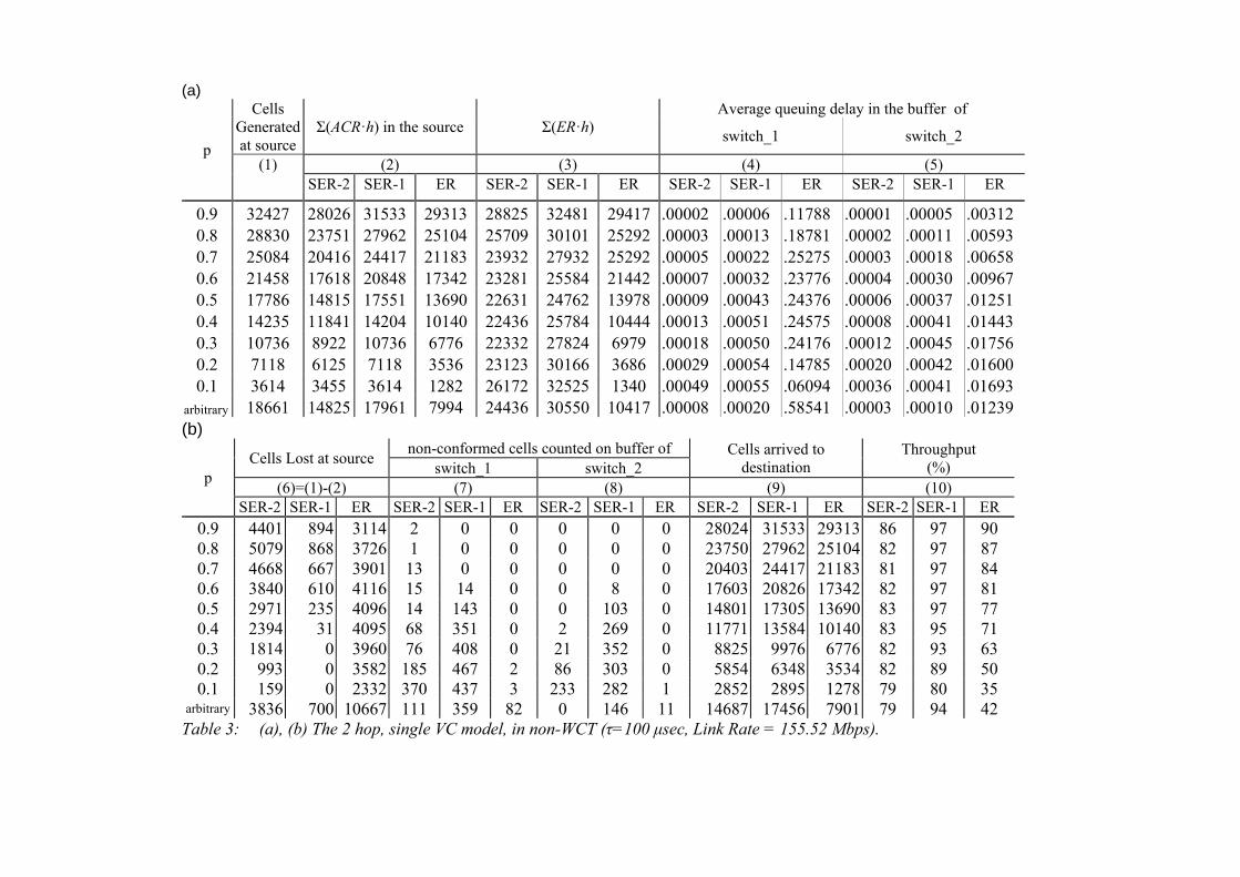
The SERICA_2 algorithm is tested versus the SERICA_1 and the ERICA/ERICA+ scheme, using the same simulation environment of Mousadis & Tsiligirides (2002). The simulation results are presented in Table 2 (a) and (b). The description of Table 2(a) is beginning by showing in column “p” the corresponding probability values, used to generate a number of cells at the source, presented in the column (1). These cells will be transmitted through the network, using the three ER-based congestion avoidance algorithms, denoted in the columns of Table 2 as ‘SER-2’, ‘SER-1’ and ‘ER’, respectively. Column (2) shows the actual number of cells transmitted in each session, while column (3) presents the number of cells requested by the source during the same session. The average queuing delay in the buffer of the switches 1 and 2 are shown in columns (4) and (5) respectively. Further, in Table 2(b), in column (6) are shown the number of cells waiting in the source to be transmitted, when the time slot expires. These cells will never be transmitted and therefore they are discarded from the queue, namely they are considered as lost. This assumption may help in a theoretical analysis of the model and it is not harmful in real applications. The cells that finally arrived at the destination are shown in column (9). Further, in columns (7) and (8) is presented the number of cells taken away from the buffer queues of the switches 1 and 2 respectively, since their lifetime (CDVT) of 2τ has been expired. Finally, in column (10) the throughput of each session is presented in a per % scale. As it appears from the simulation, the overflow rate BO(tn) given by the equation (11) is zero for all of the tested algorithms and thus it is excluded from this table.

The simulation shows some interesting results concerning the overall performance of the SERICA_ω algorithms versus the ERICA/ERICA+ algorithm, by means of the higher throughput achieved. In particular, as one may observe, SERICA_1 gives always better throughput than SERICA_2 and ERICA. Note that: SERICA_2 achieves better throughput than the ERICA/ERICA+ in cases where p

takes moderate values. Overall, using SERICA_ω the throughput achieved is always more than 79%.

In case the probability p is “arbitrary”, (namely, p varies from slot to slot during a session)SERICA_1 performs better than SERICA_2, whereas SERICA_2 performs better than ERICA/ERICA+. This case may correspond to the unpredictable ABR traffic environment, in which sudden changes of the input rate in the source causes unexpected behavior in the system performance.

In terms of the queue length, or of the queuing delay, SERICA_2 seems to achieve very low values for all p.

Although SERICA_1 is always better than SERICA_2, in terms of throughput, there are cases where SERICA_2 should be preferred, particularly when the buffer availability is low and a new session is to be established

(a) Average queuing delay in the buffer of Cells

Generated at source

Σ(ACR·h) in the source Σ(ER·h) switch_1 switch_2

(2) (3) (4) (5) p

(1) SER-2 SER-1 ER SER-2 SER-1 ER SER-2 SER-1 ER SER-2 SER-1 ER

0.9 32427 28026 31533 29313 28825 32481 29417 .00002 .00006 .11788 .00001 .00005 .00312 0.8 28830 23751 27962 25104 25709 30101 25292 .00003 .00013 .18781 .00002 .00011 .00593 0.7 25084 20416 24417 21183 23932 27932 25292 .00005 .00022 .25275 .00003 .00018 .00658 0.6 21458 17618 20848 17342 23281 25584 21442 .00007 .00032 .23776 .00004 .00030 .00967 0.5 17786 14815 17551 13690 22631 24762 13978 .00009 .00043 .24376 .00006 .00037 .01251 0.4 14235 11841 14204 10140 22436 25784 10444 .00013 .00051 .24575 .00008 .00041 .01443 0.3 10736 8922 10736 6776 22332 27824 6979 .00018 .00050 .24176 .00012 .00045 .01756 0.2 7118 6125 7118 3536 23123 30166 3686 .00029 .00054 .14785 .00020 .00042 .01600 0.1 3614 3455 3614 1282 26172 32525 1340 .00049 .00055 .06094 .00036 .00041 .01693

arbitrary 18661 14825 17961 7994 24436 30550 10417 .00008 .00020 .58541 .00003 .00010 .01239 (b)

non-conformed cells counted on buffer of Cells Lost at source

switch_1 switch_2 Cells arrived to

destination Throughput

(%) (6)=(1)-(2) (7) (8) (9) (10)

p

SER-2 SER-1 ER SER-2 SER-1 ER SER-2 SER-1 ER SER-2 SER-1 ER SER-2 SER-1 ER

0.9 4401 894 3114 2 0 0 0 0 0 28024 31533 29313 86 97 90 0.8 5079 868 3726 1 0 0 0 0 0 23750 27962 25104 82 97 87 0.7 4668 667 3901 13 0 0 0 0 0 20403 24417 21183 81 97 84 0.6 3840 610 4116 15 14 0 0 8 0 17603 20826 17342 82 97 81 0.5 2971 235 4096 14 143 0 0 103 0 14801 17305 13690 83 97 77 0.4 2394 31 4095 68 351 0 2 269 0 11771 13584 10140 83 95 71 0.3 1814 0 3960 76 408 0 21 352 0 8825 9976 6776 82 93 63 0.2 993 0 3582 185 467 2 86 303 0 5854 6348 3534 82 89 50 0.1 159 0 2332 370 437 3 233 282 1 2852 2895 1278 79 80 35

arbitrary 3836 700 10667 111 359 82 0 146 11 14687 17456 7901 79 94 42 Table 3: (a), (b) The 2 hop, single VC model, in non-WCT (τ=100 μsec, Link Rate = 155.52 Mbps).

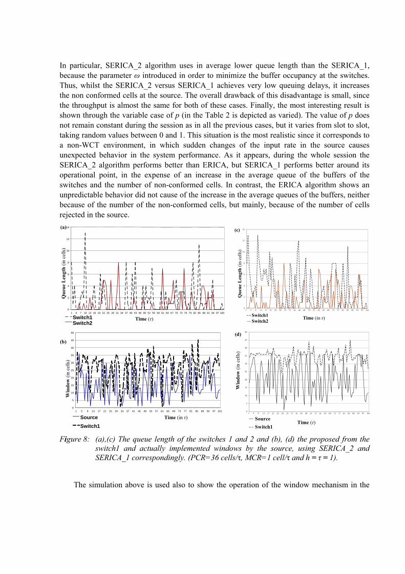
In particular, SERICA_2 algorithm uses in average lower queue length than the SERICA_1, because the parameter ω introduced in order to minimize the buffer occupancy at the switches. Thus, whilst the SERICA_2 versus SERICA_1 achieves very low queuing delays, it increases the non conformed cells at the source. The overall drawback of this disadvantage is small, since the throughput is almost the same for both of these cases. Finally, the most interesting result is shown through the variable case of p (in the Table 2 is depicted as varied). The value of p does not remain constant during the session as in all the previous cases, but it varies from slot to slot, taking random values between 0 and 1. This situation is the most realistic since it corresponds to a non-WCT environment, in which sudden changes of the input rate in the source causes unexpected behavior in the system performance. As it appears, during the whole session the SERICA_2 algorithm performs better than ERICA, but SERICA_1 performs better around its operational point, in the expense of an increase in the average queue of the buffers of the switches and the number of non-conformed cells. In contrast, the ERICA algorithm shows an unpredictable behavior did not cause of the increase in the average queues of the buffers, neither because of the number of the non-conformed cells, but mainly, because of the number of cells rejected in the source.

Figure 8: (a),(c) The queue length of the switches 1 and 2 and (b), (d) the proposed from the switch1 and actually implemented windows by the source, using SERICA_2 and SERICA_1 correspondingly. (PCR=36 cells/τ, MCR=1 cell/τ and h = τ = 1).

The simulation above is used also to show the operation of the window mechanism in the

0

2

4

6

8

10

12

14

1 5 9 13 17 21 25 29 33 37 41 45 49 53 57 61 65 69 73 77 81 85 89 93 97 101

Time (in τ)

Qu

eue

Len

gth

(in

cel

ls)

Switch1Switch2

(c)

0

5

10

15

20

25

30

35

40

45

50

1 5 9 13 17 21 25 29 33 37 41 45 49 53 57 61 65 69 73 77 81 85 89 93 97 101

Time (τ)

Win

dow

(in

cel

ls)

Source

Switch1

(d)

0 2 4 6 8

10 12 14

1 4 7 10 13 16 19 22 25 28 31 34 37 40 43 46 49 52 55 58 61 64 67 70 73 76 79 82 85 88 91 94 97 100

Time (τ)

Qu

eue

Len

gth

(in

cel

ls)

Switch1 Switch2

(a)

0 5

10 15 20 25 30 35 40 45 50

1 5 9 13 17 21 25 29 33 37 41 45 49 53 57 61 65 69 73 77 81 85 89 93 97 101

Time (in τ)

Win

dow

(in

cel

ls)

Source

Switch1

(b)

21

network configuration of Figure 7. The results produced using the SERICA_2 and the SERICA_1, are depicted in Figure 8 (cases a, c and b, d respectively). Figures 8a and 8c show that using the SERICA_2, the queue length (in cells) of each of the switches 1 and 2 over the time is lower in average than that using the SERICA_1. Further, Figures 8b and 8d show the window (in cells), as it is proposed from the switch 1 to be implemented by the source, as well as the window actually implemented by the source. As one may see, the proposed window of the switch 1 via the SERICA_2 presents the expected bigger amplitude (corresponded to the φ(qprn, qst) for ω = 2) in the window, than that produced using the SERICA_1 .

5. CONCLUSIONS

In this work we extended the SERICA and derived the SERICA_ω scheme. This new scheme examined through simulation to regulate the flow of the ABR traffic in an ATM network. SERICA_ω derivation is based on a network configuration consisted of M switches in tandem, with multiple VCs, allowing the VS/VD property. The analysis used a hop-by-hop strategy in which the cross traffic immediately leaves the switch.

SERICA_ω was developed to dynamically adjust the VS window size, by regulating its emission rate, through the ERF of the BRM cells sent from the VD. The ACR, MACR, and q were modeled as fluids and as a result the discrete model was presented as a non-linear system of ODEs. Thus, for every case of ω and in steady state it is totally stable. The above system of ODEs was solved using a simple numerical method. Derivation of the appropriate family f(q) for the SERICA_ω was left for the future.

Extended simulation results on a simple network configuration proved the robustness of the new scheme i.e., that the achieved throughput has always been greater than 79% of the initially generated cells at the source and that the queuing delay has been minimized, in the unpredictably varied ABR environment, as well as, in the predictable VBR environment. The most important is that the new scheme may be used from the network administrator as a “gear box” to initialize a new session with a low buffer availability and then to serve the session in a “safe life” operating procedure.

REFERENCES 1. Arnold V. I. (1978), “Ordinary Differential Equations”, in Arnold V. I. (ed.) MIT Press edition, ISBN 0-262-51018-9. 2. ATM FORUM (1996), “Traffic Management Spec. V. 4.0”. ftp://ftp.atmforum.com/pub/ approved-specs/af-tm-0056.000.ps, April 1996. 3. ATM FORUM (1996), “Performance Testing Spec.”. 11-30-96 5:42 AM, ATM Forum/BTD-TEST-TM-PERF.00.00(96-0810R3), http://www.cis.ohio-state.edu/~jain/ atmforum.htm 4. FUJITSU (2000), “Real Time Cell Flow Processing TM”, A White Paper, http://www.nexen.com/new_web/ wprealtime.html. 5. Jain R., Kalyanaraman S., Goyal R., Fahmy S. and Fang Lu (1995), “ERICA+: Extensions to the ERICA switch algorithm”, ATM Forum/95/1346, Oct. 1995. 6. Kalyanaraman S. (1997), “Traffic Management for the Available Bit Rate (ABR) Service in Asynchronous Transfer Mode (ATM) networks”, Ph. D. Dissertation, Dept. of Computer and Information Sciences, The Ohio State University, August 1997.

22

7. Kalyanaraman S., Jain R., Fahmy S., Goyal R., and Vandalore B. (2000), “The ERICA Switch Algorithm For ABR Traffic Management in ATM Networks”, IEEE/ACM Trans. Net.,8(1) (2000), pp. 87-98. 8. J. Mignault, A. Gravey and C. Rosenberg, (1996), "A survey of straightforward statistical multiplexing models for ATM networks", Telecomm.Sys. 5 (1996) pp.177-208. 9. Mousadis G., Tsiligirides T. and Bekakos M. (1996), Traffic Considerations for the Performance Evaluation of the ATM Networks, Proc. HERMIS-’96, pp. 289 – 299. 10. Mousadis G. (2001), “Flow Control Algorithms for the High Speed Computer Networks”, Ph. D. Dissertation, Dept. of General Sciences, Agricultural University of Athens, September 2001. 11. Mousadis G. and Tsiligirides T. (2002), “A Simple Explicit Rate Identification Congestion Avoidance (SERICA) algorithm to support some TCP Differentiated Services over the ABR traffic”, Com Com Journal, 2041 paper accept.