Sequentially Adaptive Bayesian Learning Algorithms for

Inference and Optimization

John Geweke and Garland Durham∗

October 2, 2017

Abstract

The sequentially adaptive Bayesian learning algorithm (SABL) builds on and ties

together ideas from sequential Monte Carlo and simulated annealing. The algorithm

can be used to simulate from Bayesian posterior distributions, using either data tem-

pering or power tempering, or for optimization. A key feature of SABL is that the

introduction of information is adaptive and controlled, ensuring that the algorithm per-

forms reliably and efficiently in a wide variety of applications with off-the-shelf settings,

minimizing the need for tedious tuning, tinkering, trial and error by users. The algo-

rithm is pleasingly parallel, and a Matlab toolbox implementing the algorithm is able

to make efficient use of massively parallel computing environments such as graphics

processing units (GPUs) with minimal user effort. This paper describes the algorithm,

provides theoretical foundations, applies the algorithm to Bayesian inference and opti-

mization problems illustrating key properties of its operation, and briefly describes the

open source software implementation.

1 Introduction

Sequentially adaptive Bayesian learning (SABL) is an algorithm that simulates draws re-

cursively from a finite sequence of distributions converging to a stated posterior distribution.

∗Geweke (jgeweke@uw.edu): Amazon, University of Washington, and Australian Centre of Excellencefor Mathematical and Statistical Frontiers (ACEMS). Durham (gbdurham@calpoly.edu): California Poly-technic State University. Research described here was largely completed while Geweke was at Universityof Technology Sydney (UTS). The Australian Research Council provided financial support through grantDP130103356 to UTS and through grant CD140100049 to ACEMS. At UTS Huaxin Xu, Bin Peng and SimonYin assisted with software development. We acknowledge useful discussions with William C. McCauslandand Bart Frischkecht in the course of developing SABL.

1

At each step the algorithm operates based on what has been learned through the previous

steps in such a way that the next iteration will be able to do the same: thus the algorithm

is adaptive. The evolution from one distribution to the next can be thought of as the in-

corporation of new information regarding the posterior distribution of interest, mimicking

Bayesian updating. The algorithm can be used for either Bayesian inference or optimization.

SABL addresses optimization by recasting it as a sequence of Bayesian inference problems.

The SABL algorithm builds on and ties together ideas that have been developed largely

independently in the literatures on Bayesian inference and optimization over the past three

decades. From optimization it is related to simulated annealing (Kirkpatrick et al. 1983;

Goffe et al. 1994) and genetic algorithms (Schwefel 1977; Baker 1985, 1987; Pelikan et

al. 1999). Key ideas underlying the application of sequential Monte Carlo (SMC) to the

problem of Bayesian inference date back to Gordon, Salmond and Smith (1993). The

application of these ideas to the problem of simulating from a static posterior distribution

goes back to Fearnhead (1998), Gilks and Berzuini (2001) and Chopin (2002, 2004).

While some of the key ideas underlying SABL go back several decades, SABL builds

on and extends this work, operationalizing the theory to provide a fully realized algorithm

that has been applied to a variety of real world problems and been found to perform reliably

and efficiently with a minimum of user interaction. This paper states the procedures in-

volved, derives their properties, and demonstrates their effectiveness. A complete and fully

documented implementation of the algorithm is provided in the form of a Matlab toolbox,

SABL.1.

SABL provides an integrated framework and software for posterior simulation, by

means of either data tempering or power tempering, as well as optimization. This pa-

per shows that power tempering, while less commonly used, has important advantages.

While the idea of applying SMC methods to optimization has appeared previously in the

literature (e.g., Del Moral at al. 2006; Zhou and Chen 2013), there has been little work in

developing the details and engineering required for reliable application. This paper provides

a theoretical framework and new results regarding convergence. At the level of precision

achieved by SABL, the effects of finite precision arithmetic inherent in digital computing

hardware become very apparent. We demonstrate some of the implications and provide a

new method for evaluating second derivatives of the objective function at the mode accu-

rately and at little cost. We also demonstrate application of this idea to computing the

Huber “sandwich” estimator, useful in maximum likelihood asymptotics.

One of the key features of SABL is that the introduction of information is adaptive and

1Throughout, SABL refers specifically to the software, whereas SABL refers to the algorithm. The soft-ware can be obtained at http://depts.washington.edu/savtech/help/software, as can the accompanyingSABL Handbook.

2

controlled. Adaptation is critical for any SMC algorithm for posterior simulation, and SABL

builds on and refines existing practice. The goal here is to minimize the need for tedious

tuning, tinkering, trial and error well documented in Creal (2007) and familiar to anyone

who has tried to use sequential particle filters or simulated annealing in real applications

(as opposed to textbook problems). SABL fully and automatically addresses issues like

the particle depletion problem in sequential particle filters and the temperature reduction

problem in simulated annealing.

When using simulation methods, it is important to have means to assess the numer-

ical precision and reliability of the results obtained. By breaking the sample of simulated

parameter draws into independent groups, SABL provides estimates of numerical standard

error and relative numerical efficiency at minimal cost in either computing time or user

effort (Durham and Geweke 2014a). The incorporation of a mutation phase in SMC goes

back to at least Gilks and Berzuini (2001). SABL uses a novel and effective technique based

on relative numerical efficiency to assess when the particles have become sufficiently mixed.

While Douc and Moulines (2008) provide results on consistency and asymptotic nor-

mality for non-adaptive SMC, there has been little progress toward a theory supporting

the kinds of adaptive algorithms that are actually used in practice and that are essential

to practical applications. Furthermore, the conditions relied upon by Douc and Moulines

(2008) are of a recursive nature that makes direct verification highly tedious, and the nota-

tion and framework within which the results are stated are likely to be highly opaque to the

typical intended SABL user. We restate the relevant results in a more transparent form and

in the specific context of SABL. We also provide conditions that can be easily verified and

demonstrate their close relationship to classical importance sampling. In addition, SABL

incorporates an innovative approach, first developed in Durham and Geweke (2014a), that

extends the results of Douc and Moulines (2008) to the adaptive algorithms needed for

usable implementations.

Another key feature of the SABL algorithm is that most of it is embarrassingly parallel,

making it well-suited for computing environments with multiple processors, especially the

inexpensive massively parallel platforms provided by graphics processing units (GPUs) but

also CPU environments with dozens of cores such as the Linux scientific computing clusters

that are available through most universities and cloud computing platforms. The observa-

tion that sequential particle filters have this property is not new, but exploitation of the

property is quite another matter, requiring that a host of technical issues be addressed, and

so far as we are aware there is no other implementation of the sequential particle filter that

does so as effectively as SABL. Since increasing parallelism has largely supplanted faster

execution on a single core as the route by which advances in computational performance

3

are likely to take place for the forseeable future, pleasingly parallel algorithms like SABL

will become increasingly important components of the technical infrastructure in statistics,

econometrics and economics. Yet the learning curve for working in such environments is

quite steep, witnessed in a number of published papers and failed attempts in large insti-

tutions like central banks. All of the important technical difficulties are solved in the SABL

software package, with the consequence that experienced researchers and programmers—for

example, anyone with moderate Matlab skills—can readily take advantage of the perfo-

mance benefits associated with massively parallel computing environments, especially GPU

computing.

Section 2 provides an outline of the SABL algorithm sufficient for the rest of the paper

and provides references to more complete and detailed discussions. Section 3 develops the

foundations of SABL in probability theory. Section 4 discusses issues related to the use of

SABL for optimization. Section 5 provides several detailed examples illustrating the use

of SABL for inference and optimization. Section 6 concludes. And proofs of propositions

appear in Section 7.

2 The SABL algorithm for Bayesian inference

Fundamental to SABL is the vector θ ∈ Θ ⊆ Rm, which is the parameter vector in Bayesian

inference and the maximand in optimization. All functions in this paper should be presumed

Lebesgue measurable on Θ. A function f (θ) : Θ → R is a kernel if f (θ) ≥ 0 ∀ θ ∈ Θ and∫Θ f (θ) dθ <∞.

Several functions are central to the algorithm and its application: The initial kernel

is k0 (θ) and p0 (θ) = k0 (θ) /∫

Θ k0 (θ) dθ is the initial probability density ; k∗ (θ) is the

incremental function; k (θ) = k0 (θ) k∗ (θ) is the target kernel and p (θ) = k (θ) /∫

Θ k (θ) dθ

is the target probability density ; g (θ):Θ→ R is the function of interest.

In problems of Bayesian inference π0 is the prior density, Π0 denotes the corresponding

distribution, and the initial probability density is p0 (θ) = π0 (θ). The incremental function

k∗ (θ) is proportional to the likelihood function,

p(y1:T | θ) =T∏t=1

p(yt | y1:t−1, θ), (1)

where ys:t denotes successive data ys, . . . , yt. The posterior density is π (θ), Π denotes the

corresponding distribution, and the target probability density is p (θ) = π (θ).

We require that∫

Θ k (θ) |g (θ)| dθ < ∞. The leading Bayesian inference problem ad-

4

dressed by SABL is to approximate the posterior mean

EΠ (g) = g =

∫Θg (θ)π (θ) dθ =

∫Θ g (θ) k (θ) dθ∫

Θ k (θ) dθ

and to assess the accuracy of this approximation by means of an associated numerical

standard error and central limit theorem. The goal is to do this in a computationally efficient

manner and with little need for problem-specific tuning and experimentation relative to

alternative approaches.

With alternative interpretations of k0 and k∗ SABL applies to optimization problems.

Section 4 returns to this topic.

2.1 Overview

When used for Bayesian inference SABL is a posterior simulator. It may be regarded as

belonging to a family of algorithms discussed in the statistics literature and variously known

as sequential Monte Carlo (filters, samplers), recursive Monte Carlo filters, or (sequential)

particle filters, and we refer to these collectively as sequential Monte Carlo (SMC) algo-

rithms. The literature is quite extensive with dozens of major contributors. Creal (2012) is

a useful survey, and for references most closely related to SABL see Durham and Geweke

(2014a). The mode of convergence in SMC algorithms is the size of the random sample

that represents the distribution of θ. The elements of this random sample are known as

particles.

For reasons explained shortly the particles in SABL are doubly-indexed, θjn (j =

1, . . . , J ; n = 1, . . . , N), and the mode of convergence is in N . As in all SMC algorithms, the

particles evolve over the course of the algorithm through a sequence of transformation cycles.

Index the cycles by ` and denote the particles at the end of cycle ` by θ(`)jn (` = 1, . . . , L). The

particles θ(0)jn are drawn independently from the prior distribution Π0. For each ` = 1, . . . , L

the transformation in cycle ` targets a distribution Π` with kernel density k(`). In the final

cycle ΠL = Π (equivalently, k(L) (θ) = k (θ)) so that the particles θ(L)jn represent the posterior

distribution. The progression from cycle `− 1 to cycle ` in SABL may be characterized as

the introduction of new information and the evolution of the particles from θ(`−1)jn to θ

(`)jn

reflects Bayesian updating.

Each cycle is comprised of three phases.

• Correction (C) phase: Gradually incorporate new information. When enough new

information has been added, stop and construct weights such that the weighted par-

ticles(θ

(`−1)jn , w

(`)jn

)reflect the updated kernel k(`)(θ).

5

• Selection (S) phase: Resample in proportion to the weights so that the unweighted

particles θ(`,0)jn reflect k(`)(θ).

• Mutation (M) phase: For each particle execute a series of Metropolis-Hastings steps

to generate θ(`,κ)jn (κ = 1, 2, . . . ). When the particles have become sufficently mixed,

stop and set θ(`)jn = θ

(`,κ)jn .

But, for the algorithm to be useable in practice, details are needed as to how each of

these steps is to be actually implemented. The choices made determine how efficiently the

algorithm will work, and indeed whether it will provide reliable results at all.

There are three key places where implementation details are important: (a) determi-

nation of how much new information to add before stopping the C phase and constructing

the intermediate kernels k(`); (b) choice of proposal density for the Metropolis-Hastings

steps; and (c) determination of the stopping point for Metropolis iterations. SABL specifies

choices for each of these that have been found to work well in practice. The software package

SABL defaults to these but users may override them with custom alternatives if desired.

A further issue is that practical considerations require that the operation of the algo-

rithm at each of these three key junctures rely upon information provided by the current set

of particles (that is, that the algorithm be adaptive). For example, the Metropolis-Hastings

proposal densities in SABL are Gaussian with variance equal to the appropriately scaled

sample variance of the current particles. However, theoretical results ensuring convergence

with adaptation are not available, although Del Moral et al. (2012) makes some progress

in this direction. Section 3.3 summarizes the solution of this problem presented in Durham

and Geweke (2014a).

The following three sections address the C, S and M phases, respectively, concentrating

primarily on the innovations in SABL but also discussing their embarrassingly parallel

character. Additional detail can be found in Durham and Geweke (2014a) and the SABL

Handbook.

2.2 The correction (C) phase

The correction phase determines the kernel k(`) and the implied particle weights w(`)jn =

w(`)(θ

(`−1)jn

)= k(`)

(θ

(`−1)jn

)/k(`−1)

(θ

(`−1)jn

)(j = 1, . . . , J ;n = 1, . . . , N). The weights are

those that would be used in importance sampling with target density kernel k(`) and source

density kernel k(`−1). The evaluation of these weights is embarrassingly parallel in the

particles θjn, of which there are typically many thousands. When SABL executes using one

or more GPUs each particle corresponds to a thread running on a single core of the GPU.

6

There are two principal approaches to constructing the intermediate kernels k(`).

Data tempering introduces information as new observations are added to the sample

over time. We can think of decomposing the likelihood function (1) as

p (y1:T | θ) =L∏`=1

p(yt`−1+1:t` | y1:t`−1

, θ)

for 0 = t0 < . . . < tL = T , motivating the sequence of kernels

k(`)(θ) = p0(θ)∏i=1

p(yti−1+1:ti | y1:ti−1 , θ

)∝ p (θ|y1:t`) (2)

and associated weight functions

w(`) (θ) = k(`) (θ) /k(`−1) (θ) = p(yt`−1+1:t` | y1:t`−1

, θ).

Although data tempering can be implemented by introducing only a single observation

in each cycle (i.e., t` = `, ` = 1, 2, . . . , T ), there is a potentially large increase in computa-

tional efficiency afforded by introducing several or many observations in each. A common

practice is to introduce observations one by one, each time using the corresponding weight

function

w(`)s (θ) = p

(yt`−1+1:t`−1+s | y1:t`−1

, θ), s = 1, 2, . . .

to evaluate the effective sample size (Liu and Chen 1998),

ESS =

J∑j=1

N∑n=1

w(`)s

(θ

(`−1)jn

)2

/

J∑j=1

N∑n=1

w(`)s

(θ

(`−1)jn

)2.

The addition of observations s = 1, 2, . . . reflects the gradual incorporation of new informa-

tion and continues until the ESS first drops below some target value, at which point the C

phase is terminated and the algorithm advances to the S and M phases of the cycle. In prac-

tice it is more convenient to work with the relative effective sample size, RESS = ESS/(JN),

which takes on values between 1/(JN) in the pathological case where only a single particle

has positive weight and 1 in the ideal case where all weights are equal. A typical choice for

the target is RESS ∗ = 0.5, although this choice is not critical. Experience suggests that

execution time does not vary much for RESS ∗ ∈ [0.25, 0.75]. Higher (lower) values imply

more (fewer) cycles but fewer (more) Metropolis-Hastings steps in the M phase of each

cycle.

7

The other principal approach, power tempering, constructs the kernels

k(`) (θ) = k0 (θ) · k∗ (θ)r` (3)

0 = r0 < . . . < rL = 1. One can simply specify such a sequence, e.g. L = 25 and

r` = `/L, and all the underlying theory will apply, but the result is generally unsatisfactory.

Information is introduced much too quickly in early cycles and much too slowly later;

particle depletion may be nearly complete after one or two cycles and later cycles involve

work but little progress. This was pointed out at least as early as Jasra et al. (2008, Section

6). The problems can be obviated using the RESS criterion to select the sequence r`, an

approach also taken in Duan and Fulop (2015).

In cycle ` the weight function is w(`) (θ) = k∗ (θ)r`−r`−1 and the relative effective sample

size is

RESS = f(r`) =

∑Jj=1

∑Nn=1

[k∗(θ

(`−1)jn

)r`−r`−1]2

JN∑J

j=1

∑Nn=1 k

∗(θ

(`−1)jn

)2(r`−r`−1). (4)

This criterion can be used to introduce information in a completely controlled fashion by

solving for r` such that f(r`) = RESS ∗.

Proposition 1 (Solving for power increment.) The function f(r) in (4) is monotone

decreasing for r ∈ [r`−1,∞). Let ψ be the number of (j, n) for which k∗(θ

(`−1)jn

)=

maxj,n k∗(θ

(`−1)jn

). If RESS∗ ∈ (ψ/JN, 1) then f(r) = RESS∗ has exactly one solution in

(r`−1,∞); otherwise it has none.

Proof. Section 7

In Bayesian inference it is virtually certain that ψ = 1. (Optimization is another

matter, see Section 4.1.) Since f (r`−1) = 1 and, realistically, RESS∗ > 1/JN , Proposition

1 guarantees a solution. If f (1) > RESS∗ then set r` = 1 and f(r) = RESS∗ need not

be solved; this indicates that ` = L is the final cycle. Otherwise set r` to the solution of

f(r) = RESS ∗.

Computational cost of solving f(r) = RESS∗ is negligible and, specifically, it is faster

than the grid search method of Duan and Fulop (2015). The result is that the target

RESS∗ is met exactly in each cycle. In contrast, data tempering sometimes includes a last

observation t` in cycle ` at which RESS falls substantially below the target. In this case

most of the importance sampling weight is placed on a small number of particles, resulting in

sample impoverishment in the S phase and potentially requiring many Metropolis iterations

in the M phase to recover. This situation is especially likely in models with a large number

8

of parameters and/or more diffuse priors.

Although power tempering is much less widely used, this approach can lead to a signif-

icant increase in computational efficiency compared with data tempering. Issues related to

the power increment are discussed further in Section 4.3 and illustrated in the applications

in Section 5. See also Creal (2007) and Duan and Fulop (2015) for related work.

2.3 The selection (S) phase

The selection phase is well-established in the SMC literature. Residual resampling (Baker,

1987; Liu and Chen, 1998) is more efficient than multinomial resampling. Other alternatives

include systematic and stratified resampling, but we are not aware of corresponding results

on asymptotic normality, which are essential to ensuring reliable operation and gauging

approximation error. SABL uses residual resampling by default. Resampling is inherently

nonparallel, but this presents no practical disadvantages because the S phase typically

accounts for a trivial fraction of computing time.

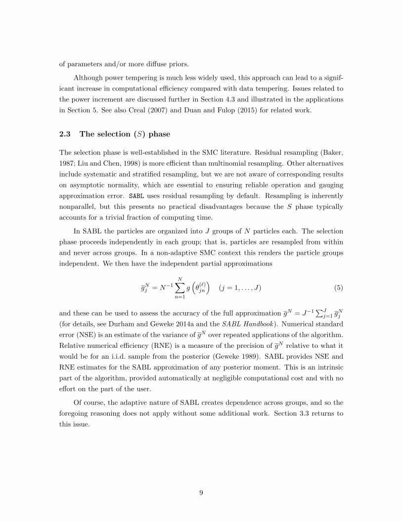
In SABL the particles are organized into J groups of N particles each. The selection

phase proceeds independently in each group; that is, particles are resampled from within

and never across groups. In a non-adaptive SMC context this renders the particle groups

independent. We then have the independent partial approximations

gNj = N−1N∑n=1

g(θ

(`)jn

)(j = 1, . . . , J) (5)

and these can be used to assess the accuracy of the full approximation gN = J−1∑J

j=1 gNj

(for details, see Durham and Geweke 2014a and the SABL Handbook). Numerical standard

error (NSE) is an estimate of the variance of gN over repeated applications of the algorithm.

Relative numerical efficiency (RNE) is a measure of the precision of gN relative to what it

would be for an i.i.d. sample from the posterior (Geweke 1989). SABL provides NSE and

RNE estimates for the SABL approximation of any posterior moment. This is an intrinsic

part of the algorithm, provided automatically at negligible computational cost and with no

effort on the part of the user.

Of course, the adaptive nature of SABL creates dependence across groups, and so the

foregoing reasoning does not apply without some additional work. Section 3.3 returns to

this issue.

9

2.4 The mutation (M) phase

At the conclusion of the S phase the particles are dependent: some are repeated while others

have been eliminated. If the algorithm had no mutation (move) phase then the number of

distinct particles would be weakly monotonically decreasing from one cycle to the next. In

the application of SMC to Bayesian inference it is easy to verify that for any given number

of particles and under mild regularity conditions for the likelihood function the number of

distinct particles would diminish to one and RNE would go to zero as sample size increases.

The idea of incorporating one or more Metropolis steps to rejuvenate the sample of particles

(thus improving RNE) goes back to at least Gilks and Berzuini (2001).

The M phase is standard MCMC, but operating on the entire sample {θjn} in parallel

rather than on a single parameter vector sequentially. This is the key to the computational

efficiency of the SABL algorithm, since it implies that the algorithm is inherently amenable

to implementation using inexpensive and powerful parallel computing hardware. The other

key element that makes this method attractive relative to conventional MCMC is that the

full sample of particles is available for use in constructing proposal densities, avoiding the

need for tedious tuning and experimentation. The entire process is automated, requiring

no judgemental inputs on the part of the user.

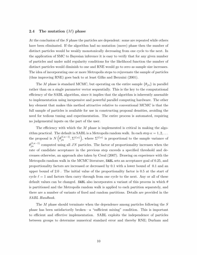
The efficiency with which the M phase is implemented is critical in making the algo-

rithm practical. The default in SABL is a Metropolis random walk. In each step κ = 1, 2, . . .

the proposal is N(θ

(`,κ−1)jn ,Σ(`,κ)

), where Σ(`,κ) is proportional to the sample variance of

θ(`,κ−1)jn computed using all JN particles. The factor of proportionality increases when the

rate of candidate acceptance in the previous step exceeds a specified threshold and de-

creases otherwise, an approach also taken by Creal (2007). Drawing on experience with the

Metropolis random walk in the MCMC literature, SABL sets an acceptance goal of 0.25, and

proportionality factors are increased or decreased by 0.1 with a lower bound of 0.1 and an

upper bound of 2.0 . The initial value of the proportionality factor is 0.5 at the start of

cycle ` = 1 and factors then carry through from one cycle to the next. Any or all of these

default values can be changed. SABL also incorporates a variant of this process in which θ

is partitioned and the Metropolis random walk is applied to each partition separately, and

there are a number of variants of fixed and random partitions. Details are provided in the

SABL Handbook.

The M phase should terminate when the dependence among particles following the S

phase has been satisfactorily broken—a “sufficient mixing” condition. This is important

to efficient and effective implementation. SABL exploits the independence of particles

between groups to determine numerical standard error and thereby RNE; Durham and

10

Geweke (2014a, Section 2.3) provides details. SABL is therefore able to track the RNE

of some simple, model-specific functions of the particles at each step κ of the Metropolis

random walk. Typically RNE increases, with some noise, as the steps proceed. The M

phase and the cycle terminate when the average RNE across the tracking functions reaches

a specified target. SABL uses one target (default value 0.4) for all cycles except the last,

which has its own target (default value 0.9). Default values can again be made model or

application specific. See Durham and Geweke (2014a) for additional details.

3 Foundations of the SABL algorithm

Like all posterior simulators, including importance sampling and Markov chain Monte Carlo,

SMC algorithms represent a posterior distribution by means of a collection of parameter

vectors (particles) simulated from an approximating distribution. Posterior moments are

approximated by computing (weighted) sample averages over these simulated parameter

draws. The underlying theory, like that for importance sampling and MCMC, must carefully

characterize the approximation error and the ways in which it can be made arbitrarily

small. The focus is on conditions under which the simulated draws are ergodic and the

approximation error has a limiting normal distribution.

To develop this theoretical foundation for the SABL algorithm, first consider non-

adaptive SMC algorithms in which there is no feedback from the simulated particles to

the design of the algorithm: specifically, the kernels k(`) are fixed at the outset rather

than being determined on-the-fly in the C phase; and the proposal densities for Metropolis

steps in the M phase as well as the number of Metroplis iterations in each cycle are also

fixed at the outset. Douc and Moulines (2008) provide careful consistency and asymptotic

normality results for such non-adaptive SMC algorithms. Section 3.1 restates their results

in the context of the Bayesian inference problem taken up here.

Verifying sufficient conditions for consistency and asymptotic normality is essential to

careful application of any SMC algorithm, including SABL. A similar requirement pertains

to any posterior simulator. Section 3.2 takes up the most important aspects of this process.

The conditions as actually stated by Douc and Moulines (2008) are of a recursive nature

such that direct verification is essentially impossible, and we are aware of no applied work

using algorithms similar to SABL in which verification of the conditions is demonstrated.

We restate these conditions in a form that greatly simplifies verification and show that these

conditions are in fact closely related to well-known conditions for importance sampling. We

also show that there are important cases where verification is simpler when power tempering

rather than data tempering is used.

11

While the results of Douc and Moulines (2008) are sufficient for non-adaptive SMC,

there are no comparable results for the kinds of adaptive algorithms used in practice.

Durham and Geweke (2014a) proposes a two-pass procedure that allows for algorithms

making use of the adaptive learning that is essential for practical application while still

satisfying the conditions underlying Douc and Moulines (2008). Section 3.3 recapitulates

this procedure, extending the theory to adaptive SMC algorithms in general and to SABL

in particular.

3.1 Formal conditions

All desirable properties of SMC algorithms, including SABL, are asymptotic in the number

of particles N . SABL maintains J groups of particles to facilitate the construction of

numerical standard errors of approximation, but this is incidental to convergence in N . The

formal development of the theory treats the limiting distribution (in N) of the triangular

array {θ N,i} (i = 1, . . . , N ;N = 1, 2, . . .), and this section uses that notation.

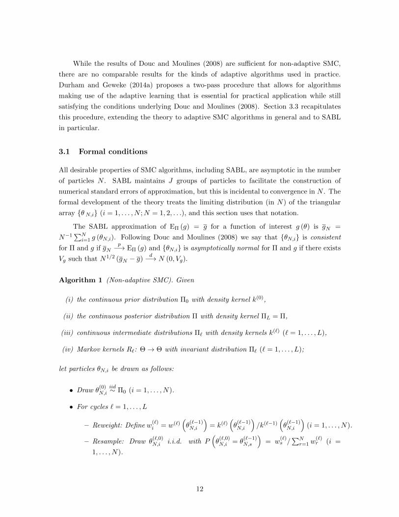
The SABL approximation of EΠ (g) = g for a function of interest g (θ) is gN =

N−1∑N

i=1 g (θN,i). Following Douc and Moulines (2008) we say that {θN,i} is consistent

for Π and g if gNp−→ EΠ (g) and {θN,i} is asymptotically normal for Π and g if there exists

Vg such that N1/2 (gN − g)d−→ N (0, Vg).

Algorithm 1 (Non-adaptive SMC). Given

(i) the continuous prior distribution Π0 with density kernel k(0),

(ii) the continuous posterior distribution Π with density kernel ΠL = Π,

(iii) continuous intermediate distributions Π` with density kernels k(`) (` = 1, . . . , L),

(iv) Markov kernels R`: Θ→ Θ with invariant distribution Π` (` = 1, . . . , L);

let particles θN,i be drawn as follows:

• Draw θ(0)N,i

iid∼ Π0 (i = 1, . . . , N).

• For cycles ` = 1, . . . , L

– Reweight: Define w(`)i = w(`)

(θ

(`−1)N,i

)= k(`)

(θ

(`−1)N,i

)/k(`−1)

(θ

(`−1)N,i

)(i = 1, . . . , N).

– Resample: Draw θ(`,0)N,i i.i.d. with P

(θ

(`,0)N,i = θ

(`−1)N,s

)= w

(`)s /

∑Nr=1w

(`)r (i =

1, . . . , N).

12

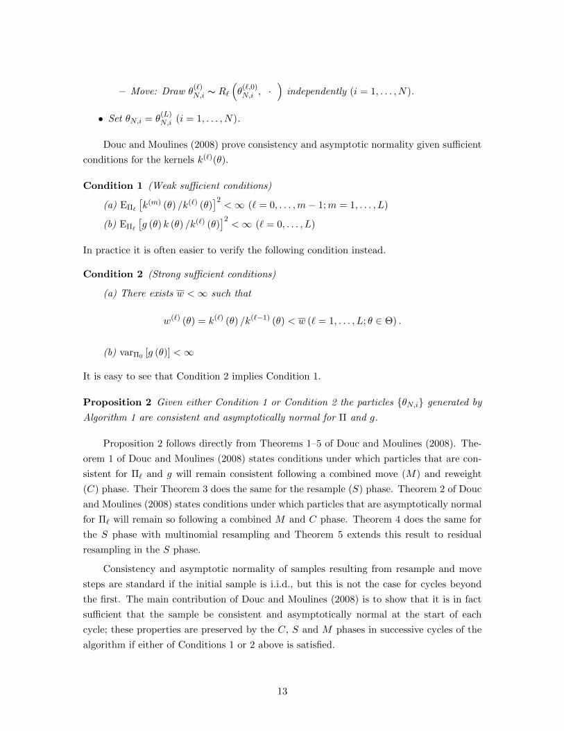
– Move: Draw θ(`)N,i ∼ R`

(θ

(`,0)N,i , ·

)independently (i = 1, . . . , N).

• Set θN,i = θ(L)N,i (i = 1, . . . , N).

Douc and Moulines (2008) prove consistency and asymptotic normality given sufficient

conditions for the kernels k(`)(θ).

Condition 1 (Weak sufficient conditions)

(a) EΠ`

[k(m) (θ) /k(`) (θ)

]2<∞ (` = 0, . . . ,m− 1;m = 1, . . . , L)

(b) EΠ`

[g (θ) k (θ) /k(`) (θ)

]2<∞ (` = 0, . . . , L)

In practice it is often easier to verify the following condition instead.

Condition 2 (Strong sufficient conditions)

(a) There exists w <∞ such that

w(`) (θ) = k(`) (θ) /k(`−1) (θ) < w (` = 1, . . . , L; θ ∈ Θ) .

(b) varΠ0 [g (θ)] <∞

It is easy to see that Condition 2 implies Condition 1.

Proposition 2 Given either Condition 1 or Condition 2 the particles {θN,i} generated by

Algorithm 1 are consistent and asymptotically normal for Π and g.

Proposition 2 follows directly from Theorems 1–5 of Douc and Moulines (2008). The-

orem 1 of Douc and Moulines (2008) states conditions under which particles that are con-

sistent for Π` and g will remain consistent following a combined move (M) and reweight

(C) phase. Their Theorem 3 does the same for the resample (S) phase. Theorem 2 of Douc

and Moulines (2008) states conditions under which particles that are asymptotically normal

for Π` will remain so following a combined M and C phase. Theorem 4 does the same for

the S phase with multinomial resampling and Theorem 5 extends this result to residual

resampling in the S phase.

Consistency and asymptotic normality of samples resulting from resample and move

steps are standard if the initial sample is i.i.d., but this is not the case for cycles beyond

the first. The main contribution of Douc and Moulines (2008) is to show that it is in fact

sufficient that the sample be consistent and asymptotically normal at the start of each

cycle; these properties are preserved by the C, S and M phases in successive cycles of the

algorithm if either of Conditions 1 or 2 above is satisfied.

13

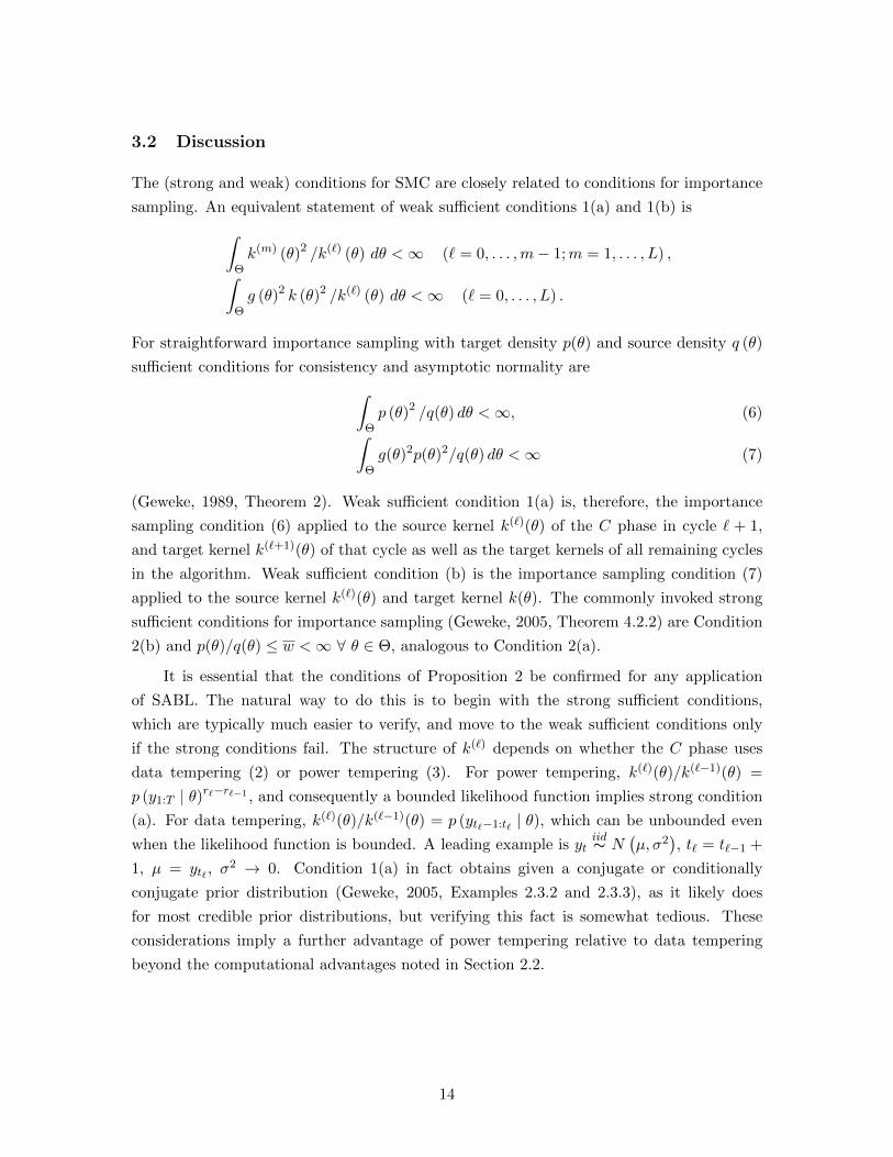
3.2 Discussion

The (strong and weak) conditions for SMC are closely related to conditions for importance

sampling. An equivalent statement of weak sufficient conditions 1(a) and 1(b) is∫Θk(m) (θ)2 /k(`) (θ) dθ <∞ (` = 0, . . . ,m− 1;m = 1, . . . , L) ,∫

Θg (θ)2 k (θ)2 /k(`) (θ) dθ <∞ (` = 0, . . . , L) .

For straightforward importance sampling with target density p(θ) and source density q (θ)

sufficient conditions for consistency and asymptotic normality are∫Θp (θ)2 /q(θ) dθ <∞, (6)∫

Θg(θ)2p(θ)2/q(θ) dθ <∞ (7)

(Geweke, 1989, Theorem 2). Weak sufficient condition 1(a) is, therefore, the importance

sampling condition (6) applied to the source kernel k(`)(θ) of the C phase in cycle ` + 1,

and target kernel k(`+1)(θ) of that cycle as well as the target kernels of all remaining cycles

in the algorithm. Weak sufficient condition (b) is the importance sampling condition (7)

applied to the source kernel k(`)(θ) and target kernel k(θ). The commonly invoked strong

sufficient conditions for importance sampling (Geweke, 2005, Theorem 4.2.2) are Condition

2(b) and p(θ)/q(θ) ≤ w <∞ ∀ θ ∈ Θ, analogous to Condition 2(a).

It is essential that the conditions of Proposition 2 be confirmed for any application

of SABL. The natural way to do this is to begin with the strong sufficient conditions,

which are typically much easier to verify, and move to the weak sufficient conditions only

if the strong conditions fail. The structure of k(`) depends on whether the C phase uses

data tempering (2) or power tempering (3). For power tempering, k(`)(θ)/k(`−1)(θ) =

p (y1:T | θ)r`−r`−1 , and consequently a bounded likelihood function implies strong condition

(a). For data tempering, k(`)(θ)/k(`−1)(θ) = p (yt`−1:t` | θ), which can be unbounded even

when the likelihood function is bounded. A leading example is ytiid∼ N

(µ, σ2

), t` = t`−1 +

1, µ = yt` , σ2 → 0. Condition 1(a) in fact obtains given a conjugate or conditionally

conjugate prior distribution (Geweke, 2005, Examples 2.3.2 and 2.3.3), as it likely does

for most credible prior distributions, but verifying this fact is somewhat tedious. These

considerations imply a further advantage of power tempering relative to data tempering

beyond the computational advantages noted in Section 2.2.

14

3.3 The two-pass algorithm

As described in Section 2 the SABL algorithm determines the kernels k(`) in the C phase of

successive cycles using information in the JN particles θ(`−1)jn and determines the proposal

density and number of iterations for the Metropolis random walk in the M phase using

information in the succession of particles θ(`,κ−1)jn (κ = 1, 2, . . .). These critical adaptations

are precluded by existing SMC theory, including Proposition 2. Indeed, essentially any

practical implementation of SMC for posterior simulation must include adaptation to be

useful and is therefore subject to this issue.

SABL resolves this problem and achieves analytical integrity by utilizing two passes.

The first pass is the adaptive variant in which the algorithm is self-modifying. The second

pass fixes the design emerging from the first pass and then executes the fixed Bayesian

learning algorithm to which Proposition 2 applies. (Durham and Geweke 2014a and the

SABL Handbook provide further details.) This feature is fully implemented in the SABL

software package and requires minimal effort on the part of the user.

4 The SABL algorithm for optimization

The sequential Monte Carlo (SMC) literature has recognized that those algorithms can be

applied to optimization problems by concentrating the distribution of particles from what

otherwise would be the likelihood function more and more tightly about its mode (Del

Moral et al. 2006; Zhou and Chen 2013). Indeed, if the objective function is the likelihood

function itself, the result would be a distribution of particles near the likelihood function

mode, converging to the maximum likelihood estimator. The basic idea is straightforward:

apply power tempering in the C phase but continue with cycles increasing the power r` well

beyond the value r` = 1 that defines the likelihood function itself. The principle is sound

but, as is so often the case, developing details that are simultaneously careful, precise and

practical is the greater challenge. To the best of our knowledge these details have not been

developed in the literature. This section discusses some of the key issues involved and the

result is incorporated in the SABL software package.

4.1 The optimization problem

This section adopts notation and terminology from the global optimization literature, and

specifically the simulated annealing literature to which SABL is most closely related and

upon which SABL provides substantial improvement. The objective function is h(θ) : Θ→

15

R and the associated Boltzman kernel for the optimization problem is

k (θ;h, p0, r) = p0(θ) exp [r · h(θ)] , (8)

which is the analog of the target kernel k(θ) from Section 2. The initial density p0(θ) is a

technical device required for SABL as it is for simulated annealing. In the optimization liter-

ature p0(θ) is sometimes called the instrumental distribution. When used for optimization,

the final result of the algorithm does not depend on p0 (whereas when used for Bayesian

inference the posterior distribution clearly depends on the prior distribution). The argu-

ments h and p0 will generally be suppressed in the sequel unless needed to avoid ambiguity.

Let µ denote Borel measure.

Let h = supΘ h(θ). Fundamental both to the theory and practice is the upper contour

set Θ(ε, h) defined for all ε > 0 as

Θ(ε;h) =

{θ : h(θ) > h− ε

}if h <∞

{θ : h(θ) > 1/ε} if h =∞.

Also define the modal set Θ = limε→0 Θ (ε;h).

The following basic conditions are needed.

Condition 3 (Basic conditions.)

(a) µ [Θ (ε;h)] > 0 ∀ ε > 0;

(b) 0 < p = infθ∈Θ p0(θ) ≤ supθ∈Θ p0(θ) = p <∞;

(c) For all r ∈ [0,∞),∫

Θ k(θ; r) dθ <∞.

Condition 3 is easily violated when the optimization problem is maximum likelihood.

A classic example is maximum likelihood estimation in a full mixture of normals model

(the likelihood function is unbounded when one component of the mean is exactly equal to

one of the data points and the variance of that component approaches zero). This is not

merely an academic nicety, because when SABL is applied to optimization problems it really

does isolate multiple modes and modes that are unbounded. These problems are avoided in

some approaches to optimization, including implementations of the EM algorithm, precisely

because those approaches fail to find the true mode in such cases. More generally, this

section carefully develops these and other conditions because they are essential to fully

understanding what happens when SABL successfully maximizes objective functions that

violate standard textbook assumptions but arise routinely in economics and econometrics.

16

A few more definitions are required before stating the basic result and proceeding

further. These definitions presume Condition 3. Associated with the objective function

h(θ), the associated Boltzman kernel (8), and the initial density p0, the Boltzman density is

p(θ;h, p0, r) = k(θ;h, p0, r)/∫

Θ k(θ;h, p0, r) dθ; the Boltzman probability is P (S;h, p0, r) =∫S k(θ;h, p0, r) dθ for all Borel sets S ⊆ Θ; and the Boltzman random variable is θ(h, p0, r)

with P(θ(h, p0, r) ∈ S

)= P (S;h, p0, r) for all Borel sets S ⊆ Θ. Again, the arguments h

and p0 will generally be suppressed unless needed to avoid ambiguity.

The result of primary interest is the following.

Proposition 3 (Limiting particle concentration.) Given Condition 3,

limr→∞

P [Θ (ε;h) ; r] = 1 ∀ ε > 0.

Proof. See Section 7.

In interpreting the results of the SABL algorithm in situations that differ from the

“standard” problem of a bounded continuous objective function with a unique global mode

discretely greater than the value of h(θ) at the most competitive local mode, it is important

to bear in mind Proposition 3. It states precisely the regions of Θ in which particles

will be concentrated as r → ∞; the relationship of these subsets to the global mode(s)

themselves is a separate matter and many possibilities are left open under Condition 3.

This is intentional. SABL succeeds in these situations when other approaches can fail, but

the definition of success—which is Proposition 3—is critical.

4.2 Global convergence

This section turns to conditions under which SABL provides a sequence of particles con-

verging to the true mode.

Condition 4 (Singleton global mode.)

(a) The modal set{

Θ = θ∗}

, is a single point.

(b) For all δ > 0 there exists ε > 0 such that

Θ(ε;h) ⊆ B(θ∗; δ)def={θ : (θ − θ∗)′(θ − θ∗) < δ2

}.

Proposition 4 (Consistency of mode determination.) Given Conditions 3 and 4,

limr→∞

P [B (θ∗; δ) ; r] = 1 ∀ δ > 0.

17

Proof. Immediate from Proposition 3.

Given Condition 4(a) it is still possible that the competitors to θ∗ belong to a set

remote from θ∗. A simple example is Θ = (0, 1), h (1/2) = 1, h(θ) = 2 |θ − 0.5| ∀ θ ∈(0, 1/2) ∪ (1/2, 1). Condition 4(b) makes this impossible.

Condition 4(a) is not necessary for SABL to provide constructive information about

Θ. Indeed when Θ is not a singleton the algorithm performs smoothly whereas it can be

difficult to learn about Θ using some alternative optimization methods.

For example, consider the family of functions h(θ) = (θ − θ∗)′A (θ − θ∗), where Θ =

Rm (m > 1) and A is a negative semidefinite matrix of rank l < m. Then Θ is an entire

Euclidean space of dimension m− l. Particle variation orthogonal to this space vanishes as

r →∞, but the distribution of particles within this space depends on p0(θ).

The following regularity conditions are familiar from econometrics.

Condition 5 (Mode properties.)

(a) The initial density p0(θ) is continuous at θ = θ∗;

(b) There is an open set S such that θ∗ ∈ S ⊆ Θ;

(c) At all θ ∈ Θ, h(θ) is three times differentiable and the third derivatives are uniformly

bounded on Θ;

(d) At θ = θ∗, ∂h(θ)/∂θ = 0, H = ∂2h(θ)/∂θ∂θ′ is negative definite, and the third

derivatives of h(θ) are continuous.

In the econometrics context the following result is perhaps unsurprising, but it has

substantial practical value.

Proposition 5 (Asymptotic normality of particles.) Given Conditions 3, 4 and 5, as r →∞, u (r) = r1/2

[θ(r)− θ∗

]d−→ N

(0,−H−1

).

Proof. See Section 7.

Denote the population variance of the particles at power r by Vr. Proposition 5 shows

that given Conditions 4 and 5 limr→∞ rVr = −H−1. Let Vr,N denote the corresponding

sample variance of particles. By ergodicity of the algorithm limN→∞ limr→∞ rVr,N = −H−1.

The result has significant practical implications for maximum likelihood estimation, because

it provides the asymptotic variance of the estimator as a costless by-product of the SABL

algorithm. Condition 5 has much in common with the classical conditions for the asymptotic

variance of the maximum likelihood estimator due to the similarity of the derivations, but

18

the results do not. Whereas the classical conditions are sufficient for the properties of

the variance of the maximum likelihood estimator in the limit as sample size increases,

Conditions 4 and 5 are sufficient for limN→∞ limr→∞ rVr,N = −H−1 regardless of sample

size.

The following modest extension of Proposition 5 is often useful, as illustrated subse-

quently in Section 5.2.2.

Condition 6 g : Θ → Γ ⊆ Rm is continuous with continuous first and second derivatives

on the set S of Condition 5.

Corollary 1 Given Conditions 3–6,

r1/2

(g(θ (r)

)− g∗

θ (r)− θ∗

)d−→ N

(0,−

[g∗1H

−1g∗′1 g∗1H−1

H−1g∗′1 H−1

])

where

g∗ = g (θ∗) , g∗1 = ∂g (θ∗) /∂θ′.

Proof. Follows immediately as an elementary asymptotic expansion (Cramer, 1946, Section

28.4).

Denote the population covariance of the particles θ(`)N,i with the values g(θ

(`)N,i) at power

r = r` by cr. Corollary 1 shows that limr→∞ r ·V −1r ·cr = g∗′1 . Consequently in an estimated

linear regression of g(θ(`)N,i) on an intercept and θ

(`)N,i (i = 1, . . . , N) the coefficients on the

components of θ converge to g∗1 as r →∞, N →∞. (Note that while the theory here and

in Section 3 is developed for a single block of N particles, in practice SABL evaluates this

regression across all JN particles; it is easy to see that the result extends to this context.)

4.3 Rates of convergence

One can also determine the limiting (as `→∞) properties of the power tempering sequence

{r`}. This requires no further conditions. The result shows that the growth rate of power

ρ` = (r` − r`−1)/r`−1 converges to a limit that depends on the dimension of Θ but is

otherwise independent of the optimization problem. Suppose that Θ ⊆ Rm.

Proposition 6 (Rate of convergence.) Given Conditions 4 and 5, the limiting value of the

growth rate of power ρ` for the power tempering sequence defined by (4) and the equation

19

f(r`) = RESS∗ is

ρ = lim`→∞

ρ` = (RESS∗)−2/m − 1 +{[

(RESS∗)−2/m − 1]

(RESS∗)−2/m}1/2

. (9)

Proof. See Section 7.

Suppose that in Proposition 6, RESS∗ = 0.5, which is the default value in SABL. If

the objective function has m = 2 parameters then ρ = 2.412; for m = 5, ρ = 0.968; for

m = 20, ρ = 0.3491; and for m = 100, ρ = 0.1329. The SABL algorithm regularly produces

sequences ρ` very close to the limiting value identified in Proposition 6 over successive

cycles as illustrated subsequently in Section 5. These rates of increase are quite high by

the standards of the simulated annealing literature (e.g. Zhou and Chen 2013) and as a

consequence SABL approximates global modes to a given standard of approximation much

faster.

A straightforward reading of Proposition 6 suggests that in the limit, each incremental

cycle leads to a predictable growth rate of power with an attendant increase in the concen-

tration of particles around θ∗. However, this does not persist indefinitely. The limitations of

machine precision make it impossible to distinguish between values of the objective function

h whose ratio is of the order of 1+ε, or less, where ε = 2−b and b is the number of mantissa

bits in floating point representation. In a standard 64-bit environment ε ≈ 2.22 × 10−16.

As this point is approached the computed values h(θ

(`)N,i

)(i = 1, 2, . . . , N) take on only

a few discrete values and their distribution looks less and less like a normal distribution.

The Gaussian proposals in the random walk Metropolis steps of the M phase become cor-

respondingly ill-suited and the growth rate of power, ρ`, declines toward zero. This results

in time-consuming cycles that provide almost no improvement in the approximation of θ∗.

As a practical matter it is therefore important to have a stopping criterion that avoids

these useless iterations. Fortunately there is a robust and practical treatment of this prob-

lem, which emerged from our experience with quite a few optimization problems. The key

to the approach lies in Proposition 5. So long as the distribution of h(θ) across the particles

continues to be dominated by the normal asymptotics, the values h (θ) are increasingly well-

approximated by a quadratic function of θ. As finite precision arithmetic becomes more

important, the quality of this approximation decreases. As a consequence, the conventional

R2 from a linear regression of h(θ

(`)N,i

)on the particles θ

(`)N,i and quadratic interaction terms

is a reliable indicator: so long as R2 increases over successive cycles the normal asymptotics

dominate, but as R2 decreases the investment in additional cycles yields little information

about θ∗. Examples in Section 5 exhibit R2 > 0.99 for long sequences of cycles.

20

Our experience is that monitoring this R2 is more reliable than monitoring the rate

of power increase ρ`, although, as examples in Section 5 illustrate, their trajectories are

mutually consistent. Our current practice, reflected in the optimization examples of Section

5, is to halt the algorithm at cycle ` if the maximum value of R2 occurred at cycle `− 10.

Then, use the particle distribution in cycle ` − 10 to approximate θ∗. By experimenting

with problems in which the exact θ∗ is known, we have concluded that the most reliable

approximation of θ∗ is the mean of the particles. In particular, results are more satisfactory

when considering all of the particles as opposed to (say) only those particles that correspond

to the largest computed value h (θ). The reason is that differences among the largest values

of h (θ) are most sensitive to the effects of finite precision arithmetic. The mean of the

particles, on the other hand, exploits the quadratic approximation and in so doing reduces

the influence of finite precision arithmetic.

5 Examples

Applications of SABL or similar approaches in economics and finance include Creal (2012),

Fulop (2012), Durham and Geweke (2014a), Herbst and Schorfheide (2014), Blevins (2016)

and Geweke (2016). This section takes up examples that appear in none of these papers

but have been used as case studies for other posterior simulation methods (Ardia et al.

2009, 2012; Hoogerheide et al. 2012; Basturk et al. 2016, 2017). The intention is to

clearly illustrate the main points of Sections 2 through 4 and facilitate comparison with the

performance of alternatives to SABL.

5.1 A family of bivariate distributions

Gelman and Meng (1991) noted that in the bivariate distribution with kernel

f (θ1, θ2) = exp

[−1

2

(Aθ2

1θ22 + θ2

1 + θ22 − 2Bθ1θ2 − 2C1θ1 − 2C2θ2

)](10)

(A > 0, or A = 0 and |B| < 1), both conditional densities are Gaussian but the joint

distribution is not. The distribution is a popular choice for applications and case studies

in the Monte Carlo integration literature (Kong et al. 2003; Ardia et al. 2009). Basturk et

al. (2016, 2017) importance sample from this distribution using a source distribution that

is an adaptive mixture of Student-t distributions.

The density kernel (10) can be expressed as the product of a bivariate Gaussian kernel

and a remainder, which can then be taken as the “prior” kernel and “likelihood”, respec-

21

tively, in the SABL algorithm. To this end define B∗ = min (1− ε, max (ε− 1, B)), so that

|B∗| < 1− ε for some small ε > 0. The respective kernels are

k0 (θ1, θ2) = (2π)−1 |V |−1/2 exp

[−1

2(θ − µ)′ V −1 (θ − µ)

],

where

V =(1−B∗2

)−1

[1 B∗

B∗ 1

], µ = V

(C1

C2

),

and

k∗ (θ1, θ2) = 2π |V | exp

{−1

2

[Aθ2

1θ22 − (B −B∗) θ1θ2 − µ′µ

]}.

Basturk et al. (2016, 2017) illustrate their adaptive importance sampling approach for

the Cases A = 1, B = 0, C1 = C2 = 3 (Case 1) and A = 1, B = 0, C1 = C2 = 6

(Case 2). We consider these and two others: A = 1, B = 0, C1 = C2 = 9 (Case 3) and

A = 1, B = 4, C1 = C2 = 80 (Case 4). Figure 1 shows scatterplots of the particles at

the conclusion of the SABL algorithm for Cases 1–4, respectively. The four iso-contours,

computed directly from (10), are selected to include 98%, 75%, 50% and 25% of the particles

in their interiors, respectively. The comparison shows that the particles are faithful to the

shape of the Gelman-Meng distribution.

Table 1 provides information about the performance of the SABL algorithm.2 All four

cases used the default SABL settings for the algorithm. In particular, there were 214 =

16, 384 particles. For this example, equivalent results can be obtained with 212 = 4, 096

particles, which reduces computing time and function evaluations by a factor of about 4

while the other entries in Table 1 are similar. The variation in the performance of the

algorithm among the four cases can be traced to the varying suitability of the random

walk Metropolis step in the M phase. Recall from Section 2 that the variance of the

proposal density is proportional to the sample variance of the particles. In Case 1 the global

correlation between θ1 and θ2 is similar to the local correlation of particles around each

mode, but in the other cases the global correlation of particles is less helpful in constructing

productive Metropolis steps and so M phase sampling is less efficient. The issue is most

severe in Case 3.

Basturk et al. (2017) provide enough information about the performance of the adaptive

importance sampling for Case 1 to permit comparison of the efficiency of that approach with

SABL. The RNE of the two approaches is about the same. Basturk et al. (2017) report

computation time of about 17 seconds to generate a Monte Carlo sample of size 10,000. The

2All calculations for Section 5 were carried out on a MacBook Pro (Retina, Mid 2012), 2.6 GHz Intelquadcore i7 processor, 16GB memory using Matlab 2016b incorporating the SABL toolbox.

22

straightforward implication of Table 1 is that SABL is about 17 times faster, but this does

not account for differences in computing environment, and Basturk et al. do not report the

number of function evaluations. More important, perhaps, the SABL algorithm achieves

this using default settings with no tinkering required by the user. Multimodality, even in

the somewhat pathological Case 3, is handled effortlessly.

5.2 GARCH with Student-t innovations

The GARCH(1,1) model with Student-t innovations is a reasonably good representation of

returns for many financial assets and has become a staple of applied financial econometrics

(Hansen and Lunde, 2005; Zivot, 2009). The likelihood function is unimodal but sufficiently

non-elliptical that it can pose practical problems for conventional inference based on max-

imum likelihood (Zivot, 2009). The model has been a testbed for alternative Monte Carlo

approximations of posterior moments (Ardia et al., 2012; Hoogerheide et al., 2012; Basturk

et al., 2017).

We use standard notation for the model,

yt = µ+ h1/2t εt; ht = ω + α (yt−1 − µ)2 + βht−1; εt

iid∼ t (ν) ,

where yt is the observed return, ht is the variance of yt conditional on its past and t(ν) is

the Student-t distribution with ν degrees of freedom. Following Basturk et al. (2016) h0 is

fixed to the sample variance of yt. The data are S&P 500 daily log returns from January

3,1990 through October 9, 2015, a total of 6493 observations.

As usual, the only effort required on the part of the user for both Bayesian inference and

optimization is code evaluating the likelihood of yt|y1:t−1. Estimates of numerical standard

error are provided as a standard output at no cost, either computationally or in user effort.

5.2.1 Bayesian inference

Following Basturk et al. (2016) the prior distributions are independent and uniform, on

[−1, 1] for µ, (0, 1] for ω, the unit simplex for (α, β), and (2, 20] for ν. Sampling from the

posterior distribution is a straightforward task in SABL, using either power tempering or

data tempering. Table 2 compares the computational performance of the two approaches. In

the table a component evaluation is an evaluation of the contribution of one observation to

the log-likelihood function evaluated at one particle. Data tempering, proceeding through

thousands of observations, requires more cycles and M phase iterations; but it entails

fewer component evaluations because most of the cycles involve relatively few observations

23

(e.g. at cycle 60 only the first 1856 observations have been introduced via the C phase). As

a consequence data tempering requires about 10% less time than power tempering.

More important than computation time, Bayesian inference in the GARCH model

proceeds smoothly using the default settings in the SABL software. The final target average

RNE of 0.9, for the five parameters, is reflected in the entries for RNE in Table 3. The

results show that the particles are close to independent, making for an efficient Monte Carlo

sample from the posterior distribution.

Summary statistics and pairwise scatterplots of the sampled particles are shown in

Table 3 and Figure 2, respectively. The posterior density is apparently unimodal and

concave in all relevant highest density confidence regions. The distributions of individual

parameters are close to Gaussian (Table 3). Pairs of parameters exhibit the same weak

departure from an elliptical distribution (Figure 2). All pairs of parameters except (α, β)

are weakly correlated.

5.2.2 Maximum likelihood

As described in Section 4 the SABL power tempering algorithm for Bayesian inference

converges to maximum likelihood point estimates simply by allowing the power to increase.

No further investment in code is required. This is especially attractive when analytical first

and second derivatives are unavailable and tedious to derive. In the case of GARCH, they

are known (Fiorentini et al., 1996), but this model provides a convenient venue to illustrate

the convergence properties of the SABL optimization algorithm discussed in Section 4.

Parameter estimates and standard errors are shown in Table 4. Implied classical bivari-

ate asymptotic distributions are represented by the ellipses in Figure 2. Posterior means

and maximum likelihood estimates are close, relative to the relevant posterior marginal

distributions, as indicated in this figure and by comparison of the results in Tables 3 and 4.

Figure 3 monitors the power and the distribution of particles, by cycle, with reference

to Propositions 5 and 6. In the middle panel, distance from quadratic is 1 − R2 in the re-

gression of the log likelihood on an intercept, each element of the particle vector, and their

squares and cross-products. The asymptotics of optimization are reflected clearly in cycles

21 through 28, in which the log likelihood is very close to quadratic (middle panel) and

increments to power are close to the asymptotic rate ρ indicated by the dashed line (lower

panel). In earlier cycles the asymptotic normality has not yet emerged; later cycles exhibit

non-normality as the powered log-likelihood function moves toward a step function (as dic-

tated by finite-precision arithmetic when the distribution of particles becomes increasingly

concentrated near the mode). The log-likelihood is closest to a quadratic function of the

24

parameters at cycle 25 (R2 = 0.9986 in the regression discussed in Section 4).

While the GARCH(1,1) model is widely used, it fails to account for important features

of asset returns. For example, leverage effects are omitted; and although the model captures

much of the heteroskedasticity of returns, models with two volatility factors are preferred

(Durham and Geweke 2014b) . In such circumstances the Hessian is not consistent for the

asymptotic variance of the MLE and the Huber “sandwich” variance estimate is preferred,

[∂2` (θ)

∂θ∂θ′

]−1

·

[T∑t=1

∂`t (θ)

∂θ· ∂`t (θ)

∂θ′

]·[∂2` (θ)

∂θ∂θ′

]−1

, (11)

where ` (θ) =∑T

t=1 `t (θ) is the log-likelihood function and all derivatives in (11) are

evaluated at the maximum likelihood estimate θ = θ. The derivatives ∂`t(θ)/∂θ′ and

∂2`(θ)/(∂θ∂θ′) are easily approximated using coefficients from the regressions of `t(θjn)

(t = 1, 2, . . . , T ) and `(θjn) on linear and quadratic functions, respectively, of the JN parti-

cles θjn at the chosen cycle (cycle 25, which minimizes departure of the log-likelihood from

a quadratic function, in this example). Computational cost and effort required on the part

of the user are both minimal.

The last row of Table 4 provides the implied robust standard errors at cycle 25. The

contrast between classical and robust standard errors is striking: sandwich standard errors

for the mean µ are on the order of one-tenth the classical standard errors, whereas for ω

they are nearly double.

5.3 Instrumental variables

This section looks at the performance of SABL in the simplest possible linear simultaneous

equations setting: a single, exactly identified equation; equivalently, a linear model with a

single (endogenous) covariate and a single instrument. This is a much-examined setting in

econometrics, including Bayesian inference (Dreze 1976, 1977; Geweke 1996; Kelibergen and

Van Dijk 1998; Hoogerheide et al. 2007). Our examples all employ proper prior distribu-

tions for the structural parameters, avoiding the pitfall of improper posterior distributions.

The proper priors are quite diffuse, in order to highlight the contribution of the likelihood

function and provide comparability with a long literature on recovering posterior distribu-

tions in this situation (in addition to the references just cited, on this point see Zellner et

al. 2014 and Basturk et al. 2016, 2017).

There are three examples in this section. The first one (Section 5.3.1) is the same pub-

lished example studied in Basturk et al. (2016). The other two examples use artificial data

to set up situations with very poor instruments. In the first (Section 5.3.2) the structural

25

equation parameters are unidentified in the population, but the sample correlation between

instrument and covariate is not zero. In the second (Section 5.3.3) this sample correlation

coefficient is exactly zero.

These examples take up both the representation of the posterior distribution and the

computation of maximum likelihood estimates using SABL. Bayesian inference using SABL

is entirely routine. Using the SABL software with all default settings, representations of the

posterior distribution are computed in a matter of a few seconds on a conventional laptop

in all cases. The computations appear to be about 100 times faster than those reported by

Basturk et al. (2016, 2017), which in turn outperform conventional approaches like Markov

chain Monte Carlo. Maximum likelihood estimation is also routine and recovers the exact

asymptotic distributions up to numerical standard error, which in turn is small.

5.3.1 Comparative development example

Acemoglu et al. (2001) studied the relationship between endogenous variables log GDP per

capita in 1995 (yi) and average protection against expropriation risk in 1985-1995 (xi) in

the linear model yi = α1 +α2xi + εi. The instrument (zi) is log European settler mortality.

The model isyi = α1 + α2xi + εi

xi = β1 + β2zi + vi(i = 1, . . . , n) (12)

where (εi

vi

)| zi

iid∼ N

((0

0

),

[σ2

1 ρσ1σ2

ρσ1σ2 σ22

])(13)

The index i denotes n = 64 different countries, all former colonies of a European power.

Acemoglu et al. (2001) report many variations of the basic model, including additional

exogenous variables and instruments but these do not substantively change the findings

of the study. This example uses the simple just-identified model. The sample correlation

between the instrument zi and the covariate xi is -0.5197 and the data replicate the results

in Acemoglu et al. (2001) to all reported figures.

The variance matrix in (13) is restricted to be positive definite. As discussed in Section

2, imposing boundary conditions like σ1 > 0, σ2 > 0, ρ ∈ (−1, 1) to enforce this condition

can render the M phase inefficient. Drawing on the unique Choleski decomposition

[var (εi, vi)]−1 = H ′H, H =

[h11 h12

0 h22

], (14)

SABL uses the parameters θ1 = α1, θ2 = α2, θ3 = β1, θ4 = β2, θ5 = log (h11), θ6 = h12,

26

θ7 = log (h22), a one-to-one mapping of the parameters of (12)–(13) into R7.

There is a substantial literature on Bayesian inference for this model with uninformative

and improper prior distributions. SABL, however, requires a proper prior distribution. For

comparability with the literature, we use the uniform proper prior distribution for θ detailed

in Table 5. The particles representing the posterior distribution are all well within the

interior of the support of this prior distribution.

In reporting we focus on α2, β2, log σ1, log σ2 and ρ. Table 6 provides posterior moments

and documents the quality of the approximation using SABL with default settings.

Manual computation of exact maximum likelihood estimates is trivial in this exactly

identified model. While this obviates the need for any computationally intensive procedure

it also provides an opportunity for insight into the practical ramifications of the theory in

Section 4. Using the approach of incrementing power until the log likelihood reaches its clos-

est approach to a quadratic of the particles the SABL optimization algorithm terminates in

28 cycles. Continued iteration of the algorithm beyond cycle 28 increases the concentration

of particles, but the growth rate of the power deteriorates and the distribution of particles is

increasingly non-Gaussian consistent with the theory in Section 4 and the experience with

the GARCH model detailed in Section 5.2. By cycle 69 the power increases to 1.03× 1014,

32.8 seconds into execution of the algorithm. At this point almost all of the particles are

distinct but there are only 15 distinct values of the log-likelihood, reflecting the intense

concentration of particles near the maximum.

The posterior moments reported in Table 6 suggest that the posterior distribution

is non-Gaussian but not radically so. To investigate this issue, we executed the SABL

Bayesian power-tempering algorithm with a larger than usual number of particles (217) so

that a conventional kernel-smoothing algorithm run on pairwise combinations of parameters

would provide reliable approximation of contours of the posterior density. This produces the

results displayed in Figure 4. The elliptical contours correspond to conventional maximum

likelihood asymptotic confidence regions. On the whole, these confidence regions constitute

reasonable approximations of the posterior highest density regions. Of course, this good

approximation is revealed only after the Bayesian regions are actually computed. Moreover,

the log transformation of the variances is critical; in particular, conventional asymptotic

confidence intervals for untransformed model parameters are quite poor.

5.3.2 Weak instruments

Now we return to the model (12)–(13), substituting artificial data for x, y and z. In the

artificial dataset n = 100, ziiid∼ N (0, 1), α2 = 1, α1 = β1 = β2 = 0, σ1 = σ2 = 1 and

27

ρ = 0.5. In this population the parameters β1, β2 and σ1 are identified but the others

are not. The sample correlation coefficient for xi and zi is -0.1263, so conventional IV

(maximum likelihood) estimates and associated statistics are finite and well-defined. As in

Section 5.3.1, we use a uniform prior distribution for θ (Table 9) that supports the bulk of the

likelihood function (Prior 1). We also use an alternative prior distribution that substitutes

the N(1, 0.52

)distribution for α2, thus providing a substantive prior distribution for the

key unidentified parameter in the population (Prior 2). When reporting results, Posterior 1

and Posterior 2 correspond to Prior 1 and Prior 2, respectively. Similarly, MLE 1 and MLE

2 correspond to optimization using Prior 1 and Prior 2, respectively, as the initial density.

Table 10 documents the performance of SABL in this example. Maximum likelihood

is more intensive computationally than Bayesian inference. Prior 1 is more demanding

than Prior 2 (for both maximum likelihood and Bayesian inference), because initially the

particles are dispersed much more widely.

Table 11 provides posterior moments of the five parameters of interest. As one would

expect, the normal prior distribution for α2 (Prior 2) has a substantial impact on Posterior

2, reducing posterior standard deviations of log σ1 and ρ by a factor of more than 2 and the

posterior standard deviation of α2 by nearly a factor of 10, while the posterior distributions

of the parameters β2 and log σ2 of the population-identified instrument equation are little

affected.

The intractability of the likelihood function is more fully revealed in Figures 5 and 6,

which show pairwise scatterplots of particles from Posterior 1 and Posterior 2, respectively.

Figure 5, where the prior is less informative, reveals features of the likelihood function more

directly than does Figure 6.

The peculiar shape of the IV log-likelihood function is well-documented in the litera-

ture (e.g. Hoogerheide et al. 2007; Zellner et al. 2014). Sampling from the corresponding

posterior distribution given flat, improper or uninformative prior distributions has been a

major challenge in the Bayesian Monte Carlo literature. Basturk et al. (2017) document

the superiority of the MitISEM sampling method to earlier approaches. They report results

for an artificial data set with 300 observations, simulated from (12)–(13), including an ex-

ecution time of 47 minutes to produce a Monte Carlo sample of size 10,000. Adjusting for

the number of observations and the size of the Monte Carlo sample, SABL is at least 100

times faster than MitISEM in any of the cases discussed here or in Section 5.3.3.

We also used SABL to compute maximum likelihood estimates, using each of the prior

distributions as the initial distribution in turn. Since these prior distributions provide

support in an open neighborhood of the maximum likelihood estimate the results should be

the same, and this is confirmed in practice. Table 12 provides detailed results.

28

Figure 5 confirms that an interpretation of conventional maximum likelihood coverage

regions as approximate Bayesian highest posterior density regions given a weak prior is

unwarranted and misleading. In general the maximum likelihood regions are substantially

misguided with respect to location, scale and/or orientation under this interpretation. These

effects are especially pronounced for bivariate combinations of the population-unidentified

parameters α2, σ1 and ρ. This does not pose a problem for the careful frequentist econo-

metrician, who will note that the hypothesis of no identification is not rejected (coverage

interval and regions for β2) and that therefore a key tenet of maximum likelihood theory

is in doubt for α2, σ2 and ρ. In practice this is typically manifest in reporting summary

statistics for “first stage” regressions, which is becoming more commonplace.

5.3.3 Orthogonal instruments

Data for this example were generated from the same population model as the artificial data

in Section 5.3.2, except that x was replaced by the residuals from its linear projection on z

before generating y from (13). Since the sample correlation between x and z is thus zero,

there is no finite maximum likelihood estimate of α2. By contrast, there is nothing special

in this situation for the posterior distribution or for Bayesian inference using SABL.

We use the same priors as in Section 5.3.2, and the computational efficiency of the

Bayesian procedure is similar to the weak instruments case (Table 13, compared with Table

10). Using Prior 2 the posterior distributions are similar (Table 14 and Figure 8, compared

with Table 11 and Figure 6). In both situations (weak and orthogonal instruments) the

prior distribution contributes more information about α2 than does the likelihood function.

The differences between Posterior 1 and Posterior 2 are analogous to the weak instruments

case; in particular, the posterior standard deviation of α2 is much larger for Posterior 1

(Table 14).

The likelihood function is bounded, increases monotonically as α2 → ±∞, and has

no global modes. The implementation here retains the bounds on the parameter space of

the prior distribution adopted in the weak instruments case (Table 9). This constraint,

or something like it, is necessary because under a uniform improper prior distribution

the posterior distribution would not exist. With the likelihood function truncated outside

the hyper-rectangle defined by Table 9, the likelihood function is bimodal, with modes at

α = ±20; thus the regularity conditions for optimization using SABL, stated in Section

4, do not apply. In repeated executions the particles all collect at one mode or the other.

Table 15 provides examples of convergence to the two different modes. The log-likelihood is

still locally quadratic near each mode, so terminating the algorithm at the closest approach

to a quadratic function, as described in Section 4, is still practical and the results in Tables

29

13 and 15 reflect that stopping rule.

6 Conclusions

SABL extends and unifies ideas from sequential Monte Carlo and simulated annealing. A

key feature of the algorithm is that information is introduced in a controlled and adaptive

manner, ensuring that the algorithm performs reliably and efficiently in a wide variety of

settings with minimal need for user input and tuning. The accompanying software package,

SABL, provides a fully realized and comprehensively documented implementation of the

algorithm. The algorithm is pleasingly parallel and the software is able to take advantage

of readily available parallel computing architectures. The examples in Section 5 illustrate

that the algorithm is robust even to relatively pathological problems, producing reliable

results off-the-shelf with default settings and at lower computational cost than competing

methods.

While the core ideas from sequential Monte Carlo have been developed over the past

35 years, much is missing from the literature that matters to the applied econometrician

who is both careful and practical.

The consistency and asymptotic normality results that are vital to the core ideas have

not been succinctly stated in the literature in a manner that is accessible to applied econo-

metricians. This paper provides these statements, including sufficient conditions that are

satisfied in a wide variety of situations and can be verified by applied econometricians with

reasonable effort.

While none of the foregoing results apply directly to the sorts of adaptive algorithms

that are required in practical work, Durham and Geweke (2014a) provide a workable ap-

proach that enables this extension. This paper briefly recapitulates the key ideas.

And finally, the many details critical to successfully implementing these methods, much

less realizing their full promise, have received relatively little attention in the literature.

The SABL software that implements the algorithm encapsulates our experience in using it

in numerous and varied applications. The software includes defaults that we have found

to work well in a wide variety of applications and at the same time permits them to be

customized for specific applications. A key advantage of SABL is that it simply works,

eliminating the tedious tuning and experimentation documented in Creal (2007) and others

who have used (or tried to use) sequential Monte Carlo, simulated annealing or genetic

algorithms for practical work.

These contributions are all designed with the goal of supporting serious, well-founded

30

applied work by econometricians and others primarily interested in readily obtaining demon-

strably reliable results rather than under-the-hood tinkering with algorithmic details.

7 Proofs of propositions

Proposition 1. (Solving for power increment.) The function f(r) in (4) is monotone

decreasing for r ∈ [r`−1,∞). Let ψ be the number of (j, n) for which k∗(θ

(`−1)jn

)=

maxj,n k∗(θ

(`−1)jn

). If RESS∗ ∈ (ψ/JN, 1) then f(r) = RESS∗ has exactly one solution in

(r`−1,∞); otherwise it has none.

Proof. To simplify notation replace r` − r`−1 with r ≥ 0 and the arguments θ(`−1)jn with θi

(i = 1, . . . , n), and write k (θi) = ki. Then (4) becomes

f (r) =(∑n

i=1 kri )

2

n∑n

i=1 k2ri

=

(n−1

∑ni=1 k

ri

)2n−1

∑ni=1 k

2ri

.

By inspection f (0) = 1. Since only relative values of ki matter, any positive multiplicative

renormalization of the ki is permissible. Adopting the normalization maxi=1,...,n (ki) = 1,

limr→∞

f (r) =(ψ/n)2

ψ/n=ψ

n;

hence the requirement RESS∗ ∈ (ψ/JN, 1). Since f(r) is continuous this establishes the

existence of at least one solution r` ∈ (r`−1,∞).

Suppose that there are u positive values of ki. Re-order the ki so that ki > 0

(i = 1, . . . , u) and write

f (r) =u

n·(u−1

∑ui=1 k

ri

)2u−1

∑ui=1 k

2ri

=u

n· g (r)

h (r).

Since g (0) = h (0) = 1 it suffices to show h′ (r) > g′ (r) > 0 ∀ r > 0. For this purpose adopt

the normalization mini=1,...,u (ki) = 1. We have

g′ (r) = 2

(u−1

u∑i=1

kri

)·

(u−1

u∑i=1

kri log ki

), h′ (r) = 2u−1

u∑i=1

k2ri log (ki)

and

h′ (r)− g′ (r) = 2cov (kri , kri log ki) > 0.

31

Proposition 3 (Limiting particle concentration.) Given Condition 3,

limr→∞

P [Θ (ε;h) ; r] = 1 ∀ ε > 0.

Proof. If µ[θ : h (θ) < h

]= 0 then the result is trivial. Otherwise there exists ε∗ > 0 such

that for all ε ∈ (0, ε∗), P [Θ (ε;h)c ; r] > 0. For all ε ∈ (0, ε∗) and for h <∞,

P [Θ (ε;h) ; r]

P [Θ (ε;h)c ; r]≥ P [Θ (ε/2;h) ; r]

P [Θ (ε;h)c ; r]≥

∫Θ(ε/2;h) p0 (θ) dθ∫Θ(ε;h)c p0 (θ) dθ

·exp

[r ·(h− ε

2

)]exp

[r ·(h− ε

)]=

∫Θ(ε/2;h) p0 (θ) dθ∫Θ(ε;h)c p0 (θ) dθ

· exp (r · ε/2) −→∞.

For h = ∞, replace exp[r ·(h− ε

2

)]/ exp

[r ·(h− ε

)]with exp (r/ (ε/2)) / exp (r/ε) =

exp (r/ε).

Proposition 5. (Asymptotic normality of particles.) Given Conditions 3, 4 and 5, as

r →∞, u (r) = r1/2[θ(r)− θ∗

]d−→ N

(0,−H−1

).

Proof. We show that the p.d.f. of u (r) converges pointwise to the normal density pN(u; 0,−H−1

)and the result then follows by Scheffe’s Lemma.

For any u ∈ Rm consider the sequence of points θr = θ∗ + u · r−1/2. Applying Taylor’s

Theorem with the Lagrange form of the remainder, the corresponding sequence of Boltzman

kernels evaluated at θr is

p0

(θ∗ + ur−1/2

)· exp

[rh(θ∗ + ur−1/2

)]= p0

(θ∗ + ur−1/2

)· exp [rh (θ∗)] · exp

(u′Hu/2

)· exp

[r · c

(ur−1/2

)].

From Condition 5(c) c(ur−1/2

)= O

(r−3/2

), so limr→∞ r · c (r, u) = 0. Hence the limiting

kernel, unique up to normalization, is

limr→∞

p0

(θ∗ + u · r−1/2

)exp [rh (θ∗)] exp (u′Hu/2)

p0 (θ∗) exp [rh (θ∗)]

= limr→∞

p0

(θ∗ + u · r−1/2

)p0 (θ∗)

exp(u′Hu/2

)= exp

(u′Hu/2

).

Proposition 6. (Rate of convergence.) Given Conditions 4 and 5, the limiting value

of the growth rate of power ρ` for the power tempering sequence defined by (4) and the

32

equation f(r`) = RESS∗ is

ρ = lim`→∞

ρ` = (RESS∗)−2/m − 1 +{[

(RESS∗)−2/m − 1]

(RESS∗)−2/m}1/2

. (15)

Proof. Because the weight function is w(`) (θ) = exp [(r` − r`−1)h (θ)], the power tempering

sequence satisfies{1

n

n∑i=1

exp[(r` − r`−1)h

(θ

(`−1)i

)]}2

− RESS∗ · 1

n

n∑i=1

exp[2 (r` − r`−1)h

(θ

(`−1)i

)]= 0

⇐⇒ exp [(r` − r`−1)h (θ∗)]−2

{1

n

n∑i=1

exp[(r` − r`−1)h

(θ

(`−1)i

)]}2

−RESS∗ · exp [(r` − r`−1)h (θ∗)]−2n∑i=1

exp[2 (r` − r`−1)h

(θ

(`−1)i

)]= 0. (16)

Turning to the first term in (16),

exp[(r` − r`−1)h

(θ

(`−1)i

)]= exp [(r` − r`−1)h (θ∗)]

· exp

[(r` − r`−1)

2

(θ

(`)i − θ

∗)′H(θ

(`)i − θ

∗)]· exp

[(r` − r`−1) ·O

(r3`−1

)]. (17)

So long as lim`→∞[(r` − r`−1) /r3

`−1

]= 0 the last term can be ignored. Since the proof goes

through after imposing a positive upper bound on (r` − r`−1) /r2`−1 and since lim`→∞ (r` − r`−1) /r2

`−1 =

0, this is harmless. The first term on the right side of (17) vanishes in the re-normalization

in (16), leaving just the middle term. Substituting u = r1/2`−1

(θ

(`)i − θ∗

), this term is

exp[

(r`−r`−1)2r`−1

u′Hu]

= exp (ρ`u′Hu/2) . From Proposition 5

lim`→∞

E(`−1)

[exp

(ρ`u′Hu/2

)]= Eu∼N(0,V )

[exp

(ρ`u′Hu/2

)]= Eu∼N(0,H−1)

[exp

(−ρ`u′V −1u

)].

Using the Choleski decomposition J ′J = −H make the standard transformation z = Ju ∼N (0, Im) and then

Eu∼N(0,V )

{exp

[−ρ`u′Hu/2

]}= Eu∼N(0,V )

{exp

[−ρ`z′z/2

]}=

m∏i=1

EN(0,1) exp[−ρ`z2

i /2]. (18)

33

The term inside the product is∫ ∞−∞

exp[−ρ`z2/2

](2π)−1/2 exp

(−z

2

2

)dz

= (2π)−1/2∫ ∞−∞

exp[− (1 + ρ`) z

2/2]dz = (1 + ρ`)

−1/2

Since the particles are ergodic, we have for the first term in (16)

limn→∞

lim`→∞

{1n

∑ni=1 exp

[(r` − r`−1)h

(θ

(`−1)i

)]}2

exp [(r` − r`−1)h (θ∗)]2= (1 + ρ`)

−m . (19)

To deal with the second term in (16) proceed in exactly the same way, substituting

2 (r` − r`−1) for (r` − r`−1) in (17), which removes the division by 2 in (18), and then

(1 + 2ρ`)−1/2 is the last term in (19). Thus for the second term in (16) we have

limn→∞

lim`→∞

RESS∗ ·1n

∑ni=1 exp

[2 (r` − r`−1)h

(θ

(`−1)i

)]exp [2 (r` − r`−1)h (θ∗)]

= RESS∗ (1 + 2ρ`)−m/2 (20)

With the substitutions (19) and (20) in (16) the limiting value ρ satisfies

(1 + ρ)−m = RESS∗ · (1 + 2ρ)−m/2 ⇐⇒ (1 + ρ)2 = RESS∗−2/m (1 + 2ρ)

⇐⇒ ρ2 + 2(

1− RESS∗−2/m)ρ+

(1− RESS∗−2/m

)= 0

⇐⇒ ρ = RESS∗−2/m − 1±[(

RESS∗−2/m − 1)2

+(

RESS∗−2/m − 1)]1/2

.

The RESS target RESS∗ ∈ (0, 1) and hence RESS∗−2/m − 1 > 0. Since ρ > 0 the pertinent

branch of the solutions is

ρ = RESS∗−2/m − 1 +

[(RESS∗−2/m − 1

)2+(

RESS∗−2/m − 1)]1/2

.

References

Acemoglu D, Johnson S, Robinson JA. 2001. The colonial origins of development: an

empirical investigation. American Economic Review 91: 1369-1401.

Ardia D, Basturk N, Hoogerheide L, van Dijk HK. 2012. A comparative study of Monte

Carlo methods for efficient evaluation of marginal likelihood. Computational Statistics and

34

Data Analysis 56: 3388-3414.

Ardia D, Hoogerheide LF, van Dijk HK. 2009. Adaptive mixture of Student-t distri-

butions as a flexible candidate distribution for efficient simulation: The R package AdMit.

Journal of Statistical Software 29.

Baker JE. 1985. Adaptive selection methods for genetic algorithms. Proceedings of the

1st International Conference on Genetic Algorithms. Hillsdale NJ: L. Erlbaum Associates,

101-111.

Baker JE. 1987. Reducing bias and inefficiency in the selection algorithm. In Grefen-

stette J (ed.) Genetic Algoritihms and Their Applications, 14-21. New York: Wiley.

Basturk N, Grassi S, Hoogerheide L, van Dijk HK. 2016. Parallelization experience with

four canonical econometric models using ParMitISEM. Econometrics 4: doi:10.3390/econometrics4010011..

Basturk N, Grassi S, Hoogerheide L, Opschoor A, van Dijk HK. 2017. The R-package

MitISEM: Efficient and robust simulation procedures for Bayesian inference. Journal of

Statistical Software (in press).

Blevins JR. 2016. Sequential Monte Carlo methods for estimating dynamic microeco-

nomic models. Journal of Applied Econometrics 31: 773-804.

Chopin N. 2002. A sequential particle filter method for static models. Biometrika 89:

539–551.

Chopin N. 2004. Central limit theorem for sequential Monte Carlo methods and its

application to Bayesian inference. Annals of Statistics 32: 2385–2411.

Cramer H. 1946. Mathematical Methods of Statistics. Princeton: Princeton University

Press.

Creal D. 2007. Sequential Monte Carlo samplers for Bayesian DSGE models. Unpub-

lished manuscript, Vrije Universitiet Amsterdam.

Creal D. 2012. A survey of sequential Monte Carlo methods for economics and finance.

Econometric Reviews 31: 245–296.

Del Moral P, Doucet A, Jasra A. 2006. Sequential Monte Carlo samplers. Journal of

the Royal Statistical Society Series B 68: 411 - 436.

Del Moral P, Doucet A, Jasra A. 2012. On adaptive resampling strategies for sequential

Monte Carlo methods. Bernoulli 18: 252-278.

Douc R, Moulines E. 2008. Limit theorems for weighted samples with applications to

sequential Monte Carlo methods. Annals of Statistics 36: 2344–2376.

Dreze JH. 1976. Bayesian limited information analysis of the simultaneous equations

35

model. Econometrica 44: 1045 - 1075.

Dreze JH. 1977. Bayesian regression analysis using poly-t densities. Journal of Econo-

metrics 6: 329 - 354.

Duan J, Fulop A. 2015. Density tempered marginalized sequential Monte Carlo sam-

plers. Journal of Business and Economic Statistics 33: 192–202.

Durham G, Geweke J. 2014a. Adaptively sequential posterior simulators for mas-

sively parallel computing environments. In: Jeliazkov I, Poirier DJ (eds.) Bayesian Model

Comparison (Advances in Econometrics, Volume 34) Emerald Group Publishing Limited,

Chapter 1, 1-44.

Durham G, Geweke J. 2014b. Improving asset price prediction when all models are

false. Journal of Financial Econometrics 12(2): 278–306.

Fearnhead P. 1998. Sequential Monte Carlo methods in filter theory. Ph.D. thesis,

Oxford University.

Fiorentini G, Calzolari G, Panattoni L. 1996. Analytic derivatives and the computation

of GARCH estimates. Journal of Applied Econometrics 11: 399 - 417.

Fulop A. 2012. Filtering methods. In: Duan JG, Hardle WK, Gentle JE (eds.) Hand-

book of Computational Finance. Chapter 16, 439-468.

Gelman A, Meng XL. 1991. A note on bivariate distributions that are conditionally

normal. The American Statistician 45: 125-126.

Geweke J. 1989. Bayesian inference in econometric models using Monte Carlo integra-

tion. Econometrica 57:1317–1340.

Geweke J. 1996. Reduced rank regression in econometrics. Journal of Econometrics

75: 121-146.

Geweke J. 2005. Contemporary Bayesian Econometrics and Statistics. Wiley.

Geweke J. 2016. Sequentially adaptive Bayesian learning for a nonlinear model of the

secular and cyclical behavior of US real GDP. Econometrics 4:10 doi:10.3390/econometrics4010010.

Gilks WR, Berzuini C. 2001. Following a moving target – Monte Carlo inference for

dynamic Bayesian models. Journal of the Royal Statistical Society, Series B 63: 127–146.

Goffe WL, Ferrier GD, Rogers J. 1994. Global optimization of statistical functions

with simulated annealing. Journal of Econometrics 60: 65-99

Gordon N, Salmond D, Smith AFM. 1993. Novel approach to nonlinear/non-Gaussian

Bayesian state estimation. IEEE Proceedings-F 140: 107-113.

Hansen PR, Lunde A. 2005. A forecast comparison of volatility models: Does anything

36

beat a GARCH(1,1)? Journal of Applied Econometrics 20: 873-889.

Herbst E, Schorfheide F. 2014. Sequential Monte Carlo sampling for DSGE models.

Journal of Applied Econometrics 29: 1073 - 1098.

Hoogerheide LF, Kaashoek JF, van Dijk HK. 2007. On the shape of posterior densities

and credible sets in instrumental variable regression models with reduced rank: an applica-

tion of flexible sampling methods using neural networks. Journal of Econometrics 139: 154

- 180.

Hoogerheide L, Opschoor A, van Dijk HK. 2012. A class of adaptive importance sam-

pling weighted EM algorithms for efficient and robust posterior and predictive simulation.

Journal of Econometrics 171: 101-120.

Jasra A, Doucet A, Stephens DA, Holmes CC. 2008. Interacting sequential Monte Carlo

samplers for trans-dimensional simulation. Computational Statistics and Data Analysis 52:

1765 - 1791.

Kleibergen F, van Dijk HK. 1998. Bayesian simultaneous equations using reduce rank

structures. Econometric Theory 14: 701-743.

Kirkpatrick S, Gelatt CD, Vecchi MP. 1983. Optimization by simulated annealing.

Science 220: 671-680.

Kong A, McCullagh P, Meng XL. 2003. A theory of statistical models for Monte Carlo

integration. Journal of the Royal Statistical Society Series B 65: 585-618.

Liu JS, Chen R. 1998. Sequential Monte Carlo methods for dynamic systems. Journal

of the American Statistical Association 93: 1032 - 1044.

Pelikan M, Goldberg DE, Cantu-Paz E. 1999. BOA: The Bayesian Optimization Algo-

rithm. Proceedings of the 1st Annual Conference on Genetic and Evolutionary Computation

- Volume 1. Morgan Kaufmann Publishers Inc.: 525532.

Schwefel, HP 1977. Numerische Optimierung von Computor-Modellen mittels der

Evolutionsstrategie: mit einer vergleichenden Einfuhrung in die Hill-Climbing- und Zu-

fallsstrategie. Basel; Stuttgart: Birkhauser.

Zellner A, Ando T, Basturk N, Hoogerheide L, van Dijk HK. 2014. Bayesian analysis

of instrumental variable models: Acceptance-rejection within direct Monte Carlo. Econo-

metric Reviews 73: 3–35.

Zhou E, Chen X. 2013. Sequential Monte Carlo simulated annealing. Journal of Global

Optimization 55: 101 - 124.

Zivot E. 2009. Practical issues in the analysis of univariate GARCH models. In Hand-

book of Financial time series; Andersen TG, Davis RA, Krei JP, Mikosch T eds. Springer-

37

Verlag (New York) 113-155.

38

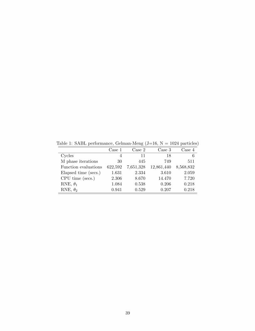
Table 1: SABL performance, Gelman-Meng (J=16, N = 1024 particles)

Case 1 Case 2 Case 3 Case 4

Cycles 4 11 18 6M phase iterations 30 445 749 511Function evaluations 622,592 7,651,328 12,861,440 8,568,832Elapsed time (secs.) 1.631 2.334 3.610 2.059CPU time (secs.) 2.306 8.670 14.470 7.720RNE, θ1 1.084 0.538 0.206 0.218RNE, θ2 0.941 0.529 0.207 0.218

39

Table 2: SABL performance, GARCH (J = 8, N = 512 particles).

Power tempering Data tempering Maximization

Cycles 19 74 25M phase iterations 192 968 200Component evaluations 6,115,983,336 5,004,374,016 6,700,990,464Elapsed time (secs.) 1,116.1 1,006.9 1,211.6CPU time (secs.) 4,427.3 3,779.7 4,545.7

40

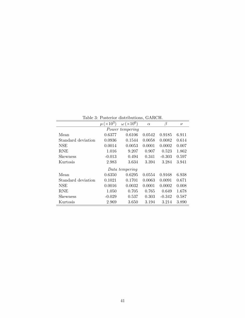
Table 3: Posterior distributions, GARCH.

µ (×103) ω (×106) α β ν

Power temperingMean 0.6377 0.6106 0.0542 0.9185 6.911Standard deviation 0.0936 0.1544 0.0058 0.0082 0.614NSE 0.0014 0.0053 0.0001 0.0002 0.007RNE 1.016 9.207 0.907 0.523 1.862Skewness -0.013 0.494 0.341 -0.303 0.597Kurtosis 2.983 3.634 3.394 3.284 3.941

Data temperingMean 0.6350 0.6295 0.0554 0.9168 6.938Standard deviation 0.1021 0.1701 0.0063 0.0091 0.671NSE 0.0016 0.0032 0.0001 0.0002 0.008RNE 1.050 0.705 0.765 0.649 1.678Skewness -0.029 0.537 0.303 -0.342 0.587Kurtosis 2.969 3.650 3.194 3.214 3.890

41

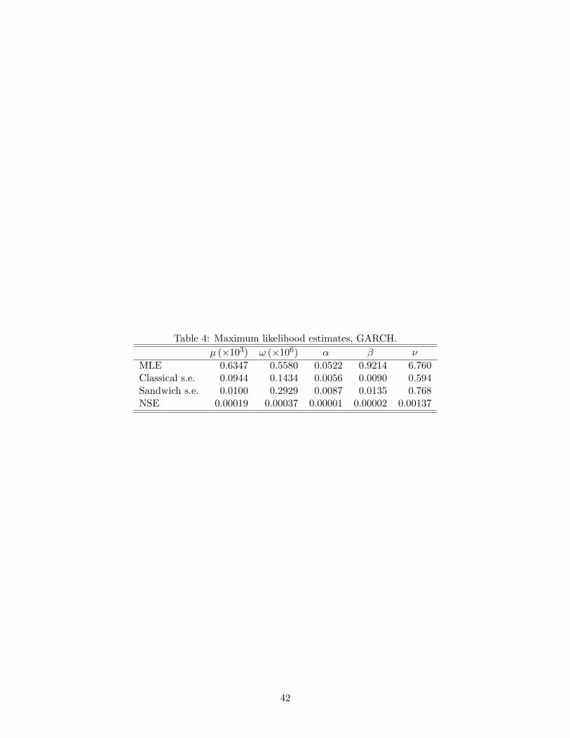
Table 4: Maximum likelihood estimates, GARCH.

µ (×103) ω (×106) α β ν

MLE 0.6347 0.5580 0.0522 0.9214 6.760Classical s.e. 0.0944 0.1434 0.0056 0.0090 0.594Sandwich s.e. 0.0100 0.2929 0.0087 0.0135 0.768NSE 0.00019 0.00037 0.00001 0.00002 0.00137

42

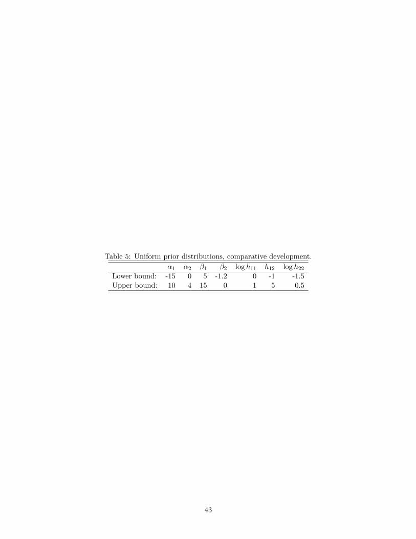
Table 5: Uniform prior distributions, comparative development.

α1 α2 β1 β2 log h11 h12 log h22

Lower bound: -15 0 5 -1.2 0 -1 -1.5Upper bound: 10 4 15 0 1 5 0.5

43

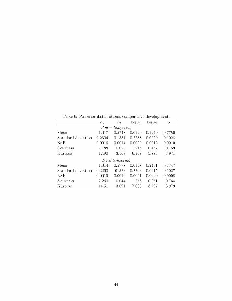
Table 6: Posterior distributions, comparative development.

α2 β2 log σ1 log σ2 ρ

Power temperingMean 1.017 -0.5748 0.0229 0.2240 -0.7750Standard deviation 0.2304 0.1331 0.2288 0.0920 0.1028NSE 0.0016 0.0014 0.0020 0.0012 0.0010Skewness 2.188 0.028 1.216 0.457 0.759Kurtosis 12.90 3.167 6.367 5.885 3.971

Data temperingMean 1.014 -0.5778 0.0198 0.2451 -0.7747Standard deviation 0.2260 01323 0.2263 0.0915 0.1027NSE 0.0019 0.0010 0.0021 0.0009 0.0008Skewness 2.260 0.044 1.258 0.251 0.764Kurtosis 14.51 3.091 7.063 3.797 3.979

44

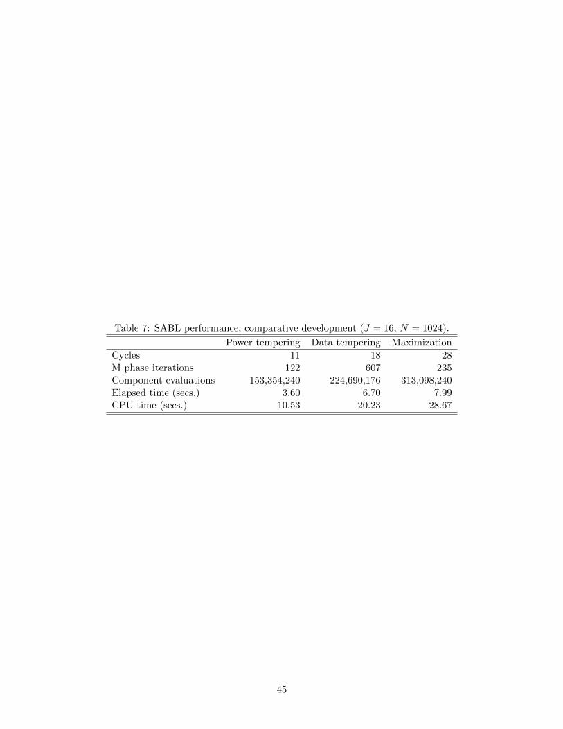
Table 7: SABL performance, comparative development (J = 16, N = 1024).

Power tempering Data tempering Maximization

Cycles 11 18 28M phase iterations 122 607 235Component evaluations 153,354,240 224,690,176 313,098,240Elapsed time (secs.) 3.60 6.70 7.99CPU time (secs.) 10.53 20.23 28.67

45

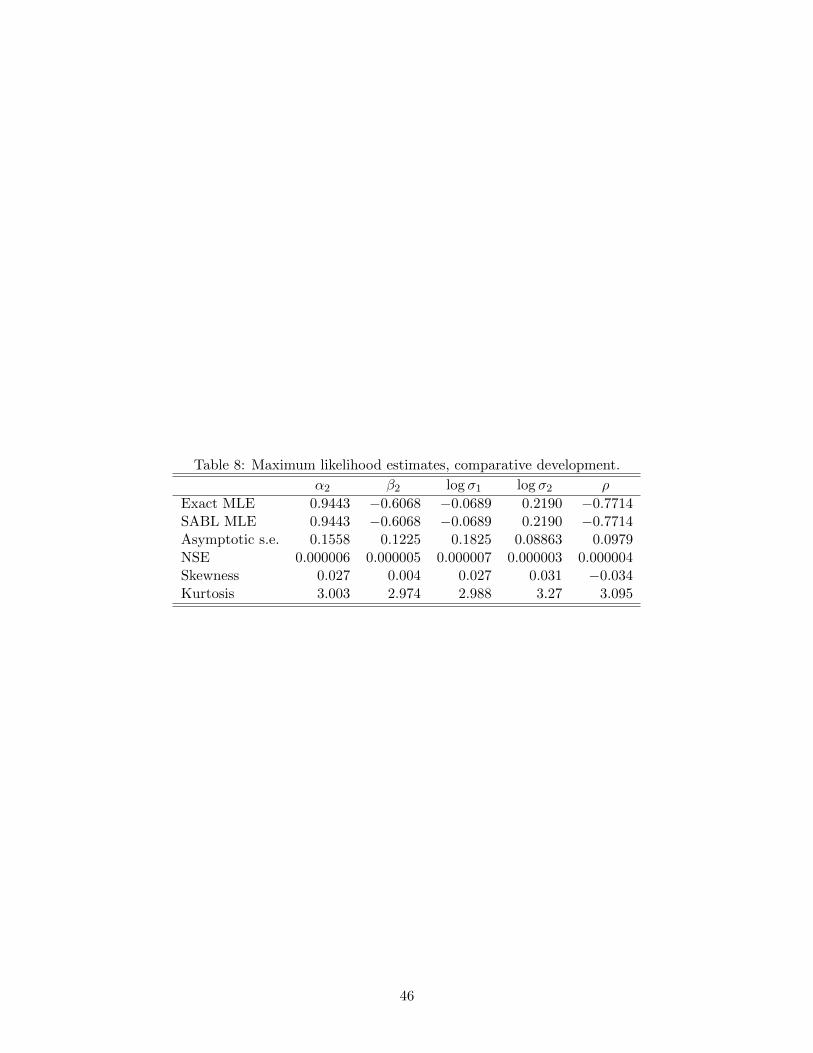
Table 8: Maximum likelihood estimates, comparative development.

α2 β2 log σ1 log σ2 ρ

Exact MLE 0.9443 −0.6068 −0.0689 0.2190 −0.7714SABL MLE 0.9443 −0.6068 −0.0689 0.2190 −0.7714Asymptotic s.e. 0.1558 0.1225 0.1825 0.08863 0.0979NSE 0.000006 0.000005 0.000007 0.000003 0.000004Skewness 0.027 0.004 0.027 0.031 −0.034Kurtosis 3.003 2.974 2.988 3.27 3.095

46

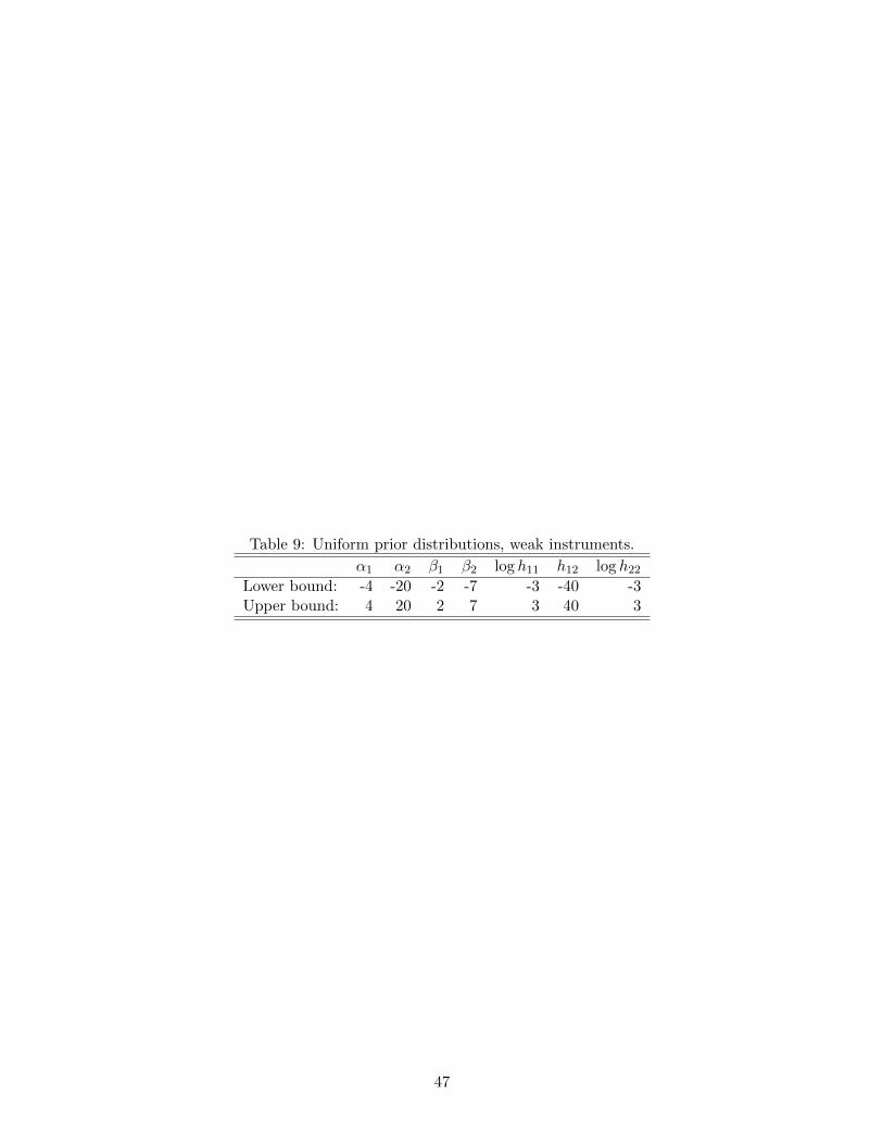
Table 9: Uniform prior distributions, weak instruments.

α1 α2 β1 β2 log h11 h12 log h22

Lower bound: -4 -20 -2 -7 -3 -40 -3Upper bound: 4 20 2 7 3 40 3

47

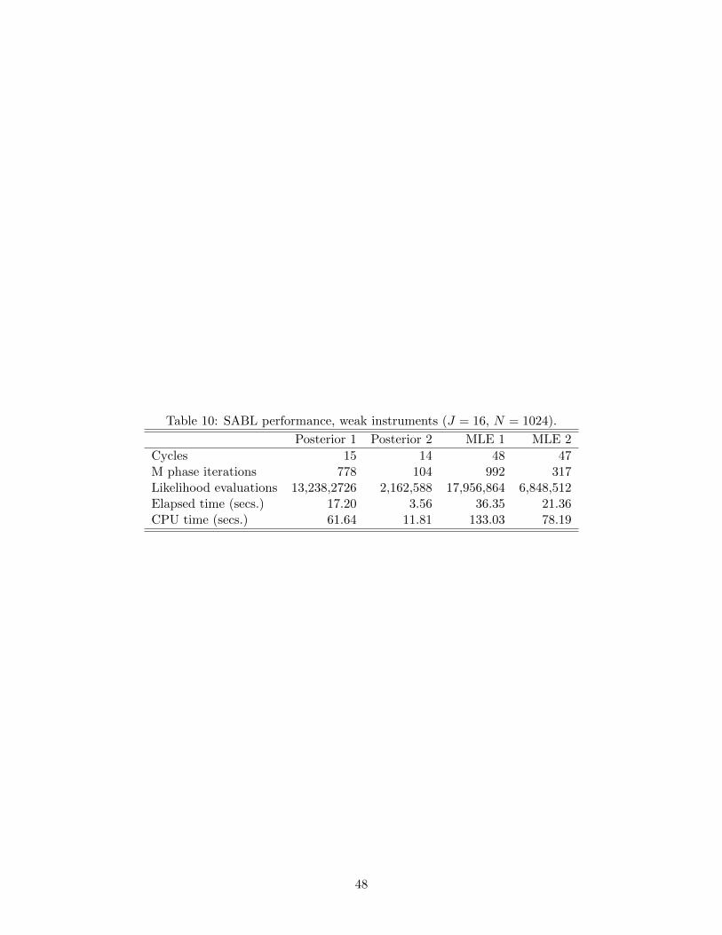
Table 10: SABL performance, weak instruments (J = 16, N = 1024).

Posterior 1 Posterior 2 MLE 1 MLE 2

Cycles 15 14 48 47M phase iterations 778 104 992 317Likelihood evaluations 13,238,2726 2,162,588 17,956,864 6,848,512Elapsed time (secs.) 17.20 3.56 36.35 21.36CPU time (secs.) 61.64 11.81 133.03 78.19

48

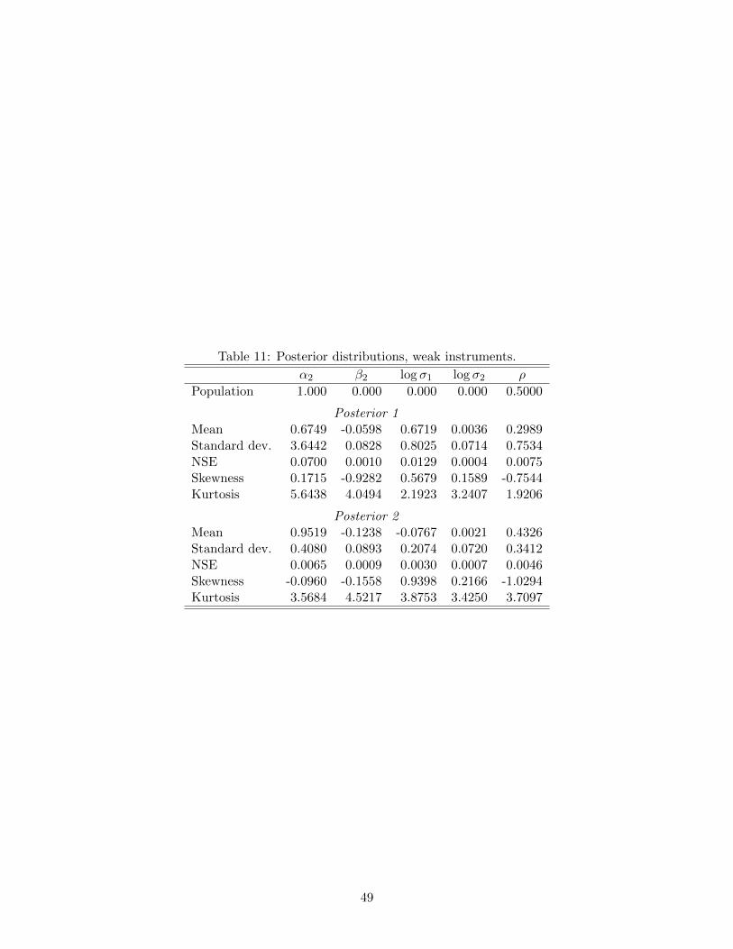
Table 11: Posterior distributions, weak instruments.

α2 β2 log σ1 log σ2 ρ

Population 1.000 0.000 0.000 0.000 0.5000

Posterior 1Mean 0.6749 -0.0598 0.6719 0.0036 0.2989Standard dev. 3.6442 0.0828 0.8025 0.0714 0.7534NSE 0.0700 0.0010 0.0129 0.0004 0.0075Skewness 0.1715 -0.9282 0.5679 0.1589 -0.7544Kurtosis 5.6438 4.0494 2.1923 3.2407 1.9206

Posterior 2Mean 0.9519 -0.1238 -0.0767 0.0021 0.4326Standard dev. 0.4080 0.0893 0.2074 0.0720 0.3412NSE 0.0065 0.0009 0.0030 0.0007 0.0046Skewness -0.0960 -0.1558 0.9398 0.2166 -1.0294Kurtosis 3.5684 4.5217 3.8753 3.4250 3.7097

49

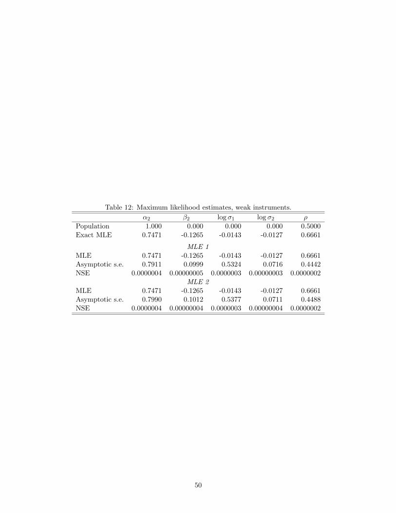
Table 12: Maximum likelihood estimates, weak instruments.

α2 β2 log σ1 log σ2 ρ

Population 1.000 0.000 0.000 0.000 0.5000Exact MLE 0.7471 -0.1265 -0.0143 -0.0127 0.6661

MLE 1MLE 0.7471 -0.1265 -0.0143 -0.0127 0.6661Asymptotic s.e. 0.7911 0.0999 0.5324 0.0716 0.4442NSE 0.0000004 0.00000005 0.0000003 0.00000003 0.0000002

MLE 2MLE 0.7471 -0.1265 -0.0143 -0.0127 0.6661Asymptotic s.e. 0.7990 0.1012 0.5377 0.0711 0.4488NSE 0.0000004 0.00000004 0.0000003 0.00000004 0.0000002

50

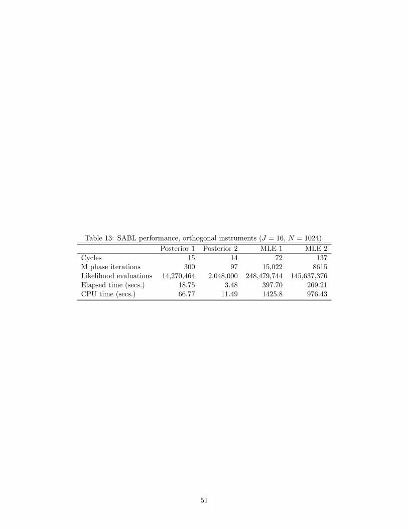
Table 13: SABL performance, orthogonal instruments (J = 16, N = 1024).

Posterior 1 Posterior 2 MLE 1 MLE 2

Cycles 15 14 72 137M phase iterations 300 97 15,022 8615Likelihood evaluations 14,270,464 2,048,000 248,479,744 145,637,376Elapsed time (secs.) 18.75 3.48 397.70 269.21CPU time (secs.) 66.77 11.49 1425.8 976.43

51

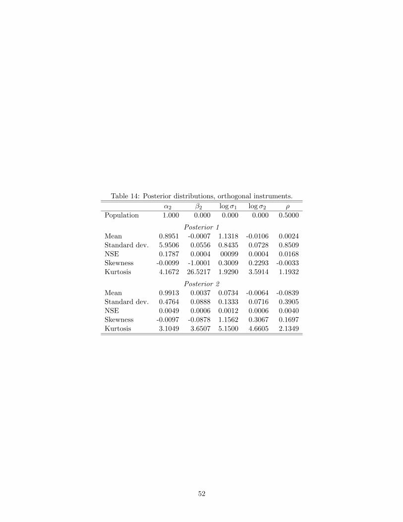
Table 14: Posterior distributions, orthogonal instruments.

α2 β2 log σ1 log σ2 ρ

Population 1.000 0.000 0.000 0.000 0.5000

Posterior 1Mean 0.8951 -0.0007 1.1318 -0.0106 0.0024Standard dev. 5.9506 0.0556 0.8435 0.0728 0.8509NSE 0.1787 0.0004 00099 0.0004 0.0168Skewness -0.0099 -1.0001 0.3009 0.2293 -0.0033Kurtosis 4.1672 26.5217 1.9290 3.5914 1.1932

Posterior 2Mean 0.9913 0.0037 0.0734 -0.0064 -0.0839Standard dev. 0.4764 0.0888 0.1333 0.0716 0.3905NSE 0.0049 0.0006 0.0012 0.0006 0.0040Skewness -0.0097 -0.0878 1.1562 0.3067 0.1697Kurtosis 3.1049 3.6507 5.1500 4.6605 2.1349

52

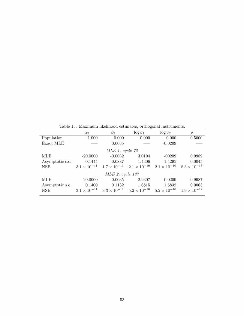
Table 15: Maximum likelihood estimates, orthogonal instruments.

α2 β2 log σ1 log σ2 ρ

Population 1.000 0.000 0.000 0.000 0.5000Exact MLE —– 0.0035 —– -0.0209 —–

MLE 1, cycle 72MLE -20.0000 -0.0032 3.0194 -00209 0.9989Asymptotic s.e. 0.1444 0.0887 1.4306 1.4295 0.0045NSE 3.1× 10−11 1.7× 10−11 2.1× 10−10 2.1× 10−10 8.3× 10−13

MLE 2, cycle 137MLE 20.0000 0.0035 2.9307 -0.0209 -0.9987Asymptotic s.e. 0.1400 0.1132 1.6815 1.6832 0.0063NSE 3.1× 10−11 3.3× 10−11 5.2× 10−10 5.2× 10−10 1.9× 10−12

53

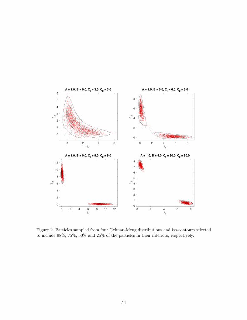
0 2 4 6

1

0

1

2

3

4

5

6

2

A = 1.0, B = 0.0, C1 = 3.0, C

2 = 3.0

0 2 4 6 8

1

0

2

4

6

8

2

A = 1.0, B = 0.0, C1 = 6.0, C

2 = 6.0

0 2 4 6 8 10 12

1

0

2

4

6

8

10

12

2

A = 1.0, B = 0.0, C1 = 9.0, C

2 = 9.0

0 2 4 6 8

1

0

1

2

3

4

5

6

7

8

2

A = 1.0, B = 4.0, C1 = 80.0, C

2 = 80.0

Figure 1: Particles sampled from four Gelman-Meng distributions and iso-contours selectedto include 98%, 75%, 50% and 25% of the particles in their interiors, respectively.

54

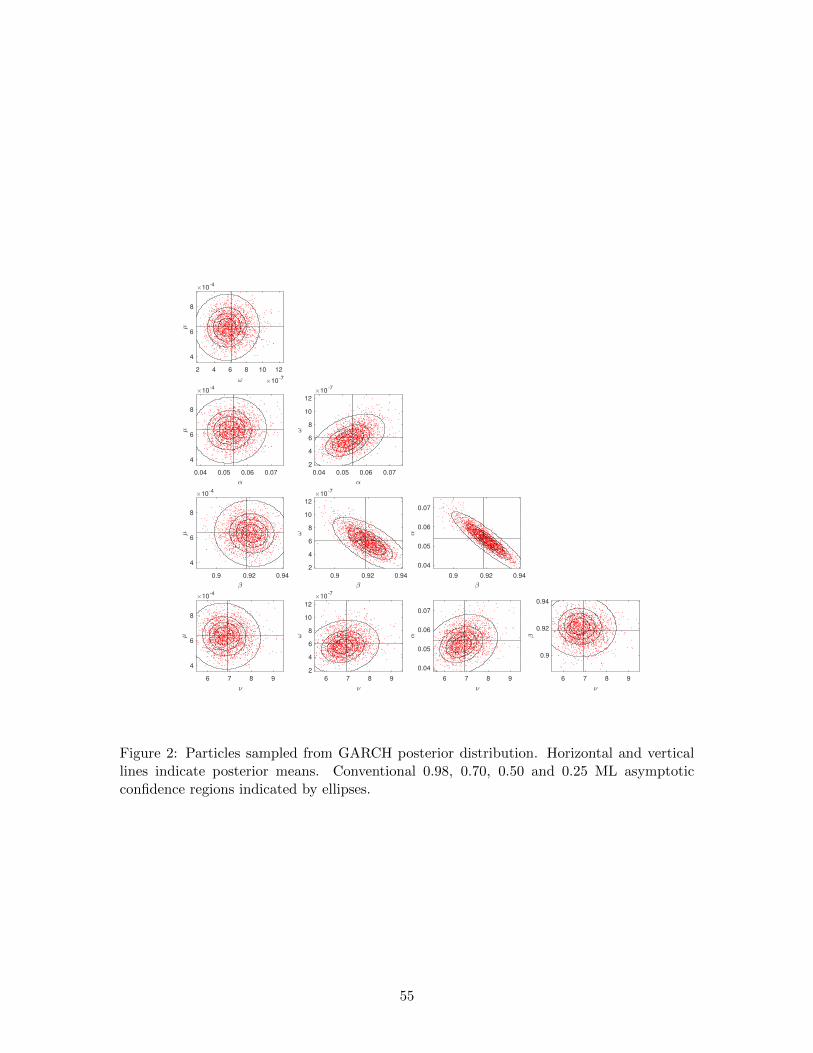
2 4 6 8 10 12

10-7

4

6

8

10-4

0.04 0.05 0.06 0.07

4

6

8

10-4

0.04 0.05 0.06 0.07

2

4

6

8

10

12

10-7

0.9 0.92 0.94

4

6

8

10-4

0.9 0.92 0.94

2

4

6

8

10

12

10-7

0.9 0.92 0.94

0.04

0.05

0.06

0.07

6 7 8 9

4

6

8

10-4

6 7 8 9

2

4

6

8

10

12

10-7

6 7 8 9

0.04

0.05

0.06

0.07

6 7 8 9

0.9

0.92

0.94

Figure 2: Particles sampled from GARCH posterior distribution. Horizontal and verticallines indicate posterior means. Conventional 0.98, 0.70, 0.50 and 0.25 ML asymptoticconfidence regions indicated by ellipses.

55

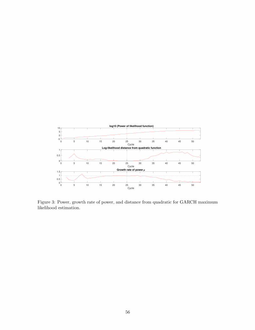
0 5 10 15 20 25 30 35 40 45 50

Cycle

-5

0

5

10log10 (Power of likelihood function)

0 5 10 15 20 25 30 35 40 45 50

Cycle

0

0.5

1Log-likelihood distance from quadratic function

0 5 10 15 20 25 30 35 40 45 50

Cycle

0

0.5

1

1.5Growth rate of power

Figure 3: Power, growth rate of power, and distance from quadratic for GARCH maximumlikelihood estimation.

56

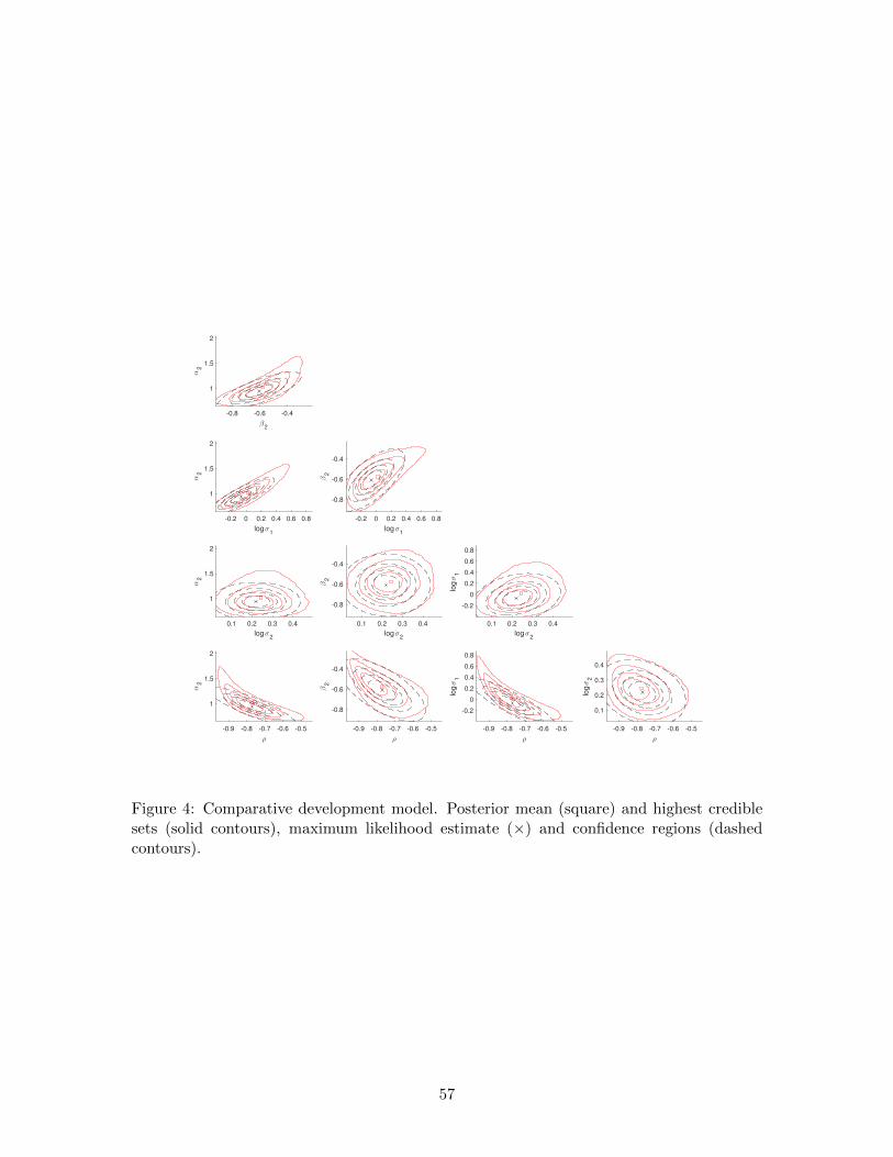
-0.8 -0.6 -0.4

2

1

1.5

2

2

-0.2 0 0.2 0.4 0.6 0.8

log1

1

1.5

2

2

-0.2 0 0.2 0.4 0.6 0.8

log1

-0.8

-0.6

-0.4

2

0.1 0.2 0.3 0.4

log2

1

1.5

2

2

0.1 0.2 0.3 0.4

log2

-0.8

-0.6

-0.4

2

0.1 0.2 0.3 0.4

log2

-0.2

0

0.2

0.4

0.6

0.8

log

1

-0.9 -0.8 -0.7 -0.6 -0.5

1

1.5

2

2

-0.9 -0.8 -0.7 -0.6 -0.5

-0.8

-0.6

-0.4

2

-0.9 -0.8 -0.7 -0.6 -0.5

-0.2

0

0.2

0.4

0.6

0.8

log

1

-0.9 -0.8 -0.7 -0.6 -0.5

0.1

0.2

0.3

0.4

log

2

Figure 4: Comparative development model. Posterior mean (square) and highest crediblesets (solid contours), maximum likelihood estimate (×) and confidence regions (dashedcontours).

57

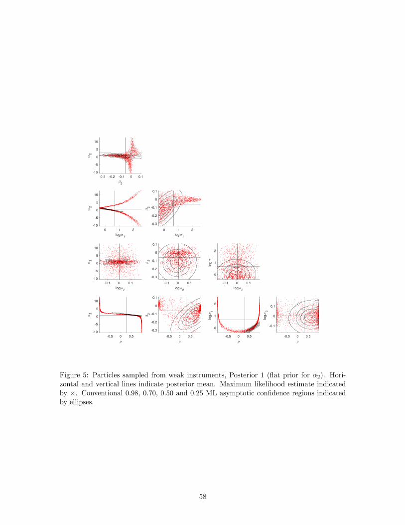
-0.3 -0.2 -0.1 0 0.1

2

-10

-5

0

5

10

2

0 1 2

log1

-10

-5

0

5

10

2

0 1 2

log1

-0.3

-0.2

-0.1

0

0.1

2

-0.1 0 0.1

log2

-10

-5

0

5

10

2

-0.1 0 0.1

log2

-0.3

-0.2

-0.1

0

0.1

2

-0.1 0 0.1

log2

0

1

2

log

1

-0.5 0 0.5

-10

-5

0

5

10

2

-0.5 0 0.5

-0.3

-0.2

-0.1

0

0.1

2

-0.5 0 0.5

0

1

2

log

1

-0.5 0 0.5

-0.1

0

0.1

log

2

Figure 5: Particles sampled from weak instruments, Posterior 1 (flat prior for α2). Hori-zontal and vertical lines indicate posterior mean. Maximum likelihood estimate indicatedby ×. Conventional 0.98, 0.70, 0.50 and 0.25 ML asymptotic confidence regions indicatedby ellipses.

58

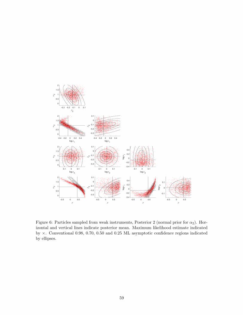
-0.3 -0.2 -0.1 0 0.1

2

0

0.5

1

1.5

2

2

-0.4 -0.2 0 0.2 0.4

log1

0

0.5

1

1.5

2

2

-0.4 -0.2 0 0.2 0.4

log1

-0.3

-0.2

-0.1

0

0.1

2

-0.1 0 0.1

log2

0

0.5

1

1.5

2

2

-0.1 0 0.1

log2

-0.3

-0.2

-0.1

0

0.1

2

-0.1 0 0.1

log2

-0.4

-0.2

0

0.2

0.4

log

1

-0.5 0 0.5

0

0.5

1

1.5

2

2

-0.5 0 0.5

-0.3

-0.2

-0.1

0

0.1

2

-0.5 0 0.5-0.4

-0.2

0

0.2

0.4

log

1

-0.5 0 0.5

-0.1

0

0.1

log

2

Figure 6: Particles sampled from weak instruments, Posterior 2 (normal prior for α2). Hor-izontal and vertical lines indicate posterior mean. Maximum likelihood estimate indicatedby ×. Conventional 0.98, 0.70, 0.50 and 0.25 ML asymptotic confidence regions indicatedby ellipses.

59

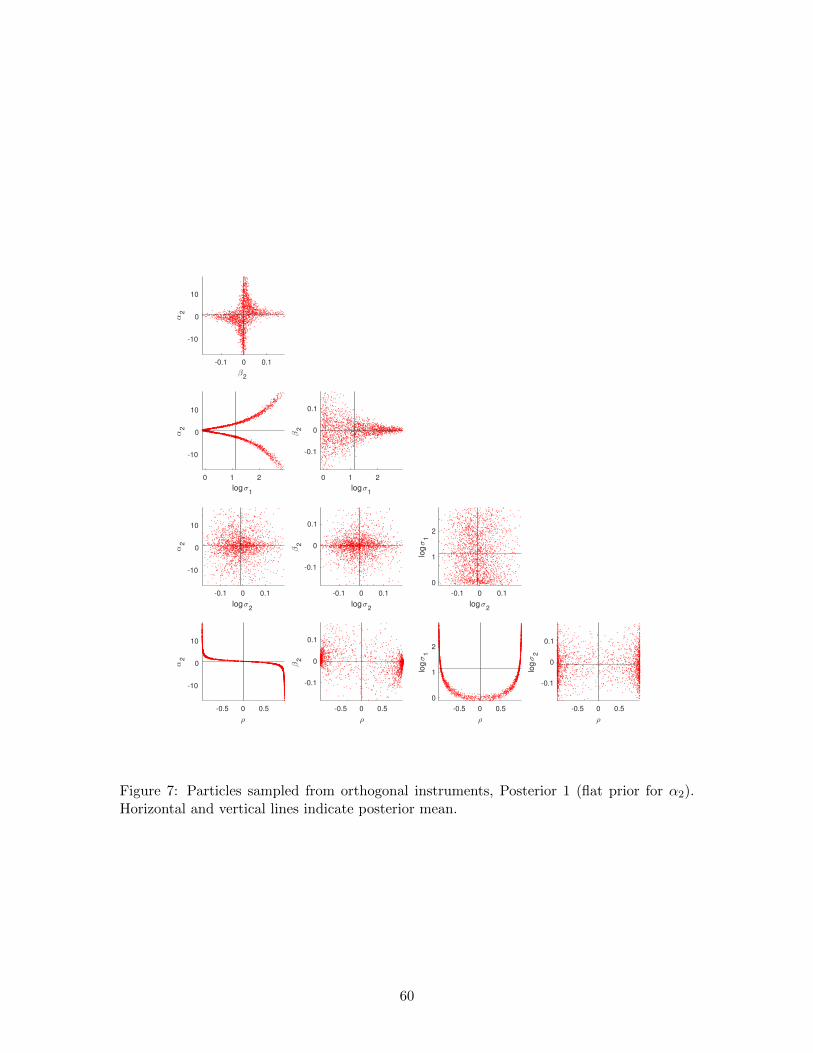
-0.1 0 0.1

2

-10

0

10

2

0 1 2

log1

-10

0

10

2

0 1 2

log1

-0.1

0

0.1

2

-0.1 0 0.1

log2

-10

0

10

2

-0.1 0 0.1

log2

-0.1

0

0.1

2

-0.1 0 0.1

log2

0

1

2

log

1

-0.5 0 0.5

-10

0

10

2

-0.5 0 0.5

-0.1

0

0.1

2

-0.5 0 0.5

0

1

2

log

1

-0.5 0 0.5

-0.1

0

0.1

log

2

Figure 7: Particles sampled from orthogonal instruments, Posterior 1 (flat prior for α2).Horizontal and vertical lines indicate posterior mean.

60

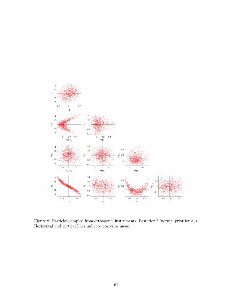
-0.2 0 0.2

2

0

0.5

1

1.5

2

2

0 0.2 0.4

log1

0

0.5

1

1.5

2

2

0 0.2 0.4

log1

-0.2

-0.1

0

0.1

0.2

2

-0.1 0 0.1

log2

0

0.5

1

1.5

2

2

-0.1 0 0.1

log2

-0.2

-0.1

0

0.1

0.2

2

-0.1 0 0.1

log2

0

0.2

0.4

log

1

-0.5 0 0.5

0

0.5

1

1.5

2

2

-0.5 0 0.5

-0.2

-0.1

0

0.1

0.2

2

-0.5 0 0.5

0

0.2

0.4

log

1

-0.5 0 0.5

-0.1

0

0.1

log

2

Figure 8: Particles sampled from orthogonal instruments, Posterior 2 (normal prior for α2).Horizontal and vertical lines indicate posterior mean.

61