Sensorless PMSM Field-Oriented Control · Data types ..... 14 3.2. Scaling of analog quantities ... Sensorless PMSM Field-Oriented Control, Design Reference Manual, Rev. 1, 02/2016

© 2016 Freescale Semiconductor, Inc. All rights reserved.

Sensorless PMSM Field-Oriented Control

1. Introduction Sinusoidal Permanent Magnet Synchronous Motors (PMSM) are getting more and more popular, replacing brushed DC, universal, and other motors in a wide application area. Here are some of the reasons:

• Better reliability when compared to brushed DC motors.

• Better efficiency when compared to AC Induction Motors (ACIM) because the rotor flux is generated by magnets.

• Lower acoustic noise. • Smaller dimensions when compared to ACIM.

The disadvantage of the PMSM drives is the need for a more sophisticated electronic circuit. Nowadays, most applications need electronic speed or torque regulation and other features with the necessity of electronic control. When a system with electronic control is used, it only takes small system cost increase to implement more advanced drives, such as the sinusoidal PMSM with a digitally-controlled switching inverter and a DC-bus circuit. It is only necessary to have a cost-effective controller with a good calculation performance. PMSMs are used in domestic appliances (such as refrigerators, washing machines, dishwashers), pumps, compressors, fans, and other appliances that require high reliability and efficiency.

Freescale Semiconductor, Inc. Document Number: DRM148

Design Reference Manual Rev. 1 , 02/2016

Contents 1. Introduction ........................................................................ 1 2. PMSM Control Theory ...................................................... 2

2.1. 3-phase PMSM ....................................................... 2 2.2. Mathematical description of PMSM ....................... 2 2.3. PMSM field-oriented control .................................. 6

3. Software Design ............................................................... 14 3.1. Data types ............................................................. 14 3.2. Scaling of analog quantities .................................. 15 3.3. Application overview ............................................ 16 3.4. Synchronizing motor-control algorithms .............. 17 3.5. Calling algorithms ................................................. 18 3.6. Main state machine ............................................... 19 3.7. Motor state machine .............................................. 22 3.8. Sensorless PMSM control ..................................... 27

4. Acronyms and Abbreviations ........................................... 38 5. List of Symbols ................................................................ 39 6. Revision History .............................................................. 40

PMSM Control Theory

Sensorless PMSM Field-Oriented Control, Design Reference Manual, Rev. 1, 02/2016 2 Freescale Semiconductor, Inc.

The control algorithms are divided into two general groups. The first group is called scalar control (SC). The constant Volt per Hertz control represents the scalar control. The other group is called vector control (VC), or field-oriented control (FOC). The FOC technique brings overall improvements in drive performance when compared to the scalar control (higher efficiency, full torque control from zero to nominal motor speed, decoupled control of flux and torque, improved dynamics, etc.). For the PMSM control, it is necessary to know the exact rotor position. This application uses special algorithms to estimate the speed and position instead of using a physical position sensor.

The software algorithms consist of software blocks (such as the state machine, motor-control drivers (MCDRV), and motor-control application tuning (MCAT) tool) supporting online application tuning. This design reference manual describes the basic motor theory and software design.

2. PMSM Control Theory

2.1. 3-phase PMSM The PMSM is a rotating electric machine with a standard 3-phase stator, like that of an induction motor; the rotor has surface-mounted permanent magnets. See this figure:

Figure 1. PMSM cross-section

In this aspect, the PMSM is equivalent to induction motors, where the air gap magnetic field is produced by permanent magnets, so the rotor magnetic field is constant. The PMSMs offer a number of advantages in designing modern motion-control systems. The use of a permanent magnet to generate a substantial air gap magnetic flux makes it possible to design highly efficient PMSMs.

2.2. Mathematical description of PMSM There are several PMSM models. The model used for the vector control design is obtained using the space-vector theory. The 3-phase motor quantities (such as voltages, currents, magnetic flux, etc.) are expressed in terms of complex space vectors. Such model is valid for any instantaneous variation of voltage and current, and adequately describes the performance of the machine under both the steady-state and transient operations.

PMSM Control Theory

Sensorless PMSM Field-Oriented Control, Design Reference Manual, Rev. 1, 02/2016 Freescale Semiconductor, Inc. 3

Complex space vectors are described using only two orthogonal axes. Using the 2-phase motor model reduces the number of equations and simplifies the control design.

2.2.1. Space vector definitions Assume that isa, isb, and isc are the instantaneous balanced 3-phase stator currents:

Eq. 1 𝒊𝒊𝒔𝒔𝒔𝒔 + 𝒊𝒊𝒔𝒔𝒔𝒔 + 𝒊𝒊𝒔𝒔𝒔𝒔 = 𝟎𝟎

Then the stator-current space vector can be defined as:

Eq. 2 𝒊𝒊𝒔𝒔� = 𝒌𝒌(𝒊𝒊𝒔𝒔𝒔𝒔 + 𝒔𝒔𝒊𝒊𝒔𝒔𝒔𝒔 + 𝒔𝒔𝟐𝟐𝒊𝒊𝒔𝒔𝒔𝒔)

where a and a2 are the spatial operators 𝑎𝑎 = 𝑒𝑒𝑗𝑗2𝜋𝜋/3 , 𝑎𝑎2 = 𝑒𝑒𝑗𝑗4𝜋𝜋/3, and k is the transformation constant k=2/3. Figure 2 shows the stator-current space vector projection. The space vector defined by Eq. 3 can be expressed using the 2-axis theory. The real part of the space vector is equal to the instantaneous value of the direct-axis stator current component isα, and its imaginary part is equal to the quadrature-axis stator current component isβ. Thus, the stator-current space vector in the stationary reference frame attached to the stator is expressed as:

Eq. 3 𝒊𝒊𝒔𝒔� = 𝒊𝒊𝒔𝒔𝒔𝒔 + 𝒋𝒋𝒊𝒊𝒔𝒔𝒔𝒔

Figure 2. Stator current space vector and its projection

In symmetrical 3-phase machines, the direct and quadrature axis stator currents (isα , isβ) are fictitious quadrature-phase (2-phase) current components, which are related to the actual 3-phase stator currents as:

Eq. 4 𝒊𝒊𝒔𝒔𝒔𝒔 = 𝒌𝒌 �𝒊𝒊𝒔𝒔𝒔𝒔 −𝟏𝟏𝟐𝟐𝒊𝒊𝒔𝒔𝒔𝒔 −

𝟏𝟏𝟐𝟐𝒊𝒊𝒔𝒔𝒔𝒔�

isb

iscisa

is

isb

isc

isα

isβ

phase-a, α

βphase-b

phase-c

_

PMSM Control Theory


Eq. 5 𝒊𝒊𝒔𝒔𝒔𝒔 = 𝒌𝒌 √𝟑𝟑𝟐𝟐

(𝒊𝒊𝒔𝒔𝒔𝒔−𝒊𝒊𝒔𝒔𝒔𝒔)

where k=2/3 is the transformation constant, so that the final equation is:

Eq. 6 𝒊𝒊𝒔𝒔𝒔𝒔 = 𝟏𝟏√𝟑𝟑

(𝒊𝒊𝒔𝒔𝒔𝒔−𝒊𝒊𝒔𝒔𝒔𝒔)

The space vectors of other motor quantities (such as voltages, currents, magnetic fluxes) can be defined in the same way as the stator-current space vector.

2.2.2. PMSM model The symmetrical 3-phase smooth-air-gap machine with sinusoidally-distributed windings is taken as the description of a PMSM. The voltage equations of the stator in the instantaneous form are expressed as:

Eq. 7 𝒖𝒖𝑺𝑺𝑺𝑺 = 𝑹𝑹𝑺𝑺𝒊𝒊𝑺𝑺𝑺𝑺 + 𝒅𝒅𝒅𝒅𝒅𝒅𝝍𝝍𝑺𝑺𝑺𝑺



where uSA, uSB, and uSC are the instantaneous values of stator voltages, iSA, iSB, and iSC are the instantaneous values of stator currents, and ψSA, ψSB, ψSC are the instantaneous values of the stator flux linkages in phases SA, SB, and SC. Due to a large number of equations in the instantaneous form, (Eq. 7, Eq. 8, and Eq. 9), it is better to rewrite the instantaneous equations using the 2-axis theory (Clarke transformation). The PMSM is then expressed as:

Eq. 10 𝒖𝒖𝑺𝑺𝒔𝒔 = 𝑹𝑹𝑺𝑺𝒊𝒊𝑺𝑺𝒔𝒔 + 𝒅𝒅𝒅𝒅𝒅𝒅𝝍𝝍𝑺𝑺𝒔𝒔

Eq. 11 𝒖𝒖𝑺𝑺𝒔𝒔 = 𝑹𝑹𝑺𝑺𝒊𝒊𝑺𝑺𝒔𝒔 + 𝒅𝒅𝒅𝒅𝒅𝒅𝝍𝝍𝑺𝑺𝒔𝒔

Eq. 12 𝝍𝝍𝑺𝑺𝒔𝒔 = 𝑳𝑳𝑺𝑺𝒊𝒊𝑺𝑺𝒔𝒔 + 𝝍𝝍𝑴𝑴 𝒔𝒔𝒄𝒄𝒔𝒔𝜣𝜣𝒓𝒓

Eq. 13 𝝍𝝍𝑺𝑺𝒔𝒔 = 𝑳𝑳𝑺𝑺𝒊𝒊𝑺𝑺𝒔𝒔 + 𝝍𝝍𝑴𝑴 𝒔𝒔𝒊𝒊𝒔𝒔𝜣𝜣𝒓𝒓

Eq. 14 𝒅𝒅𝒅𝒅𝒅𝒅𝒅𝒅

= 𝒑𝒑𝑱𝑱�𝟐𝟐𝟑𝟑𝒑𝒑�𝝍𝝍𝑺𝑺𝒔𝒔𝒊𝒊𝑺𝑺𝒔𝒔 − 𝝍𝝍𝑺𝑺𝒔𝒔𝒊𝒊𝑺𝑺𝒔𝒔�−𝑻𝑻𝑳𝑳�

For a glossary of symbols, see Table 3.

The equations Eq. 10 to Eq. 14 represent the model of a PMSM in the stationary frame α, β, fixed to the stator.

Besides the stationary reference frame attached to the stator, the motor model voltage space vector equations can be formulated in a general reference frame that rotates at a general speed ωg. Using a general reference frame with the direct and quadrature axes (x and y) rotating at a general instantaneous speed ωg=dθg/dt (as shown in Figure 3) where θg is the angle between the direct axis of the stationary reference frame (α) attached to the stator and the real axis (x) of the general reference frame, Eq. 15 defines the stator-current space vector in a general reference frame as:

Eq. 15 𝒊𝒊𝒔𝒔𝒔𝒔�� = 𝒊𝒊𝒔𝒔�𝒆𝒆−𝒋𝒋𝜣𝜣𝒔𝒔 = 𝒊𝒊𝒔𝒔𝒔𝒔 + 𝒋𝒋𝒊𝒊𝒔𝒔𝒔𝒔

PMSM Control Theory


Figure 3. Application of general reference frame

The stator-voltage and flux-linkage space vectors can be obtained similarly in the general reference frame.

Similar considerations are held for the space vectors of the rotor voltages, currents, and flux linkages. The real axis (rα) of the reference frame attached to the rotor is displaced from the direct axis of the stator reference frame by the rotor angle θr. The angle between the real axis (x) of the general reference frame and the real axis of the reference frame rotating with the rotor (rα) is θg-θr. In the general reference frame, the space vector of the rotor currents is expressed as:

Eq. 16 𝒊𝒊𝒓𝒓𝒔𝒔�� = 𝒊𝒊𝒓𝒓�𝒆𝒆−𝒋𝒋�𝜣𝜣𝒔𝒔−𝜣𝜣𝒓𝒓� = 𝒊𝒊𝒓𝒓𝒔𝒔 + 𝒋𝒋𝒊𝒊𝒓𝒓𝒔𝒔

where 𝚤𝚤𝑟𝑟� is the space vector of the rotor current in the rotor reference frame.

The space vectors of the rotor voltages and rotor flux linkages in the general reference frame can be expressed similarly.

The motor model voltage equations in the general reference frame can be expressed using the introduced transformations of the motor quantities from one reference frame to the general reference frame. The PMSM model is often used in vector-control algorithms. The aim of the vector control is to implement the control schemes that produce high-dynamic performance and are similar to those used to control DC machines. To achieve this, the reference frames must be aligned with the stator flux-linkage space vector, the rotor flux-linkage space vector, or the magnetizing space vector. The most popular reference frame is the reference frame attached to the rotor flux-linkage space vector with the direct axis (d) and the quadrature axis (q).

Transformed into the d, q coordinates, the motor model is:

Eq. 17 𝒖𝒖𝑺𝑺𝒅𝒅 = 𝑹𝑹𝑺𝑺𝒊𝒊𝑺𝑺𝒅𝒅 + 𝒅𝒅𝒅𝒅𝒅𝒅𝝍𝝍𝑺𝑺𝒅𝒅 − 𝒅𝒅𝑭𝑭𝝍𝝍𝑺𝑺𝑺𝑺

Eq. 18 𝒖𝒖𝑺𝑺𝑺𝑺 = 𝑹𝑹𝑺𝑺𝒊𝒊𝑺𝑺𝑺𝑺 + 𝒅𝒅𝒅𝒅𝒅𝒅𝝍𝝍𝑺𝑺𝑺𝑺 − 𝒅𝒅𝑭𝑭𝝍𝝍𝑺𝑺𝒅𝒅

Eq. 19 𝝍𝝍𝑺𝑺𝒅𝒅 = 𝑳𝑳𝑺𝑺𝒊𝒊𝑺𝑺𝒅𝒅 + 𝝍𝝍𝑴𝑴

Eq. 20 𝝍𝝍𝑺𝑺𝑺𝑺 = 𝑳𝑳𝑺𝑺𝒊𝒊𝑺𝑺𝑺𝑺

isα

isβ

α

β

x

y

θg

ωg

is, isg

_ _

PMSM Control Theory



= 𝒑𝒑𝑱𝑱�𝟐𝟐𝟑𝟑𝒑𝒑�𝝍𝝍𝑺𝑺𝒅𝒅𝒊𝒊𝑺𝑺𝒅𝒅 − 𝝍𝝍𝑺𝑺𝑺𝑺𝒊𝒊𝑺𝑺𝑺𝑺�−𝑻𝑻𝑳𝑳�

Considering that the below base speed is isd=0, Eq. 21 can be reduced as:


= 𝒑𝒑𝑱𝑱�𝟐𝟐𝟑𝟑𝒑𝒑�𝝍𝝍𝑴𝑴𝒊𝒊𝑺𝑺𝑺𝑺�−𝑻𝑻𝑳𝑳�

In Eq. 22, the torque is dependent and can be directly controlled by the current isq only.

2.3. PMSM field-oriented control

2.3.1. Fundamental principle of field-oriented control (FOC) High-performance motor control is characterized by smooth rotation over the entire speed range of the motor, full torque control at zero speed, and fast accelerations and decelerations. To achieve such control, use the FOC techniques for 3-phase AC motors. The basic idea of the FOC algorithm is to decompose the stator current into the magnetic field-generating part and the torque-generating part. Both components can be controlled separately after the decomposition. The structure of the motor controller is then as simple as that for separately excited DC motors.

Figure 4 shows the basic structure of the vector-control algorithm for the PMSM. To perform the vector control, follow these steps:

1. Measure the motor quantities (phase voltages and currents). 2. Transform them into the 2-phase system (α, β) using Clarke transformation. 3. Calculate the rotor-flux space vector magnitude and position angle. 4. Transform the stator currents into the d, q reference frame using Park transformation. 5. The stator current torque-producing (isq) and flux-producing (isd) components are controlled

separately. 6. The stator-voltage space vector is transformed by the inverse Park transformation back from the

d, q reference frame into the 2-phase system fixed with the stator. 7. The 3-phase output voltage is generated using the space vector modulation.

To decompose the currents into torque-producing and flux-producing components (isd, isq), you must know the rotor position. This requires an accurate sensing of the rotor position and velocity information. The incremental encoders or resolvers attached to the rotor are mostly used as position transducers for vector-control drives. In some applications, the use of speed/position sensors is not wanted. The aim is not to measure the speed/position directly, but to employ some indirect techniques to estimate the rotor position instead. The algorithms that do not employ speed sensors are called “sensorless control”.

PMSM Control Theory


Figure 4. FOC transformations

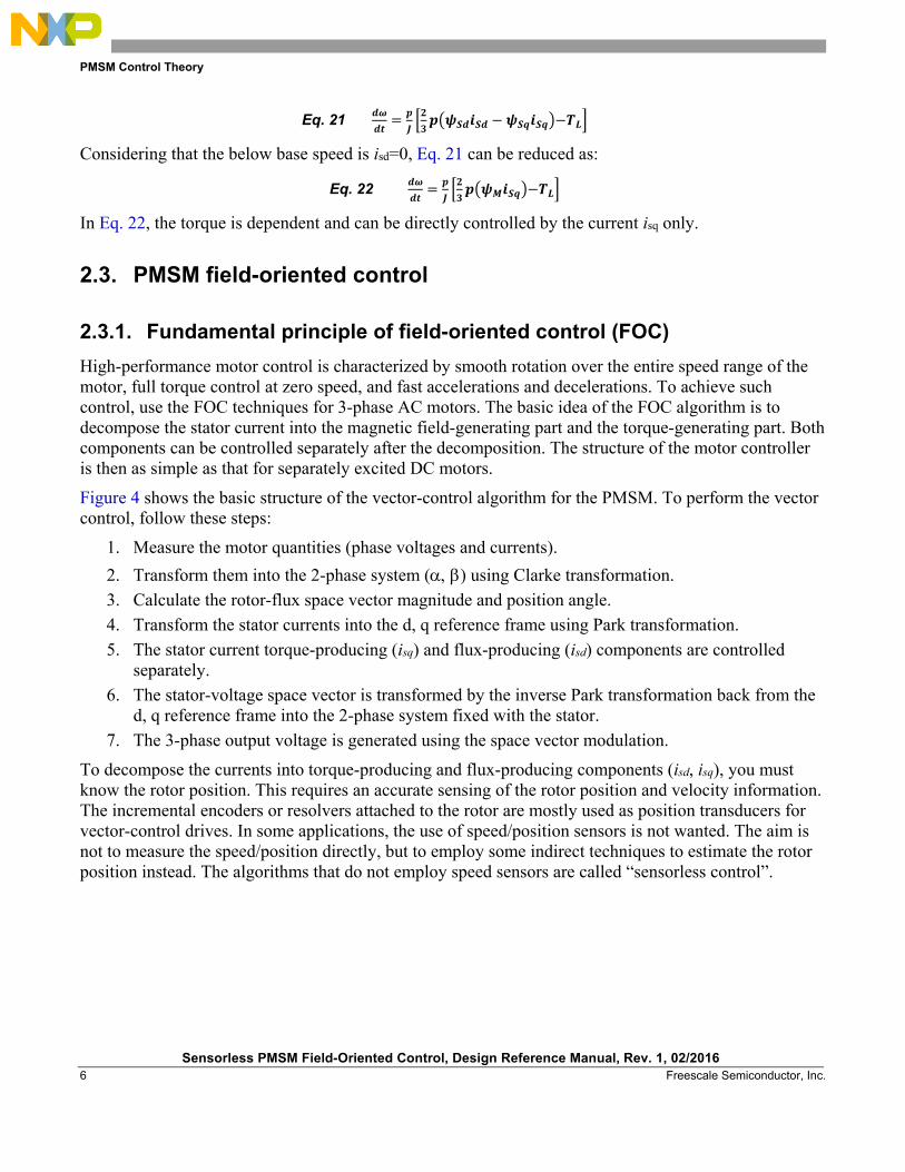
2.3.2. FOC algorithm description The overview block diagram of the implemented control algorithm is shown in Figure 5. As with the other FOC techniques, it is able to control the field and torque of the motor separately. The aim of the control is to regulate motor speed. The speed command value is set by the high-level control. The algorithm is executed in two control loops. The fast inner control loop is executed with a period of 100 µs. The slow outer control loop is executed with a period of 1 ms.

To achieve the goal of the PMSM control, the algorithm uses feedback signals. The essential feedback signals are the 3-phase stator current and DC-bus voltage. The regulator output is used for the stator voltage. To operate properly, the presented control structure requires either the position and speed sensors on the motor shaft or an advanced algorithm to estimate the position and speed.

The fast control loop executes these two independent current-control loops: • The direct-axis current (isd) PI controllers—the direct-axis current (isd) is used to control the rotor

magnetizing flux. • The quadrature-axis current (isq) PI controllers—the quadrature-axis current corresponds to the

motor torque.

Phase APhase BPhase C

α

β

Phase APhase BPhase C

d

q

d

q

α

β3-Phase

to2-Phase

Stationaryto

RotatingSVM

3-PhaseSystem

3-PhaseSystem

2-PhaseSystem

AC

Rotatingto

Stationary

ACDC

Con

trol

Proc

ess

Stationary Reference Frame Stationary Reference FrameRotating Reference Frame

PMSM Control Theory


Figure 5. PMSM FOC algorithm overview

The fast control loop executes these tasks that are necessary to achieve an independent control of the stator-current components:

• 3-phase current reconstruction

• Forward Clark transformation

• Forward and backward Park transformations

• DC-bus voltage ripple elimination

• Space vector modulation (SVM)

The slow control loop executes the speed controller and lower-priority control tasks. The PI speed controller output sets a reference for the torque-producing quadrature-axis component of the stator current (isq).

DRIVER

3-Phase Power Stage

PWM

Forward Clark Transformation

A, B, C -> Alpha, Beta

Q Current PI Controller

ADCPWM

D Current PI Controller

DC Bus Ripple

Elimination

Application Control

A Current

AlphaVoltage

Beta Voltage

B Current

C Current

Alpha Current

Beta CurrentD Current

Required Q Voltage

RequiredD Voltage

CompensatedAlpha Voltage

Required Speed

DRIVER

6PMSM6PMSM

DC Bus Voltage

Sector

Load

DC Bus Voltage

PositionSin/Cos

Speed

RequiredQ Current

RequiredD Current

DC Bus Voltage

CompensatedBeta Voltage

A, B, C PhaseDuty cycles

2 CurrentsSinus Waveform Modulation

Current Sensing

Processing

A, B, C Currents

SpeedPI Controller

Tracking Observer

Position

Sin/Cos

Forward Park Transformation

Alpha, Beta -> D, Q

Speed

Application Control

Vdc

SpeedRamp

Q Current

D Current

Q Current

BEMF Observer

SpeedCommand

0

Inverse Park Transformation

D,Q -> Alpha, Beta

PMSM Control Theory


2.3.3. Space vector modulation The space vector modulation (SVM) directly transforms the stator-voltage vectors from the 2-phase α, β-coordinate system into pulse width modulation (PWM) signals (duty-cycle values).

The standard technique of output voltage generation uses the inverse Clarke transformation to obtain 3-phase values. The duty cycles needed to control the power stage switches are then calculated using the phase voltage values. Although this technique provides good results, space vector modulation is more straightforward (valid only for transformation from the α, β-coordinate system).

The basic principle of the standard space vector modulation technique can be explained using the power stage schematic diagram shown in Figure 6. Regarding the 3-phase power stage configuration (as shown in Figure 6) eight possible switching states (vectors) are feasible. They are given by the combinations of the corresponding power switches. The graphical representation of all combinations is the hexagon shown in Figure 7. There are six non-zero vectors (U0, U60, U120, U180, U240, U300) and two zero vectors (O000 and O111) defined in the α, β coordinates.

Figure 6. Power stage schematic diagram

The combination of ON/OFF states in the power stage switches for each voltage vector is coded in Figure 7 by the three-digit number in parentheses. Each digit represents one phase. For each phase, a value of 1 means that the upper switch is ON and the bottom switch is OFF. A value of 0 means that the upper switch is OFF and the bottom switch is ON. These states, together with the resulting instantaneous output line-to-line voltages, phase voltages, and voltage vectors, are listed in Table 1.

B

C A

ib ic

ia

R

R R

L

L L

u

u u u

u

u u

u u

u /2 DC-Bus = +

-

u /2 DC-Bus = +

- u AB

I A

I d0

S At S Bt S Ct

S Ab S Bb S Cb I B I C

u BC

u CA

u b

u c

u a O

PMSM Control Theory


Table 1. Switching paterns and resulting instantaneous voltages

a b c Ua Ub Uc UAB UBC UCA Vector

0 0 0 0 0 0 0 0 0 O000

1 0 0 2UDC-Bus/3 -UDC-Bus/3 -UDC-Bus/3 UDC-Bus 0 -UDC-Bus U0

1 1 0 UDC-Bus/3 UDC-Bus/3 -2UDC-Bus/3 0 UDC-Bus -UDC-Bus U60

0 1 0 -UDC-Bus/3 2UDC-Bus/3 -UDC-Bus/3 -UDC-Bus UDC-Bus 0 U120

0 1 1 -2UDC-Bus/3 UDC-Bus/3 UDC-Bus/3 -UDC-Bus 0 UDC-Bus U240

0 0 1 -UDC-Bus/3 -UDC-Bus/3 2UDC-Bus/3 0 -UDC-Bus UDC-Bus U300

1 0 1 UDC-Bus/3 -2UDC-Bus/3 UDC-Bus/3 UDC-Bus -UDC-Bus 0 U360

1 1 1 0 0 0 0 0 0 O111

Figure 7. Basic space vectors and voltage vector projection

uβ

uα

Maximal phase voltage magnitude = 1

Basic Space Vector

α-axis

β-axis

II.

III.

IV.

V.

VI.

U(110)

60U(010)

120

U(011)

180

O(111)

000 O(000)

111

U(001)

240 U(101)

300

U(100)

0

[2/ 3,0]√[-2/ 3,0]√

[1/ 3,1]√

[-1/ 3,1]√

[1/ 3,-1]√

[-1/ 3,-1]√

T /T*0 U0

T /T*U60 60

US

Voltage vector componentsin α, β axis

30 degrees

PMSM Control Theory


SVM is a technique used as a direct bridge between the vector control (voltage space vector) and PWM.

The SVM technique consists of these steps:

1. Sector identification

2. Space voltage vector decomposition into directions of sector base vectors Ux and Ux±60

3. PWM duty cycle calculation

The principle of SVM is the application of voltage vectors Uxxx and Oxxx for certain instances in such way that the “mean vector” of the PWM period TPWM is equal to the desired voltage vector.

This method provides greatest variability in arranging of the zero and non-zero vectors during the PWM period. You can arrange these vectors to lower switching losses; another might want to reach a different result, such as center-aligned PWM, edge-aligned PWM, minimal switching, and so on.

For the SVM chosen, this rule is defined: • The desired space voltage vector is created only by applying the sector base vectors: the

non-zero vectors on the sector side, (Ux, Ux±60) and the zero vectors (O000 or O111).

These expressions define the principle of SVM:

Eq. 23 𝑻𝑻𝑷𝑷𝑷𝑷𝑴𝑴 ∙ 𝑼𝑼𝑺𝑺[𝒔𝒔,𝒔𝒔] = 𝑻𝑻𝟏𝟏𝑼𝑼𝑿𝑿 + 𝑻𝑻𝟐𝟐𝑼𝑼𝑿𝑿±𝟔𝟔𝟎𝟎 + 𝑻𝑻𝟎𝟎(𝑶𝑶𝟎𝟎𝟎𝟎𝟎𝟎)

Eq. 24 𝑻𝑻𝑷𝑷𝑷𝑷𝑴𝑴 = 𝑻𝑻𝟏𝟏 + 𝑻𝑻𝟐𝟐 + 𝑻𝑻𝟎𝟎

To solve the time periods T0, T1, and T2, decompose the space voltage vector US[α,β] into directions of the sector base vectors Ux and Ux±60. Eq. 23 splits into Eq. 25 and Eq. 26.

Eq. 25 𝑻𝑻𝑷𝑷𝑷𝑷𝑴𝑴 ∙ 𝑼𝑼𝑺𝑺𝑿𝑿 = 𝑻𝑻𝟏𝟏 ∙ 𝑼𝑼𝑿𝑿

Eq. 26 𝑻𝑻𝑷𝑷𝑷𝑷𝑴𝑴 ∙ 𝑼𝑼𝑺𝑺(𝑿𝑿±𝟔𝟔𝟎𝟎) = 𝑻𝑻𝟏𝟏 ∙ 𝑼𝑼𝑿𝑿±𝟔𝟔𝟎𝟎

By solving this set of equations, you can obtain the necessary duration for the application of the sector base vectors Ux and Ux±60 during the PWM period TPWM to produce the right stator voltages.

Eq. 27 𝑻𝑻𝟏𝟏 = |𝑼𝑼𝑺𝑺𝑿𝑿||𝑼𝑼𝑿𝑿|

𝑻𝑻𝑷𝑷𝑷𝑷𝑴𝑴 for vector UX

Eq. 28 𝑻𝑻𝟐𝟐 = |𝑼𝑼𝑺𝑺𝑿𝑿|�𝑼𝑼𝑿𝑿±𝟔𝟔𝟎𝟎�

𝑻𝑻𝑷𝑷𝑷𝑷𝑴𝑴 for vector UX±60

Eq. 29 𝑻𝑻𝟎𝟎 = 𝑻𝑻𝑷𝑷𝑷𝑷𝑴𝑴 − (𝑻𝑻𝟏𝟏 + 𝑻𝑻𝟐𝟐) either for for vector O000 or O111

2.3.4. Position sensor elimination The first stage of the proposed overall control structure is the alignment algorithm of the rotor PM to set an accurate initial position. This enables applying full start-up torque to the motor. In the second stage, the field-oriented control is in the open-loop mode to push the motor up to a speed where the observer provides accurate speed and position estimations. When the observer provides the appropriate estimates, the rotor speed and position calculation is based on the estimation of the BEMF in the stationary reference frame using a Luenberger-type observer.

PMSM Control Theory


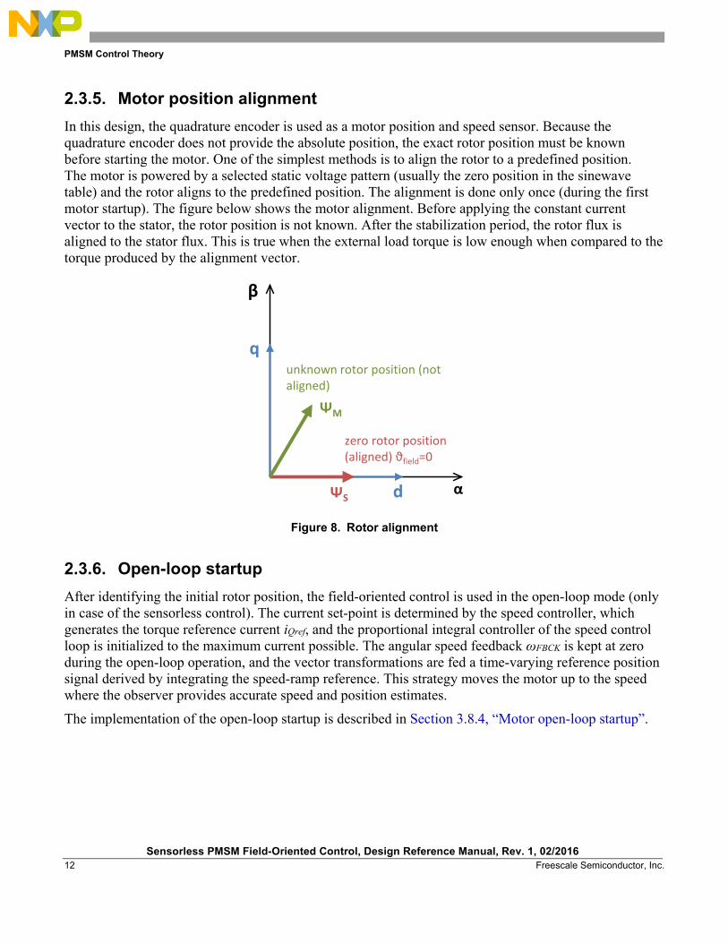
2.3.5. Motor position alignment In this design, the quadrature encoder is used as a motor position and speed sensor. Because the quadrature encoder does not provide the absolute position, the exact rotor position must be known before starting the motor. One of the simplest methods is to align the rotor to a predefined position. The motor is powered by a selected static voltage pattern (usually the zero position in the sinewave table) and the rotor aligns to the predefined position. The alignment is done only once (during the first motor startup). The figure below shows the motor alignment. Before applying the constant current vector to the stator, the rotor position is not known. After the stabilization period, the rotor flux is aligned to the stator flux. This is true when the external load torque is low enough when compared to the torque produced by the alignment vector.

Figure 8. Rotor alignment

2.3.6. Open-loop startup After identifying the initial rotor position, the field-oriented control is used in the open-loop mode (only in case of the sensorless control). The current set-point is determined by the speed controller, which generates the torque reference current iQref, and the proportional integral controller of the speed control loop is initialized to the maximum current possible. The angular speed feedback ωFBCK is kept at zero during the open-loop operation, and the vector transformations are fed a time-varying reference position signal derived by integrating the speed-ramp reference. This strategy moves the motor up to the speed where the observer provides accurate speed and position estimates.

The implementation of the open-loop startup is described in Section 3.8.4, “Motor open-loop startup”.

d α

β

qunknown rotor position (not aligned)

zero rotor position (aligned) ϑfield=0

ΨM

ΨS

PMSM Control Theory


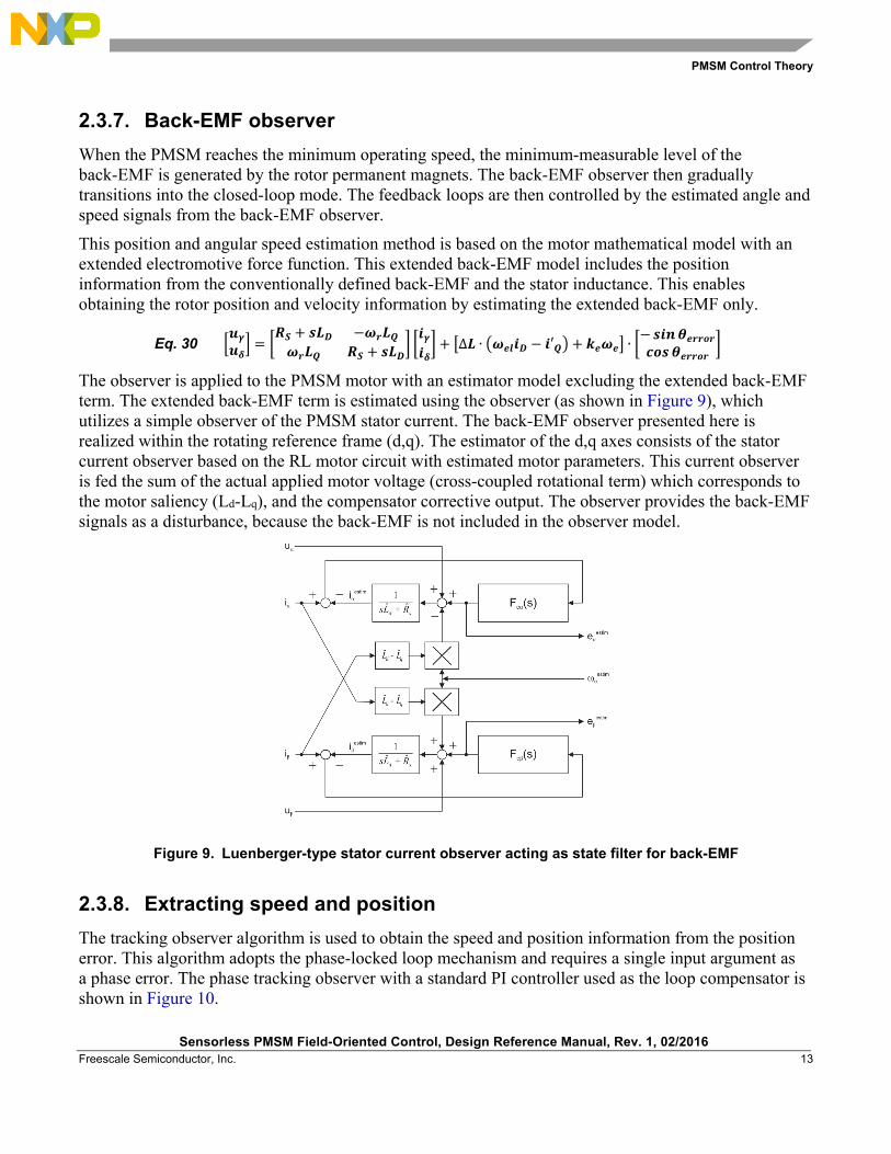
2.3.7. Back-EMF observer When the PMSM reaches the minimum operating speed, the minimum-measurable level of the back-EMF is generated by the rotor permanent magnets. The back-EMF observer then gradually transitions into the closed-loop mode. The feedback loops are then controlled by the estimated angle and speed signals from the back-EMF observer.

This position and angular speed estimation method is based on the motor mathematical model with an extended electromotive force function. This extended back-EMF model includes the position information from the conventionally defined back-EMF and the stator inductance. This enables obtaining the rotor position and velocity information by estimating the extended back-EMF only.

Eq. 30 �𝒖𝒖𝜸𝜸𝒖𝒖𝜹𝜹� = �

𝑹𝑹𝑺𝑺 + 𝒔𝒔𝑳𝑳𝑫𝑫 −𝒅𝒅𝒓𝒓𝑳𝑳𝑸𝑸𝒅𝒅𝒓𝒓𝑳𝑳𝑸𝑸 𝑹𝑹𝑺𝑺 + 𝒔𝒔𝑳𝑳𝑫𝑫

� �𝒊𝒊𝜸𝜸𝒊𝒊𝜹𝜹� + �∆𝑳𝑳 ∙ �𝒅𝒅𝒆𝒆𝒆𝒆𝒊𝒊𝑫𝑫 − 𝒊𝒊′𝑸𝑸� + 𝒌𝒌𝒆𝒆𝒅𝒅𝒆𝒆� ∙ �

− 𝒔𝒔𝒊𝒊𝒔𝒔𝜽𝜽𝒆𝒆𝒓𝒓𝒓𝒓𝒄𝒄𝒓𝒓𝒔𝒔𝒄𝒄𝒔𝒔𝜽𝜽𝒆𝒆𝒓𝒓𝒓𝒓𝒄𝒄𝒓𝒓

�

The observer is applied to the PMSM motor with an estimator model excluding the extended back-EMF term. The extended back-EMF term is estimated using the observer (as shown in Figure 9), which utilizes a simple observer of the PMSM stator current. The back-EMF observer presented here is realized within the rotating reference frame (d,q). The estimator of the d,q axes consists of the stator current observer based on the RL motor circuit with estimated motor parameters. This current observer is fed the sum of the actual applied motor voltage (cross-coupled rotational term) which corresponds to the motor saliency (Ld-Lq), and the compensator corrective output. The observer provides the back-EMF signals as a disturbance, because the back-EMF is not included in the observer model.

Figure 9. Luenberger-type stator current observer acting as state filter for back-EMF

2.3.8. Extracting speed and position The tracking observer algorithm is used to obtain the speed and position information from the position error. This algorithm adopts the phase-locked loop mechanism and requires a single input argument as a phase error. The phase tracking observer with a standard PI controller used as the loop compensator is shown in Figure 10.

Software Design


Figure 10. Block diagram of proposed PLL scheme for position estimation

3. Software Design This application is written as a simple C project with the inclusion of Embedded Software Libraries (FSLESL). Download these libraries from www.nxp.com/fslesl. They contain the necessary algorithms, math functions, observers, filters, and other features used in the application.

This section describes the software design of the sensorless PMSM FOC application. It describes the numerical scaling in the fixed-point fractional arithmetic of the controller first. Then it describes specific issues, such as speed and current sensing. In the end, it describes the control software implementation.

3.1. Data types This application uses several data types: (un)signed integer, fractional, and accumulator. The integer data types are useful for general-purpose computation; they are familiar to the MPU and MCU programmers. The fractional data types enable implementing numeric and digital signal processing algorithms. The accumulator data type is a combination of both; that means it has the integer and fractional portions.

This list shows the integer types defined in the libraries: • Unsigned 16-bit integer—<0 ; 65535> with a minimum resolution of 1 • Signed 16-bit integer—<-32768 ; 32767> with a minimum resolution of 1 • Unsigned 32-bit integer—<0 ; 4294967295> with a minimum resolution of 1 • Signed 32-bit integer—<-2147483648 ; 2147483647> with a minimum resolution of 1

This list shows the fractional types defined in the libraries: • Fixed-point 16-bit fractional—<-1 ; 1–2-15> with a minimum resolution of 2-15 • Fixed-point 32-bit fractional—<-1 ; 1–2-31> with a minimum resolution of 2-31

This list shows the accumulator types defined in the libraries: • Fixed-point 16-bit accumulator—<-256.0 ; 256.0–2-7> with a minimum resolution of 2-7 • Fixed-point 32-bit accumulator—<-65536.0 ; 65536.0–2-15> with a minimum resolution of 2-15

Software Design


3.2. Scaling of analog quantities This equation shows the relationship between the real and fractional representations:

Eq. 31 𝒇𝒇𝒓𝒓𝒔𝒔𝒔𝒔𝒅𝒅𝒊𝒊𝒄𝒄𝒔𝒔𝒔𝒔𝒆𝒆 𝒗𝒗𝒔𝒔𝒆𝒆𝒖𝒖𝒆𝒆 = 𝑹𝑹𝒆𝒆𝒔𝒔𝒆𝒆 𝒗𝒗𝒔𝒔𝒆𝒆𝒖𝒖𝒆𝒆𝑹𝑹𝒆𝒆𝒔𝒔𝒆𝒆 𝑺𝑺𝒖𝒖𝒔𝒔𝒔𝒔𝒅𝒅𝒊𝒊𝒅𝒅𝒔𝒔 𝒓𝒓𝒔𝒔𝒔𝒔𝒔𝒔𝒆𝒆

where: • Fractional Value—fractional representation of quantities [–] • Real Value—real quantity in physical units [..] • Real Quantity Range—maximum defined quantity value used for scaling in physical units [..]

Some examples of the quantities’ scaling are provided in the following subsections.

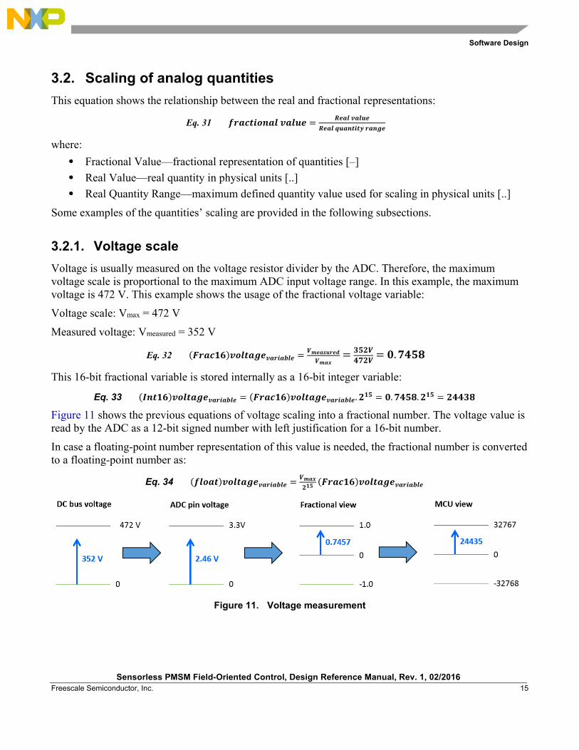
3.2.1. Voltage scale Voltage is usually measured on the voltage resistor divider by the ADC. Therefore, the maximum voltage scale is proportional to the maximum ADC input voltage range. In this example, the maximum voltage is 472 V. This example shows the usage of the fractional voltage variable: Voltage scale: Vmax = 472 V

Measured voltage: Vmeasured = 352 V

Eq. 32 (𝑭𝑭𝒓𝒓𝒔𝒔𝒔𝒔𝟏𝟏𝟔𝟔)𝒗𝒗𝒄𝒄𝒆𝒆𝒅𝒅𝒔𝒔𝒔𝒔𝒆𝒆𝒗𝒗𝒔𝒔𝒓𝒓𝒊𝒊𝒔𝒔𝒔𝒔𝒆𝒆𝒆𝒆 = 𝑽𝑽𝒎𝒎𝒆𝒆𝒔𝒔𝒔𝒔𝒖𝒖𝒓𝒓𝒆𝒆𝒅𝒅𝑽𝑽𝒎𝒎𝒔𝒔𝒔𝒔

= 𝟑𝟑𝟑𝟑𝟐𝟐𝑽𝑽𝟒𝟒𝟒𝟒𝟐𝟐𝑽𝑽 = 𝟎𝟎.𝟒𝟒𝟒𝟒𝟑𝟑𝟕𝟕

This 16-bit fractional variable is stored internally as a 16-bit integer variable:

Eq. 33 (𝑰𝑰𝒔𝒔𝒅𝒅𝟏𝟏𝟔𝟔)𝒗𝒗𝒄𝒄𝒆𝒆𝒅𝒅𝒔𝒔𝒔𝒔𝒆𝒆𝒗𝒗𝒔𝒔𝒓𝒓𝒊𝒊𝒔𝒔𝒔𝒔𝒆𝒆𝒆𝒆 = (𝑭𝑭𝒓𝒓𝒔𝒔𝒔𝒔𝟏𝟏𝟔𝟔)𝒗𝒗𝒄𝒄𝒆𝒆𝒅𝒅𝒔𝒔𝒔𝒔𝒆𝒆𝒗𝒗𝒔𝒔𝒓𝒓𝒊𝒊𝒔𝒔𝒔𝒔𝒆𝒆𝒆𝒆.𝟐𝟐𝟏𝟏𝟑𝟑 = 𝟎𝟎.𝟒𝟒𝟒𝟒𝟑𝟑𝟕𝟕.𝟐𝟐𝟏𝟏𝟑𝟑 = 𝟐𝟐𝟒𝟒𝟒𝟒𝟑𝟑𝟕𝟕

Figure 11 shows the previous equations of voltage scaling into a fractional number. The voltage value is read by the ADC as a 12-bit signed number with left justification for a 16-bit number.

In case a floating-point number representation of this value is needed, the fractional number is converted to a floating-point number as:

Eq. 34 (𝒇𝒇𝒆𝒆𝒄𝒄𝒔𝒔𝒅𝒅)𝒗𝒗𝒄𝒄𝒆𝒆𝒅𝒅𝒔𝒔𝒔𝒔𝒆𝒆𝒗𝒗𝒔𝒔𝒓𝒓𝒊𝒊𝒔𝒔𝒔𝒔𝒆𝒆𝒆𝒆 = 𝑽𝑽𝒎𝒎𝒔𝒔𝒔𝒔𝟐𝟐𝟏𝟏𝟑𝟑

(𝑭𝑭𝒓𝒓𝒔𝒔𝒔𝒔𝟏𝟏𝟔𝟔)𝒗𝒗𝒄𝒄𝒆𝒆𝒅𝒅𝒔𝒔𝒔𝒔𝒆𝒆𝒗𝒗𝒔𝒔𝒓𝒓𝒊𝒊𝒔𝒔𝒔𝒔𝒆𝒆𝒆𝒆

Figure 11. Voltage measurement

Software Design


3.2.2. Current scale Current is usually measured as a voltage drop on the shunt resistors, which is amplified by an operational amplifier. If both the positive and negative currents are needed, the amplified signal has an offset. The offset is generally half of the ADC range. The maximum current scale is then proportional to a half of the maximum ADC input voltage range (see Figure 12). Manipulation with the current variable is similar to manipulation with the voltage variable.

Figure 12. Current measurement

3.2.3. Angle scale The angles (such as rotor position) are represented as fixed-point 32-bit accumulators, where the lower 16-bits are in the range <-1 , 1), which corresponds to an angle in the range <-π , π). In a 16-bit signed integer value, the angle is represented as:

Eq. 35 −𝝅𝝅 = 𝟎𝟎𝒔𝒔𝟕𝟕𝟎𝟎𝟎𝟎𝟎𝟎

Eq. 36 𝝅𝝅 = 𝟎𝟎𝒔𝒔𝟒𝟒𝑭𝑭𝑭𝑭𝑭𝑭

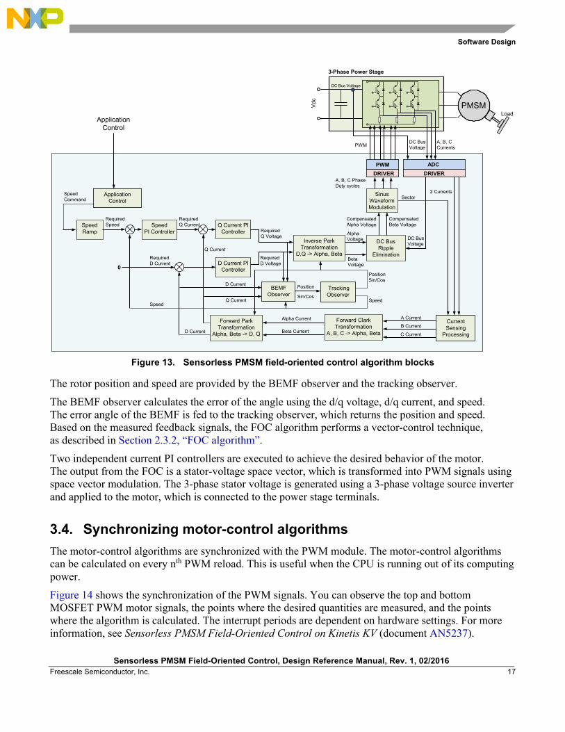
3.3. Application overview Figure 13 shows the FOC algorithm blocks of a PMSM. The state of the ON/OFF switch variable of the motor-control application part is scanned periodically. The speed command that is entered from the high-level application layer is processed by the means of a speed-ramp algorithm. The comparison between the actual speed command (obtained from the ramp algorithm output) and the measured speed generates a speed error. The speed error is input to the speed PI controller, generating a new desired level of reference for the torque-producing component of the stator current.

The DC-bus voltage and phase currents are sampled by the ADC. The ADC sampling is started by the PWM module trigger signals. A digital filter is applied to the sampled values of the DC-bus voltage. The phase currents are used unfiltered. The 3-phase motor current is reconstructed from two samples taken from the inverter’s shunt resistors. The reconstructed 3-phase current is then transformed into the space vectors and used by the FOC algorithm.

Software Design


Figure 13. Sensorless PMSM field-oriented control algorithm blocks

The rotor position and speed are provided by the BEMF observer and the tracking observer.

The BEMF observer calculates the error of the angle using the d/q voltage, d/q current, and speed. The error angle of the BEMF is fed to the tracking observer, which returns the position and speed. Based on the measured feedback signals, the FOC algorithm performs a vector-control technique, as described in Section 2.3.2, “FOC algorithm”.

Two independent current PI controllers are executed to achieve the desired behavior of the motor. The output from the FOC is a stator-voltage space vector, which is transformed into PWM signals using space vector modulation. The 3-phase stator voltage is generated using a 3-phase voltage source inverter and applied to the motor, which is connected to the power stage terminals.

3.4. Synchronizing motor-control algorithms The motor-control algorithms are synchronized with the PWM module. The motor-control algorithms can be calculated on every nth PWM reload. This is useful when the CPU is running out of its computing power.

Figure 14 shows the synchronization of the PWM signals. You can observe the top and bottom MOSFET PWM motor signals, the points where the desired quantities are measured, and the points where the algorithm is calculated. The interrupt periods are dependent on hardware settings. For more information, see Sensorless PMSM Field-Oriented Control on Kinetis KV (document AN5237).

DRIVER

3-Phase Power Stage

PWM

Forward Clark Transformation

A, B, C -> Alpha, Beta

Q Current PI Controller

ADCPWM

D Current PI Controller

DC Bus Ripple

Elimination

Application Control

A Current

AlphaVoltage

Beta Voltage

B Current

C Current

Alpha Current

Beta CurrentD Current

Required Q Voltage

RequiredD Voltage

CompensatedAlpha Voltage

Required Speed

DRIVER

6PMSM6PMSM

DC Bus Voltage

Sector

Load

DC Bus Voltage

PositionSin/Cos

Speed

RequiredQ Current

RequiredD Current

DC Bus Voltage

CompensatedBeta Voltage

A, B, C PhaseDuty cycles

2 CurrentsSinus Waveform Modulation

Current Sensing

Processing

A, B, C Currents

SpeedPI Controller

Tracking Observer

Position

Sin/Cos

Forward Park Transformation

Alpha, Beta -> D, Q

Speed

Application Control

Vdc

SpeedRamp

Q Current

D Current

Q Current

BEMF Observer

SpeedCommand

0

Inverse Park Transformation

D,Q -> Alpha, Beta

http://www.fsls.co/doc/AN5237

Software Design


Figure 14. Application timing

3.5. Calling algorithms This application is interrupt-driven, running in real time. There is one (or more) periodic-interrupt service routine executing the major application-control tasks.

The motor-control fast-loop algorithms are executed periodically in the ADC conversion complete interrupt. This interrupt has the highest priority level. When the interrupt is entered, the DC-bus voltage and motor phase currents are read and the PMSM FOC algorithm is calculated.

Figure 15. Fast-loop ISR

The slow-loop interrupt service routine is executed periodically when the independent FlexTimer reloads. It is basically a speed control.

Top PWM

Bottom PWM

Trigger

ADC conversion

Fast loop controlinterrupt

RELOAD

Fast loop controlPWM update

Trigger

RELOAD

Conversion complete

Software Design


Figure 16. Slow-loop ISR

The background loop is executed in the main application. It handles non-critical timing tasks, such as the communication with FreeMASTER over UART. The interrupt service routine calls the state machine function. The state machine function depends on the particular state. When in a dependent state, the particular state machine function is called, and it ensures that the correct state-machine logic and control algorithm is called. The state machine is described in the following sections.

3.6. Main state machine The state-machine structure is unified for all application components and it consists of four main states (see Figure 17). The states are:

• Fault—the system detected a fault condition and waits for the condition to be cleared. • Init—variables’ initialization. • Stop—the system is initialized and waiting for the Run command. • Run—the system is running and can be stopped by the Stop command.

There are transition functions between these state functions: • Init > Stop—initialization was done, the system is entering the Stop state. • Stop > Run—the Run command was applied, the system is entering the Run state if the Run

command was acknowledged. • Run > Stop—the Stop command was applied, the system is entering the Stop state if the Stop

command was acknowledged. • Fault > Stop—fault flag was cleared, the system is entering the Stop state. • Init, Stop, Run > Fault—a fault condition occurred, the system is entering the Fault state.

The state machine structure uses these flags to switch between the states: • SM_CTRL_INIT_DONE—if this flag is set, the system goes from the Init state to the Stop state. • SM_CTRL_FAULT—if this flag is set, the system goes from any state to the Fault state. • SM_CTRL_FAULT_CLEAR—if this flag is set, the system goes from the Fault state to the Init

state.

Software Design


• SM_CTRL_START—this flag informs the system that there is a command to go from the Stop state to the Run state. The transition function is called; nevertheless, the action must be acknowledged. The reason is that sometimes it can take time before the system is ready to be switched on.

• SM_CTRL_RUN_ACK—this flag acknowledges that the system can proceed from the Stop state to the Run state.

• SM_CTRL_STOP—this flag informs the system that there is a command to go from the Run state to the Stop state. The transition function is called; nevertheless, the action must be acknowledged. The reason is that the system must be switched off properly, which takes time.

• SM_CTRL_STOP_ACK—this flag acknowledges that the system can proceed from the Run state to the Stop state.

Figure 17. Main state machine diagram

The implementation of this state machine structure is done in the state_machine.c and state_machine.h files. The following code lines define the state machine structure: /* State machine control structure */ typedef struct { SM_APP_STATE_FCN_T const* psState; /* State functions */ SM_APP_TRANS_FCN_T const* psTrans; /* Transition functions */ SM_APP_CTRL uiCtrl; /* Control flags */ SM_APP_STATE_T eState; /* State */ } SM_APP_CTRL_T;

INIT

FAULT

RUN

STOP

RESET

SM_CTRL_INIT_DONESM_CTRL_FAULT

SM_CTRL_FAULT

SM_CTRL_START

SM_CTRL_STOP

SM_CTRL_FAULT_CLEAR

TransitionInit -> Stop

TransitionStop -> Run

SM_CTRL_RUN_ACK

TransitionRun -> Stop

SM_CTRL_STOP_ACK

TransitionRun -> Fault

SM_CTRL_FAULT

TransitionStop -> Fault

TransitionInit -> Fault

TransitionFault -> Stop

Software Design


The four variables used in the code are: • psState—pointer to the user state machine functions. The particular state machine function from

this table is called when the state machine is in a specific state. • psTrans—pointer to the user transient functions. The particular transient function is called when

the system goes from one state to another. • uiCtrl—controls the state machine behavior using the above-mentioned flags. • eState—this variable determines the actual state of the state machine.

The user state machine functions are defined in this structure: /* User state machine functions structure */ typedef struct { PFCN_VOID_VOID Fault; PFCN_VOID_VOID Init; PFCN_VOID_VOID Stop; PFCN_VOID_VOID Run; } SM_APP_STATE_FCN_T;

The user transient state machine functions are defined in this structure: /* User state-transition functions structure*/ typedef struct { PFCN_VOID_VOID FaultInit; PFCN_VOID_VOID InitFault; PFCN_VOID_VOID InitStop; PFCN_VOID_VOID StopFault; PFCN_VOID_VOID StopRun; PFCN_VOID_VOID RunFault; PFCN_VOID_VOID RunStop; } SM_APP_TRANS_FCN_T;

The control flag variable has these definitions: typedef unsigned short SM_APP_CTRL; /* State machine control command flags */ #define SM_CTRL_NONE 0x0 #define SM_CTRL_FAULT 0x1 #define SM_CTRL_FAULT_CLEAR 0x2 #define SM_CTRL_INIT_DONE 0x4 #define SM_CTRL_STOP 0x8 #define SM_CTRL_START 0x10 #define SM_CTRL_STOP_ACK 0x20 #define SM_CTRL_RUN_ACK 0x40

The state-identification variable has these definitions: /* Application state identification enum */ typedef enum { FAULT = 0, INIT = 1, STOP = 2, RUN = 3, } SM_APP_STATE_T;

Software Design


Call the state machine from the code periodically using the following inline function. This function’s input is the pointer to the state machine structure described above. This structure is declared and initialized in the code where the state machine is called: /* State machine function */ static inline void SM_StateMachineFast(SM_APP_CTRL_T *sAppCtrl) { gSM_STATE_TABLE_FAST[sAppCtrl -> eState](sAppCtrl); }

An example of initializing and using the state machine structure is described in the following section.

3.7. Motor state machine The motor state machines are based on the main state machine structure. The Run state sub-states are added on top of the main structure to control the motors properly. This is the description of the main states’ user functions:

• Fault—the system faces a fault condition and waits until the fault flags are cleared. The DC-bus voltage is measured and filtered.

• Init—variables’ initialization. • Stop—the system is initialized and waiting for the Run command. The PWM output is disabled.

The DC-bus voltage is measured and filtered. • Run—the system is running and can be stopped by the Stop command. The Run sub-state

functions are called from here.

There are transition functions between these state functions: • Init > Stop—nothing is processed in this function. • Stop > Run:

— The duty cycle is initialized to 50 %. — The PWM output is enabled. — The current ADC channels are initialized. — The Calib sub-state is set as the initial Run sub-state.

• Run > Stop: — The Stop command was applied and the system enters the Stop state if the Stop command

was acknowledged. • Fault > Stop

— All state variables and accumulators are initialized. • Init, Stop > Fault

— The PWM output is disabled. • Run > Fault:

— Certain current and voltage variables are zeroed. — The PWM output is disabled.

Software Design


The Run sub-states are called when the state machine is in the Run state. The Run sub-state functions are:

• Calib: — The current channels’ ADC offset calibration. — The DC-bus voltage is measured and filtered. — The PWM is set to 50 % and its output is enabled. — The current channel offsets are measured and filtered. — After the calibration time expires, the system is switched to Ready.

• Ready: — The PWM is set to 50 % and its output is enabled. — The current is measured and the ADC channels are set up. — The DC-bus voltage is measured. — Certain variables are initialized.

• Align: — The current is measured and the ADC channels are set up. — The DC-bus voltage is measured and filtered. — The rotor-alignment algorithm is called and the PWM is updated. — After the alignment time expires, the system is switched to Startup.

• Startup: — The current is measured and the ADC channels are set up. — The BEMF observer algorithm is called to estimate the speed and position. — The FOC algorithm is called and the PWM is updated. — The DC-bus voltage is measured and filtered. — The open-loop start-up algorithm is called. — The estimated speed is filtered (in case the filter is necessary). — If the startup is successful, the system is switched to the Spin state; otherwise, it is

switched to the Freewheel state. • Spin:

— The current is measured and the ADC channels are set up. — The BEMF observer algorithm is called to estimate the speed and position. — The FOC algorithm is called and the PWM is updated. — The motor starts spinning. — The DC-bus voltage is measured and filtered. — The estimated speed is filtered (in case the filter is necessary). — The speed ramp and the speed PI controller algorithms are called.

Software Design


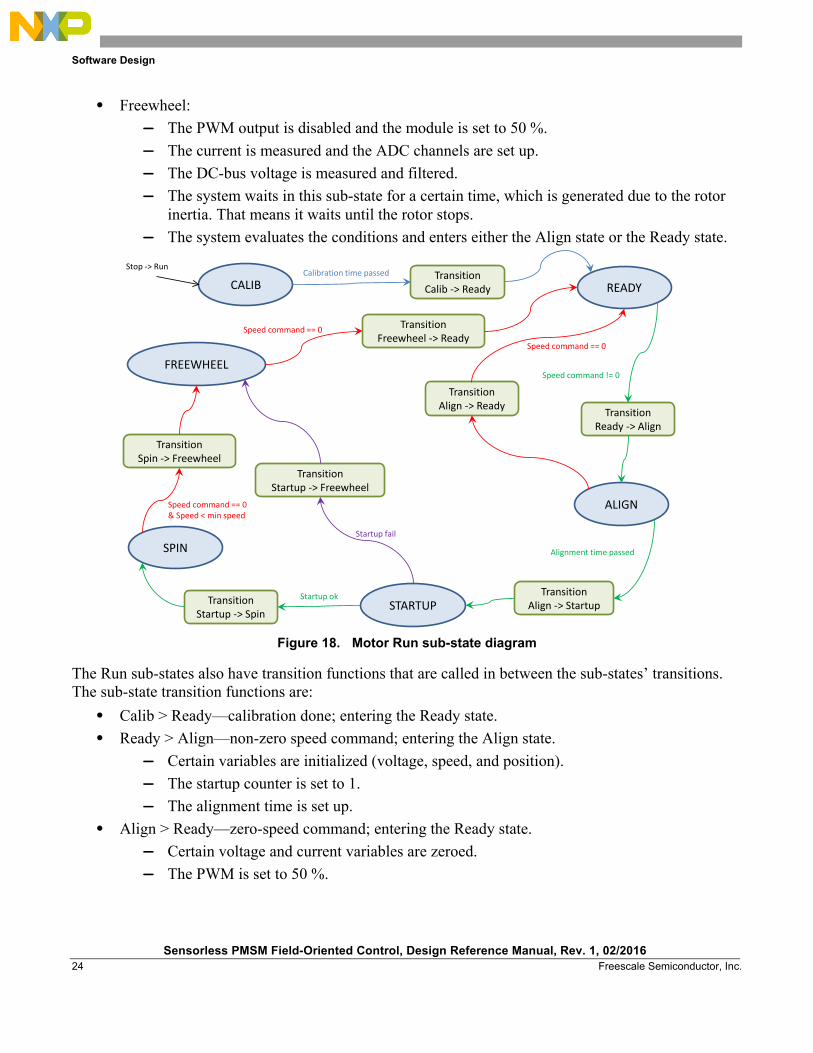
• Freewheel: — The PWM output is disabled and the module is set to 50 %. — The current is measured and the ADC channels are set up. — The DC-bus voltage is measured and filtered. — The system waits in this sub-state for a certain time, which is generated due to the rotor

inertia. That means it waits until the rotor stops. — The system evaluates the conditions and enters either the Align state or the Ready state.

Figure 18. Motor Run sub-state diagram

The Run sub-states also have transition functions that are called in between the sub-states’ transitions. The sub-state transition functions are:

• Calib > Ready—calibration done; entering the Ready state. • Ready > Align—non-zero speed command; entering the Align state.

— Certain variables are initialized (voltage, speed, and position). — The startup counter is set to 1. — The alignment time is set up.

• Align > Ready—zero-speed command; entering the Ready state. — Certain voltage and current variables are zeroed. — The PWM is set to 50 %.

CALIB READY

ALIGN

FREEWHEEL

SPIN

TransitionCalib -> Ready

TransitionReady -> Align

TransitionAlign -> StartupTransition

Startup -> SpinSTARTUP

TransitionStartup -> Freewheel

TransitionSpin -> Freewheel

TransitionFreewheel -> Ready

Stop -> Run

Speed command != 0

Alignment time passed

Startup ok

Speed command == 0& Speed < min speed

Speed command == 0

Startup fail

TransitionAlign -> Ready

Calibration time passed

Speed command == 0

Software Design


• Align > Startup—alignment is done; entering the Startup state. — The filters and control variables are initialized. — The PWM is set to 50 %.

• Startup > Spin—startup is successful; entering the Spin state. • Startup > Freewheel.

— Certain variables are initialized (voltage, speed, and position). — The startup counter is set to 1. — The Freewheel time is set up.

• Spin > Freewheel— zero speed command; entering the Freewheel state. — Certain variables are initialized (voltage, speed, and position). — The startup counter is set to 1. — The Freewheel time is set up.

• Freewheel > Ready—freewheel time elapsed; entering the Ready state. — The PWM output is enabled.

The implementation of this motor state-machine structure is done in the M1_statemachine.c and M1_statemachine.h files. Each state is doubled. States with the Fast suffix are called in the fast loop and states with the Slow suffix are called in the slow loop. However, the state transitions are not doubled and the state machine flow is controlled from the fast-loop state machine only. Here is the description of the main state-machine structure:

• The main states’ user function prototypes are: static void M1_StateFault(void); static void M1_StateInit(void); static void M1_StateStop(void); static void M1_StateRun(void);

• The main states’ user transient function prototypes are: static void M1_TransFaultStop(void); static void M1_TransInitFault(void); static void M1_TransInitStop(void); static void M1_TransStopFault(void); static void M1_TransStopRun(void); static void M1_TransRunFault(void); static void M1_TransRunStop(void);

• The main states functions table initialization is: /* State machine functions field */ static const SM_APP_STATE_FCN_T msSTATE = {M1_StateFault, M1_StateInit, M1_StateStop, M1_StateRun};

• The main state transient functions table initialization is: /* State-transition functions field */ static const SM_APP_TRANS_FCN_T msTRANS = {M1_TransFaultStop, M1_TransInitFault, M1_TransInitStop, M1_TransStopFault, M1_TransStopRun, M1_TransRunFault, M1_TransRunStop};

Software Design


• Finally, the main state machine structure initialization is: /* State machine structure declaration and initialization */ SM_APP_CTRL_T gsM1_Ctrl = { /* gsM1_Ctrl.psState, User state functions */ &msSTATE, /* gsM1_Ctrl.psTrans, User state-transition functions */ &msTRANS, /* gsM1_Ctrl.uiCtrl, Default no control command */ SM_CTRL_NONE, /* gsM1_Ctrl.eState, Default state after reset */ INIT };

• Similarly, the Run sub-state machine is declared. Thus, the Run sub-state identification variable has these definitions:

typedef enum { M1_CALIB = 0, M1_READY = 1, M1_ALIGN = 2, M1_STARTUP = 3, M1_SPIN = 4, M1_FREEWHEEL = 5 } M1_RUN_SUBSTATE_T; /* Run sub-states */

• For the Run sub-states, two sets of user functions are defined. The user function prototypes of the Run sub-states are:

static void M1_StateRunCalib(void); static void M1_StateRunReady(void); static void M1_StateRunAlign(void); static void M1_StateRunStartup(void); static void M1_StateRunSpin(void); static void M1_StateRunFreewheel(void);

• The Run sub-states’ user transient function prototypes are: static void M1_TransRunCalibReady(void); static void M1_TransRunReadyAlign(void); static void M1_TransRunAlignStartup(void); static void M1_TransRunAlignReady(void); static void M1_TransRunStartupSpin(void); static void M1_TransRunStartupFreewheel(void); static void M1_TransRunSpinFreewheel(void); static void M1_TransRunFreewheelReady(void);

• The Run sub-states functions table initialization is: /* Sub-state machine functions field */ static const PFCN_VOID_VOID mM1_STATE_RUN_TABLE[6] = { M1_StateRunCalib, M1_StateRunReady, M1_StateRunAlign, M1_StateRunStartup, M1_StateRunSpin, M1_StateRunFreewheel };

Software Design


• The state machine is called from the interrupt service routine, as mentioned in Section 3.5, “Calling algorithms”. The code syntax used for calling the state machine is:

/* StateMachine call */ SM_StateMachine(&gsM1_Ctrl);

• Inside the user Run state function, the sub-state functions are called as: /* Run sub-state function */ mM1_STATE_RUN_TABLE[meM1_StateRun]();

where the variable identifies the Run sub-state.

3.8. Sensorless PMSM control The application controls the PMSM in the sensorless mode. It is possible to control more PMSMs using one controller (if the MCU enables it). To avoid the multiplicity of routines in the memory, the application uses a set of routines where the inputs are the structures of the particular motors. This approach saves the necessary program flash memory in the application.

It is necessary to understand the fast-loop control loop implementation as a whole, and then break it down to pieces.

Figure 19. Fast-loop control flowchart

Figure 13 shows that the application requires sensors and estimators (current, DC-bus voltage, estimated speed, etc.) and actuators (PWM, etc.) to observe and control the whole system. The sensors and actuators are encapsulated into the dedicated modules within the unified interface called MCDRV. For more information on MCDRV, see Sensorless PMSM Field-Oriented Control on Kinetis KV (document AN5237).

http://www.fsls.co/doc/AN5237

Software Design


3.8.1. MCS—field-oriented control There is a single function executing the current FOC or the voltage FOC. The current FOC means that the inputs to this function are the required D and Q currents, and these currents are controlled to the required values by varying the D and Q voltages applied to the motor. The voltage control mode means that the input to this function are the required D and Q voltages that are applied to the motor. Choose between the current/voltage control using the bCurrentLoopOn flag. Example 1 belongs to the code implementation.

This FOC mode is optimized into one function which has one input/output pointer to a structure. The prototype of the function is: void MCS_PMSMFocCtrlA1(MCS_PMSM_FOC_A1_T *psFocPMSM)

The structure referred to by the input/output structure pointer is defined in this example:

Example 1. Field-oriented current control code typedef struct { GFLIB_CTRL_PI_P_AW_T_A32 sIdPiParams; /* Id PI controller parameters */ GFLIB_CTRL_PI_P_AW_T_A32 sIqPiParams; /* Iq PI controller parameters */ GDFLIB_FILTER_IIR1_T_F32 sUDcBusFilter; /* Dc bus voltage filter */ GMCLIB_3COOR_T_F16 sIABC; /* Measured 3-phase current */ GMCLIB_2COOR_ALBE_T_F16 sIAlBe; /* Alpha/Beta current */ GMCLIB_2COOR_DQ_T_F16 sIDQ; /* DQ current */ GMCLIB_2COOR_DQ_T_F16 sIDQReq; /* DQ required current */ GMCLIB_2COOR_DQ_T_F16 sIDQError; /* DQ current error */ GMCLIB_3COOR_T_F16 sDutyABC; /* Applied duty cycles ABC */ GMCLIB_2COOR_ALBE_T_F16 sUAlBeReq; /* Required Alpha/Beta voltage */ GMCLIB_2COOR_ALBE_T_F16 sUAlBeComp; /* Compensated to DC bus Alpha/Beta voltage GMCLIB_2COOR_DQ_T_F16 sUDQReq; /* Required DQ voltage */ GMCLIB_2COOR_DQ_T_F16 sUDQEst; /* BEMF observer input DQ voltages */ GMCLIB_2COOR_SINCOS_T_F16 sAnglePosEl; /* Electrical position sin/cos (at the moment of PWM current reading) */ AMCLIB_BEMF_OBSRV_DQ_T_A32 sBemfObsrv; /* BEMF observer in DQ */ AMCLIB_TRACK_OBSRV_T_F32 sTo; /* Tracking observer */ GDFLIB_FILTER_IIR1_T_F32 sSpeedElEstFilt; /* Estimated speed filter */ frac16_t f16SpeedElEst; /* Rotor electrical speed estimated */ uint16_t ui16SectorSVM; /* SVM sector */ frac16_t f16PosEl; /* Electrical position */ frac16_t f16PosElExt; /* Electrical position set from external function - sensor, open loop */ frac16_t f16PosElEst; /* Rotor electrical position estimated*/ frac16_t f16DutyCycleLimit; /* Max. allowable duty cycle in frac */ frac16_t f16UDcBus; /* DC bus voltage */ frac16_t f16UDcBusFilt; /* Filtered DC bus voltage */ bool_t bCurrentLoopOn; /* Flag enabling calculation of current control loop */ bool_t bPosExtOn; /* Flag enabling use of electrical position passed from other functions */ bool_t bOpenLoop; /* Position estimation loop is open */ bool_t bIdPiStopInteg; /* Id PI controller manual stop integration bool_t bIqPiStopInteg; /* Iq PI controller manual stop integration } MCS_PMSM_FOC_A1_T;

Software Design


This structure contains all the necessary variables or sub-structures for the field-oriented control algorithm implementation. The types used in this structure are defined in the Embedded Software Libraries (FSLESL). Here is a description of the items used in this application:

• D and Q current PI controllers—serve to control the D and Q currents. • DC-bus voltage first-order IIR filter—serves to filter the DC-bus voltage. • A, B, and C currents—measured 3-phase current; input to the algorithm. • Alpha and beta currents—currents transformed into the alpha/beta frame. • D and Q currents—currents transformed into the D/Q frame. • Required D and Q currents—required currents in the D/Q frame; input to the algorithm. • D and Q current error—error (difference) between the required and the measured D/Q currents. • A, B, and C duty cycles—3-phase duty cycles; output from the algorithm. • Required alpha and beta voltages—required voltages in the alpha/beta frame. • Compensated required alpha and beta voltages—the previous item recalculated on the actual

level of the DC-bus voltage. • Required D and Q voltages—required voltages in the alpha/beta frame; outputs from the PI

controllers. • Sin/Cos angle—rotor estimated electrical angle (sine, cosine). • Duty cycle limit—this variable limits the maximum value of the A, B, and C duty cycles. • DC-bus voltage—measured DC-bus voltage. • Filtered DC-bus voltage—filtered value of the previous item. • SVM sector—sector information; output from the SVM algorithm. • D current saturation flag—saturation flag for the D-current PI controller. • Q current saturation flag—saturation flag for the Q-current PI controller. • Speed startup flag—indicates that the motor is in startup.

This routine calculates the field-oriented control. The inputs to this routine include the 3-phase current, DC-bus voltage, the electrical position, and the required D and Q currents. The output from this routine are the 3-phase duty cycle, SVM sector, and the saturation flags of the PI controllers. The PI controllers and filters have structures that must be initialized before using this routine.

This routine is called in the fast loop state machine and its process flow chart is shown in the below figure. This function uses algorithms from the Embedded Software Libraries (FSLESL); the functions’ names may differ from one platform to another.

Software Design


Figure 20. FOC flowchart

3.8.2. MCS—scalar control The scalar control (V/Hz) is another control function. It is recommended to run the application in this mode only while the application is mastered using MCAT tool, because this tool automatically calculates the voltage/frequency ratio based on the motor parameters. Similar to the previous algorithms, this control mode is optimized into one function which has two input/output pointers to a structure. The prototype of this function is: void MCS_PMSMScalarCtrlA1(MCS_PMSM_FOC_A1_T *psFocPMSM, MCS_SCALAR_A1_T *psScalarPMSM)

bPosExtOn

External position Estimated position

Angle (sin/cos) calculation

Use estimated or External position?

Park transformation

Clark transformation

Speed/position estimation

Speed filter

bOpenLoop

Park transformation

bCurrentLoopOn

Inverse Park transformation

DCbus ripple elimination

Space vector modulation

DQ current errors

D controller limit

D current control

Q controller limit

Q current control

A,B,C currents

Last PWM update electrical position

Alpha, Beta currents

D,Q current and voltage

New electrical position/speed

Return from FOC function

FOC function call

Recalculate D,Q currents from new electrical position

Current control enabled

D,Q voltage, electrical angle

Alpha, Beta voltage

Alpha, Beta voltage compensated

A,B,C duty cycles, SVM sector

Required D,Q currentMeasured D,Q current

DCbus voltage, max Duty cycle

D current error

𝐿𝑖𝑚𝑖𝑡 = 𝑈𝐷𝐶𝑏𝑢𝑠 � 𝑚𝑎𝑎𝑥 𝑑𝑢𝑡𝑦 𝑐𝑦𝑐𝑙𝑒𝑒

DCbus voltage, max Duty cycle, D controller voltage

𝐿𝑖𝑚𝑖𝑡 = 𝑈𝐷𝐶𝑏𝑢𝑠 � 𝑚𝑎𝑎𝑥 𝑑𝑢𝑡𝑦 𝑐𝑦𝑐𝑙𝑒𝑒 2 − 𝑈𝐷2

Q current error

Software Design


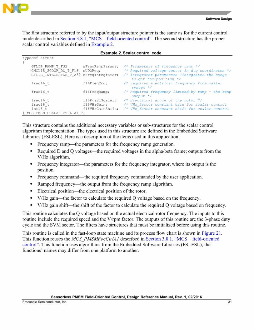
The first structure referred to by the input/output structure pointer is the same as for the current control mode described in Section 3.8.1, “MCS—field-oriented control”. The second structure has the proper scalar control variables defined in Example 2.

Example 2. Scalar control code typedef struct { GFLIB_RAMP_T_F32 sFreqRampParams; /* Parameters of frequency ramp */ GMCLIB_2COOR_DQ_T_F16 sUDQReq; /* Required voltage vector in d,q coordinates */ GFLIB_INTEGRATOR_T_A32 sFreqIntegrator; /* integrator parameters (integrates the omega to get the position */ frac16_t f16FreqCmd; /* required electrical frequency from master system */ frac16_t f16FreqRamp; /* Required frequency limited by ramp - the ramp output */ frac16_t f16PosElScalar; /* Electrical angle of the rotor */ frac16_t f16VHzGain; /* VHz_factor constant gain for scalar control int16_t f16VHzGainShift; /* VHz_factor constant shift for scalar control } MCS_PMSM_SCALAR_CTRL_A1_T;

This structure contains the additional necessary variables or sub-structures for the scalar control algorithm implementation. The types used in this structure are defined in the Embedded Software Libraries (FSLESL). Here is a description of the items used in this application:

• Frequency ramp—the parameters for the frequency ramp generation. • Required D and Q voltages—the required voltages in the alpha/beta frame; outputs from the

V/Hz algorithm. • Frequency integrator—the parameters for the frequency integrator, where its output is the

position. • Frequency command—the required frequency commanded by the user application. • Ramped frequency—the output from the frequency ramp algorithm. • Electrical position—the electrical position of the rotor. • V/Hz gain—the factor to calculate the required Q voltage based on the frequency. • V/Hz gain shift—the shift of the factor to calculate the required Q voltage based on frequency.

This routine calculates the Q voltage based on the actual electrical rotor frequency. The inputs to this routine include the required speed and the V/rpm factor. The outputs of this routine are the 3-phase duty cycle and the SVM sector. The filters have structures that must be initialized before using this routine.

This routine is called in the fast-loop state machine and its process flow chart is shown in Figure 21. This function reuses the MCS_PMSMFocCtrlA1 described in Section 3.8.1, “MCS—field-oriented control”. This function uses algorithms from the Embedded Software Libraries (FSLESL); the functions’ names may differ from one platform to another.

Software Design


Figure 21. Scalar control flowchart

3.8.3. Rotor alignment This application performs the rotor alignment before starting the motor. That means the rotor is forced to a known position.

Similarly to the previous algorithms, the alignment is optimized into one function which has one input/output pointer to a structure. The prototype of the function is: void MCS_PMSMAlignmentA1(MCS_PMSM_FOC_A1_T *psFocPMSM, MCS_ALIGNMENT_A1_T *psAlignment)

This function uses the FOC structure described in Section 3.8.1, “MCS—field-oriented control”. The alignment variables are contained in the alignment structure referred to by the second pointer. The alignment structure definition is:

Example 3. Alignment code typedef struct { frac16_t f16UdReq; /* Required D voltage at alignment */ uint16_t ui16Time; /* Alignment time duration */ uint16_t ui16TimeHalf; /* Alignment half time duration */ }MCS_ALIGNMENT_A1_T; /* PMSM simple two-step Ud voltage alignment */

The structure contains the variables necessary to perform the rotor alignment. The structure is described as follows:

• D voltage—the required voltage applied in the D axis during the alignment. • Alignment duration—the duration of the alignment. • Alignment halftime—the time for which the 120-degree position is required; when this time

passes, the 0-degree position is applied.

Frequency Ramp

Frequency integration

Volt/Hertz calculation

FOC control

Ramped frequency

Required D,Q voltage

Return from Scalar function

Scalar function call

Required D,Q voltage, Electrical position

A,B,C duty cycles, SVM sector

Required frequency

Software Design


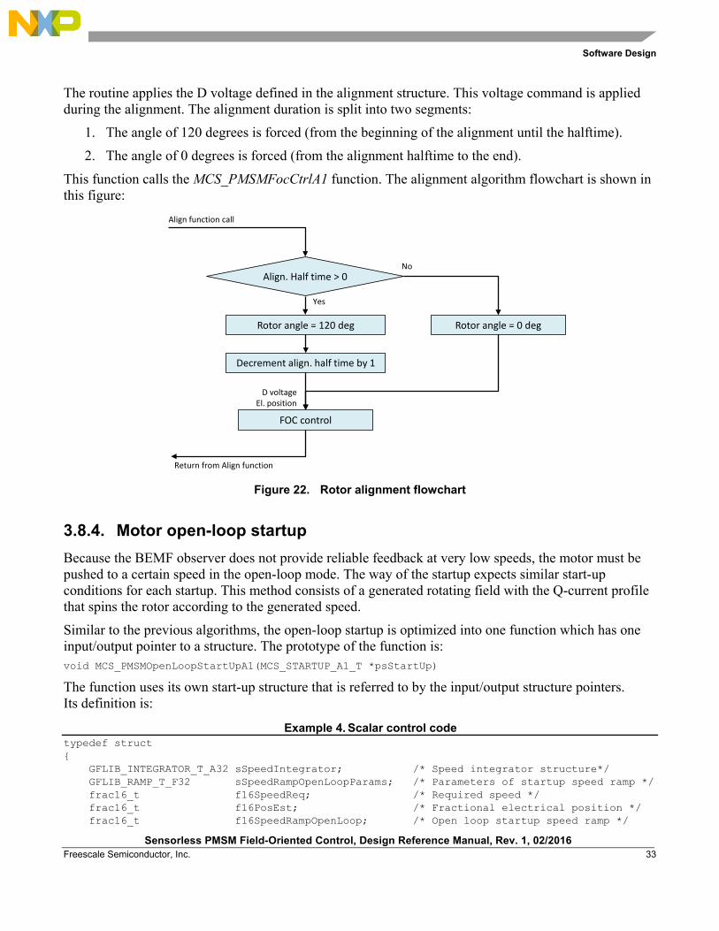
The routine applies the D voltage defined in the alignment structure. This voltage command is applied during the alignment. The alignment duration is split into two segments:

1. The angle of 120 degrees is forced (from the beginning of the alignment until the halftime).

2. The angle of 0 degrees is forced (from the alignment halftime to the end).

This function calls the MCS_PMSMFocCtrlA1 function. The alignment algorithm flowchart is shown in this figure:

Figure 22. Rotor alignment flowchart

3.8.4. Motor open-loop startup Because the BEMF observer does not provide reliable feedback at very low speeds, the motor must be pushed to a certain speed in the open-loop mode. The way of the startup expects similar start-up conditions for each startup. This method consists of a generated rotating field with the Q-current profile that spins the rotor according to the generated speed.

Similar to the previous algorithms, the open-loop startup is optimized into one function which has one input/output pointer to a structure. The prototype of the function is: void MCS_PMSMOpenLoopStartUpA1(MCS_STARTUP_A1_T *psStartUp)

The function uses its own start-up structure that is referred to by the input/output structure pointers. Its definition is:

Example 4. Scalar control code typedef struct { GFLIB_INTEGRATOR_T_A32 sSpeedIntegrator; /* Speed integrator structure*/ GFLIB_RAMP_T_F32 sSpeedRampOpenLoopParams; /* Parameters of startup speed ramp */ frac16_t f16SpeedReq; /* Required speed */ frac16_t f16PosEst; /* Fractional electrical position */ frac16_t f16SpeedRampOpenLoop; /* Open loop startup speed ramp */

Align. Half time > 0

Rotor angle = 0 deg

Return from Align function

Align function call

Rotor angle = 120 deg

Decrement align. half time by 1

FOC control

D voltageEl. position

No

Yes

Software Design


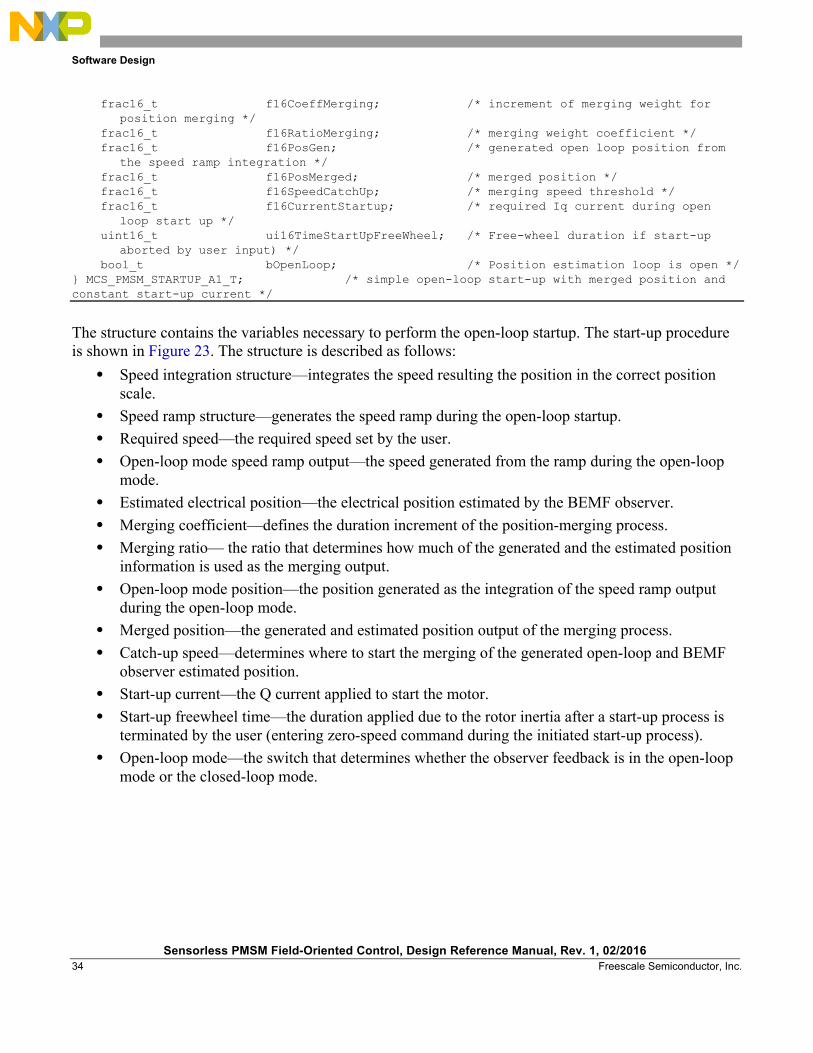
frac16_t f16CoeffMerging; /* increment of merging weight for position merging */ frac16_t f16RatioMerging; /* merging weight coefficient */ frac16_t f16PosGen; /* generated open loop position from the speed ramp integration */ frac16_t f16PosMerged; /* merged position */ frac16_t f16SpeedCatchUp; /* merging speed threshold */ frac16_t f16CurrentStartup; /* required Iq current during open loop start up */ uint16_t ui16TimeStartUpFreeWheel; /* Free-wheel duration if start-up aborted by user input) */ bool_t bOpenLoop; /* Position estimation loop is open */ } MCS_PMSM_STARTUP_A1_T; /* simple open-loop start-up with merged position and constant start-up current */

The structure contains the variables necessary to perform the open-loop startup. The start-up procedure is shown in Figure 23. The structure is described as follows:

• Speed integration structure—integrates the speed resulting the position in the correct position scale.

• Speed ramp structure—generates the speed ramp during the open-loop startup. • Required speed—the required speed set by the user. • Open-loop mode speed ramp output—the speed generated from the ramp during the open-loop

mode. • Estimated electrical position—the electrical position estimated by the BEMF observer. • Merging coefficient—defines the duration increment of the position-merging process. • Merging ratio— the ratio that determines how much of the generated and the estimated position

information is used as the merging output. • Open-loop mode position—the position generated as the integration of the speed ramp output

during the open-loop mode. • Merged position—the generated and estimated position output of the merging process. • Catch-up speed—determines where to start the merging of the generated open-loop and BEMF

observer estimated position. • Start-up current—the Q current applied to start the motor. • Start-up freewheel time—the duration applied due to the rotor inertia after a start-up process is

terminated by the user (entering zero-speed command during the initiated start-up process). • Open-loop mode—the switch that determines whether the observer feedback is in the open-loop

mode or the closed-loop mode.

Software Design


Figure 23. Motor open-loop startup

The start-up procedure is a complex process which is based on applying the torque and expecting the speed to respond accordingly. Therefore, the torque is proportional to the Q current which is kept constant.

The speed is ramped with the constant acceleration while the Q current is kept at the defined level. When the catch-up speed is reached, the merging ratio is incremented with the merging coefficient. This ratio determines how much of the estimated position information is merged with the generated (predicted) position information. At the beginning, it is 0 % for the estimated position information and 100 % for the predicted position information. Their sum is always 1.

After the system finishes merging the BEMF position, the loop is closed, and the motor is successfully started with the speed control turned on.

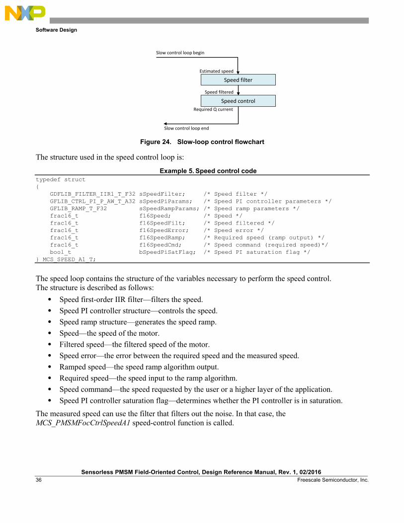
3.8.5. Speed loop The speed loop is calculated in the Run > Spin sub-state (in the M1_StateRunSpin function). The slow-loop frequency is divided to reach a lower frequency of control.

In this application, the slow-loop control is very simple. See the following figure.

Q current

Speed

Start-up current

Predicted (generated)

Estimated (observer)

100 %

Merge

Start-up commences

Reachedcatch-up speed

BEMF observer closed-loop

Speed control closed-loop

Observer on

Software Design


Figure 24. Slow-loop control flowchart

The structure used in the speed control loop is:

Example 5. Speed control code typedef struct { GDFLIB_FILTER_IIR1_T_F32 sSpeedFilter; /* Speed filter */ GFLIB_CTRL_PI_P_AW_T_A32 sSpeedPiParams; /* Speed PI controller parameters */ GFLIB_RAMP_T_F32 sSpeedRampParams; /* Speed ramp parameters */ frac16_t f16Speed; /* Speed */ frac16_t f16SpeedFilt; /* Speed filtered */ frac16_t f16SpeedError; /* Speed error */ frac16_t f16SpeedRamp; /* Required speed (ramp output) */ frac16_t f16SpeedCmd; /* Speed command (required speed)*/ bool_t bSpeedPiSatFlag; /* Speed PI saturation flag */ } MCS_SPEED_A1_T;

The speed loop contains the structure of the variables necessary to perform the speed control. The structure is described as follows:

• Speed first-order IIR filter—filters the speed. • Speed PI controller structure—controls the speed. • Speed ramp structure—generates the speed ramp. • Speed—the speed of the motor. • Filtered speed—the filtered speed of the motor. • Speed error—the error between the required speed and the measured speed. • Ramped speed—the speed ramp algorithm output. • Required speed—the speed input to the ramp algorithm. • Speed command—the speed requested by the user or a higher layer of the application. • Speed PI controller saturation flag—determines whether the PI controller is in saturation.

The measured speed can use the filter that filters out the noise. In that case, the MCS_PMSMFocCtrlSpeedA1 speed-control function is called.

Speed filter

Speed controlSpeed filtered

Required Q current

Slow control loop end

Slow control loop begin

Estimated speed

Software Design


This function performs these tasks (see Figure 25): • Generation of the saturation flag based on the Q current and speed PI controller saturation flag,

but only if the speed request is higher than the actual speed. • Speed ramp generation. This ramp has an input of the previously mentioned saturation flag.

That means the ramp is generated towards the requested speed; when the saturation flag is set, the ramp returns slowly (with a different increment) towards the actual speed to get the system out of saturation.

• Speed PI controller. This algorithm controls the speed. The input is the error (the difference) between the desired speed and the actual speed. Its output is the desired Q current.

Figure 25. Speed control flowchart

Saturation flag evaluation

Speed error

Speed ramp

Speed PI control

Required speed,Saturation flag

Ramped speed,Actual speed

Return from Speed control function

Speed control function call

Required D,Q voltage, Electrical position

Required Q current


4. Acronyms and Abbreviations This table lists the acronyms and abbreviations used in this document:

Table 2. Acronyms and abbreviations

Term Meaning AC Alternating current

ACIM AC Induction Motor

ADC Analogue-to-digital converter

FSLESL Freescale’s Embedded Software Libraries

BEMF Back-electromotive force

DC Direct current

DRM Design reference manual

FTM Flex Timer Module

ISR Interrupt Service Routine

MCAT Motor Control Application Tuning

MCDRV Motor Control Drivers

MCU Microcontroller Unit

PMSM Permanent Magnet Synchronous Motor

PWM Pulse-width modulation

SC Scalar Control

SVM Space Vector Modulation

VC Vector Control

XBAR Crossbar unit

List of Symbols


5. List of Symbols This table lists the symbols used in this document:

Table 3. List of symbols

Symbol Definition d,q Rotational orthogonal coordinate system

uγ, uδ Alpha/Beta BEMF observer error

isa, isb, isc Stator currents of the a, b, and c phases

isd,q, is(d,q) Stator currents in the d, q coordinate system

iγ,δ Stator currents in estimated d, q coordinate system

isα,β, is(α,β) Stator currents in α, β coordinate system

îsg Stator current space vector in general reference frame

isx, isy Stator current space vector components in general reference frame

îrg Rotor current space vector in general reference frame

irx, iry Rotor current space vector components in general reference frame

J Mechanical inertia

KM Motor constant

ke BEMF constant

Ls Stator-phase inductance

Lsd, LD Stator-phase inductance d axis

Lsq, LQ Stator-phase inductance q axis

p Number of poles per phase

Rs Stator-phase resistance

s Derivative operator

TL Load torque

uSα,β,uS(α,β) Stator voltages in α, β coordinate system

uSd,q, uS(d,q) Stator voltages in d, q coordinate system

ΨSα,β Stator magnetic fluxes in α, β coordinate system

ΨSd,q Stator magnetic fluxes in d, q coordinate system

ΨM Rotor magnetic flux

θr Rotor position angle in α, β coordinate system

ω, ωr, ωe Electrical rotor angular speed / fields angular speed

Revision History


6. Revision History This table summarizes the changes made to this document since the initial release.

Table 4. Revision history

Revision

number Date Substantive changes

0 04/2014 Initial release.

1 02/2016 Updated the document to correspond to the new software structure. Updated the state machine description. Added Section 4, “Acronyms and Abbreviations” and Section 5, “List of Symbols”.

Document Number: DRM148 Rev. 1

02/2016

How to Reach Us:

Home Page: freescale.com

Web Support: freescale.com/support

Information in this document is provided solely to enable system and software implementers to use Freescale products. There are no express or implied copyright licenses granted hereunder to design or fabricate any integrated circuits based on the information in this document.

Freescale reserves the right to make changes without further notice to any products herein. Freescale makes no warranty, representation, or guarantee regarding the suitability of its products for any particular purpose, nor does Freescale assume any liability arising out of the application or use of any product or circuit, and specifically disclaims any and all liability, including without limitation consequential or incidental damages. “Typical” parameters that may be provided in Freescale data sheets and/or specifications can and do vary in different applications, and actual performance may vary over time. All operating parameters, including “typicals,” must be validated for each customer application by customer's technical experts. Freescale does not convey any license under its patent rights nor the rights of others. Freescale sells products pursuant to standard terms and conditions of sale, which can be found at the following address: freescale.com/SalesTermsandConditions.

Freescale and the Freescale logo are trademarks of Freescale Semiconductor, Inc., Reg. U.S. Pat. & Tm. Off. All other product or service names are the property of their respective owners. All rights reserved.

© 2016 Freescale Semiconductor, Inc.

http://www.freescale.com/

http://www.freescale.com/support

http://www.freescale.com/SalesTermsandConditions

http://www.freescale.com/SalesTermsandConditions

Documents

Sensorless PMSM Field-Oriented Control · Data types ..... 14 3.2. Scaling of analog quantities ... Sensorless PMSM Field-Oriented Control, Design Reference Manual, Rev. 1, 02/2016