Sensor Corrections for Sea-Bird SBE-41CP and SBE-41 CTDs*

Sensor Corrections for Sea-Bird SBE-41CP and SBE-41 CTDs*

GREGORY C. JOHNSON

NOAA/Pacific Marine Environmental Laboratory, Seattle, Washington

JOHN M. TOOLE

Physical Oceanography Department, Woods Hole Oceanographic Institution, Woods Hole, Massachusetts

NORDEEN G. LARSON

Sea-Bird Electronics, Inc., Bellevue, Washington

(Manuscript received 23 May 2006, in final form 8 September 2006)

ABSTRACT

Sensor response corrections for two models of Sea-Bird Electronics, Inc., conductivity–temperature–depth (CTD) instruments (the SBE-41CP and SBE-41) designed for low-energy profiling applications wereestimated and applied to oceanographic data. Three SBE-41CP CTDs mounted on prototype ice-tetheredprofilers deployed in the Arctic Ocean sampled diffusive thermohaline staircases and telemetered data toshore at their full 1-Hz resolution. Estimations of and corrections for finite thermistor time response, timeshifts between when a parcel of water was sampled by the thermistor and when it was sampled by theconductivity cell, and the errors in salinity induced by the thermal inertia of the conductivity cell aredeveloped with these data. In addition, thousands of profiles from Argo profiling floats equipped withSBE-41 CTDs were screened to select examples where thermally well-mixed surface layers overlaid strongthermoclines for which standard processing often yields spuriously fresh salinity estimates. Hundreds ofprofiles so identified are used to estimate and correct for the conductivity cell thermal mass error in SBE-41CTDs.

1. Introduction

Salinity, temperature, and pressure are three basic-state variables that allow for the computation of oceandensity and the associated physical properties of sea-water. Temperature and pressure are generally mea-sured directly, but salinity is usually calculated fromthese two variables together with conductivity. Suchis the case with data acquired with a conductivity–temperature–depth (CTD) instrument, one of the ob-servational mainstays of oceanography today. In manySea-Bird Electronics, Inc. (SBE) CTDs, the tempera-

ture and conductivity sensors are arranged in a me-chanically aspirated duct (Fig. 1). Temperature is mea-sured with a pressure-protected, fast-response thermis-tor mounted near the duct intake, while conductivity issensed inside a long, narrow, three-electrode cell lo-cated downstream of the intake. Accurate salinity datarequires corrections for temporal and spatial mis-matches in these sensor responses (Fofonoff et al. 1974;Gregg and Hess 1985; Lueck 1990; Lueck and Picklo1990; Morison et al. 1994).

Given a known uniform flow rate in the ducted sys-tem, the time lag tP, owing to the physical separation ofthe thermistor and the conductivity cell, can be esti-mated. Themistors used in CTDs generally have a short(�1 s) time response �T related to their thermal massand boundary layer physics. Their responses are oftenmodeled with single or multipole filters. Likewise, con-ductivity cells used in CTDs have a short response be-havior that may be characterized by a time scale �C

related to the cell flushing rate. Their response is oftenmodeled with boxcar (or more complicated) convolu-

* Pacific Marine Environmental Laboratory ContributionNumber 2917.

Corresponding author address: Dr. Gregory C. Johnson,NOAA/Pacific Marine Environmental Laboratory, 7600 SandPoint Way NE, Bldg. 3, Seattle, WA 98115.E-mail: [email protected]

JUNE 2007 J O H N S O N E T A L . 1117

DOI: 10.1175/JTECH2016.1

© 2007 American Meteorological Society

JTECH2016

tion filters. In addition, SBE (and other) conductivitycells have a longer (order of 10 s) time-scale responserelated to the cell thermal mass and boundary layerphysics, �CTM (Lueck 1990). Error deriving from thelatter is easily detected in at least two situations. Thefirst are cases when the CTD passes from a region ofstrong thermal gradient directly into a well mixed layer.Salinity, derived from the raw temperature and conduc-tivity, will exhibit a “spike” that asymptotes to a uni-form value as the cell temperature equilibrates withthat of the layer (Lueck and Picklo 1990). The secondare cases when a CTD is lowered through a strong ther-

mal gradient and is then raised back up. Again, due tocell thermal inertia, the potential temperature salinity(�–S) curves will not overlay (e.g., Morison et al. 1994).

Following Lueck (1990), Lueck and Picklo (1990),and Morison et al. (1994), in a situation when a CTDpasses through a 1°C step change in temperature attime t � 0, the temperature difference Tdiff betweenthe fluid within the conductivity cell and the watersurrounding the thermistor can be approximately mod-eled as

Tdiff�t� � �H�t� exp��t � tP��CTM, �1�

where is the empirically determined magnitude of thetemperature difference and H(t) is the Heaviside stepfunction [H(t) � 0 for t � 0 and H(t) � 1 for t � 0]. Thetemperature difference has initial magnitude , but itdecays exponentially with the time scale �CTM. Moregenerally, the temperature difference is proportional tothe temporal temperature gradient multiplied by ��CTM. This fact can be appreciated by replacing H(t)with a constant dT/dt in (1), and then integrating theresult with respect to time. The model parameters and �CTM depend mostly on the flow rate through thecell and the physical properties of the cell and its pro-tective (partially insulating) jacket. As cell flow rate isincreased, , �CTM, and hence Tdiff, are all reduced.

To our knowledge, detailed sensor response correc-tions have not been previously quantified for unmodi-fied SBE-41 and SBE-41CP CTDs. These CTDs areused for energy-limited autonomous profiling applica-tions and widely employed on Argo profiling floats(Roemmich et al. 2004). Here we develop response cor-rection procedures for these two instruments. The op-erations of these instruments are discussed in section 2with reference to the more familiar CTD model SBE-9.Then the datasets used for the present analyses aredescribed in section 3. In sections 4 and 5, respectively,sensor responses and their corrections for SBE-41CPand SBE-41 data are investigated. The results are sum-marized in section 6, other considerations when cor-recting CTD sensor responses are outlined, and pos-sible courses of action for improving the error correc-tion are discussed.

2. SBE-41CP and SBE-41 CTDs

Argo is currently installing a near-global array ofprofiling floats to measure the temperature and salinityof the upper 2 km of the ocean (presently excludingareas with seasonal ice cover and the continentalshelves). Companion efforts to autonomously samplethe ice-covered oceans are being developed (e.g.,E. Fahrbach, O. Bobelg and O. Klatt 2005, personalcommunication; Krishfield et al. 2006). These pro-

FIG. 1. A cutaway, perspective, scaled rendering of the Sea-BirdElectronics, Inc., model SBE-41 and SBE-41CP CTD instruments.The two models are physically similar, but have different pumpingand sampling strategies.

1118 J O U R N A L O F A T M O S P H E R I C A N D O C E A N I C T E C H N O L O G Y VOLUME 24

grams have a salinity accuracy goal of �0.01 PSS-78,which warrants correction of the sensor response errorsoutlined above. SBE builds two slightly different CTDsfor such applications, the SBE-41 and the SBE-41CP(Fig. 1). Both have physical configurations and sensorssimilar to the long-used and well-studied SBE-9. Thereare, however, several differences among the SBE-41,SBE-41CP, and SBE-9. The first two have polyure-thane jackets around the conductivity cell instead of theepoxy jacket used for the SBE-9. These materials havedifferent densities, heat capacities, and thermal conduc-tivities, all of which factor into the conductivity cellthermal mass error (Lueck 1990). In addition, the ver-tical velocities of the autonomous profilers on whichthe SBE-41 and SBE-41CP are deployed are oftenmuch less than that of the SBE-9 when deployed with ashipboard winch. Slower vertical velocity may reduceheat exchange between the cell and the exterior ambi-ent fluid, increasing the size of the cell thermal masserror. On the other hand, these slower velocities lessenerror size by reducing the temporal temperature gradi-ents seen by the instruments. Finally, the SBE-41 andSBE-41CP employ different pumping and samplingstrategies to balance the desire to reduce sensor re-sponse errors against the need to minimize energy con-sumption, as discussed below. Neither the SBE-41 northe SBE-41CP currently makes internal corrections forthe sensor responses discussed herein.

An SBE-9 with standard configuration has a continu-ous pumping rate of about 0.025 L s�1 (which, with aninside diameter of 4 mm for the conductivity cell, re-sults in a mean velocity V � 2.0 m s�1 through theconductivity cell) and a 24-Hz sampling rate. The SBE-41CP (continuous profiling) in standard configurationhas a pumping rate of 0.011 L s�1 (V � 0.85 m s�1) andcan record 0.7-s averages of conductivity, temperature,and pressure at rates as frequent as 1 Hz. The extensiveSBE-41CP data acquired during a profile can be binaveraged or decimated internally to reduce size beforetelemetry if desired. In contrast, the SBE-41 CTD isdesigned as a spot-sampling instrument. When a CTDsample is required, the SBE-41 pump turns on to pro-duce a flow rate of 0.034 L s�1 (V � 2.7 m s�1) for a2.5-s interval; temperature, pressure, and conductivityare measured during the last second of that interval.Though not actively pumped between samples, the ductsystem of the SBE-41 may still ventilate if the intake isoriented into an ambient flow (such as that experiencedduring float ascent). This orientation places the exhaustducts perpendicular to the flow, inducing a pressuredifferential in the system. Laboratory experiments sug-gest that the ventilation rate increases linearly with in-creasing differential pressure up to 100 Pa, with a flow

rate of 2.4 � 10�5 L s�1 for a 1-Pa head. The ascent rateis not well known for Webb Research Corporation Au-tonomous Profiling Explorer (APEX) floats that em-ploy Service Argos telemetry. However, engineeringdata (D. Swift 2005, personal communication) fromnew APEX Iridium/GPS floats with the same ascentalgorithms as the older APEX Argos floats has shownthat the ascent rate can vary between 0.06 and 0.12 dbars�1 during a profile; the mean ascent rate (�standarddeviation) is 0.09 (�0.03) dbar s�1. These results,coupled with simple Bernoulli calculations, suggest thatthe induced flow within a SBE-41 aboard a typicalAPEX float is about 0.008 m s�1.

Rough estimates of some sensor response correctiontime scales may be obtained from simple empirical for-mulas developed and used at SBE that are a function ofpump rate, Q (expressed in L s�1). For the thermistortime scale, �T 0.500 s � Q�1(2.86 � 10�4 L), whichyields 0.53 s for the SBE-41CP and 0.51 s for the SBE-41, with estimated errors of about �10%. For the shortconductivity cell time scale, �C Q�1(1.80 � 10�4 L),which yields 0.17 s for the SBE-41CP and 0.05 s for theSBE-41, with estimated errors of �15%. For the physi-cal separation transit time, tP Q�1(2.13 � 10�4 L),which yields 0.20 s for the SBE-41CP and 0.06 for theSBE-41, with estimated errors of about �5%. Morisonet al. (1994) developed empirical formulas for the con-ductivity cell thermal mass error model parameters ofthe SBE-9: � 0.0264 V�1 � 0.0135 and �CTM � 2.7858V�1/2 � 7.1499 s. For the nominal SBE-9 pump rate,these yield �CTM � 9.1 s, � 0.027, and � �CTM �0.24 s. Straightforward application of these formulas tothe SBE-41CP gives �CTM � 10.2 s, � 0.046, and ��CTM � 0.45 s. Similarly for the SBE-41 during pumpingthey give �CTM � 8.8 s, � 0.023, and � �CTM � 0.21s; for times when the pump is off they give �CTM 38s, 3.3, and � �CTM 127 s. However, directapplication of the SBE-9 and �CTM formulas to theSBE-41 and SBE-41CP is questionable given differ-ences in pump rates, cell jacketing materials, and pro-filing speeds (Morison et al. 1994). Moreover, giventhat the ventilation rate for the SBE-41 with the pumpoff is an estimate, the uncertainties for these last num-bers are even larger than for the others.

The above estimates suggest that the SBE-41CP con-ductivity cell thermal mass error may be twice that ofthe SBE-9. Since the SBE-9 samples at 24 Hz, muchfaster than �CTM, the time history of temperaturechange is well measured, so a simple correction for theeffects of conductivity cell thermal inertia on the salin-ity estimates can be applied (Lueck 1990; Lueck andPicklo 1990; Morison et al. 1994). For the SBE-41CP,continuous pumping means that the conductivity cell


thermal inertia should also be relatively easy to model,and the 1-Hz sampling rate, still shorter than the ex-pected �CTM, means that the temperature time historyshould be reasonably well resolved. The intermittentpumping and sampling strategy of the SBE-41 compli-cates the modeling of the sensor response errors in atleast three ways. First, there are two very different setsof conductivity cell thermal mass response model coef-ficients depending on pump state. Given the short du-ration of the 2.5-s pumping time with respect to eitherthe pumped or unpumped value of �CTM, it seems likelythat the effective �CTM will be larger than the pumpedestimate. However, the effective during sampling islikely to be closer to the smaller, pumped estimate.Second, because of the sparse and intermittent sam-pling, the temporal temperature and conductivity gra-dients are not sampled well with respect to �CTM, letalone �T or tP. Third, while floats report salinity (orconductivity), temperature, and pressure triplets (orsometimes just the first two variables with an implicitpressure), they seldom (or never) telemeter a timestamp associated with each data scan. Thus, the exactascent rate of the float is not well known, adding moreuncertainty to the temperature time history.

3. The datasets

Two different datasets are used here to investigateCTD sensor response errors. The SBE-41CP errors areinvestigated using data from three deployments of ice-tethered profilers (ITP; Krishfield et al. 2006). The ITPcomprises a profiling vehicle (with dimensions compa-rable to an Argo float) that uses a traction system tomove up and down a ballasted wire-rope tether atabout 0.27 m s�1: about 3 times the typical ascent rateof an APEX float. Since the CTD is located at the topof the instrument with the intake duct pointing up, as-cending profiles sample relatively undisturbed water incomparison to descending profiles.

A small surface buoy placed on the ice supports thetether. The buoy is equipped with an inductive modem(to communicate with the profiler via the wire rope)and an Iridium unit (to telemeter the acquired databack to shore).

The three prototype ITPs were equipped with SBE-41CPs, set up to acquire CTD data on both ascents anddescents, and programmed to telemeter the full (24-bitresolution) 1-Hz CTD data. The first instrument de-ployed, ITP2, began making 6 one-way profiles per daybetween 10 and 750 dbar on 19 August 2004. Contactwas lost on 29 September 2004 after it had reported 245profiles; likely the ice supporting the surface buoy frac-tured. Two improved instruments (ITP1 and ITP3)

were deployed on 16 and 24 August 2005, respectively,with instructions to occupy 4 one-way profiles per daybetween 10 and 760 dbar. These latter instruments arestill reporting data as of this writing, but we limit ouranalyses to the first 659 and 627 profiles collected byITP1 and ITP3, respectively, as of 27 January 2006.

The ITPs remained within a box bounded by 75.6°–79.3°N and 150.2°–133.2°W during the analysis period,a part of the Arctic Ocean called the Beaufort Sea, thedeeper portions of which overlay the Canadian Basin.In this region the ITPs sampled a portion of the watercolumn where cold, fresh Arctic halocline water over-lays warmer, saltier Atlantic water. Between about 180and 350 dbar (�1.2 � � � 1.0°C and 34.1 � S � 34.8PSS-78) the potential temperature–salinity (�–S) rela-tion is such that the Turner angle (Ruddick 1983) ap-proaches values as low as �65°: conditions conducive tothe diffusive form of double-diffusive instability. Sus-ceptibility to double diffusion is corroborated by thepresence of visible thermohaline staircases in the pro-files (Fig. 2). The present analysis uses data from thisportion of the water column obtained during uncon-taminated ascending profiles. On occasion salinityspikes or abrupt shifts in the �–S curve for a givenprofile suggest that the CTD might have been tempo-rarily fouled. These profiles have been omitted fromthe present analysis. This first pass at quality controlleaves 298, 119, and 305 profiles for ITP1, ITP2, andITP3, respectively. Further outliers were discardedfrom individual response correction estimates as de-tailed below.

The SBE-41 errors are investigated using profilingfloat data. Between May 2001 and November 2005, theNational Oceanic and Atmospheric Administration/Pacific Marine Environmental Research Laboratory(NOAA/PMEL) deployed 148 Webb Research Corpo-ration APEX floats equipped with SBE-41 CTDs in thePacific Ocean (see online at http://floats.pmel.noaa.gov). This array had reported a total of 5968 profiles asof 6 November 2005. The floats were programmed todrift at 1000 dbar (a few at 1500 dbar) for 10 days, andthen either rise from that “park” pressure to the sur-face, or dive deeper to a “profile” pressure of 1200 or2000 dbar before ascending. During their 3–6-h rise, thefloats collected discrete samples of conductivity, tem-perature, and pressure at 60 to 73 preset pressure levels.The pressure interval between samples ranged from 4to 8 dbar between the surface and 150 dbar, increasingto as much as 100 dbar between the deepest samples.After their ascent, the floats remained on the surfacefor about 10 h to telemeter their data via Service Argosbefore returning to the park pressure, completing acycle. We also analyzed SBE-41 data from APEX floats


deployed under the direction of S. Riser at the Univer-sity of Washington (UW). Since early 2000, his grouphas deployed about 375 such floats around the globethat returned at least 19 726 profiles as of 7 July 2005(see online at http://flux.ocean.washington.edu/argo).Those floats were programmed similarly to the NOAA/PMEL floats, except that they generally sampled at 10-dbar pressure intervals between the surface and 400dbar, and at 50-dbar intervals between 400 dbar andtheir deepest sample. As detailed below, subsets of 115NOAA/PMEL and 342 UW float profiles were selectedfor analysis.

4. SBE-41CP sensor response corrections

Since the SBE-41CP data from the ITPs are reportedat full 1-Hz resolution, it is possible to estimate andapply three different sensor response corrections. (TheCTD averaging interval is too long compared with theshort conductivity time scale �C to allow correction ofthis short-term cell response.) Below we address thetemperature sensor response, the temporal misalign-ment between temperature and conductivity measure-ments, and the conductivity cell thermal mass error.

a. SBE-41CP thermistor response

The nominal time constant for the SBE-41CP therm-istor (�T � 0.53 s) is marginally shorter than both theinstrument averaging time of 0.7 s and the sampling rateof 1 Hz. Therefore, given very sharp thermal staircasessuch as were sampled by the ITPs, the transient re-sponse of the sensor should be evident. Indeed, ratherthan sharp, symmetric temperature structure at the topand bottom of a given layer, the recorded temperatureupon crossing the lower interface relaxes toward thelayer value over one or more scans (Fig. 3). We correctfor the finite response of the thermistor following Fo-fonoff et al. (1974) by using

To � T � �T

dT

dt, �2�

where To is the true temperature and T is the measuredtemperature. To apply (2) we interpolate the data to a10-Hz time series using a shape-preserving piecewisecubic interpolation, apply (2) to the result using firstdifferences, then resample the corrected data to itsoriginal 1-Hz resolution. A search procedure was de-veloped to determine the optimal �T for each profile

FIG. 2. A portion of potential temperature � (°C), and salinity S (PSS-78), from ITP2, profile 31 (ascending), sampled 25 Aug 2004at 77.0°N, 141.3°W plotted against pressure (dbar). Both variables have been response corrected as outlined in the text.


under the assumption that the layers in the staircasewere truly homogeneous. For the portion of each CTDtime series exhibiting staircase stratification, the lag in(2) that maximized the number of points with the firstdifferences in � of magnitude �0.5 � 10�3°C was de-termined. The 0.5 � 10�3°C noise threshold was se-lected by visual inspection. The minimization sharpenshigh-gradient regions and lengthens homogeneous re-gions.

All three instruments have long runs of ascendingprofiles with optimal �T 0.4 s, including all of theprofiles from ITP2. However, ITP1 profiles 123–255and 309–323 have values closer to 1 s or more, as doITP3 profiles 47–469. These profiles with higher thanexpected lag values may indicate some subtle, intermit-tent problem that increases the apparent thermistortime lag without affecting the large-scale �–S relation inan obvious manner. These profiles were excluded fromsubsequent analysis. The two long runs of odd profilesbegan in late summer, when organisms that might getlodged in a CTD duct were likely most prevalent. Forthe 242, 118, and 99 ascending profiles from ITP1, ITP2,and ITP3 we retained, the median �T � 0.39, 0.37, and0.40 s, respectively. The corresponding interquartileranges are 0.13, 0.17, and 0.09 s. These statistics arequoted rather than means and standard deviations be-

cause a few outliers remain even after the suspect pro-files were discarded, and some of the lag distributionsappear skew (Fig. 4).

The thermistor response correction tends to makevertical temperature gradients thinner and sharper andthe vertically homogeneous regions thicker (Fig. 3) asexpected. In addition, the temperature correction helpsameliorate spikes in raw salinity data such as thoseabout the high gradient regions near 273 and 283 dbarsurrounding an 8-m-thick homogeneous layer in ITP2profile 31 (Fig. 5).

b. SBE-41CP sensor physical separation correction

Correction for the physical separation of tempera-ture and conductivity sensors can also help to minimizesalinity spikes within thermohaline staircases (Lueckand Picklo 1990). To determine this correction, tP, foreach of the selected profiles, the following steps weretaken with the staircase segment time series. Pressureswere filtered with a 15-point Hanning filter to reducedigitization noise and the temperature data were cor-rected for finite thermistor response as describedabove. Then, beginning with an initial guess at tP, asearch procedure was again performed. The conductiv-ity was time shifted by tP using a shape-preserving

FIG. 3. Expanded view of the raw (solid line with pluses at data locations) and lag-corrected (solid line with circles at datalocations) potential temperature profile, � (°C) from a segment of ITP2, profile 31 (ascending).


piecewise cubic interpolation. The S and � were calcu-lated and a linear fit was made to the �–S relation there.Then the standard deviation of the first differences ofthe actual S and those predicted from the first differ-ences of � and the slope of the linear fit was calculated.The conductivity time shift that minimized this stan-dard deviation was found for each profile.

Interestingly, the derived conductivity time shifts(Fig. 6) are smaller than the 0.20-s estimate from theSBE empirical formula. For the 244, 119, and 100 re-tained profiles, the medians are tP � �0.08 s, �0.02 s,and �0.01 s for ITP1, ITP2, and ITP3, respectively,with corresponding interquartile ranges of 0.05, 0.07,and 0.08 s. Given these relatively small numbers com-pared with the 1-Hz sample rate and the size of thespread in the estimates, it is not clear that application oftime shifts is truly warranted. For ITP2, the salinityprofiles with (Fig. 5) and without (not shown) a timeshift applied are very similar even in high gradient re-gions. Simply correcting for the finite response of thethermistor turns out to eliminate most of the small-scale salinity spiking.

c. SBE-41CP conductivity cell thermal masscorrection

With the thermistor response corrected using the me-dian �T derived for each instrument, and (althoughsmall) the median time shifts, tP, for each instrumentapplied, we turn to the conductivity cell thermal masserror. The selected portions of each profile exhibitingthermohaline staircase stratification are ideal for this

task (Lueck and Picklo 1990). The cell thermal masseffect is clearly visible in the data segment examinedpreviously (Fig. 5). Here the ITP rises through a 0.5°Ctemperature step in about 5 s between 283 and 282dbar. After passage through this gradient, � remainsconstant from about 282 to 274 dbar, but salinity de-rived without a thermal mass correction applied to thetemperature data exhibits an exponential relaxation toconstant S by 276 dbar until the next gradient region isreached near 273 dbar. The salinity profile estimatedwith correction applied as detailed below is nearly uni-form with depth where � is uniform, as one would ex-pect in a thermohaline staircase.

By eye, the exponential decay time scale for the con-ductivity cell thermal mass error �CTM seems to beabout 7 s (i.e., 7 data points for these 1-Hz samples).The seawater equation of state is such that a tempera-ture error of 0.001°C results in a salinity error ofroughly 0.001 PPS-78 if left uncorrected. Based on theresponse model in (2), after passing through a constanttemperature gradient region (of magnitude dT/dt) for afew decay times, the conductivity cell thermal mass er-ror should result in a temperature anomaly in the con-ductivity cell that approaches the value (dT/dt)�CTM.Subject to the caveat that the ITP takes less than onedecay time scale to pass through the temperature gra-dient in this instance, one could hazard a guess at alower bound on with this information. For �CTM 7s, dT/dt 0.025°C s�1, and an initial error of 0.01 insalinity, we expect � 0.06. The actual value of should be significantly higher, since the temperaturegradient here is only a few seconds in duration.

We quantified the cell response parameters and�CTM for each selected profile through a nonlinear mini-mization procedure. First, all runs were identifiedwithin each profile segment used previously of at least20 data points (about 5 dbar) where consecutive firstdifferences of � varied by less than 1.5 � 10�3°C and �varied over each run by less than 3.0 � 10�3°C. Then asearch for optimal and �CTM was conducted that mini-mized the response-corrected salinity variance overthese nearly constant temperature runs. In addition tothe previous selection criteria, we discarded a few ad-ditional profiles for which estimates of � � CTM � 2.0s. Interestingly, the profiles were discarded because thethermistor time scale �T, which was also large, hadanomalously large values of �CTM, but anomalouslysmall values of , again suggesting some subtle problemwith the instrument, perhaps related to flow rate. Whilein the example shown (Fig. 5), the fully corrected sa-linity profile appears to be slightly unstable, statisticallythe algorithm used yields uniform salinities in thermallyhomogeneous regions.

FIG. 4. Histograms (in 0.05-s bins) of the optimal thermistor lag�T (s) estimates derived for the selected ITP profiles from thethree instruments that were analyzed.


Results for the analyzed profiles show some scatter(Fig. 7) with �CTM estimates ranging from 3 to 12 s, and values from 0.08 to 0.25. While individual points foreach instrument do not lie exactly on a curve defined by

constant � �CTM, neither do they scatter along astraight line. If they scattered around a straight line, thebest estimates of and �CTM would likely be their meanvalues. However, since they scatter along a curve, me-dian values for each model parameter are probablymore likely to lie along that curve.

For the 207, 95, and 89 retained profiles, the mediansfor �CTM are 6.15, 7.21, and 7.83 s for ITP1, ITP2, andITP3, respectively (Fig. 7). Their corresponding inter-quartile ranges are 1.68, 2.96, and 3.02 s. The mediansfor are 0.147, 0.165, and 0.120 for ITP1, ITP2, andITP3, respectively, with corresponding interquartileranges of 0.032, 0.038, and 0.031. The products of me-dian and �CTM values for these instruments are 0.90,1.19, and 0.94 s, respectively. Using the appropriate me-dian values for each ITP, salinity calculated from theresponse-corrected conductivity and temperature datalooks much more like the corrected temperature profile(e.g., Fig. 5).

d. SBE-41CP sensor corrections viewed in thefrequency domain

Spectral analysis assesses relative responses of tem-perature (T) and conductivity (C) versus frequency.

FIG. 5. Expanded view of salinity derived with the raw temperature and conductivity time series (plus symbols at each data pointconnected by a line), salinity partly corrected using time-shifted conductivity and lag-corrected temperature data (Xs with a line), andfully corrected salinity estimated with the previous corrections with temperature adjusted for conductivity cell thermal lag (circles witha line), from a small portion of ITP2 profile 31 (ascending) plotted against pressure (dbar). The time shift correction effects areinsignificant compared to these others, so it is not shown separately. See Fig. 3 for the corresponding potential temperature profile.

FIG. 6. Histograms of conductivity time shift tP (s) estimatesfrom the analyses of individual profiles from ITP1, ITP2, andITP3 in 0.05-s bins.


We analyze 256-point segments of T and C data from118 clean ascending ITP2 profiles. The data segmentsare centered on 240 dbar and lie chiefly between 205and 275 dbar. These segments are used because theyhave a tight and nearly linear T–C relation. Prior tospectral analysis we remove linear fits from both thetemperature and conductivity data segments, then ap-ply a Hanning window to reduce edge effects. Themean of the square of the slopes of the T fit divided bythe C fit is 0.79, representative of the dominant T/Cenergy ratio found at the lowest frequencies (longestvertical wavelengths). Since we are looking mostly atenergy ratios, squared coherences, and phase relationsbetween T and C, results are fairly insensitive to thesepreprocessing details.

The mean squared coherence for the T–C spectra ofthe raw data (Fig. 8) is quite high, about 0.99 at lowfrequencies, but starts to tail off to lower values at fre-quencies above about 0.1 Hz, nearly reaching 0.8 at theNyquist frequency. The T/C energy ratio for the rawdata has a similar pattern (Fig. 9). Interestingly, thisratio is about 1 (despite the dominant 0.79 value de-rived from the linear fits) from the lowest frequenciesup to about 0.1 Hz, and then falls off to about 0.4 by theNyquist frequency. The T–C phase for the raw data(Fig. 10) is slightly negative for frequencies below 0.05

Hz, but is strongly positive for higher frequencies,peaking at a value above 0.3 radians at about 0.3 Hz.

After application of the thermistor response correc-tion and the conductivity time shift described in sec-tions 4a and 4b, the mean squared T–C coherence ismuch improved at high frequency, being nowhere lessthan 0.95 (Fig. 8). The very small time shift of the con-ductivity data makes a negligible difference in all theseplots compared with the very noticeable effects of thethermistor response correction, so the effects of thesetwo corrections are shown together. Similarly, the T/Cenergy ratio for these partly corrected data is near unitythroughout at all frequencies (Fig. 9). In phase space(Fig. 10), the large peak at high frequencies seen withthe raw data is nearly eliminated by these corrections,as expected, with only small positive phases remainingfor frequencies above 0.25 Hz. But larger negativephases are obtained at lower frequency, where the con-ductivity cell thermal mass error is most noticeable.

Application of the conductivity cell thermal masscorrection to the temperature data, as described in sec-tion 4c, results in a temperature record that bestmatches the conductivity record in frequency space.The mean squared T–C coherence of the fully correcteddata (Fig. 8) does not change much from the previous

FIG. 7. Values of conductivity cell thermal mass correctionmodel parameters and �CTM for each profile analyzed from ITP1(gray Xs), ITP2 (gray plus signs), and ITP3 (gray circles). Medians(black symbols) and interquartile ranges (gray ellipses) are plot-ted for all three instruments. Curves for constant median values of � �CTM (thin black lines) are also shown.

FIG. 8. Mean squared coherence between temperature (T ) andconductivity (C) from the analysis of 256-point data segmentscentered on 240 dbar from 118 selected ascending profiles re-ported by ITP2. Raw (thin black line), thermistor-response cor-rected and conductivity shifted (medium thickness light gray line),and fully sensor response-corrected, including conductivity cellthermal mass, data (thick dark gray line) are displayed. Conduc-tivity time-shift correction effects are insignificant compared tothose of the other corrections, so it is not shown separately


corrections. However, the T/C energy ratio for the fullycorrected data (Fig. 9) is close to the dominant large-scale value of 0.79 (as determined from the squares ofthe ratios of the slopes of the linear fits removed fromthe data) for frequencies higher than 0.03 Hz (verticalwavelengths shorter than about 9 dbar). Curiously, theratio stays near unity for lower frequencies (longerwavelengths). The elevation likely results from oceandynamics, perhaps lateral processes. The positive ef-fects of the full suite of sensor corrections are very clearin the T–C phase relation (Fig. 10), with phases uni-formly near zero except for a small region around 0.35Hz where the phase approaches 0.05 rad.

5. Conductivity cell thermal mass error in theSBE-41

An artifact likely resulting from the conductivity cellthermal mass error is apparent in many Argo float pro-files that exhibit a well-defined (in temperature) sur-face mixed layer that caps a region with large verticaltemperature gradient (Fig. 11). If, as is frequently thecase, the observed temperature decreases with depth inthe upper ocean, the deepest reported data point (andsometimes the deepest two values) in the thermallymixed surface layer will sometimes be anomalouslyfresh relative to the points above. These low-salinity

values are statically unstable and thus are likely arti-facts of sensor response errors. However, the intermit-tent pumping strategy and coarse sampling interval offloat-mounted SBE-41 CTDs make detecting, model-ing, and correcting cell thermal mass errors problem-atic, and estimating and correcting any short time-scalemismatch between the temperature and conductivitysensor responses impossible.

We quantified the conductivity cell thermal mass er-ror correction coefficients for SBE-41 float data by fo-cusing on profiles with a well-defined thermal mixedlayer above a region with significant vertical tempera-ture gradient. Adopting a constant ascent rate of 0.09dbar s�1 to translate pressure differences betweenpoints to time differences, we selected profiles in whichthe surface mixed layer contained at least three re-ported sample levels in which � was within 0.01°C of theshallowest reported value and |d�/dt| � 0.01°C s�1 justbelow the mixed layer. Through successive applicationof the cell thermal mass correction to the selected pro-files, we searched for values of and �CTM that mini-mized the absolute value of the difference between themean response-corrected potential density of the bot-tom two points of the thermally mixed layer and themean uncorrected potential density in the rest of themixed layer. Because the correction procedure is in theform of a discrete time step filter, it was necessary tointerpolate the temperature and salinity time series to a

FIG. 9. Mean T/C spectral energy ratio for raw (thin black line),thermistor lag-corrected and conductivity time-shifted (mediumthickness light gray line), and fully corrected (thick dark gray line)data from ITP2. The large-scale energy ratio (dashed line) is com-puted from the mean squared ratios of slopes of linear fits to theT–C data. Other details are the same as in Fig. 8.

FIG. 10. Mean T–C spectral phase for raw (thin black line),thermistor-response-corrected and conductivity time shifted (me-dium thickness light gray line), and fully corrected (thick darkgray line) data from ITP2. The zero phase (horizontal dashedline) is the target. Other details are the same as in Fig. 8.


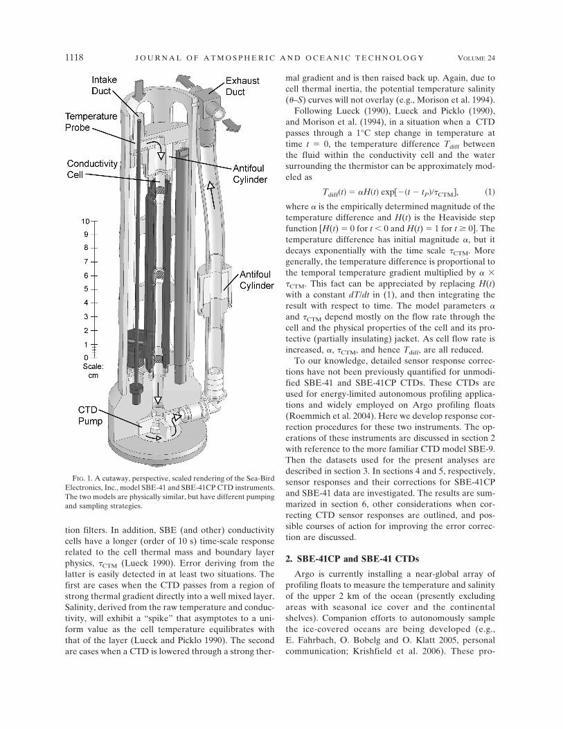
regular time grid (we chose 1 Hz for our calculations)before estimating model coefficients and applying thesecorrections to the data. Once the corrections were ap-plied to the 1-Hz dataset, the corrected dataset wasreinterpolated back to the original resolution. The op-timal correction adjusts salinity so that the mixed layerprofile is close to being statically stable (Fig. 11).

After discarding profiles for which our scheme re-turned improbable model coefficients, 115 and 342 pro-files were selected from the floats deployed by NOAA/PMEL and by UW, respectively (Fig. 12). The medianvalue of �CTM for the NOAA/PMEL floats is 20 s, withan interquartile spread of 24 s, and that of the UWfloats is 16 s, with an interquartile spread of 32 s. Themedian value of for the NOAA/PMEL floats is 0.023,with an interquartile spread of 0.019, and that for theUW floats is 0.028, with an interquartile spread of0.011. These SBE-41 model parameters have a largerspread than those derived for the SBE-41CP datasets.This difference in spread reflects greater uncertainty inthe values deduced for the SBE-41 sensors due to its

very infrequent sampling. Interestingly, the product ofthe median and �CTM for the two groups of SBE-41profiles were very similar: 0.46 and 0.45 s.

Two notable features of the individual thermal masscoefficient estimates for the UW floats are a clusteringof s around 0.025 for �CTM values between 0 and 20 s,and a cluster of �CTM values around 20 s from � 0.025to higher values. These are manifestations of the mini-mization routine that was seeded with � 0.02 and�CTM � 25 s. For profiles with only one anomalous datapoint in the mixed layer, the estimation of two modelcoefficients becomes an underdetermined problem.The minimization in these instances tends to either in-crease or decrease �CTM while leaving the other vari-able virtually unchanged.

6. Discussion

Operationally, there remains the issue of repeatabil-ity for the sensor response coefficients for the SBE-41CP and SBE-41 CTDs (Table 1). For the three SBE-

FIG. 11. Raw salinity (plus signs at each data point connected by a line), corrected salinity (circles with a line) and potentialtemperature, � (Xs with a line), (°C) from profile 13 of Argo float World Meteorological Organization (WMO) ID 490017. The floatis a Webb Research Corporation APEX260 equipped with a Sea-Bird Electronics SBE-41 CTD. The profile was collected on 12 Oct2002 at 52.45°N, 160.27°W. The corrected salinity was derived using median conductivity cell thermal mass correction model coefficients � 0.0267 and � � 18.6 s.


41CP CTDs analyzed, the weighted interquartilespread of thermistor lag �T is about a sixth and the totalspread of median lags (0.03 s) only about a tenth of theweighted median, indicating that the thermistor timeconstant is well determined and reasonably consistent.The weighted interquartile spread of median time shiftfor conductivity relative to temperature tP is about thesame size as the weighted median, and the total spreadof the medians time shifts (0.09 s) is even larger. Theseresults suggest that if the thermistor lag has been cor-rected, a time shift of conductivity may not be war-ranted. The weighted interquartile spread of the con-ductivity thermal mass time scale �CTM is about a fifthand the total spread of median values (1.68 s) about a

fourth of the median value, suggesting that it is fairlywell determined. The weighted interquartile spread andthe total spread of median amplitudes (0.045) for thecorrection amplitude are again about a seventh and afourth of the median value, suggesting that it is fairlywell determined.

For the SBE-41 data analyzed, the sampling is toocoarse to allow thermistor response correction or atime shift of conductivity relative to temperature. Theweighted interquartile spread of the conductivity ther-mal mass time scale �CTM is similar to the median value(Table 1). The weighted interquartile spread of the cor-rection amplitude is about a third of the weightedmedian value. The large spreads for the SBE-41 cor-rection parameters most likely result from the effects ofcoarse temporal (hence vertical) sampling on estimat-ing these parameters for a given profile. Below, it isargued that application of the correction using coeffi-cient median values makes statistical sense, eventhough individual profiles may not be perfectly cor-rected.

The conductivity thermal mass effect amountsroughly to a 0.01 PSS-78 error in data from a SBE-41CPtransiting a 0.01°C s�1 temperature gradient. The errorwould be about 0.005 PSS-78 for an SBE-41 transitingthe same temperature gradient. Floats ascending at0.09 dbar s�1 through strong thermoclines can experi-ence temperature gradients as large as 0.1°C s�1, al-though such gradients are rare. Thus, conductivity cellthermal mass errors for SBE-41CP-equipped floatscould occasionally approach 0.1 PSS-78, and those forSBE-41-equipped floats might experience errors halfthat magnitude. Both these potential errors are welloutside the Argo salinity accuracy target of 0.01. Whilelarge gradients are rare, approximately half of thePMEL profiles analyzed here sampled a temperaturegradient of 0.02°C s�1 or more, a gradient sufficientlystrong that the thermal mass error approaches the Argosalinity accuracy specification in the thermocline evenfor an SBE-41-equipped float. Given the typical oceantemperature stratification of warm water overlyingcold, uncorrected data will tend to be biased freshwithin and just above the thermocline.

The SBE-41 temporal resolution is coarse and irregu-lar, and 1-Hz data are rarely reported from SBE-41CPCTDs on Argo floats. Sample times are rarely (if ever)reported. These practices complicate the correction ofconductivity thermal mass errors in several ways. First,the relationship between pressure and time must beestimated to transform the reported vertical tempera-ture gradient into a temporal gradient. For the APEXfloats analyzed here, a constant rise rate of 0.09 dbars�1 was assumed, even though the standard deviation of

TABLE 1. Weighted median values and interquartile spreads ofsensor response corrections for SBE-41CP and SBE-41 CTDs.

SBE-41CP CTD SBE-41 CTD

MedianInterquartile

spread MedianInterquartile

spread

�T (s) 0.39 0.07 N/A N/AtP (s) 0.05 0.04 N/A N/A�CTM (s) 6.68 1.31 18.6 19 0.141 0.019 0.0267 0.010

FIG. 12. Values of conductivity cell thermal mass correctionmodel parameters and �CTM for selected profiles from floatsdeployed by NOAA/PMEL (Xs) and by the University of Wash-ington (circles). In all instances data are from SBE-41 CTDsmounted on APEX floats. Medians (black symbols) and the in-terquartile ranges (gray ellipses) are plotted for both sets of floats.Curves for constant median values of � �CTM (thin black lines)are also displayed.


available rise rate estimates is �0.03 dbar s�1. This un-certainty introduces errors into the reconstructed tem-perature time history. In addition, the sparse verticalsampling (or resolution of reported data), only reachingas fine as 4–10 dbar in the upper ocean (correspondingto time intervals of 44–110 s), means that the time his-tory of temperature is grossly underreported with re-spect to either model CTD’s conductivity cell thermalmass error time scale (roughly 7 s for the SBE-41CP,and 19 s for the SBE-41). This coarse sampling intro-duces more uncertainty into the correction by aliasingtemperature variations on shorter time scales than thesampling (or averaging, or subsampling) interval intothe gradient estimates. Because of these uncertainties,we believe that a realistic confidence limit on the esti-mated corrections is about the magnitude of the cor-rections themselves. That is, we can remove bias in thereported salinity owing to the conductivity cell thermalmass error, but a conservative assessment of the uncer-tainty in the corrected salinity for any individual datapoint is thought to be about the magnitude of the cor-rection itself.

Even if the correction is uncertain from point topoint, an overall statistical salinity bias will still remainfor uncorrected profiles, especially in and above thethermocline, owing to the large-scale vertical tempera-ture gradient there. Hence, it makes sense to apply thecorrection to remove this bias in a statistical sense evenif the available profile data are not optimum for thecorrection. To apply the correction following conven-tional methods (Lueck and Picklo 1990; Morison et al.1994) it is best to first convert the temperature datafrom a function of pressure to one of time using the bestavailable estimate of float ascent rate, to interpolate thedata to a uniform (e.g., 1 Hz) time series, to apply thecorrections, and then to decimate back to the originalresolution.

Often SBE-41 CTD equipped floats are programmedto sample at finer pressure intervals near the surfacethan at depth. Given the different heat exchange char-acteristics for the SBE-41 when the pump is on versuswhen it is off, the conductivity cell thermal mass errorfor the SBE-41 might be sensitive to the sample sched-ule. Here the SBE-41 correction coefficients were de-termined using upper-ocean data from one dataset hav-ing 4–8-dbar resolution (NOAA/PMEL) and anotherwith 10-dbar intervals (UW). It is reassuring that re-sulting coefficients from our analyses are in roughagreement. Application of the method to other floatdatasets in which SBE-41 CTDs were programmed tosample at significantly different intervals might revealhow the error model coefficients vary with varying sam-pling intervals.

We note that the SBE-41CP data used to estimatethe conductivity cell thermal inertia correction coeffi-cients for that instrument were from ITPs that rise atabout 0.27 dbar s�1, a rate about 3 times that of profil-ing CTD floats. Our analysis of the ITP data may tendto underestimate the SBE-41CP correction coefficientsfor float applications for two reasons. First, althoughthe CTD conductivity cells are encased in a polyure-thane jacket that is relatively insulating compared withthe glass itself, some heat is still exchanged between theconductivity cell and the external water. This exchangewill increase as the flow past the exterior of the cellincreases (Lueck 1990). In addition, because the ductintakes of SBE-41 and SBE-41CP CTDs face up whilethe exhaust ports are oriented perpendicular to the in-takes, there is a pressure differential between intakeand exhaust that varies with ascent rate. At a 0.09 dbars�1 ascent speed, the pressure-induced flow velocity inthe duct with the pump off may be about 0.008 m s�1,but at triple the ascent speed, this flow velocity could be9 times larger, or about 0.07 m s�1. This value is morethan a tenth of the estimated pumped flow of 0.64 m s�1

for the SBE-41CP. Thus, the ITP-mounted SBE-41CPsmay have smaller conductivity cell thermal inertia er-rors than float-mounted SBE-41CPs. It would be in-structive to deploy a profiling CTD float equipped witha SBE-41CP in a region of thermohaline staircases andtelemeter back full-resolution data to check (and per-haps revise) the model coefficients estimated here.

A few modifications could be made to existing tech-nology to reduce uncertainty in the conductivity cellthermal mass corrections. First, the float buoyancy en-gine software could be modified to produce a known,relatively uniform ascent rate, reducing the error in es-timating the time history of temperature sampled bythe floats. Alternately, the floats could report sampletime in addition to temperature, salinity, and pressure.Second, reporting data at increased temporal (hencevertical) resolution would result in improved ability toreduce the uncertainty of the corrected salinities. In-creased vertical resolution should be more easily real-ized with floats that communicate through Iridium.Third, SBE-41CP software could be modified to applythe sensor response corrections estimated here to thefull-resolution 1-Hz data prior to bin averaging or sub-sampling the data. But before this step is taken, itwould be prudent to estimate the SBE-41CP correctioncoefficients at typical float rise rates. To improve sensorresponse corrections, one might profile different mod-els of CTDs through thermohaline staircases at a vari-ety of ascent speeds and pump rates. It would also bedesirable to determine how the correction coefficientsvary with varying rise rates.


Acknowledgments. The National Ocean PartnershipProgram and the National Oceanic and AtmosphericAdministration (NOAA) Office of Oceanic and Atmo-spheric Research funded this analysis. The ITP datawere acquired under National Science Foundation(NSF) Grant OCE0324233. Dr. Donald Denbo pointedout the artifacts in the float data resulting from con-ductivity cell thermal mass error. Dr. Elizabeth Steffenhelped with (unpublished) laboratory investigations ofthe SBE-41 CTD conductivity cell response to tempera-ture changes. Comments by Hugh Milburn, James Th-ompson, and two anonymous reviewers helped to im-prove the final version of this manuscript. The floatdata used herein were collected and made freely avail-able by Argo (a pilot program of the Global OceanObserving System) and the national programs that con-tribute to it (see online at http://www.argo.net/). Anyopinions, findings, and conclusions or recommenda-tions expressed in this material are those of the authorsand do not necessarily reflect the views of NSF orNOAA. The mention of a commercial product hereindoes not constitute endorsement by NOAA or NSF.

REFERENCES

Fofonoff, N. P., S. P. Hayes, and R. C. Millard Jr., 1974: W.H.O.I./Brown CTD microprofiler: Methods of calibration and datahandling. Woods Hole Oceanographic Institution Tech. Rep.WHOI-74-89, 64 pp.

Gregg, M. C., and W. C. Hess, 1985: Dynamic response calibra-tion of Sea-Bird temperature and conductivity probes. J. At-mos. Oceanic Technol., 2, 304–313.

Krishfield, R., and Coauthors, 2006: Design and operation of au-tomated Ice-Tethered Profilers for real-time seawater obser-vations in the polar oceans. Woods Hole Oceanographic In-stitution Tech. Rep. WHOI-2006-NN, 30 pp.

Lueck, R. G., 1990: Thermal inertia of conductivity cells: Theory.J. Atmos. Oceanic Technol., 7, 741–755.

——, and J. L. Picklo, 1990: Thermal inertia of conductivity cells:Observations with a Sea-Bird cell. J. Atmos. Oceanic Tech-nol., 7, 756–768.

Morison, J., R. Andersen, N. Larson, E. D’Asaro, and T. Boyd,1994: The correction for thermal-lag effects in Sea-Bird CTDdata. J. Atmos. Oceanic Technol., 11, 1151–1164.

Roemmich, D., S. Riser, R. Davis, and Y. Desaubies, 2004: Au-tonomous profiling floats: Workhorse for broadscale oceanobservations. J. Mar. Technol. Soc., 38, 31–39.

Ruddick, B., 1983: A practical indicator of the stability of thewater column to double-diffusive activity. Deep-Sea Res.,30A, 1105–1107.


Documents

Sensor Corrections for Sea-Bird SBE-41CP and SBE-41 CTDs*