1

Sensitivity of Nocturnal Boundary Layer to Tropospheric Aerosol Radiative Forcing Under Clear Sky Conditions

Udaysankar S. Nair1, Richard McNider2, Falguni Patadia1, Sundar A. Christopher1,2 and

Kirk Fuller1

1Earth System Science Center, University of Alabama in Huntsville, 320 Sparkman Drive

Huntsville, Alabama 35805

2Department of Atmospheric Science, University of Alabama in Huntsville

320 Sparkman Drive

Huntsville, Alabama 35805

Journal of Geophysical Research

December 17, 2009

Revised, February 17, 2010

1 Corresponding Author: U.S. Nair, Earth System Science Center, University of Alabama in Huntsville, Huntsville, AL 35805 E-mail: nair@nsstc.uah.edu Phone: 256-961-7841

0

ABSTRACT 1 2

Since the middle of the last century, global surface air temperature exhibits an increasing trend, 3

with nocturnal temperatures increasing at a much higher rate. Proposed causative mechanisms 4

include the radiative impact of atmospheric aerosols on the nocturnal boundary layer (NBL) 5

where the temperature response is amplified due to shallow depth and its sensitivity to potential 6

destabilization. A one-dimensional version of the Regional Atmospheric Modeling System 7

(RAMS) is used to examine the sensitivity of the nocturnal boundary layer temperature to 8

surface longwave radiative forcing (SLWRF) from urban aerosol loading and doubled 9

atmospheric carbon dioxide concentrations, for typical mid-latitude nocturnal boundary layer 10

case days from the CASES-99 field experiment. The analysis is further extended to urban sites 11

in Pune and New Delhi, India. For the cases studies, locally the nocturnal SLWRF from urban 12

atmospheric aerosols (2.7 – 30 W m-2) is comparable or exceeds that caused by doubled 13

atmospheric carbon dioxide (3 W m-2), with the surface temperature response ranging from a 14

compensation for daytime cooling to an increase in the nocturnal minimum temperature. The 15

sensitivity of the NBL to radiative forcing is approximately four times higher compared to the 16

daytime boundary layer. Nighttime warming or cooling may occur depending on the nature of 17

diurnal variations in aerosol optical depth (AOD). Soil moisture also modulates the magnitude 18

of SLWRF, decreasing from 3 W m-2 to 1 W m-2 when soil saturation increases from 37% to 19

70%. These results show the importance of aerosols on the radiative balance of the climate 20

system. 21

1

1 Introduction 22

Surface air temperature observations in the last century show a clear trend of 23

nighttime minimum temperatures increasing at a rate twice that of the daytime maximum 24

temperature except during the 1979-2004 time period when the rate of increase of both 25

maximum and minimum temperatures are approximately the same [Dai et al. 1999; Karl 26

et al. 1984, 1993]. This asymmetry in the trends of maximum and minimum temperatures 27

have decreased the diurnal temperature range (DTR) over the land surface throughout the 28

globe with the exception of weak increases in central Canada and southeastern Australia 29

[Karl et al. 1993]. While the DTR decrease is present in every season, in most areas the 30

largest decreases occur during the Northern Hemisphere Summer and Fall seasons. There 31

is considerable debate regarding the mechanisms responsible for the DTR decrease 32

[IPCC 2007; Dai et al. 1999]. Some suggested factors responsible for this increase 33

include urban heat islands, greenhouse gases, clouds, land use changes, and tropospheric 34

aerosols [Balling et al., 2003, Braganza et al., 2004a; Kalnay and Cai, 2003; Pielke et 35

al., 2007; Zhou et al., 2007]. Heat island effects would initially appear to be a viable 36

mechanism because minimum temperatures are more susceptible to urban thermal inertia. 37

However, DTR climate trend analyses often attempt to remove these urban effects [Karl 38

et al., 1984]. 39

Global Circulation Model (GCM) sensitivity studies show that increased 40

concentration of greenhouse gases such as CO2 and CH4 also cause changes in DTR. 41

However, comparative studies with state-of-the-art GCMs reveal differences in the 42

magnitude and even the sign of DTR trends among the models. These studies also reveal 43

large discrepancies between modeled and observed DTR trends [Karl et al., 1993]. Based 44

2

on these results, Karl et al. [1993] and Stone and Weaver [2003] concluded that the land 45

surface parameterizations or physics in existing GCMs may not be robust enough to 46

correctly capture the observed DTR signal. Walters et al. [2007] also proposed that the 47

coarse resolution in GCMs may not correctly capture the sensitivity of the nocturnal 48

boundary layer to either external forcing or parameters describing the land surface 49

characteristics. 50

Cloudiness trend is another factor that needs to be considered in interpreting 51

observed DTR trends. Dai et al. [1999] examined the physical and statistical relationships 52

of clouds, precipitation, and soil moisture in the First International Satellite Land Surface 53

Climatology Project (ISLCP) Field Experiment (FIFE) data. They showed that clouds 54

could change the DTR, and that soil moisture was less important than clouds. Using this 55

evidence, and some historical measures of cloudiness trends, they concluded that 56

cloudiness was the most likely cause of the DTR change. Hansen et al. [1995] showed 57

that clouds were apparently the only adjustable GCM parameter that could damp the 58

DTR to its observed magnitude. However, the GCMs often lack adequate vertical 59

resolution in the nocturnal boundary layer (NBL) and do not include explicit treatment of 60

aerosol microphysics. As will be shown in this paper, aerosols would provide a similar 61

response signal to that of a change in cloudiness. Further, while cloudiness trends are 62

uncertain, anthropogenic aerosol loading in the atmosphere has definitively increased in 63

the last century [Ramanathan et al., 2001a]. Recently, [Kalnay and Cai, 2003] conducted 64

a long-term reanalysis of modeled and observed data. This study showed that changes in 65

land surface usage, including irrigation, contribute significantly to the observed DTR 66

trends. Irrigation would have the expected effect of lowering daytime temperatures due to 67

3

evaporation, and raising nighttime temperatures due to the higher heat capacity of wet 68

soils and well-hydrated vegetation. However, rigorous statistical verification of this 69

mechanism would be difficult because surface moisture availability is not routinely 70

measured. Moreover, the DTR has decreased in some areas where irrigation effects 71

would be minimal, such as the eastern United States. All in all, with the uncertainties in 72

long-term cloudiness trends and the persistent deficiencies in GCM surface land 73

processes, there is still considerable uncertainty in explaining the DTR trends. 74

Increases in tropospheric aerosol concentrations have also been suggested as a 75

significant factor in the DTR trends [Stone and Weaver, 2003; Braganza et al., 2004a, 76

2004b; Makowski et al., 2008]. Makowski et al. [2008] attributes long-term trends in 77

DTR mostly to modulation of incoming solar radiation through the direct and indirect 78

aerosol effect. Most aerosol studies [IPCC, 2007] have concentrated on the direct 79

radiative effect of aerosol scattering and the indirect effects of aerosols in clouds [see Yu 80

et al., 2002 for a comprehensive review]. Both effects tend to increase the planetary 81

albedo and reduce daytime temperatures. Recent global-scale aerosol studies [Koch et al., 82

2007] have begun to demonstrate the importance of carbonaceous aerosols, especially 83

elemental carbon (EC), to the atmospheric aerosol budget. EC aerosols serve as net 84

warmers of the planetary boundary layer (PBL) and the free troposphere. This effect 85

would counter aerosol cooling in the daytime and reduce surface cooling at night. 86

Detailed reviews of aerosol measurement and modeling studies [IPCC, 2007] have 87

concluded that the foregoing aerosol effects are potentially significant (with magnitudes 88

comparable to the predicted warming from greenhouse gases), but also very poorly 89

4

understood (the magnitude of the net uncertainty is comparable to the aerosol effects; the 90

sign is unknown). 91

The majority of research studies on aerosol radiative interactions focus on the 92

daytime interaction of aerosols with solar radiation through both direct and indirect 93

pathways. However, there are relatively few studies that address the radiative impact of 94

aerosols on the nocturnal boundary layer [Estournel et al., 1983; Garratt et al., 1990; 95

Jacobson, 1997; Venkatram and Viskanta, 1977; Yu et al., 2002; Zdunkowski et al., 96

1976]. Even though these studies address various aspects of aerosol radiative interaction 97

with NBL, a systematic analysis that includes spatio-temporal variations of the NBL and 98

aerosols is lacking. Zdunkowski et al. [1976] conducted a detailed analysis of the impact 99

of air pollution on PBL including the hygroscopic growth of aerosols. While the 100

numerical modeling experiments of Zdunkowski et al. [1976] did not explicitly consider 101

effects of diurnal asymmetries in atmospheric aerosol loading [diurnal variations in 102

aerosol optical depth (AOD) resulting from changes in aerosol mass concentration, 103

chemical composition, particle size, etc.], they noted that dense haze cover at nighttime 104

following a clear day will lead to warming at the surface. Jacobson [1997] used a detailed 105

air pollution modeling system to examine the impact of aerosols on the PBL, including 106

the nocturnal effects. Even though the modeling system captured the diurnal variability of 107

aerosol loading, the study did not focus on the role of nocturnal heating and DTR trends. 108

It is the purpose of this study to investigate the response of the nocturnal boundary 109

layer to longwave aerosol radiative forcing. Simple models [Pielke and Matsui, 2005] 110

have indicated that due to the shallow nature of the nocturnal boundary layer under light 111

winds, the temperature response to longwave forcing may be large. Additionally, 112

5

Walters et al. [2007] showed that the forcing itself may change the boundary layer height 113

causing a mixing of heat down from aloft. This mixing of heat from aloft acts as a 114

multiplier effect to the direct warming due to the added radiation. While both of these 115

studies dealt with increases in downward longwave radiation into the surface from 116

greenhouse gases, similar responses might be expected from downward longwave 117

radiation to the surface from aerosols. Also, both of these studies employed simple 118

models. Pielke and Matsui [2005] employed a semi-empirical analytical formulation that 119

did not incorporate full nonlinear dynamics between the surface and the atmosphere. 120

Walters et al. [2007], while including full nonlinear interaction with the surface, only 121

employed a two-layer atmosphere. The present study will examine the response of a full 122

nonlinear multi-level atmospheric model (a one-dimensional version of the Regional 123

Atmospheric Modeling System - RAMS) to aerosol radiative forcing. The experimental 124

design and description of the numerical modeling system used are described in section 2, 125

while results, discussion of the analysis and conclusions are presented in sections 3, 4 and 126

5 respectively. 127

2 Methodology 128

2.1 Experimental Design 129

The primary goal of this study is to assess the immediate direct effect of surface 130

longwave radiative forcing (SLWRF) from urban aerosols on nighttime surface air 131

temperatures and gain an understanding of conditions and processes through which 132

surface air temperature is impacted. Also of interest is to compare the impact of SLWRF 133

from atmospheric aerosols to doubled atmospheric carbon-dioxide. This is achieved by 134

conducting sensitivity analysis on typical cases of observed, stable nocturnal boundary 135

6

layer (SNBL) development using a one-dimensional version of RAMS. While this study 136

is a sensitivity analysis, it is important to note that the experiments are based on a 137

nocturnal boundary layer that has the physical attributes of observations. As noted by 138

Steeneveld et al. [2006] and Walters et al. [2007], models often have difficulties 139

capturing the dynamic range of boundary layer cooling at night due to anomalous 140

numerical diffusion or profile formulations that preclude strong stability. Such models 141

will not be sensitive in resolving the effects of relatively small perturbations in longwave 142

radiation at the surface. Thus, this study adopts an experimental design where RAMS is 143

used to simulate typical SNBL case study days of 21-22 October 1999 from the 144

Cooperative Atmosphere-Surface Exchange Study [Poulos et al., 2002] held in 1999 145

(CASES-99) near Leon, Kansas (37.65°N, 96.73°W) with the objective of improving the 146

understanding of processes relevant to the SNBL. The days used in this study are typical 147

SNBL case days that are the focus of other modeling studies [Steeneveld et al., 2006]. 148

The experimental design utilized in this study establishes the capability of the model to 149

faithfully simulate these typical SNBL case days by comparing model simulations against 150

detailed field observations of surface meteorology and energy fluxes collected during 151

CASES-99. 152

Sensitivity experiments are then conducted for these case days by modifying the 153

validated control experiment (C1), by including radiative forcing from typical urban 154

aerosols (U1) and doubled atmospheric carbon dioxide (X2, see Table 1 for description of 155

all the experiments). Additional sensitivity experiments, U2 and U3 are conducted to 156

examine the impact of diurnal variation in atmospheric aerosol loading, D1 to address the 157

impact of other aerosol types on SNBL development, while C2 and U4 are used to 158

7

examine how soil moisture modulates the impact of aerosol surface radiative forcing on 159

surface air temperature. 160

The analysis is then extended to urban locations where detailed observations are 161

not available for initialization and validation, but for which aerosol characterization is 162

available. The experiments U5 and U6, utilize urban aerosol composition characteristic 163

of two urban sites in India, namely Pune [Panicker et al., 2008] and New Delhi [Singh et 164

al., 2005] respectively, valid for the time period December 2004-January 2005 and April-165

June, 2003 respectively. The U5 and U6 experiments are compared against C3 and C4 166

which are experiments that are identical to U5 and U6, except for the assumption of clear 167

air conditions in order to examine whether the results obtained for CASES-99 site is also 168

applicable to other areas. 169

Note that the experiments used in this study are not climate experiments since 170

they do not look at the cumulative impact of either aerosols or greenhouse gases. Rather, 171

they provide an examination of the direct sensitivity of NBL to these forcings. 172

2.2 Description of RAMS 173

This study utilizes RAMS, Version 4.4, modified to include radiative interactions 174

of aerosols, to study the impact of aerosols on nocturnal boundary layer development. 175

RAMS is a nonhydrostatic atmospheric model used to simulate a wide range of 176

atmospheric phenomenon [Cotton et al., 2003] and utilizes finite difference 177

approximations to solve conservation equations of mass, momentum, heat, and different 178

water phases. Cloud and precipitation processes are represented in the model through 179

either convective parameterization or explicit parameterization of cloud microphysics. 180

RAMS provides a variety of options with varying sophistication for representing subgrid-181

8

scale turbulence. Land surface processes are simulated using a multi-layer soil model 182

and the Land Ecosystem Atmosphere Feedback (LEAF-2) model [Walko et al., 2000]. 183

While radiative transfer schemes of varying complexity [Mahrer and Pielke, 1977; Chen 184

and Cotton, 1983; Harrington et al., 1999] are available in RAMS, none account for 185

radiative interactions with aerosols. RAMS was modified to include a Delta four-stream 186

radiative transfer scheme of Fu and Liou [1993], referred from hereon as FL-RTS [Wang 187

and Christopher, 2006; Wang et al., 2006]. Aerosol characterization within FL-RTS is 188

based on the Optical Properties of Aerosols and Clouds (OPAC) based on Hess et al. 189

[1998]. 190

2.2.1 The FL-RTS 191

The FL-RTS is a plane-parallel radiative transfer model [Fu and Liou, 1993] that 192

computes upwelling and downwelling radiative fluxes at specified, discrete locations 193

within an atmospheric column. The FL-RTS divides the radiation spectrum into six 194

broadbands in the shortwave (SW) part (0.2-4 μm), with the first bands (0.2-0.7 μm) 195

being subdivided into ten subbands. The longwave (LW) part of the spectrum (4-37.5 196

μm) is subdivided into twelve broadbands. Gaseous absorption characteristics within 197

these bands are computed using the correlated k-distribution method [Fu and Liou, 1992]. 198

A delta function is used to model the forward scattering by clouds and aerosols. The FL-199

RTS provides the option to be configured either in the two or four stream mode for 200

radiative flux computations. Fu and Liou [1993] show that the FL-RTS irradiance 201

estimates are within 0.05% of line-by-line calculations. 202

9

2.2.2 The OPAC Aerosol Types 203

The OPAC is a software package for specifying optical properties of clouds and 204

aerosols as a function of wavelength. Single scattering albedo (ωo), asymmetry parameter 205

(g) and extinction coefficient (βext), for individual aerosol components and aerosol types 206

(mixture of components), are available at 61 wavelengths between 0.25 and 40 μm and at 207

eight relative humidity values between 0–99%. These optical properties along with 208

vertical distribution information are needed to specify aerosol radiative interactions in the 209

model. The OPAC assumes a lognormal size distribution for aerosols and optical 210

properties of individual components are computed assuming number concentrations of 1 211

cm-3 and therefore require appropriate scaling for differing situations. Aerosol types in 212

OPAC range from clean and polluted continental conditions to Arctic and Antarctic types 213

which are composed of specific mixes of individual components. The OPAC aerosol 214

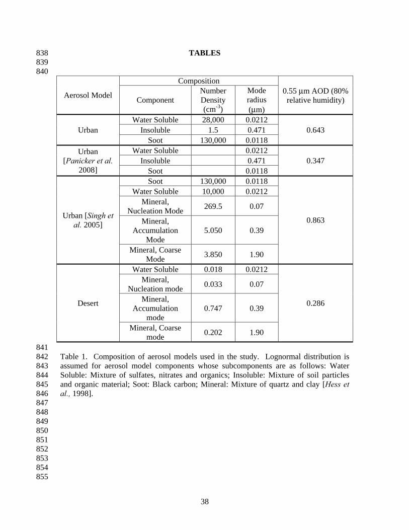
types utilized in this study, namely Urban and Desert types differ both in composition 215

and microphysics (Table 2). Urban aerosol types have relatively high number 216

concentrations of water soluble and soot components, but smaller particle sizes in 217

comparison to desert aerosol types dominated by accumulation and coarse mode mineral 218

components (see Table 2). This study specifically focuses on Urban and Dust aerosol 219

types since prior studies report substantial SLWRF associated with these aerosol types 220

and thus the potential to impact SNBL evolution. The other two aerosol types considered 221

in study are essentially OPAC aerosol types modified to conform to characteristics of 222

urban aerosols observed over Pune and New Delhi, India, as reported in Panicker et al. 223

[2008] and Singh et al. [2005]. The aerosol type for Pune, India, valid for the time period 224

December 2003 through January 2004, is the OPAC Urban type with the number density 225

10

of the components modified (Table 2) to match the observed AOD, Single Scattering 226

Albedo (SSA) and Asymmetry Parameter (ASP). Using a similar approach, Singh et al. 227

[2005] found the pre-monsoon aerosol characteristics to be a mixture of the OPAC Urban 228

and Desert aerosol types (Table 2). 229

2.2.3 Calculation of Aerosol Optical Thickness 230

Aerosol Optical Depth (AOD) is computed following Hess et al. [1998] by 231

assuming exponentially decreasing number concentrations with height as given by 232

equation 1: 233

Hz

eNzN−

= )0()( (1) 234

where z is the altitude above ground in kilometers and H is the scale height in kilometers. 235

The scale height specifies the nature of decrease of number concentration with height, 236

with increasing values describing smaller variation with height. Based on aerosol vertical 237

distribution described by (1), AOD of an atmospheric layer contained between height 238

levels z1 and z2 (z1 < z2) is given by: 239

⎟⎟⎠

⎞⎜⎜⎝

⎛−====

−−−

∫ Hz

Hz

ext

z

z

Hz

ext eeHRHzdzeRHzzz212

1

),,0(),,0(),( 21 λβλβτ λ (2) 240

where λ is the wavelength, RH is relative humidity. For each aerosol type, OPAC outputs 241

βext at z = 0, computed using specified number concentrations of individual components. 242

OPAC specifies the total physical thickness of Urban and Desert aerosol layers as 2 and 6 243

km and the scale heights to be 8 and 2 km respectively. Based on these parameters, the 244

computed values of AOD at 0.55 μm and 80% RH for Urban and Desert aerosol types are 245

0.643 and 0.286, respectively. The OPAC Urban AOD is consistent with values over 246

11

polluted regions in Africa, India, and China [Ramanathan et al., 2001b; Smirnov et al., 247

2002; Pandithurai et al., 2007]. Since OPAC provides the optical properties only at eight 248

discrete RH values, linear interpolation is used to determine aerosol optical properties at 249

other RH values. Note, in addition to the mixed layer aerosol types, OPAC also suggests 250

the use of a background aerosol type for the free troposphere (τ ~ 0.013), stratospheric 251

aerosol layer (τ ~ 0.005), and if applicable, a transported mineral aerosol layer (τ ~ 252

0.097). In this study, only the impact of the boundary layer aerosols is considered and the 253

effect of other categories is ignored. 254

2.3 Numerical Model Configuration 255

Numerical experiments consist of 1D simulations of atmospheric boundary layer 256

development over a 48-hour period starting from initial conditions characterized by 257

evening radiosonde observations. A pseudo one-dimensional configuration of RAMS to 258

simulate atmospheric boundary layer development using a domain of 5 × 5 grid points is 259

used with cyclic boundary conditions along the lateral boundaries. A sufficiently large 260

grid spacing of 10 km in the x and y directions is utilized so that the model is incapable 261

of resolving large eddies. Vertical grid structure, surface characteristics, and other 262

relevant information are provided in Table 3. 263

For the CASES-99 case days, when the soil model is directly initialized using soil 264

moisture observations, model-simulated latent heat fluxes are negligible compared to 265

observations. Latent heat flux observations are not negligible however, and thus suggest 266

that while the local soil moisture observations in the 0–25 cm layer are dry, it may not be 267

reflective of large-scale conditions. Therefore the soil moisture content in this layer was 268

systematically altered until close agreement was obtained between observations and 269

12

model-simulated sensible and latent heat fluxes, 2 m temperature, and relative humidity. 270

The altered soil moisture profile was utilized in all the other experiments. 271

In the urban site experiments (U5-U6), soil moisture and temperature 272

observations are not available and therefore information from the National Center for 273

Environmental Prediction (NCEP) Reanalysis dataset was utilized to initialize the soil 274

model. Note that the soil moisture values from the NCEP Reanalysis are average 275

conditions for 2.5 × 2.5 degree grid cell. Similar to C1 experiment, the soil moisture was 276

adjusted until there was relatively good agreement between the observed 2 m temperature 277

and relative humidity is obtained for U5 and U6 experiments. 278

3 Results 279

The sensitivity analyses discussed in the following sections utilize specific days 280

from CASES-99 (21-22 October 1999). Additional experiments conducted for the time 281

period 23-25 October 1999 CASES-99 days yielded similar results and thus are excluded 282

for brevity. 283

3.1 Comparison of the CASES-99 Control Simulation to Observations 284

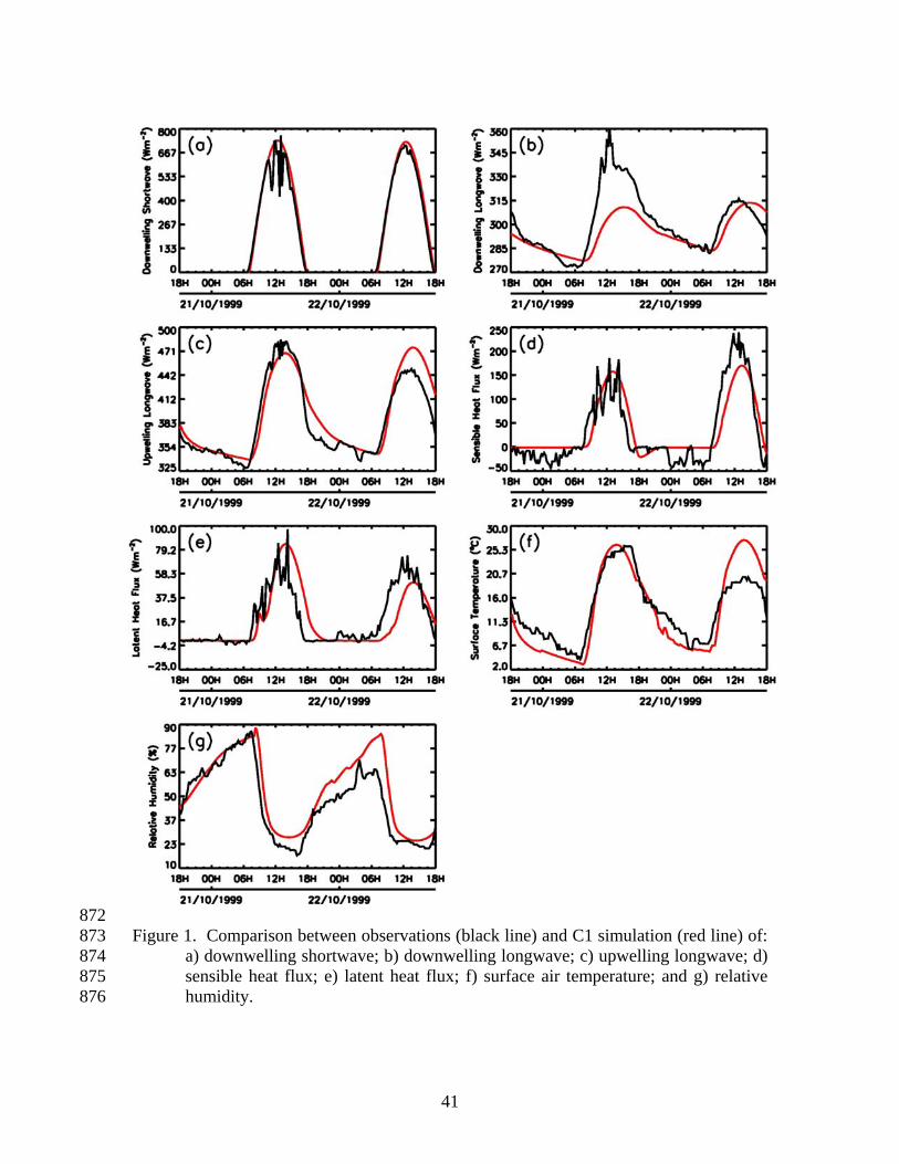
Observations of downwelling solar radiation (Figure 1a) show the presence of 285

clouds in the time period centered around local solar noon on both 21 and 22 October 286

1999 making comparisons to model simulations complicated. Cloud cover appears to be 287

more optically thick and persistent on 21 October when compared to 22 October. 288

Comparison to observations on the 22 October shows the FL-RTS generally 289

overestimating the downwelling shortwave with a maximum difference of 61 W m-2. 290

During the late afternoon hours for both days, when clouds are not present, mean error 291

13

between model simulation and observations is approximately 5%, slightly higher than the 292

than the 3% error estimated by Christopher et al. [2003]. 293

Downwelling longwave radiation at the surface (Figure 1b) from FL-RTS 294

compare well with observations during both nights (differences of less than 2%), while 295

there are considerable differences during the first day (maximum of 18%). Significant 296

daytime differences during the first day may be related to the presence of clouds. During 297

the second night, there is again close agreement between model and observations with 298

differences averaging less than 2%. During the second day, there is better agreement 299

between the simulation and observations during the morning hours, but larger deviations 300

in the afternoon. However, note that there was a frontal passage through the area at this 301

time which the model does not capture. 302

There is good agreement between the observed and model-simulated upwelling 303

longwave radiation from the surface (Figure 1c), except during the afternoon hours of the 304

second day when the frontal passage occurred. Simulated patterns of surface sensible and 305

latent heat fluxes (Figure 1d,1e), though very similar to observations, lag the observations 306

by approximately half an hour. The heat and moisture fluxes show significant variability 307

during the first day due to cloudiness. During the second day, the variability is much less 308

and the maximum amplitudes of observed and simulated patterns of sensible and latent 309

heat fluxes differ by ~40 W m-2 and 15 W m-2 respectively. The RAMS simulations of 310

temperature and humidity patterns are also consistent with observations during the first 311

day, but differ during the second day due to frontal passage. 312

14

3.2 Radiative Impact of Urban Aerosols and Doubled Carbon Dioxide 313

While top-of-atmosphere shortwave and longwave radiative forcing metrics are 314

utilized in Earth radiation budget studies, radiative forcing at the surface is the metric that 315

is most relevant for this study. For given land surface conditions, the surface air 316

temperature, heat, and moisture fluxes to the atmosphere are most sensitive to net 317

radiative energy available at the surface. Thus surface shortwave and longwave radiative 318

forcing are the appropriate metrics for analyzing the impact of atmospheric aerosols on 319

boundary layer development and will be utilized in the analysis of the experiments 320

conducted in this study. 321

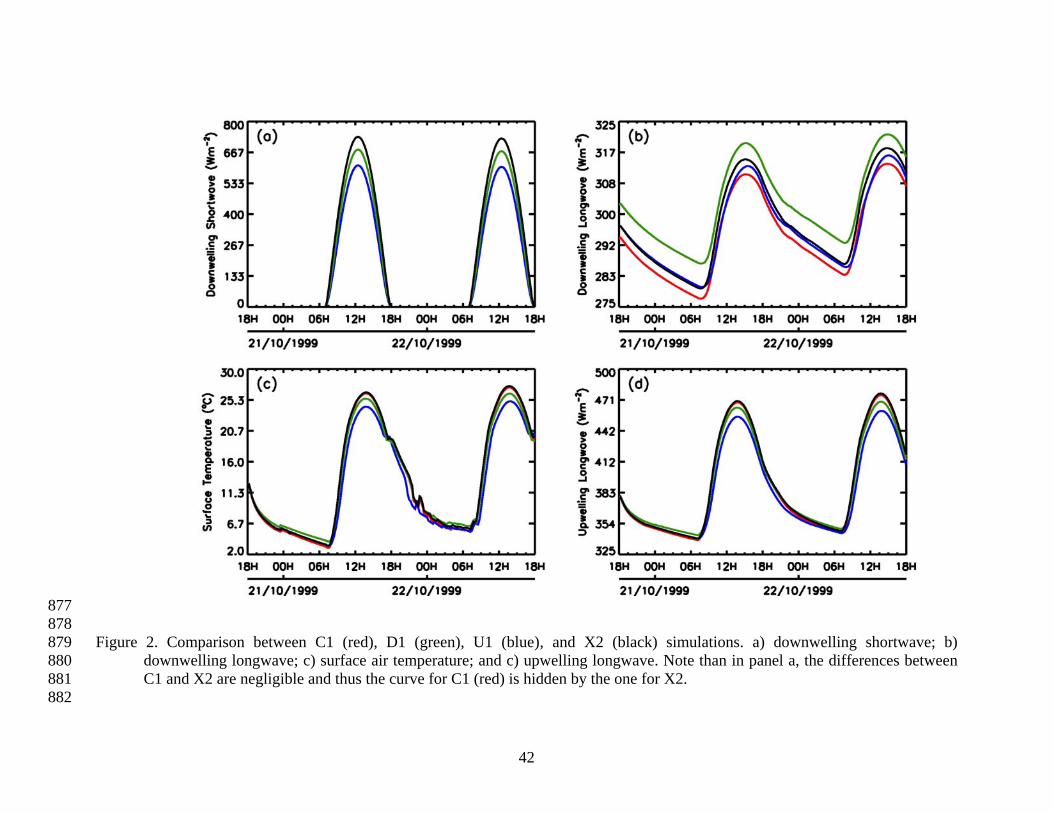
In the shortwave part of the spectrum, when comparing the control (C1), urban 322

aerosol (U1) and doubled CO2 experiments (X2), significant differences are observed 323

only between the C1 and U1 experiments (Figure 2a). The downwelling shortwave 324

radiation at the surface is significantly reduced in the U1 experiment, with differences of 325

up to 123 W m-2 occurring at the local solar noon hour. Since carbon dioxide is not a 326

major absorber in the shortwave, there is very little difference in the downwelling 327

shortwave flux at the surface between the X2 and C1 experiment. 328

However in the longwave there are significant differences between the U1, X2, 329

and the C1 experiment (Figure 2b). During the first night, both U1 and X2 show 330

enhancement in downwelling longwave of approximately 3.0 W m-2 compared to the C1 331

experiment. During the second night, the enhancement in downwelling longwave in the 332

U1 simulation reduces to ~2.2 W m-2. This reduction during the second night is related to 333

reduced water vapor loading in the U1 simulation due to attenuation of downwelling 334

shortwave radiation leading to less evaporation and transpiration. The nocturnal 335

enhancement in downwelling longwave radiation is within the range (2.5 to 16 W m-2) 336

15

reported by prior studies [Estournel et al., 1983; Jacobson, 1997; Panicker et al., 2008; 337

Zdunkowski et al., 1976], closer to lower limits. The nighttime differences in 338

downwelling longwave between U1 and X2 are minimal during the first night (~0.1–0.2 339

W m-2) and are more significant during the second night (~1 W m-2). During the daytime, 340

the differences in downwelling longwave between the C1 and U1 simulations are 341

significantly greater with a maximum value of approximately 4.5 W m-2 reflecting 342

differing vertical distributions of aerosols and carbon dioxide. Note that the urban 343

aerosols are confined to the lowest 2 km while carbon dioxide is assumed to be well 344

mixed through the depth of the model atmosphere. Thus, under clear-sky conditions, 345

carbon dioxide is able to better absorb and reradiate enhanced longwave emissions from 346

the surface and the PBL during the daytime. 347

3.3 Impact of Urban Aerosols and Doubled Carbon Dioxide on Surface Air 348 Temperature 349

In the CASES experiments, enhancement in nocturnal downwelling longwave 350

radiation due to urban aerosol loading and doubling of carbon dioxide leads to an 351

increase in surface air temperature during the first night (Figure 2c). The nocturnal 352

minimum is increased by ~0.38°C and 0.3°C during the first night in U1 and X2 353

experiments, respectively. During the first day of the simulation, significant reduction of 354

downwelling shortwave radiation at the surface is accompanied by reduction in daytime 355

surface air temperature in the U1 experiment with a maximum difference of ~2°C 356

occurring in the afternoon (Figure 3). The surface air temperature in the X2 simulation 357

shows a very small increase when compared to the C1 simulation, with a maximum 358

difference of less than 0.16°C (Figure 3) occurring in the afternoon. Note that the small 359

16

increase in daytime surface air temperature in the X2 experiment is primarily due to 360

enhancement in downwelling longwave radiation at the surface. 361

The impact of doubled carbon dioxide on surface air temperature during the 362

second night is very similar to that found during the first night. The solutions of surface 363

air temperature are similar in both the C1 and X2 simulations, but start diverging later in 364

the night with the surface air cooling at a faster rate in the C1 simulation. Nocturnal 365

minimum temperature in the C1 simulation is smaller that that found in the X2 simulation 366

by ~0.35°C. The net effect of doubled carbon dioxide on the surface air temperature cycle 367

is reduction of DTR (Figure 3), with the increase in the nocturnal minimum more than 368

compensating for the negligible increase in the daytime maximum temperature. 369

However, the behavior of the U1 simulation is considerably different on the 370

second night. The surface air temperature in the U1 simulation is initially cooler 371

compared to the C1 simulation, but the solutions converge to similar values at early 372

morning hours. Note that, unlike the first night, where the initial surface temperature was 373

the same for both the C1 and U1 simulations, the surface temperature is initially cooler in 374

the U1 simulation (Figure 2d). The surface temperatures in the U1 and C1 simulations 375

converge during the early morning hours. These patterns (Figure 2c, 2d) suggest that 376

daytime cooling of the surface during the first day leads to cooler surface air temperature 377

going into the second night and that the enhancement in downwelling longwave radiation 378

at the surface in the U1 simulation causes the nocturnal minimum temperature to be the 379

same as that in the C1 simulation. This is verified by the U2 simulation, where the 380

aerosol optical depth is set to zero at nighttime, which shows that without the longwave 381

enhancement (Figure 4a), surface air temperature remains cooler compared to the C1 382

17

simulation (Figure 4b), yielding lower nocturnal minimum temperatures (Figure 3) and 383

increase in DTR of ~0.66°C (Figure 3). RAMS simulation experiments show that the 384

impact of urban aerosols is to reduce the DTR by reducing the daytime maximum and by 385

increasing the nocturnal minimum temperature. 386

4 Discussion 387

RAMS simulations show that heavy aerosol loading and characteristics of 388

conditions in polluted regions around the globe such as India and China, have a 389

significant impact on surface air temperature and the radiation budget. Nocturnal SLWRF 390

due to heavy urban aerosol loading and direct radiative effects of doubled atmospheric 391

carbon dioxide at local scales are comparable for the cases considered in this study (see 392

section 3.2). Therefore, on a local scale, urban aerosols have the potential to impact 393

nocturnal boundary layer temperature. Since many of the temperature observations 394

around the globe used in the DTR trend analysis are made in urban settings, the local 395

effects may have a significant impact on such trends. 396

This study illustrates that the response of the SNBL surface air temperature to 397

perturbations in the surface radiation budget is disproportionate when compared to the 398

convective boundary layer (CBL). Nocturnal boundary layer processes and their 399

sensitivity to changes in both radiation input and surface properties are relevant to 400

interpreting trends in surface air temperature and DTR. Note that a nocturnally averaged 401

radiative forcing of 3.2 W m-2 resulted in an average surface air temperature increase of 402

0.22°C during the first night in the U1 experiment, while a daytime average radiative 403

forcing of –84 W m-2 leads to an average daytime surface air temperature cooling of 404

18

1.5°C. The sensitivity of surface air temperature to perturbations in downwelling 405

radiation (δ) due to urban aerosol loading may be quantified as: 406

↓Δ

Δ=FTaδ (3) 407

where aTΔ and ↓ΔF are average differences in surface air temperature and average 408

forcing of downwelling radiation at the surface due to urban aerosol loading. The δ 409

values computed separately for NBL (δNBL) and CBL (δCBL) occurring during the first 24 410

hours of the U1 simulation yields values of 0.068 and 0.018 K/W m-2. Thus the sensitivity 411

of the SNBL surface air temperature to SLWRF radiative forcing from urban aerosol 412

loading is 3.7 times more than that of the CBL. This difference in sensitivity is largely 413

due to the differences in depth of the CBL and NBL. Walters et al. [2007] examined 414

temperature sensitivity of NBL to arbitrarily prescribed SLWRF using a two- layer 415

atmosphere and found a sensitivity of about 0.12 K/W m-2 in the light wind very stable 416

NBL and about 0.04 K/W m-2 in the weakly stable NBL (see discussion and Figure 7 417

below). Thus, the results of this more complete boundary layer model are in keeping with 418

the simple model employed by Walters et al. [2007]. The additional downward radiation 419

at the surface at night is smaller due to the radiating temperature of the lower part of the 420

atmosphere thus the actual increase downward radiation due to aerosols is larger than this 421

net change. However, the smaller depth of the NBL confines this heating to a smaller 422

depth [Walters et al., 2007] leading to a larger temperature response and thus sensitivity. 423

In the specific cases considered in this study, the magnitude of daytime reduction 424

in surface air temperature dominates over the nocturnal warming leading to overall 425

cooling effect. However, the overall effect could be different depending on several 426

19

factors, including aerosol optical characteristics, diurnal variations in column loading and 427

vertical distribution, and nocturnal boundary layer dynamics. For example, in the model 428

simulations of Jacobson [1997] over the Los Angeles Basin, urban aerosols with 429

differing optical characteristics caused a daytime cooling of 0.08 K, a maximum 430

reduction in shortwave of 55 W m-2 (150 W m-2 in the present study), nocturnal warming 431

of 0.77 K and maximum nocturnal longwave enhancement of 13 W m-2 (4.0 W m-2 in the 432

present study). Other studies also report larger magnitudes for nocturnal enhancement of 433

longwave in the presence of urban aerosols [Estournel et al., 1983; Panicker et al., 2008; 434

Welch and Zdunkowski, 1976]. The study also examined the impact of other OPAC 435

aerosol models on boundary development and found desert aerosols to be the only type 436

capable of producing longwave forcing similar to Jacobson [1997]. The D1 simulation, 437

where the OPAC desert aerosol optical model is used, shows a nocturnal downwelling 438

longwave radiation increase of 9 W m-2 (Figure 2b) leading to nocturnal surface air 439

temperature increases of more than 1 K and a depression in DTR of ~1.6°C (Figure 4b). 440

Differences in nocturnal surface air temperature evolution between the first and 441

second nights in the U1 simulation (Figure 2c) resulting from differing amounts of 442

daytime surface heating, suggest that diurnal variations in aerosol column loading and 443

vertical distribution are important factors in determining the overall impact on DTR and 444

average surface air temperature. Constant aerosol composition and number 445

concentrations are assumed in the aerosol experiments used in this study and the temporal 446

variations in aerosol optical depth is solely due to the hygroscopic effect (Figure 6). 447

However, in reality, time-varying emissions and atmospheric circulation patterns lead to 448

diurnal asymmetries in aerosol composition, number concentrations and vertical 449

20

distribution [Allen et al., 1999; Dorsey et al., 2002; Guasta, 2002; Mårtensson et al., 450

2006; Pandithurai et al., 2007; Smirnov et al., 2002]. Diurnal variation patterns of AOD, 451

where it is substantially higher during the early morning and late evening hours compared 452

to midday [Pandithurai et al., 2007], would lead to a reduction in cooling during daytime 453

and enhancement in nighttime warming. Enhancement in nighttime warming is also 454

expected for scenarios where there is an increase in black carbon concentrations during 455

the early morning hours [Allen et al., 1999] due to increased emissions from traffic and 456

trapping of aerosols. Other sites such as Mexico City [Smirnov et al., 2002] exhibit 457

patterns where the AOD increases during the afternoon hours thereby enhancing the 458

cooling effect of aerosols. The U3 simulation, in which the daytime AOD is reduced by a 459

factor of one-half, was used to examine the impact of the diurnal variation of AOD on 460

surface air temperature. Note that the U3 crudely mimics the AOD diurnal variation 461

reported by Pandithurai et al. [2007], where the AOD during the early morning or late 462

afternoon hours differs from midday values by a factor of two. Compared to the U1 463

simulation, the U3 simulation shows an increase in nocturnal surface air temperature 464

(Figure 5) with the nocturnal minimum temperature during the second night being higher 465

by ~0.18°C (Figure 3). However, the DTR in U3 simulation is higher by ~0.79°C due to 466

increase in incoming shortwave compared to the U1 simulation (Figure 3). 467

Relative humidity enhancement in NBL also creates diurnal asymmetries in AOD 468

as hygroscopic aerosols respond to a nighttime increase of RH and swell (Figure 6). The 469

impact of hygroscopic swelling in NBL is often insubstantial as the RH increase is 470

confined to a very shallow layer (<100 m), with the maximum swelling of the aerosols 471

occurring at the lowest model level (Figure 6). However, in situations where there are 472

21

substantial emissions of aerosols into the NBL, significant day-night differences in 473

vertical distribution of aerosols exist [Guasta, 2002] and the hygroscopic effect could be 474

important depending upon aerosol composition. 475

The magnitude of δNBL, and thus response of DTR and mean surface air 476

temperature to aerosol radiative forcing, is strongly dependent on NBL dynamics [Dai 477

and Trenberth, 2004; Pielke and Matsui, 2005; Walters et al., 2007]. A recent study by 478

Walters et al. [2007] used nonlinear analysis techniques to examine the sensitivity of the 479

stable nocturnal boundary layer (SNBL) to perturbations in incoming longwave radiation 480

and surface characteristics. Walters et al. [2007] found perturbations that decrease NBL 481

stability lead to significant increases in surface temperature. Increase in turbulence that 482

accompany the decrease in NBL stability lead to mixing of warm air from aloft causing 483

rapid, significant changes in surface air temperature. Average longwave nocturnal 484

radiative forcing of 3.0 W m-2 found in U1 simulations is within the range of 485

perturbations found by Walters et al. [2007] to be capable of substantially altering the 486

surface air temperature in the NBL through destabilization. However, the present study 487

may not likely fully capture the destabilization of the NBL as reported by Walters et al. 488

[2007] since the destabilization only occurs when the NBL is near a threshold of 489

transitioning between a strongly stable NBL and weakly stable NBL. Figure 7, created 490

using the bifurcation diagram techniques reported in Walters et al. [2007] illustrates this 491

potential transition. Under light winds (Figure 7a) the additional downward radiation 492

produces an increasing temperature in the NBL with a slope (or sensitivity as discussed 493

above) of about 12 K/W m-2. Under strong winds, when the NBL depth is greater, the 494

simple model indicates less sensitivity. However, at intermediate winds, the temperature 495

22

difference between the two states can be of order 7–9 K and a sensitivity of 0.28–0.36 496

K/W m-2. Based on the shape of the temperature time series, the first CASES night is 497

probably within the strongly stable case and the second night not quite as stable. 498

However, it may be that the roughness and wind speed are not at the transition parameter 499

space discussed by Walters et al. [2007] which can lead to amplified sensitivity. Thus, it 500

may be that other nights may be at this transitional threshold. Only a few nights each year 501

when the aerosols cause the transition to a warmer boundary layer may produce a larger 502

climatological temperature difference than reported here. 503

Soil moisture impacts the partitioning of net radiation received at the surface and 504

thus plays an important role in the diurnal evolution of surface air temperature. Since the 505

soil moisture determines the amount of water vapor added to the boundary layer during 506

the day, it also modulates the aerosol radiative longwave radiative forcing. In order to 507

examine the impact of soil moisture on aerosol nocturnal longwave radiative forcing, the 508

C1 and U1 simulations were repeated with soil saturation increased uniformly throughout 509

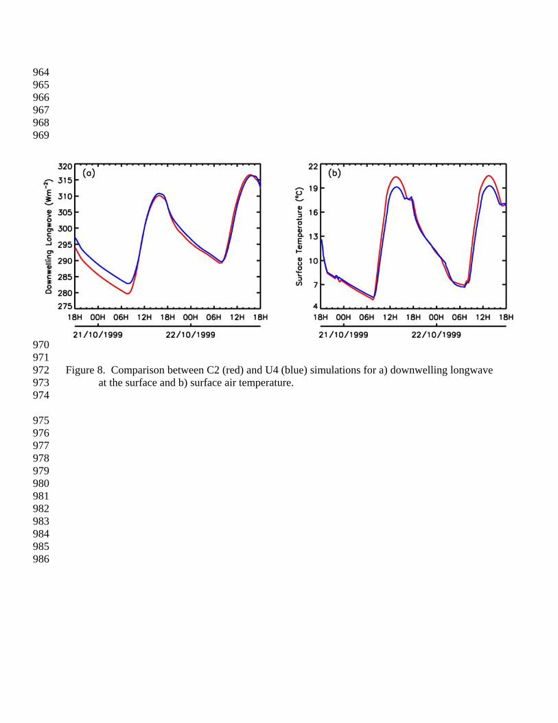
the depth of the soil layer to 70%, referred hereon as C2 and U4 simulations. Differences 510

in downwelling longwave radiation between C2 and U4 (Figure 8a) during the second 511

night are significantly smaller compared to differences found in the C1 and U1 512

simulations (Figure 2b). The decrease in nocturnal radiative forcing occurs in the higher 513

soil moisture situation because the C2 simulation develops a substantially moister 514

boundary layer compared to the U3 simulation during the first day. Enhancement of 515

water vapor in the C2 simulation leads to an increase in downwelling longwave radiation 516

partially offsetting the increase in downwelling longwave radiation in U3 from aerosol 517

loading resulting in a smaller nocturnal SLWRF. Interestingly, comparison of surface air 518

23

temperature between the C2 and U4 simulations show slight nocturnal warming in the U4 519

simulation during parts of the second night (Figure 8b). The reason for this behavior is 520

not understood and illustrates the complex nonlinear interactions exhibited by the NBL 521

dynamics. 522

Of all the experiments considered, the C2 and U4 show the most dramatic change 523

in DTR when compared to C1 (Figure 3). The difference in DTR between C2, U4, and 524

C1 are –7.3 and –8.4°C while the DTR differences between other experiments and C1 are 525

in the range –0.2 to –2°C. When compared to C1, even though the daytime maximum 526

temperature in the C2 and U4 experiments are reduced by more than –5.9°C, the 527

nocturnal minimum temperature is higher in C2 and U4 by more than 1.2°C. The reason 528

for this strong nocturnal warming, despite strong surface air cooling during the daytime, 529

is due to a combination of factors including increased soil heat capacity and bare soil 530

emissivity and an increase in boundary layer moisture during the second day. The impact 531

of enhanced boundary layer moisture in the C2 and U4 experiments is obvious during the 532

second night when the maximum differences in downwelling longwave radiation between 533

both these experiments and C1 exceed 6 W m-2. Christy et al. [2006] found an increasing 534

trend in the nocturnal minimum temperature in irrigated regions of central California and 535

suggested changes in soil heat capacity and enhanced water vapor concentration in the 536

boundary layer as possible reasons. The C2 and U4 experiments in this study do indeed 537

support this hypothesis. 538

The validity of results obtained from the sensitivity analysis for CASES-99 days 539

is further tested in numerical experiments U5 (Pune, 19-21 January 2005) and U6 (Delhi, 540

30 May 2003) where urban land surface characteristics and aerosol optical characteristics 541

24

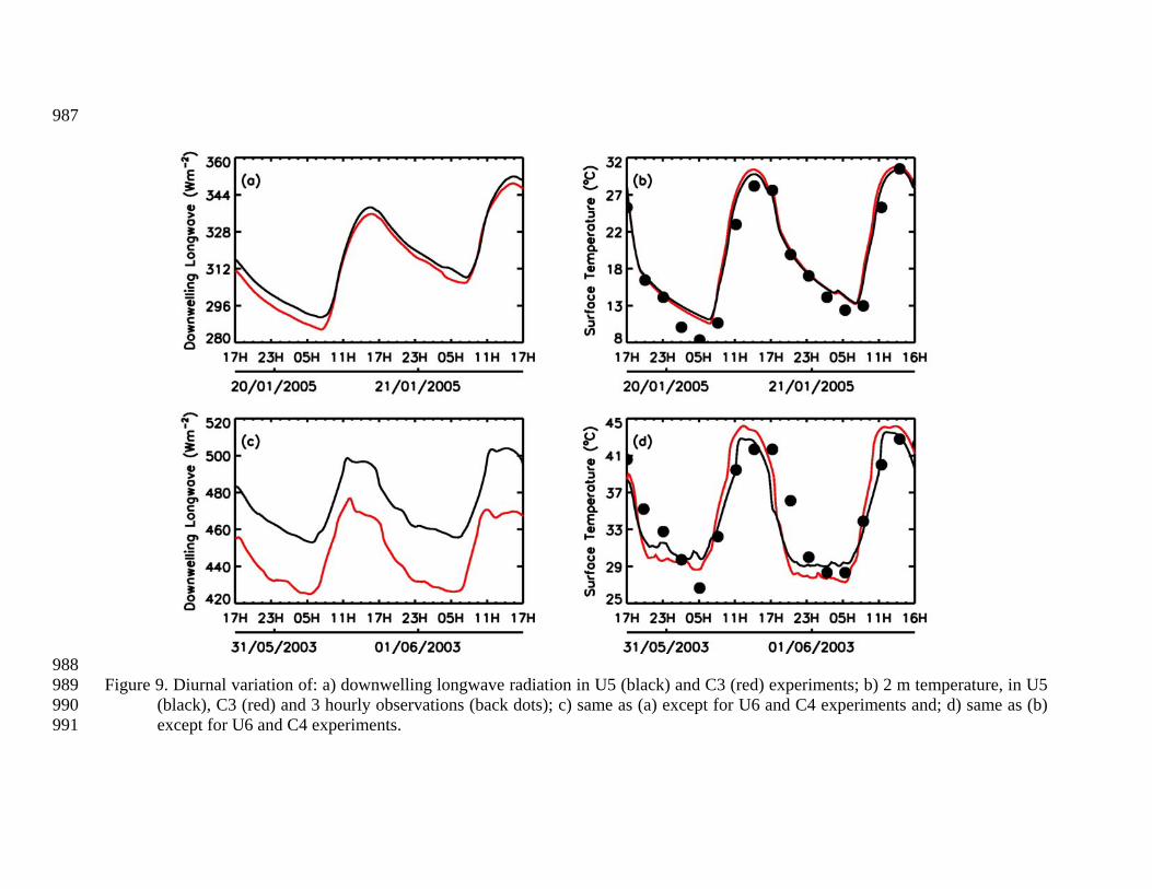
deduced from observations are imposed. For the Pune site, the U5 and C3 experiments 542

show nocturnal SLWRF of ~4.7 W m-2 and 2.7 W m-2 during the first and second night 543

respectively (Figure 9a) which is not substantially different that that found for CASES-99 544

sensitivity analysis. Comparison of the U6 and C4 experiments for the Delhi site show 545

nocturnal SLWRF of 28.5 W m-2 and 29.7 W m-2 during the first and second night 546

respectively (Figure 9c), which is significantly higher than that found in all the other 547

experiments. Note that the higher values of nocturnal SLWRF for the Delhi site is partly 548

due to substantially higher surface temperatures compared to other experiments. The 549

response of 2 m temperature to urban aerosol SLWRF at the Pune site is an increase in 550

nocturnal minimum of 0.51°C and 0.12°C during the first and second nights respectively 551

and a decrease in DTR of 0.72°C (Figure 9b). At the Delhi site, the SLWRF leads to an 552

increase in nocturnal minimum of 1.14 °C and 1.69°C during the first and second nights 553

respectively and a decrease in DTR of 3.07 °C (Figure 9d). Note the experiments were 554

repeated for five other selected days selected for each of the urban sites with similar 555

results. These experiments show that there is considerable variability in the magnitude of 556

nocturnal SLWRF resulting from urban aerosols, compensating for the daytime cooling at 557

the minimum (Figure 9b, Figure 9d) or causing significant nighttime warming on the 558

extreme. 559

Note that the numerical modeling experiments exhibit differing responses of 560

SLWRF and nocturnal warming to variations in aerosol microphysics and composition. 561

The composition and microphysics of aerosols in the U1 experiment are such that it 562

substantially impacts both the downwelling shortwave and longwave radiation. Water 563

soluble aerosols components (nitrates and sulfates) in the U1 experiment, with smaller 564

25

particle size and large number concentrations, lead to significant reduction in daytime 565

downwelling shortwave due to scattering. The soot aerosol component (black carbon) in 566

U1 experiment contributes to absorption in both shortwave and longwave part of the 567

spectrum. In contrast, the coarse mode mineral component with larger particle sizes in 568

the D1 and U6 experiments are substantially more effective absorbers of longwave 569

radiation and leads to higher values of SLWRF that overwhelm the cooling caused the 570

daytime reduction in downwelling shortwave radiation. 571

The numerical experiments considered in this study show a complex response of 572

diurnal surface air temperature variation to urban atmospheric aerosol loading (Figure 3). 573

It is essential to consider aerosol impacts when interpreting surface temperature records 574

in areas such as China, India, and Africa. However, accounting for the aerosol 575

contribution is difficult since the surface air temperature response is dependent on spatial 576

and temporal variations in aerosol concentration, optical characteristics, and is also 577

modulated by other factors such as soil moisture, land surface characteristics, etc. 578

5 Conclusions 579

Aerosol radiative forcing plays an important role on the boundary layer 580

development and surface temperature evolution. In the context of global climate change, 581

there is considerable interest on the role of aerosols in the climate system especially 582

surface temperature. Previous focus of the research effort in this area has been on 583

shortwave radiative forcing with little attention paid to the impact of longwave radiative 584

forcing which may be amplified through nocturnal boundary layer dynamics. Since there 585

is a disproportionate nocturnal contribution to warming trends detected in surface 586

temperature records [Karl et al., 1993], it is important to understand the impact of aerosol 587

26

radiative forcing on nocturnal boundary layer development. This study uses two typical 588

cases of SNBL from the CASES-99 field experiment to examine the impact of urban 589

aerosol radiative forcing on SNBL. For the case study days considered in this study, it is 590

found that: 591

1. Urban aerosols have a nocturnal downwelling longwave radiative forcing impact 592

at the surface similar to that from doubled atmospheric carbon dioxide at local 593

scales. Enhanced nocturnal downwelling longwave from urban aerosols 594

compensate for the daytime cooling due to a reduction in downwelling solar 595

radiation. When diurnal variations in AOD are minimal, urban aerosols maintain 596

the nocturnal minimum surface air temperature the same as that found for clear 597

atmosphere even though the daytime maximum is higher for clear sky conditions. 598

2. Sensitivity of surface air temperature to radiative forcing is higher by a factor of 599

more than three in the NBL compared to CBL since the energy changes impact a 600

shallower layer during the nighttime. 601

3. Aerosol radiative characteristics and diurnal asymmetries in AOD play an 602

important role in determining the overall impact of aerosols on surface air 603

temperature. 604

4. An increase in downwelling longwave radiation at the surface caused by urban 605

aerosols is of sufficient magnitude to cause destabilization of the marginally 606

stable NBL and significant surface air temperature fluctuations from enhanced 607

vertical mixing as suggested by Walters et al. [2007]. 608

5. The impact of urban aerosol longwave radiative forcing is strongly modulated by 609

soil moisture. SLWRF due to urban aerosols decreases for conditions of higher 610

27

soil moisture. This is because with higher soil moisture conditions, the boundary 611

layer water vapor content is enhanced under clear sky conditions, leading to an 612

increase in downwelling longwave at the surface. 613

In order to understand the impact of urban aerosols on surface air temperature and 614

DTR, detailed knowledge regarding diurnal variation of aerosol characteristics including 615

vertical distribution, optical properties, and column loading are needed. Further modeling 616

studies are necessary to examine the impact of aerosol radiative forcing on the marginally 617

stable NBL. Once the NBL conditions most sensitive to urban aerosol radiative forcing 618

are identified, the frequency of occurrence of such conditions needs to be determined 619

from observations. Such analysis will allow quantification of the aerosol radiative forcing 620

contribution to observed nocturnal warming trends. 621

622 Acknowledgements 623

This research was supported by DOE grant DE-FG02-05ER45187 and NSF grant 624

ATM-0417774 Dr. Sundar Christopher was supported by NASA Radiation Sciences 625

Program.626

28

References 627

Allen, G. A., J. Lawrence, and P. Koutrakis (1999), Field validation of a semi-continuous 628

method for aerosol black carbon (aethalometer) and temporal patterns of 629

summertime hourly black carbon measurements in southwestern PA, Atmos. 630

Environ., 33, 817-823, doi:10.1016/S1352-2310(98)00142-3. 631

Balling, R. C., Jr., and R. S. Cerveny (2003), Vertical dimensions of seasonal trends in 632

the diurnal temperature range across the central United States, Geophys. Res. 633

Lett., 30(17), 1878, doi:10.1029/2003GL017776 634

Braganza, K., D.J. Karoly, and J.M. Arblaster (2004a), Diurnal temperature range as an 635

index of global climate change during the 20th century, Geophys. Res. Lett., 31, 636

10.1029/2004GL019998. 637

Braganza, K., D.J. Karoly, A.C. Hirst, A.C. Hirst, P. Stott, R.J. Stouffer, and S.F.B. Tett 638

(2004b) Simple indices of global climate variability and change: Part II - 639

Attribution of climate change during the 20th century, Climate Dyn., 22, 823-838, 640

10.1007/s00382-004-0413-1. 641

Chen, C., and W. R. Cotton (1983), A one-dimensional simulation of the stratocumulus-642

capped mixed layer, Boundary-Layer Meteorol., 25, 289-321, DOI: 643

10.1007/BF00119541. 644

Chen, F., K.W. Manning, S.B. LeMone, J.G. Alfieri, R. Roberts, M. Tewari, D. Niyogi, 645

T.W. Horst, S.P. Oncley, J. Basara, P.D. Blanken (2007), Description of 646

Evaluation of the Characteristics of the NCAR High-Resolution Land Data 647

Assimilation System During IHOP-02. J. Appl. Meteorol., 46, 694-713, DOI: 648

10.1175/JAM2463.1. 649

29

Christopher, S.A., J. Wang, Q. Ji, and S-C. Tsay (2003), Estimation of shortwave dust 650

aerosol radiative forcing during PRIDE, J. Geophys. Res., 108(D19), 8956, 651

doi:10.1029/2002JD002787. 652

Christy, J. R., W. B. Norris, K. Redmond, and K. P. Gallo (2006), Methodology and 653

results of calculating central California surface temperature trends: Evidence of 654

human-induced climate change? J. Climate, 19, 548-563, DOI: 655

10.1175/JCLI3627.1. 656

Cotton, W. R., R. A. Pielke, R. L. Walko, G. E. Liston, and C. J. Tremback (2003), 657

RAMS 2001: Current status and future directions, Meteorol. Atmos. Phys., 82, 5-658

29, 10.1007/s00703-001-0584-9. 659

Dai, A., and K. E. Trenberth (2004), The diurnal cycle of its depiction in the Community 660

Climate System Model, J. Climate, 17, 930-951. 661

Dai, A., Kevin E. Trenberth, and T. R. Karl (1999), Effects of clouds, soil moisture, 662

precipitation, and water vapor temperature range, J. Climatol., 12, 2451-2473, 663

DOI: 10.1175/1520-0442(2004)017<0930:TDCAID>2.0.CO;2. 664

Dorsey, J. R., E. Nemitz, M. W. Gallagher, D. Fowler, P. I. Williams, K. N. Bower, and 665

K. M. Beswick (2002), Direct measurements and parameterisation of aerosol flux, 666

concentration and emission velocity above a city, Atmos. Environ., 36, 791-800, 667

doi:10.1016/S1352-2310(01)00526-X. 668

Estournel, C., R. Vehil, D. Guedalia, J. Fontan, and A. Druilhet (1983), Observations and 669

modeling of downward radiative fluxes (solar and infrared) in urban/rural areas, J. 670

Climate Appl. Meteorol., 22, 134-142, DOI: 10.1175/1520-671

0450(1983)022<0134:OAMODR>2.0.CO;2. 672

30

Fu, Q., and K. N. Liou (1992), On the correlated k-distribution method for radiative 673

transfer in nonhomogeneous atmospheres, J. Atmos. Sci., 49, 2139-2156, DOI: 674

10.1175/1520-0469(1992)049<2139:OTCDMF>2.0.CO;2. 675

—— (1993) Parameterization of the radiative properties of cirrus clouds, J. Atmos. Sci., 676

50, 2008-2025, DOI: 10.1175/1520-0469(1993)050<2008:POTRPO>2.0.CO;2. 677

Garratt, J. R., A. B. Pittock, and K. Walsh (1990), Response of the atmospheric boundary 678

layer and soil layer to a high altitude, dense aerosol cover, J. Appl. Meteorol., 29, 679

35-52, DOI: 10.1175/1520-0450(1990)029<0035:ROTABL>2.0.CO;2. 680

Guasta, M. D. (2002), Daily cycles in urban aerosols observed in Florence (Italy) by 681

means of an automatic 532-1064nm LIDAR, Atmos. Environ., 36, 2853-2865, 682

10.1016/S1352-2310(02)00136-X. 683

Hansen, J., M. Sato, and R. Ruedy (1995), Long-term changes of the diurnal temperature 684

cycle: Implications about mechanisms of global climate change, Atmos. Res., 37, 685

175-210, doi:10.1016/0169-8095(94)00077-Q. 686

Harrington, J. Y., T. Reisin, W. R. Cotton, and S. M. Kreidenweis (1999), Cloud 687

resolving simulations of Arctic stratus: Part II: Transition-season clouds, Atmos. 688

Res., 51, 45-75, doi:10.1016/S0169-8095(98)00098-2. 689

Hess, M., P. Koepke, and I. Schult (1998), Optical properties of aerosols and clouds: The 690

software package OPAC, Bull. Am. Meteorol. Soc., 79, 831-844, DOI: 691

10.1175/1520-0477(1998)079<0831:OPOAAC>2.0.CO;2. 692

IPCC (2007), Climate Change 2007 - The Physical Science Basis: Working Group I 693

Contribution to the Fourth Assessment Report of the IPCC (Climate Change 694

2007). Solomon, S., D. Qin, M. Manning, Z. Chen, M. Marquis, K.B. Averyt, M. 695

31

Tignor and H.L. Miller (eds.), Cambridge University Press, Cambridge, United 696

Kingdom and New York, NY, USA. 697

Jacobson, M. Z. (1997), Development and application of a new air pollution modeling 698

system -- Part III. Aerosol-phase simulations, Atmos. Environ., 31, 587-608, 699

doi:10.1016/S1352-2310(96)00201-4. 700

Kalnay, E., and M. Cai (2003), Impact of urbanization and land-use change on climate, 701

Nature, 423, 528-531. 702

Karl, T. R., G. Kukla, and J. Gavin (1984), Decreasing diurnal temperature range in the 703

United States and Canada from 1941 through 1980, J. Climatol., 23, 1489-1503, 704

DOI: 10.1175/1520-0450(1984)023<1489:DDTRIT>2.0.CO;2. 705

Karl, T. R., P. D. Jones, R. W. Knight, G. Kukla, N. Plummer, V. Razuvayev, K. P. 706

Gallo, J. Lindseay, R. J. Charlson, and T. C. Peterson (1993), A new perspective 707

on recent global warming: asymmetric trends of daily maximum and minimum 708

temperature, Bull. Am. Meteorol. Soc, 74, 1007-1023, DOI: 10.1175/1520-709

0477(1993)074<1007:ANPORG>2.0.CO;2. 710

Koch, D., T. C. Bond, D. Streets, N. Unger, and G. R. v. d. Werf (2007), Global impacts 711

of aerosols from particular source regions and sectors, J. Geophys. Res., 112, 712

D02205, doi:10.1029/2005JD007024. 713

Mahrer, Y., and R. A. Pielke (1977), The effects of topography on sea and land breezes in 714

a two-dimensional numerical model, Mon. Weather Rev., 105, 1151-1162, DOI: 715

10.1175/1520-0493(1977)105<1151:TEOTOS>2.0.CO;2. 716

32

Makowski, K., M. Wild, and A. Ohmura (2008), Diurnal temperature range over Europe 717

between 1950 and 2005, Atmos. Chem. Phys. Discuss., 8, 7051-7084, 718

www.atmos-chem-phys.net/8/6483/2008/. 719

Mårtensson, E. M., E. D. Nilsson, G. Buzorius, and C. Johansson (2006), Eddy 720

covariance measurements and parameterisation of traffic related particle 721

emissions in an urban environment, Atmos. Chem. Phys., 6, 769-785, www.atmos-722

chem-phys.net/6/769/2006/. 723

Pandithurai, G., R. T. Pinker, P. C. S. Devara, T. Takamura, and K. K. Dani (2007), 724

Seasonal asymmetry in diurnal variation of aerosol optical characteristics over 725

Pune, western India, J. Geophys. Res., 112, D08208, doi:10.1029/2006JD007803. 726

Panicker, A. S., G. Pandithurai, P. D. Safai, and S. Kewat (2008), Observations of 727

enhanced aerosol longwave radiative forcing over an urban environment, 728

Geophys. Res. Lett., 35, L04817, doi:10.1029/2007GL032879 729

Pielke, R. A., and T. Matsui (2005), Should light wind and windy nights have the same 730

temperature trends at individual levels even if the boundary layer averaged heat 731

content change is the same? Geophys. Res. Lett., 32, L21813, 732

10.1029/2005GL024407. 733

Pielke Sr., R.A., C. Davey, D. Niyogi, S. Fall, J. Steinweg-Woods, K. Hubbard, Lin, M. 734

Cai, Y.-K. Lim, H. Li, J. Nielsen-Gammon, K. Gallo, R. Hale, R. Mahmood, S. 735

Foster, R. T. McNider, and P. Blanken (2007), Unresolved issues with the 736

assessment of multi-decadal global land temperature trends, J. Geophys. Res. 112, 737

D24S08, doi:10.1029/2008JD008229. 738

33

Poulos, G. S., W. Blumen, D. C. Fritts, J. K. Lundquist, J. Sun, S. P. Burns, C. Nappo, R. 739

Banta, R. Newsom, J. Cuxart, E. Terradellas, B. Balsley, and M. Jensen (2002), 740

CASES-99: A comprehensive investigation of the stable nocturnal boundary 741

layer, Bull. Am. Meteorol. Soc., 83, 555-581, DOI: 10.1175/1520-742

0477(2002)083<0555:CACIOT>2.3.CO;2. 743

Ramanathan, V., P. J. Crutzen, J. T. Kiehl and D. Rosenfeld, (2001a), Aerosols, climate, 744

and the hydrological cycle, Science, 294, 2119-2124. 745

Ramanathan, V., P. J. Crutzen, J. Lelieveld, A. P. Mitra, D. Althause, J. Anderson, M. P. 746

O. Andreae, W. Cantrell, C.R. Cass, C.E. Chung, A.D. Clarke, J.A. Coakley, 747

W.D. Collins, W.C. Conant, F. Dulac, J. Heintzenberg, B. Holben, S. Howell, J. 748

Hudson, A. Jayaraman, J.T. Kiehl, T.N. Krishnamurti, D. Lubin, G. McFarquhar, 749

T. Novakov, J.A. Ogren, I.A. Podgorny, K. Prather, K. Priestley, J.M. Prospero, 750

P.K. Quinn, K. Rajeev, P. Rasch, S. Rupert, R. Sadourny, S.K. Satheesh, G.E. 751

Shaw, P. Sheridan, and F.P.J. Valero (2001b), Indian Ocean Experiment: An 752

integrated analysis of the climate forcing and effects of the great Indo-Asian haze, 753

J. Geophys. Res., 106(D22), 28,371–28,398. 754

Singh, S., S. Nath, R. Kohli, and R. Singh, (2005), Aerosols over Delhi during pre-755

monsoon months: Characteristics and effects on surface radiation forcing, 756

Geophys. Res. Lett., 32, L13808, doi:10.1029/2005GL023062. 757

Smirnov, A., B. N. Holben, T. F. Eck, I. Slutsker, B. Chatenet, and R. T. Pinker (2002), 758

Diurnal variability of aerosol optical depth observed at AERONET (Aerosol 759

Robotic Network) sites, Geophys. Res. Lett., 29(23), 2115, 760

doi:10.1029/2002GL016305. 761

34

Steeneveld, G. J., B. Wiel, and A. A. M. Holstag (2006), Modeling the evolution of the 762

atmospheric boundary layer coupled to the land surface for three contrasting 763

nights in CASES-99, J. Atmos. Sci., 63, 920-935, DOI: 10.1175/JAS3654.1. 764

Stone, D. A., and A. J. Weaver (2003), Factors contributing to diurnal temperature range 765

trends in twentieth and twenty-first century simulations of the CCCma coupled 766

model, Climate Dyn., 20, 435–445. 767

Venkatram, A., and R. Viskanta (1977), Radiative effects of elevated pollutant layers, J. 768

Appl. Meteorol., 16, 1256-1272, DOI: 10.1175/1520-769

0450(1977)016<1256:REOEPL>2.0.CO;2. 770

Walko, R. L., L. E. Band, J. Baron, T. G. F. Kittel, R. Lammers, T. J. Lee, D. Ojima, R. 771

A. Pielke, C. Taylor, C. Tague, C. J. Tremback, and P. L. Vidale (2000), Coupled 772

atmosphere-biophysics-hydrology models for environmental modeling, J. Appl. 773

Meteorol., 39, 931-944, DOI: 10.1175/1520-774

0450(2000)039<0931:CABHMF>2.0.CO;2. 775

Walters, J. T., R. T. McNider, X. Shi, W. B. Norris, and J. R. Christy (2007), Positive 776

surface temperature feedback in the stable nocturnal boundary layer, Geophys. 777

Res. Lett., 34, L12709, doi:10.1029/2007GL029505. 778

Wang, J., and S. A. Christopher (2006), Mesoscale modeling of Central American smoke 779

transport to the United States: 2. Smoke radiative impact on regional surface 780

energy budget and boundary layer evolution, J. Geophys. Res., 111, D14S92, 781

doi:10.1029/2005JD006720. 782

Wang, J., S. A. Christopher, U. S. Nair, J. S. Reid, E. M. Prins, J. Szaykman, and J. L. 783

Hand (2006), Mesoscale modeling of Central American smoke transport to the 784

35

United States: 1. "Top-down" assessment of emission strength and diurnal 785

variation impacts, J. Geophys. Res., 111, D05S17, doi:10.1029/2005JD006416. 786

Welch, R., and W. Zdunkowski (1976), A radiation model of the polluted atmospheric 787

boundary layer, J. Atmos. Sci., 33, 2170-2184, DOI: 10.1175/1520-788

0469(1976)033<2170:ARMOTP>2.0.CO;2. 789

Yu, H., S. C. Liu, and R. E. Dickinson (2002), Radiative effects of aerosols on the 790

evolution of the atmospheric boundary layer, J. Geophys. Res., 107(D12), 4142, 791

doi:10.1029/2001JD000754. 792

Zdunkowski, W. G., R. M. Welch, and J. Paegle (1976), One-dimensional numerical 793

simulation of the effects of air pollution on the planetary boundary layer, J. 794

Atmos. Sci., 33, 2399-2414, DOI: 10.1175/1520-0469(1976)033. 795

Zhou, L., R. E. Dickinson, Y. Tian, R. S. Vose, and Y. Dai (2007), Impact of vegetation 796

removal and soil aridation on diurnal temperature range in a semiarid region: 797

Application to the Sahel, Proc. Natl. Acad. Sci., 104, 17937-17942, doi: 798

10.1073/pnas.0700290104. 799

Zobler, L. (1999), Global Soil Types, 1-Degree Grid (Zobler). Data set. Available on-line 800

[http://www.daac.ornl.gov] from Oak Ridge National Laboratory Distributed 801

Active Archive Center, Oak Ridge, Tennessee, U.S.A. 802

doi:10.3334/ORNLDAAC/418. 803

804

36

Figure Legends 805

Figure 1. Comparison between observations (black line) and C1 simulation (red line) of: 806

a) downwelling shortwave; b) downwelling longwave; c) upwelling longwave; d) 807

sensible heat flux; e) latent heat flux; f) surface air temperature; and g) relative 808

humidity. 809

Figure 2. Comparison between C1 (red), D1 (green), U1 (blue), and X2 (black) 810

simulations. a) downwelling shortwave; b) downwelling longwave; c) surface air 811

temperature; and c) upwelling longwave. 812

Figure 3. Diurnal temperature range (open triangle), maximum (solid square) and 813

minimum (open circle) temperatures for the different experiments. The values are 814

valid for the time period including the first day and the second night. 815

Figure 4. Comparison between C1 (red) and U2 (blue) simulations for a) downwelling 816

longwave at the surface and b) surface air temperature. 817

Figure 5. Comparison between C1 (red) and U3 (blue) simulations for a) downwelling 818

longwave at the surface and b) surface air temperature. 819

Figure 6. Diurnal variation of aerosol extinction coefficient in the infrared (10.2-12.5 820

μm) in the U1 experiment at the first model level (solid line) and averaged for the 821

atmospheric column in the lowest 100 m. 822

Figure 7. Bifurcation diagrams with enhanced downward radiation from aerosols as the 823

bifurcation parameter (x axis) and boundary layer potential temperature as the 824

response variable (y axis) plotted along the x axis and the boundary layer 825

potential temperature. Line colors give roughness length: green – z0=0.1 m, red – 826

z0 = 0.25 m, pink - z0 = 0.5 m, blue - z0 = 1.0 m. (a) Bifurcation diagram for a 827

37

geostrophic wind speed of 3 m s-1. (b) Bifurcation diagram for a geostrophic 828

wind speed of 7 m s-1. (c) Bifurcation diagram for a geostrophic wind speed of 10 829

m s-1. 830

Figure 8. Comparison between C2 (red) and U4 (blue) simulations for a) downwelling 831

longwave at the surface and b) surface air temperature. 832

Figure 9. Diurnal variation of: a) downwelling longwave radiation in U5 (black) and C3 833

(red) experiments; b) 2 m temperature, in U5 (black), C3 (red) and 3 hourly 834

observations (back dots); c) same as (a) except for U6 and C4 experiments and; d) 835

same as (b) except for U6 and C4 experiments. 836

837

38

TABLES 838 839 840

Aerosol Model

Composition 0.55 μm AOD (80%

relative humidity) Component Number Density (cm-3)

Mode radius (μm)

Urban Water Soluble 28,000 0.0212

0.643 Insoluble 1.5 0.471 Soot 130,000 0.0118

Urban [Panicker et al.

2008]

Water Soluble 0.0212 0.347 Insoluble 0.471

Soot 0.0118

Urban [Singh et al. 2005]

Soot 130,000 0.0118

0.863

Water Soluble 10,000 0.0212 Mineral,

Nucleation Mode 269.5 0.07

Mineral, Accumulation

Mode 5.050 0.39

Mineral, Coarse Mode 3.850 1.90

Desert

Water Soluble 0.018 0.0212

0.286

Mineral, Nucleation mode 0.033 0.07

Mineral, Accumulation

mode 0.747 0.39

Mineral, Coarse mode 0.202 1.90

841 Table 1. Composition of aerosol models used in the study. Lognormal distribution is 842 assumed for aerosol model components whose subcomponents are as follows: Water 843 Soluble: Mixture of sulfates, nitrates and organics; Insoluble: Mixture of soil particles 844 and organic material; Soot: Black carbon; Mineral: Mixture of quartz and clay [Hess et 845 al., 1998]. 846 847 848 849 850 851 852 853 854 855

39

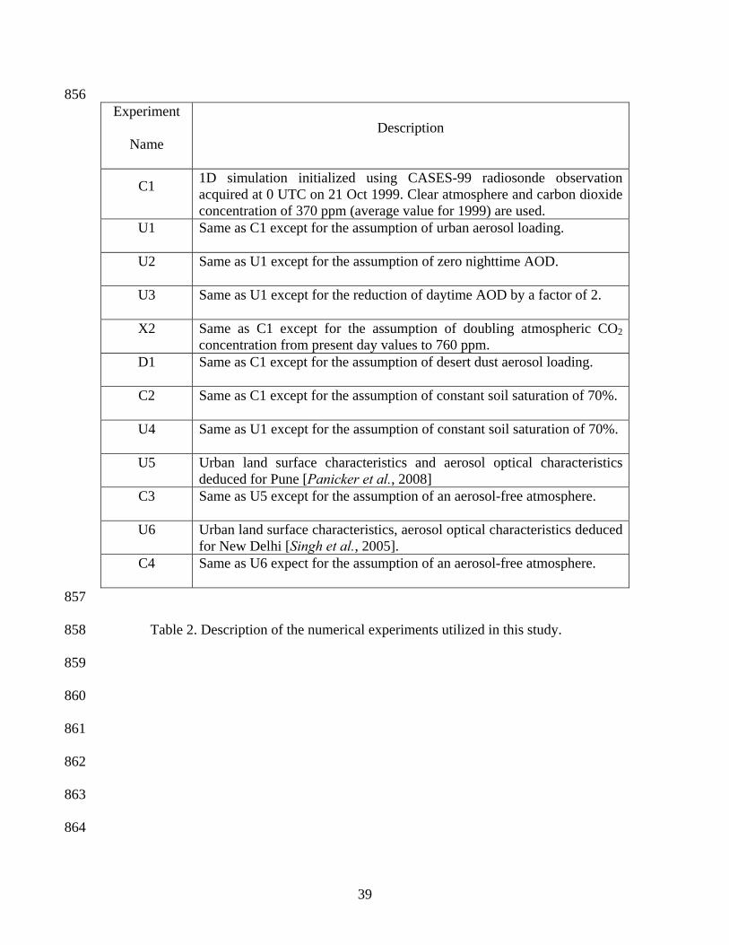
856 Experiment

Name Description

C1 1D simulation initialized using CASES-99 radiosonde observation acquired at 0 UTC on 21 Oct 1999. Clear atmosphere and carbon dioxide concentration of 370 ppm (average value for 1999) are used.

U1 Same as C1 except for the assumption of urban aerosol loading.

U2 Same as U1 except for the assumption of zero nighttime AOD.

U3 Same as U1 except for the reduction of daytime AOD by a factor of 2.

X2 Same as C1 except for the assumption of doubling atmospheric CO2 concentration from present day values to 760 ppm.

D1 Same as C1 except for the assumption of desert dust aerosol loading.

C2 Same as C1 except for the assumption of constant soil saturation of 70%.

U4 Same as U1 except for the assumption of constant soil saturation of 70%.

U5 Urban land surface characteristics and aerosol optical characteristics deduced for Pune [Panicker et al., 2008]

C3 Same as U5 except for the assumption of an aerosol-free atmosphere.

U6 Urban land surface characteristics, aerosol optical characteristics deduced for New Delhi [Singh et al., 2005].

C4 Same as U6 expect for the assumption of an aerosol-free atmosphere.

857

Table 2. Description of the numerical experiments utilized in this study. 858

859

860

861

862

863

864

40

865

866

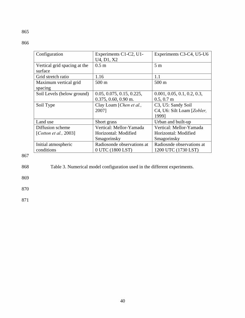
Configuration Experiments C1-C2, U1-U4, D1, X2

Experiments C3-C4, U5-U6

Vertical grid spacing at the surface

0.5 m 5 m

Grid stretch ratio 1.16 1.1 Maximum vertical grid spacing

500 m 500 m

Soil Levels (below ground) 0.05, 0.075, 0.15, 0.225, 0.375, 0.60, 0.90 m.

0.001, 0.05, 0.1, 0.2, 0.3, 0.5, 0.7 m

Soil Type Clay Loam [Chen et al., 2007]

C3, U5: Sandy Soil C4, U6: Silt Loam [Zobler, 1999]

Land use Short grass Urban and built-up Diffusion scheme [Cotton et al., 2003]

Vertical: Mellor-Yamada Horizontal: Modified Smagorinsky

Vertical: Mellor-Yamada Horizontal: Modified Smagorinsky

Initial atmospheric conditions

Radiosonde observations at 0 UTC (1800 LST)

Radiosnde observations at 1200 UTC (1730 LST)

867

Table 3. Numerical model configuration used in the different experiments. 868

869

870

871

41

872 Figure 1. Comparison between observations (black line) and C1 simulation (red line) of: 873

a) downwelling shortwave; b) downwelling longwave; c) upwelling longwave; d) 874 sensible heat flux; e) latent heat flux; f) surface air temperature; and g) relative 875 humidity. 876

42

877 878 Figure 2. Comparison between C1 (red), D1 (green), U1 (blue), and X2 (black) simulations. a) downwelling shortwave; b) 879

downwelling longwave; c) surface air temperature; and c) upwelling longwave. Note than in panel a, the differences between 880 C1 and X2 are negligible and thus the curve for C1 (red) is hidden by the one for X2. 881

882

43

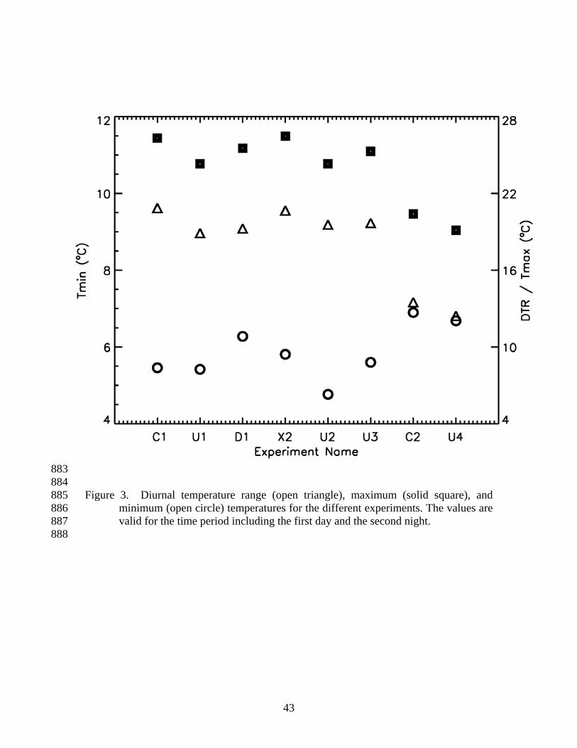
883 884 Figure 3. Diurnal temperature range (open triangle), maximum (solid square), and 885

minimum (open circle) temperatures for the different experiments. The values are 886 valid for the time period including the first day and the second night. 887

888

44

889 890 891 892 893 894 895

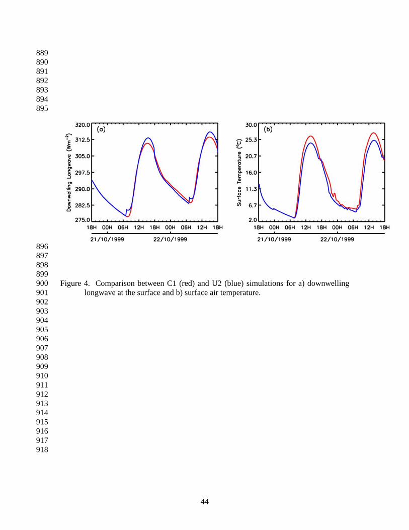
896 897 898 899 Figure 4. Comparison between C1 (red) and U2 (blue) simulations for a) downwelling 900

longwave at the surface and b) surface air temperature. 901 902 903 904 905 906 907 908 909 910 911 912 913 914 915 916 917 918

45

919 920 921 922 923 924

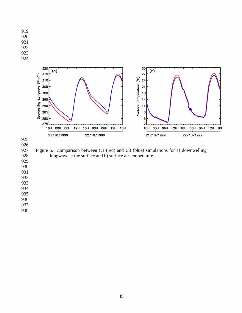
925 926 Figure 5. Comparison between C1 (red) and U3 (blue) simulations for a) downwelling 927

longwave at the surface and b) surface air temperature. 928 929 930 931 932 933 934 935 936 937 938

46

939 940 941 942 943 944

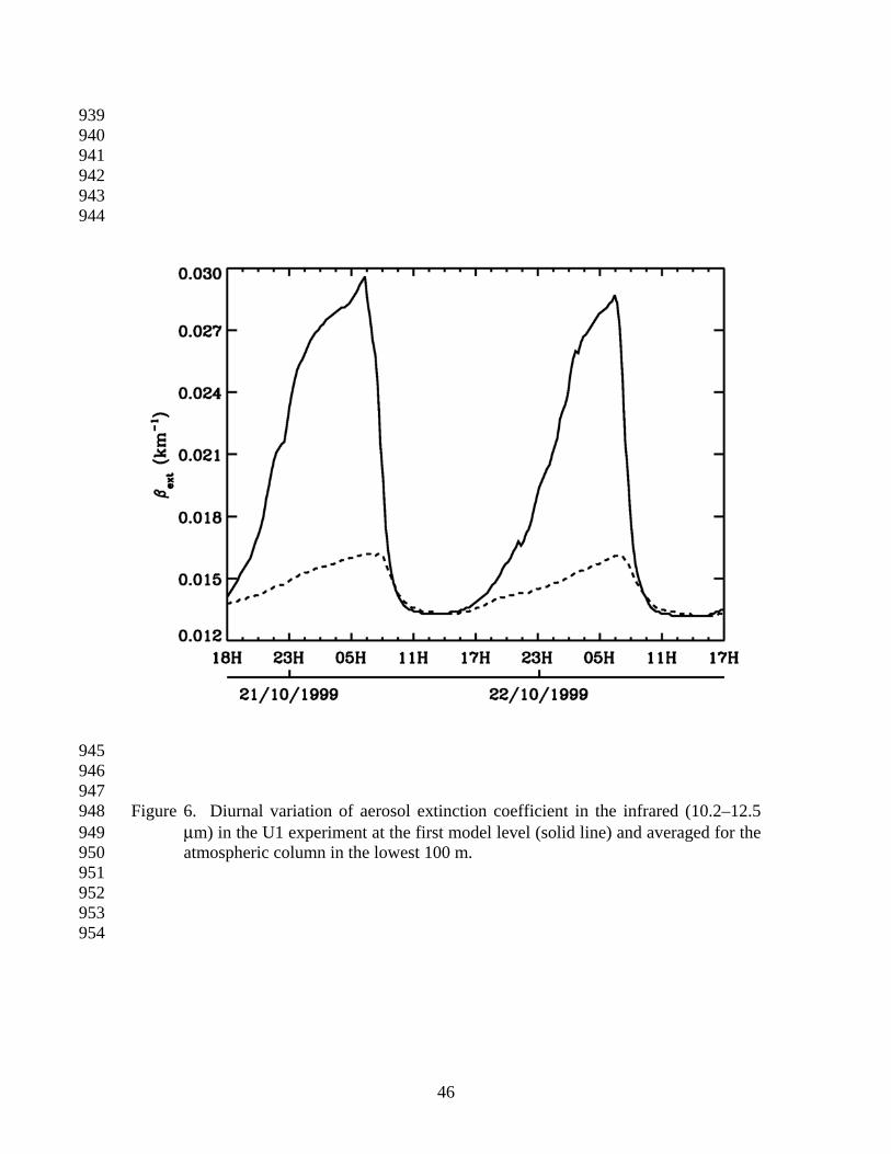
945 946 947 Figure 6. Diurnal variation of aerosol extinction coefficient in the infrared (10.2–12.5 948

μm) in the U1 experiment at the first model level (solid line) and averaged for the 949 atmospheric column in the lowest 100 m. 950

951 952 953 954

47

955

956 Figure 7. Bifurcation diagrams with enhanced downward radiation from aerosols as the 957 bifurcation parameter (x axis) and boundary layer potential temperature as the response 958 variable (y axis) plotted along the x axis and the boundary layer potential temperature. 959 Line colors give roughness length: green – z0=0.1 m, red – z0 = 0.25 m, pink - z0 = 0.5 960 m, blue - z0 = 1.0 m. (a) Bifurcation diagram for a geostrophic wind speed of 3 m s-1. (b) 961 Bifurcation diagram for a geostrophic wind speed of 7 m s-1. (c) Bifurcation diagram for a 962 geostrophic wind speed of 10 m s-1. 963

964 965 966 967 968 969

970 971 Figure 8. Comparison between C2 (red) and U4 (blue) simulations for a) downwelling longwave 972

at the surface and b) surface air temperature. 973 974

975 976 977 978 979 980 981 982 983 984 985 986

987

988 Figure 9. Diurnal variation of: a) downwelling longwave radiation in U5 (black) and C3 (red) experiments; b) 2 m temperature, in U5 989

(black), C3 (red) and 3 hourly observations (back dots); c) same as (a) except for U6 and C4 experiments and; d) same as (b) 990 except for U6 and C4 experiments. 991