SEGMENTAL Box GIRDER: DEFLECTION

PROBABILITY AND BAYESIAN UPDATING

By Zdenek P. Baiant/ Fellow, ASCE, and Joong-Koo Kim2

ABSTRACT: Probabilistic prediction of the confidence limits on long-time deflec­tions and internal forces of prestressed concrete segmental box-girder bridges is developed. The uncertainty of the predictions based on the existing models for concrete creep (the prior) is very large, but it can be greatly reduced by Bayesian updating on the basis of short-time measurements of the deflections during con­struction or of short-time creep and shrinkage strains of specimens made from the same concrete as the bridge. The updated (posterior) probabilities can be obtained by latin hypercube sampling, which reduces the problem to a series of deterministic creep structural analyses for randomly generated samples of random parameters of the creep and shrinkage prediction model. The method does not require lineariza­tion of the problem with regard to the random parameters, and a large number of the random parameters can be taken into account. Application to a typical box­girder bridge with age differences between its segments and with a change of struc­tural system from statically indeterminate to determinate is illustrated numerically. The results prove that design for extreme, rather than mean, long-time deflections and internal forces is feasible. Adoption of such a design approach would improve long-term serviceability of box-girder bridges.

INTRODUCTION

Prestressed concrete segmental box-girder bridges are structures that are particularly sensitive to their long-time deformations. Deflections much in excess of their calculated values or severe cracking after a longer service period have often been experienced. The consequences, which include costly repairs and even closing of a bridge before the end of its design lifetime, represent a great economic loss. One important cause of this situation is no doubt the fact that, outside the laboratory, creep and shrinkage of concrete are highly uncertain random phenomena, influenced by many random pa­rameters. Predicting only mean deflections, which is the current practice, is insufficient. The design should be based on predictions of extreme deflec­tions that are exceeded with a certain specified small probability.

The probabilistic approach necessitates a realistic creep prediction model, such as the BP model (Bazant and Panula 1978,1980, 1982). In probabilistic analysis, it would make little sense to use simple but unrealistic models that have large systematic errors resulting from inadequacy of the mathematical model per se, rather than from randomness of influencing parameters. On the other hand, the usefulness of a sophisticated creep prediction model, such as the BP model, is limited unless its use is combined with a probabilistic approach.

'Prof. ofCiv. Engrg., Dept. ofCiv. Engrg., The Tech. Inst., Northwestern Univ., Evanston, IL 60208.

2Grad. Res. Asst., Dept. of Civ. Engrg., The Tech. Inst., Northwestern Univ., Evanston, IL.

Note. Discussion open until March I, 1990. To extend the closing date one mon~h, a written request must be filed with the ASCE Manager of Journals. The manuscnpt for this paper was submitted for review and possible publi~ation on June 7, 1988. This paper is part of the Journal of Structural Engmeenng, Vol. 115, No. 10, October, 1989. ©ASCE, ISSN 0733-9445/89/0010-2528/$1.00 + $.15 per page. Paper No. 23976.

2528

If creep and shrinkage properties of concrete are predicted solely on the basis of the existing models, the uncertainty is very large. For the BP model (Bazant and Panula 1978, 1980, 1982), errors that are exceeded with a 5% probability (2.5% on the plus side, 2.5% on the minus side) are about 37%, while for the simpler but less realistic models of ACI Committee 209/11 (1971, 1982) and CEB-FIP (1978) they are 75% and 91%, respectively (BaZant and Panula 1982; BaZant 1988; Zebich and BaZant 1981). As shown in BaZant and Panula (1982), this uncertainty can be greatly reduced if some short­time measurements are made and Bayesian statistical reasoning applied. An analytical method to do that for long-time creep compliance of concrete was developed in Bazant (1983) and Bazant and Chern (1984). This method, however, works only if the creep law is linearized and if there are only few random parameters (two or three). None of these simplifications is adequate for predicting deflections of an entire box girder.

General applicability can be achieved by combining Bayesian updating with a sampling approach, as formulated in Bazant (1985). This reduces the problem to a series of conventional (deterministic) structural creep analyses for various samples of random parameters. A novel sampling method, called latin hypercube sampling (McKay 1980; McKay et a1. 1979, 1976), has been adopted. This sampling method, which was originally applied to direct (non­Bayesian) probabilistic prediction of structural creep effects (Bazant and Liu 1985), and was later extended to Bayesian extrapolation of shrinkage data (Bazant et a1. 1987), is computationally much more efficient than the method of point estimates used previously (Madsen and Bazant 1983).

In the present study, Bazant's (1985) method used for shrinkage in Bazant et a1. (1987) will be applied to short-time measurements during construction in order to improve the predictions of long-time deflections and internal forces in a segmental box girder which undergoes a change of its structural system during construction and has a nonuniform age of concrete. This approach has the potential of substantially reducing the uncertainty of long-time pre­dictions and making it possible to adjust the vertical alignment of the seg­ments during construction, thereby minimizing deviations from the desired vertical profile of the bridge.

LINEAR CREEP ANALYSIS OF SEGMENTAL Box GIRDER

Concrete is assumed to behave as an aging linearly viscoelastic material (Bazant 1982a, 1988). It is characterized by the compliance function J(t, t') representing the strain of concrete at time t caused by a unit uniaxial stress applied at time t'. J(t, t') is defined, according to the BP model (Bazant and Panula 1978, 1980, 1982), as a sum of the asymptotic elastic compliance, the basic creep compliance, and the drying creep compliance. The shrinkage strain, also defined according to the BP model, is assumed to occur ho­mogeneously throughout the cross section, which is a usual simplification in design. The thermal strains are ignored.

In a typical segmental bridge (Fig. 1), the age of concrete is nonuniform. Let time t represent the age of the oldest segment, numbered k = I. The compliance function of segment number k is denoted as Jk(t, t'). If the prop­erties of concrete are the same as in the segment number 1, then Jk(t,t') = JI(t - Ilb t' - Ilk) = compliance function of segment number I, where Ilk is the age difference between the segments k and 1.

2529

b)

c)

492

~ ,. TYPICAL SECTION

d)~r~I' '" .., .- ON PIER

~-~~~~~ I---- 249 -..I

e)

.110 .117

"I

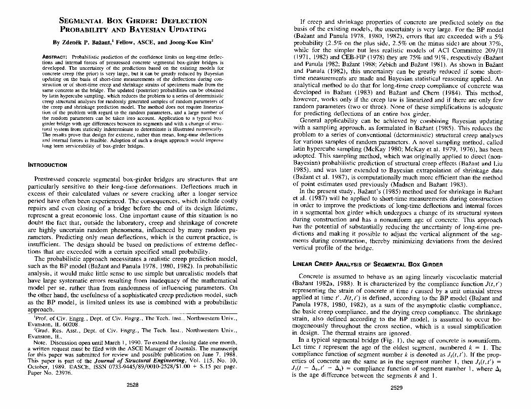
FIG. 1. Bridge Analyzed in Example (Kishwaukee River Bridge, III.): (a) Longi­tudinal Cross Section; (b) Cantilever (Half-Span) Analyzed; (c) Box Girder Seg­ment; (d) Cross Section Simplified for Analysis; and (e) Elastic Deflection Curve and Deflections Measured (Dimensions in Inches, 1 in. = 25.4 mm)

For numerical computation, time t is subdivided by discrete times tj (i =

1,2 ... ) in time steps I1tj = tj - t j _ l • Until time tm the box girder consists of a statically determinate cantilever, and the stress is then constant if the load is constant. We assume that the load due to the own weight of the segment number k is applied instantly at time tk at which this segment is placed in position and prestressed (or freed from the formwork, if cast in situ). Thus, all the stresses vary at t = tk by a sudden jump and subsequently remain constant until time tHI when the next segment is placed. This results in a staircase history of moment (Fig. 2). At time tm the cantilevers are

2530

1200

:; 600

E-< Z ~

::::s a ::::!! 400

-- MINIMUM MOMENT (ON PIER) - - - MAXIMUM MOMENT (AT MIDSPAN)

r-I/-~-------

Og~0----------10rO==~-----ITI0----~r----2T~0---------J'6-0-

DAYS

FIG. 2. History of Minimum Bending Moment at Support and Maximum Bending Moment at Midspan Produced by Construction Sequence with Time Steps Con­sidered in Analysis

joined, and afterwards the stresses gradually redistribute due to statical in­determinacy. This causes, after time tm , the stresses to vary continuously in time .

For our purposes the box-girder bridge (Fig. 1) may be analyzed as a beam in which the cross sections remain plane and normal. We neglect the shear lag (Kffstek and Bazant 1987), for the sake of simplicity. We ignore the effects of nonprestressed steel, and of transverse or vertical prestressing (if any). Perfect bond is assumed for the tendons. For the sake of simplicity, we assume that the two cantilevers joined at midspan are symmetric, and the ages of symmetric segments are the same (Fig. 3). The supports are assumed to prevent rotation but permit free horizontal dilatation of the span.

The cantilevers are made continuous at time tm • Since rotations at the can­tilever ends are impossible after time (m, a redundant bending moment, X, gradually builds up at the midspan after time tm • Due to symmetry, however, the shear force at midspan is zero, so the structure is only singly redundant (Fig. 3).

The structure is analyzed with a computer program for the layered finite element method. Each segment of the box girder (Fig. 1) represents one finite element, which is subdivided into layers. The reinforcement represents additional elastic layers. The prestressing is implemented by introducing for the prestressed bars initial strains for treatment of creep, and the constitutive law based on the compliance function is converted to the rate-type form corresponding to an aging Maxwell chain model. This is done using the subroutine MATPAR described in BaZant (1982b), and in an improved ver­sion by Ha et al. (1984). The numerical integration in time steps is carried out according to the exponential algorithm for Maxwell chain (Bazant 1982a, 1988).

It may be noted that after the completion of calculations a new creep law

2531

~k I,t:::======Iw,l i ~r=:w ==L ==:j.l

pdtnart/ system

I

~cr~

,-ollero I

~.

):f atutica.UII indelenninale

bending ,,,omenl

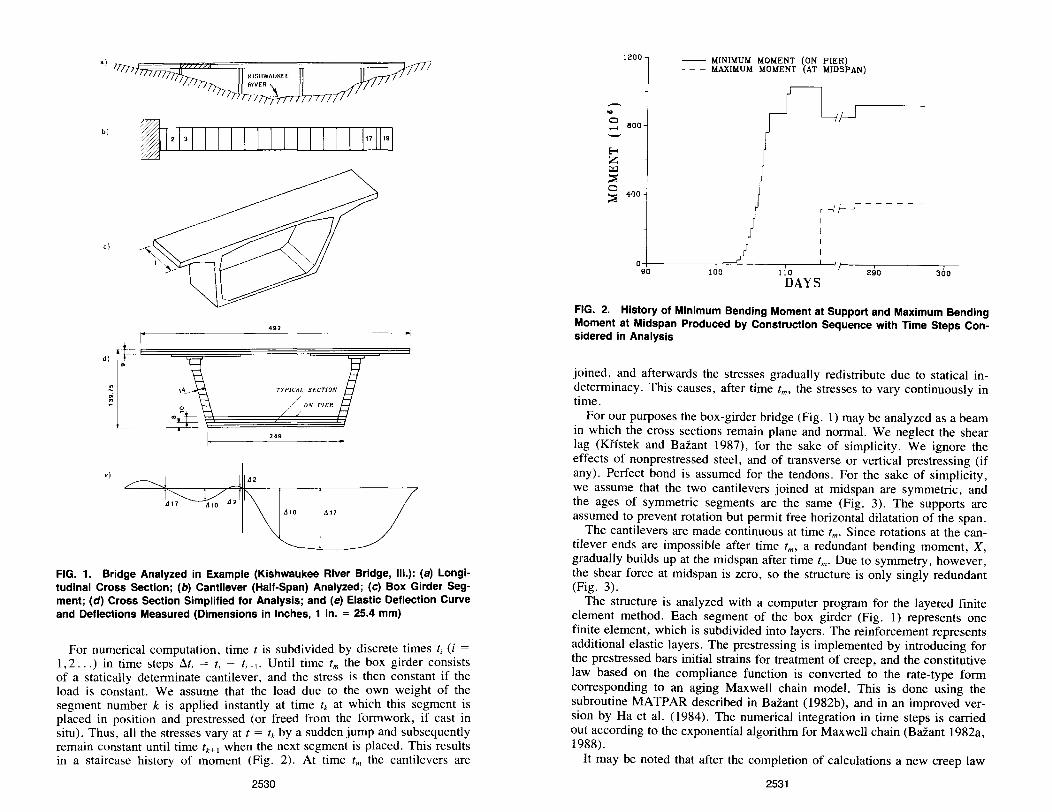
FIG. 3. Change of Structural System and Moment Redistribution

of concrete that is more realistic, simpler to use, and better justified phys­ically was developed (Bazant and Prasannan 1988). Through a certain trans­formation of time, the model can be reduced to a nonaging Kelvin chain, which would allow a simpler solution method than that used here.

Random Parameters for Creep and Shrinkage We adopt the same probabilistic approach as in Bazant and Liu (1985)

and Madsen and Bazant (1983); see also Kfistek and Bazant (1987) for all the approximations and simplifications involved. For the deterministic basis, the BP model from Bazant and Panula (1978, 1980, 1982) is used. The random errors of model are introduced through uncertainty factors 6], 62 , 63

as follows:

Esh(t, to) = 91EshookhS(t, to) ........................................... (1)

J(t,t') = 9{~0 + co(t,n] + 93[Cd(t,t',to) - Cp(t,t',to)] ............... (2)

in which to = the age at the start of drying; t' = the age when the load is applied; coefficients Eshoo, kh, Eo and functions S, Co, Cd and Cp are defined in Bazant and Panula (1978); Eo = the asymptotic modulus; CoCt, t') = the basic creep compliance (i.e., compliance at constant moisture content); Cd(t, t' , to) = an additional compliance due to simultaneous drying; and Cit, t' ,to) = a further correction due to drying which is negligible except for very thin members after a long period of drying (here we use Cp = 0).

In addition to uncertainty factors 6" 62 and 63 , we consider that, in the BP model, the environmental relative humidity h, concrete strength f:, water­cement ratio w/c, gravel-cement ratio g/c, and cement content c are also random. Thus, we have altogether eight random material parameters 6; (i = 1,2, ... ,8): 6" 62 , 63 , 64 = h, 65 , 66 = w/c, 67 = g/c, and 68 = c.

Because the strength is correlated to the water-cement ratio according to the approximate relation f: = [1/(w/c) - 0.5] x 3,300 psi, the random parameter for strength has been introduced as the uncertainty factor 65 of

2532

TABLE 1. Example of Set of 16 Random Samples of Eight Random Parameters for Latin Hypercube Sampling

Run 8, 82 83 8. 85 86 87 8s (1 ) (2) (3) (4) (5) (6) (7) (8) (9)

1 13 11 5 10 13 8 16 6 2 8 I3 4 2 11 4 6 8 3 2 9 6 3 2 12 13 2 4 5 2 I3 16 IO 1 4 1 5 11 5 15 9 7 IO I 5 6 3 4 8 6 4 2 15 7 7 7 8 9 II 12 11 IO 13 8 1 IO 11 12 16 5 7 15 9 IO 14 14 4 15 7 3 4

IO 4 3 16 13 3 13 2 12 II 16 16 IO 8 9 3 9 II 12 6 12 12 7 I 16 14 9 13 15 7 7 14 14 15 8 14 14 14 I 3 I 5 14 12 16 15 12 6 2 15 8 6 5 3 16 9 15 I 5 6 9 II JO

this relation; i.e., f: = 65 [1/(w/c) - 0.5] x 3,300 psi. The expectations and the coefficients of variation of the random parameters are listed in Table 1; their values were justified in Madsen and Bazant (1983). The remaining parameters of the BP model are considered, for the present calculation, as deterministic: initial relative humidity h = 1, temperature T = 23° C, shape factor k, = 1, sand-cement ratio s / c = 1. 75, age at the start of drying of each segment to = 3 days, and effective thickness of the walls of the box girder D = 12 in.

The calculation was applied, as an example, to the Kishwaukee River Bridge in Illinois, for which the concrete mix per cubic yard was: 658 lb of cement, 289 lb of water, 1,864 lb of gravel, 1,150 lb of sand, and 4.5% of air. The slump was 3 ± 1 in. The wall thickness D is variable within the cross section and along the box girder. Although the effect of this variation is quite important for the differences in the creep properties, it must be left for a separate, more-extensive investigation dealing with the effect of mois­ture diffusion through the walls of the girder. In practice, often the values of the initial prestressing forces at anchors as well as the friction losses along the tendon are not controlled very accurately. All the values Fk(tk) should then also be considered as additional random variables 69 , 610 , 61" ••••

It should .also be kept in mind that parameters 6" ... , 68 actually represent a random field over the box girder. Here we assume that the value of each of them is uniform over the entire girder, which is a simplification. Fur­ther:nore, the environmental humidity is in reality a random process in time (Bazant and Wang 1983), as well as a random field along the surface.

BAYESIAN STATISTICAL PREDICTION BY SAMPLING

. In the initial w?rk on Bayesian statistical extrapolation of measured short­tIme creep comphance (Madsen and Bazant 1983), an analytical solution was

2533

rendered possible by a simplification and transformation which made the response a linear function of only two random parameters. Such a simpli­fication is insufficient for predicting the response of a structure; the depen­dence on random parameters in nonlinear and more than just two random material parameters are needed. Bazant (1985) showed that, for nonlinear­izable problems, Bayesian statistical predictions can in general be obtained by a certain modification of the latin hypercube sampling (McKay 1980; McKay et aI. 1976, 1979). BaZant et aI. (1987) applied this method to shrinkage extrapolation. We will apply this method to a bridge.

Let Y; (i = 1,2, ... ,/) at times t; be the long-time effects of creep or shrinkage that we want to predict, and let Xm (m = 1,2, ... ,M) at times t:n

be the short-time effects of creep or shrinkage that have been measured and which we want to use for improving the predictions. Y; may be either the long-time creep or shrinkage strains, or the long-time structural effects, such as the maximum deflection of the box girder, the maximum bending moment or the span shortening at, say 5, 10, 20, and 40 years. Xm may be, for example, the strains of a control cylinder or the box girder deflections at, say, 5 days, 7 days, 28 days, and 5 months.

The values of Y; and Xm that may be predicted on the basis of the available information (i.e., without taking the measurements Xm into account) will be denoted as Y; and X~. The values of Y; may be predicted as certain known functionsy; of the random parameters, i.e., Y; = y;(6), where 6 = (e l ,e2, •. • ,eN )

= vector of random parameters. These functions need not be defined by an explicit formula; they are normally defined by a computer algorithm (pro­gram), which is the case for the present bridge. Predictions can be also ob­tained for the short-time effects, and their predicted values, which generally differ from the measured values X~, may again be regarded as functions of 6; X~ = xm(6). Functions y;(6) and xm(6) are nonlinear. They are defined by the finite element program for box-girder deflections or bending moments.

Statistical analysis of numerous test data from the literature yielded cer­tain, albeit limited, information on the statistical properties of the random parameters eJ, ... , eN (Bazant and Panula 1978, 1980, 1982; Madsen and Bazant 1983; Tsubaki et al. 1986; Bazant and Zebich 1983). This may be regarded as the prior statistical information, characterized by the prior prob­ability density distributions !~(en) with means ij~ and standard deviations s~ (n = 1,2, ... ,N). With this knowledge it is possible to predict the statistical distributions!!' of X~ = xm(6) and compare them to the available short-time measurements Xm of known distributions I!, The objective is to use this comparison to improve, or update, the statistical information on the random parameters en" This improved statistical information may be characterized by updated, or posterior, distributions !~(en)' from which the updated, or pos­terior, distributions frey;') of the long-time effects Y; may be obtained ac­cording to functions y;(6), The double primes are used to distinguish the posterior characteristics from the prior characteristics, which are labeled by single primes,

As shown in general by Bazant (1985) and applied to shrinkage by Bazant et al. (1987), the method of latin hypercube sampling can be effectively extended to problems of the present type. In this sampling method, the known distribution !;'(en ) of each input parameter en is partitioned into K intervals ae(k) (strata) of equal probability 11K (k = 1, ... ,K). The subdivision may be obtained according to the cumulative probability distribution, as illus-

2534

1

-----;(' -if-16- t'A,- --Jf I

,II I

:I I I I I

:I I I

I I I

f I I

f I I

f I I

I I

f I I

I I I

I I I

-------,;1 I I

I I ...;(1 I I

----I I I I

1J i

FI~: 4. SubdiVision of Random Parameter Range Into Intervals of Equal Prob­ability and Determination of Sampling Values

trated ,in Fig. 4. The number of random parameter samples in latin hypercube sampling must be chosen to be the same as the number of computer runs to be made, and from each interval the random parameter value must be sam­pled exactly once; i.e., it must be used in one and only one computer run. The sampled value ne.ed not be taken randomly from the interval, but may be taken at the centroid of the interval (Fig. 4).

The random selection O! the intervals ae(k) to be sampled for a particular computer run ~an be carned out as follows. With each random parameter one ma,y associate a sequence of integers representing a random permutation of th~ Illteger~ 1, 2, ... , K. For 16 intervals (K = 16), such random per­mutat~ons .are Illustrated in the columns of Table I. A different random per­mutatlO~ IS used for each column (each en). Thus, each interval number appears III each column of Table 1 once and only once. The individual latin hypercube samples. are then represented by the rows in Table I. According to the creep or shnnkage prediction model, one can then calculate for each such sample ~~k) (n = I, ... , N) the effects X~k) that correspond to the mea­s~~k~d short-time e!fects Xm , and _also the corresponding long-time effects Y! ' The ,m~an p!,or prediction. X~ for the measured effects X

m, the mean

pn~r ~redlctlOn y; of the long-time effects, and the corresponding standard deViatIOns then are

1 K X' = - 2: X,(k)

m K k=l m,

, [1 K ] 1/2 s! = - 2: (X~k) - X~)2 K k~1

(m = 1,2, . .. ,M) ............................................... (3a) , [1 K ] 1/2 S~ = - 2: (y~k) _ y~)2

K k~1

1 K Y' = - 2: y,(k)

m K k~1 m,

(m = 1,2, ... ,M) ... , ...... , . , . , .... , .. , . , . ..................... (3b)

2535

1.1 .... ----------------,

..-.,0.9

2:i ---ZO.7 o E=: u ::3 0.5

r... tJ;:l ~

0.3

00000 PRIOR DISTRIBUTION -- PDSTERIDR DISTRIBUTION

16 SAIotPLES

1.1 -,----------------,

..-.,0.9

2:i ZO.7 o E=: u r:g 0.5

r... tJ;:l ~

0.3

00000 PRIOR DISTRIBUTION -- POSTERIOR DISTRIBUTION

16 SAIotPLES

0.1 +-~-f-~..,-~--r-~..,-~__r-.------l -3 -2 -1 3 -3

00000 PRIOR DISTRIBUTION -- POSTERIOR DISTRIBUTION

16 SAIotPLES

-2 -1

PROBABILITY SCALE

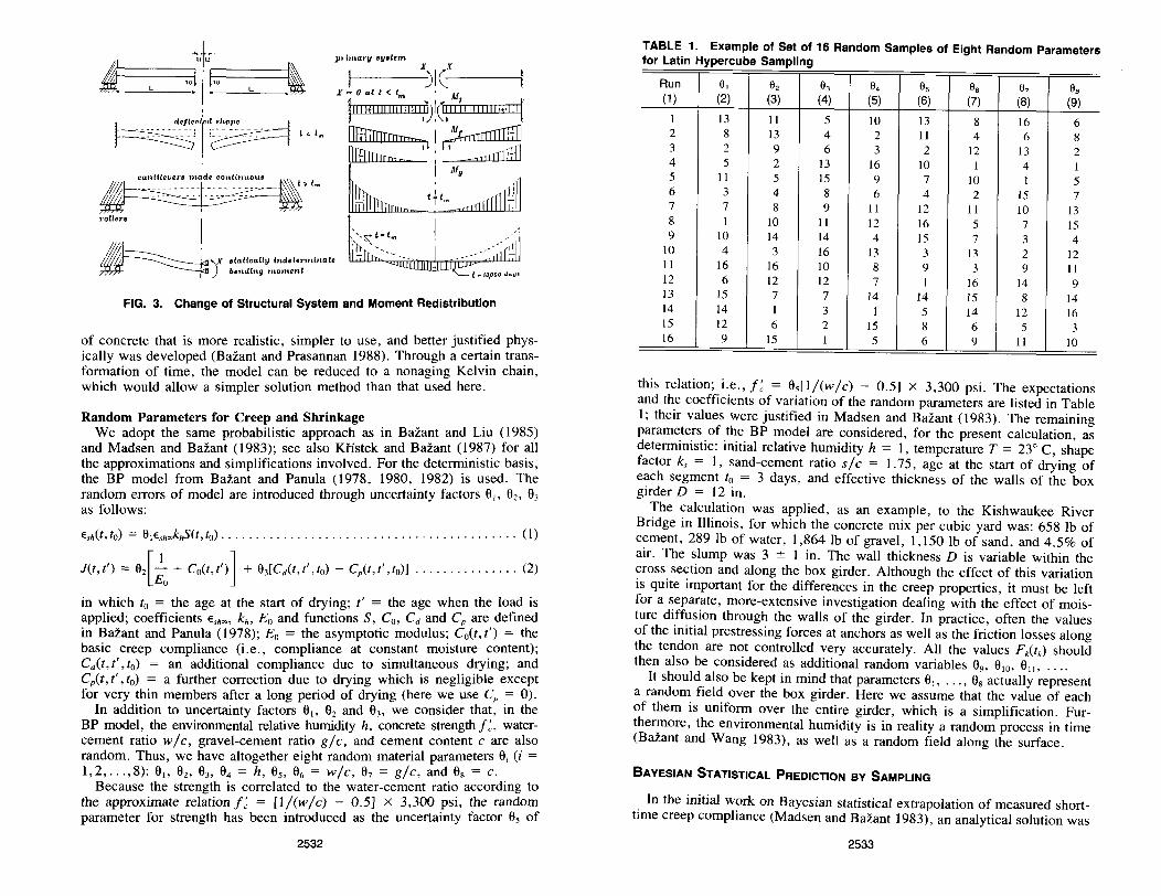
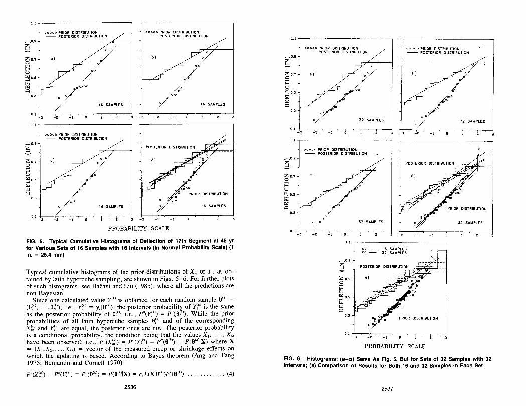
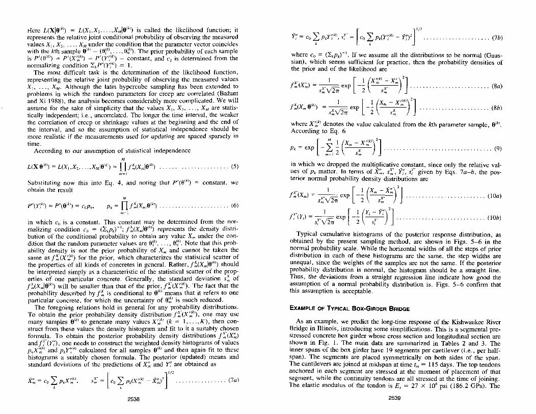
FIG. 5. Typical Cumulative Histograms of Deflection of 17th Segment at 45 yr for Various Sets of 16 Samples with 16 Intervals (In Normal Probability Scale) (1 in. = 25.4 mm)

Typical cumulative histograms of the prior distributions of Xm or Yi , as ob­tained by latin hypercube sampling, are shown in Figs. 5-6. For further plots of such histograms, see Bazant and Liu (1985), where all the predictions are non-Bayesian.

Since one calculated value y~k) is obtained for each random sample O(k) = (fW), ... , at»; i.e., y~k) = Yi(O(k», the posterior probability of y~k) is the same as the posterior probability of a~k); i.e., p"(y~k» = p"(a~k». While the prior probabilities of all latin hypercube samples a~k) and of the corresponding X~) and y)k) are equal, the posterior ones are not. The posterior probability is a conditional probability, the condition being that the values XI, ... , XM

have been observed; i.e., P"(X~» = p"(y~k» = P"(O(k» = p(o(k)IX) where X = (XloXz, ... ,XM ) = vector of the measured creep or shrinkage effects on which the updating is based. According to Bayes theorem (Ang and Tang 1975; Benjamin and Cornell 1970)

P"(X~» = p"(y~k» = p"(O(k» = p(o(k)IX) = cIL(Xlo(k»p'(O(k» ............ (4)

2536

1.1 .... ----------____ --,

ZO.7 o E=: u ::3 0.5

r... tJ;:l ~

0.3

00000 PRIOR DISTRIBUTION -- POSTERIOR DISTRIBUTION

32 SAIotPLES

0.1_ -+3::-~'-2::-~'--1 ~---'-~....,-r----,-~--J

1.1 -,---------------....,

_0.9

2:i Z 0.7 o E=: U ~0.5

"'" tJ;:l ~

0.3

0.1 ":3

00000 PRIOR DISTRIBUTION -- POSTERIOR DISTRIBUTION

cj

32 SAIotPLES

-2 -1

1.1

-3

00 16 SAIotPLES 00 32 SAIotPLES

_0.9

2:i POSTERIOR

ZO.7 ej 0

E=: u ::3 0.5

r... tJ;:l ~

0.3

00000 PRIOR DISTRIBUTION -- POSTERIOR DISTRIBUTION

b)

00

32 SAIotPLES

-2 -1 o

-2 -1

PRIOR DISTRIBUTION

0.1 -3 -2 -1

PROBABILITY SCALE

FIG. 6. Histograms: (a-d) Same As Fig. 5, But for Sets of 32 Samples with 32 Intervals; (e) Comparison of Results for Both 16 and 32 Samples in Each Set

2537

dere L(xla(k» = L(Xj,X2"" ,xMla(k» is called the likelihood function; it represents the relative joint conditional probability of observing the measured values X" X 2 , ••• , XM under the condition that the parameter vector coincides with the kth sample O(k) = (e~k), ... , e;;». The prior probability of each sample is p'(e(k» = p'(X~k» = p'(y;(k» = constant, and c, is determined from the normalizing condition ~kPII(y~k» = 1.

The most difficult task is the determination of the likelihood function, representing the relative joint probability of observing the measured values X" ... , XM • Although the latin hypercube sampling has been extended to problems in which the random parameters for creep are correlated (Bazant and Xi 1988), the analysis becomes considerably more complicated. We will assume for the sake of simplicity that the values X" X 2 , ••• , XM are statis­tically independent; i.e., uncorrelated. The longer the time interval, the weaker the correlation of creep or shrinkage values at the beginning and the end of the interval, and so the assumption of statistical independence should be more realistic if the measurements used for updating are spaced sparsely in time.

According to our assumption of statistical independence M

L(Xlo(k» = L(X, ,X2 , ••• ,xMlo(k') = Il 1;'(Xmlo(k» ...................... (5) m=1

Substituting now this into Eq. 4, and noting that p'(e(k» = constant, we obtain the result

M

Pk = Il 1;'(Xmlo(k) ...................... (6) m=l

in which Co is a constant. This constant may be determined from the nor­malizing condition Co = (~kPk)-'; /;'(XmIO(k» represents the density distri­bution of the conditional probability to obtain any value Xm under the con­dition that the random parameter values are e\k), ... , e;;). Note that this prob­ability density is not the prior probability of Xm and cannot be taken the same as 1~'(X~k» for the prior, which characterizes the statistical scatter of the properties of all kinds of concretes in general. Rather, /;'(XmIO(k» should be interpreted simply as a characteristic of the statistical scatter of the prop­erties of one particular concrete. Generally, the standard deviation s! of /!(XmIO(k» will be smaller than that of the prior, /;"(X~k». The fact that the probability described by I;' is conditional to O(k) means that it refers to one particular concrete, for which the uncertainty of e~) is much reduced.

The foregoing relations hold in general for any probability distributions. To obtain the prior probability density distribution /!'(X~k», one may use many samples O(k) to generate many values X~k) (k = 1, .. . ,K), then con­struct from these values the density histogram and fit to it a suitably chosen formula. To obtain the posterior probability density distributions /!"(X~) and/r(y;'), one needs to construct the weighted density histograms of values PkX'~k) and Pky,;(k) calculated for all samples O(k) and then again fit to these histograms a suitably chosen formula. The posterior (updated) means and standard deviations of the predictions of X~ and Y7 are obtained as

s~' = [co ~ Pk(X~k) - X~)2 J '/2 ................ (7a) X" = c '" P X,(k) m OL.Jkm, k

2538

(7b)

where Co = (~kPk)-" If we assume all the distributions to be normal (Gaus­sian), which seems sufficient for practice, then the probability densities of the prior and of the likelihood are

1 [1 (X'(k) - X,)2] I;"(X;") = x',;;:c exp -- m x' m •• , , , • , , •.•.••••••••••••• (8a)

Sm v 21T 2 Sm

I;'(xmlo(k» = x, 1;;;- exp [_~ (Xm _xX~k»)2] ...................... (8b) SmV21T 2 Sm

where X~k) denotes the value calculated from the kth parameter sample, O(k). According to Eq. 6

Pk = exp [-f ~ (Xm _xX~k»)2] '" .......... '" .................. (9) m~' 2 Sm

in which we dropped the multiplicative constant, since only the relative val­ues of Pk matter. In terms of X~, s~', y;" sr given by Eqs. 7a-b, the pos­terior normal probability density distributions are

1 [

1 (X _,,)2J X" m - Xm 1m (Xm ) = X",;;;- exp -- X" •.••••••.•.•.•••.•.•••••• (lOa)

SmV21T 2 Sm

1 [ 1 (Y -,,)2J

y" i - Y i I, (YJ = Y",;;;- exp -- -y-.. - ..... " ..... , ............... (lOb) Si v 21T 2 Si

Typical cumulative histograms of the posterior response distribution, as obtained by the present sampling method, are shown in Figs. 5-6 in the normal probability scale. While the horizontal widths of all the steps of prior distribution in each of these histograms are the same, the step widths are unequal, since the weights of the samples are not the same. If the posterior probability distribution is normal, the histogram should be a straight line. Thus, the deviations from a straight regression line indicate how good the assumption of a normal probability distribution is. Figs. 5-6 confirm that this assumption is acceptable.

EXAMPLE OF TYPICAL BOX-GIRDER BRIDGE

As an example, we predict the long-time response of the Kishwaukee River Bridge in Illinois, introducing some simplifications. This is a segmental pre­stressed concrete box girder whose cross section and longitudinal section are shown in Fig. 1. The main data are summarized in Tables 2 and 3. The inner spans of the box girder have 19 segments per cantilever (i.e., per half­span). The segments are placed symmetrically on both sides of the span. The cantilevers are joined at midspan at time tm = 115 days. The top tendons anchored in each segment are stressed at the moment of placement of that segment, while the continuity tendons are all stressed at the time of joining. The elastic modulus of the tendon is Es = 27 X 106 psi (186.2 GPa). The

2539

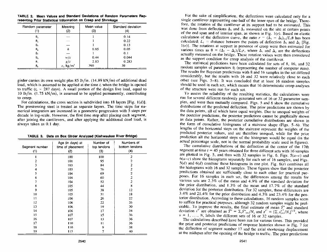
TABLE 2. Mean Values and Standard Deviations of Random Parameters Rep­resenting Prior Statistical Information on Creep and Shrinkage

Random parameter Meaning Mean value Standard deviation (1 ) (2) (3) (4)

6, - 1 0.14 62 - 1 0.22 63 - 1 0.13 64 h 0.65 0.05 6, - 1 0.1 66 w/c 0.44 0.044 67 g/c 2.83 0.283 68 c, kg/m3 390 39

girder carries its own weight plus 85 Ib/in. (14.89 kN/m) of additional dead load, which is assumed to be applied at the time t, when the bridge is opened to traffic (t, = 287 days). A small portion of the design live load, equal to 10 Ib/in. (1.75 kN/m), is assumed to be applied permanently, contributing to creep.

For calculations, the cross section is subdivided into 18 layers [Fig. l(d)). The prestressing steel is treated as separate layers. The time steps for nu­merical integration are increased in a geometric progression with 5 steps per decade in log-scale. However, the first time step after placing each segment, after joining the cantilevers, and after applying the additional dead load, is always taken as 0.1 day.

TABLE 3. Data on Box Girder Analyzed (Kishwaukee River Bridge)

Age (in days) at Number of Numbers of Segment number time of placement top tendons bottom tendons

(1 ) (2) (3) (4)

1 100 100 2 2 101 95 2 3 103 84 2 4 103 76 2 5 104 69 2 6 104 60 2 7 104 52 2 8 105 44 8 9 105 38 12

10 105 31 18 11 106 26 22 12 106 22 26 13 106 19 30 14 106 17 34 15 107 15 36 16 107 13 36 17 110 11 36 18 110 9 38 19 115 7 40

2540

For the sake of simplification, the deflections were calculated only for a single cantilever representing one-half of the inner span of the bridge. There­fore, the rotation of the cantilever at its support had to be estimated. This was done from deflections ill and il2 measured on the site at certain points of the end span and of interior span, as shown in Fig. l(e). Based on elastic calculation of the deflection curve, the ratio r = (ill - il2)el/Llfj has been calculated; Ll = distance between the points of deflection ill and il2 [Fig. 1 (e)). The rotations at support in presence of creep were then estimated for various times as fj = (il2 - ill)/Llr, where ill and il2 are the deflections actually measured on the bridge. These rotation values were then considered as the support condition for creep analysis of the cantilever.

The statistical predictions have been calculated for sets of 8, 16, and 32 random samples of parameters fjt (representing the number of computer runs). The results for Bayesian predictions with 8 and 16 samples in the set differed considerably, but the results with 16 and 32 were relatively close to each other (see Figs. 5-8). It was concluded that at least 16 random samples should be used in each set, which means that 16 deterministic creep analyses of the structure were run for each set.

To assess the reliability of the resulting statistics, the calculations were run for several different randomly generated sets of 16 or 32 parameter sam­ples, and were then mutually compared. Figs. 5 and 6 show the cumulative distributions of the predicted deflection. The prior predictions are shown by the data points, all of which have equal weights. Due to unequal weights of the posterior predictions, the posterior predictions cannot be graphically shown as data points. Rather, the posterior cumulative distributions are shown in the form of cumulative histograms of a staircase shape (Figs. 5-6). The lengths of the horizontal steps on the staircase represent the weights of the predicted posterior values, and are therefore unequal, while for the prior prediction all the horizontal steps of the histogram would be equal (in the actual percentage scale, not in the normal probability scale used in figures).

The cumulative distributions of the deflection at the center of the 17th segment at time t = 45 years obtained for three different sets with 16 samples are plotted in Fig. 5, and then with 32 samples in Fig. 6. Figs. 5(a-c) and 6(a-c) show the histograms separately for each set of 16 samples, and Figs. 5(d) and 6(d) combine these histograms in one plot. Fig. 6(e) combines all the histograms with 16 and 32 samples. These figures show that the posterior predictions obtained are sufficiently close to each other for practical pur­poses. For 16 samples in each set, the differences among the results for various sets are 2.3% of the mean and 4.9% of the standard deviation for the prior distribution, and 1. 3% of the mean and 17.7% of the standard deviation for the posterior distribution. For 32 samples, these differences are 3.4% and 21.4% for the prior distribution and 4.3% and 23.4% for the pos­terior distribution. According to these calculations, 16 random samples seem to suffice for practical purposes, although 32 random samples might be pref­erable. To improve the results, the final estimate of mean Y" and standard deviation sY" are obtained as Y" = 2.vY"(v)/Ns and sY" = [2.vsr::/Ns

) 1/2, where v = I, ... , Ns labels the different sets of 16 or 32 samples.

The calculations described have been run for various times. This provided the prior and posterior predictions of response histories shown in Fig. 7 for the deflection of segment number 17 and the axial shortening displacement at the midspan after the opening of the bridge to traffic. The prior predictions

2541

1.2.,-----------------,

••••• USED FOR BAYESIAN PREDICTION 1.0 cccoc IGNORED FOR BAYESIAN PREDICTION

---Z ~ O.B

Z 0 0.6

E=: U

0.4

"'" ..... r..

"'" 0.2 0

0.0

-0.2 0.1

1.2

---Z ~ 0.8

Z 0 0.6

E=: U

"'" 0.4

-l ~

"'" 0.2 0

0.0

-0.2 0.1

1.2

---

-- POSTERIOR OISTRIBUTION . - - PRIOR DISTRIBUTION

a) 0

6'

/ //' !-~

/

16

10 100 1000

-- POSTERIOR DISTRIBUTION - - PRIOR DISTRIBUTION

c) 0

6' /

/ /

/

SAIAPLES

10000 100000

/

°V '" /' ...- ..... --/ /

/ / -.- .......

16 SAIotPLES

10 100 1000 10000 100000

Z -- POSTERIOR DISTRIBUTION ~ 0.8 - - PRIOR DISTRIBUTION

Z e) 0 0.8

o 6'

E=: U

0.4

"'" ,

..... r..

"'" 0.2 0

0.0 32 SAIotPLES

-0.2

••••• USED FOR BAYESIAN PREDICTION cocco IGNORED FOR BAYESIAN PREDICTION

-- POSTERIOR DISTRIBUTION - - PRIOR DISTRIBUTION

b)

o /

/ /' /

/

16 SAIAPLES

0.1 10 100 1000 10000 100000

••••• USED FOR BAYESIAN PREDICTION cocco IGNORED rOR BAYESIAN PREDICTION

-- POSTERIOR DISTRIBUTION - - PRIOR DISTRIBUTION

d) 0

6' /

"

/

/~ ~/

/

32 SAIotPLES

0.1 10 100 1000 10000 100000

••••• USEe FOR BAYESIAN PREDICTION ocooc IGNORED FOR BAYESIAN PREDICTION

-- POSTERIOR DISTRIBUTION - - PRIOR DISTRIBUTION

o 6'

32 SAIotPLES

0.1 10 100 1000 10000 100000 0.1 10 100 1000 10000 100000

DAYS

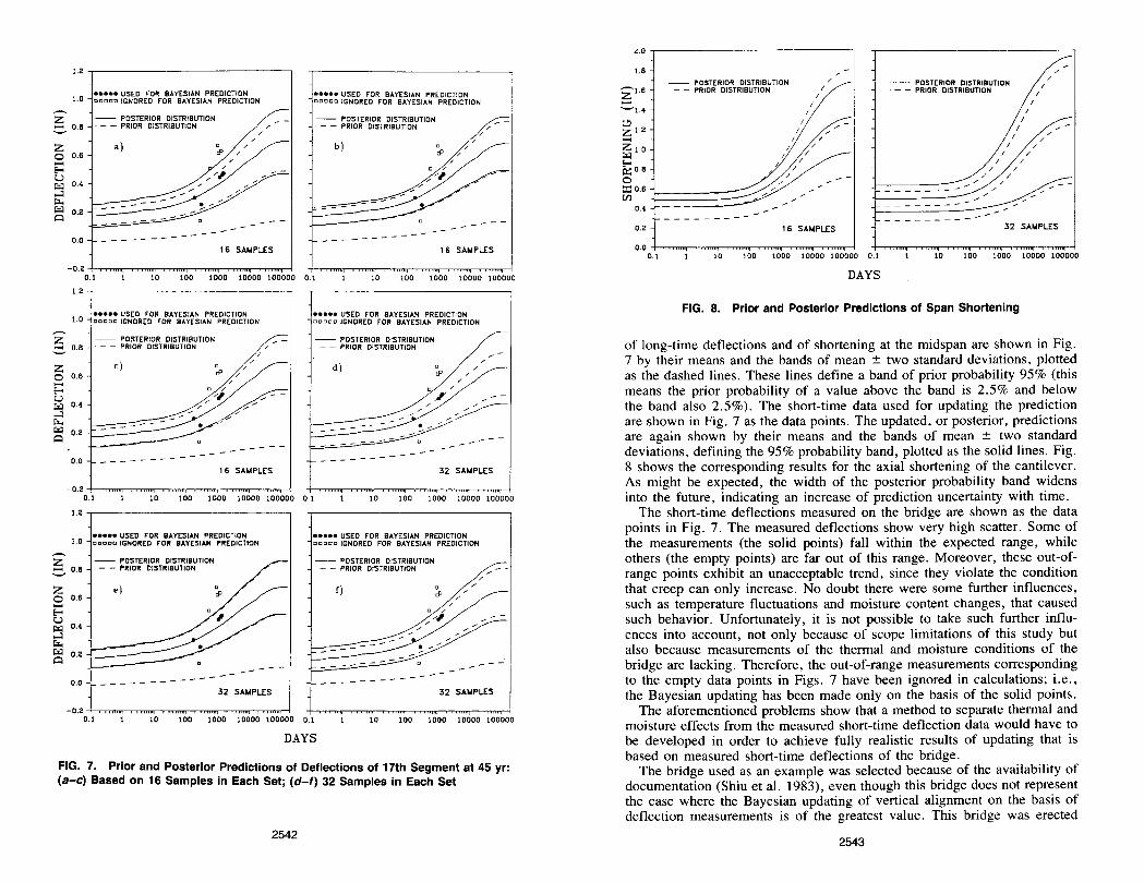
FIG. 7. Prior and Posterior Predictions of Deflections of 17th Segment at 45 yr: (a-c) Based on 16 Samples in Each Set; (d-f) 32 Samples in Each Set

2542

<.0.----------------,

1.8

c.!:I Zl.2

~1.0 ~08 o

-- POSTERIOR DISTRIBUTION - - PRIOR DISTRIBUTION

/, / h /

/

I

/

I

/

/

/ /

/

gJ 0.6 r::==:::==::::: 0.4 J

0.2 16 SAIotPLES

0.0 +-~mnr~~,.....,.~"",~,",,,,~~nr-~~ 0.1 10 100 1000 10000 100000 0.1

DAYS

-- POSTERIOR DISTRIBUTION - - PRIOR DISTRIBUTION

/ /

/

I

/ /

I

/

/

/

/

/ /

32 SAIotPLES

10 100 1000 10000 100000

FIG. 8. Prior and Posterior Predictions of Span Shortening

of long-time deflections and of shortening at the midspan are shown in Fig. 7 by their means and the bands of mean ± two standard deviations, plotted as the dashed lines. These lines define a band of prior probability 95% (this means the prior probability of a value above the band is 2.5% and below the band also 2.5%). The short-time data used for updating the prediction are shown in Fig. 7 as the data points. The updated, or posterior, predictions are again shown by their means and the bands of mean ± two standard deviations, defining the 95% probability band, plotted as the solid lines. Fig. 8 shows the corresponding results for the axial shortening of the cantilever. As might be expected, the width of the posterior probability band widens into the future, indicating an increase of prediction uncertainty with time.

The short-time deflections measured on the bridge are shown as the data points in Fig. 7. The measured deflections show very high scatter. Some of the measurements (the solid points) fall within the expected range, while others (the empty points) are far out of this range. Moreover, these out-of­range points exhibit an unacceptable trend, since they violate the condition that creep can only increase. No doubt there were some further influences, such as temperature fluctuations and moisture content changes, that caused such behavior. Unfortunately, it is not possible to take such further influ­ences into account, not only because of scope limitations of this study but also because measurements of the thermal and moisture conditions of the bridge are lacking. Therefore, the out-of-range measurements corresponding to the empty data points in Figs. 7 have been ignored in calculations; i.e., the Bayesian updating has been made only on the basis of the solid points.

The aforementioned problems show that a method to separate thermal and moisture effects from the measured short-time deflection data would have to be developed in order to achieve fully realistic results of updating that is based on measured short-time deflections of the bridge.

The bridge used as an example was selected because of the availability of documentation (Shiu et al. 1983), even though this bridge does not represent the case where the Bayesian updating of vertical alignment on the basis of deflection measurements is of the greatest value. This bridge was erected

2543

very fast, each half-span within about 15 days. Consequently, the measure­ments during erection give relatively little information on creep, and have a lesser importance for long-time deflection than measurements on a bridge erected slower, as is the case for some other methods of construction.

Segmental box-girder bridges should be designed not for the mean re­sponse, as is the practice now, but for extreme response, such as the 95% confidence limits (represented by the mean ± two standard deviations). The present method makes it possible not only to make statistical predictions on the basis of the prior statistical information for all concretes from the lit­erature, but also to update the predictions on the basis of deflection mea­surements made during construction. Based on such prediction, one should adjust during construction the vertical alignment of the remaining segments. However, to apply this method in practice, the effects of daily and seasonal fluctuations of environmental humidity and temperature must be eliminated from the short-time data used for updating, as already emphasized. This problem deserves further study.

As an alternative use of the present statistical approach, the prior predic­tions can also be updated on the basis of short-time laboratory measurements of concrete specimens of the particular concrete to be used in the structure. In that case, of course, the problem of separating the effect of random en­vironmental fluctuations does not arise. This type of updating is certainly not as relevant as the measurements taken on the bridge during construction, but still is no doubt better than no updating at all, and its practical application is feasible right now.

It should also be recognized that our stress-strain relation in Eq. I is a simplified one. More realistically, the local values of pore humidity and temperature, which need to be solved from the diffusion equation, affect the creep rate. Nonuniformity of shrinkage and creep leads to residual stresses and cracking or tensile strain-softening. At present, it is not yet clear how important these effects are for the statistical predictions.

Finally, it should be kept in mind that the Bayesian approach itself is not perfect from the probabilistic viewpoint. The results depend only on the dis­tributions of the prior and of the data but not on the number of prior data and the number of measurements used for the updating. Obviously, if the prior data consist of 10,000 points and the update consists of only 6 points, the prediction should be closer to the prior than if the update consists of 1,000 points, the prior data being same. But the Bayesian approach cannot distinguish between these two cases. In this respect, there is room for further fundamental improvement of the probability method.

ALTERNATIVE METHOD FOR SHARP OR REMOTE LIKELIHOOD

Our calculation procedure breaks down if the likelihood distribution is much sharper than the prior distribution or is too remote from the prior. In these situations, the response values for various parameter samples very sel­dom fall within the range of the observed data (the update), and an extremely large number of samples would be required to obtain a sufficient number (at least 8) of response values within the range of the data. In such a case, all coefficients Pk are almost zero, and the results are meaningless.

An alternative procedure, also proposed by Bazant (1985), can cope with such situations, provided that the tails of the distributions can be assumed

2544

to be gaussian (normal). Paying, at first, no attention to the prior informa­tion, we need to extrapolate the given data Xm to obtain predictions Yi for long times. This can be accomplished, e.g., by the Levenberg-Marquardt nonlinear optimization algorithm, for which a standard subroutine is avail­able. Disregarding the prior information, this subroutine is used to calculate the optimum random parameter values en = ii~, which minimize the sum of squares of the deviations of the response predictions ~ from the observed data Xm at times tm • This subroutine not only estimates the optimum values of random parameters en, but it also estimates (on the basis of tangential linearizations) their standard deviations s~. Then, assuming en to have normal distributions with means ii~ and standard deviations s~, one can generate latin hypercube samples erik) of the random parameters en on the basis of the up­dating data alone (i.e., without any regard to the prior). For each of these samples one can calculate the long-time responses Y7(k) (i = 1,2, ... ,/). Then, considering ~ll the generated values Y7(k) for each time t;, one can calculate their mean Y;' and standard deviation si".

The extrapolated statistical information yr and s;' may be regarded as a set of update data for the long time t; and confronted in the Bayesian sense with the predictions Y; from the prior. For this purpose one needs to generate the prior latin hypercube samples e'~k) of random parameters en, and calculate the corresponding responses Y'jk) for all the samples. From these, one can then obtain the mean Y; and the standard deviation st of the prior prediction, for each time t;, as described before.

Assuming normal distributions for both the extrapolated measured data and the predictions from the prior, we now have an elementary Bayesian problem, consisting of a combination of a normal prior with a normal like­lihood (representing the extrapolated measurements). As is well known (Box and Tiao 1973:74), the posterior distribution is then also normal and its mean and standard deviation are given by

(SY")-2yo + (SY')-2 y' y~' = I I f I

, (STY2 + (si')-2 ' (si')-2 = (S;")-2 + (si')-2, ..... , ......... (11)

The measured short-time data Xm are usually quite limited and do not suf­fice to obtain full statistical information on all the para!11eters en" Thus, if one attempts to determine from Xm the optimum values e~ of all the param­eters en, the problem is ill-conditioned, because very different values of en yield nearly equally good fits of Xm , although the corresponding predictions Y, might be very different. In such a case, the number of random parameters en for which the optimum values ii~ are sought must be reduced, and for the remaining en one must use the mean values of the prior. For rather limited update data Xm , one would optimize from Xm only two parameters, e1 and e2 (and assume e3 = e2). For more extensive update data Xm , one can op­timize e1, e2 , and e3 •

Keep in mind, too, that if the distribution of the data is extremely sharp, or if it is too remote from the prior, then Bayesian updating is of dubious value. A simple extrapolation of the given short-time data without any regard to the prior makes more sense.

CONCLUSIONS

1. Predictions of confidence limits for long-time deflections and internal forces can be improved by Bayesian analysis based on short-time measurements.

2545

2. The Bayesian analysis can in general be carried out by latin hypercube sampling of random parameters in the creep prediction model. No linearization with regard to the random parameters is necessary, and all the known random parameters of the creep prediction model, such as the BP model, can be con­sidered.

3. The sampling approach reduces the probabilistic problem to a series of deterministic structural creep analyses for various samples of random material parameters. Differences in age between the bridge segments, as well as a change in the structural system from statically determinate to indeterminate, can be taken into account.

4. An example of Bayesian statistical predictions for one particular recently constructed bridge demonstrates feasibility of the proposed new method.

ACKNOWLEDGMENT

Partial financial support under U.S. National Science Foundation Grants No. FED-7400 and MSM-88l5l66 to Northwestern University is gratefully acknowledged. Thanks are due to K. N. Shiu of Construction Technology Laboratories, Skokie, Ill., for providing information on the construction data and measurements on the Kishwaukee River Bridge.

ApPENDIX. REFERENCES

ACI Committee 109/11. (1982). "Prediction of creep, shrinkage, and temperature effects in concrete structures." ACI SP-2 7, Designing for Effects of Creep, Shrink­age, and Temperature, ACI, Detroit, Mich., 51-93.

Ang, A. H.-S., and Tang, W. H. (1975). Probability concepts in engineering plan­ning and design, vol. 1: Basic principles. John Wiley and Sons, New York, N.Y., 329-359.

Bazant, Z. P. (I 982a). "Mathematical models for creep and shrinkage of concrete." Creep and Shrinkage of Concrete Structures, Z. P. Bazant and F. H. Wittman, eds., John Wiley and Sons, London, U.K., 163-256.

Bazant, Z. P. (1982b). "Input of creep and shrinkage characteristics for a structural analysis program." Materials and Structures (Materiaux et Constructions). RI­LEM, 15(88), Paris, France, 283-290.

Bazant, Z. P. (1983). "Probabilistic problems in prediction of creep and shrinkage effects in structures." Proc., 4th Int. Conf. on Appl. of Statistics and Probability in Soil and Struct. Engrg. Florence, Italy, 325-356.

Bazant, Z. P. (1985). "Probabilistic analysis of creep effects in concrete structures." Proc., IcaSSAR 85, 4th Int. Conf. on Struct. Safety and Reliability. I. Konishi, A. H.-S. Ang, and M. Shinozuka, eds., Kobe, Japan, 1, 331-344.

Bazant, Z. P., et al. (1988). "Material models for structural creep analysis." Math­ematical modeling of creep and shrinkage of concrete. Proc., RILEM Int. Symp. Northwestern Univ., Z. P. Bazant, ed., John Wiley and Sons, Chichester and New York, 99-216.

Bazant, Z. P., and Chern, J. C. (1984). "Bayesian statistical prediction of concrete creep and shrinkage." ACI J., 81(6),319-330.

Bazant, Z. P., and Liu, K. L. (1985). "Random creep and shrinkage in structures: Sampling." J. Struct. Engrg., ASCE, 111(5), 1113-1134.

Bazant, Z. P., and Panula, L. (1978a). "Practical prediction of time-dependent de­formations of concrete," Materials and Struct. Parts I and II: 11(65), 307-328, Parts III and IV: 11(66),415-434, Parts V and VI (1979): 12(69), 169-183.

Bazant, Z. P., and Panula, L. (1980). "Creep and shrinkage characterization for analyzing prestressed concrete structures." Prestressed Concrete Institute J., 25(3), 86-122.

2546

BaZant, Z. P., and Panula, L. (1982). "New model for practical prediction of creep and shrinkage." ACI Special Pub., SP-76, Detroit, Mich., 7-23.

Bazant, Z. P., and Prasannan, S. (1988). "Solidification theory for aging creep." Cement and Concr. Res., 18(6), 923-932.

Bazant, Z: P., and .xi, Y. (1988). "Sampling analysis of concrete structures for creep and shrmkage wIth correlated random material parameters." Probabilistic Engrg. Mech., (in press).

Bazant, Z. P., and Wang, T. S. (1983). "Spectral analysis of random shrinkage stresses in concrete." J. Engrg. Mech., ASCE, 110(2), l73-186.

Bazant, Z. P., Kim, J.-K., Wittmann, F. H., and Alou, F. (1987). "Statistical ex­trapolation of shrinkage data-Part II: Bayesian updating." ACI Materials J., 84(2) ~~1. '

Baz.ant, Z. P., and Zebich, S. (1983). "Statistical linear regression analysis of pre­dIctIOn models for concrete creep and shrinkage." Cement and Concrete Research, 13(6), 869-876.

Benjamin, J. R., and Cornell, A. C. (1970). Probability, statistics and decision for civil engineers. Mc-Graw-Hill Book Co., New York, N.Y., 524-641.

Box, G. E. P., and Tiao, G. C. (1973). Bayesian inference in statistical analysis. Addison-Wesley Publishing Co., Reading, U.K.

CEB-FIP. (1978). Model code for concrete structures. Commite Eurointernational du Beton-Federation Internationale de la Precontrainte, CEB Bulletin No. 124/ 125-E, Paris, France.

Ha,. ~., Osrr~an, M. A., and Huterer, J. (1984). "User's guide: Program for pre­dlctmg shnnkage and creep in concrete structures." Report, File: NK38-26191P, Ontario Hydro, Toronto, Canada.

Kifstek, V., and Bazant, Z. P. (1987). "Shear lag effect and uncertainty in concrete box girder creep." J. Struct. Engrg., ASCE, 113(3), 557-574.

Madsen, H. 0., and Bazant, Z. P. (1983). "Uncertainty analysis of creep and shrink­age effects in concrete structures." ACI J., 80(2), 116-127.

McKay, M. D. (1980). "A method of analysis for computer codes." Report, Los Alamos Nat. Lab., Los Alamos, N.M.

McKay, M. D., Beckman, R. 1., and Conover, W. J. (1979). "A comparison of three methods for selecting values of input variables in the analysis of output from a computer code." Technometrics, 21(2), 239-245.

McKay, M. D., Conover, W. J., and Whiteman, D. C. (1976). "Report on the application of statistical techniques to the analysis of computer code." Los Alamos Sci. Lab. Report LA-NUREG-6526-MS, NRC-4, Los Alamos, N.M.

Shiu, K. N., Daniel, J. P., and Russell, H. G. (1983). "Time-dependent behavior of segmental cantilever concrete bridges." Report, Constr. Tech. Labs., Portland Cement Assoc., Skokie, Ill.

Tsubaki, T., et al. (1988). "Probabilistic models." Mathematical modeling of creep and shrinkage of concrete. Proc., RILEM Intern. Symp. Northwestern Univ., Z. P. Bazant, ed., John Wiley and Sons, Chichester, and New York, 311-384.

2547