Seed and pollen dispersal

Remember from the first lecture that seeds may be dispersed on wind, by water, and by animals. Animal-borne seeds may be carried externally or may be transported until defecated from the gut.

The basic spatial pattern for dispersal is very similar for all mechanisms of dispersal. All show a peak in abundance of dispersed propagules at a short distance from the source plant, then a decline with increasing distance. The rate of decline differs, but all distributions are skewed, with a more-or-less extended tail.

Think of a wind-dispersed seed as one example. Seeds are broken free of the parent (abscised) by a sufficiently strong velocity (a gust possibly) of wind.

The force required to break the seed free explains why the peak of the distribution occurs at some small distance from the parent.

The remainder of the distribution is dependent on what type and size of dispersal accessory structure the seed carries.

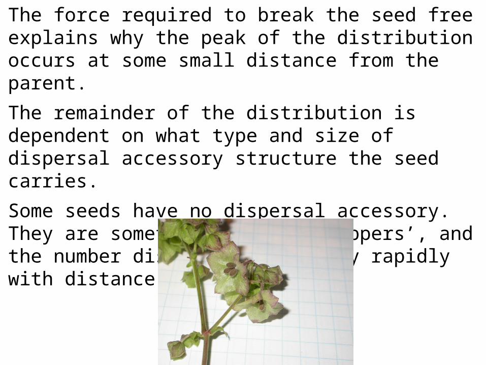
Some seeds have no dispersal accessory. They are sometimes called ‘ploppers’, and the number dispersed drops very rapidly with distance.

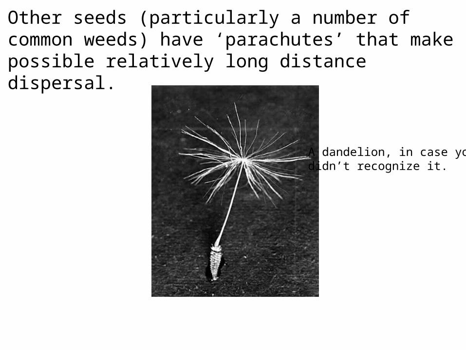
Other seeds (particularly a number of common weeds) have ‘parachutes’ that make possible relatively long distance dispersal.

A dandelion, in case youdidn’t recognize it.

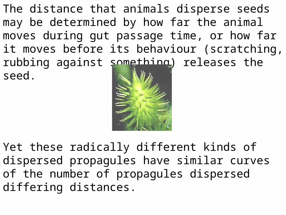
The distance that animals disperse seeds may be determined by how far the animal moves during gut passage time, or how far it moves before its behaviour (scratching, rubbing against something) releases the seed.

Yet these radically different kinds of dispersed propagules have similar curves of the number of propagules dispersed differing distances.

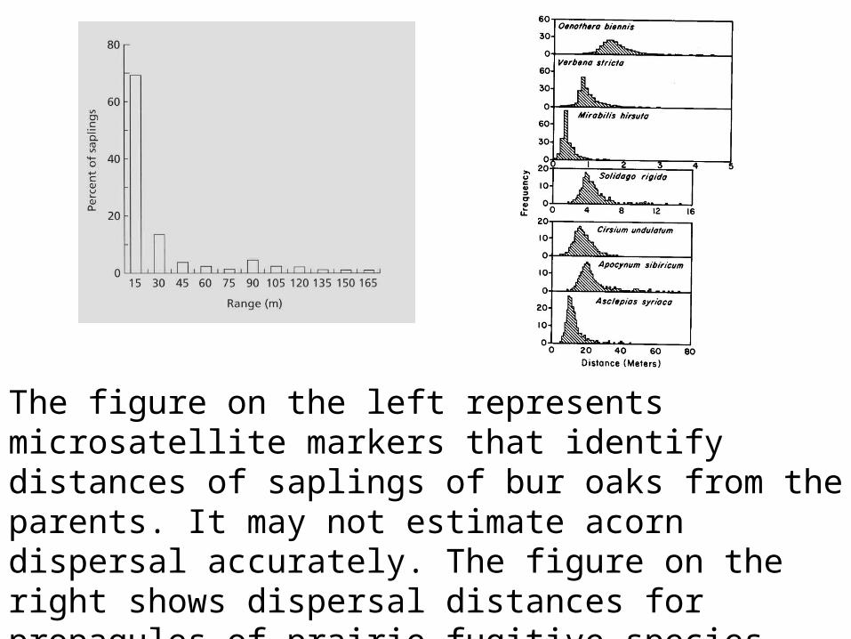
The figure on the left represents microsatellite markers that identify distances of saplings of bur oaks from the parents. It may not estimate acorn dispersal accurately. The figure on the right shows dispersal distances for propagules of prairie fugitive species. Note that here peaks are not at 0 distance.

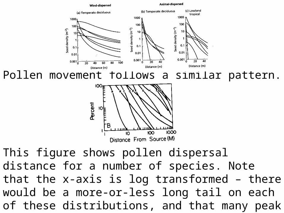
Pollen movement follows a similar pattern.

This figure shows pollen dispersal distance for a number of species. Note that the x-axis is log transformed – there would be a more-or-less long tail on each of these distributions, and that many peak meters from the parent. However, also note that pollen can travel much further, on average, than seeds.

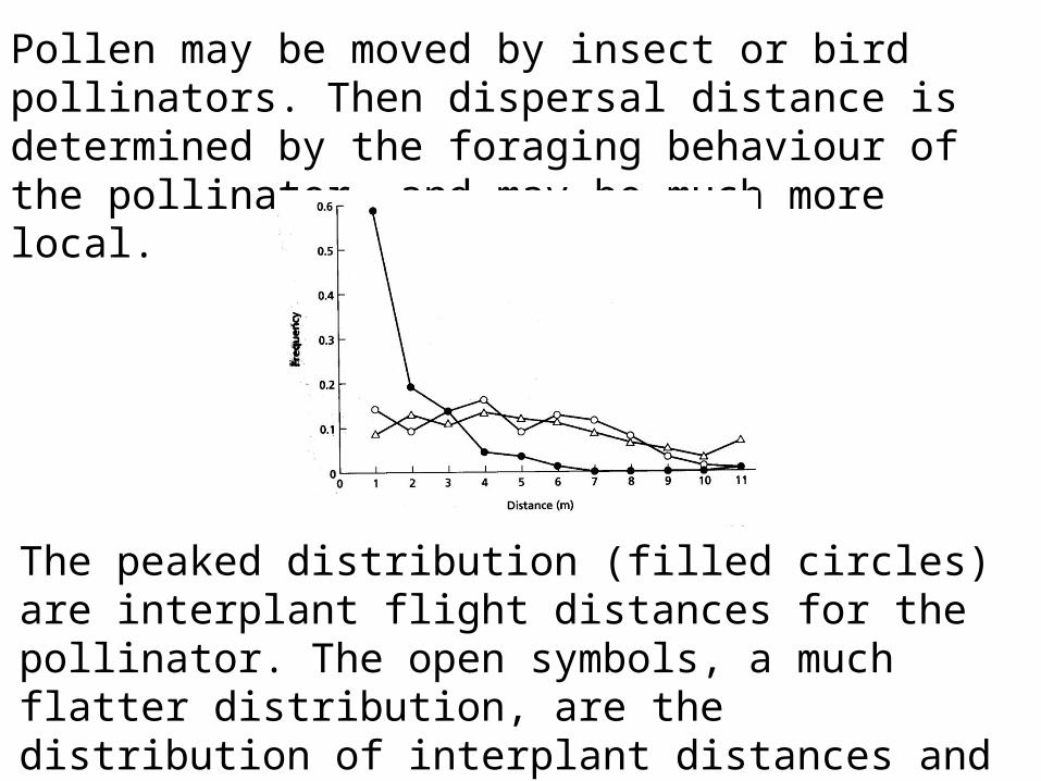
Pollen may be moved by insect or bird pollinators. Then dispersal distance is determined by the foraging behaviour of the pollinator, and may be much more local.

The peaked distribution (filled circles) are interplant flight distances for the pollinator. The open symbols, a much flatter distribution, are the distribution of interplant distances and that for realized pollen dispersal. The plant, Asclepias exultata, uses pollinia (packages of pollen grains).

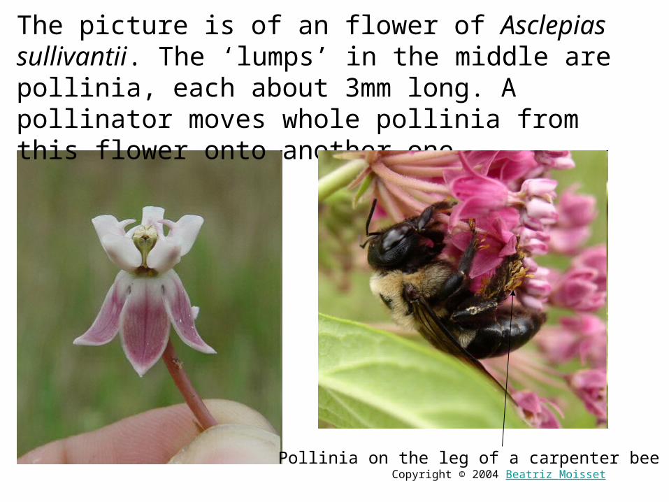
The picture is of an flower of Asclepias sullivantii. The ‘lumps’ in the middle are pollinia, each about 3mm long. A pollinator moves whole pollinia from this flower onto another one.

Pollinia on the leg of a carpenter bee Copyright © 2004 Beatriz Moisset

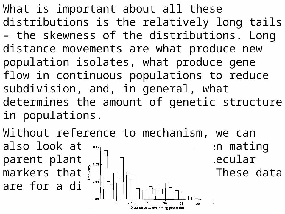
What is important about all these distributions is the relatively long tails – the skewness of the distributions. Long distance movements are what produce new population isolates, what produce gene flow in continuous populations to reduce subdivision, and, in general, what determines the amount of genetic structure in populations.

Without reference to mechanism, we can also look at the distance between mating parent plants (determined by molecular markers that reveal parentage). These data are for a dioecious lily.

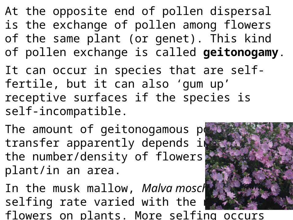
At the opposite end of pollen dispersal is the exchange of pollen among flowers of the same plant (or genet). This kind of pollen exchange is called geitonogamy.

It can occur in species that are self-fertile, but it can also ‘gum up’ receptive surfaces if the species is self-incompatible.

The amount of geitonogamous pollen transfer apparently depends in part on the number/density of flowers on a plant/in an area.

In the musk mallow, Malva moschata, selfing rate varied with the number of flowers on plants. More selfing occurs on plants with larger numbers of flowers (since bees probably spend longer moving among flowers on those plants).

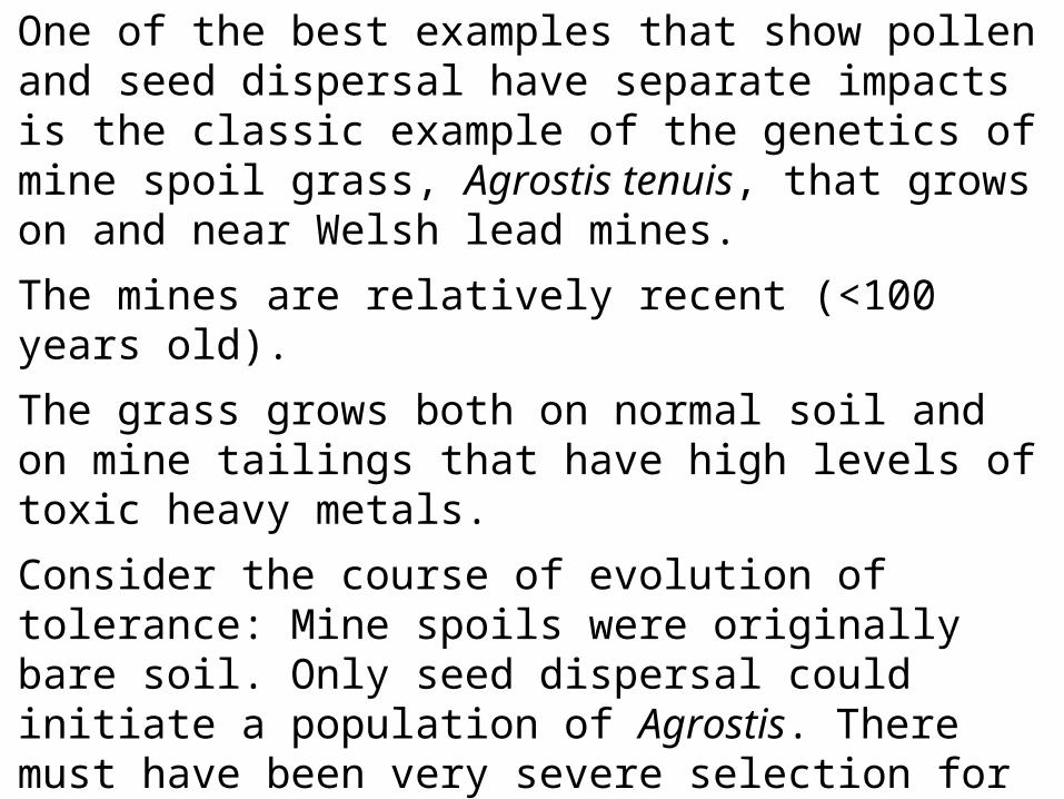
One of the best examples that show pollen and seed dispersal have separate impacts is the classic example of the genetics of mine spoil grass, Agrostis tenuis, that grows on and near Welsh lead mines.

The mines are relatively recent (<100 years old).

The grass grows both on normal soil and on mine tailings that have high levels of toxic heavy metals.

Consider the course of evolution of tolerance: Mine spoils were originally bare soil. Only seed dispersal could initiate a population of Agrostis. There must have been very severe selection for tolerance on seedlings and plants growing from those seeds.

Tolerant plants produce pollen carrying the tolerance gene(s).

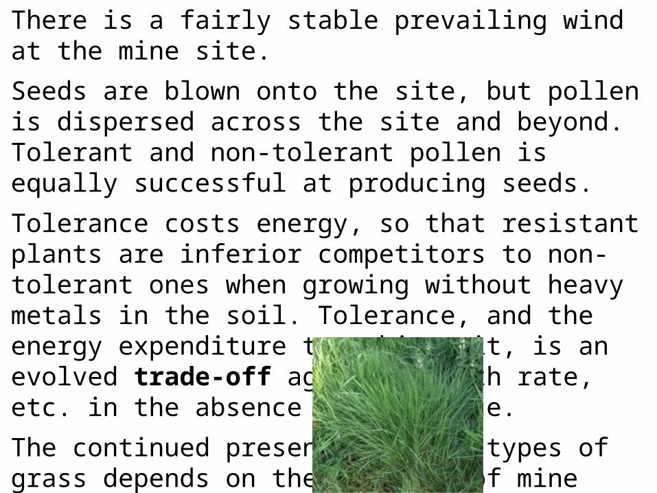
There is a fairly stable prevailing wind at the mine site.

Seeds are blown onto the site, but pollen is dispersed across the site and beyond. Tolerant and non-tolerant pollen is equally successful at producing seeds.

Tolerance costs energy, so that resistant plants are inferior competitors to non-tolerant ones when growing without heavy metals in the soil. Tolerance, and the energy expenditure to achieve it, is an evolved trade-off against growth rate, etc. in the absence of tolerance.

The continued presence of both types of grass depends on the presence of mine spoil soils.

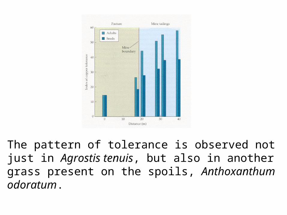
The pattern of tolerance is observed not just in Agrostis tenuis, but also in another grass present on the spoils, Anthoxanthum odoratum.

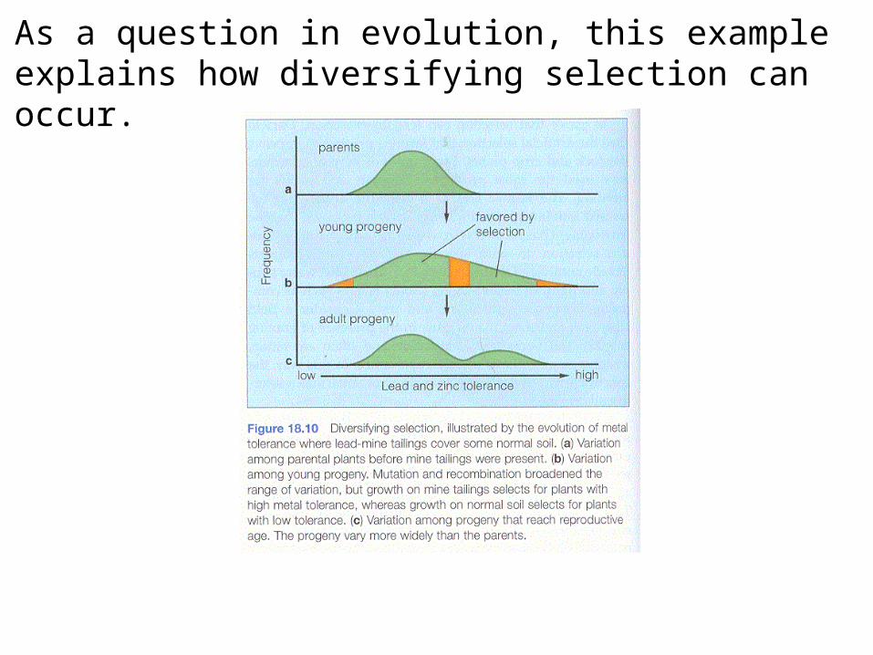
As a question in evolution, this example explains how diversifying selection can occur.

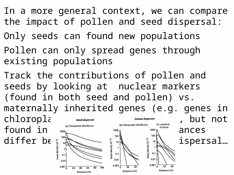
In a more general context, we can compare the impact of pollen and seed dispersal:

Only seeds can found new populations

Pollen can only spread genes through existing populations

Track the contributions of pollen and seeds by looking at nuclear markers (found in both seed and pollen) vs. maternally inherited genes (e.g. genes in chloroplasts and/or mitochondria, but not found in pollen). Dispersal distances differ between wind and animal dispersal…

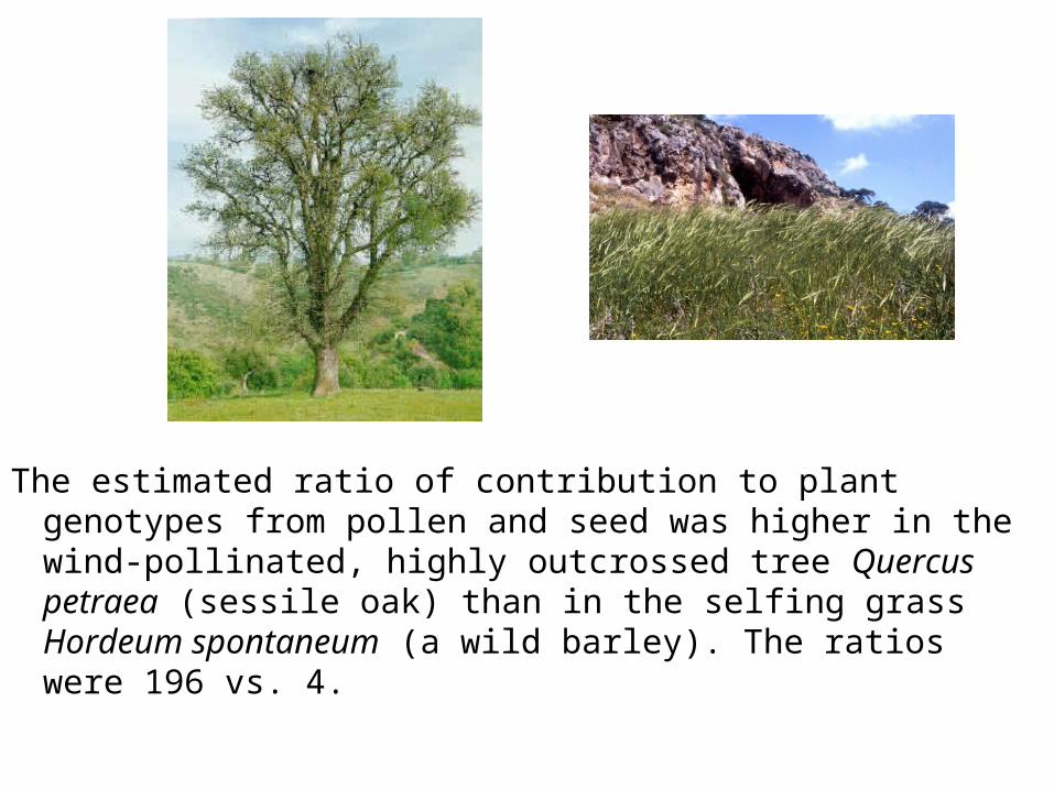
The estimated ratio of contribution to plant genotypes from pollen and seed was higher in the wind-pollinated, highly outcrossed tree Quercus petraea (sessile oak) than in the selfing grass Hordeum spontaneum (a wild barley). The ratios were 196 vs. 4.

Now we can consider one explanation of how selfing can be selectively advantageous:

Outcrossing plants growing at low density may fail to receive enough pollen to breed.

That can lead to selection for self-fertilization to assure reproduction. Fitness could be very low for a plant that can only outcross when it is isolated or its density is low.

This is one explanation for the breakdown in outcrossing systems at the edges of habitats and at the edges of species’ ranges.

This brings us back to considering isolation by distance…

The probability of two specific individuals mating decreases as the distance between them increases.

Combined with limited dispersal of seeds and pollen, neighbours tend to be related (their alleles originate from a common ancestor)

This leads to a genetic structure within a population– which we can look at as the likelihood that two randomly selected alleles have come from the same ancestor.

Some standard for that likelihood is used to measure neighborhood size - the size of an unstructured population that would produce the same probability of identity by descent.

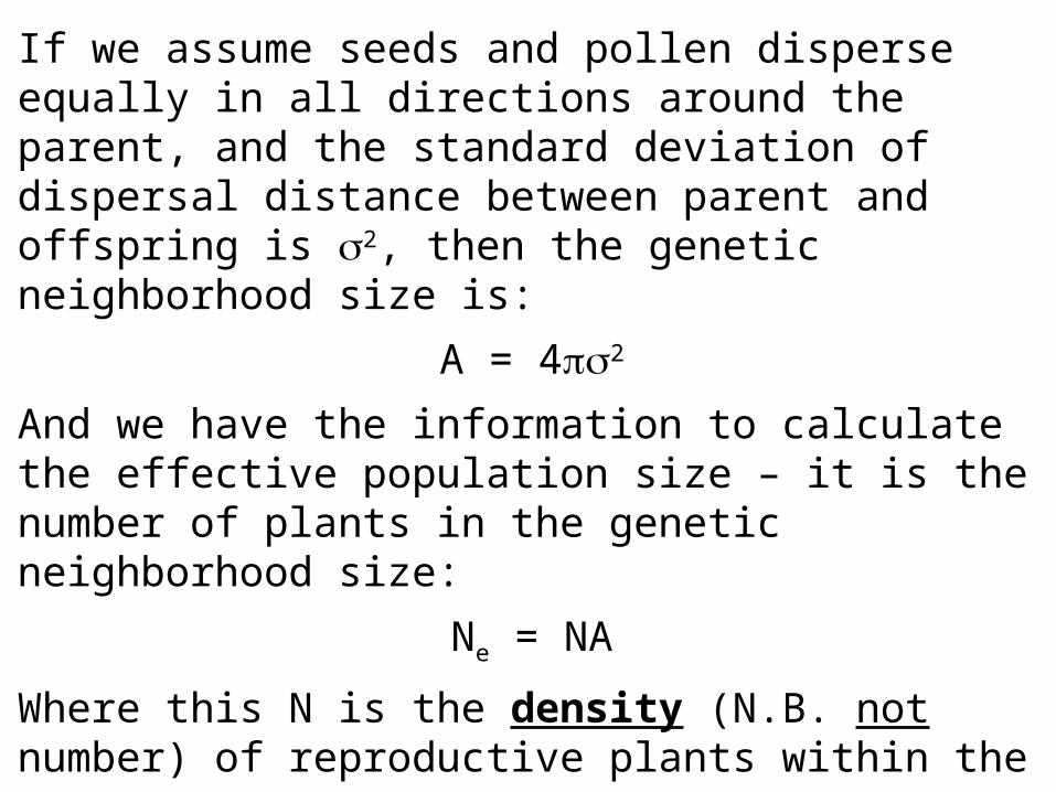
If we assume seeds and pollen disperse equally in all directions around the parent, and the standard deviation of dispersal distance between parent and offspring is 2, then the genetic neighborhood size is:

A = 42

And we have the information to calculate the effective population size – it is the number of plants in the genetic neighborhood size:

Ne = NA

Where this N is the density (N.B. not number) of reproductive plants within the area.

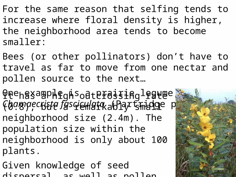
For the same reason that selfing tends to increase where floral density is higher, the neighborhood area tends to become smaller:

Bees (or other pollinators) don’t have to travel as far to move from one nectar and pollen source to the next…

One example is a prairie legume, Chamaecrista fasciculata (Partridge pea).

It has a high outcrossing rate (0.8), but a remarkably small neighborhood size (2.4m). The population size within the neighborhood is only about 100 plants.

Given knowledge of seed dispersal, as well as pollen movement, it was possible to partition the contributions:

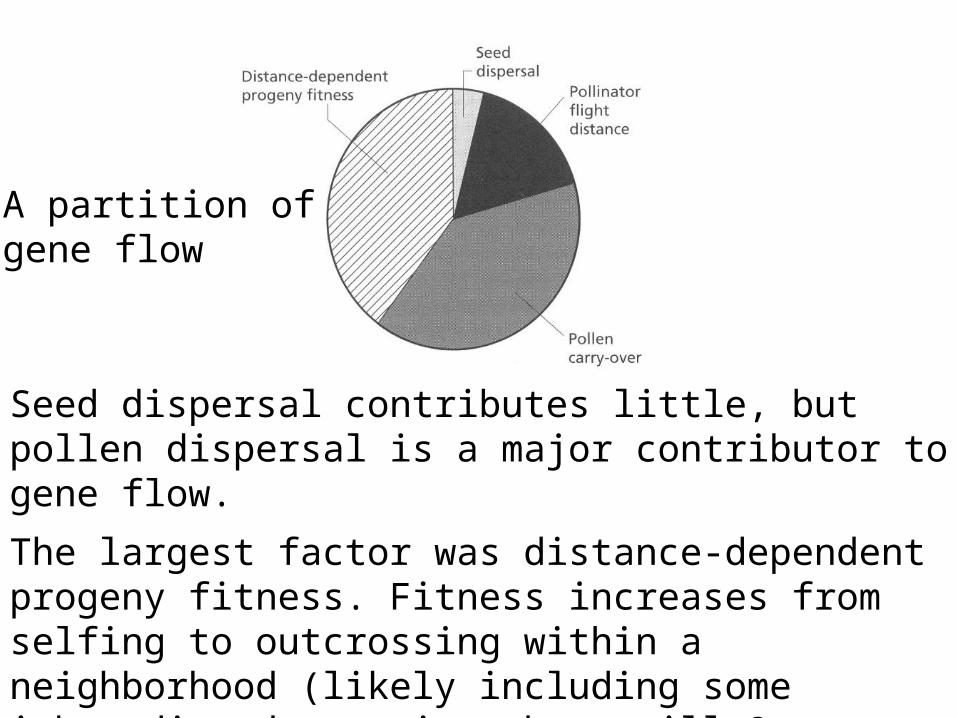
Seed dispersal contributes little, but pollen dispersal is a major contributor to gene flow.

The largest factor was distance-dependent progeny fitness. Fitness increases from selfing to outcrossing within a neighborhood (likely including some inbreeding depression, but still 2x selfing) to outcrossing involving parents more than one neighborhood radius apart.

A partition ofgene flow

The Founder Effect

Founders of a new population likely carry only a small sample of alleles present in the source.

Thus each new population will have differing allele frequencies.

Bottlenecks have a similar effect: reduction of a population to a small size that then recovers from surviving founders.

Both founder and bottleneck effects reduce genetic diversity.

The small sample of the founder population may not be representative of the allele frequencies present in the larger source population, and rare alleles may be missed.

At the population or species level, the loss of genetic diversity due to the founder effect should be small. Why?

Answer: Alleles lost in any group as a founder effect are likely to have been rare in the source population.

Those rare alleles contribute little to He (gene diversity, calculated from the frequencies of alleles at a locus as He = 1 - pi

2) they make negligible contribution – with small pi, their pi

2 will be small.

Alleles with intermediate or high frequency are likely to persist in newly founded populations.

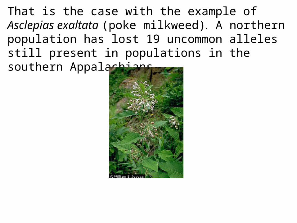
That is the case with the example of Asclepias exaltata (poke milkweed). A northern population has lost 19 uncommon alleles still present in populations in the southern Appalachians.

This leads to a broader principle: the Wahlund effect

Given lower genetic diversity in small subpopulations, due to founder effects, bottlenecks, or selection adapting the subpopulation to its local environment, there frequently are higher allele frequencies for the most common allele. What will the Hardy-Weinberg equilibrium frequencies look like in each subpopulation?

Assume p = 0.8 and q = 0.2

p2 = 0.64 - frequency of the common allele homozygote

2pq = 0.32 – frequency of heterozygotes

q2 = 0.04 – frequency or ‘rare’ homozygotes

Overall frequency of homozygotes is 0.68

If, in another subpopulation, these p and q are reversed, there will still be a higher fraction of homozygotes.

Averaged over the whole population, we would expect the usual 50% homozygotes, since total population p = q = 0.5.

However, given the effects of sampling (the founder effect, bottlenecks) and/or local selection, when we count homozygotes across the population we find an excess.

This excess is what is called the Wahlund effect.

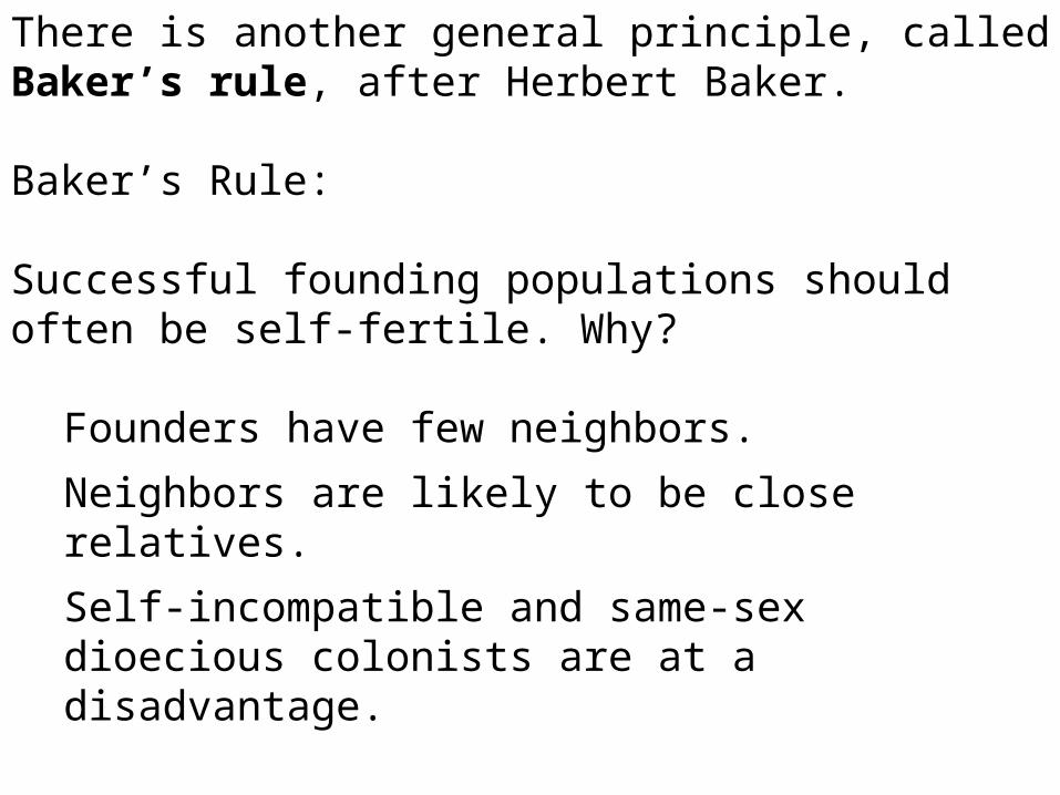
There is another general principle, called Baker’s rule, after Herbert Baker.

Baker’s Rule:

Successful founding populations should often be self-fertile. Why?

Founders have few neighbors.

Neighbors are likely to be close relatives.

Self-incompatible and same-sex dioecious colonists are at a disadvantage.

What are the patterns of genetic diversity in plant populations?

The patterns we see in genetic diversity are functions of effective population size and deme isolation.

Genetic drift causes a loss of genetic variation in isolated subpopulations and differentiation among them.

Inbreeding will accelerate subpopulation differentiation, since migration rates of alleles among subpopulations will be very low. Inbreeding also reduces effective population size and increases homozygosity.

Thus there should be lower genetic variation in inbred demes

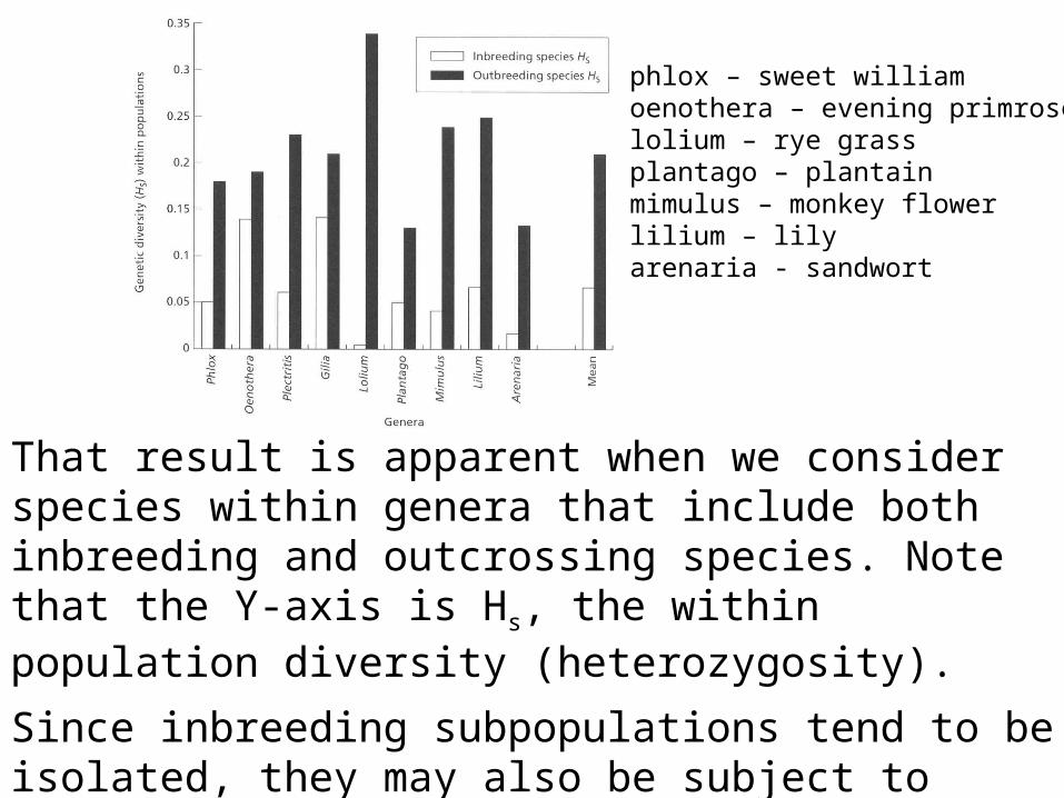
That result is apparent when we consider species within genera that include both inbreeding and outcrossing species. Note that the Y-axis is Hs, the within population diversity (heterozygosity).

Since inbreeding subpopulations tend to be isolated, they may also be subject to strong adaptive selection to local conditions, and that can also increase differences.

phlox – sweet williamoenothera – evening primroselolium – rye grassplantago – plantainmimulus – monkey flowerlilium – lilyarenaria - sandwort

In inbreeding populations, selection can choose the best adapted homozygote (or at least more likely to be a homozygote in these populations).

Inbreeding perpetuates that homozygote into subsequent generations.

If outcrossed, the successful phenotype may not be perpetuated; instead, a variety of phenotypes will be produced, only a fraction of which will be successful.

The table below shows mean proportion of genetic variation at allozyme loci for different breeding systems:

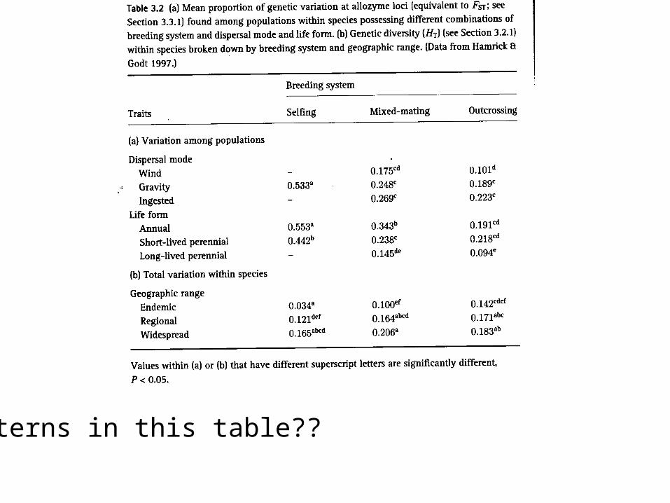
Patterns in this table??

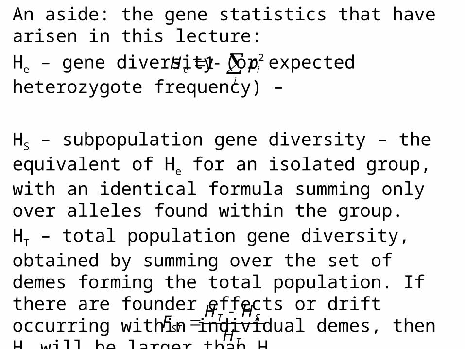
An aside: the gene statistics that have arisen in this lecture:

He – gene diversity (or expected heterozygote frequency) –

HS – subpopulation gene diversity – the equivalent of He for an isolated group, with an identical formula summing only over alleles found within the group.

HT – total population gene diversity, obtained by summing over the set of demes forming the total population. If there are founder effects or drift occurring within individual demes, then HT will be larger than HS.

FST – the between population proportion of gene diversity (or, in different words, the extent to which individuals in subpopulations are more similar than in the total set of populations) -

i

ie pH 21

T

STST H

HHF